Stability of a Stochastic Ring Network

Abstract

In this paper we establish a necessary and sufficient stability condition for a stochastic ring network. Such networks naturally appear in a variety of applications within communication, computer, and road traffic systems. They typically involve multiple customer types and some form of priority structure to decide which customer receives service. These two system features tend to complicate the issue of identifying a stability condition, but we demonstrate how the ring topology can be leveraged to solve the problem.

Keywords. Cellular automata $\diamond$ Communication networks $\diamond$ Fluid models $\diamond$ Ring-topology queueing networks $\diamond$ Stability and bottleneck analysis $\diamond$ Traffic flow theory

Affiliations.

Pieter Jacob Storm^†: Department of Mathematics and Computer Science, Eindhoven University of Technology, Eindhoven, The Netherlands.

Wouter Kager: Department of Mathematics, Vrije Universiteit Amsterdam, Amsterdam, The Netherlands.

Michel Mandjes^†: Korteweg–de Vries Institute for Mathematics, University of Amsterdam, Amsterdam, The Netherlands; Eurandom, Eindhoven University of Technology, Eindhoven, The Netherlands; Amsterdam Business School, Faculty of Economics and Business, University of Amsterdam, Amsterdam, The Netherlands.

Sem Borst^†: Department of Mathematics and Computer Science, Eindhoven University of Technology, Eindhoven, The Netherlands.

^†Partly funded by NWO Gravitation project Networks, grant number 024.002.003.

1 Introduction

This paper deals with the analysis of a hybrid cellular automaton and queueing network model with a ring structure. Specifically, customers (particles) are routed probabilistically between stations (cells) according to a network with a ring topology, and customers within the ring have priority over exogenously arriving customers. Application domains of such networks include packet-switched optical ring networks [19, 35, 36], road traffic intersections in the form of roundabouts [2, 31], multiprocessor systems with ring-based nanophotonic on-chip networks [5, 18], and medium access control (MAC) protocols for Local Area Networks (LANs) [33, 12].

The model that we consider was proposed as a discrete-time Markov chain in [31]. The main contribution of this paper is a necessary and sufficient condition for stability (i.e., positive recurrence) of the model. This proves the conjecture on the stability region in [31]. Our main result also implies that the stability condition is sufficient for the slotted-ring model studied in [33] to be stable in a particular sense (see Section 6.1 for details). In [33], this result was only shown to hold under the rather strong additional assumption that, among other things, sequences of certain characteristic inter-event times of the system are asymptotically strongly stationary, and the ergodic rates at which these events occur are well-defined. Our paper proves that this assumption is unnecessary, and is in fact implied by the stability condition.

Stability (or positive recurrence) of a Markov process is a fundamental condition for many theorems in Markov chain theory that are commonly used to study stationary or asymptotic properties. The mathematical theory of stability is well-developed [10, 25, 26]. However, for queueing models that involve multiple customer classes and priorities, like the one in this paper, determining conditions for stability remains a notoriously difficult task. In particular, many instances with such features exist where a subcritical system load (i.e., an arrival rate strictly below 1 of each station’s normalized workload) is not sufficient for stability [6, 22, 24, 28, 29]. Moreover, the model that we consider does not have a product-form stationary distribution [31], which makes it impossible to determine a stability condition from the normalization of the stationary measure. As it turns out, though, we can leverage the specific routing topology of a ring model to formally establish the stability condition.

An important consequence of the necessity and sufficiency of the stability condition is that this condition can be interpreted as the system capacity. Specifically, it implies that the set of arrival rates for which the model is stable is monotone, meaning that the system does not lose its property of positive recurrence when arrival rates are decreased. This monotonicity is not automatic for multiclass networks with priorities, see [15] for an example. In the context of communication systems and road traffic, capacity is an important measure for the load that the system is able to process; see, e.g., [9, 23] for similar recent work in this area.

We prove the stability condition for the model in [31] using a fluid model approach. More precisely, we establish a coupling between the Markov chain associated with the model and the queue length process of a multiclass queueing network, such that they follow the same sample paths up to a bijection. As a consequence, proving positive recurrence of the Markov chain can be reduced to proving stability of the simpler fluid model associated with the multiclass network [13, 8]. We prove the stability of the fluid model with an approach based on [32], with some modifications that are required in our context. This approach exploits the relationship between the stability condition and the marginal stationary rate at which segments of the ring are occupied when the model is stable.

As mentioned earlier, stochastic ring networks that involve queues are ubiquitous within communication and transportation systems. In these domains, priority service for traffic on the ring over exogenously arriving traffic is natural to create free flow on the ring, so as to avoid collisions and eliminate the need for buffering within the ring. Additionally, the destination of a packet (or vehicle) typically depends on where it entered the ring, giving rise to multiple customer types. The combination of these properties (a ring, a priority structure, and multiple customer types) motivates the specific model we consider in this paper.

In the context of communication networks, ring topologies are the cornerstone of various widely deployed architectures, and our model pertains to LANs with slotted-ring MAC protocols [12, 33, 34, 37] as well as Wavelength-Division Multiplexing (WDM) based Metropolitan Area Networks (MANs) with packet switching or optical burst switching, see [4, Section 4.1] and [17, 19, 35, 36]. Nowadays, ring-topology waveguides are a standard component in optical networks because of their ability to transmit large amounts of data via light in a short amount of time [11, 20, 30]. While current networks mostly rely on wavelength routing, optical burst switching and packet switching mechanisms offer finer granularity and more dynamic resource sharing, and thus allow for higher efficiency and bandwidth utilization, especially with bursty and unpredictable traffic patterns.

Ring structures are also encountered in traffic networks as a form of intersection design, known as a roundabout. On a roundabout, vehicles traverse an intersection via a circulating ring to which several roads are attached that function as on- and off-ramps. Vehicles on the circulating ring have priority over vehicles in the attached legs, cf. [2, 31]. These properties make them very similar, both in function and dynamics, to rings in communication systems, as described above. The results in this paper apply to a model that was originally proposed for single-lane roundabouts [31].

The outline of the paper is as follows. We start by introducing the model in Section 2. Section 3 provides a preliminary analysis, introduces the stability condition, and states our main theorem. In Section 4 we couple the model to a multiclass queueing network. We then proceed by proving stability of this multiclass queueing network in Section 5 using fluid limits. Finally, Section 6 discusses related models to which our results can be applied directly and possible extensions to other models, and Section 7 concludes.

Notation. Unless otherwise specified, all random variables and processes are defined on a common probability space $(\,\Omega,\mathcal{F},\mathbb{P}\,)$. We write $\mathbb{Z}_{+}$ for the non-negative integers, $\mathbb{N}$ for the natural numbers (i.e., $\mathbb{N}\equiv\mathbb{Z}_{+}\setminus\{0\}$), $\mathbb{R}$ for the real numbers, and $\mathbb{R}_{+}$ for the set of non-negative reals. For any dimension $d$, $\lvert\,\cdot\,\rvert$ denotes the $L^{1}$-norm on elements of $\mathbb{R}^{d}$. If $a$ and $b$ are real numbers, then $a\wedge b$ is the minimum and $a\vee b$ the maximum of $a$ and $b$.

2 Model description

As we mentioned in the introduction, the model we consider is a stochastic ring network that has a variety of application domains, but was originally introduced as a model for a roundabout in [31]. In this section, to describe the model, we stay close to the original formulation as a roundabout model and use the related (road traffic) terminology. For technical reasons, which we will explain in Section 6, we consider a version of the model that differs slightly from the roundabout model in [31]. For the model we consider, we identify and prove a necessary and sufficient condition for stability. This result also identifies the global stability regions for the model in [31] and the slotted-ring model in [33], as we formally show in Section 6.

The roundabout model is a slotted ring consisting of $L$ cells, with on-ramp queues in front of each cell. The cells and queues are indexed by $i\in\{1,\ldots,L\}$, with cell 1 adjacent to cell $L$; using this cyclic structure, we allow ourselves to use the index $i+\nobreak L$ to refer to cell/queue $i$. The presence of vehicles on the roundabout is modeled by the state of the cells. Each cell can either be empty, or contain a vehicle that has entered the roundabout at some cell $j$. In the first case we say the state of cell $i$ is 0 and in the second case we say that its state is $j$; we will also say that a cell is occupied by a vehicle of type $j$ when the state of the cell is $j$. The queues model vehicles waiting to enter the roundabout, and their state is a number in $\mathbb{Z}_{+}$.

The model has discrete-time dynamics. The main idea is that vehicles arrive via the queues to the roundabout, traverse a number of cells to an off-ramp, and depart the roundabout. At each time $t\in\nobreak\mathbb{Z}_{+}$, if there are vehicles in queue $i$ and cell $i$ is empty, one vehicle from the queue will enter the roundabout and occupy cell $i+\nobreak 1$ at time $t+\nobreak 1$. If cell $i$ is occupied by a vehicle of type $j$, then the vehicle will either depart from the system with probability $q_{ij}\in[0,1]$, or occupy cell $i+\nobreak 1$ at the next time step. We emphasize that the probability $q_{ij}$ depends on $j$ to reflect that the cell at which a vehicle leaves the system may depend on where it entered. To model arriving vehicles, we impose that at every time step, a new vehicle will arrive to queue $i$ with probability $p_{i}\in[0,1]$. We assume that all decisions whether a vehicle arrives at a cell $i$ and whether a vehicle of type $j$ will leave cell $i$ (if present), are made independently of each other and of the current state and history of the process (see Appendix A for an explicit construction of the process). Note that on-ramps and off-ramps can be removed by setting arrival or departure probabilities equal to zero.

We now provide a more precise account of these dynamics by formulating update rules for the system (as is customary for cellular automata). These rules are local in the sense that we only need to know the current joint states of queue $i$ and cell $i$, and can disregard the remainder of the system, to determine the new states of queue $i$ and cell $i+\nobreak 1$ (in accordance with the cellular automata paradigm). It turns out that we need to distinguish three cases:

• cell $i$ and queue $i$ are both empty. In this case, no vehicle can enter the roundabout from queue $i$ and cell $i+\nobreak 1$ will be empty the next time step. If a new vehicle arrives to queue $i$ (which happens with probability $p_{i}$), then queue $i$ will have length 1 at the next time step. Otherwise, it will have length zero.

• cell $i$ is empty and queue $i$ is not empty. Then, the vehicle at the front of queue $i$ will enter the roundabout and move on to cell $i+\nobreak 1$ in the process. Thus, cell $i+\nobreak 1$ will be in state $i$ one unit of time later. Queue $i$ either remains at its current length (if a new vehicle arrives to queue $i$), or its length decreases by one.

• cell $i$ is occupied by a type-$j$ vehicle. In this case, queue $i$ is blocked, hence its length will grow by one if a new vehicle arrives, or will stay the same otherwise. The vehicle in cell $i$ will either leave the system with probability $q_{ij}$, in which case cell $i+\nobreak 1$ will be empty one unit of time later, or the vehicle remains in the system, so that cell $i+\nobreak 1$ will be in state $j$ at the next time step.

Having specified the precise dynamics of the model, we observe that if for type-$j$ vehicles, $q_{ij}=0$ for each $i\in\{1,\ldots,L\}$, then such vehicles cannot leave the network. We therefore require that $\prod_{\ell=1}^{L}(1-q_{\ell j})<1$ for each $j\in\{1,\ldots,L\}$, so that any vehicle eventually leaves the network. Additionally, note that when $p_{i}=1$ for some $i\in\{1,\ldots,L\}$, then queue $i$ can never decrease in length. Since our focus is on stability, we impose $p_{i}\in[0,1)$ for all $i\in\{1,\ldots,L\}$.

3 Stability condition and main result

The model under consideration is a discrete-time Markov chain, which we denote by $X^{1}(\cdot)=\{X^{1}(t)\colon t\in\mathbb{Z}_{+}\}$. The associated state space is $\mathcal{S}^{1}:=(\mathbb{Z}_{+}\times\{0,\ldots,L\})^{L}$, the set of vectors in $\mathbb{R}^{2L}$ that describe the state of each cell and queue. We observe that $X^{1}(\cdot)$ is irreducible on the set of states that can be reached from the empty state, since from any state, with strictly positive probability, we can empty the system in a finite number of steps. Note that specific choices of the $p_{i}$ and $q_{ij}$ can make it impossible to reach all states in the state space. In addition, $X^{1}(\cdot)$ is aperiodic as we can remain in the empty state for an arbitrary (finite) number of time steps, with strictly positive probability.

Following [8, 13, 25], we say that $X^{1}(\cdot)$ is stable when it is positive recurrent. In Section 3.1, we will derive an explicit expression for the marginal stationary distribution of the states of the cells under the assumption of stability. This result was already obtained in [31], but here we use a different method based on the system’s offered load. To be more precise, we show that when the system is stable, the marginal stationary probability that cell $i$ is in state $j$ is equal to $p_{j}$ times the expected number of times that a vehicle of type $j$ will occupy cell $i$ during the time it spends on the roundabout. This connection leads us to formulate a necessary and sufficient condition for stability in Section 3.2, which is our main result. Moreover, this connection plays an important role in our proof that the condition is sufficient in Section 5. We prove the necessity of the condition for stability at the end of Section 3.2.

3.1 Marginal stationary distribution

In our formulation of the model given above, we update the system at each time step by checking for external arrivals, and deciding for each vehicle on the roundabout whether or not it leaves. As a consequence of the dynamics, the time spent on the roundabout by each vehicle that enters the roundabout at cell $j$ is an independent copy of a generic random variable $T_{j}$, the distribution of which is completely determined by the parameters $q_{ij}$. We use this fact in this subsection to derive the marginal stationary distribution of the states of the cells when the system is stable, and again in Section 5 to prove our main result.

To be precise, $T_{j}$ is a random variable with distribution given by

$$\begin{cases}\mathbb{P}(T_{j}=0)=0;\\[5.0pt] \mathbb{P}(T_{j}=k)=\prod_{\ell=j+1}^{j+k-1}(1-q_{\ell j})\,q_{j+k,j}&\text{for $k\geq 1$},\end{cases}$$ (1)

where we adopt the convention that the empty product is equal to 1, and define $q_{\ell j}$ for $\ell>L$ by setting $q_{\ell j}:=q_{ij}$ whenever $\ell\equiv i\pmod{L}$. Observe that the model dynamics determine the distribution of the $T_{j}$ and that different distributions could be considered as well. Such model extensions do not significantly impact our analysis and are discussed in Section 6.3.

Observe that the number of times a vehicle of type $j$ that spends time $T_{j}$ on the roundabout will occupy cell $i$ before leaving, is also a well-defined random variable. We denote it by $N_{ij}$, and we set $b_{ij}:=\mathbb{E}N_{ij}$. In our model, $b_{ij}$ is the expected number of visits to cell $i$ by a vehicle that moves onto the roundabout from the on-ramp at cell $j$. We next define, for $i\in\{1,2,\dots,L\}$,

$$\pi_{ij}:=\begin{cases}b_{ij}\,p_{j}&\text{if $j\in\{1,2,\dots,L\}$};\\ 1-\sum_{j=1}^{L}b_{ij}\,p_{j}&\text{if $j=0$}.\end{cases}$$ (2)

The numbers $\pi_{ij}$ have an important interpretation in case the model is stable:

Proposition (Marginal stationary distribution).

If the model is stable, then the marginal stationary probability that cell $i$ is in state $j$ is the number $\pi_{ij}$ defined by (2).

Proof.

Suppose that the model is stable. Then the long-term rate at which type-$j$ vehicles move onto the roundabout must be equal to the rate at which such vehicles arrive, which is $p_{j}$ by the strong law of large numbers. Again by the strong law of large numbers, it follows that the long-term fraction of time cell $i$ is occupied by a type-$j$ vehicle is $p_{j}\,b_{ij}$. By the ergodic theorem, this number is also the marginal stationary probability that cell $i$ is in state $j$. ∎

As we show below, for our model the numbers $b_{ij}$ can be expressed explicitly in terms of the parameters $q_{ij}$ by the following formula:

$$b_{ij}=\begin{cases}\displaystyle\frac{\prod_{\ell=j+1}^{i+L-1}(1-q_{\ell j})}{1-\prod_{\ell=1}^{L}(1-q_{\ell j})}&\quad\text{if $1\leq i\leq j\leq L$};\\[18.0pt] \displaystyle\frac{\prod_{\ell=j+1}^{i-1}(1-q_{\ell j})}{1-\prod_{\ell=1}^{L}(1-q_{\ell j})}&\quad\text{if $1\leq j<i\leq L$}.\end{cases}$$ (3)

For example, if $L=1$ we have $b_{11}=q_{11}^{-1}$ because the time a vehicle spends on the roundabout follows a geometric distribution with parameter $q_{11}$. For $L=2$, formula (3) gives

$$b_{12}=\frac{1}{1-(1-q_{12})(1-q_{22})}\quad\text{and}\quad b_{22}=\frac{1-q_{12}}{1-(1-q_{12})(1-q_{22})}$$

for vehicles of type 2. This is explained as follows. Note that a vehicle of type 2 first enters cell 1 when it moves onto the roundabout. The vehicle’s return probability to cell 1 is $(1-q_{12})(1-q_{22})$, hence the above expression for $b_{12}$ is indeed the expected number of visits to cell 1. The expected number of visits to cell 2 is then $(1-q_{12})\,b_{12}$ because $1-q_{12}$ is the probability the vehicle moves on to cell 2 when it occupies cell 1. We now prove (3) in the general case:

Lemma .

For all $i,j\in\{1,\dots,L\}$ we have that $b_{ij}=\mathbb{E}N_{ij}$ is given by (3) if $T_{j}$ has the distribution specified by (1).

Proof.

Consider the case $1\leq j<i\leq L$. Note that the probability distribution of $N_{ij}$ can be expressed in terms of the distribution of $T_{j}$ as

$$\mathbb{P}(N_{ij}\geq n+1)=\mathbb{P}(T_{j}\geq i-j+nL),\qquad n\geq 0.$$

From (1) it follows by induction in $k$ that

$$\mathbb{P}(T_{j}\geq k)=\prod_{\ell=j+1}^{j+k-1}(1-q_{\ell j}),\qquad k\geq 1.$$

Combining these observations, we obtain

$$\mathbb{P}(N_{ij}\geq n+1)=\prod_{\ell=j+1}^{i-1}(1-q_{\ell j})\biggl{(}\,\prod_{\ell=1}^{L}(1-q_{\ell j})\biggr{)}^{n},$$

and summing both sides over all $n\geq 0$ yields formula (3) for $b_{ij}=\mathbb{E}N_{ij}$. The proof in the case $1\leq i\leq j\leq L$ is similar. ∎

Remark .

We saw in the proof of Proposition 3.1 that $\pi_{ij}$ represents the long-term fraction of time cell $i$ is occupied by a type-$j$ vehicle when the model is stable. But the quantity $\pi_{ij}$ is also meaningful if the system is unstable, since it is by definition only a measure of the load imposed on the system. The question of stability deals with whether or not all the vehicles manage to get onto the roundabout. If the system is unstable, the $\pi_{ij}$ still describe the load that is offered to the system, but we cannot use ergodicity to conclude that $\pi_{ij}$ is the fraction of time cell $i$ will be occupied by a vehicle of type $j$. Our characterization of the $\pi_{ij}$ in terms of $\mathbb{E}N_{ij}$ plays an important role in proving the main theorem (Theorem 3.1 below).

3.2 Condition for stability

Under the assumption that the system is stable, the Markov chain $X^{1}(\cdot)$ has a stationary distribution $\pi$. In the previous section we have shown that the vector $\{\pi_{i0},\pi_{i1},\dots,\pi_{iL}\}$ given by (2) and (3) is then the marginal stationary distribution of cell $i$, for $i=1,2,\dots,L$. In particular, $\pi_{i0}$ is the stationary rate at which cell $i$ is empty when the system is stable. Since vehicles arrive at cell $i$ at rate $p_{i}$ and can only enter onto the roundabout when the cell is empty, it seems reasonable to believe that the system cannot be stable if $p_{i}>\pi_{i0}$ for some cell $i$. Conversely, one would suspect that if $p_{i}<\pi_{i0}$ for all cells $i$, the cells will be vacant often enough to prevent the queues from blowing up. It turns out that the latter condition is in fact not only sufficient, but also necessary for the system to be stable:

Theorem 3.1 (Main result).

A necessary and sufficient condition for the roundabout model to be stable (by which we mean that the Markov chain $X^{1}(\cdot)$ is positive recurrent) is that

$$p_{i}<\pi_{i0}=1-\sum_{j=1}^{L}b_{ij}\,p_{j}\qquad\text{for all~{}$i\in\{1,2,\dots,L\}$}.$$

For example, in the case $L=1$, the expected time a vehicle occupies the cell is $b_{11}=q_{11}^{-1}$, as we saw in Section 3.1. It follows that the expected time that elapses after a vehicle enters the roundabout until the next vehicle can enter is $1+q_{11}^{-1}$, because the cell has to be empty for at least one unit of time before it can be occupied again. Hence, for the system to be stable, the arrival rate $p_{1}$ must be smaller than $1/\bigl{(}1+q_{11}^{-1}\bigr{)}$, which is precisely what the stability condition of Theorem 3.1 says. Now consider the case $L=2$. Suppose we fix the arrival rate $p_{2}$. Then vehicles of type 2 already lay a claim on cell 1 for a fraction $b_{12}\,p_{2}$ of the time. During the remaining fraction of time, like in the case $L=1$, the maximum rate at which cell 1 can be empty if we also allow type-1 vehicles onto the roundabout is $(1+b_{11})^{-1}$. This leads to the stability condition $p_{1}<(1-b_{12}\,p_{2})(1+b_{11})^{-1}$, and an analogous condition for $p_{2}$ can be derived by reversing the roles of the type-1 and type-2 vehicles. The stability region consists of the pairs $(p_{1},p_{2})$ that satisfy both inequalities (see Figure 1). In general, for any $L$, the stability condition is a system of linear inequalities for the arrival rates $p_{i}$, and hence the stability region is a convex polytope contained in $[0,1)^{L}$ with the zero vector as one of its corners.

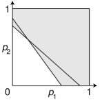
Figure 1: The stability region (unshaded area) for $L=2$, $q_{11}=q_{12}=0.75$, $q_{21}=q_{22}=0.5$.

The hard part of the theorem is to prove that the stated condition is indeed sufficient for the stability of the system. We close this section with a proof of the necessity of the stability condition; Sections 4 and 5 are devoted to proving the sufficiency. One may also wonder about transience in case the stability condition does not hold; this is discussed in Section 7.

Proposition .

The condition that $p_{i}<\pi_{i0}$ for all $i\in\{1,2,\dots,L\}$ is a necessary condition for the stability of the roundabout model.

Proof.

We know that the Markov chain $X^{1}(\cdot)$ is aperiodic and irreducible. Assume furthermore that the system is stable, that is, that $X^{1}(\cdot)$ is also positive recurrent. Then $X^{1}(\cdot)$ has a stationary distribution $\pi$, and since the Markov chain is irreducible, the state in which every cell and every queue is empty must have a strictly positive probability, which we denote by $\pi_{\varnothing}$, under the stationary distribution.

Suppose that we start our Markov chain from the stationary distribution $\pi$. Let $C_{i}(t)$ denote the state of cell $i$ at time $t$, and let $Q_{i}(t)$ be the length of queue $i$ at time $t$. Write $A_{i}(t)$ for the event that a new vehicle arrives at cell $i$ at time $t$. Then the queue length process satisfies

$$\begin{split}Q_{i}(t+1)&=Q_{i}(t)+\mathds{1}_{\{Q_{i}(t)>0\}}\bigl{(}\mathds{1}_{A_{i}(t+1)}-\mathds{1}_{\{C_{i}(t)=0\}}\bigr{)}+\mathds{1}_{\{Q_{i}(t)=0\}}\mathds{1}_{A_{i}(t+1)}\\ &=Q_{i}(t)+\mathds{1}_{A_{i}(t+1)}-\mathds{1}_{\{C_{i}(t)=0\}}+\mathds{1}_{\{Q_{i}(t)=C_{i}(t)=0\}},\end{split}$$

from which it follows that

$$\frac{1}{n}Q_{i}(n)=\frac{1}{n}Q_{i}(0)+\frac{1}{n}\sum_{t=0}^{n-1}\mathds{1}_{A_{i}(t+1)}-\frac{1}{n}\sum_{t=0}^{n-1}\mathds{1}_{\{C_{i}(t)=0\}}+\frac{1}{n}\sum_{t=0}^{n-1}\mathds{1}_{\{Q_{i}(t)=C_{i}(t)=0\}}.$$ (4)

We now want to take $n\to\infty$ in (4). On the one hand, since we assumed the model is stable, it is clear that we must have that

$$\liminf_{n\to\infty}\frac{1}{n}Q_{i}(n)=0\qquad\text{a.s.}$$

On the other hand, the first term on the right hand side in (4) clearly converges almost surely to 0 as $n\to\infty$, whereas the second term converges a.s. to $p_{i}$ by the strong law of large numbers, and the third term converges a.s. to $-\pi_{i0}$ by the ergodic theorem. As for the last term in (4), we observe that the event that the system is completely empty is a subset of the event $\{Q_{i}(t)=C_{i}(t)=0\}$, so that by the ergodic theorem we can conclude that

$$\liminf_{n\to\infty}\frac{1}{n}\sum_{t=0}^{n-1}\mathds{1}_{\{Q_{i}(t)=C_{i}(t)=0\}}\geq\pi_{\varnothing}>0.$$

Combining these observations, it follows that almost surely,

$$0=\liminf_{n\to\infty}\frac{1}{n}Q_{i}(n)\geq 0+p_{i}-\pi_{i0}+\pi_{\varnothing}>p_{i}-\pi_{i0}.$$

Hence, $p_{i}$ must be strictly smaller than $\pi_{i0}$ for every cell $i$ if the roundabout model is stable. ∎

4 Multiclass queueing network formulation

To prove sufficiency of the stability condition in Theorem 3.1, we formulate in this section a multiclass network (explained below) that has essentially the same dynamics as the roundabout model from Section 2. That is, for each choice of parameters $p_{i}$ and $q_{ij}$, $i,j\in\{1,\dots,L\}$, for the roundabout model we define an analogous multiclass network, using the same parameters to define the appropriate exogenous arrival and routing processes in the network. We shall refer to a choice of these parameters as a parameter setting. The two model formulations can be coupled on a sample-path level, formalized in Lemma 4 below. This allows us in Section 5 to utilize the powerful fluid model framework for multiclass queueing networks to prove stability of the multiclass-network formulation of our model, hence proving it for the model in the original formulation as well.

A multiclass queueing network, or simply multiclass network, is a network consisting of a finite collection of (single server) stations serving customers from a finite number of customer classes. Each customer class has its own queue at one of the stations, with its own exogenous arrival process and service time distribution. After service completion, customers are either routed to another queue (and associated customer class), or depart from the network. In addition, a multiclass network can have other characteristics relating to specific model applications, such as customer class priorities in stations and blocking features.

Fix a parameter setting. To map the roundabout model to a multiclass network, we identify each cell $i$ with a station $i$ in the multiclass network. Vehicles that arrive from outside to the on-ramp of cell $i$ become customers of class $(i,0)$ in the multiclass network, and vehicles of type $j$ that occupy cell $i$ become class $(i,j)$ customers. Thus, there are $L$ stations and $L(L+\nobreak 1)=L^{2}+\nobreak L$ customer classes in the multiclass network. The set of customer classes is

$$\mathcal{K}:=\bigl{\{}(i,j)\colon i\in\{1,\ldots,L\},j\in\{0,\ldots,L\}\bigr{\}},$$

and station $i$ serves the customers of all classes $(i,j)$ with $j\in\{0,\dots,L\}$. We will now define the exogenous arrival processes, service time distributions, routing policy, and priority structure that will make the multiclass network mimic the dynamics of the roundabout model. As an aid to the reader, Figure 2 illustrates the multiclass network and its routing policy.

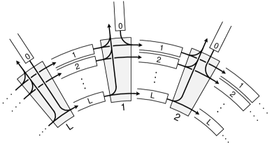
Figure 2: The multiclass queueing network. The shaded boxes are the stations and the queues are labeled with the corresponding vehicle type (using $0$ for external arrivals). The arrows show how customers can be routed through the network from the $L+1$ queues at each station.

First, to account for the external arrivals, the exogenous arrival process for class $(i,0)$ customers clearly must have independent, geometrically distributed inter-arrival times with parameter $p_{i}$. All other customer classes $(i,j)$ with $i,j\in\{1,\dots,L\}$ have no exogenous arrivals; such customers can appear in the network only because they arrive as a class $(j,0)$ customer and are subsequently routed in the network to become a class $(i,j)$ customer. This corresponds in the roundabout model to a vehicle entering onto the roundabout at cell $j$, and then traversing a number of cells to reach cell $i$.

To mimic this behavior correctly in the multiclass network, we impose that the service times are exactly one unit of time for each class of customer. Furthermore, after completing service at station $i$, a class $(i,0)$ customer is routed to the next station and becomes a customer of class $((i\bmod L)+\nobreak 1,i)$. Likewise, a class $(i,j)$ customer is either routed to the next station with probability $1-\nobreak q_{ij}$, or leaves the network. This routing policy is captured by the routing matrix $P$. The rows and columns of this matrix are indexed by the set of customer classes $\mathcal{K}$, and the entry $P_{ij,k\ell}$ defines the probability that a class $(i,j)$ customer is routed to become a class $(k,\ell)$ customer after service completion, and is therefore given by

$$P_{ij,k\ell}=\begin{cases}1&\text{if $j=0$, $k=(i\bmod L)+1$, $\ell=i$;}\\ 1-q_{ij}&\text{if $j\neq 0$, $k=(i\bmod L)+1$, $\ell=j$;}\\ 0&\text{otherwise.}\end{cases}$$ (5)

Next, we need to account for the fact that in the roundabout model, any vehicle that occupies a cell blocks the corresponding on-ramp and is guaranteed to move out of that cell after one unit of time. We therefore impose the following priority structure on the multiclass network: for each $i\in\{1,\dots,L\}$, customers of classes $(i,j)$ with $j\in\{1,\dots,L\}$ have priority over class $(i,0)$ customers. This means that class $(i,0)$ customers only receive service at station $i$ if the queues associated with class $(i,j)$ customers with $j\neq 0$ are all empty.

Finally, we need to consider the restriction in the roundabout model that each cell can be occupied by at most one vehicle at a time. For the multiclass network this means that we have to guarantee that, for each station $i$, the combined number of customers of classes $(i,j)$ with $j\neq 0$ is at most 1 at all times. But we can achieve this by simply imposing this condition on the initial state of the network: if at time 0, for each station $i$, the combined number of customers of classes $(i,j)$ with $j\in\{1,\dots,L\}$ is at most 1, then the same is automatically true for all times $t\in\nobreak\mathbb{Z}_{+}$, because all service times are exactly 1, class $(i,j)$ customers with $j\neq 0$ have priority over class $(i,0)$ customers, and customers can only be routed to one of the queues at station $i$ by the previous station in the network. Henceforth, we only consider the multiclass network under this condition on the initial state.

It is well known (see, e.g., [13, Section 2] or [8, Section 4.1]) that a multiclass network can be represented as a Markov chain. In our case, due to the geometric inter-arrival times, deterministic service times and discrete-time nature of the network, we can represent it as a discrete-time Markov chain with a discrete state space. We denote this Markov chain by $X^{2}(\cdot)$, and take as our state space $\mathcal{S}^{2}:=(\mathbb{Z}_{+}\times\mathcal{V})^{L}$, where $\mathcal{V}:=\{x\in\{0,1\}^{L}\colon\sum_{k}x_{k}\leq 1\}$. Thus, each state is a vector in $\mathbb{R}^{\scriptscriptstyle L^{2}+L}$ that tells us, for every customer class, how many of those customers are present in the network. Because of the way we constructed the multiclass network, there is a natural bijection between the two state spaces $\mathcal{S}^{1}$ and $\mathcal{S}^{2}$, and it is possible to couple the two Markov chains $X^{1}(\cdot)$ and $X^{2}(\cdot)$ in such a way that they follow the same sample paths up to this bijection. We formalize this claim in the following lemma, the proof of which is given for completeness in Appendix A:

Lemma .

For any fixed parameter setting, there exists a coupling of $X^{1}(\cdot)$ and $X^{2}(\cdot)$ and a bijection $f\colon\mathcal{S}^{1}\to\mathcal{S}^{2}$ such that for every $\omega\in\Omega$, if $f\bigl{(}X^{1}(\omega,0)\bigr{)}=X^{2}(\omega,0)$, then

$$f\bigl{(}X^{1}(\omega,t)\bigr{)}=X^{2}(\omega,t)\qquad\text{for all~{}$t\in\mathbb{Z}_{+}$.}$$

Lemma 4 allows us to complete the proof of Theorem 3.1 by proving that the stability condition implies stability of $X^{2}(\cdot)$. For this we can rely on the theory of fluid limits and Foster–Lyapunov functions, cf. [8, 9, 13, 23].

5 Proof of the main result

This section of the paper is dedicated to proving that $X^{2}(\cdot)$ is stable if the stability condition in Theorem 3.1 is satisfied. By Lemma 4 and Proposition 3.2, this completes the proof of Theorem 3.1. Nowadays there is a standardized approach for proving stability of multiclass queueing networks, which utilizes the powerful framework of fluid limits and stability of the associated fluid model. For a complete exposition of this technique we refer to [8], which is based on work that goes back to [28, 13, 7]. We begin our proof in Section 5.1 by writing down the set of queueing equations that describe the dynamics of the multiclass network in terms of simple stochastic processes, for which we derive the associated fluid model in Section 5.2. We then complete the proof of stability in Section 5.3 by making use of the fluid model.

5.1 The queueing equations

For $i$ in $\{1,\ldots,L\}$, let $A_{i0}(\cdot):=\{A_{i0}(t)\colon t\in\mathbb{Z}_{+}\}$ be the stochastic process that counts the cumulative number of exogenous class $(i,0)$ arrivals up to time $t$. For $i,j$ in $\{1,\ldots,L\}$ we set $A_{ij}(\cdot)\equiv 0$, reflecting that the customer class $(i,j)$ has no exogenous arrivals. Let $Q^{x}_{ij}(t)$ denote the length of the queue containing class $(i,j)$ customers at time $t\in\mathbb{Z}_{+}$, where $x$ denotes the initial state of the system. This defines the queue length processes $Q^{x}_{ij}(\cdot):=\{Q^{x}_{ij}(t)\colon t\in\mathbb{Z}_{+}\}$. Note that they can be combined into a vector-valued process that has the same law as the Markov chain $X^{2}(\cdot)$ starting from the state $x$. We set $T^{x}_{ij}(\cdot):=\{T^{x}_{ij}(t)\colon t\in\mathbb{Z}_{+}\}$, where $T^{x}_{ij}(t)$ is the cumulative amount of service time that has been spent by station $i$ on class $(i,j)$ customers up to time $t$. As the service times of each customer class are precisely one unit of time, $T^{x}_{ij}(t)$ is also equal to the total number of class $(i,j)$ service completions up to time $t$.

Recall that $\mathcal{K}$ is the set of customer classes. For each class $(i,j)$ we introduce the random vector $\phi^{ij}(n)$ with components $\phi^{ij}_{k\ell}(n)$, $(k,\ell)\in\mathcal{K}$, where $\phi^{ij}_{k\ell}(n)=1$ if the $n$th class $(i,j)$ customer served by station $i$ is routed to the class $(k,\ell)$ queue, and $\phi^{ij}_{k\ell}(n)=0$ otherwise. Observe that $\phi^{ij}(n)$ is an $(L^{2}+\nobreak L)$-dimensional random vector with expectation $(P_{ij})^{\top}$, where $P_{ij}$ is the row of the routing matrix $P$ corresponding to the index $(i,j)$. For each class $(i,j)$ we thus have an i.i.d. sequence of routing vectors $\{\phi^{ij}(n)\colon n\in\mathbb{N}\}$. Define the cumulative routing process as $\Phi^{ij}(\cdot):=\{\Phi^{ij}(n)\colon n\in\mathbb{Z}_{+}\}$, where $\Phi^{ij}(0):=0$ and $\Phi^{ij}(n):=\sum_{k=1}^{n}\phi^{ij}(k)$ for $n\geq 1$. With this definition, $\Phi^{ij}_{k\ell}(n)$ counts the number of class $(i,j)$ customers that have been routed to the queue of class $(k,\ell)$ customers after the first $n$ service completions of class $(i,j)$ customers.

For each class $(i,j)$, the stochastic processes $A_{ij}(\cdot)$ and $\Phi^{k\ell}_{ij}(\cdot)$, $T^{x}_{k\ell}(\cdot)$ for all $(k,\ell)\in\mathcal{K}$ completely determine the paths of the queue length process $Q^{x}_{ij}(\cdot)$. To be precise, for each time $t$ we can calculate $Q^{x}_{ij}(t)$ by adding the exogenous arrivals and the arrivals via routing to the initial queue length, and subtracting the departures. Thus we have for all $t\in\mathbb{Z}_{+}$

$$Q_{ij}^{x}(t)=Q_{ij}^{x}(0)+A_{ij}(t)+\sum\nolimits_{(k,\ell)\in\mathcal{K}}\Phi^{k\ell}_{ij}\bigl{(}T_{k\ell}^{x}(t)\bigr{)}-T_{ij}^{x}(t),\vphantom{\sum}$$ (6)

$$\text{$Q_{ij}^{x}(t)\geq 0$ and $Q^{x}_{ij}(t+1)-Q^{x}_{ij}(t)\in\{-1,0,1\}$},\vphantom{\sum\nolimits_{(k,\ell)}}$$ (7)

$$T_{ij}^{x}(t) t T_{ij}^{x}(t+1)-T_{ij}^{x}(t)\leq 1 T_{ij}^{x}(0)=0$$ is non-decreasing in , , and . (8)

The multiclass network has the work-conserving property, which means that a station will not idle whenever at least one of its queues is non-empty. To express this property in a formula, for $i\in\{1,\ldots,L\}$ and $t\in\mathbb{Z}_{+}$, let $I^{x}_{i}(t)$ denote the cumulative amount of time that station $i$ has been idle up to time $t$, and write $\Delta I^{x}_{i}(t):=I^{x}_{i}(t+1)-I^{x}_{i}(t)$. Then

$$I_{i}^{x}(t):=t-\sum_{j=0}^{L}T_{ij}^{x}(t) t$$ is non-decreasing in , (9)

$$\text{$\sum_{t=0}^{\infty}\sum_{j=0}^{L}Q_{ij}^{x}(t)\,\Delta I_{i}^{x}(t)=0$ for all $i\in\{1,\ldots,L\}$}.\vphantom{\sum}$$ (10)

Similarly to the way in which (10) captures the work-conserving property, we can also account for the priorities in the system. Recall that we imposed that customers of classes $(i,j)$ with $j\neq 0$ have priority over class $(i,0)$ customers. If we let $I^{x}_{i0}(t):=t-\sum_{j=1}^{L}T^{x}_{ij}(t)$ be the total service time available for class $(i,0)$ customers up to time $t$ at station $i$, and write $\Delta I^{x}_{i0}(t):=I^{x}_{i0}(t+1)-I^{x}_{i0}(t)$, then the priority structure is captured by the priority equation

$$\text{$\sum_{t=0}^{\infty}\sum_{j=1}^{L}Q^{x}_{ij}(t)\,\Delta I^{x}_{i0}(t)=0$ for all $i\in\{1,\ldots,L\}$}.\vphantom{\sum}$$ (11)

For each sample path of the multiclass network, the associated processes $Q^{x}_{ij}(\cdot)$ and $T^{x}_{ij}(\cdot)$ have to satisfy equations (6)–(11). We refer to this set of equations as the queueing equations or the queue length process representation. The evolution of the sample paths clearly depends on the parameter setting, i.e., these equations are parameterized by the collection of $p_{i}$ and $q_{ij}$.

5.2 The fluid model

We are now ready to introduce the fluid model equations, or fluid model for short. They are continuous-time analogs of the queueing equations that arise naturally by taking a scaling limit of solutions to the queueing equations. To introduce these fluid model equations, it is convenient to first extend all the discrete-time processes introduced in Section 5.1 to continuous time by linear interpolation. That is, we define $Q_{ij}^{x}(t)$ for non-integer values of $t\in\mathbb{R}_{+}$ by interpolating linearly between $Q^{x}_{ij}\bigl{(}\lfloor t\rfloor\bigr{)}$ and $Q^{x}_{ij}\bigl{(}\lfloor t\rfloor+1\bigr{)}$, and we extend the other processes introduced in Section 5.1 to continuous time in the same way. Furthermore, we switch to a vector notation by defining $Q^{x}(\cdot):=\{Q^{x}(t)\colon t\in\mathbb{R}_{+}\}$ as the vector-valued process with components $Q^{x}_{ij}(\cdot)$, $(i,j)\in\mathcal{K}$. Likewise, we define $T^{x}(\cdot)$ as the process with components $T^{x}_{ij}(\cdot)$. All vectors are column vectors, and (in)equalities between vectors have to be read component-wise.

To obtain the fluid model, we scale the queue length and service time processes by the norm of the initial state $x$. That is, we introduce the scaled processes $SQ^{x}(\cdot)$ and $ST^{x}(\cdot)$ by setting

$$SQ^{x}(t):=\frac{\;\>1}{\lvert x\rvert\vee 1}\,Q^{x}\bigl{(}\lvert x\rvert t\bigr{)}\quad\text{and}\quad ST^{x}(t):=\frac{\;\>1}{\lvert x\rvert\vee 1}\,T^{x}\bigl{(}\lvert x\rvert t\bigr{)}$$

for each $t\in\mathbb{R}_{+}$. We claim that for any sequence of initial states with norm tending to $\infty$, these scaled processes converge at almost every sample point along a subsequence to limit processes $\bar{Q}(\cdot)$ and $\bar{T}(\cdot)$ which we refer to as a fluid limit. Moreover, this fluid limit has to satisfy fluid model analogs of the queueing equations (6)–(11). The first three of those equations are

$$\bar{Q}(t)=\bar{Q}(0)+p\,t-(I-P^{\top})\,\bar{T}(t),\vphantom{\sum}$$ (12)

$$\text{$\bar{Q}(t)\geq 0$ and each component of~{}$\bar{Q}(\cdot)$ is Lipschitz-1},\vphantom{\sum}$$ (13)

$$\text{$\bar{T}(t)$ is non-decreasing in~{}$t$, each component of~{}$\bar{T}(\cdot)$ is Lipschitz-1, and $\bar{T}(0)=0$},\vphantom{\sum}$$ (14)

where $I$ denotes the identity matrix of dimension $L^{2}+L$ and $p$ is the vector with components $p_{ij}$ for $(i,j)\in\mathcal{K}$ defined by $p_{i0}:=p_{i}$ and $p_{ij}:=0$ if $j\neq 0$. Next we have the two equations

$$\text{$\bar{I}(t):=e\,t-C\,\bar{T}(t)$ is non-decreasing in~{}$t$},\vphantom{\sum}$$ (15)

$$\text{$\int_{0}^{\infty}\bar{Q}_{i0}(t)\mathop{}\!\mathrm{d}\bar{I}_{i}(t)=0$ for all $i\in\{1,\ldots,L\}$},\vphantom{\sum}$$ (16)

where $e$ is the $L$-dimensional vector of ones and $C$ is the incidence matrix linking each station to the customer classes served by that station; it has dimension $L\times(L^{2}+L)$ and entries defined for $i\in\{1,\dots,L\}$ and $(j,k)\in\mathcal{K}$ by $C_{i,jk}=1$ if $j=i$ and $C_{i,jk}=0$ otherwise. Finally,

$$\text{$\bar{Q}_{ij}(\cdot)\equiv 0$ for all $i,j\in\{1,\ldots,L\}$}.\vphantom{\sum}$$ (17)

It may not be obvious that this last equation captures the priority structure in the fluid limit, but note that (17) together with (12) yields $\bar{T}_{ij}(t)=\sum_{(k,\ell)\in\mathcal{K}}\bar{T}_{k\ell}(t)\,P_{k\ell,ij}$ for $i,j\in\{1,\dots,L\}$. This says that in the fluid limit, the stations must instantly spend service time on customers who enter the ring to route them through the network, reflecting their priority.

We refer to equations (12)–(17) as the fluid model equations or fluid model. Every pair of functions $\bar{Q}(\cdot),\bar{T}(\cdot)$ that is a solution to these equations is called a fluid model solution. Our claims about convergence to a fluid limit which is a fluid model solution are made precise in the following theorem. A general version of this result has been proven in [13] for continuous-time multiclass networks. Because of the discrete-time nature of our processes, the proof of the theorem requires some small modifications, and is therefore given in Appendix B.

Theorem 5.1.

There exists a set of sample points $\Omega^{\prime}\subset\Omega$ with $\mathbb{P}(\Omega^{\prime})=1$ such that for every sequence of initial states $\{x^{\prime}_{n}\}$ with $\lvert x^{\prime}_{n}\rvert\to\infty$, we can find for each $\omega\in\Omega^{\prime}$ a subsequence $\{x^{\prime\prime}_{n}(\omega)\}$ and functions $\bar{Q}(\omega,\cdot),\bar{T}(\omega,\cdot)$ so that everywhere on $\Omega^{\prime}$ (omitting $\omega$ from the notation),

$$\sup_{t\in[0,m]}\,\bigl{\lvert}SQ^{x^{\prime\prime}_{n}}(t)-\bar{Q}(t)\bigr{\rvert}\vee\bigl{\lvert}ST^{x^{\prime\prime}_{n}}(t)-\bar{T}(t)\bigr{\rvert}\to 0\qquad\text{as $n\to\infty$}$$ (18)

for all $m\in\mathbb{N}$. Moreover, on $\Omega^{\prime}$, the pair $\bar{Q}(\cdot),\bar{T}(\cdot)$ is a fluid model solution with $\lvert\bar{Q}(0)\rvert=1$.

5.3 Stability of the fluid model

In this section we complete the proof of Theorem 3.1, with an appeal to Lemma 4, by proving that the multiclass network defined in Section 4 is stable under the stability condition of the theorem. The key is to prove stability of the fluid model, which is defined as follows:

Definition .

We say that the fluid model (12)–(17) is stable if there exists a constant $\delta>0$ that depends only on $p$ and $P$ such that any fluid model solution $\bar{Q}(\cdot),\bar{T}(\cdot)$ with $\lvert\bar{Q}(0)\rvert=1$ satisfies $\bar{Q}(t)=0$ for all $t\geq\delta$.

It is well-known that in general, stability of the fluid model is a sufficient condition for stability of $X^{2}(\cdot)$. This result has been proven for Markov chains with general state spaces under an additional condition, e.g., see [13, Theorem 4.2] or [8, Theorem 4.16]. In the setting of a countable state space, a considerably shorter argument is given in [9]. For completeness, we formulate this key result in the following proposition, a proof of which is included in Appendix B.

Proposition .

If the fluid model is stable, then the Markov chain $X^{2}(\cdot)$ is positive recurrent.

So all that remains is to prove that, under the stability condition in Theorem 3.1, the fluid model is stable. A more general version of this result is proven in [16, Section 6], but here we present a more transparent proof based on [32]. It is shown in [32] that under deterministic assumptions on the external arrivals and routing in a ring network, any work-conserving policy stabilizes the ring. These assumptions are satisfied in our case because in the fluid limit, the arrival and routing processes become deterministic due to the strong law of large numbers (this is one of the key steps in the proof of Theorem 5.1 in Appendix B).

In our proof that the fluid model is stable, we consider the residual amount of time stations will be busy, given the amount of fluid mass that is present in the network. In essence, the goal of the proof is to show that this quantity, and hence the total fluid mass, must become zero before a fixed deterministic time that is determined only by the parameter setting. This means that we require a stronger result than the main theorem in [32], which (translated to our context) states only that the total fluid mass goes to zero in the limit $t\to\infty$. Moreover, traffic in [32] leaves the ring as soon as it reaches its destination, whereas fluid mass in our model can complete multiple full circles (albeit instantly) before being removed. This means that the quantities we consider, such as the residual work, are slightly different than the ones used in [32], and we also need to adapt the argument to obtain the stronger result we require.

It is customary in the theory of multiclass queueing networks to consider the quantities

$$\lambda:=\bigl{(}I-P^{\top}\bigr{)}^{-1}p\qquad\text{and}\qquad\rho:=C\lambda.$$

The quantity $\lambda$ is known as the solution of the traffic equations [8, Section 1.2], and $\lambda_{ij}$ can be interpreted as the effective arrival rate to the queue of class $(i,j)$ customers. By summing over $j$ we obtain the effective arrival rate at station $i$, given by $\rho_{i}=(C\lambda)_{i}=\sum_{j=0}^{L}\lambda_{ij}$. In any multiclass network, $\rho_{i}$ represents the amount of service time that arrives to the network per unit time and is required from station $i$ in the future. One can prove that the multiclass network cannot be stable when $\rho<1$ fails to hold, using an argument similar to the one we used to prove Proposition 3.2. In many cases $\rho<1$ is sufficient for stability, although this is not always true (see [8, Chapter 3] for counter-examples). The next lemma establishes that the condition for stability in Theorem 3.1 is equivalent to the condition that $\rho<1$.

Lemma .

For all $i\in\{1,\dots,L\}$ we have $\rho_{i}=p_{i}+1-\pi_{i0}$ and hence

$$\rho_{i}<1\quad\text{if and only if}\quad\pi_{i0}>p_{i}.$$

Proof.

Let $i\in\{1,\ldots,L\}$. We will show that $\rho_{i}=p_{i}+\sum_{j=1}^{L}b_{ij}\,p_{j}$, where we recall from Section 3.1 that $b_{ij}$ was defined in the roundabout model as the expected number of visits to cell $i$ by a type-$j$ vehicle that enters the roundabout. We start by observing that

$$\rho=C\bigl{(}I-P^{\top}\bigr{)}^{-1}p=C\biggl{(}I+\sum_{m=1}^{\infty}\bigl{(}P^{\top}\bigr{)}^{m}\biggr{)}\,p.$$

Hence, using the definition (5) of the routing matrix $P$ and the fact that $p_{i0}=p_{i}$ and $p_{ij}=0$ for $j\neq 0$, we obtain

$$\rho_{i}=\sum_{j=0}^{L}p_{ij}+\sum_{j=0}^{L}\sum_{m=1}^{\infty}\sum_{(k,\ell)\in\mathcal{K}}(P^{m})_{k\ell,ij}\,p_{k\ell}=p_{i}+\sum_{j=1}^{L}\sum_{m=1}^{\infty}(P^{m})_{j0,ij}\,p_{j}.$$

Here, $(P^{m})_{j0,ij}$ is the probability that a class $(j,0)$ customer is routed to become a class $(i,j)$ customer in $m$ steps, which is the same as the probability in the roundabout model that a vehicle that enters the roundabout at cell $j$ visits cell $i$ after having stayed on the roundabout for $m-\nobreak 1$ time steps. Hence, we see that $\rho_{i}$ is equal to $p_{i}+\sum_{j=1}^{L}b_{ij}\,p_{j}$, and we are done. ∎

The proof that the fluid model is stable hinges on another crucial lemma concerning the residual amount of work for each station $i$ at a given time. We claim that this quantity is described by the process $\bar{R}(\cdot):=\bigl{\{}\bar{R}(t)\colon t\in\mathbb{R}_{+}\bigr{\}}$ defined through

$$\bar{R}(t):=C\bigl{(}I-P^{\top}\bigr{)}^{-1}\bar{Q}(t).$$ (19)

To see that this process describes the residual work in the system, note first of all the analogy with the definition of $\rho$ as $C\bigl{(}I-P^{\top}\bigr{)}^{-1}p$. Since we have both $p_{ij}=0$ and, by (17), $\bar{Q}_{ij}(t)=0$ for $j\neq 0$, we can repeat the steps in the proof of Lemma 5.3 with $\bar{Q}(t)$ in place of $p$ to see that

$$\bar{R}_{i}(t)=\bar{Q}_{i0}(t)+\sum_{j=1}^{L}b_{ij}\,\bar{Q}_{j0}(t).$$ (20)

By definition, $b_{ij}$ is the mean number of times a customer who arrives at station $j$ in the multiclass network (i.e., a class $(j,0)$ customer) intends to visit station $i$ (as a class $(i,j)$ customer) in the future. It follows that we can indeed interpret $\bar{R}_{i}(t)$ as the residual amount of work for station $i$ that is present in the system at time $t$.

This quantity has an important property, which is the fluid equivalent of the statement that in the multiclass network, when the queue of class $(i,0)$ customers is empty, all customers who are present in the system and will visit station $i$, must also visit the preceding station $i-\nobreak 1$. This crucially reflects the ring topology in our system, and enables us to control the decay of the amount of fluid in the fluid model. We formulate this key result in the following lemma:

Lemma .

If $\bar{Q}(\cdot),\bar{T}(\cdot)$ is a fluid model solution, then for all $i\in\{1,\ldots,L\}$ and $t\geq 0$,

$$\bar{Q}_{i0}(t)=0\quad\text{implies}\quad\bar{R}_{i-1}(t)\geq\bar{R}_{i}(t),$$

where $i-1$ has to be read as $L$ when $i=1$.

Proof.

Let $t\geq 0$ be arbitrary and assume $\bar{Q}_{i0}(t)=0$. Let $k:=L-(L+\nobreak 1-\nobreak i\mod L)$ denote the station preceding station $i$ in the network. Then, using (20), we have

$$\begin{split}\bar{R}_{k}(t)-\bar{R}_{i}(t)&=\bar{Q}_{k0}(t)+\sum_{j=1}^{L}\sum_{m=1}^{\infty}(P^{m})_{j0,kj}\,\bar{Q}_{j0}(t)-\sum_{j=1}^{L}\sum_{m=1}^{\infty}(P^{m})_{j0,ij}\,\bar{Q}_{j0}(t)\\ &=\bar{Q}_{k0}(t)-\sum_{j=1}^{L}P_{j0,ij}\,\bar{Q}_{j0}(t)+\sum_{j=1}^{L}\sum_{m=1}^{\infty}\bigl{(}(P^{m})_{j0,kj}-(P^{m+1})_{j0,ij}\bigr{)}\,\bar{Q}_{j0}(t).\end{split}$$

Since $P_{k0,ik}=1$ and $P_{j0,ij}=0$ for $j\neq k$, the first two terms on the right cancel each other. Furthermore, since for $m\geq 1$, a class $(j,0)$ customer who is routed to become a class $(i,j)$ customer in $m+1$ steps must first be routed to become a class $(k,j)$ customer after $m$ steps, each term under the sum over $m$ is non-negative. Hence, $\bar{R}_{k}(t)\geq\bar{R}_{i}(t)$. ∎

We are now ready to state and prove the main result of this section, the stability of the fluid model under the condition $\rho<1$ from Lemma 5.3, which also completes the proof of Theorem 3.1.

Theorem 5.2.

If $\rho_{i}<1$ for each $i\in\{1,\dots,L\}$, then the fluid model (12)–(17) is stable.

Proof.

Assume $\max_{i}\rho_{i}<1$ and let the pair $\bar{Q}(\cdot),\bar{T}(\cdot)$ be a solution of the fluid model equations with $\lvert\bar{Q}(0)\rvert=1$. We first show that for this solution, the residual work for any station $i$ decreases at rate $1-\rho_{i}$ during time intervals in which the class $(i,0)$ queue is continuously non-empty. To see this, note that combining (19) and (12) gives $\bar{R}(t)=\bar{R}(0)+\rho\,t-C\,\bar{T}(t)$. So by (15), we can express $\bar{R}_{i}(t)$ in terms of the cumulative idle time process of station $i$ as

$$\bar{R}_{i}(t)=\bar{R}_{i}(0)-(1-\rho_{i})\,t+\bar{I}_{i}(t).$$ (21)

Since by the work-conserving property (16) the cumulative idle time process of station $i$ cannot increase while the class $(i,0)$ queue is non-empty, it follows that

$$\bar{R}_{i}(s)-\bar{R}_{i}(t)=(1-\rho_{i})\,(t-s)\quad\text{if $\bar{Q}_{i0}(\cdot)>0$ on~{}$(s,t\,]$.}$$ (22)

Now suppose that for some $i_{0}\in\{1,\dots,L\}$, $t_{0}>0$ and $\varepsilon>0$ we have $\bar{Q}_{i_{0}0}(t_{0})=\varepsilon$. Then by (20) we have $\bar{R}_{i_{0}}(t_{0})\geq\varepsilon$, and using that $\lvert\bar{Q}(0)\rvert=1$ we also obtain $\max_{i}\bar{R}_{i}(0)\leq(1+B)$, where $B:=\max_{ij}b_{ij}$. We claim that (22) and Lemma 5.3 together imply

$$\max\nolimits_{i}\bar{R}_{i}(0)\geq\bar{R}_{i_{0}}(t_{0})+(1-\bar{\rho})\,t_{0}=\varepsilon+(1-\bar{\rho})\,t_{0},$$ (23)

where $\bar{\rho}:=\max_{i}\rho_{i}<1$. This yields $t_{0}<\delta:=(1+B)(1-\bar{\rho})^{-1}$, which proves that the fluid model satisfies Definition 5.3 of stability with $\delta$ as specified.

It remains to prove (23). To this end, we define

$$t_{1}:=\sup\{s\in[0,t_{0}]\colon\text{$s=0$ or $\bar{Q}_{i_{0}0}(s)=0$}\},$$

so that $(t_{1},t_{0}]$ is the interval of maximal length ending at time $t_{0}$ during which the class $(i_{0},0)$ queue is continuously non-empty. Then by (22) and the fact that $\bar{R}_{i_{0}}(t_{0})\geq\varepsilon$,

$$\bar{R}_{i_{0}}(t_{1})\geq\varepsilon+(1-\bar{\rho})\,(t_{0}-t_{1}).$$

If $t_{1}=0$ this gives (23), and we are done. If $t_{1}>0$ we proceed recursively, as we explain next.

Suppose that for some $n\geq 1$, we have found an index $i_{n-1}$ and time $t_{n}$ such that

$$0<t_{n}<t_{0},\quad\bar{Q}_{i_{n-1}0}(t_{n})=0,\quad\text{and}\quad\bar{R}_{i_{n-1}}(t_{n})\geq\varepsilon+(1-\bar{\rho})\,(t_{0}-t_{n}).$$

Then at least one queue must be non-empty at time $t_{n}$. We define $i_{n}$ as the index of the station nearest to, but before $i_{n-1}$ on the ring, such that $\bar{Q}_{i_{n}0}(t_{n})>0$; to be precise, we set $i_{n}:=i$, where $i$ is the index such that $\bar{Q}_{i0}(t_{n})>0$ for which $(i_{n}+L-i)\mod L$ is minimal. By Lemma 5.3 we then have $\bar{R}_{i_{n}}(t_{n})\geq\bar{R}_{i_{n-1}}(t_{n})$. Analogously to how we defined $t_{1}$, we now set

$$t_{n+1}:=\sup\{s\in[0,t_{n}]\colon\text{$s=0$ or $\bar{Q}_{i_{n}0}(s)=0$}\},$$

so that $\bar{Q}_{i_{n}0}(\cdot)>0$ on the time interval $(t_{n+1},t_{n}]$. Using (22) we then obtain

$$\bar{R}_{i_{n}}(t_{n+1})\geq\bar{R}_{i_{n}}(t_{n})+(1-\bar{\rho})\,(t_{n}-t_{n+1})\geq\varepsilon+(1-\bar{\rho})\,(t_{0}-t_{n+1}),$$

and we conclude that (23) follows by induction in $n$, provided that $t_{m}=0$ for some $m\geq 1$.

To show this is indeed the case, note that we have $\bar{R}_{i_{n}}(t_{n})\geq\varepsilon$ if $t_{n}>0$. It then follows from (20) that $\bar{Q}_{i0}(t_{n})\geq\tau$ for some station $i$, where $\tau:=\varepsilon/\nobreak(1+LB)$. But $\bar{Q}_{i0}(\cdot)$ is Lipschitz-1 by (13), so $\bar{Q}_{i0}(s)$ must be strictly positive for all $s$ in $(0\vee(t_{n}-\tau),t_{n}]$. This implies that it cannot possibly be the case that $t_{n+k}>0\vee(t_{n}-\tau)$ for $k=1,2,\dots,L$. Because this is true for every $n\geq 1$ such that $t_{n}>0$, $t_{m}$ must be $0$ for some $m\geq 1$. This completes the proof. ∎

6 Related models

In the introduction we mentioned that our main result for the roundabout model, Theorem 3.1, also applies to the slotted-ring model in [33], and proves a form of stability for that model under the stability condition. We explain this in more detail in the first part of this section. In the second part, we discuss how the model we introduced in Section 2 differs from the roundabout model in [31], and provide a rigorous argument to show that this difference does not alter the global stability region. In the last part, we present ways in which the routing can be modified without affecting the validity of the proof of stability. In particular, we explain how our setting can also be used to cover formulations of multiclass networks with fixed routes.

6.1 Slotted-ring model

The slotted-ring model studied in [33] is a model in continuous time. It consists of a slotted ring, containing $c$ slots of equal length, that rotates with a constant rotation time $\tau$, and $n$ stations located at fixed but arbitrary points on the ring. Packets arrive from outside to a queue at each station $i$, and have a random destination station $j$ chosen according to a fixed distribution. When an empty slot arrives at a station, the station can transmit a packet to the slot. This packet is removed from the slot as soon as at it reaches its destination. Due to the nature of the slotted-ring model, the stochastic process describing the model is in general not Markovian and cannot have a stationary limit distribution. For this reason, another form of stability called $\tau$-stability was considered in [33], which is defined as positive recurrence of the discrete-time Markov chain obtained by observing the process at the times $t\,\tau$, with $t\in\mathbb{Z}_{+}$.

A crucial claim in [33] is that only the relative order of the stations, but not their exact positions, is relevant for $\tau$-stability. This freedom allows us to map to slotted-ring model to our roundabout model, as follows. Take $\tau/c$ as the unit of time, suppose that the times between arrivals of packets at station $i$ are geometrically distributed with parameter $p_{i}$, and assume there are no more stations than slots, i.e., $n\leq c$. Place the stations on the ring so that for $i=1,2,\dots,n-1$, the distance between stations $i$ and $i+1$ is exactly the length of a slot. For the roundabout model, take $L=c$ and identify each slot with a cell. Let cells 1 through $n$ have external arrival rates $p_{1},\dots,p_{n}$, and if $c>n$, set $p_{n+1},\dots,p_{c}$ equal to zero. Choose the parameters $q_{ij}$ in the roundabout model so that the routing of packets in the slotted-ring model is reproduced (this requires setting certain $q_{ij}$ equal to 1). Then the slotted-ring model observed at times $t\mskip 2.0mu\tau$ is equivalent to the roundabout model observed at times $tL$, $t\in\mathbb{Z}_{+}$. It follows that the slotted-ring model is $\tau$-stable if and only if the roundabout model is stable.

The only issue that remains is that arrivals in the slotted-ring model in [33] were originally assumed to follow Poisson processes. This implies that there can be more than one arrival to each external queue in each unit of time, which we did not allow in the roundabout model. However, because of the strong law of large numbers, this does not fundamentally change the condition for stability. That is, suppose we allow the number of arrivals to queue $i$ in one unit of time to follow a Poisson distribution with intensity $\lambda_{i}$. Then the corresponding arrival process still converges in the fluid limit to the function $t\mapsto p_{i}\,t$, where $p_{i}=\lambda_{i}$. Therefore, as follows from the proof of Theorem 5.1, we obtain the same fluid model, and hence the same stability condition, as for geometrically distributed interarrival times. We conclude that in the case $n\leq c$, Theorem 3.1 proves $\tau$-stability of the slotted-ring model under the stability condition, without requiring the additional assumption (Assumption 1) that was made in [33].

We now turn to the case $n>c$. This case is more difficult, but we can handle it as follows. In the slotted-ring model, we still take $\tau/c$ as the unit of time, and we assume a Poisson arrival rate $\lambda_{i}$ at station $i$. We place the stations on the ring so that all distances between neighboring stations are equal. For the roundabout model, we take the number of cells $L$ to be the least common multiple of $n$ and $c$. We define $m:=L/c$ and $k:=L/n$, let $J$ be the set of indices $\{m,2m,\dots,cm\}$, and let $K$ be the set of indices $\{k,2k,\dots,nk\}$. The idea is that the positions of the slots at time 0 correspond to the cells with an index in $J$, and the locations of the stations correspond to the cells with indices in $K$. We therefore set the external arrival rates to $p_{i}:=\lambda_{i/k}/m$ for $i\in K$ and $p_{i}:=0$ for $i\notin K$, and we assume the external queues at the cells with an index not in $K$ are empty at time 0 (and hence at all times).

The delicate part is to reproduce the correct routing from the slotted-ring model in the roundabout model. To achieve this, we further assume that in the initial state each cell $i$ that does not correspond to a slot (i.e., with $i\notin J$) is occupied by a vehicle of a type $j$ not in $K$, and that these types of vehicle never leave the system (that is, they are simply forwarded to the next cell at each time step). This has as a consequence that $b_{ij}$ is infinite for $j\notin K$, but this does not matter for the analysis because $p_{j}=0$. With these restrictions in place, the parameters $q_{ij}$ of the roundabout model are zero for $j\notin K$, and we can choose the remaining parameters $q_{ij}$ such that the routing is the same as in the slotted-ring model. Crucially, the slotted-ring model observed at times $t\mskip 2.0mu\tau$ is then again equivalent to the roundabout model observed at times $tL$ ($t\in\mathbb{Z}_{+}$), so that $\tau$-stability of the former model is equivalent to stability of the latter.

It is not difficult to see that with this setup, taking the fluid limit of the multiclass network associated with the roundabout model leads to the same fluid model as before. However, there are two additional constraints. First, every fluid limit has the property that $\bar{Q}_{j0}(\cdot)\equiv 0$ for $j\notin K$. Second, because an exact fraction $1-m^{-1}$ of the cells in the roundabout model is continuously occupied by vehicles of types not in $K$, every fluid limit satisfies $\sum_{j\notin K}\bar{T}_{ij}(t)=t-tm^{-1}$ for $i=1,2,\dots,L$ and all times $t$. In the proof of stability of the fluid model, we should therefore only consider fluid model solutions that satisfy both constraints.

Let us investigate what this means for the proof of Theorem 5.2. For a meaningful analysis, in the residual work processes we should now only take into account customers of the classes $(j,0)$ and $(i,j)$ with $j\in K$. That is, the residual work process of station $i$ in the multiclass network is now given by

$$\bar{R}_{i}(t)=\bar{Q}_{i0}(t)+\sum_{j\in K}b_{ij}\,\bar{Q}_{j0}(t),$$

and it follows from (12) and (15) that (21) is replaced by

$$\bar{R}_{i}(t)=\bar{R}_{i}(0)-(m^{-1}-\rho_{i})\,t+\bar{I}_{i}(t).$$

We conclude that the proof of Theorem 5.2 still goes through, but we now obtain stability of the fluid model under the stability condition $\max_{i}\rho_{i}<m^{-1}$. But this is exactly the desired condition for $\tau$-stability of the slotted-ring model, because in terms of the $\lambda_{i}$ it is equivalent to

$$\lambda_{i/k}<1-\sum_{j\in K}b_{ij}\,\lambda_{j/k}\quad\text{for all~{}$i\in K$}.$$

6.2 Roundabout model

We now explain our reasons for considering a slightly different model than the one in [31]. In the roundabout model in [31], a vehicle that arrives to an empty queue and cell at time $t\in\mathbb{Z}_{+}$ enters the roundabout immediately, and is therefore not in the queue at time $t$ or time $t+1$. This poses a problem for the multiclass network formulation of the model: in the multiclass network, a vehicle must have been in a queue for one unit of time in order to receive service.

Since our proof relies on coupling the roundabout model to a multiclass network, we have slightly modified the model here so that an arriving vehicle enters a queue first, and is allowed to enter the roundabout no sooner than one time unit later. We emphasize that this model alteration does not affect the stability condition: Theorem 3.1 also applies to the model in [31]. This follows from the fact that the two models can be coupled in such a way that their sample paths stay close together at all times. The precise result is stated in the proposition below, the proof of which is presented in Appendix A. We conclude that the Markov chain $X^{1}(\cdot)$ is positive recurrent if and only if the Markov chain for the model in [31] is positive recurrent.

Proposition .

Let $\tilde{X}(\cdot):=\{\tilde{X}(t)\colon t\in\mathbb{Z}_{+}\}$ denote the discrete-time Markov chain associated with the model in [31]. There exists a coupling between $X^{1}(\cdot)$ and $\tilde{X}(\cdot)$ in which at all times the states of all cells are the same for the two processes, while the difference in queue length is at most 1 for each queue.

6.3 Models with other types of routing

We designed the multiclass network in Section 4 to mimic the routing of vehicles in the roundabout model. We will refer to this type of routing as ‘probabilistic routing’. This type of routing enables us to identify customers classes by customers’ location and type.

A frequently used alternative in queueing networks is to fix a set of (deterministic) routes that customers can take through a network, and identify each customer class with one of these routes (see, e.g., [9]). These fixed routes are generally not included in the possible set of routes obtained from probabilistic routing, but our setting can be modified to handle this alternative type of routing. This is possible because in our setting, a route is determined by the location of the queue where the customer arrives together with the time the customer intends to spend in the network. That is, to replace probabilistic routing by fixed routes, we only need to change the distributions of the variables $T_{j}$ we introduced in Section 3. This of course leads to different formulas for the marginal stationary probabilities $\pi_{ij}$, but Lemma 3.1 remains valid. To establish the pathwise coupling with a multiclass network, we need that only finitely many customer classes are required to describe all routes. In that case, the statement of Theorem 3.1 and its proof go through, with a different expression for the $\pi_{ij}$, leading to a rigorous derivation of the global stability region.

Both formulations of the routing (and associated customer classes) have their advantages. On the one hand, fixed routes allow for customer behavior that is impossible with probabilistic routing. For instance, using fixed routes, we can have a class of customers who arrive to queue $1$ and always complete exactly two full circles before leaving the roundabout at cell/station $2$. This is not possible with probabilistic routing. On the other hand, with probabilistic routing, the time that customers can spend in the system is unbounded. With fixed (deterministic) routes, this time is necessarily bounded, since we can only handle a finite number of customer classes (i.e., routes of finite length) in the multiclass network.

A further model generalization is to combine probabilistic routing with fixed routes. That is, we could allow customers arriving at a station $j$ to first follow a fixed route through the network (chosen from a finite set), and then either leave the network (with a certain probability), or continue according to probabilistic routing with parameters $q_{ij}$. Again, this generalization only changes the distribution of the variable $T_{j}$, so our methods still apply. But because the model formulation in Section 2 already covers a broad range of applications in communication systems and transportation networks, we have chosen not to work with this more general setting.

7 Concluding remarks

In this paper, we have considered a ring-topology stochastic network with queues, involving different customer classes and a policy with a priority structure. A careful consideration of its marginal stationary distribution led us to a condition which we have proven to be necessary and sufficient for stability. In our proof, we coupled the sample paths of our model to those of a multiclass queueing network, enabling us to appeal to fluid model techniques to prove sufficiency of the stability condition. The approach we used explicitly exploited the relationship between the condition for stability and the rate at which different segments of the ring are occupied in case the model is stable and displays ergodic behavior.

Our proof of stability of the fluid model was based on [32], where it was shown that any work-conserving policy stabilizes the considered system. This raises the question whether our stability result holds under any work-conserving policy as well. We believe the answer is affirmative. To be more precise, without the priority structure we imposed, a fluid limit of our model in general may not satisfy equation (17). This means we obtain a fluid model given by (12)–(16), with $\bar{Q}_{i0}(t)$ in equation (16) replaced by $\sum_{j=0}^{L}\bar{Q}_{ij}(t)$. Proving stability of this fluid model then requires a similar replacement in Lemma 5.3 and the proof of Theorem 5.2, but we do believe that after making the appropriate modifications the proof will still go through.

With our main theorem on the model’s stability region, we can precisely quantify the capacity of associated communication or transportation systems. In practice, however, scenarios can occur in which the system is not stable. This often happens during certain periods such as rush hours in road traffic applications, or specific busy hours in communication networks. In that case, one is interested in determining for instance which queues will remain finite in length, and which ones will grow indefinitely, and at what rate, during these periods.

To address this problem, suppose we have $\rho_{i}>1$ for some station $i$. Then for any fluid model solution, $\bar{R}_{i}(t)$ and hence also $\lvert\bar{Q}(t)\rvert$ increases at least linearly in $t$, by (21). Following Dai [14], this is enough to conclude that in the multiclass network, with probability 1, $\lim_{t\to\infty}\lvert\bar{Q}(t)\rvert=\infty$. (Technically, we should consider a different fluid limit here, but it has the same fluid model except that $\lvert\bar{Q}(0)\rvert=0$; see [14].) It follows that if $\bar{\rho}:=\max_{i}\rho_{i}>1$, then our Markov chain is transient. Since we know the Markov chain is positive recurrent when $\bar{\rho}<1$, this only leaves the case $\bar{\rho}=1$, which we believe is inaccessible with the methods we use here.

The next question we address is what we can say about the individual queues in the transient regime. Assuming ergodic behavior in the occupation of the cells, let $\tilde{\pi}_{i0}$ be the stationary probability at which cell $i$ is empty. Then the ergodic rate at which type-$j$ vehicles enter the ring should be the smaller of $p_{j}$ and $\tilde{\pi}_{j0}$, depending on whether queue $j$ does not or does blow up, respectively. Following the arguments of Proposition 3.1 and Lemma 3.1, the marginal stationary probability that cell $i$ is occupied by a type-$j$ vehicle will then be given by $\tilde{\pi}_{ij}=b_{ij}\,(\tilde{\pi}_{j0}\wedge p_{j})$. Since $\sum_{j=0}^{L}\tilde{\pi}_{ij}=1$ for every $i$, it follows that the $\tilde{\pi}_{i0}$ must satisfy

$$\tilde{\pi}_{i0}=1-\sum_{j=1}^{L}b_{ij}\,(\tilde{\pi}_{j0}\wedge p_{j}),\qquad i=1,\dots,L.$$ (24)

Therefore, solving this system of equations identifies the possible candidates for the ergodic behavior of our model in the transient regime.

To elaborate, suppose that for a given vector $p$, (24) has a unique solution satisfying $p_{i}\neq\tilde{\pi}_{i0}$ for all $i$ (again, we expect our methods cannot deal with boundary cases where $p_{i}=\tilde{\pi}_{i0}$ for some $i$). Let $U$ and $S$ be the sets of indices $i$ for which $p_{i}>\tilde{\pi}_{i0}$ and $p_{i}<\tilde{\pi}_{i0}$, respectively. Note that by (2) and Lemma 3.1, the $\pi_{i0}$ solve (24) if the system is stable, so that we must have $U\neq\varnothing$ in the transient regime. We call the queues in $U$ unstable and the ones in $S$ stable. The intuition behind this is that for $i\in U$, we expect queue $i$ to grow (eventually) at the asymptotic rate $p_{i}-\tilde{\pi}_{i0}$. This means for our model that the unstable queues eventually always have a vehicle on offer to send onto the ring. Their precise length is therefore irrelevant in the long run, so we may as well omit these queues from our state space and describe the situation with a new Markov chain that only keeps track of the states of the stable queues and all the cells; we refer to [1] for the theory behind such a setup. We then expect this new Markov chain to be stable because $p_{i}<\tilde{\pi}_{i0}$ for all $i\in S$, in analogy with our main Theorem 3.1.

We study the solution set of the system (24) and its implications for the ergodic behavior of the queues in the unstable regime in a forthcoming paper [21].

Appendix A Equivalence of cellular automata and multiclass network formulation

This appendix is devoted to proving Lemma 4 and Proposition 6.2. We start with the former.

Proof of Lemma 4.

We have to provide a coupling between the Markov chains $X^{1}(\cdot)$ and $X^{2}(\cdot)$ and a bijection $f\colon\mathcal{S}^{1}\to\mathcal{S}^{2}$ such that, for every $\omega\in\Omega$, if $f\bigl{(}X^{1}(\omega,0)\bigr{)}=X^{2}(\omega,0)$, then $f\bigl{(}X^{1}(\omega,t)\bigr{)}=X^{2}(\omega,t)$ for every $t\in\mathbb{Z}_{+}$. The crux of the proof is that we use the same collection of uniform random variables to construct the sample paths of both processes explicitly, for given initial states $X^{1}(0)$ and $X^{2}(0)$. This establishes the coupling, after which we define the bijection $f$ and verify that the coupling has the desired property. Throughout the proof, we suppose that we work with an arbitrary, but fixed set of parameters $p_{i}$ and $q_{ij}$, $i,j\in\{1,\ldots,L\}$.

The first step is to construct the coupling of the two processes $X^{1}(\cdot)$ and $X^{2}(\cdot)$. For $X^{1}(\cdot)$, we denote the states of cell $i$ and queue $i$ at time $t$ by $C^{1}_{i}(t)$ and $Q^{1}_{i}(t)$, respectively. Likewise, for $X^{2}(\cdot)$ we denote the length of the queue for class $(i,j)$ customers at time $t$ by $Q^{2}_{ij}(t)$.

Next we introduce, for each $t\in\mathbb{Z}_{+}$, $L^{2}+L$ random variables $U_{ij}(t)$, where $(i,j)\in\mathcal{K}$. We assume the $U_{ij}(t)$ are all independent and uniformly distributed on $(0,1)$. The idea is that, for $i\in\{1,\ldots,L\}$ and $t\in\mathbb{Z}_{+}$, the realization of the random variable $U_{i0}(t)$ determines whether a vehicle arrives at queue $i$ in the roundabout model, and also whether a class $(i,0)$ customer arrives in the multiclass network. Likewise, for $i,j\in\{1,\ldots,L\}$, the realization of the random variable $U_{ij}(t)$ determines whether a type-$j$ vehicle departs from cell $i$ (if present), and simultaneously determines the routing of a class $(i,j)$ customer.

First, to construct the process $X^{1}(\cdot)$, let the initial state $X^{1}(0)\in\nobreak\mathcal{S}^{1}$ be given. Then it suffices to state how the queues and cells have to be updated from one unit of time to the next to uniquely determine the sample paths of the process. So let $t\geq 0$. From cases 1–3 in Section 2, it is readily verified that the following equations update the states of cell $i+\nobreak 1$ and queue $i$ correctly, where $i+1$ has to be read as 1 in case $i=L$:

$$Q^{1}_{i}(t+1)=Q^{1}_{i}(t)-\mathds{1}_{\{Q^{1}_{i}(t)>0\}}\mathds{1}_{\{C^{1}_{i}(t)=0\}}+\mathds{1}_{\{U_{i0}(t+1)\leq p_{i}\}},$$ (25)

$$C^{1}_{i+1}(t+1)=i\,\mathds{1}_{\{Q^{1}_{i}(t)>0\}}\mathds{1}_{\{C^{1}_{i}(t)=0\}}+{\textstyle\sum_{j=1}^{L}}\,j\,\mathds{1}_{\{C^{1}_{i}(t)=j\}}\mathds{1}_{\{U_{ij}(t)>q_{ij}\}}.$$ (26)

Indeed, these equations determine the states of each cell and queue in the system, for each $t\geq 0$, in terms of $X^{1}(0)$ and the uniform random variables $U_{ij}(t)$.

Similarly, to construct $X^{2}(\cdot)$, again let the initial state $X^{2}(0)\in\nobreak\mathcal{S}^{2}$ be given. Stating the one-step update rule is again sufficient to determine the sample paths of $X^{2}(\cdot)$. For $t\geq 0$, from the definition of the multiclass network in Section 4, we see that taking

$$Q^{2}_{i0}(t+1)=Q^{2}_{i0}(t)-\mathds{1}_{\{Q^{2}_{i0}(t)>0\}}\mathds{1}_{\{\sum_{j=1}^{L}Q^{2}_{ij}(t)=0\}}+\mathds{1}_{\{U_{i0}(t+1)\leq p_{i}\}},$$ (27)

$$Q^{2}_{i+1,j}(t+1)=\delta_{ij}\,\mathds{1}_{\{Q^{2}_{i0}(t)>0\}}\mathds{1}_{\{\sum_{\ell=1}^{L}Q^{2}_{i\ell}(t)=0\}}+Q^{2}_{ij}(t)\,\mathds{1}_{\{U_{ij}(t)>q_{ij}\}}$$ (28)

does the job. Here $i,j\in\{1,\ldots,L\}$ and $\delta_{ij}$ is the Kronecker delta function, which is equal to one if $i=j$, and is zero otherwise. This establishes the coupling between $X^{1}(\cdot)$ and $X^{2}(\cdot)$.

The next step is to provide a bijection $f\colon\mathcal{S}^{1}\to\mathcal{S}^{2}$ such that $f\bigl{(}X^{1}(\omega,0)\bigr{)}=X^{2}(\omega,0)$ implies

$$f\bigl{(}X^{1}(\omega,t)\bigr{)}=X^{2}(\omega,t)\qquad\text{for all $t\in\mathbb{Z}_{+}$.}$$ (29)

Such a bijection is given by the function $f$ that maps a vector in $\mathcal{S}^{1}$ component-wise to $\mathcal{S}^{2}$ with component functions $f_{i}\colon\mathbb{Z}_{+}\times\nobreak\{0,1,\dots,L\}\rightarrow\mathbb{Z}_{+}\times\nobreak\mathcal{V}$ for $i\in\{1,\dots,L\}$ given by

$$(Q^{1}_{i},C^{1}_{i})\mapsto\bigl{(}Q^{1}_{i},\mathds{1}_{\{C_{i}^{1}=1\}},\mathds{1}_{\{C_{i}^{1}=2\}},\dots,\mathds{1}_{\{C_{i}^{1}=L\}}\bigr{)}.$$

In words, for each $i\in\{1,\ldots,L\}$, the function $f_{i}$ maps the states of queue and cell $i$ from $X^{1}(\cdot)$ to the states of all queues at station $i$ from $X^{2}(\cdot)$. This function is a bijection since the function $f^{-1}\colon\mathcal{S}^{2}\to\mathcal{S}^{1}$, with component functions $f_{i}^{-1}\colon\mathbb{Z}_{+}\times\nobreak\mathcal{V}\to\mathbb{Z}_{+}\times\nobreak\{0,1,\dots,L\}$ given by

$$\bigl{(}Q^{2}_{i0},Q^{2}_{i1},\dots,Q^{2}_{iL}\bigr{)}\mapsto\bigl{(}Q^{2}_{i0},{\textstyle\sum_{j=1}^{L}}\,j\,Q^{2}_{ij}\bigr{)},$$

is an inverse for $f$. It is now readily verified that $f\bigl{(}X^{1}(\omega,t)\bigr{)}=X^{2}(\omega,t)$ is equivalent to

$$Q_{i}^{1}(\omega,t)=Q_{i0}^{2}(\omega,t)\quad\text{and}\quad\mathds{1}_{\{C_{i}^{1}(\omega,t)=j\}}=Q^{2}_{ij}(\omega,t)\qquad\text{for all $i,j\in\{1,\ldots,L\}$.}$$

Therefore, it immediately follows from (25)–(28) that for every $t\geq 0$, if $f\bigl{(}X^{1}(\omega,t)\bigr{)}=X^{2}(\omega,t)$, then $f\bigl{(}X^{1}(\omega,t+1)\bigr{)}=X^{2}(\omega,t+1)$. Hence, if we assume $f\bigl{(}X^{1}(\omega,0)\bigr{)}=X^{2}(\omega,0)$, then by induction we obtain (29), and the proof is complete. ∎

Proof of Proposition 6.2..

We begin by constructing the sample paths of $\tilde{X}(\cdot)$ in terms of the uniform random variables $U_{ij}(t)$ from the previous proof of Lemma 4. To this end, let $\tilde{C}_{i}(t)$ and $\tilde{Q}_{i}(t)$ denote, respectively, the state of cell $i$ and length of queue $i$ at time $t\in\mathbb{Z}_{+}$ in the Markov chain $\tilde{X}(\cdot)$. It is then readily verified that for all $i\in\{1,\ldots,L\}$, the following rules update the states of the cells and queues correctly and determine the sample paths of $\tilde{X}(\cdot)$, given the initial state $\tilde{X}(0)$ (as before, $i+1$ has to be read as 1 in case $i=L$):

$$\tilde{Q}_{i}(t+1)=\tilde{Q}_{i}(t)-\mathds{1}_{\{\tilde{Q}_{i}(t)>0\}}\mathds{1}_{\{\tilde{C}_{i}(t)=0\}}\mathds{1}_{\{U_{i0}(t)>p_{i}\}}+\mathds{1}_{\{\tilde{C}_{i}(t)>0\}}\mathds{1}_{\{U_{i0}(t)\leq p_{i}\}},$$ (30)

$$\tilde{C}_{i+1}(t+1)=i\,\mathds{1}_{\{\tilde{Q}_{i}(t)>0\}}\mathds{1}_{\{\tilde{C}_{i}(t)=0\}}+i\,\mathds{1}_{\{\tilde{Q}_{i}(t)=0\}}\mathds{1}_{\{\tilde{C}_{i}(t)=0\}}\mathds{1}_{\{U_{i0}(t)\leq p_{i}\}}$$

$$\phantom{\tilde{C}_{i+1}(t+1)=\hbox{}}+{\textstyle\sum_{j=1}^{L}}\,j\,\mathds{1}_{\{\tilde{C}_{i}(t)=j\}}\mathds{1}_{\{U_{ij}(t)>q_{ij}\}}.$$ (31)

As in the proof of Lemma 4, we have now coupled the dynamics of $X^{1}(\cdot)$ and $\tilde{X}(\cdot)$ in terms of the variables $U_{ij}(t)$. In addition, assuming the initial state $\tilde{X}(0)$ of $\tilde{X}(\cdot)$ is given, we couple the initial states of the two processes by setting $Q^{1}_{i}(0):=\tilde{Q}_{i}(0)+\mathds{1}_{\{U_{i0}(0)\leq p_{i}\}}$ and $C^{1}_{i}(0):=\tilde{C}_{i}(0)$ for all $i\in\{1,\ldots,L\}$. We claim that for all $t\in\mathbb{Z}_{+}$ and $i\in\{1,\ldots,L\}$,

$$Q^{1}_{i}(t)-\tilde{Q}_{i}(t)=\mathds{1}_{\{U_{i0}(t)\leq p_{i}\}}\quad\text{and}\quad C^{1}_{i}(t)-\tilde{C}_{i}(t)=0,$$ (32)

from which the result follows. We prove this claim with induction. Clearly, (32) holds for $t=0$ by the coupling, so assume it holds for $t\in\mathbb{Z}_{+}$. Then, using the fact that (32) implies

$$\mathds{1}_{\{Q^{1}_{i}(t)>0\}}=\mathds{1}_{\{\tilde{Q}_{i}(t)>0\}}+\mathds{1}_{\{\tilde{Q}_{i}(t)=0\}}\mathds{1}_{\{U_{i0}(t)\leq p_{i}\}},$$

it follows from (25)–(26) and (30)–(31) that (32) also holds at time $t+1$. ∎

Appendix B Fluid limits

In this appendix we prove Theorem 5.1 and Proposition 5.3. The proof of Theorem 5.1 requires two lemmas about sequences of functions that converge uniformly on a compact domain.

Lemma .

If the function $f\colon\mathbb{R}_{+}\to\nobreak\mathbb{R}_{+}$ is non-decreasing and for some $a\in\mathbb{R}_{+}$, the sequence $\{f(n)/n\colon n\in\mathbb{N}\}$ converges to $a$ as $n\to\nobreak\infty$, then $\sup_{t\in[0,m]}\lvert f(nt)/n-at\rvert\to\nobreak 0$ for every $m\in\mathbb{N}$.

Proof.

Choose a sequence $t_{1},t_{2},\ldots$ in $\mathbb{N}$ that diverges to $\infty$ but so that $t_{n}/n\to 0$ as $n\to\infty$, and write $\delta_{n}:=t_{n}/n$. Since $f$ is non-decreasing, $\lvert f(nt)/n-at\rvert$ is bounded for all $t\in[0,\delta_{n}]$ by $(f(t_{n})/t_{n}+a)\delta_{n}$. Moreover, since for all $k\in\mathbb{N}$ and all $t$ in the interval $\bigl{[}k/n,(k+1)/n\bigr{]}$,

$$\frac{k}{n}\Bigl{(}\frac{f(k)}{k}-a\Bigr{)}-\frac{a}{n}\leq\frac{f(nt)}{n}-at\leq\frac{k+1}{n}\Bigl{(}\frac{f(k+1)}{k+1}-a\Bigr{)}+\frac{a}{n},$$

$\lvert f(nt)/n-at\rvert$ is bounded for all $t\in[\delta_{n},m]$ by the maximum of $m\,\lvert f(k)/k-a\rvert+a/n$ taken over all $k\in\{t_{n},t_{n}+1,\dots,mn\}$. Hence, the result follows from $f(n)/n\to a$ and $\delta_{n}\to 0$. ∎

Lemma .

Let $m\in\mathbb{N}$, and let $\{f_{n}\}$ and $\{g_{n}\}$ be sequences of Lipschitz-1 functions from $\mathbb{R}_{+}$ to $\mathbb{R}_{+}$ that converge uniformly on the domain $[0,m]$ to the Lipschitz-1 functions $f$ and $g$, respectively, where $g$ and all $g_{n}$ are non-decreasing and satisfy $g(0)=g_{n}(0)=0$. Then

1. $\sup_{t\in[0,m]}\bigl{\lvert}f_{n}(g_{n}(t))-f(g(t))\bigr{\rvert}\to 0$ as $n\to\infty$;

2. $\int_{0}^{m}f_{n}(t)\mathop{}\!\mathrm{d}g_{n}(t)\to\int_{0}^{m}f(t)\mathop{}\!\mathrm{d}g(t)$ as $n\to\infty$.

Proof.

Since $g(0)=0$ and $g$ is Lipschitz-1, $t\in[0,m]$ implies $g(t)\in[0,m]$. So, using that $f_{n}$ is Lipschitz-1 as well, it follows that $\bigl{\lvert}f_{n}(g_{n}(t))-f(g(t))\bigr{\rvert}$ is bounded for all $t\in[0,m]$ by

$$\begin{split}\bigl{\lvert}f_{n}(g_{n}(t))-f_{n}(g(t))\bigr{\rvert}+\bigl{\lvert}f_{n}(g(t))-f(g(t))\bigr{\rvert}\leq\lvert g_{n}(t)-g(t)\rvert+\sup\nolimits_{t\in[0,m]}\lvert f_{n}(t)-f(t)\rvert,\end{split}$$

from which we obtain (a). To prove (b), fix $\varepsilon>0$. For any simple function $h\colon[0,m]\to\nobreak\mathbb{R}_{+}$, we can write the difference between the Lebesgue–Stieltjes integrals $\int_{0}^{m}f_{n}\mathop{}\!\mathrm{d}g_{n}$ and $\int_{0}^{m}f\mathop{}\!\mathrm{d}g$ as

$$\begin{split}\int_{0}^{m}(f_{n}-f)\mathop{}\!\mathrm{d}g_{n}+\int_{0}^{m}(f-h)\mathop{}\!\mathrm{d}g_{n}+\int_{0}^{m}(h-f)\mathop{}\!\mathrm{d}g+\int_{0}^{m}h\mathop{}\!\mathrm{d}g_{n}-\int_{0}^{m}h\mathop{}\!\mathrm{d}g.\end{split}$$

We can choose $n$ sufficiently large and, because $f$ is uniformly continuous on $[0,m]$, a simple function $h$ so that $\lvert f_{n}-f\rvert<\varepsilon/m$ and $\lvert f-h\rvert<\varepsilon/m$ uniformly on $[0,m]$. Since the functions $g_{n}$ and $g$ are Lipschitz-1, it follows that each of the first three integrals is bounded in absolute value by $\varepsilon$. As for the last two integrals, $\int_{0}^{m}h\mathop{}\!\mathrm{d}g_{n}\to\int_{0}^{m}h\mathop{}\!\mathrm{d}g$ because $h$ is simple. ∎

Proof of Theorem 5.1.

We start with some observations. Recall that in Section 5.2 we extended the discrete-time processes from Section 5.1 to continuous time by linear interpolation. Note that in discrete time, the processes $Q^{x}_{ij}(\cdot)$ and $T^{x}_{ij}(\cdot)$ make steps of absolute size 0 or 1 only. It follows that their continuous-time extensions are Lipschitz-1, and that the discrete-time queueing equation (6) in fact holds at all times $t\in\mathbb{R}_{+}$ for the continuous-time processes. But if a function $f$ from $\mathbb{R}_{+}$ to $\mathbb{R}_{+}$ is Lipschitz-1, then for any $n\in\mathbb{N}$, so is the function $f_{n}$ defined by $f_{n}(t):=f(nt)/n$, since $\lvert f(nt)-\nobreak f(ns)\rvert/n$ is bounded by $\lvert t-\nobreak s\rvert$ for all $s,t\in\mathbb{R}_{+}$. Hence, the scaled processes $SQ^{x}_{ij}(\cdot)$ and $ST^{x}_{ij}(\cdot)$ are also Lipschitz-1, and (6) implies

$$SQ_{ij}^{x}(t)=SQ_{ij}^{x}(0)+\frac{1}{\lvert x\rvert}A_{ij}\bigl{(}\lvert x\rvert t\bigr{)}+\sum\nolimits_{(k,\ell)\in\mathcal{K}}\frac{1}{\lvert x\rvert}\Phi^{k\ell}_{ij}\bigl{(}\lvert x\rvert\,ST_{k\ell}^{x}(t)\bigr{)}-ST_{ij}^{x}(t)$$ (33)

for all initial states $x$ with $\lvert x\rvert\geq 1$. Similarly, the scaled idle time process for station $i$, defined by $SI_{i}^{x}(t):=t-\sum_{j=0}^{L}ST_{ij}^{x}(t)$, is Lipschitz-1, and the work-conserving property (10) implies

$$\int_{0}^{\infty}Q^{x}_{i0}\bigl{(}\lfloor t\rfloor\bigr{)}\mathop{}\!\mathrm{d}I^{x}_{i}(t)=0=\int_{0}^{\infty}SQ^{x}_{i0}\biggl{(}\frac{\lfloor\lvert x\rvert t\rfloor}{\lvert x\rvert}\biggr{)}\mathop{}\!\mathrm{d}SI_{i}^{x}(t).$$ (34)

Now let $\{x^{\prime}_{n}\}$ be a sequence of initial states with $\lvert x^{\prime}_{n}\rvert\to\infty$ as $n\to\infty$. By the strong law of large numbers, we know that $A_{ij}(n)/n$ converges almost surely to $p_{ij}$ and $\Phi^{k\ell}_{ij}(n)/n$ converges almost surely to $P_{k\ell,ij}$ as $n$ tends to $\infty$ through the integers. So by Lemma B, there exists a set $\Omega^{\prime}\subset\Omega$ of measure 1 such that, on this set $\Omega^{\prime}$, for every $m\in\mathbb{N}$ and all $(i,j),(k,\ell)\in\mathcal{K}$,

$$\sup_{t\in[0,m]}\,\Bigl{\lvert}\,\frac{1}{n}A_{ij}(nt)-p_{ij}t\,\Bigr{\rvert}\to 0\qquad\text{and}\qquad\sup_{t\in[0,m]}\,\Bigl{\lvert}\,\frac{1}{n}\Phi^{k\ell}_{ij}(nt)-P_{k\ell,ij}t\,\Bigr{\rvert}\to 0.$$

This shows in particular that on $\Omega^{\prime}$, the second term on the right in (33) converges uniformly on any compact set $[0,m]$ along the sequence $\{x^{\prime}_{n}\}$ to the limit function $p_{ij}t$. Next, we want to show that the other terms converge uniformly on $[0,m]$ as well, along an appropriate subsequence.

As for the first term, since each of the vectors $SQ^{x^{\prime}_{n}}(0)$ lies in the compact set $[0,1]^{L^{2}+L}$, there is a subsequence of $\{x^{\prime}_{n}\}$, that we denote by $\{x^{*}_{n}\}$, along which they converge to some limit vector $\bar{Q}(0)$. We may assume that $\lvert x^{*}_{n}\rvert\geq 1$ for each $n$, and since $\lvert SQ^{x^{*}_{n}}(0)\rvert=1$ for each $n$, it is clear that $\lvert\bar{Q}(0)\rvert=1$ as well. Now pick any sample point $\omega\in\Omega^{\prime}$, and consider the sequence of functions $\bigl{\{}ST^{x^{*}_{n}}(\omega,\cdot)\bigr{\}}$. These functions have Lipschitz-1 components, so if we restrict their domain to the interval $[0,m]$, it follows from the Arzelà–Ascoli theorem [3, Theorem 7.3] that the sequence is relatively compact in the space of continuous functions on $[0,m]$ with the uniform norm. Hence, for every $m\in\mathbb{N}$, the sequence $\{x^{*}_{n}\}$ has a subsequence $\{x^{*}_{m,n}(\omega)\}$ along which

$$\sup_{t\in[0,m]}\,\bigl{\lvert}ST^{x^{*}_{m,n}(\omega)}(\omega,t)-\bar{T}(\omega,t)\bigr{\rvert}\to 0\qquad\text{as $n\to\infty$}$$ (35)

for some limit function $\bar{T}(\omega,\cdot)$. It then follows from a standard diagonal argument that we can in fact find a subsequence $\{x^{\prime\prime}_{n}(\omega)\}$ of $\{x^{*}_{n}\}$ such that (35), with $x^{\ast}_{m,n}(\omega)$ replaced by $x^{\prime\prime}_{n}(\omega)$, holds for all $m\in\mathbb{N}$ at the same time.

By (33) and Lemma B(a), this completes the proof of (18) and shows that on $\Omega^{\prime}$, the fluid limit $\bar{Q}(\cdot),\bar{T}(\cdot)$ satisfies (12). Moreover, we have seen that $\lvert\bar{Q}(0)\rvert=\nobreak 1$. It remains to be shown that the fluid limit satisfies (13)–(17) on $\Omega^{\prime}$. Since the uniform limit of a sequence of Lipschitz-1 functions is Lipschitz-1, (13) and (14) follow from (7) and (8), and (17) follows directly from the fact that $Q^{x}_{ij}(t)\leq 1$ for $i,j\in\{1,\dots,L\}$ and all $t\geq 0$. Clearly, (15) follows from (9). Finally, using the fact that our scaled processes are Lipschitz-1, we see that (34) implies

$$0\leq\int_{0}^{m}SQ^{x^{\prime\prime}_{n}}_{i0}(t)\mathop{}\!\mathrm{d}SI^{x^{\prime\prime}_{n}}_{i}(t)=\int_{0}^{m}\biggl{[}SQ^{x^{\prime\prime}_{n}}_{i0}(t)-SQ^{x^{\prime\prime}_{n}}_{i0}\biggl{(}\frac{\lfloor\lvert x^{\prime\prime}_{n}\rvert t\rfloor}{\lvert x^{\prime\prime}_{n}\rvert}\biggr{)}\biggr{]}\mathop{}\!\mathrm{d}SI^{x^{\prime\prime}_{n}}_{i}(t)\leq\frac{m}{\lvert x^{\prime\prime}_{n}\rvert}$$

for all $m\in\mathbb{N}$ because the second integrand is uniformly bounded by $\lvert x^{\prime\prime}_{n}\rvert^{-1}$. By Lemma B(b), taking $n\to\infty$ gives $\int_{0}^{m}\bar{Q}_{i0}(t)\mathop{}\!\mathrm{d}\bar{I}_{i}(t)=0$ for all $m\in\mathbb{N}$, which is equivalent to (16). ∎

Proof of Proposition 5.3.

Suppose the fluid model (12)–(17) is stable. By Definition 5.3, there exists a constant integer time $t\geq\delta>0$ such that any fluid model solution $\bar{Q}(\cdot),\bar{T}(\cdot)$ with $\lvert\bar{Q}(0)\rvert=1$ satisfies $\bar{Q}(t)=0$. Now choose a sequence of initial states $\{x_{n}\}$ that contains each state in the state space of $X^{2}(\cdot)$ exactly once, so that $\lvert x_{n}\rvert\to\infty$ as $n\to\infty$. Consider the queue length and service time processes $Q^{x_{n}}(\cdot),T^{x_{n}}(\cdot)$. Let $\Omega^{\prime}$ be the measure 1 set of sample points from Theorem 5.1, and let $\{x^{\prime}_{n}\}$ be an arbitrary subsequence of $\{x_{n}\}$. Then by Theorem 5.1, we can find for each $\omega\in\Omega^{\prime}$ a further subsequence $\{x^{\prime\prime}_{n}(\omega)\}$ of $\{x^{\prime}_{n}\}$ and a fluid model solution $\bar{Q}(\omega,\cdot),\bar{T}(\omega,\cdot)$, so that on the set $\Omega^{\prime}$

$$\bigl{\lvert}SQ^{x^{\prime\prime}_{n}}(t)\bigr{\rvert}=\bigl{\lvert}SQ^{x^{\prime\prime}_{n}}(t)-\bar{Q}(t)\bigr{\rvert}\to 0\qquad\text{as $n\to\infty$}.$$

Since we can do this for every subsequence $\{x^{\prime}_{n}\}$, it follows that $\lvert SQ^{x_{n}}(t)\rvert$ must converge to 0 almost surely along the original sequence $\{x_{n}\}$. But the components of $SQ^{x_{n}}(\cdot)$ are Lipschitz-1 and $\lvert SQ^{x_{n}}(0)\rvert=1$, so $\lvert SQ^{x_{n}}(t)\rvert$ is bounded by $1+(L^{2}+L)t$. Hence, by bounded convergence,

$$\lim_{n\to\infty}\mathbb{E}\bigl{\lvert}SQ^{x_{n}}(t)\bigr{\rvert}=\lim_{n\to\infty}\frac{1}{\lvert x_{n}\rvert}\,\mathbb{E}\bigl{\lvert}Q^{x_{n}}\bigl{(}\lvert x_{n}\rvert t\bigr{)}\bigr{\rvert}=0.$$

Now we recall that the queue length process $Q^{x_{n}}(\cdot)$ observed at discrete times has the same law as the Markov chain $X^{2}(\cdot)$ starting from the state $x_{n}$. Therefore, we can conclude that there exists an $N\in\mathbb{N}$ such that for each $n>N$, we have that $\lvert x_{n}\rvert>\lvert x_{N}\rvert$ and

$$\mathbb{E}_{x_{n}}\bigl{\lvert}X^{2}\bigl{(}\lvert x_{n}\rvert t\bigr{)}\bigr{\rvert}\leq\tfrac{1}{2}\lvert x_{n}\rvert.$$

So if we define the constants $K:=\lvert x_{N}\rvert$, $\gamma:=(2t)^{-1}$ and the stopping time $\tau:=\bigl{\lvert}X^{2}(0)\bigr{\rvert}\,t\vee 1$, and let $f\colon\mathcal{S}^{2}\to\mathbb{R}_{+}$ be the function given by $f(x):=\lvert x\rvert$, then the following holds:

1. $\mathbb{E}_{x}\bigl{[}f\bigl{(}X^{2}(\tau)\bigr{)}-f(x)\bigr{]}\leq-\gamma\,\mathbb{E}_{x}[\tau]$ when $f(x)>K$;

2. The set $F:=\{x\in\mathcal{S}^{2}\colon f(x)\leq K\}$ is finite and $\mathbb{E}_{x}\bigl{[}f\bigl{(}X^{2}(1)\bigr{)}\bigr{]}<\infty$ for all $x\in F$ (because at most $L$ customers can arrive to the multiclass network in a single time step).

The statement in (a) is known as a Foster–Lyapunov condition, and together with (b), it implies positive recurrence of the Markov chain $X^{2}(\cdot)$ by Theorem 8.6 in [27]. ∎

References

- [1] I. Adan, S. Foss, S. Shneer, and G. Weiss. Local stability in a transient Markov chain. Statistics & Probability Letters, 165:108855, 6, 2020.
- [2] N. P. Belz, L. Aultman-Hall, and J. Montague. Influence of priority taking and abstaining at single-lane roundabouts using cellular automata. Transportation Research Part C: Emerging Technologies, 69:134–149, 2016.
- [3] P. Billingsley. Convergence of probability measures. Wiley Series in Probability and Statistics: Probability and Statistics. John Wiley & Sons, Inc., New York, second edition, 1999.
- [4] W. Bogaerts, P. De Heyn, T. Van Vaerenbergh, K. De Vos, S. Kumar Selvaraja, T. Claes, P. Dumon, P. Bienstman, D. Van Thourhout, and R. Baets. Silicon microring resonators. Laser & Photonics Reviews, 6(1):47–73, 2012.
- [5] S. Bourduas and Z. Zilic. Modeling and evaluation of ring-based interconnects for Network-on-Chip. Journal of Systems Architecture, 57(1):39–60, 2011.
- [6] M. Bramson. Instability of FIFO queueing networks. The Annals of Applied Probability, 4(2):414–431, 1994.
- [7] M. Bramson. Convergence to equilibria for fluid models of FIFO queueing networks. Queueing Systems. Theory and Applications, 22(1-2):5–45, 1996.
- [8] M. Bramson. Stability of queueing networks, volume 1950 of Lecture Notes in Mathematics. Springer, Berlin, 2008. Lectures from the 36th Probability Summer School held in Saint-Flour, July 2–15, 2006.
- [9] M. Bramson, B. D’Auria, and N. Walton. Proportional switching in first-in, first-out networks. Operations Research, 65(2):496–513, 2017.
- [10] P. Brémaud. Markov chains, volume 31 of Texts in Applied Mathematics. Springer-Verlag, New York, 1999. Gibbs fields, Monte Carlo simulation, and queues.
- [11] I. Chremmos, N. K. Uzunoglu, and O. Schwelb. Photonic microresonator research and applications, volume 156 of Springer Series in Optical Sciences. Springer-Verlag, New York, 2010.
- [12] E. G. Coffman, Jr., N. Kahale, and F. T. Leighton. Processor-ring communication: a tight asymptotic bound on packet waiting times. SIAM Journal on Computing, 27(5):1221–1236, 1998.
- [13] J. G. Dai. On positive Harris recurrence of multiclass queueing networks: a unified approach via fluid limit models. The Annals of Applied Probability, 5(1):49–77, 1995.
- [14] J. G. Dai. A fluid limit model criterion for instability of multiclass queueing networks. The Annals of Applied Probability, 6(3):751–757, 1996.
- [15] J. G. Dai, J. J. Hasenbein, and J. H. Vande Vate. Stability of a three-station fluid network. Queueing Systems. Theory and Applications, 33(4):293–325, 1999.
- [16] J. G. Dai and G. Weiss. Stability and instability of fluid models for reentrant lines. Mathematics of Operations Research, 21(1):115–134, 1996.
- [17] D. Fiems, J.-P. L. Dorsman, and W. Rogiest. Analysing queueing behaviour in void-avoiding fibre-loop optical buffers. Performance Evaluation, 103:23–40, 2016.
- [18] R. R. Ghosh, J. Bashir, S. R. Sarangi, and A. Dhawan. SpliESR: tunable power splitter based on an electro-optic slotted ring resonator. Optics Communications, 442:117–122, 2019.
- [19] M. Herzog, M. Maier, and M. Reisslein. Metropolitan area packet-switched WDM networks: A survey on ring systems. IEEE Communications Surveys & Tutorials, 6(2):2–20, 2004.
- [20] N. Jara, J. Salazar, and R. Vallejos. A topology-based spectrum assignment solution for static elastic optical networks with ring topologies. IEEE Access, 8:218828–218837, 2020.
- [21] W. Kager and P. J. Storm. On the solutions of the throughput equations for ring-topology queueing networks in the unstable regime. Working paper, 2022.
- [22] P. R. Kumar and T. I. Seidman. Dynamic instabilities and stabilization methods in distributed real-time scheduling of manufacturing systems. IEEE Transactions on Automatic Control, 35(3):289–298, 1990.
- [23] B. Li and R. Srikant. Queue-proportional rate allocation with per-link information in multihop wireless networks. Queueing Systems. Theory and Applications, 83(3-4):329–359, 2016.
- [24] S. H. Lu and P. R. Kumar. Distributed scheduling based on due dates and buffer priorities. IEEE Transactions on Automatic Control, 36(12):1406–1416, 1991.
- [25] S. Meyn and R. L. Tweedie. Markov chains and stochastic stability. Cambridge University Press, Cambridge, second edition, 2009.
- [26] D. Revuz. Markov chains, volume 11 of North-Holland Mathematical Library. North-Holland Publishing Co., Amsterdam, second edition, 1984.
- [27] P. Robert. Stochastic networks and queues, volume 52 of Applications of Mathematics (New York). Springer-Verlag, Berlin, 2003. Stochastic Modelling and Applied Probability.
- [28] A. N. Rybko and A. L. Stolyar. On the ergodicity of random processes that describe the functioning of open queueing networks. Rossiĭskaya Akademiya Nauk. Problemy Peredachi Informatsii, 28(3):3–26, 1992.
- [29] T. I. Seidman. “First come, first served” can be unstable! IEEE Transactions on Automatic Control, 39(10):2166–2171, 1994.
- [30] S. Singh and S. Singh. A hybrid WDM ring–tree topology delivering efficient utilization of bandwidth over resilient infrastructure. Photonic Network Communications, 35(3):325–334, 2018.
- [31] P. J. Storm, S. Bhulai, W. Kager, and M. Mandjes. Roundabout model with on-ramp queues: Exact results and scaling approximations. Physical Review E, 101(1):012311, 2020.
- [32] L. Tassiulas and L. Georgiadis. Any work-conserving policy stabilizes the ring with spatial re-use. IEEE/ACM Transactions on Networking, 4(2):205–208, 1996.
- [33] B. van Arem. On stability of queueing models for slotted ring local area networks. In Proceedings. IEEE INFOCOM ’90: Ninth Annual Joint Conference of the IEEE Computer and Communications Societies – The Multiple Facets of Integration, pages 749–755, 1990.
- [34] B. van Arem and E. A. van Doorn. Analysis of a queuing model for slotted ring networks. Computer Networks and ISDN Systems, 20(1-5):309–314, 1990.
- [35] H.-S. Yang, M. Herzog, M. Maier, and M. Reisslein. Metro WDM networks: performance comparison of slotted ring and AWG star networks. IEEE Journal on Selected Areas in Communications, 22(8):1460–1473, 2004.
- [36] M. C. Yuang, I.-F. Chao, and B. C. Lo. Hopsman: An experimental optical packet-switched metro WDM ring network with high-performance medium access control. Journal of Optical Communications and Networking, 2(2):91–101, 2010.
- [37] M. Zafirovic-Vukotic and I. G. M. M. Niemegeers. Performance modelling of a HSLAN slotted ring protocol. ACM SIGMETRICS Performance Evaluation Review, 16(1):37–46, 1988.