K-Space Transformer for Undersampled MRI Reconstruction

Abstract

This paper considers the problem of undersampled MRI reconstruction. We propose a novel Transformer-based framework for directly processing signal in k-space, going beyond the limitation of regular grids as ConvNets do. We adopt an implicit representation of k-space spectrogram, treating spatial coordinates as inputs, and dynamically query the sparsely sampled points to reconstruct the spectrogram, i.e. learning the inductive bias in k-space. To strike a balance between computational cost and reconstruction quality, we build the decoder with hierarchical structure to generate low-resolution and high-resolution outputs respectively. To validate the effectiveness of our proposed method, we have conducted extensive experiments on two public datasets, and demonstrate superior or comparable performance to state-of-the-art approaches. Project page: https://zhaoziheng.github.io/Website/K-Space-Transformer

1 Introduction

Magnetic Resonance Imaging (MRI) has been widely adopted as an efficient and non-invasive approach for routine examination and diagnosis. In general, the signal is collected, digitized and plugged into k-space, i.e. an array of numbers representing spatial frequencies in the MR image, and then inverse fourier transformed to derive the MR image. However, due to hardware constraint, the full signal acquisition in k-space is time-consuming, which is uncomfortable and cause artifacts due to patient or physiological motions. To alleviate this problem, various techniques have been developed for MR image reconstruction from undersampled k-space signal.

In recent years, deep learning has been widely adopted for its better reconstruction performance and real-time imaging over traditional CS-based methods [Zeng et al.(2021)Zeng, Guo, Zhan, Wang, Lai, Du, Qu, and Guo]. Generally speaking, existing works can be cast into two paradigms, one focuses on reconstruction in image domain [Lee et al.(2017)Lee, Yoo, and Ye, Schlemper et al.(2017)Schlemper, Caballero, Hajnal, Price, and Rueckert, Yang et al.(2017)Yang, Yu, Dong, Slabaugh, Dragotti, Ye, Liu, Arridge, Keegan, Guo, et al., Guo et al.(2021)Guo, Valanarasu, Wang, Zhou, Jiang, and Patel], with the k-space information only being used in data consistency layer or loss function. The other line of research takes k-space reconstruction into consideration, for example, integrate it to the normal image reconstruction pipeline in a recurrent or parallel manner [Eo et al.(2018)Eo, Jun, Kim, Jang, Lee, and Hwang, Souza et al.(2019)Souza, Lebel, and Frayne, Zhou and Zhou(2020), Nitski et al.(2020)Nitski, Nag, McIntosh, and Wang]; Or perform reconstruction purely in k-space [Han et al.(2019)Han, Sunwoo, and Ye, Du et al.(2021)Du, Zhang, Li, Pickup, Rosen, Zhou, Song, and Fan].

In terms of the computational architecture, almost all the existing approaches base k-space reconstruction on convolutional neural networks (CNNs), with two inevitable limitations: First, the inductive bias of CNNs is fundamentally not suitable for processing k-space spectrogram, for example, the kernels in CNNs are normally shared across all spatial positions, i.e. equivariance property, however, on k-space spectrogram, spatial positions stand for the frequency bins of the sine and cosine functions, same patterns occurring at different positions may refer to completely different information; Second, CNNs exploit spatial locality by limiting the connectivity between neurons to adjacent regions, ending up small receptive field. Although this problem can be alleviated by pooling or cascading more layers, additional computations are introduced. It thus remains unclear what neural network architecture can capture the suitable inductive bias for signal in k-space.

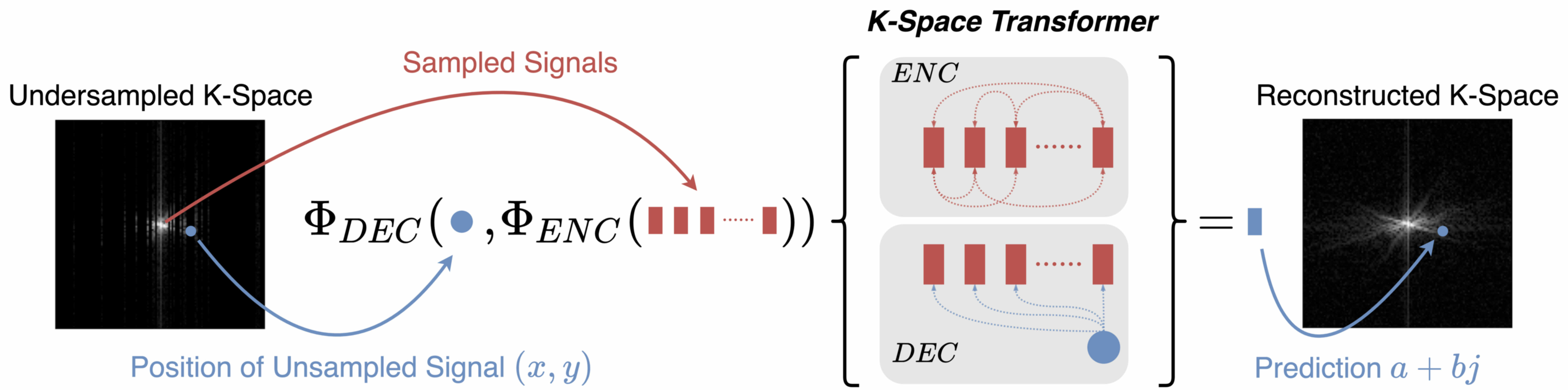
Figure 1: We adopt a transformer for implicit representation of k-space spectrogram (termed as K-Space Transformer).

In this paper, we propose a novel Transformer-based architecture for MRI reconstruction, termed as K-Space Transformer, that enables to learn inductive bias in k-space, as shown in Figure 1. Inspired by the implicit representation [Chen et al.(2021)Chen, Liu, and Wang, Mildenhall et al.(2020)Mildenhall, Srinivasan, Tancik, Barron, Ramamoorthi, and Ng], we treat the coordinates of unsampled k-space points as inputs to the Transformer Decoder, iteratively query information from those sampled points, and model relationships between any frequency bins beyond the regular spatial grids. Thanks to the high flexibility of such representation, we design a hierarchical decoder with coarse-to-fine reconstruction strategy, to strike a balance between performance and computational cost. Since pure k-space reconstruction would ignore important spatial bias in MRI, we further introduce an image domain refinement module to solve this problem. To summarise, our main contributions are three-fold:

• We introduce a novel hierarchical transformer architecture that aims to learn suitable inductive bias for directly processing signal in k-space. To the best of our knowledge, we are the first to introduce transformer to k-space reconstruction.

• We integrate image domain refinement module into the transformer decoder, and prove it to be complementary to the pure k-space reconstruction.

• We validate K-Space Transformer on two public datasets, demonstrating comparable or superior performance than previous state-of-the-art approaches.

2 Related Work

Undersampled MRI Reconstruction

is an ill-posed inverse problem. Based on the low dimensionality prior, traditional CS-Based methods generally leverage sparsity regularization in certain domain to reconstruct the image in iterative ways [Lustig et al.(2007)Lustig, Donoho, and Pauly]. However, the iterative optimization process often suffers from heavy parameter tuning [Yu et al.(2017)Yu, Dong, Yang, Slabaugh, Dragotti, Ye, Liu, Arridge, Keegan, Firmin, et al.] and long processing time [Hollingsworth(2015)]. Some works extend these approaches by construct deep networks to replace handcrafted parameters or functions [Yang et al.(2018)Yang, Sun, Li, and Xu, Zhang and Ghanem(2018)]. Another popular school of thought uses deep networks to learn a direct mapping from input to output [Han et al.(2019)Han, Sunwoo, and Ye, Du et al.(2021)Du, Zhang, Li, Pickup, Rosen, Zhou, Song, and Fan, Eo et al.(2018)Eo, Jun, Kim, Jang, Lee, and Hwang, Souza et al.(2019)Souza, Lebel, and Frayne, Zhou and Zhou(2020), Nitski et al.(2020)Nitski, Nag, McIntosh, and Wang, Lee et al.(2017)Lee, Yoo, and Ye, Schlemper et al.(2017)Schlemper, Caballero, Hajnal, Price, and Rueckert, Yang et al.(2017)Yang, Yu, Dong, Slabaugh, Dragotti, Ye, Liu, Arridge, Keegan, Guo, et al., Guo et al.(2021)Guo, Valanarasu, Wang, Zhou, Jiang, and Patel]. Most of these works focus on image domain reconstruction. For example, Schlemper et al. [Schlemper et al.(2017)Schlemper, Caballero, Hajnal, Price, and Rueckert] view the problem as image de-aliasing and propose a deep cascade framework of CNNs. Works in this direction have exploited various network architectures, including U-Net [Lee et al.(2017)Lee, Yoo, and Ye], GAN [Yang et al.(2017)Yang, Yu, Dong, Slabaugh, Dragotti, Ye, Liu, Arridge, Keegan, Guo, et al., Mardani et al.(2018)Mardani, Gong, Cheng, Vasanawala, Zaharchuk, Xing, and Pauly], convolutional RNN [Guo et al.(2021)Guo, Valanarasu, Wang, Zhou, Jiang, and Patel], Transformer [Huang et al.(2022)Huang, Fang, Wu, Wu, Gao, Li, Del Ser, Xia, and Yang] etc. Zhu et al. [Zhu et al.(2018)Zhu, Liu, Cauley, Rosen, and Rosen] propose to learn a mapping from k-space to image domain through fully connected layers, followed by convolutional layers. By contrast, Han et al. [Han et al.(2019)Han, Sunwoo, and Ye] use U-Net for direct k-space interpolation, complete the reconstruction purely in k-space. Du et al. [Du et al.(2021)Du, Zhang, Li, Pickup, Rosen, Zhou, Song, and Fan] further integrate channel and spatial attention mechanism into k-space convolution. Dual domain reconstruction is another natural choice to combine knowledge from both image domain and k-space [Eo et al.(2018)Eo, Jun, Kim, Jang, Lee, and Hwang, Souza et al.(2019)Souza, Lebel, and Frayne, Zhou and Zhou(2020), Nitski et al.(2020)Nitski, Nag, McIntosh, and Wang]. While k-space knowledge is commonly considered, the works so far base k-space learning on CNNs.

Implicit Neural Representation

parameterizes signals as continuous functions with neural networks, mapping coordinates to values. It have been widely applied to 3D object and scene modelling [Chen and Zhang(2019), Atzmon and Lipman(2020), Eslami et al.(2018)Eslami, Jimenez Rezende, Besse, Viola, Morcos, Garnelo, Ruderman, Rusu, Danihelka, Gregor, et al., Jiang et al.(2020)Jiang, Sud, Makadia, Huang, Nießner, Funkhouser, et al., Sitzmann et al.(2019)Sitzmann, Zollhöfer, and Wetzstein, Mildenhall et al.(2020)Mildenhall, Srinivasan, Tancik, Barron, Ramamoorthi, and Ng], and image processing [Karras et al.(2021)Karras, Aittala, Laine, Härkönen, Hellsten, Lehtinen, and Aila, Shaham et al.(2021)Shaham, Gharbi, Zhang, Shechtman, and Michaeli, Chen et al.(2021)Chen, Liu, and Wang]. However, its potential in medical image reconstruction is relatively less exploited. Wu et al. [Wu et al.(2021)Wu, Li, Xu, Feng, Wei, Yang, Yu, Liu, Yu, and Zhang] learn continuous volumeric function from discrete MRI slices to reconstruct high resolution 3D images. Shen et al. [Shen et al.(2022)Shen, Pauly, and Xing] takes a similar strategy but further embed prior image information into the network. Another related study [Sun et al.(2021)Sun, Liu, Xie, Wohlberg, and Kamilov] uses MLP to represent the measurement field of a CT image, and reconstruct from the generated measurements. Our work differs from the above mentioned works, as we share the function space across different instances, instead of optimizing unique representation for each individual object, and thus learn general prior knowledge of k-space.

3 Method

In this paper, we consider the problem of undersampled MRI reconstruction, with the goal of learning a function that maps the under-sampled spectrogram to high-quality MR images, $\mathcal{I}=\mathrm{\Phi}(x_{s};\Theta)$, where $\mathcal{I},x_{s}$ refers to the output MR image, and the input under-sampled spectrogram respectively, $\Theta$ denotes the set of learnable parameters.

Unlike existing work on MRI reconstruction that generally exploit ConvNets in image or k-space, we adopt the implicit representation, and propose a novel Transformer-based architecture for learning the inductive bias in k-space. In the following sections, we start by introducing the fundamental building blocks, namely, the Encoder module ($\Phi_{\text{ENC}}$) that learns a compact feature representation from sampled k-space points; and Decoder module ($\Phi_{\text{DEC}}$) that reconstructs MRI by alternating k-space decoding and image domain refinement. After that, we describe in detail how these blocks are used for constructing an hierarchical model, that strikes a balance on the performance and computational complexity trade-off.

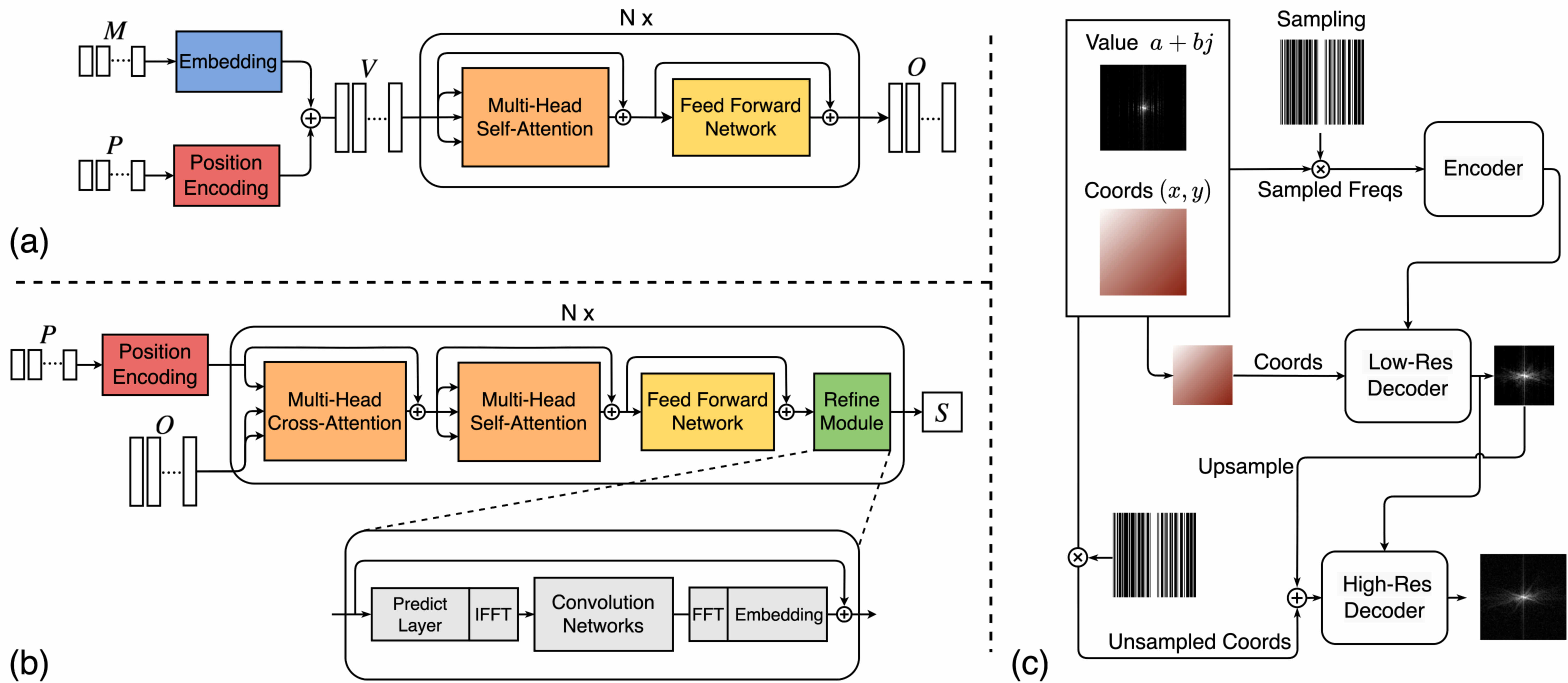
Figure 2: (a) The structure of Encoder; (b) The structure of Decoder; (c) The overall framework of the K-Space Transformer.

3.1 Feature Encoder

Here, the goal is to compute a compact feature representation for the sampled points in k-space. In detail, given a set of $n$ sampled points on spectrogram, i.e. $\{s_{i},\dots,s_{n}\}$, with $s_{i}=(m_{i},p_{i})$ refers to a combination of sampled complex value ($m_{i}\in\mathbb{R}^{2}$) and 2D spatial positions ($p_{i}\in\mathbb{R}^{2}$). Note that, $n$ is usually a small subset of all points on a spectrogram ($\mathbb{R}^{W\times H}$). As a tokenisation procedure that converts the sampled points into a vector sequence, $\mathcal{V}=\{v_{1},v_{2},\dots,v_{n}\}\in\mathbb{R}^{n\times d}$, with

$$v_{i}=\mathrm{\Phi}_{\textsc{Tokenize}}(s_{i})=\text{MLPs}(m_{i})+\text{PE}(p_{i})$$ (1)

where one Multilayer Perceptrons (MLPs) layer is applied to the sampled value, and PE refers to positional encodings with sine and cosine functions.

As shown in Figure 2 (a), the Encoder includes multiple standard transformer encoder layers, consisting of a multi-head self-attention module (MHSA), a feed forward network (FFN) and residual connections. Through self-attention module, the global dependency between each sampled point are captured, and the FFN further enriches the feature representation.

$$O=\mathrm{\Phi}_{\textsc{K-Enc}}(\mathcal{V})\in\mathbb{R}^{n\times d}$$ (2)

where $O$ denotes the output from encoder, with same dimensions as input sequence vectors. For more details, we would refer the readers to the original Transformer paper [Vaswani et al.(2017)Vaswani, Shazeer, Parmar, Uszkoreit, Jones, Gomez, Kaiser, and Polosukhin].

3.2 Feature Decoder

In this section, we describe the decoding procedure that maps the encoded representation to MR images. We adopt an hybrid architecture that alternates between k-space decoding, and refinement in image domain, shown in Figure 2 (b).

Decoding in k-space.

We adopt standard Transformer decoder layers, where the Key and Value are generated by applying two different linear transformations on encoder’s outputs, and the normalised positional coordinates for desired output ($\mathbb{R}^{W\times H}$) are encoded as Query:

$$q_{i}=W^{q}\cdot\text{PE}(p_{i})\text{\hskip 10.0pt}\forall p_{i}\in\mathbb{R}^{WH\times 2}$$ (3)

$$k_{i},\text{\hskip 5.0pt}v_{i}=W^{k}\cdot O_{i},\text{\hskip 5.0pt}W^{v}\cdot O_{i}\text{\hskip 10.0pt}\forall i\in[1,n]$$ (4)

$$S=g(\Phi_{\textsc{K-Dec}}(Q,K,V))\in\mathbb{R}^{W\times H\times 2}$$ (5)

where PE refers to positional encodings with sine and cosine functions, $q_{i},k_{i},v_{i}$ refer to $i$-th vector of $Q,K,V$ respectively, and $S$ denotes the predicted spectrogram by applying a linear MLP layer ($g(\cdot)$) on the output from transformer decoders ($\Phi_{\textsc{K-Dec}}(\cdot)$), consisting of multi-head self-attention (MHSA), multi-head cross-attention (MHCA), a feed-forward network (FFN), and residual connections. Note that, the resolution of the reconstructed spectrogram can be controlled by granularity of query, i.e. the number of positional coordinates.

Thanks to the flexibility of Transformer decoder layers, dependencies between all points on spectrogram can be effectively captured, thus enable to learn the inductive bias in k-space. However, one issue is, the point-wise update in k-space will globally affects all pixels in image domain, disregarding the spatial bias in MRI, that is, structures tend to be roughly aligned. To resolve such issue, we alternate the processing in k-space and image domain.

Refinement in Image Domain.

Here, we convert the reconstructed spectrogram into image domain with differentiable inverse Fast Fourier Transformer (FFT), and process the images with standard convolution layers ($\Phi_{\textsc{Img-Refine}}(\cdot)$):

$$\hat{S}=\mathcal{T}(\Phi_{\textsc{Img-Refine}}(\mathcal{T}^{-1}(S)))$$ (6)

where $\mathcal{T}$ and $\mathcal{T}^{-1}$ refer to FFT and inverse FFT respectively, the output is $\hat{S}\in\mathbb{R}^{W\times H\times 2}$.

Discussion:

At an high level, instead of treating the spectrogram as a look-up table array, i.e. values on regular grids, we adopt the implicit representation, learning a continuous function that maps the input positional coordinates to values, conditioned on the visible k-space samples. Such representation is highly flexible, as it not only enables to explicitly model the dependencies between different frequency bins, but also support to output spectrogram of different resolutions by simply varying the density of query coordinates.

3.3 Hierarchical Decoder

With the basic building blocks introduced, we construct an hierarchical decoder, to strike a balance between the computational cost and performance trade-off. In particular, we adopt a low-resolution (LR) decoder and a high-resolution (HR) decoder to guide the reconstruction with progressive resolutions, and tailor them for different purposes: $\mathrm{\Phi}_{\text{DEC}}(\cdot)=\mathrm{\Phi}_{\text{HRD}}\circ\mathrm{\Phi}_{\text{LRD}}(\cdot)$, where $\mathrm{\Phi}_{\text{LRD}}$ aims to reconstruct the spectrogram on a lower resolution, focusing on the overall anatomical structure. As shown in Figure 2 (c), this is simply implemented by adapting the normalised positional coordinate $p_{i}$ in Equation 3 to a down-sampled spectrogram. Here, we do not use image domain refinement, and only implement the LR decoder with standard Transformer decoder layers.

The HR decoder aims to fill the texture details based on the LR output. We accordingly map the tokenised HR coordinates (Eq. 3) to queries, and treat the two projections of LR decoder output as Key and Value. To alleviate the computation from self-attention module, we simplify each decoder layer in HR decoder with only cross-attention module left.

Discussion:

As for computational complexity, when decoding the $m$-length sequence from the $n$-length sampled points with a standard Transformer decoder, the complexity would be $\mathcal{O}(mn)$ for MHCA and $\mathcal{O}(m^{2})$ for MHSA, which is prohibitively expensive when $m$ is very large. However, in our case, by constructing the hierarchical model, the computation complexity is reduced to $\mathcal{O}(ml+nl+l^{2})$, as the MHSA can simply be done in LR decoder, drastically cutting the memory consumption, when $l$ is set to be much smaller than $m$.

4 Experiment

4.1 Dataset & Metrics

We employ two datasets for evaluation, namely, OASIS and fastMRI. OASIS [Marcus et al.(2007)Marcus, Wang, Parker, Csernansky, Morris, and Buckner] contains 3,398 single-coil T1-weighted brain MRI volumes, each has 175 slices. We split them into train and test sets with ratio 3:1 and uniformly draw 10% from them. Additionally, fastMRI has 1172 single-coil PD-weighted knee MRI volumes, each includes 35 slices. We use 973 for training, 199 for testing and uniformly draw 25% slices from both. Following conventional evaluation, we experiment on five undersampling settings: Gaussian 2D sampling with 10$\times$, 5$\times$ and $2.5\times$ accelerations; Uniform 1D sampling with 5$\times$ and $2.5\times$ accelerations. Peak signal to noise ratio (PSNR) and structural index similarity (SSIM) are used as metrics.

4.2 Comparison to State-of-the-art

We compare to 6 representative methods, including UNet [Ronneberger et al.(2015)Ronneberger, Fischer, and Brox] for image domain reconstruction and k-space reconstruction, Deep ADMM Net [Yang et al.(2018)Yang, Sun, Li, and Xu], D5C5 [Schlemper et al.(2017)Schlemper, Caballero, Hajnal, Price, and Rueckert], SwinMR[Huang et al.(2022)Huang, Fang, Wu, Wu, Gao, Li, Del Ser, Xia, and Yang] and previous state-of-the-art OUCR [Guo et al.(2021)Guo, Valanarasu, Wang, Zhou, Jiang, and Patel]. For implementation details of K-Space Transformer and the baseline methods, please refer to the supplementary details.

Quantitative Results:

As shown in Table 1, our method achieves the best results under all 1D settings. On OASIS, we improved the PSNR from 29.52 dB to 31.50 dB with 5$\times$ acceleration, and for 2.5$\times$ sampling, our improvement is even enlarged to 2.57 dB. On fastMRI, we outperform the best baseline slightly, however we also notice that the top approaches perform quite closely, we conjecture this is because the dataset is quite noisy, which may lead to an unprecise supervision for training and evaluation. In addition, it’s noticeable that K-UNet leads to poorer performance compared with UNet, showing that naïve CNN-based methods do not give suitable inductive bias for k-space reconstruction. On 2D settings (Table 2), our method either outperforms or achieve competitive results to the state-of-the-part approaches.

Method	OASIS				fastMRI
	5 $\times$		2.5 $\times$		5 $\times$		2.5 $\times$
	PSNR	SSIM	PSNR	SSIM	PSNR	SSIM	PSNR	SSIM
K-UNet	24.53	0.7808	26.50	0.8483	24.68	0.6058	26.99	0.7223
Deep ADMM	26.03	0.7202	29.95	0.8165	24.43	0.6172	29.84	0.7838
SwinMR	27.17	0.9041	29.83	0.9435	26.01	0.6684	29.10	0.7842
UNet	27.53	0.8895	29.05	0.8988	26.72	0.6835	29.81	0.7983
D5C5	27.66	0.8895	32.48	0.9615	26.87	0.6793	30.64	0.8126
OUCR	29.52	0.9310	33.75	0.9709	27.71	0.7009	30.95	0.8168
Ours	31.50	0.9528	36.32	0.9848	27.80	0.7078	31.04	0.8189

Table 1: Quantitative comparison on uniform 1D sampling settings.

Method	OASIS						fastMRI
	10 $\times$		5 $\times$		2.5 $\times$		5 $\times$		2.5 $\times$
	PSNR	SSIM	PSNR	SSIM	PSNR	SSIM	PSNR	SSIM	PSNR	SSIM
K-UNet	25.34	0.766	28.76	0.8427	33.96	0.9288	27.15	0.6696	28.90	0.7710
Deep ADMM	26.17	0.7312	30.41	0.8122	33.94	0.8513	29.31	0.7515	30.97	0.8162
SwinMR	27.48	0.8893	30.36	0.9341	33.75	0.9659	28.41	0.7080	30.30	0.7949
UNet	27.63	0.8437	31.27	0.9024	35.02	0.9388	28.33	0.7120	31.35	0.8283
D5C5	30.51	0.9241	35.91	0.9743	42.72	0.9927	29.78	0.7507	32.00	0.8399
OUCR	31.61	0.9442	36.78	0.9797	42.80	0.9933	29.95	0.7522	32.04	0.8382
Ours	32.58	0.9529	37.47	0.9823	43.68	0.9946	29.88	0.7534	31.97	0.8389

Table 2: Quantitative comparison on Gaussian 2D sampling settings.

Qualitative Results:

In Figure 3, we show some predictions from K-Space Transformer on 5$\times$ uniform sampling setting. On OASIS, our method clearly retain more texture information and less structural loss compared with others, suggesting that our method is more robust for such severe distortion in image domain. While on fastMRI, the groundtruth images are often noisy, which might explain why the top approaches perform similarly. Due to space limit, we attach more qualitative comparison results in the supplementary material.

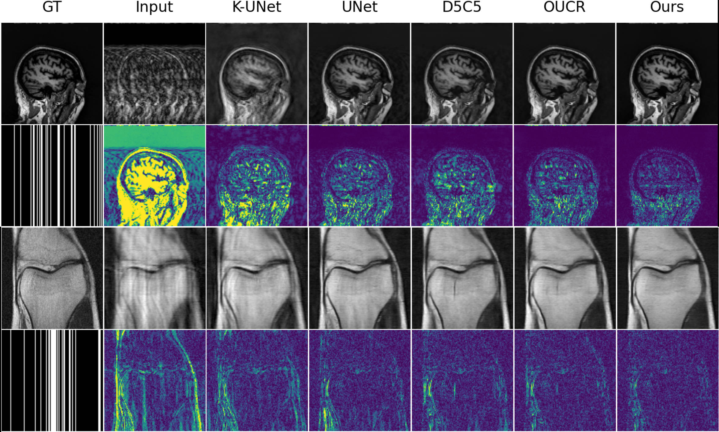
Figure 3: Qualitative comparison under 5$\times$ uniform sampling setting. The even-numbered rows show the sampling trajectories and error maps, where brighter means higher error.

4.3 Ablation Study

To investigate the effectiveness of hybrid learning and the hierarchical structure, we remove the image domain refinement module (RM), and the LR decoder (LRD) sequentially on OASIS dataset.

As shown in Table 3, without the refinement module, the reconstruction quality drops significantly, showing the image domain refinement can indeed provide supplementary information for k-space reconstruction. Nevertheless, our method still achieves competitive

Modules		Gaussian 2D 5$\times$		Uniform 1D 5$\times$
LRD	RM	PSNR	SSIM	PSNR	SSIM
✓	✓	37.47	0.9823	31.50	0.9528
✓	✗	32.97	0.9337	27.52	0.8876
✗	✗	28.53	0.8416	21.31	0.6114

Table 3: Quantitive ablation study on critical designs.

results and outperforms K-UNet by a large margin (refer to Table 1 and 2), which justifies Transformer’s superiority for k-space reconstruction. In addition, removing the LR decoder further leads to an obvious performance degradation, implying that our hierarchical design also plays an essential role in guaranteeing an excellent reconstruction quality with a moderate computational cost.

To give a more distinct illustration, we further visualize some intermediate results of K-Space Transformer in Figure 4. We observe the LR decoder capable to reconstruct a basic outline of the structure, equally the low-mid frequency bands of the spectrogram. Based on the upsampled rough result, the HR decoder fills in the texture details, i.e., completing higher frequency bands. The coarse-to-fine progress is consistent with our assumption in Section 3.3. Compared to standard HR decoder, those without refinement module contain more noise over the structures and background, which is easier to remove via spatial convolution. It indicates the inductive bias of image domain are complementary to k-space.

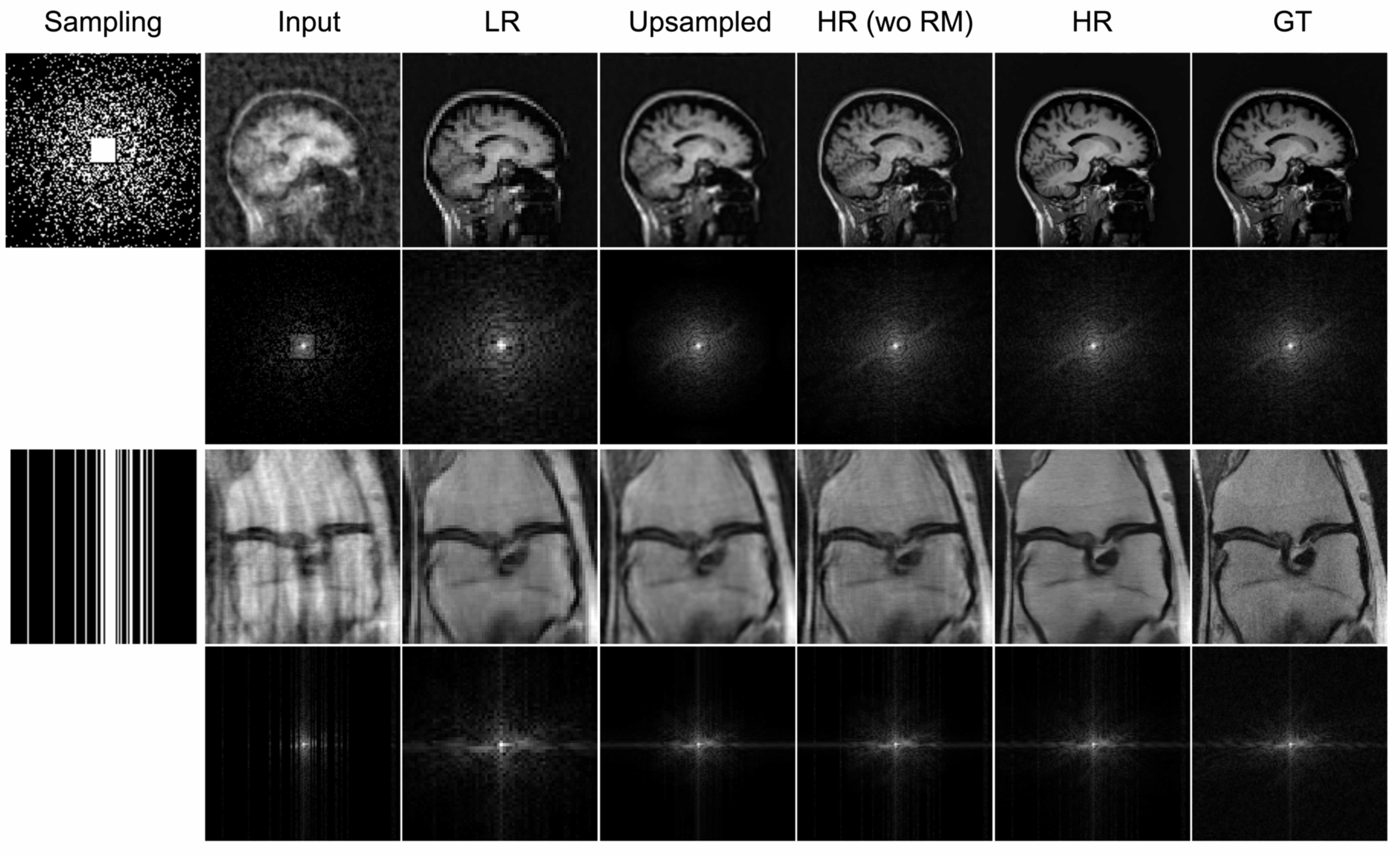
Figure 4: Intermediate results of K-Space Transformer: LR denotes the reconstruction output of LR decoder; Upsampled denotes the up-sampled result; HR and HR (wo RM) refer to the output of HR decoder and that without refinement module.

On Positional Encoding and Receptive Field.

To make comparison between UNet and Transformer, we also extend the standard U-Net with additional positional encoding and large receptive field (more parameters). By explicitly concatenate the postional encodings with k-space spectrogram as the input, we change the convolution into position dependent (denoted as U-Net P); We further enlarge the receptive filed by adopting $5\times 5$ kernel and deeper convolution layers (denoted as K U-Net P L).

As shown in Table 4, both positional encoding and large receptive field improve the performance of a standard U-Net. However, the gain is marginal, note that a large receptive field would increase the model size exponentially.

Method	OASIS				fastMRI
	Uniform		Gaussian		Uniform		Gaussian
	5$\times$	2.5$\times$	5$\times$	2.5$\times$	5$\times$	2.5$\times$	5$\times$	2.5$\times$
K U-Net	24.53	26.50	28.76	33.96	24.68	26.99	27.15	28.90
K U-Net P	24.55	26.67	29.18	35.10	24.70	28.13	27.56	29.98
K U-Net P L	24.64	27.00	29.87	35.18	24.71	28.44	27.68	30.01
Ours	31.50	36.32	37.47	43.68	27.80	31.04	29.88	31.97

Table 4: Comparision between U-Net variants and Transformer (PSNR).

4.4 Visualising Transformer in K-Space Learning

Here, we visualize the attention maps of our encoder and decoder according to, i.e., $\text{attn}=\text{softmax}(QK^{T}/\sqrt{d})$, where $Q$ and $K$ refer to the Query and Key indicated in section 3.1 and 3.2. Recall that we expect the K-Space Transformer to fully exploit the relationship between any points for reconstruction. As shown in Figure 5, we do observe both the global and local interactions have been well exploited through the attention mechanism, as there are some heads clearly scanning the spectrogram globally, and others focusing on specific regions of interests, implying that the model can indeed capture inductive bias in k-space.

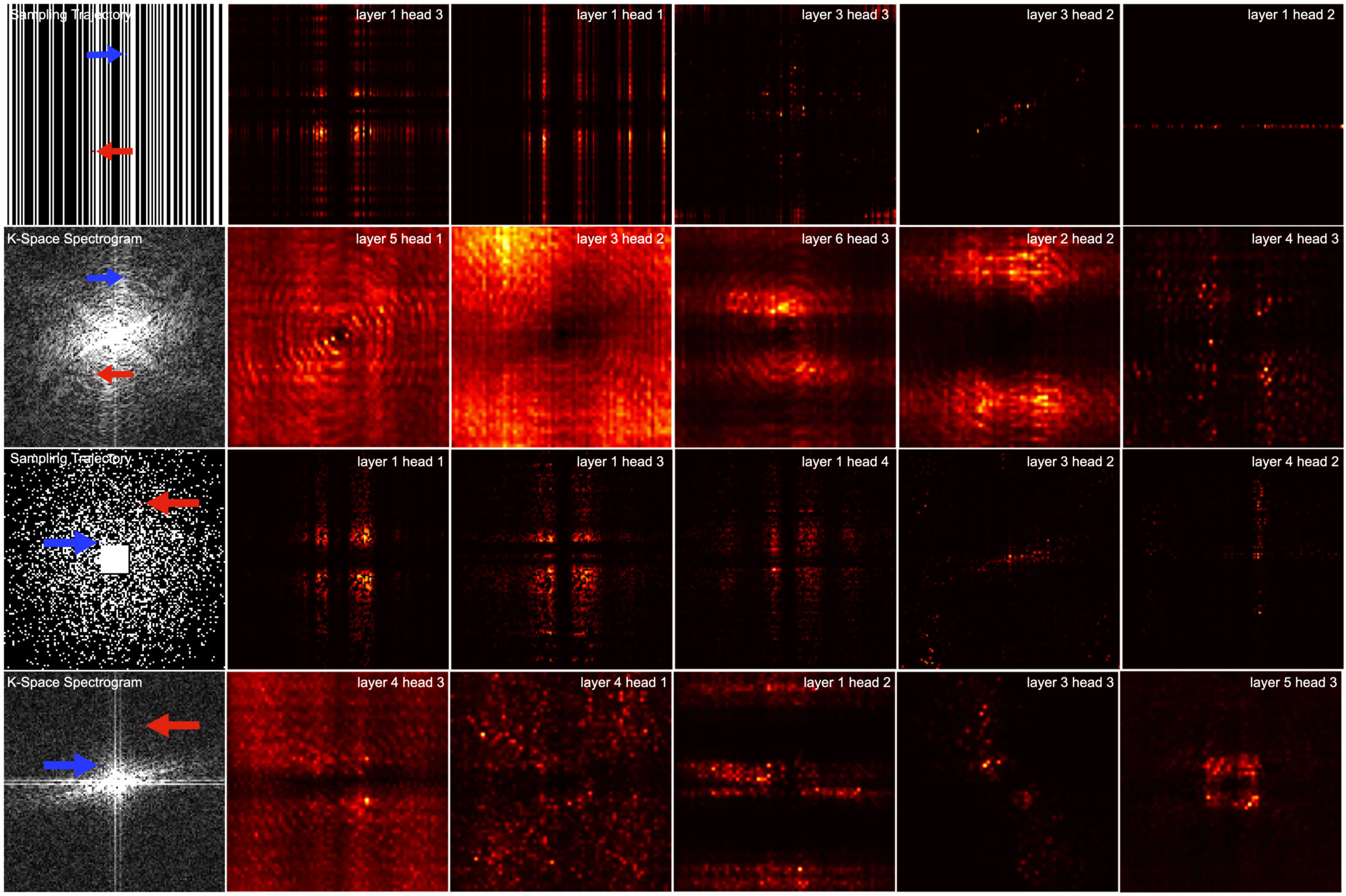
Figure 5: Attention maps from the encoder and decoder under different sampling patterns. We randomly select a sampled point (indicated by the red arrow) and visualize its attention map in encoder in the upper rows (i.e. relationship with other sampled points); We randomly select a unsampled point(the blue arrow) and visualize its attention map in HR decoder in the lower rows (i.e. relationship with the reconstructed LR spectrogram).

5 Conclusion

We propose K-Space Transformer, a novel Transformer-based architecture for undersampled MRI reconstruction. It exploits implicit representation, and learns the global dependencies between frequency bins in k-space. Specifically, we design a flexible hierarchical decoder to produce high quality reconstruction with moderate computational cost. Extensive experiments show that the proposed K-Space Transformer outperforms existing state-of-the-art methods or achieves comparable performance on two public datasets, demonstrating promising results of Transformer in MRI reconstruction and k-space learning. Future studies can be conducted to adapt it to multi-coil imaging, k-space super-resolution and other potentially relevant directions.

In this supplementary mateirial, we start by introducing implement details on the proposed K-Space Transformer and baseline methods included in our experiments. Then, we demonstrate ablation study on the influence of a deeper K-Space Transformer and how the hybrid learning works in the HR Decoder. Finally, we supplement more qualitative comparison results on settings that are not included in Section 4.2 .

6 Implement Details

K-Space Transformer is implemented with 4 Encoder layers, 4 Low-Resolution Decoder layers and 6 High-Resolution Decoder layers. Each encoder layer is equipped with a four-head self-attention layer and a feed forward network; each LR decoder layer is equipped with a four-head cross-attention layer, a four-head self-attention layer and a feed forward network; and each HR decoder layer is equipped with a four-head cross-attention, a feed forward network and a refinement module. The backone of refinement module consists of 5 convolution layers with leaky ReLU activations between. The first four layers has 64 filters of 3$\times$3 kernel; while the last layer has 2 filters of 3$\times$3 kernel. Necessary prediction, embedding and fft/ifft layers are inserted before and after the convolutions for transformation between k-space and image domain. By default, the embedding layers, prediction layers and feed forward networks mentioned in this paper are two-level MLPs with ReLu activations between. Following previous works [Du et al.(2021)Du, Zhang, Li, Pickup, Rosen, Zhou, Song, and Fan, Guo et al.(2021)Guo, Valanarasu, Wang, Zhou, Jiang, and Patel, Han et al.(2019)Han, Sunwoo, and Ye, Schlemper et al.(2017)Schlemper, Caballero, Hajnal, Price, and Rueckert, Souza et al.(2019)Souza, Lebel, and Frayne], we treat the input and output complex MR signals as double channels, i.e., real and imaginary. Features vectores and 2D positional encodings mentioned in Section 3 are set with the same dimensionality $d=256$.

We adopt pixel-wise loss between reconstruction $\mathcal{I}$ and groundtruth $\mathcal{I}_{gt}$ in image domain, and apply deep supervision [Lee et al.(2015)Lee, Xie, Gallagher, Zhang, and Tu] on each layer of LR and HR decoders : $\mathcal{L}=\sum_{i}\|\mathcal{I}_{i}-\mathcal{I}_{gt}\|_{2}$, where $i$ indicates the layer depth. We train K-Space Transformer with AdamW optimizer and cosine annealing schedule, setting the initial learning rate as $5\times 10^{-4}$. Inspired by  [Xiong et al.(2020)Xiong, Yang, He, Zheng, Zheng, Xing, Zhang, Lan, Wang, and Liu], we adopt Pre-LN architecture to save warm-up stage. As the HR reconstruction depends on the LR decoder output (refer to Section 3.3), we find it helpful to stop the gradients from HR decoder outputs in early epochs, i.e., only update the LR decoder. Training is conducted on 4 RTX 3090.

Other Baseline Approaches. We implement a standard U-Net [Ronneberger et al.(2015)Ronneberger, Fischer, and Brox] with data consistency layer before the final output for U-Net and K U-Net, which follows the same architecture as  [Han et al.(2019)Han, Sunwoo, and Ye]. We train the network with the same objective function and learning rate as our methods but adopt an Adam optimizer. We implement D5C5 [Schlemper et al.(2017)Schlemper, Caballero, Hajnal, Price, and Rueckert] according to its official configuration for 2D images reconstruction: a cascade network of 5 CNNs, each equipped with 5 layers and a data consistency layer. We train it with the same hyper-parameters as U-Net. For Deep ADMM [Yang et al.(2018)Yang, Sun, Li, and Xu], SwinMR [Huang et al.(2022)Huang, Fang, Wu, Wu, Gao, Li, Del Ser, Xia, and Yang] and OUCR [Guo et al.(2021)Guo, Valanarasu, Wang, Zhou, Jiang, and Patel], we adopt their official source codes and default hyper-parameters that are publicly available or provided by the authors.

7 Influence of Network Depth

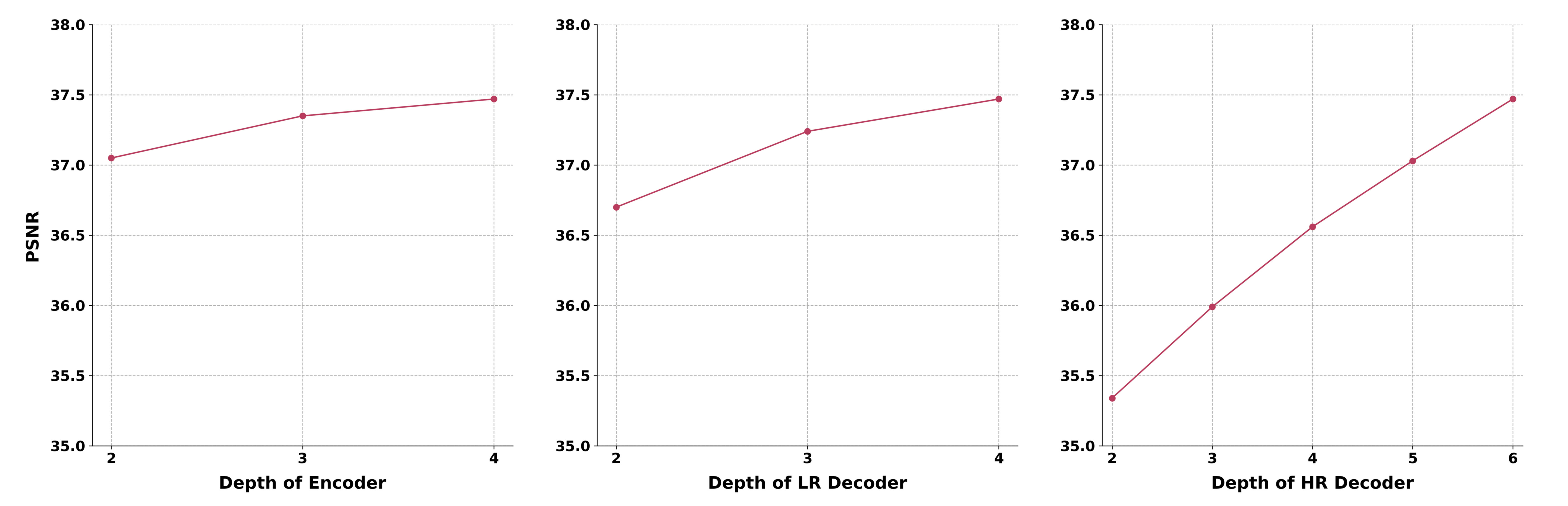
Figure 6: The performance influence of increasing module depth.

We investigate the effect of layer depth in K-Space Transformer by increasing the depth of Encoder, LR Decoder and HR Decoder respectively and evaluate under Gaussian sampling, 5x acceleration. As demonstrated in Figure 6, increasing depth consistently improve the network performance in all three modules. Though we conjecture our model may benefit from even deeper architecture, we take a default setting as 4 Encoder layers, 4 Low-Resolution Decoder layers and 6 High-Resolution Decoder layers to balance the computational cost.

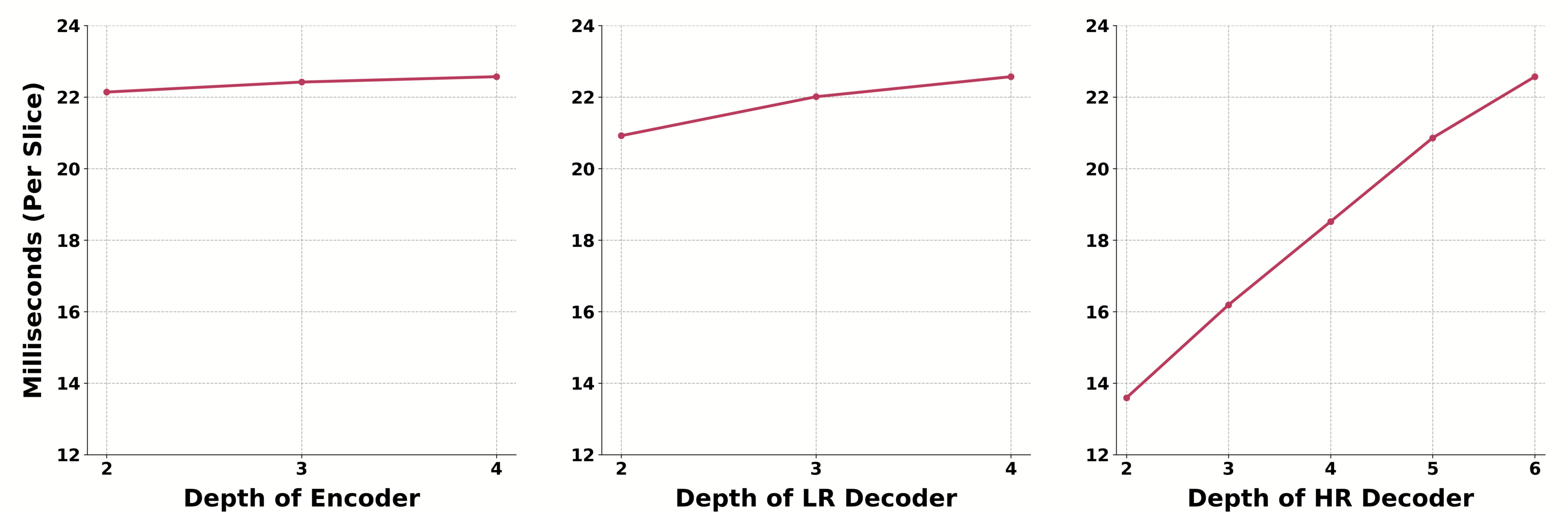
Figure 7: The speed influence of increasing module depth.

On Reconstruction Speed. Here, we evaluate the reconstruction time, as expected, deeper networks tend to incur longer processing time, shown in Figure 7. For example, depending on the depth of the HR decoder, the average inference time for each slice could range from 13.6ms to 22.6ms. By comparison, it’s significantly faster than Deep ADMM (around 1s) and traditional CS-based methods (up to hundreds of seconds) and comparable to SwinMR (around 18ms), and only slightly slower than the existing CNN-based methods (a few milliseconds). However, we believe the processing speed of our model is sufficient for real-time imaging, thus its remarkable performance improvement on high acceleration settings should be more valuable to improve the patients’ scanning experience and reduce medical cost in clinical application.

8 Effectiveness of Hybrid Learning

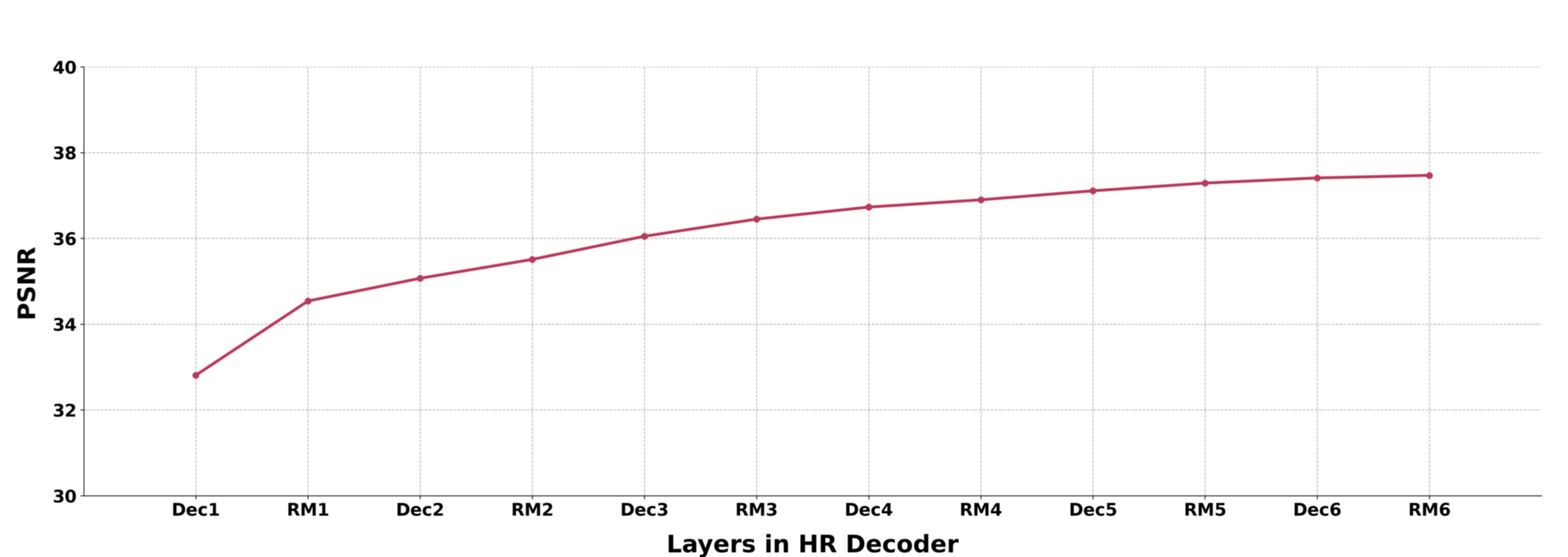
Figure 8: Evaluation on deep supervised reconstruction from each k-space decoding(denoted as Dec) and image refinement module(denoted as RM) in the HR Decoder.

We have shown that image domain refinement does provide complementary information to k-space decoding in Section 4.3 . Here, we further investigate how the alternating process works in the hybrid learning. After evaluating the deep supervised reconstructed results of each HR decoder layer under Gaussian sampling, 5x acceleration (shown in Figure 8), we observe that PSNR increases consistently throughout the alternation between k-space decoding and image domain refinement, and this finding is consistent across all the settings.

9 Supplementary Qualitative Comparison with Baselines

We show more qualitative comparisons that are not included in Section 4.2 . As can be seen from Figure 9 and Figure 10, on settings like 2.5x uniform sampling or 10x Gaussian sampling, our method achieve remarkably higher reconstruction quality over other approaches, demonstrating the robustness to more significant aliasing artifacts. While on settings with less structure loss and aliasing artifacts, the top methods perform quite close.

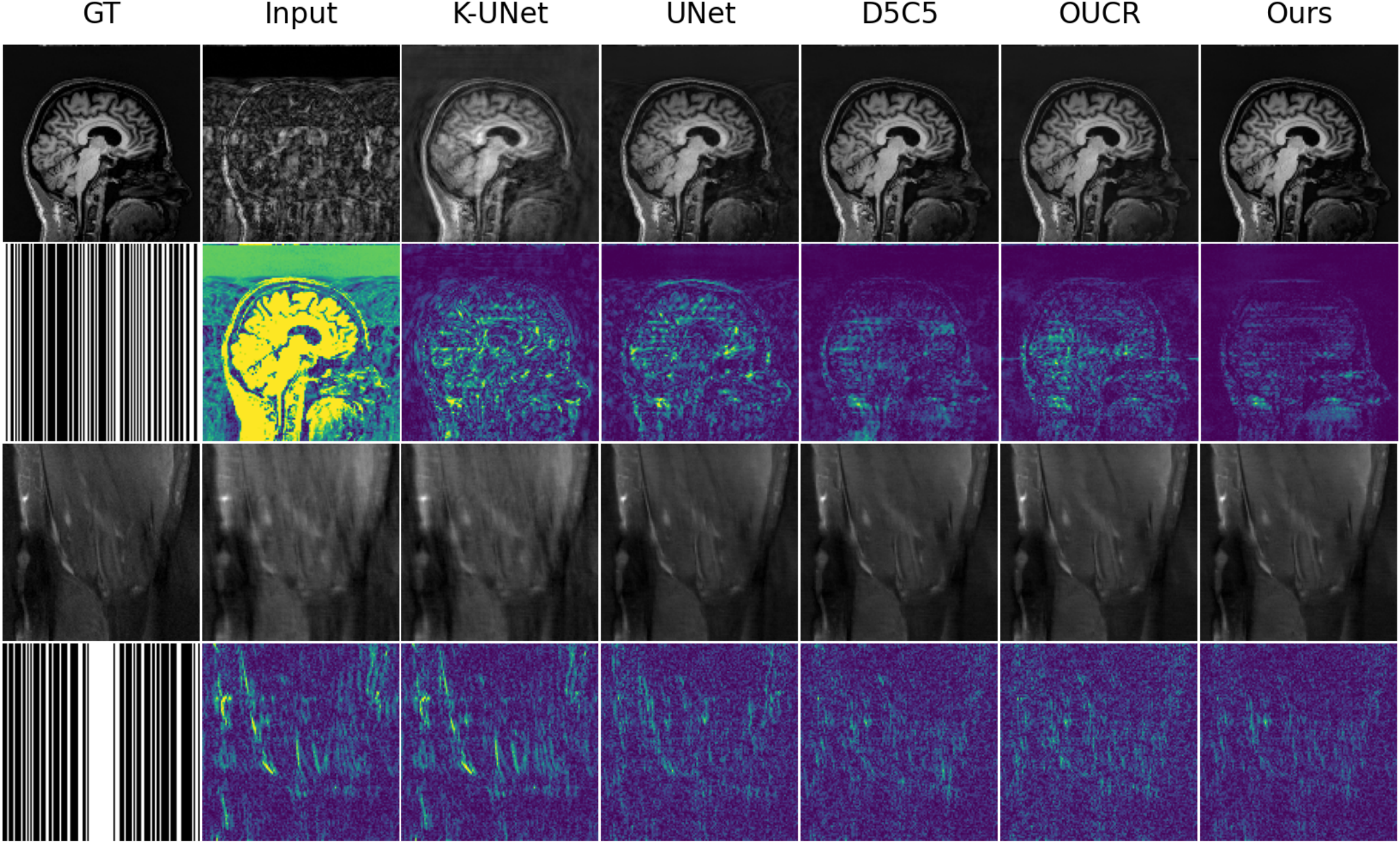
Figure 9: Supplementary qualitative comparison on uniform sampling settings.

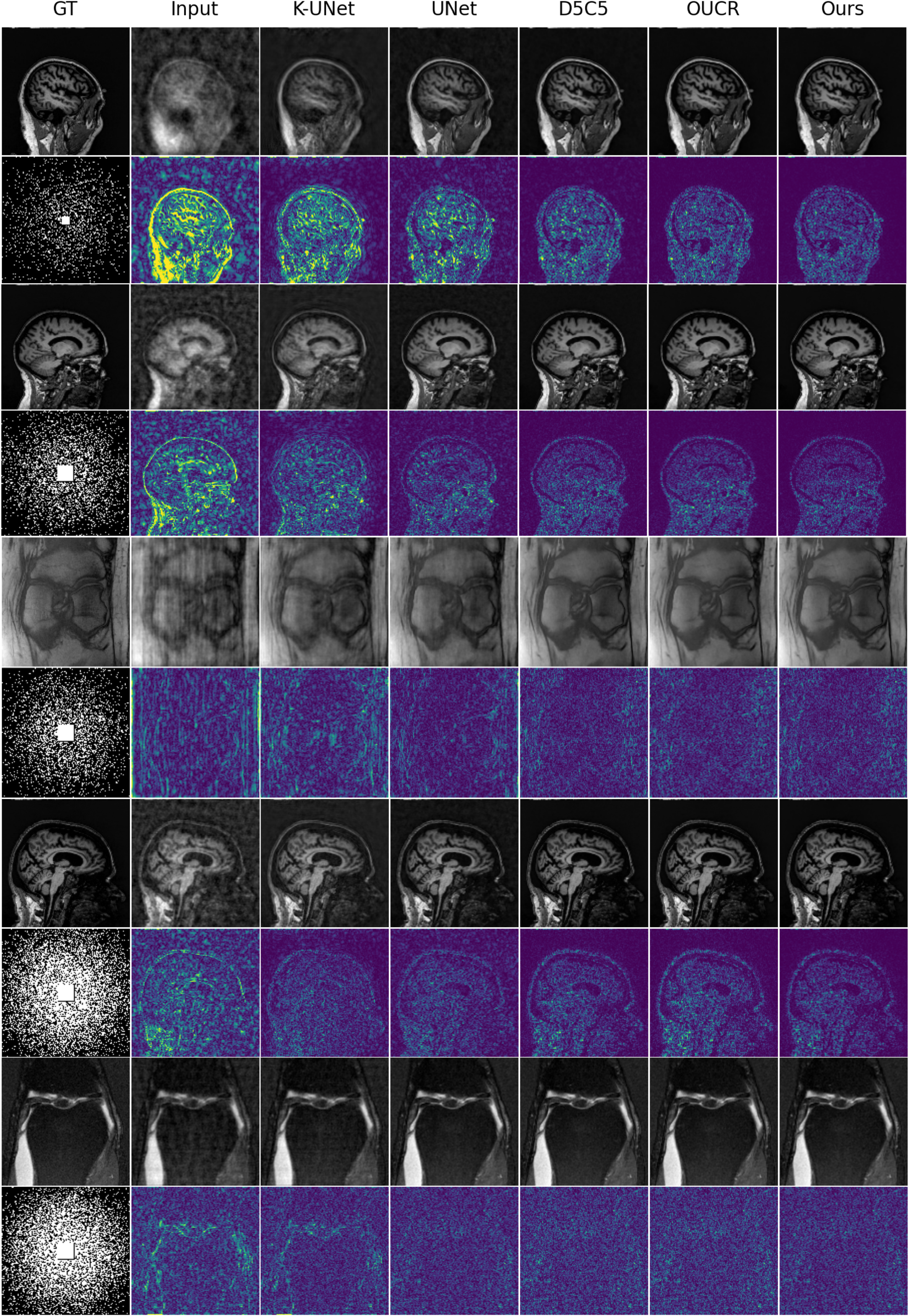
Figure 10: Supplementary qualitative comparison on Gaussian sampling settings.

References

- [Atzmon and Lipman(2020)] Matan Atzmon and Yaron Lipman. Sal: Sign agnostic learning of shapes from raw data. In IEEE/CVF Conference on Computer Vision and Pattern Recognition (CVPR), June 2020.
- [Chen et al.(2021)Chen, Liu, and Wang] Yinbo Chen, Sifei Liu, and Xiaolong Wang. Learning continuous image representation with local implicit image function. In Proceedings of the IEEE/CVF Conference on Computer Vision and Pattern Recognition, pages 8628–8638, 2021.
- [Chen and Zhang(2019)] Zhiqin Chen and Hao Zhang. Learning implicit fields for generative shape modeling. In Proceedings of the IEEE/CVF Conference on Computer Vision and Pattern Recognition (CVPR), June 2019.
- [Du et al.(2021)Du, Zhang, Li, Pickup, Rosen, Zhou, Song, and Fan] Tianming Du, Honggang Zhang, Yuemeng Li, Stephen Pickup, Mark Rosen, Rong Zhou, Hee Kwon Song, and Yong Fan. Adaptive convolutional neural networks for accelerating magnetic resonance imaging via k-space data interpolation. Medical Image Analysis, 72:102098, 2021.
- [Eo et al.(2018)Eo, Jun, Kim, Jang, Lee, and Hwang] Taejoon Eo, Yohan Jun, Taeseong Kim, Jinseong Jang, Ho-Joon Lee, and Dosik Hwang. Kiki-net: cross-domain convolutional neural networks for reconstructing undersampled magnetic resonance images. Magnetic resonance in medicine, 80(5):2188–2201, 2018.
- [Eslami et al.(2018)Eslami, Jimenez Rezende, Besse, Viola, Morcos, Garnelo, Ruderman, Rusu, Danihelka, Gregor, et al.] SM Ali Eslami, Danilo Jimenez Rezende, Frederic Besse, Fabio Viola, Ari S Morcos, Marta Garnelo, Avraham Ruderman, Andrei A Rusu, Ivo Danihelka, Karol Gregor, et al. Neural scene representation and rendering. Science, 360(6394):1204–1210, 2018.
- [Guo et al.(2021)Guo, Valanarasu, Wang, Zhou, Jiang, and Patel] Pengfei Guo, Jeya Maria Jose Valanarasu, Puyang Wang, Jinyuan Zhou, Shanshan Jiang, and Vishal M Patel. Over-and-under complete convolutional rnn for mri reconstruction. In International Conference on Medical Image Computing and Computer-Assisted Intervention, pages 13–23. Springer, 2021.
- [Han et al.(2019)Han, Sunwoo, and Ye] Yoseo Han, Leonard Sunwoo, and Jong Chul Ye. k-space deep learning for accelerated mri. IEEE transactions on medical imaging, 39(2):377–386, 2019.
- [Hollingsworth(2015)] Kieren Grant Hollingsworth. Reducing acquisition time in clinical mri by data undersampling and compressed sensing reconstruction. Physics in Medicine & Biology, 60(21):R297, 2015.
- [Huang et al.(2022)Huang, Fang, Wu, Wu, Gao, Li, Del Ser, Xia, and Yang] Jiahao Huang, Yingying Fang, Yinzhe Wu, Huanjun Wu, Zhifan Gao, Yang Li, Javier Del Ser, Jun Xia, and Guang Yang. Swin transformer for fast mri. Neurocomputing, 493:281–304, 2022.
- [Jiang et al.(2020)Jiang, Sud, Makadia, Huang, Nießner, Funkhouser, et al.] Chiyu Jiang, Avneesh Sud, Ameesh Makadia, Jingwei Huang, Matthias Nießner, Thomas Funkhouser, et al. Local implicit grid representations for 3d scenes. In Proceedings of the IEEE/CVF Conference on Computer Vision and Pattern Recognition, pages 6001–6010, 2020.
- [Karras et al.(2021)Karras, Aittala, Laine, Härkönen, Hellsten, Lehtinen, and Aila] Tero Karras, Miika Aittala, Samuli Laine, Erik Härkönen, Janne Hellsten, Jaakko Lehtinen, and Timo Aila. Alias-free generative adversarial networks. In Proc. NeurIPS, 2021.
- [Lee et al.(2015)Lee, Xie, Gallagher, Zhang, and Tu] Chen-Yu Lee, Saining Xie, Patrick Gallagher, Zhengyou Zhang, and Zhuowen Tu. Deeply-supervised nets. In Artificial intelligence and statistics, pages 562–570. PMLR, 2015.
- [Lee et al.(2017)Lee, Yoo, and Ye] Dongwook Lee, Jaejun Yoo, and Jong Chul Ye. Deep residual learning for compressed sensing mri. In 2017 IEEE 14th International Symposium on Biomedical Imaging (ISBI 2017), pages 15–18, 2017. 10.1109/ISBI.2017.7950457.
- [Lustig et al.(2007)Lustig, Donoho, and Pauly] Michael Lustig, David Donoho, and John M Pauly. Sparse mri: The application of compressed sensing for rapid mr imaging. Magnetic Resonance in Medicine: An Official Journal of the International Society for Magnetic Resonance in Medicine, 58(6):1182–1195, 2007.
- [Marcus et al.(2007)Marcus, Wang, Parker, Csernansky, Morris, and Buckner] Daniel S Marcus, Tracy H Wang, Jamie Parker, John G Csernansky, John C Morris, and Randy L Buckner. Open access series of imaging studies (oasis): cross-sectional mri data in young, middle aged, nondemented, and demented older adults. Journal of cognitive neuroscience, 19(9):1498–1507, 2007.
- [Mardani et al.(2018)Mardani, Gong, Cheng, Vasanawala, Zaharchuk, Xing, and Pauly] Morteza Mardani, Enhao Gong, Joseph Y Cheng, Shreyas S Vasanawala, Greg Zaharchuk, Lei Xing, and John M Pauly. Deep generative adversarial neural networks for compressive sensing mri. IEEE transactions on medical imaging, 38(1):167–179, 2018.
- [Mildenhall et al.(2020)Mildenhall, Srinivasan, Tancik, Barron, Ramamoorthi, and Ng] Ben Mildenhall, Pratul P Srinivasan, Matthew Tancik, Jonathan T Barron, Ravi Ramamoorthi, and Ren Ng. Nerf: Representing scenes as neural radiance fields for view synthesis. In European conference on computer vision, pages 405–421. Springer, 2020.
- [Nitski et al.(2020)Nitski, Nag, McIntosh, and Wang] Osvald Nitski, Sayan Nag, Chris McIntosh, and Bo Wang. Cdf-net: Cross-domain fusion network for accelerated mri reconstruction. In International Conference on Medical Image Computing and Computer-Assisted Intervention, pages 421–430. Springer, 2020.
- [Ronneberger et al.(2015)Ronneberger, Fischer, and Brox] Olaf Ronneberger, Philipp Fischer, and Thomas Brox. U-net: Convolutional networks for biomedical image segmentation. In International Conference on Medical image computing and computer-assisted intervention, pages 234–241. Springer, 2015.
- [Schlemper et al.(2017)Schlemper, Caballero, Hajnal, Price, and Rueckert] Jo Schlemper, Jose Caballero, Joseph V Hajnal, Anthony N Price, and Daniel Rueckert. A deep cascade of convolutional neural networks for dynamic mr image reconstruction. IEEE transactions on Medical Imaging, 37(2):491–503, 2017.
- [Shaham et al.(2021)Shaham, Gharbi, Zhang, Shechtman, and Michaeli] Tamar Rott Shaham, Michaël Gharbi, Richard Zhang, Eli Shechtman, and Tomer Michaeli. Spatially-adaptive pixelwise networks for fast image translation. In Proceedings of the IEEE/CVF Conference on Computer Vision and Pattern Recognition, pages 14882–14891, 2021.
- [Shen et al.(2022)Shen, Pauly, and Xing] Liyue Shen, John Pauly, and Lei Xing. Nerp: implicit neural representation learning with prior embedding for sparsely sampled image reconstruction. IEEE Transactions on Neural Networks and Learning Systems, 2022.
- [Sitzmann et al.(2019)Sitzmann, Zollhöfer, and Wetzstein] Vincent Sitzmann, Michael Zollhöfer, and Gordon Wetzstein. Scene representation networks: Continuous 3d-structure-aware neural scene representations. Advances in Neural Information Processing Systems, 32, 2019.
- [Souza et al.(2019)Souza, Lebel, and Frayne] Roberto Souza, R Marc Lebel, and Richard Frayne. A hybrid, dual domain, cascade of convolutional neural networks for magnetic resonance image reconstruction. In International Conference on Medical Imaging with Deep Learning, pages 437–446. PMLR, 2019.
- [Sun et al.(2021)Sun, Liu, Xie, Wohlberg, and Kamilov] Yu Sun, Jiaming Liu, Mingyang Xie, Brendt Wohlberg, and Ulugbek S Kamilov. Coil: Coordinate-based internal learning for imaging inverse problems. arXiv preprint arXiv:2102.05181, 2021.
- [Vaswani et al.(2017)Vaswani, Shazeer, Parmar, Uszkoreit, Jones, Gomez, Kaiser, and Polosukhin] Ashish Vaswani, Noam Shazeer, Niki Parmar, Jakob Uszkoreit, Llion Jones, Aidan N Gomez, Łukasz Kaiser, and Illia Polosukhin. Attention is all you need. Advances in neural information processing systems, 30, 2017.
- [Wu et al.(2021)Wu, Li, Xu, Feng, Wei, Yang, Yu, Liu, Yu, and Zhang] Qing Wu, Yuwei Li, Lan Xu, Ruiming Feng, Hongjiang Wei, Qing Yang, Boliang Yu, Xiaozhao Liu, Jingyi Yu, and Yuyao Zhang. Irem: High-resolution magnetic resonance image reconstruction via implicit neural representation. In International Conference on Medical Image Computing and Computer-Assisted Intervention, pages 65–74. Springer, 2021.
- [Xiong et al.(2020)Xiong, Yang, He, Zheng, Zheng, Xing, Zhang, Lan, Wang, and Liu] Ruibin Xiong, Yunchang Yang, Di He, Kai Zheng, Shuxin Zheng, Chen Xing, Huishuai Zhang, Yanyan Lan, Liwei Wang, and Tieyan Liu. On layer normalization in the transformer architecture. In International Conference on Machine Learning, pages 10524–10533. PMLR, 2020.
- [Yang et al.(2017)Yang, Yu, Dong, Slabaugh, Dragotti, Ye, Liu, Arridge, Keegan, Guo, et al.] Guang Yang, Simiao Yu, Hao Dong, Greg Slabaugh, Pier Luigi Dragotti, Xujiong Ye, Fangde Liu, Simon Arridge, Jennifer Keegan, Yike Guo, et al. Dagan: deep de-aliasing generative adversarial networks for fast compressed sensing mri reconstruction. IEEE transactions on medical imaging, 37(6):1310–1321, 2017.
- [Yang et al.(2018)Yang, Sun, Li, and Xu] Yan Yang, Jian Sun, Huibin Li, and Zongben Xu. Admm-csnet: A deep learning approach for image compressive sensing. IEEE transactions on pattern analysis and machine intelligence, 42(3):521–538, 2018.
- [Yu et al.(2017)Yu, Dong, Yang, Slabaugh, Dragotti, Ye, Liu, Arridge, Keegan, Firmin, et al.] Simiao Yu, Hao Dong, Guang Yang, Greg Slabaugh, Pier Luigi Dragotti, Xujiong Ye, Fangde Liu, Simon Arridge, Jennifer Keegan, David Firmin, et al. Deep de-aliasing for fast compressive sensing mri. arXiv preprint arXiv:1705.07137, 2017.
- [Zeng et al.(2021)Zeng, Guo, Zhan, Wang, Lai, Du, Qu, and Guo] Gushan Zeng, Yi Guo, Jiaying Zhan, Zi Wang, Zongying Lai, Xiaofeng Du, Xiaobo Qu, and Di Guo. A review on deep learning mri reconstruction without fully sampled k-space. BMC Medical Imaging, 21(1):1–11, 2021.
- [Zhang and Ghanem(2018)] Jian Zhang and Bernard Ghanem. Ista-net: Interpretable optimization-inspired deep network for image compressive sensing. In Proceedings of the IEEE conference on computer vision and pattern recognition, pages 1828–1837, 2018.
- [Zhou and Zhou(2020)] Bo Zhou and S Kevin Zhou. Dudornet: learning a dual-domain recurrent network for fast mri reconstruction with deep t1 prior. In Proceedings of the IEEE/CVF Conference on Computer Vision and Pattern Recognition, pages 4273–4282, 2020.
- [Zhu et al.(2018)Zhu, Liu, Cauley, Rosen, and Rosen] Bo Zhu, Jeremiah Z Liu, Stephen F Cauley, Bruce R Rosen, and Matthew S Rosen. Image reconstruction by domain-transform manifold learning. Nature, 555(7697):487–492, 2018.