An $E_{8}\otimes E_{8}$ unification of the standard model with pre-gravitation, on an octonion-valued twistor space

Abstract

We propose an $E_{8}\otimes E_{8}$ unification of the standard model with pre-gravitation, on an octonionic space (i.e. an octonion-valued twistor space equivalent to a 10D space-time). Each of the $E_{8}$ has in its branching an $SU(3)$ for space-time and an $SU(3)$ for three fermion generations. The first $E_{8}$ further branches to the standard model $SU(3)_{c}\otimes SU(2)_{L}\otimes U(1)_{Y}$ and describes the gauge bosons, Higgs and the left chiral fermions of the standard model. The second $E_{8}$ further branches into a right-handed counterpart (pre-gravitation) $SU(3)_{grav}\otimes SU(2)_{R}\otimes U(1)_{g}$ of the standard model, and describes right chiral fermions, a Higgs, and twelve gauge bosons associated with pre-gravitation, from which general relativity is emergent. The extra dimensions are complex and they are not compactified, and have a thickness comparable to the ranges of the strong force and the weak force. Only classical systems live in 4D; quantum systems live in 10D at all energies, including in the presently observed low-energy universe. We account for 208 out of the 496 degrees of freedom of $E_{8}\otimes E_{8}$ and propose an interpretation for the remaining 288, motivated by the trace dynamics Lagrangian of our theory.

I Introduction

In this paper we present the 248 dimensional fundamental rep of $E_{8}$ branched into our proposed subgroups for understanding a unified theory with gravitation on an octonionic background. The motivation for using this group is based on our previous work on unification using octonions [1, 2]. We describe our space mapped by the octonions to be a prespacetime manifold on which all the fermions, bosons (including gravity) are present and follow trace dynamics (a collapse theory). The octonions are related with the Exceptional Lie groups intrinsically, therefore subgroups like $SU(3)$, $SU(2)$ used in the standard model naturally arise in the prespacetime manifold. What we call internal symmetry in spacetime manifold is geometrical dynamics on this prespacetime octonionic manifold. An important aspect of $E_{8}$ is that the adjoint representation is the fundamental representation, therefore we are able to write the fermions and the bosons using the same rep, something that is desired in our pre-spacetime trace dynamics theory [3].

There are works of other researchers as well who have been looking at $E_{8}$ and $E_{8}\otimes E_{8}$ for a unified theory. One of the earliest attempts was in string theory, which proposed an $E_{8}\otimes E_{8}$ based heterotic string theory [4, 5]. There have been some recent attempts using the octonions from Manogue, Dray, and Wilson [6]. Pavsic also discusses about the physical origins of $E_{8}$ [7]. Pavsic talks about SO(8,8) unification and the fact that the generators of SO(8,8) (total 120) and the spinors of $\mathbb{C}l(14)$ (total 128) sum up to 248 which is the adjoint/fundamental rep of $E_{8}$ is an important sign.

In the next section we present the maths of branching $E_{8}$ into our desired maximal subgroup of $E_{8}$. In the sections following that we will propose the physical interpretation and the reasons for choosing the desired gauge-group.

II Branching of $E_{8}\otimes E_{8}$

$E_{8}\otimes E_{8}$ unification not only gives us all the fundamental particles including fermions and bosons but also a spacetime on which post-symmetry-breaking fields could be defined and an internal space where three generations of fermions exist as triplets. The left-right symmetric gauge group arising in our theory is given as $SU(3)_{C}\otimes\;SU(3)_{grav}\otimes\;SU(2)_{L}\otimes\;SU(2)_{R}\otimes\;U(1)_{\gamma_{1}}\otimes\;U(1)_{\gamma_{2}}$ where this gauge group involves all the interactions prescribed by the octonionic theory. The $E_{8}\otimes E_{8}$ rep is written as $(248,1)\oplus(1,248)$ broken into the two separate $E_{8}$. Each $E_{8}$ gets branched into a SU(3) $\otimes\;E_{6}$ by the following rule [8]

$$248=(8,1)\oplus(1,78)\oplus(3,27)\oplus(\bar{3},\overline{27})$$ (1)

Our corresponding E₆ will then branch into SU(3) $\otimes$ SU(3) $\otimes$ SU(3). One SU(3) (call it $SU(3)_{gen}$) gives the interpretation of an internal space for three generations, the second SU(3) gives strong interaction. The remaining SU(3) branches into $SU(2)_{L}\otimes U(1)_{\gamma_{1}}$ giving us three generations of fermions following $SU(3)_{C}\otimes\;SU(2)_{L}\otimes\;U(1)_{\gamma_{1}}$. From the other $E_{8}$ we get three generations of fermions that obey the pre-gravitational gauge group $SU(3)_{grav}\otimes\;SU(2)_{R}\otimes\;U(1)_{\gamma_{2}}$. The motivation for having a right-handed chiral gravitation under this gauge group is given in section III and the explanation for using $SU(3)_{gen}$ is given in section IV. The Higgs couples the left and the right sector post SSB, giving us the Dirac fermions (with the exception of neutrino) with appropriate electric charge and mass.

The $SU(3)$ in $SU(3)\otimes E_{6}$ branching of $E_{8}$ is to be interpreted as the group causing rotations on the octonionic coordinates, the subgroup of this is $SU(2)$ which causes rotations in quaternions (to be interpreted as rotations in 3-D space). We will call it $SU(3)_{spacetime}$, this is explained in more detail in section III.

Branching rule for 27, $\overline{27}$, 78 representations of E₆ into SU(3) $\otimes$ SU(3) $\otimes$ SU(3) is given as,

$$27=(\bar{3},3,1)\oplus(3,1,3)\oplus(1,\bar{3},\bar{3})$$ (2)

$$\overline{27}=(3,\bar{3},1)\oplus(\bar{3},1,\bar{3})\oplus(1,3,3)$$ (3)

$$78=(8,1,1)\oplus(1,8,1)\oplus(1,1,8)\oplus(3,3,\bar{3})\oplus(\bar{3},\bar{3},3)$$ (4)

The last SU(3) further branches into SU(2) $\otimes$ U(1), with its 3, $\bar{3}$ and 8 breaking as,

$$3=2(1)+1(-2)$$ (5)

$$\bar{3}=2(-1)+1(2)$$ (6)

$$8=1(0)\oplus 2(-3)\oplus 2(3)\oplus 3(0)$$ (7)

Substituting the above three equations in the branching of E₆,

$$E_{6}\rightarrow SU(3)_{gen}\otimes SU(3)_{C}\otimes SU(2)_{L}\otimes U(1)_{\gamma_{1}}$$

$$27=(\bar{3},3,1)(0)\oplus(3,1,2)(1)\oplus(3,1,1)(-2)\oplus\\ (1,\bar{3},2)(-1)\oplus(1,\bar{3},1)(2)$$ (8)

$$\overline{27}=(3,\bar{3},1)(0)\oplus(\bar{3},1,2)(-1)\oplus(\bar{3},1,1)(2)\oplus\\ (1,3,2)(1)\oplus(1,3,1)(-2)$$ (9)

$$78=(8,1,1)(0)\oplus(1,8,1)(0)\oplus(1,1,1)(0)\oplus\\ (1,1,2)(-3)\oplus(1,1,2)(3)\oplus(1,1,3)(0)\oplus(3,3,2)(-1)\\ \oplus(3,3,1)(2)\oplus(\bar{3},\bar{3},2)(1)\oplus(\bar{3},\bar{3},1)(-2)$$ (10)

These three representations of $E_{6}$ contain all left chiral fermions and their right chiral anti-particles including all three generations, all gauge bosons, and Higgs doublet with antiparticles as this symmetry breaking is prior to spontaneous symmetry breaking of $SU(2)\otimes U(1)\rightarrow U(1)_{em}$. Similarly we can do the branching of the other $E_{8}$ whose $E_{6}$ will contain all right chiral fermions and their left chiral anti-particles also including all three generations. In this section we try to recognise all the fermions we got in E₆ branching and in next section we will talk about internal geometry we get from $SU(3)_{gen}$ and spacetime geometry from remaining SU(3) of $E_{8}$.

$\begin{pmatrix}u\\ d\end{pmatrix}_{L}$ : these particles can be recognised as ($\bar{3},\bar{3}$, 2)(1) state found in the branching of 78 representation of $E_{6}$. This state shows that these quarks are triplets for $SU(3)_{gen}$(as we have three generations), triplet for $SU(3)_{C}$ (showing strong interaction), doublet for $SU(2)_{L}$ (weak interaction) and 1/6 as weak hypercharge. If we calculate electric charge for each quark, we get

$$q_{u}=1/6+1/2=2/3$$

$$q_{d}=1/6-1/2=-1/3$$

Their anti-particle state

$\begin{pmatrix}\bar{u}\\ \bar{d}\end{pmatrix}_{R}$ : is also present as (3, 3, 2)(-1) following same symmetry but with -1/6 weak-hyper charge giving -2/3 and 1/3 as electric charges respectively. So in all we get 36 left chiral quarks including all three generations and anti-particles.

Next we go to the leptons

$\begin{pmatrix}\nu_{e}\\ e^{-}\end{pmatrix}_{L}$ : these particles can be recognised as ($\bar{3}$, 1, 2)(-1) state found in $\overline{27}$ representation of $E_{6}$. This state shows that left chiral leptons are triplet for $SU(3)_{gen}$, singlet for $SU(3)_{C}$ (does not show strong interaction), doublet for $SU(2)_{L}$ and with -1/2 as weak hypercharge.

$$q_{\nu}=-1/2+1/2=0$$

$$q_{e}=-1/2-1/2=-1$$

We can also find their anti-particle state

$\begin{pmatrix}\bar{\nu_{e}}\\ \bar{e^{-}}\end{pmatrix}_{R}$ : as (3, 1, 2)(1) following same symmetry but with opposite weak-hyper charge which leads to 0 and 1 electric charges. This makes the count for left chiral leptons as 12 including all three generations and anti-particles.

We also find all the adjoint representations of our symmetry group in adjoint representation of E₆ which leads to the bosons. (1, 8, 1)(0) includes adjoint representation of SU(3)_C which are all 8 gluons that mediate strong interaction. (1, 1, 3)(0) is the adjoint rep of SU(2)_L which leads to weak bosons and (1, 1, 1)(0) is U(1) boson. After spontaneous symmetry breaking of $SU(2)_{L}\otimes U(1)\rightarrow U(1)_{em}$, we get three massive Weak bosons(W⁺, W^-, Z⁰) and one massless Photon. We can also see a state (1, 1, 2) which is a doublet of SU(2)_L with its anti-particle (1, 1, 2) (opposite U(1) charge) that can be recognized as the Higgs, as we are prior to spontaneous symmetry breaking. Post symmetry breaking the weak bosons and fermions gain masses and Higgs become a singlet. So in total we have 16 bosons for the left chiral part.

Now we try to induce spacetime using the remaining SU(3) which we have in E₈ using Eqn.(1) and see how all fermions and bosons are present in it. We will use all the equations from Eqn.(2) to Eqn.(10) in order to further branch E₈.

$$E_{8}\rightarrow SU(3)_{spacetime}\otimes SU(3)_{gen}\otimes\\ SU(3)_{C}\otimes SU(2)_{L}\otimes U(1)_{\gamma_{1}}$$

$$248=(8,1,1,1)(0)\oplus(1,8,1,1)(0)\oplus(1,1,8,1)(0)\oplus\\ (1,1,1,1)(0)\oplus(1,1,1,2)(-3)\oplus(1,1,1,2)(3)\oplus\\ (1,1,1,3)(0)\oplus(1,3,3,2)(-1)\oplus(1,3,3,1)(2)\oplus\\ (1,\bar{3},\bar{3},2)(1)\oplus(1,\bar{3},\bar{3},1)(-2)\oplus(3,\bar{3},3,1)(0)\oplus\\ \hskip 5.69054pt(3,3,1,2)(1)\oplus(3,3,1,1)(-2)\oplus(3,1,\bar{3},2)(-1)\oplus\\ (3,1,\bar{3},1)(2)\oplus(\bar{3},3,\bar{3},1)(0)\oplus(\bar{3},\bar{3},1,2)(-1)\oplus\\ (\bar{3},\bar{3},1,1)(2)\oplus(\bar{3},1,3,2)(1)\oplus(\bar{3},1,3,1)(-2)$$ (11)

This big branching of 248 rep of E₈ contains all the left chiral fermions, their anti-particles and all gauge bosons responsible for interaction among them. After this breaking, we can see that all the left chiral quarks represented as (1, 3, 3, 2) are coming as singlet of the SU(3)_spacetime while all leptons represented as (3, 3, 1, 2) as a triplet. We have a total of 36 quarks and 12 leptons. After invoking SU(3)_spacetime degree of freedom we get 36 quarks and 36 leptons. Like quarks all bosons are also singlet of SU(3)_spacetime with their total number as 16.

Out of 248 degrees of freedom, we have 8 d.o.f. for spacetime, 8 d.o.f. for internal space corresponding to 3 generations, 16 bosons, and 72 fermions which means that out of 232 particles we can identify 88 left chiral particles.

Next, we analyze the Right Chiral part of the (extended) Standard Model which comes from another E₈ branching to SU(3) $\otimes$ E₆. Branching rules follow a similar calculation from Eqn. (1) to Eqn. (10) but with a different interpretation of all the gauge groups.

$$E_{6}\rightarrow SU(3)_{gen}\otimes SU(3)_{grav}\otimes SU(2)_{R}\otimes U(1)_{\gamma_{2}}$$

We give a brief description of this gauge group here but a more detailed description is given in section III and also in [9, 10]. Here SU(3)_gen gives all three generations by creating an internal space. SU(3)_grav gives a Gravi-Strong interaction [9] where just like u_L and d_L quarks are triplets of SU(3)_C, the u_R and e${}^{-}_{R}$ becomes triplets of SU(3)_grav. This interaction is mediated by eight “gravi-gluons” that are represented by the adjoint representation of SU(3)_grav and acquires a state (1, 8, 1)(0). The SU(2)_R $\otimes$ U(1)${}_{\gamma_{2}}$ gives us four massless gauge bosons similar to SU(2)_L $\otimes$ U(1)${}_{\gamma_{1}}$ represented as (1, 1, 3)(0) and (1, 1, 1)(0). After spontaneous symmetry breaking of this gauge group into U(1)_grav, we get a pre-gravitation interaction mediated by three “Weak-Lorentz” bosons and one photon-type boson which we call “Dark Photon”. This symmetry breaking is induced by the Higgs doublet (1, 1, 2) with its anti-particle also present in branching of E₆. So in total we have 16 bosons similar to what we have for left chiral part.

There is a difference in the Spontaneous Symmetry breaking of our left chiral gauge group and right chiral gauge group. In the former, fermions acquire square-root masses which can only be done by coupling with U(1)_grav gauge field while right chiral fermions acquire electric charges which can only be done by coupling with U(1)_em gauge field. So our two Higgs doublets, each one for different chirality are taking part in a certain mechanism where post SSB, they are coupling left chiral fermions with U(1)_grav field in such a way that left chiral fermions can acquire square-root masses while they are coupling right chiral fermions with U(1)_em so that they could acquire electric charges (see figure 1). Similarly, the right-handed up-quark and down quark will become triplets of SU(3)_C and the left-handed up quark will become a triplet of SU(3)_grav. Therefore post Spontaneous Symmetry breaking each fermion with both chiralities acquires mass, electric charge, and QCD colour that is in agreement with the standard model. However, SU(2)_L and SU(2)_R remain to be parity violating and this has been shown before by Furey [11] and us[10]. More work needs to be done to get a better understanding and these couplings and construction of the Lagrangian will be analysed in our future works.

We can also find all the Right fermions and their anti-particles in this branching.

$\begin{pmatrix}u\\ e^{-}\end{pmatrix}_{R}$ : these particles can be recognized as ($\bar{3}$, $\bar{3}$, 2)(1) present in the 78 dimensional representation of E₆ Eqn. (10). Triplet for SU(3)_gen(three generations), triplet for $SU(3)_{grav}$ (“gravi-color”) and doublet for $SU(2)_{R}$ (pre-gravitation interaction) with 1/6 as “Weak-Lorentz” charge. Instead of electric charge, we have $\sqrt{mass}$ for right chiral fermions that obeys the relation:

$$\sqrt{mass}=\gamma+\tau_{3}$$

here $\gamma$ is “Weak-Lorentz” charge and $\tau_{3}$ is iso-spin z component.

From this equation, we see that e${}^{-}_{R}$ has 1/3 $\sqrt{mass}$, u_R has 2/3 $\sqrt{mass}$, and d_R has 1 $\sqrt{mass}$. This is experimentally correct. This is one of the main motivations for coming up with a pre-gravitation gauge group defined in this manner. More on it in the next section. We can also find their anti-particle state $\begin{pmatrix}\bar{u}\\ e^{+}\end{pmatrix}_{L}$ : represented as (3, 3, 2)(-1) following same symmetry with -2/3 and 1/3 $\sqrt{mass}$ respectively.

Next we have $\begin{pmatrix}\nu_{d}\\ d\end{pmatrix}_{R}$ : represented by the state ($\bar{3}$, 1, 2)(-1) found in $\overline{}{27}$ representation of E₆ Eqn. (9). Triplet for SU(3)_gen, singlet for SU(3)_grav and doublet for SU(2)_R with -1/2 as “Weak-Lorentz” hyper-charge.

$$\sqrt{mass}_{\nu}=-1/2+1/2=0$$

$$\sqrt{mass}_{d}=-1/2-1/2=-1$$

Their anti-particles

$\begin{pmatrix}\bar{\nu_{d}}\\ \bar{d}\end{pmatrix}_{L}$ : are present in 27 representation of E₆ in Eqn.(8) as (3, 1, 2)(1) with 1/2 as “Weak-Lorentz” hyper charge and 0, 1 as $\sqrt{mass}$ respectively.

In total we have 9 up quarks, 9 electrons, 3 neutrinos and 3 down quarks and their equal anti-particles so we have 24 quarks and 24 leptons.

In the same manner, as for left chiral fermions, we can introduce spacetime for this E₆ as well; then the branching of this E₈ would be similar to Eqn. (11) but here spacetime representations are a bit different for leptons and quarks than in the left chiral part. We have

$\begin{pmatrix}u\\ e^{-}\end{pmatrix}_{R}$ represented as (1, $\bar{3}$, $\bar{3}$, 2)(-1), so up quark and e^- both are singlet for SU(3)_spacetime and $\begin{pmatrix}\nu_{d}\\ d\end{pmatrix}_{R}$ is represented as ($\bar{3}$, $\bar{3}$, 1, 2)(-1) behaving as triplet for SU(3)_spacetime. After involving spacetime degree of freedom, we get 18 + 18 quarks (18 up and 18 down) and 18 + 18 leptons, including all three generations and anti-particles. All 16 gauge bosons for right chiral part are also a singlet for SU(3)_spacetime.

Hence we can identify 36 quarks + 36 leptons + 16 bosons = 88 particles out 232 degree of freedom.

We can therefore represent everything in a single unified representation of E₈ $\otimes$ E₈ as (248, 1)_L $\oplus$ (1, 248)_R. So in total, we can identify 144 degrees of freedom as fermions, 32 degrees of freedom as bosons, and 32 degrees of freedom creating spacetime and internal generation space, out of a total of 496 degrees of freedom. This leaves 288 unaccounted for degrees of freedom; we return to address them in the Discussion section.

III Octonionic spacetime, $E_{6}$ fermions and gauge fields, including pre-gravitation

We propose an 8-D non-commutative spacetime mapped by the octonions coordinates $(1,e_{i})i=1,..,7$ [1]. The automorphism group of the octonions is $G_{2}$ with the maximal subgroup $SU(3)$. The eight-dimensional real representation of $SU(3)_{spacetime}$ in the $SU(3)\otimes E_{6}$ branching of $E_{8}$ is to be interpreted as the source for the 8 octonionic directions in our prespacetime manifold. The $SU(3)_{spacetime}$ has the subgroup $SU(2)$ that causes rotations in 3-D and is the automorphism group of quaternions that map the 4-D spacetime $(1,e_{1})i=1,2,3$. Another important aspect is that we have $SU(3)\otimes E_{6}$ branching of both the $E_{8}$, therefore we talk of a complexified spacetime with octonionic coordinates. Just like the complexied Minkowski spacetime $\mathbb{C}\otimes\mathcal{M}$ is $\mathbb{C}^{4}$ and has a twistor space as a subspace of $\mathbb{C}\mathbb{P}^{3}$ [12], we will have the subspace of $Projective(\mathbb{C}\otimes\mathbb{O})$ as an octonionic twistor space. There have been some significant advancements in understanding the relation between octonions and twistors to apply the prior to spacetime theories [13]. Another important aspect to notice here is that the neutrinos are the only triplets of $SU(3)_{spacetime}$ irrespective of parity, therefore this rotation in the internal space might be related to neutrino oscillations, further research needs to be done to say more.

We now give a short justification for the pre-gravitaion gauge group $SU(3)_{grav}\otimes\;SU(2)_{R}\otimes\;U(1)_{\gamma_{2}}$ which has been proposed earlier in [9]. The electric charge ratio of the down quark, up quark, and electron is 1:2:3, surprisingly enough the square root mass ratio of the electron, up quark, down quark is 1:2:3. We do no take this to be a mere coincidence. In [10], we showed the left-right symmetric representation of fermions, the proposal is that just like we have $U(1)_{em}$ for the left-handed fermions that gives electric charge to the fermions, we have a $U(1)_{grav}$ for the right-sector that gives square-root mass to the fermions. In the right-sector, the electrons are triplets and have a square-root mass 1/3, whereas the down quark is a singlet and has a square-root mass 1. The right-handed down quark with square-root mass 1 is coupled to the left-handed down quark triplet with electric charge 1/3 and we get a Dirac quark with square-root mass 1 and electric charge 1/3. Similarly when the right-handed electron triplet with square-root mass 1/3 couples with a left-handed electron with electric charge 1 we get a Dirac electron with square-root mass 1/3 and electric charge 1. This can be represented via Fig. 1 as shown.

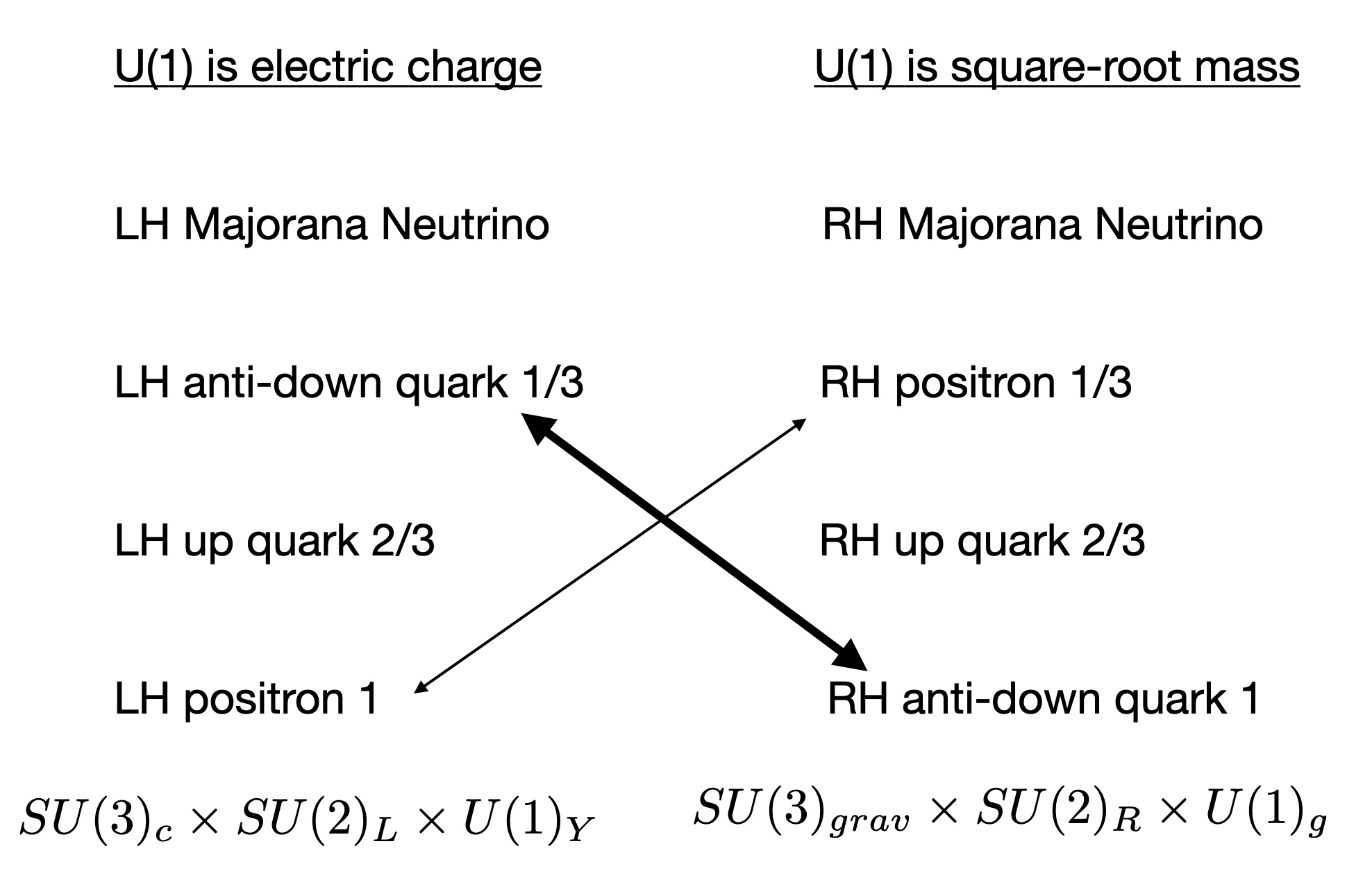
Figure 1: Left-Right fermions [9]

The $SU(3)_{grav}$ is to be interpreted as gravi-color and results in a gravitational interaction of the electron and up quark triplets. This interaction is confined to small length scales and is therefore not manifested in large scale gravity but we suggest that the effects of $SU(3)_{grav}$ will be important for understanding the gravitational effects of subatomic particles like the electron. We propose that the $SU(2)_{R}\otimes U(1)_{\gamma 2}$ will break into $U(1)_{grav}$ that corresponds to dark photon, whereas general relativity is emergent from the $SU(2)$ pre-gravitation. Theories have been proposed with the dark photon as a contender to explain dark matter[14] and testable experiments have also been proposed for the same[15]. We are also providing the emergence of the $U(1)_{grav}$ dark matter from $SU(2)_{R}\otimes U(1)_{\gamma 2}$ symmetry breaking where $SU(2)_{R}$ is giving us the ”Lorentz bosons” as mediators for chiral gravity. $SU(2)$ chiral gravity has been used in Loop quantum gravity as the gauge group for Ashtekar variables [16] that are cannonical variables in spatial hypersrufaces in the ADM formalism of gravity [17].

The understanding of gravity is very intrinsically related to the problem of mass. Why the stress-energy tensore bends spacetime? The problem of mass is also related to the problem of three generations, why the three generations are exactly similar apart from their mass? In the next section we try to answer this and our internal space (not internal in a pre-spacetime octonionic space) of SU(3) generation.

IV Triality, Jordan matrices, Spin(9), and three generations

In the above analysis, we have invoked an $SU(3)$ for three generations. The existence of three generations can be motivated from the triality of $SO(8)$, its relation to the octonions, and their associated exceptional Lie groups. Triality is also crucial in explaining the observed mass ratios for the three generations [9].

There have been some recent attempts to understand the three generations of fermions through the language of octonions. Gillard and Gresnigt talk about the three generations of fermions through the algebra of Sedenions and $\mathbb{C}l(8)$ [18]. The broader purview of the community is shifting towards the view that the triality of SO(8) is related to the three generations. We have oursleves related the three generations using the 3x3 Hermitian Jordan matrices with octonionic entries [2, 9] and obeying the exceptional Jordan algebra whose automorphism group is $F_{4}$. The automorphism group of the complexified exceptional Jordan algebra is $E_{6}$; this group is also the symmetry group of the Dirac equation in 10D space-time. There have been attempts before to interpret one of the $SU(3)$ from the $SU(3)\otimes SU(3)\otimes SU(3)$ maximal subgroup of $E_{6}$ to represent the rotation group for 3 generations [19, 20].

We have $\mathbb{C}l(8)\cong\mathbb{C}l(9)^{0}$, therefore the three generations of fermions discussed in [18] are related to spinors that we will now create from $\mathbb{C}l(9)$. Another interesting thing to note is that $\mathbb{C}l(9)$ spinors will be 2x2 matrices with octonionic entries, therefore we will show shortly how our previous work on three generations from $J_{3}(\mathbb{O})$ and Gresnigt’s construction [18] are related to three generations via triality.

Consider the following matrices:

$$ie_{i}\sigma_{x},\quad\sigma_{y},\quad\sigma_{z}$$

Here $e_{i}$ are the octonions, and $\sigma_{i}$ are the Pauli matrices, therefore the algebra is $\mathbb{H}\otimes\mathbb{O}$. These 9 matrices square to -1, and anti-commute with each other, therefore these can be used to make the generators of $\mathbb{C}l(9)$. Let’s call the generators as $\gamma_{i}$, i = 1,.., 9.

The fermionic creation and annihilation operators satisfying

$$\{\alpha_{i},\alpha_{j}\}=0\quad\forall\quad i,j\quad\text{form the MTIS}$$ (12)

and are given as:

$$\alpha_{1}=(\gamma_{1}+i\gamma_{9})/2=\begin{bmatrix}i&ie_{1}\\ ie_{1}&-i\\ \end{bmatrix}$$ (13)

$$\alpha_{2}=(\gamma_{2}+i\gamma_{8})/2=\begin{bmatrix}0&ie_{2}-1\\ ie_{2}+1&0\\ \end{bmatrix}$$ (14)

$$\alpha_{3}=(\gamma_{3}+i\gamma_{7})/2=\begin{bmatrix}0&ie_{3}-e_{7}\\ ie_{3}-e_{7}&0\\ \end{bmatrix}$$ (15)

$$\alpha_{4}=(\gamma_{4}+i\gamma_{6})/2=\begin{bmatrix}0&ie_{4}-e_{6}\\ ie_{4}-e_{6}&0\\ \end{bmatrix}$$

These are the annihilation operators and correspondingly we will have the creation operators $\alpha^{\dagger}_{i}$s. The idempotent V is given as:

$$V=\alpha_{1}\alpha_{2}\alpha_{3}\alpha_{4}\alpha_{4}^{\dagger}\alpha_{3}^{\dagger}\alpha_{2}^{\dagger}\alpha_{1}^{\dagger}$$ (17)

The total 16 spinors created (following Furey and Dixon [21, 22, 23, 24]) by acting the creation operator on the idempotent are given by:

$$V$$ (18)

$$\alpha_{1}^{\dagger}V,\hskip 3.41432pt\alpha_{2}^{\dagger}V,\hskip 3.41432pt\alpha_{3}^{\dagger}V,\hskip 3.41432pt\alpha_{4}^{\dagger}V$$ (19)

$$\alpha_{2}^{\dagger}\alpha_{1}^{\dagger}V,\hskip 3.41432pt\alpha_{3}^{\dagger}\alpha_{2}^{\dagger}V,\hskip 3.41432pt\alpha_{4}^{\dagger}\alpha_{3}^{\dagger}V,\hskip 3.41432pt\alpha_{1}^{\dagger}\alpha_{4}^{\dagger}V,\hskip 3.41432pt\alpha_{4}^{\dagger}\alpha_{3}^{\dagger}V,\hskip 3.41432pt\alpha_{4}^{\dagger}V\alpha_{2}^{\dagger}V$$ (20)

$$\alpha_{3}^{\dagger}\alpha_{2}^{\dagger}\alpha_{1}^{\dagger}V,\hskip 3.41432pt\alpha_{4}^{\dagger}\alpha_{3}^{\dagger}\alpha_{2}^{\dagger}V,\hskip 3.41432pt\alpha_{1}^{\dagger}\alpha_{4}^{\dagger}\alpha_{3}^{\dagger}V,\hskip 3.41432pt\alpha_{1}^{\dagger}V\alpha_{1}^{\dagger}V\alpha_{1}^{\dagger}V$$ (21)

$$\alpha_{4}^{\dagger}\alpha_{3}^{\dagger}\alpha_{2}^{\dagger}\alpha_{1}^{\dagger}V$$ (22)

It is interesting to note that the spinors created this way are 2x2 matrices with octonionic entries. The 2x2 exceptional Jordan matrices are spinors of spin(10). It has been shown by Dray and Manogue [25] that $SU(2,\mathbb{O})\cong spin(9)$, $Sl(2,\mathbb{O})\cong spin(1,9)$. Therefore, the 16 spinors form the subalgebra of $J_{2}(\mathbb{O})$. Also, the 16 spinors from $\mathbb{C}l(9)$ obtained here are related to the 16 spinors created by Gresnigt from $Cl(8)$ to understand three generations via $Cl(9)^{0}$.This relates the three generations created by Gresnigt to our work in $J_{3}(\mathbb{O})$ via triality in the following manner:

Triality of octonions is a map from $\mathbb{O}\otimes\mathbb{O}\otimes\mathbb{O}\rightarrow\mathbb{R}$ that is achieved via the group SO(8) [26]. The octonionic spinors of $\mathbb{C}l(6)$ that are to be interpreted as particles under $SU(3)_{c}\otimes U(1)_{em}$ [21, 24, 23] can be mapped to an element of $J_{2}(\mathbb{O})$ via the following map:

$$\mathbb{O}\rightarrow\begin{pmatrix}charge(\mathbb{O})&\mathbb{O}\\ \mathbb{O}^{*}&charge(\mathbb{O})\\ \end{pmatrix}$$ (23)

Here $charge(\mathbb{O})$ depicts the $U(1)_{em}$ charge corresponding to that octonion. And three elements of $J_{2}(\mathbb{O})$ with same diagonal entries a, b, c and octonionic entries x, y, z respectively can be mapped to an element of $J_{3}(\mathbb{O})$ as follows

$$J_{2}(\mathbb{O})\otimes J_{2}(\mathbb{O})\otimes J_{2}(\mathbb{O})\rightarrow\begin{pmatrix}(b+c)/2&y^{*}&z\\ y&(a+b)/2&x^{*}\\ z^{*}&x&(c+a)/2\\ \end{pmatrix}$$ (24)

We can now calculate the eigen-values of these matrices to obtain real numbers [27]. It has been shown in [9] that the eigen-values are related to the mass-ratios of charged fermions. Therefore while going from $\mathbb{O}\otimes\mathbb{O}\otimes\mathbb{O}$ all the way to $J_{3}(\mathbb{O})$ and then to its eigen-values, we are invoking the triality that is related to the three generations. The problem of the three generations is also the problem of the mass ratios!

$G_{2}$ is the automorphism group of the Octonions and has the maximal subgroup $SU(3)$ responsible for the colour of particles written in octonionic representation. $F_{4}$ is the automorphism group of $J_{3}(\mathbb{O})$ and has the maximal subgroup $SU(3)\otimes SU(3)$ where the other $SU(3)$ comes for generation [19]. All the three generations follow same spinorial dynamics, the only difference is between the mass, and it is a standard procedure in QFTs to write the three generations field $\psi$ as a $3\times 1$ column vector under $U(3)$. Post symmetry breaking of $SU(2)\otimes U(1)$, the three generations obtain different mass and hence different Yukawa potentials, they can no longer be written as 3$\otimes$1 column vector and the $U(3)$ group breaks. However, the triality of the Octonions seems to suggest that there is some non-trivial relation between the three generations, therefore prior to Higgs mechanism, the group $SU(3)$ that comes from the maximal subgroup of $F_{4}$ is being used instead of $U(3)$.

V Discussion

V.1 The unaccounted for degrees of freedom

Our unified group $E_{8}\otimes E_{8}$ contains every fundamental structure including spacetime, all chiral fermions, and their three generations, and all bosons. However this comes with some additional degrees of freedom whose states cannot be identified with our usual standard model particles. In this section, we attempt to give certain explanations for these unaccounted degrees of freedom. Each E₈ will give us ten unaccounted states, with five being conjugate (anti-particle) to the other five. We list the five independent unaccounted states from Eqn. (11):

$$(1,3,3,1)(2)\qquad(3,\bar{3},3.1)(0)\qquad(\bar{3},\bar{3},1,1)(2)$$

$$(\bar{3},1,3,2)(1)\qquad(3,1,\bar{3},1)(2)$$

Post symmetry breaking the electric charges corresponding to the above states in that order are 2/3, 0, 2, (2/3 and 1/3 doublet), and 2/3 respectively.

We are not very sure of these 72 fermionic particles and their anti-particles but as in $SU(5)$ or $SO(10)$ GUTs, these particles might be consumed during the process of symmetry breaking like Goldstone bosons. In SU(5) GUT as mentioned in [28], we face a situation where we get 24 gauge bosons out of which just 12 are standard model gauge bosons while the rest have not been confirmed experimentally . We could give similar analogy that out of these many degrees of freedom there may be some Goldstone boson type particles which would be eaten by some gauge fields. These Goldstone bosons are results of I SSB, $E_{8}\otimes E_{8}$ to our gauge group. II SSB will occur as $SU(2)\otimes U(1)\rightarrow U(1)$ and there released bosons gets eaten by Weak bosons for left chiral part and Weak-Lorentz bosons for right side. There are a total of 144 unaccounted fermions from each $E_{8}$, the total from both sides is 288. The total number of physical fermions from our theory are also 144, so there is a 1:2 ratio of accounted and unaccounted fermions. Working with a large group such as $E_{8}\otimes E_{8}$, it is challenging to account for all degrees of freedom but the main result of this paper that motivated the authors to pursue this project is that we can account for three generations of fermions, all the gauge bosons that include the ones for pre-gravitation, and spacetime from the representation of $E_{8}\otimes E_{8}$. This is in agreement with our proposed left-right symmetric theory on a pre-spacetime manifold where the bosons and fermions are on an equal footing. In order to account for these unaccounted fermions, further work needs to be done after modifying the Lagrangian written in [2].

V.2 Overview of the octonionic theory

Our theory is a matrix-valued Lagrangian dynamics on an octonionic space, motivated as a pre-quantum, pre-spacetime theory, i.e. a reformulation of quantum field theory which does not depend on an external classical time [29]. It is a generalisation of Adler’s theory of trace dynamics, so as to include pre-gravitation. Quantum field theory and classical space-time and gravitation are emergent from this dynamics under suitable approximations. The fundamental universe is a collection of ‘atoms of space-time-matter’, an atom being a 2-brane described by matrix-valued dynamical variables on octonionic space and having the action principle (of the unified interactions)

$$\frac{S}{\hbar}=\int d\tau\;{\cal L}\qquad;\qquad\mathcal{L}=\frac{1}{2}Tr\biggl{[}\biggr{.}\dfrac{L_{p}^{2}}{L^{2}}\dot{\widetilde{Q}}_{1}^{\dagger}\;\dot{\widetilde{Q}}_{2}\biggr{]}$$ (25)

This action defines a 2-brane residing on a split-bioctonionic space. This means that each of the two matrices ${\widetilde{Q}_{1}}$ and ${\widetilde{Q}_{2}}$ have sixteen components, one component per coordinate direction of the split bioctonion. This 16-dim space has $E_{8}\otimes E_{8}$ symmetry. We separate the two dynamical variables into bosonic and fermionic parts, each of which again has sixteen coordinate components:

$$\dot{\widetilde{Q}}_{1}^{\dagger}=\dot{\widetilde{Q}}_{B}^{\dagger}+\dfrac{L_{p}^{2}}{L^{2}}\beta_{1}\dot{\widetilde{Q}}_{F}^{\dagger};\ \qquad\dot{\widetilde{Q}}_{2}=\dot{\widetilde{Q}}_{B}+\dfrac{L_{p}^{2}}{L^{2}}\beta_{2}\dot{\widetilde{Q}}_{F}$$ (26)

Left-Right symmetry breaking separates the bosonic dynamical variable into its left-chiral part $q_{B}$ defined over 8D octonionic space and the right chiral part $\dot{q}_{B}$ defined over the 8D splt octonionic space. Similarly the fermionic dynamical variable separates into its left chiral part $q_{F}$ defined over 8D octonionic space and its right chiral part $\dot{q}_{F}$ defined over the split octonionic space.

$${\dot{\widetilde{Q}}_{B}}=\frac{1}{L}(i\alpha q_{B}+L\dot{q}_{B});\qquad{\dot{\widetilde{Q}}_{F}}=\frac{1}{L}(i\alpha q_{F}+L\dot{q}_{F})$$ (27)

The Yang-Mills coupling constant $\alpha$ arises as a consequence of the symmetry breaking, prior to which the theory is scale invariant, having only an associated length scale $L$ but no other free parameter. The symmetries of the bioctonionic space are spacetime symmetries with the full symmetry being $E_{8}\otimes E_{8}$ and with symmetry breaking introducing branching as discussed earlier in the paper, and also introducing interactions and coupling constants.

By defining new variables

$$q^{\dagger}_{1}=q_{B}^{\dagger}+\frac{L_{P}^{2}}{L^{2}}\beta_{1}q^{\dagger}_{F}\qquad;\qquad q_{2}=q_{B}+\frac{L_{P}^{2}}{L^{2}}\beta_{2}q_{F}$$ (28)

we can also express the Lagrangian as

$${\cal L} =\frac{L_{P}^{2}}{2L^{2}}\;Tr\left[\left(\dot{q}_{1}^{\dagger}+\frac{i\alpha}{L}q_{1}^{\dagger}\right)\times\left(\dot{q}_{2}+\frac{i\alpha}{L}q_{2}\right)\right]$$ (29)

$$=\frac{L_{P}^{2}}{2L^{2}}\;Tr\left[\dot{q}_{1}^{\dagger}\dot{q}_{2}-\frac{\alpha^{2}}{L^{2}}q_{1}^{\dagger}q_{2}+\frac{i\alpha}{L}q_{1}^{\dagger}\dot{q}_{2}+\frac{i\alpha}{L}\dot{q}_{1}^{\dagger}q_{2}\right]$$

We can next expand each of these four terms inside of the trace Lagrangian as explored thoroughly in the paper [30], using the definitions of $q_{1}$ and $q_{2}$ given above:

$$\dot{q}_{1}^{\dagger}\dot{q}_{2} =\dot{q}_{B}^{\dagger}\dot{q}_{B}+\frac{L_{P}^{2}}{L^{2}}\dot{q}_{B}^{\dagger}\beta_{2}\dot{q}_{F}+\frac{L_{P}^{2}}{L^{2}}\beta_{1}\dot{q}_{F}^{\dagger}\dot{q}_{B}+\frac{L_{P}^{4}}{L^{4}}\beta_{1}\dot{q}_{F}^{\dagger}\beta_{2}\dot{q}_{F}$$ (30)

$$q_{1}^{\dagger}q_{2} =q_{B}^{\dagger}{q}_{B}+\frac{L_{P}^{2}}{L^{2}}q_{B}^{\dagger}\beta_{2}{q}_{F}+\frac{L_{P}^{2}}{L^{2}}\beta_{1}q_{F}^{\dagger}{q}_{B}+\frac{L_{P}^{4}}{L^{4}}\beta_{1}q_{F}^{\dagger}\beta_{2}{q}_{F}$$

$$q_{1}^{\dagger}\dot{q}_{2} =q_{B}^{\dagger}\dot{q}_{B}+\frac{L_{P}^{2}}{L^{2}}q_{B}^{\dagger}\beta_{2}\dot{q}_{F}+\frac{L_{P}^{2}}{L^{2}}\beta_{1}q_{F}^{\dagger}\dot{q}_{B}+\frac{L_{P}^{4}}{L^{4}}\beta_{1}q_{F}^{\dagger}\beta_{2}\dot{q}_{F}$$

$$\dot{q}_{1}^{\dagger}q_{2} =\dot{q}_{B}^{\dagger}{q}_{B}+\frac{L_{P}^{2}}{L^{2}}\dot{q}_{B}^{\dagger}\beta_{2}{q}_{F}+\frac{L_{P}^{2}}{L^{2}}\beta_{1}\dot{q}_{F}^{\dagger}{q}_{B}+\frac{L_{P}^{4}}{L^{4}}\beta_{1}\dot{q}_{F}^{\dagger}\beta_{2}{q}_{F}$$

This form of the Lagrangian displays terms for the bosonic variables (gauge fields), the fermionic part of the action (leading to the Dirac equations upon variation), and terms bilinear in fermionic varaibles (related to the Higgs). A preliminary analysis of this Lagrangian, relating it to three generations, has been carried out in [2]. In future work we hope to report as to how the Lagrangian relates to the fermions and bosons reported in the present paper, including the unaccounted for terms discussed in the previous subsection. We note that the (8x3=24) fermions of the three generations contribute 24 x 24 = 576 = 288 x 2 terms to the Lagrangian, which are bilinear in $q_{F}$ and $\dot{q}_{F}$. It is striking that this is twice the number 288 of unaccounted degrees of freedom. Recall also that there are 144 physical fermions as demonstrated earlier in the paper.The terms bilinear in the $q_{F}$ and $\dot{q}_{F}$ possibly describe the two Higgs doublets of the theory, and hence it could be that the 288 unaccounted d.o.f. go into constituting two composite Higgs (144 for each Higgs) and hence that there are no new predicted fermions. Such a possibility is currently under investigation. We also note that there are (208-144=64=32x2) non-fermionic d.o.f. and these account for the 32 bosons corresponding to the (2x16=32) space-time d.o.f. (8+8 = 16 dimensional split bioctonioc space and the factor 2 because this space is complexified).

Such a pre-spacetime, pre-quantum dynamics is in principle essential at all energy scales, not just at the Planck energy scale [2]. Whenever a physical system has only quantum sources, the coordinate geometry of spacetime is non-commutative; and when that is an octonionic geometry, the spacetime symmetries result in the standard model and its unification with pre-gravitation, as we have seen in the present paper. Fermionic states are spinors (left minimal ideals) of the Clifford algebra $Cl(6)$ made from octonionic chains. Following the earlier work of other researchers, we constructed such $Cl(6)$ states for three generations of left chiral and right chiral quarks and leptons [9, 10], and their associated bosons. We argued in these papers that pre-gravitation is the right-handed counterpart of the standard model with the associated symmetry group being $E_{6}\otimes E_{6}$. This is confirmed by the reps found in the present paper; furthermore the $E_{8}\otimes E_{8}$ symmetry unifies the spacetime with the matter and gauge degrees of freedom living on this spacetime, into a common unified description. Doing so has also introduced new so-called unaccounted fermions which are truly beyond the standard model, and whose physical significance and experimental consequences remain to be understood.

The Dirac equation resulting from this Lagrangian dynamics has an $E_{6}$ symmetry, and its real eigenvalues are determined by the characteristic equation of the exceptional Jordan algebra $J_{3}(8)$, whose automorphism group is $F_{4}$. These eigenvalues can be found for three generations of Dirac quarks and Dirac leptons, and also for three generations of left chiral fermions or right chiral fermions. Since the left chiral fermions are charge eigenstates, and right chiral fermions are square-root mass eigenstates, these eigenvalues help explain the strange mass ratios of quarks and leptons [9]. This is because experimental measurements invariably employ charge eigenstates, which are distinct from mass eigenstates.

The octonionic theory has similarities with string theory, but also differs from it in crucial ways. Our theory is also for extended objects in 10D spacetime and has an $E_{8}\otimes E_{8}$ symmetry. However, we build the Fock space of states for particles, not on a 10D Minkowski spacetime vacuum, but on the octonion-valued twistor space, which is a spinor spacetime, as if a ‘square-root’ of the 10D Minkowski spacetime. The non-commutative octonion geometry has to be an essential feature of quantum theory even at low energy scales, not just at the Planck scale. Only then can the standard model be understood. The extra dimensions are complex and not to be compactified - these are the dimensions along which the internal symmetries lie. Finally, the Hamiltonian of the theory is in general not self-adjoint; thus enabling the quantum-to-classical transition, and otherwise becoming self-adjoint in the approximation in which quantum field theory is recovered from trace dynamics. Further evidence for trace dynamics comes from the result that the theory admits supra-quantum nonlocal correlations predicted by the Popescu-Rohrlich bound in the CHSH inequality, but disallowed by quantum mechanics. This constitutes strong evidence that quantum theory is approximate, and emergent from trace dynamics in a coarse-grained approximation. [31]

The octonionic theory employs the octonions to define a non-commutative coordinate geometry. The symmetries of the geometry dictate the existence of standard model chiral fermions, gauge bosons, and pre-gravitation. Clifford algebras made from octonionic chains define spinorial states for the fermions, and the exceptional Jordan algebra determines values of the standard model parameters. The matrix-valued Lagrangian dynamics determines evolution of these particles. Classical general relativity emerges from pre-gravitation as a result of a quantum-to-classical spontaneous localisation which confines classical systems to our familiar 4D spacetime. However, quantum systems always live in the octonionic space, which has complex extra dimensions which are never compactified. Further work is in progress so as to attempt taking this unification program to completion.

References

- Tejinder P. Singh [2020] Tejinder P. Singh, Trace dynamics and division algebras: towards quantum gravity and unification. (Zeitschrift fur Naturforschung A 76, 131, DOI: https://doi.org/10.1515/zna– 2020–0255, arXiv:2009.05574v44 [hep–th], 2020).
- Tejinder P. Singh [2022] Tejinder P. Singh, Quantum gravity effects in the infra-red: a theoretical derivation of the low energy fine structure constant and mass ratios of elementary particles (Eur. Phys. J. Plus 137, 664 (2022). https://doi.org/10.1140/epjp/s13360-022-02868-4, arXiv:2205.06614, 2022).
- Abhinash Kumar Roy and Anmol Sahu and Tejinder P. Singh [2020] Abhinash Kumar Roy and Anmol Sahu and Tejinder P. Singh, Trace dynamics, and a ground state in spontaneous quantum gravity; 10.1142/s021773232150019x (Modern Physics Letters A, 2020).
- Gross, David J. and Harvey, Jeffrey A. and Martinec, Emil and Rohm, Ryan [1985] Gross, David J. and Harvey, Jeffrey A. and Martinec, Emil and Rohm, Ryan, Heterotic String (Phys. Rev. Lett. 54, 502; 10.1103/PhysRevLett.54.502, 1985).
- Volker Braun and Yang-Hui He and Burt A Ovrut and Tony Pantev [2005] Volker Braun and Yang-Hui He and Burt A Ovrut and Tony Pantev, A Standard Model from Heterotic String theory (Journal of High Energy Physics; 10.1088/1126-6708/2005/06/039, 2005).
- Corinne A. Manogue, Tevian Dray, Robert A. Wilson [2022] Corinne A. Manogue, Tevian Dray, Robert A. Wilson, Octions: An E8 description of the Standard Model (https://doi.org/10.48550/arXiv.2204.05310, arXiv:2204.05310, 2022).
- Matej Pavsic [2008] Matej Pavsic, A novel view on the physical origin of E8 (J. Phys. A: Math. Theor. 41 332001, arXiv:0806.4365, 2008).
- Slansky, R. [1981] Slansky, R., Group Theory for Unified Model Building (Phys. Rept. 79, 1, 1981).
- V. Bhatt, R. Mondal, V. Vaibhav, T.P. Singh [2022] V. Bhatt, R. Mondal, V. Vaibhav, T.P. Singh, Majorana neutrinos, exceptional Jordan algebra, and mass ratios for charged fermions (J. Phys. G: Nucl. Part. Phys. 49 045007, arXiv:2108.05787, 2022).
- Vatsalya Vaibhav, Tejinder P Singh [2021] Vatsalya Vaibhav, Tejinder P Singh, Left-right symmetric fermions and sterile neutrinos from complex split biquaternions and bioctonions (arXiv preprint arXiv:2108.01858, 2021).
- Furey [2018a] C. Furey, A demonstration that electroweak theory can violate parity automatically (leptonic case) (International Journal of Modern Physics A, Volume 33, Issue 04, Pg 1830005, 2018).
- Penrose R. [1967] Penrose R., Twistor Algebra (Journal of Mathematical Physics. 8 (2): 345–366. Bibcode:1967JMP…..8..345P. doi:10.1063/1.1705200, 1967).
- Hitchin [2018] N. Hitchin, SL(2) over the octonions (Mathematical Proceedings of the Royal Irish Academy) (https://arxiv.org/abs/1805.02224, 10.48550/ARXIV.1805.02224, 2018).
- Essig, R. et al [2013] Essig, R. et al, Dark Sectors and New, Light, Weakly-Coupled Particles (arXiv:1311.0029 https://doi.org/10.48550/arXiv.1311.0029, 2013).
- Holdom, Bob [1986] Holdom, Bob, Two U(1)’s and charge shifts (Physics Letters B. 166 (2): 196–198. Bibcode:1986PhLB..166..196H. doi:10.1016/0370-2693(86)91377-8. ISSN 0370-2693, 1986).
- Ashtekar, A [1986] Ashtekar, A, New variables for classical and quantum gravity (Physical Review Letters. 57 (18): 2244–2247. Bibcode:1986PhRvL..57.2244A. doi:10.1103/physrevlett.57.2244. PMID 10033673., 1986).
- Arnowitt, R.; Deser, S.; Misner, C. [1959] Arnowitt, R.; Deser, S.; Misner, C., Dynamical Structure and Definition of Energy in General Relativity (Physical Review. 116 (5): 1322–1330. Bibcode:1959PhRv..116.1322A. doi:10.1103/PhysRev.116.1322, 1959).
- Adam B Gillard, Niels G Gresnigt [2019] Adam B Gillard, Niels G Gresnigt, Three fermion generations with two unbroken gauge symmetries from the complex sedenions (Eur. Phys. J. C 79, 446 (2019). https://doi.org/10.1140/epjc/s10052-019-6967-1, arXiv:1904.03186, 2019).
- Latham Boyle [2020] Latham Boyle, The Standard model, the Exceptional Jordan algebra, and Triality (e-print, arXiv:2006.16265v1 [hep–th] (2020)., 2020).
- Ivan Todorov, Michel Dubois-Violette [2017] Ivan Todorov, Michel Dubois-Violette, Deducing the symmetry of the Standard Model from the automorphism and structure groups of the exceptional Jordan algebra (https://doi.org/10.48550/arXiv.1806.09450, 2017).
- C. Furey [2015] C. Furey, Standard Model Physics from an Algebra? (Ph. D. thesis, University of Waterloo. arXiv:1611.09182 [hep-th], 2015., 2015).
- Geoffrey M. Dixon [1994] Geoffrey M. Dixon, . Division algebras, octonions, quaternions, complex numbers and the algebraic design of physics (Kluwer, Dordrecht, 1994., 1994).
- Furey [2018b] C. Furey, as a symmetry of division algebraic ladder operators (The European Physical Journal C, 10.1140/epjc/s10052-018-5844-7, 2018).
- Furey [2018c] C. Furey, Three generations, two unbroken gauge symmetries, and one eight-dimensional algebra; 10.1016/j.physletb.2018.08.032 (Physics Letters B, 2018).
- Tevian Dray, Corinne A. Manogue [2010] Tevian Dray, Corinne A. Manogue, Octonionic Cayley Spinors and E6 (Comment. Math. Univ. Carolin. 51, 193-207, arXiv:0911.2255, 2010).
- C.Baez [2001] J. C.Baez, The Octonions (Bull.Am.Math.Soc.39:145-205,2002, arXiv:math/0105155 [math.RA], 2001).
- Tevian Dray, Corinne A. Manogue [1999] Tevian Dray, Corinne A. Manogue, The Exceptional Jordan Eigenvalue Problem (IJTP 38, 2901-2916, arXiv:math-ph/9910004, 1999).
- Cheng and Li [1984] T. P. Cheng and L. F. Li, Gauge theory of elementary particle physics (Oxford University Press, Oxford, UK, 1984).
- Singh, Tejinder P. [2021] Singh, Tejinder P., Quantum theory without classical time: a route to quantum gravity and unification (arXiv:2110.02062v1, 2021).
- Raj and Singh [2022] S. Raj and T. P. Singh, A Lagrangian with symmetry for the standard model and pre-gravitation I. – The bosonic Lagrangian, and a theoretical derivation of the weak mixing angle (arxiv.2208.09811 https://doi.org/10.48550/arxiv.2208.09811, 2022).
- Ahmed and Singh [2022] R. G. Ahmed and T. P. Singh, A violation of the Tsirelson bound in the pre-quantum theory of trace dynamics (arxiv.2208.02209 https://doi.org/10.48550/arxiv.2208.02209, 2022).