Stability of solitary waves in nonlinear Klein-Gordon equations

Abstract

The stability of topological solitary waves and pulses in one-dimensional nonlinear Klein-Gordon systems is revisited. The linearized equation describing small deviations around the static solution leads to a Sturm-Liouville problem, which is solved in a systematic way for the $-l\,(l+1)\,\mathop{\rm sech}^{2}(x)$-potential, showing the orthogonality and completeness relations fulfilled by the set of its solutions for all values $l\in\mathbb{N}$. This approach enables the linear stability of kinks and pulses of certain nonlinear Klein-Gordon equations to be determined. The inverse problem, which starts from Sturm-Liouville problem and obtains nonlinear Klein-Gordon potentials, is also revisited and solved in a direct way. The exact solutions (kinks and pulses) for these potentials are calculated, even when the nonlinear potential is not explicitly known. The kinks are found to be stable, whereas the pulses are unstable. The stability of the pulses is achieved by introducing certain spatial inhomogeneities.

1 Introduction

Nonlinear Klein-Gordon equations model a plethora of phenomena such as the existence of bound oscillatory states and resonance windows in the kink-antikink interaction [1, 2, 3, 4, 5] in the presence and in the absence of internal modes [6, 7, 8, 9], the fading of the kink’s wobbling due to the second-harmonic radiation [10, 11], the phase transitions in the Ginzburg-Landau theory [12, 13, 14], the motion of domain walls [15], and the existence of kinks with power-law tail asymptotics that give rise to long-range interactions in the even-higher-order field theories [16, 17].

In a one-dimensional system, the Hamiltonian corresponding to the nonlinear Klein-Gordon equation is a functional of the field $\varphi(x,t)$, defined in the following way:

$$H[\varphi(x,t)]=\int_{\mathbb{R}}\,dx\,\left\{\frac{\varphi_{t}^{2}(x,t)}{2}+\frac{\varphi_{x}^{2}(x,t)}{2}+U[\varphi(x,t)]\right\},$$ (1.1)

where $U[\varphi(x,t)]$ is the nonlinear Klein-Gordon potential, the integral is performed across the whole space $x\in\mathbb{R}$, and $t$ and $x$ subscripts henceforth denote the partial derivative with respect to time and position, respectively. Since the energy of the system must be finite, the spatial derivative of the field, $\varphi_{x}(x,t)$, should be a bounded function for all $x\in\mathbb{R}$ and $t\geq 0$.

From the Hamiltonian field equations [18], the one-dimensional nonlinear Klein-Gordon system is given by

$$\varphi_{tt}(x,t)-\varphi_{xx}(x,t)=-\frac{dU}{d\varphi}[\varphi(x,t)],$$ (1.2)

where the function $\varphi(x,t)\in C^{2}_{\infty}(\mathbb{R}\times[0,+\infty))$. Here, $C^{2}_{\infty}(\Omega)$ denotes the space of functions $f:\Omega\mapsto\mathbb{C}$ that are two times differentiable with continuous second order partial derivatives in $\Omega$, and such that $f$ and their first partial derivatives are bounded in $\Omega$. Throughout this study it is assumed that the nonlinear Klein-Gordon potential $U[\varphi(x,t)]$ has at least two extrema to guarantee the existence of kink or pulse-like solutions.

In particular, a pulse may emerge when the nonlinear potential $U[\varphi(x)]$ has a minimum and a maximum as two consecutive extrema, while the appearance of a topological wave called kink requires that $U[\varphi(x)]$ has two consecutive minima sharing the same value. Hereafter the function $\phi^{\rm st}_{p}(x)$ represents the static pulses and $\varphi^{\rm st}(x)$, the kinks at rest.

The dynamics and stability of the sech-shape solution of certain cubic potential were investigated in Ref. [19], where the pulse was found to be unstable. Moreover, kink solutions $\varphi^{\rm st}(x)$ have been derived for the sine-Gordon potential [20], the double sine-Gordon potential [21], and the $\varphi^{n}$ ($n=4,6,8$) potentials [22, 23] (see also the recent reviews [24, 25, 9, 17] wherein developments of higher-order field theories are discussed). Since Eq. (1.2) is Lorentz invariant, traveling solutions can be obtained from the static solutions by a boost transformation.

At the boundaries, the topological waves verify

$$\lim_{x\to+\infty}\varphi(x,t) = \lim_{x\to-\infty}\varphi(x,t)\pm Q,$$ (1.3)

where the signs $\pm$ refer to the kink and antikink solution, respectively, and the constant $Q>0$ is the so-called topological charge. The pulses also satisfy Eq. (1.3) setting $Q=0$.

As a matter of fact, the equations that govern physical systems, such as the propagation of magnetic flux along the Josephson junctions [26], the dynamics of the azimuthal angle of the unit vector of magnetization of ferromagnetic materials [27], the resonant soliton-impurity interactions [28], the unidirectional motion of kinks due to zero-average forces [29, 30, 31, 32], the stabilization of wobbling kinks [11], and the traveling of dislocations along the colloids [33], are modeled by nonlinear Klein-Gordon equations with external and parametric forces and damping. Therefore, the observation of these waves in nature and in experiments depends on their stability [34]. From the study of stability it can be determined whether the perturbed solution of Eq. (1.2) does not deviate too far from the exact solution when the perturbations are small enough, that is, whether the exact solution would be detected in a real system.

The stability of the sine-Gordon waves was studied by Scott more than 50 years ago, first by means of an average Lagrange method [20], and second by employing a more accurate technique, namely the eigenfunction expansion [35], introduced by Parmentier to study the stability of a nonlinear transmission line [36]. As a result of the second methodology, a Sturm-Liouville problem was obtained and discussed, although not completely solved. Its spectrum has both a discrete and a continuous part [37]. Indeed, since Eq. (1.2) is translationally invariant, there is always a zero mode associated to the zero eigenvalue (zero frequency) and to an eigenfunction proportional to the spatial derivative of the field [38, 35]. The continuous spectrum exists due to the infinite domain [39].

The exact analytical solution of the Sturm-Liouville problem was found for the sine-Gordon kink, the $\varphi^{4}$ kink, the $\varphi^{6}$ kink, and also for the pulse of certain cubic potential [37, 22, 19, 23], among others. However, in some cases, only numerical solutions of this problem have been found either because the solution of Eq. (1.2) is implicit, as in the $\varphi^{8}$ equation [23], or because it has been impossible to analytically solve the corresponding Sturm-Liouville problem, as in the double sine-Gordon system [6].

The main goal of the current investigation is to revise the Sturm-Liouville problem equivalent to the one-dimensional Schrödinger equation with the Pöschl-Teller potential [40], $-l\,(l+1)\,\mathop{\rm sech}^{2}(x)$, $l\in\mathbb{N}$, which is associated to the stability of nonlinear waves of several aforementioned nonlinear Klein-Gordon potentials. This potential is one of the most useful potentials in mathematical physics. It appears in Optics [41], in Quantum Mechanics [42] (see also page 768 in Ref. [43], page 94 in Ref. [44], and page 73 in Ref. [45]), in the $N$-soliton solution of the Korteweg and de-Vries equation [46], and in the stability study of certain static solutions [47]. The above potential, belongs to the special class of potentials for which the one-dimensional Schrödinger equation can be exactly solved in terms of special functions (see page 768 in Ref. [43]).

The inverse problem, proposed by Christ and Lee in Ref. [48] for the specific case of the kink solutions, investigates the existence of other nonlinear Klein-Gordon kinks or pulses whose stability is associated with the Pöschl-Teller potential? They started from the translational mode corresponding to the Pöschl-Teller potential, and partially, although not explicitly, constructed the sine-Gordon ($l=1$) and $\varphi^{4}$ ($l=2$) potentials. The explicit construction of the potential $U(\varphi)$ by solving the resulting differential equation for $U(\varphi)$ is due to Trullinger and Flesch [49]. They obtained two solutions for $U(\varphi)$, one for the odd values of $l$ and the other for the even values of $l$, and they found that these potentials can be expressed in terms of the Student’s $t$-distribution of probability theory.

Despite all these studies, to the best of our knowledge, there is no rigorous analysis of the corresponding Sturm-Liouville problem, nor a detailed proof of the orthogonality and completeness of its eigenfunctions for all values of $l\in\mathbb{N}$, nor a solution of the inverse problem in a direct way. It is the aim of the current study to complete the aforementioned studies.

Section 2 provides the outline of the linear stability analysis of the static solution, either $\varphi^{\rm st}(x)$ or $\phi^{\rm st}_{p}(x)$, of Eq. (1.2), and derives the associated Sturm-Liouville problem. This Section ends with a precise definition of the stability, which requires the positiveness of all the eigenvalues (squared eigenfrequencies). This definition is a consequence of the ansatz employed, in order to solve the Sturm-Liouville problem. The subsequent Section 3 solves the Sturm-Liouville problem with the potential, $-l\,(l+1)\,\mathop{\rm sech}^{2}(x)$, $l\in\mathbb{N}$, in a systematic way, including a detailed proof of the orthogonality and completeness relations. This is a very crucial result, since in practical applications the spatial component of the solution of certain perturbed nonlinear Klein-Gordon equations is written as an expansion in the set of eigenfunctions (see e.g. §5.2 on page 144 in Ref. [24]). Specifying the values of $l=1$ and $l=2$, it is shown that the sine-Gordon and $\varphi^{4}$ kinks, respectively, are stable. The values of $l=3$ and $l=2$ are related with the unstable pulses of the cubic and quartic potentials, respectively.

Section 4 addresses this issue and reconstructs the theory in a similar way to that in Ref. [49]; however, the problem is solved in a more direct way, without using the Student’s $t$-distribution. Our procedure has two advantages with respect to the previous analyses of Refs. [48, 49]. First, our analysis is valid for all values of $l$ and the solution of the second-order differential equation for $U(\varphi)$ is represented in a closed form in terms of the hypergeometric function, where $l$ is a parameter. Second, all kink solutions can be obtained by a recurrence relation, where the sequence of kinks depends on the value of $l$. Section 4 obtains two families of nonlinear Klein-Gordon potentials such that the Pöschl-Teller potential appears in their corresponding Sturm-Liouville problems. For the first family, the exact analytical kinks are obtained. It is demonstrated that all kinks are stable. For the second family, the pulses are derived. Although all the pulses found are unstable, Section 5 provides guidelines for their stabilization through inhomogeneous forces. Finally, Section 6 discusses our main results and draws general conclusions.

2 The nonlinear Klein-Gordon equation and its corresponding Sturm-Liouville problem

Due to the Lorentz invariance of Eq. (1.2), it is sufficient to investigate the stability of the static kink [24], $\varphi(x,t)=\varphi^{\rm st}(x)$, which satisfies the following equation

$$\varphi^{\rm st}_{xx}(x)=\frac{dU}{d\varphi}[\varphi^{\rm st}(x)],$$ (2.1)

where the nonlinear Klein-Gordon potential $U$ has at least two local minima, which are reached by $U[\varphi^{\rm st}(x)]$ as $x\to\pm\infty$. Notice that, Eq. (2.1) resembles the second Newton law for a particle in a potential $-U[\varphi^{\rm st}(x)]$ [48]. This is the reason why $-U$ is called a pseudo-potential [50]. Within this framework, the variables $x$ and $\varphi^{\rm st}(x)$ play the role of time and position, respectively.

By integrating Eq. (2.1), the first integral of motion reads

$$E=\frac{(\varphi^{\rm st}_{x})^{2}}{2}-U[\varphi^{\rm st}(x)],$$ (2.2)

where $E$ denotes the total energy of the Newtonian particle, and $(\varphi^{\rm st}_{x})^{2}/2$ its kinetic energy. Three different cases are distinguished according to the value of $E$. When the energy $E>M$, where $M$ is the maximum of the pseudo-potential, the particle is always moving, similar to the rotatory motion of the simple pendulum, see Fig. 1. If $m\leq E<M$, where $m$ is the minimum of the pseudo-potential, the particle oscillates except for $E=m$ when the particle remains at rest. The separatrix at $E=M$ separates oscillatory and rotatory motions, see the phase portrait in Fig. 1. The kink (antikink), $\varphi^{\rm st}(x)$, is represented precisely by the separatrix of the dynamical system (2.1), which connects two maxima of the pseudo-potential $-U[\varphi^{\rm st}(x)]$, that is, two minima of the potential $U[\varphi^{\rm st}(x)]$, when $x\to\pm\infty$. As a consequence,

$$\lim_{x\to\pm\infty}\frac{dU}{d\varphi}[\varphi^{\rm st}(x)]=0,$$ (2.3)

$$\lim_{x\to\pm\infty}\frac{d^{2}U}{d\varphi^{2}}[\varphi^{\rm st}(x)]\geq 0.$$ (2.4)

Without any loss of generality, it is assumed that the minimum of the potential is reached at zero, that is,

$$\lim_{x\to\pm\infty}U[\varphi^{\rm st}(x)]=0.$$ (2.5)

This implies that $U[\varphi^{\rm st}(x)]\geq 0$ between the two minima. Furthermore, it sets $E=0$ in (2.2). Notice that these conditions on the potential and its derivatives are also satisfied by a static pulse, solution of Eq. (2.1). Indeed, a pulse lies on the separatrix that begins and ends at the same equilibrium point, which is a minimum of the potential.

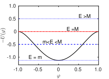
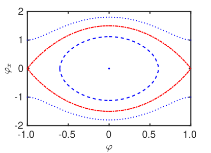
Figure 1: Left-hand panel: the pseudo-potential $-U(\varphi)$ is shown (solid black line), and four values of energy related with different types of motions (see the text): $E=m$ and $E>M$ (dotted blue lines), $m<E<M$ (dashed blue line), and $E=M$ (dot-dashed red line). Right-hand panel: the separatrix, represented with a dot-dashed red line ($E=M$), it separates the region where the motion is unbounded (dotted blue line, $E>M$) from the region where the oscillatory motion takes place (dashed blue line, $m<E<M$). The particle is at rest at the origin.

From Eq. (2.2), it follows that the static kink, or static pulse, can be calculated by performing the following integral

$$\int\frac{d\varphi}{\sqrt{2\,U(\varphi)}}=x+C,$$ (2.6)

where the constant $C$ is set to zero due to the translational invariance. By considering the sine-Gordon potential

$$U(\varphi)=1-\cos(\varphi)$$ (2.7)

in Eq. (2.6), and by integration, the static kink has the form

$$\varphi^{\rm st}(x)=4\,\arctan[\exp(x)].$$ (2.8)

By applying a similar procedure with the $\varphi^{4}$ potential

$$U(\varphi)=\frac{(1-\varphi^{2})^{2}}{2},$$ (2.9)

we obtain the static kink

$$\varphi^{\rm st}(x)=\tanh(x).$$ (2.10)

By integrating Eq. (2.6) with the cubic and quartic potentials shown in the first column of Table 1, the static pulses are calculated (second column of Table 1). The second-order differential equation (2.1) with the cubic and quartic potentials also appears when we find soliton solutions in the KdV equation [51, 46] and in the nonlinear Schrödinger (NLS) equation [52, 34, 53], respectively. The KdV soliton is non-topological and has the same shape as the pulse of the cubic potential, whereas the envelope part of the NLS soliton and the pulse of the quartic potential have the same shape.

$U(\phi)$	$\phi^{\rm st}_{p}(x)$	$\psi^{\rm st}(x)$	$V(x)$	$\omega_{ph}$
$2\,\phi^{2}\,(1-\phi)$	$\frac{1}{\,\cosh^{2}(x)}$	$\frac{-2\,\tanh(x)}{\cosh^{2}(x)}$	$-\frac{12}{\cosh^{2}(x)}$	$2$
$\frac{\phi^{2}}{2}\,(1-\phi^{2})$	$\frac{1}{\,\cosh(x)}$	$\frac{-\tanh(x)}{\,\cosh(x)}$	$-\frac{6}{\cosh^{2}(x)}$	$1$

Table 1: For the cubic and quartic potentials, $U(\phi)$, the unstable solitary waves (pulses) $\phi^{\rm st}_{p}(x)$, the eigenfunction $\psi^{\rm st}(x)=d\phi^{\rm st}_{p}/dx$ associated to the zero frequency, the potential $V(x)$ (3.4), and the lowest frequency of the continuous spectrum, $\omega_{ph}$ are shown.

In order to discuss the stability of the static kink, $\varphi^{\rm st}(x)$, Eq. (1.2) is linearized around $\varphi^{\rm st}(x)$, that is, the function [36, 35]

$$\varphi(x,t)=\varphi^{\rm st}(x)+\Psi(x,t),$$ (2.11)

is introduced in Eq. (1.2). This implies that the function $\Psi(x,t)$ satisfies the following linear wave equation with a source term

$$\Psi_{tt}(x,t)-\Psi_{xx}(x,t)=-U^{\prime\prime}[\varphi^{\rm st}(x)]\Psi(x,t),$$ (2.12)

where the prime denotes the derivative of $U[\varphi(x)]$ with respect to $\varphi(x)$. It is important to bear in mind that in the above relation (2.11), the second term should be small in comparison with $\varphi^{\rm st}(x)$. This can be achieved if the $L^{\infty}$-norm of $\Psi(x,t)$ is finite for all $t\geq t_{0}$, where $t_{0}$ is the initial time, that is, $\sup_{x\in\mathbb{R},t\geq t_{0}}|\Psi(x,t)|<+\infty$, and sufficiently small in comparison with $\sup_{x\in\mathbb{R}}|\varphi^{\rm st}(x)|$. We recall that, since the energy of the system must be finite, $\varphi_{x}(x,t)$ should be a bounded function in $x\in\mathbb{R}$, then so should $\Psi_{x}(x,t)$.

The solution of Eq. (2.12) is represented by the following ansatz [36, 35, 17]

$$\Psi(x,t)=(c_{1}e^{i\omega t}+c_{2}e^{-i\omega t})\,\psi(x),$$ (2.13)

where $\psi(x)$ is a complex function and the complex constants $c_{1}$ and $c_{2}$ are chosen such that $\Psi(x,t)\in\mathbb{R}$. By inserting Eq. (2.13) into Eq. (2.12), it is straightforwardly deduced that $\psi(x)$ verifies the following Sturm-Liouville problem

$$\psi_{xx}(x)+\left(\omega^{2}-U^{\prime\prime}[\varphi^{\rm st}(x)]\right)\psi(x)=0,$$ (2.14)

where $\omega^{2}$ (squared eigenfrequencies) are the eigenvalues and it is required that $\psi(x)$ as well as its first derivative $\psi_{x}(x)$ are bounded and continuous functions on $\mathbb{R}$ (recall that the energy of the system must be finite). Notice that Eq. (2.14) can be written as $L\psi=\omega^{2}\psi$, where the operator $L=-d^{2}/dx^{2}+U^{\prime\prime}$ is self-adjoint, therefore all their eigenvalues $\omega^{2}$ are real [54].

The Sturm-Liouville problem (2.14) is solved when the set of infinite (for infinite domain) eigenfunctions $\{\psi(x)\}$ with their corresponding real eigenvalues $\{\lambda=\omega^{2}\}$ are found. The spectrum contains a set of discrete eigenvalues and the so-called continuous spectrum. Useful features that satisfy the real eigenvalues of Eq. (2.14) include: (i) the $N+1$ discrete eigenvalues form a continuously increasing sequence of real numbers bounded from below $\lambda_{0}<\lambda_{1}<\lambda_{2}<\cdots,\lambda_{N}$, such that $\lambda_{i+1}>\lambda_{i}$, $i=0,1,\cdots,N-1$; (ii) If $\psi_{i+1}(x)$ and $\psi_{i}(x)$ are the eigenfunctions associated to the discrete eigenvalues $\lambda_{i+1}$ and $\lambda_{i}$, respectively, then $\psi_{i+1}(x)$ has one more zero than does $\psi_{i}(x)$. As a consequence, the eigenfunction $\psi_{0}(x)$ corresponding to $\lambda_{0}$ has the least possible number of zeros [43]; (iii) The proof of statement (ii), given in Ref. [43], can be generalized to the continuous spectrum and it can be shown that, in general, given two eigenvalues $\lambda_{a}<\lambda_{b}$, if $\psi_{a}(x)$ and $\psi_{b}(x)$ are their corresponding eigenfunctions, then $\psi_{a}(x)$ has no more zeros than does $\psi_{b}(x)$. In fact, this is also true for any two eigenvalues, independently of whether they belong to the continuous or discrete spectra. Therefore, if an eigenfunction has no zeros, its corresponding eigenvalue is the lowest.

Another useful property of the Sturm-Liouville problem (2.14) is related with the zero mode, that is, the eigenfunction associated to $\omega=0$. Since the function $\varphi^{\rm st}(x)$ is the solution of Eq. (2.1), its derivative satisfies $(\varphi^{\rm st}_{x})_{xx}-U^{\prime\prime}[\varphi^{\rm st}(x)]\varphi^{\rm st}_{x}=0$. Therefore, the discrete eigenfunction corresponding to $\omega=0$, is given by

$$\psi^{\rm st}(x)=\varphi^{\rm st}_{x}(x)=\sqrt{2\,U[\varphi^{\rm st}(x)]}.$$ (2.15)

This result is a consequence of the translational invariance of Eq. (1.2) [38, 35]. The study of the stability of pulses $\phi^{\rm st}_{p}(x)$ also leads to Eqs. (2.11)-(2.15) changing $\varphi^{\rm st}(x)$ to $\phi^{\rm st}_{p}(x)$. The relation $\varphi^{\rm st}_{x}(x)=\sqrt{2\,U[\varphi^{\rm st}(x)]}$ is usually known as the Bogomolnyi equation [55, 56], although it appears earlier in this context (see, for instance, Eq. (2.4) of Ref. [57]).

Since $\varphi^{\rm st}(x)$ represents a kink, its derivative $\varphi^{\rm st}_{x}(x)$ has no zero as it is shown, for instance, Eqs. (2.8) and (2.10) for the sine-Gordon and $\varphi^{4}$ kinks. This means that $\omega^{2}=0$ is the lowest eigenvalue, and therefore all other eigenvalues are positive. For the pulses, however, $\psi^{\rm st}(x)=d\phi^{\rm st}_{p}/dx$ has at least one zero (see the third column of Table 1) and, since there could be a negative eigenvalue, the positiveness of all the eigenvalues cannot be guaranteed.

Given that $\omega^{2}$ is real, $\omega$ can be either an imaginary number or a real number. The former case implies that $\Psi(x,t)$ in (2.13) is unbounded when $t\to+\infty$ (the static solution is unstable), while the latter case leads to a bounded function $\Psi(x,t)$ in $t$. Is the boundedness of $\Psi(x,t)$ a sufficient condition for a static kink or pulse to be stable? To answer this question, it is necessary to define what stability means. Here we generalize the concept of linear stability of nonlinear equations carried out in Ref. [58] for the Sturm-Liouville problem with only a denumerable set of eigenvalues.

To be precise, the static solution of Eq. (1.2) is defined to be linearly stable if all the solutions $\{\omega^{2},\psi(x)\}$ of the associated Sturm-Liouville problem (2.14) which belong to $C^{2}_{\infty}(\mathbb{R})$ have real $\omega$. From this definition, it follows that the static solution is stable if all eigenvalues $\omega^{2}$ are non-negative [57], that is, $\omega$ is real, on the condition that $\psi(x)\in C^{2}_{\infty}(\mathbb{R})$.

3 Solving the Sturm-Liouville problem

In the previous section, we restricted ourselves to discussing the time-dependent part of the solution (2.13), and showed that, for sine-Gordon and $\varphi^{4}$ potentials, it is bounded. In addition, it is convenient to establish whether the eigenfunctions of the Sturm-Liouville problem (2.14) form an orthogonal and complete set. It is worth mentioning the importance of the completeness condition since, in practical applications, the function $\Psi(x,t)$ in Eq. (2.11) is expanded in the set $\{\omega^{2},\psi(x)\}$ [58, 24].

To this end, we rearrange the terms of Eq. (2.14) as (see Eq. (2.1) of Ref. [54])

$$-\frac{d^{2}\psi(x)}{dx^{2}}+V(x)\psi(x)=k^{2}\psi(x),$$ (3.1)

where $k^{2}=\omega^{2}-\omega_{ph}^{2}$, the potential $V(x)$ is given by

$$V(x)=U^{\prime\prime}[\varphi^{\rm st}(x)]-\omega_{ph}^{2},$$ (3.2)

and

$$\omega_{ph}^{2}=\lim_{x\to-\infty}U^{\prime\prime}[\varphi^{\rm st}(x)]$$ (3.3)

is a non-negative constant since kinks and pulses depart from one minimum (at $x\to-\infty$) of the potential $U[\varphi^{\rm st}(x)]$. The advantage of writing the Sturm-Liouville problem in the form (3.1) is that the potential $V(x)$ approaches zero when $x\to-\infty$. It is precisely the asymptotic behavior of the Pöschl-Teller potential [41, 42]

$$V(x)=-\frac{l\,(l+1)}{\cosh^{2}(x)},\quad l\in\mathbb{N},$$ (3.4)

which is straightforwardly obtained for the sine-Gordon kink ($l=1$), the $\varphi^{4}$ kink ($l=2$), and for the pulses corresponding to the cubic ($l=3$) and quartic ($l=2$) potentials, see Table 1. For other nonlinear Klein-Gordon potentials, the function $V(x)$ is more complicated (see, for instance, $V(x)$ associated with the $\varphi^{6}$ and with the double sine-Gordon equations in Refs. [23, 6], respectively). Moreover, the function (3.4) belongs to the class of potentials that satisfy the condition

$$\int_{-\infty}^{+\infty}(1+|x|)\,|V(x)|dx<\infty,$$ (3.5)

that is, $|x\,V(x)|\to 0$ when $x\to\pm\infty$. Equation (3.1) is an instance of the one-dimensional Schrödinger equation and has been studied extensively (see Chapter 3, §2 of Ref. [54] and references therein for example). Here we will explicitly solve Eq. (3.1) where $V(x)$ is given by Eq. (3.4) in terms of the Jacobi polynomials, and we will show that our set of solutions are, in fact, an orthogonal and complete set in $L^{2}(\mathbb{R})$ (the square integrable functions on $\mathbb{R}$).

At the boundaries, the solution of Eq. (3.1) behaves in the same way as $\exp(ikx)$. Without any loss of generality, the solution of Eq. (3.1) can be written as

$$\psi(x)=e^{ikx}\,F(x).$$ (3.6)

By substitution of Eq. (3.6) into Eq. (3.1), we obtain

$$\frac{d^{2}F(x)}{dx^{2}}+2\,i\,k\,\frac{dF(x)}{dx}-V(x)\,F(x)=0.$$ (3.7)

Consequent to the change of variable $s=\tanh(x)$, the domain of the function $F(s)$ reduces to $s\in(-1,1)$, and Eq. (3.7) with the potential (3.4), for $l\in\mathbb{N}$, can be rewritten as

$$(1-s^{2})\,\frac{d^{2}F(s)}{ds^{2}}-2(s-i\,k)\,\frac{dF(s)}{ds}+l(l+1)\,F(s)=0,$$ (3.8)

which is the Jacobi differential equation, see Eq. (4.2.1) on page 60 in Ref. [59] with $\alpha=-i\,k$ and $\beta=i\,k$. Equation (3.8) has two linearly independent solutions. Its only bounded solution is the Jacobi polynomial $P_{l}^{(-ik,ik)}(s)$, see §4.2 on page 60-62 in Ref. [59], where $l$ represents the degree of the polynomial. For more details on Eq. (3.8) and on the Jacobi polynomials, the reader is referred to the books [59, 60], as well as the handbook [61].

Hence, a solution of Eq. (3.1) is

$$\psi(x)=e^{ikx}\,P_{l}^{(-ik,ik)}(\tanh x).$$ (3.9)

The parameter $k$ can be either real or imaginary (recall that $k^{2}$ is real). We consider these two cases separately.

3.1 $k\in\mathbb{R}$ and the continuous spectrum

By assuming, first, that $k\in\mathbb{R}^{+}\backslash\{0\}$ in Eq. (3.1), then the frequencies of the continuous spectrum $\omega=\omega(k)=\sqrt{\omega_{ph}^{2}+k^{2}}$ are obtained. Two bounded solutions of Eq. (3.1) are given by

$$\psi(x,k) = e^{ikx}P_{l}^{(-ik,ik)}(\tanh x),$$ (3.10)

and its complex conjugate $\overline{\psi(x,k)}=\psi(x,-k)$, where $\overline{A}$ represents the complex conjugate of $A$. Direct calculations show that $\psi_{x}(x,k)$ and $\psi_{x}(x,-k)$ are also bounded.

We now show that $\psi(x,k)$ and $\psi(x,-k)$ are two independent solutions of Eq. (3.1). Indeed, by calculating the Wronskian

$$W[\psi(x,k),{\psi(x,-k)}]=\det\left|\begin{array}[]{cc}\psi(x,k)&{\psi(x,-k)}\\ \psi_{x}(x,k)&{\psi_{x}(x,-k)}\end{array}\right|,$$ (3.11)

it is straightforward to show that

$$W[\psi(s,k),{\psi(s,-k)}]=-2ikP_{l}^{(-ik,ik)}(s)P_{l}^{(ik,-ik)}(s)$$

$$+(1-s^{2})W[P_{l}^{(-ik,ik)}(s),P_{l}^{(ik,-ik)}(s)],$$ (3.12)

where, for simplicity, the Wronskian is written in the variable $s=\tanh x$. Taking the limit $s\to 1$ ($x\to+\infty$) in Eq. (3.12), and using

$$P_{l}^{(\nu,-\nu)}(1)=\frac{(\nu+1)(\nu+2)\cdots(\nu+l)}{l!},$$ (3.13)

it is determined that,

$$\lim_{x\to+\infty}W[\psi(x,k),{\psi(x,-k)}]={-2ik}{A_{l,k}^{2}}\neq 0,$$ (3.14)

since $k\neq 0$, and

$$A_{l,k}^{2}:=\frac{1}{l!^{2}}\prod_{m=1}^{l}(k^{2}+m^{2})$$ (3.15)

is always a positive constant. Recall that, by Liouville’s formula, see §27.6 in Ref. [62], the Wronskian (3.11) is independent of $x$, and, therefore, takes the value given by Eq. (3.14) for all $x\in\mathbb{R}$.

It suffices to consider $k>0$ since $\psi(x,k)$ transforms into $\psi(x,-k)$ if $k\to-k$. From the well-known result from the Sturm-Liouville theory (see §15 in Ref. [63]), it follows that the general solution of Eq. (3.1) is, therefore, a linear combination of $\psi(x,k)$ and $\psi(x,-k)$.

For the specific value of $k=0$, the only bounded solution, $\psi(x,0)=P_{l}^{(0,0)}(\tanh x)$, is the Legendre polynomial of degree $l$ (see Theorem 4.2.2 on page 61 and the subsequent discussion in Ref. [59]). This eigenfunction corresponds to the lowest frequency of the continuous spectrum, $\omega(0)=\omega_{ph}$.

Therefore, the continuous spectrum $k\in[0,\infty)$ of Eq. (3.1) is characterized, up to constant factors, by the functions $\psi(x,\pm k)$, $k\geq 0$, where

$$\psi(x,k)=e^{ikx}P_{l}^{(-ik,ik)}(\tanh x),\quad\omega(k)=\sqrt{\omega_{ph}^{2}+k^{2}}.$$ (3.16)

3.2 $k=i\,\kappa$, $\kappa\in\mathbb{R}^{+}\backslash\{0\}$, and the discrete spectrum

Let us consider the second case in which $k=i\,\kappa$ is a pure imaginary number, where $\kappa\in\mathbb{R}^{+}\backslash\{0\}$. From Eq. (3.9), one solution of the Sturm-Liouville problem (3.1) has the form

$$\psi_{\kappa}(x)=e^{-\kappa x}P_{l}^{(\kappa,-\kappa)}(\tanh x),$$ (3.17)

where $P_{l}^{(\kappa,-\kappa)}(\tanh x)$ is a bounded function in $\mathbb{R}$. When $x\to+\infty$, $\psi_{\kappa}(x)$ and $\frac{d}{dx}\psi_{\kappa}(x)$ go to zero. However, when $x\to-\infty$, the exponential function $e^{-\kappa x}$ goes to infinity. Therefore, $\psi_{\kappa}(x)$ is bounded if the following condition is satisfied

$$\lim_{x\to-\infty}P_{l}^{(\kappa,-\kappa)}(\tanh x)=0.$$ (3.18)

Using the value

$$P_{l}^{(\nu,-\nu)}(-1)=\frac{(\nu-1)(\nu-2)\cdots(\nu-l)}{l!},$$ (3.19)

it can be shown that Eq. (3.18) holds if and only if $\kappa=1,2,\ldots,l$. Given that $\kappa$ takes on $l$ discrete values, this case leads to the discrete spectrum. Hence, if the condition

$$\lim_{x\to-\infty}e^{-\kappa x}P_{l}^{(\kappa,-\kappa)}(\tanh x)=0,\quad\kappa=1,2,\ldots,l,$$ (3.20)

holds, then $\psi_{\kappa}(x)$ is bounded.

It is convenient to render the change of variable $x\to-x$ in Eq. (3.20), and then to use the symmetry property

$$P_{l}^{(\kappa,-\kappa)}(-s)=(-1)^{l}P_{l}^{(-\kappa,\kappa)}(s),$$ (3.21)

in order to obtain the following equivalent condition of Eq. (3.20)

$$\lim_{x\to+\infty}e^{\kappa x}P_{l}^{(-\kappa,\kappa)}(\tanh x)=0,\quad\kappa=1,2,\ldots,l.$$ (3.22)

We prove the condition (3.22) in two steps. First, by the changing of variable $t=e^{2x}$ in the l.h.s. of Eq.  (3.22), and second, by using the explicit expression of the Jacobi polynomial, see Eq. (4.22.2) on page 64 [59], for $\kappa=1,2,\ldots,l$

$$P^{(-\kappa,\kappa)}_{l}\left(s\right)={l\choose\kappa}^{-1}{l+\kappa\choose\kappa}\left(\frac{s-1}{2}\right)^{\kappa}P^{(\kappa,\kappa)}_{l-\kappa}\left(s\right),$$ (3.23)

we find

$$\lim_{t\to+\infty}t^{{\kappa}/{2}}P_{l}^{(-\kappa,\kappa)}\left(\frac{t-1}{t+1}\right)=$$

$$\lim_{t\to+\infty}{(-1)^{\kappa}}{l\choose\kappa}^{-1}{l+\kappa\choose\kappa}P^{(\kappa,\kappa)}_{l-\kappa}\left(\frac{t-1}{t+1}\right)\frac{t^{{\kappa}/{2}}}{(1+t)^{\kappa}},$$

which is equal to zero, taking into account that $P^{(\kappa,\kappa)}_{l-\kappa}(1)={l\choose\kappa}$. Here, ${l\choose\kappa}=\frac{l!}{\kappa!(l-\kappa)!}$ is the binomial coefficient. The same procedure can be employed to show that $\lim_{x\to-\infty}\frac{d\psi_{\kappa}}{dx}(x)=0$. Therefore, $\psi_{\kappa}(x)$ and its derivative are bounded provided that $\kappa=1,2,\ldots,l$. Even though the function $\psi_{-\kappa}(x)=e^{\kappa x}$ $P_{l}^{(-\kappa,\kappa)}(\tanh x)$ is also a bounded solution of Eq. (3.1) when $\kappa=1,2,\ldots,l$, we do not take it into account owing to the fact that $\psi_{\kappa}(x)$ and $\psi_{-\kappa}(x)$ are linearly dependent since the Wronskian satisfies $\lim_{x\to+\infty}W[\psi_{\kappa}(x),\psi_{-\kappa}(x)]=0$.

Let us now show that the second linearly independent solution of (3.1), here denoted by $\chi(x)$, is disregarded because either it is unbounded or its first derivative is unbounded. Since $\psi_{\kappa}(x)$ and $\chi(x)$ are two linearly independent solutions of (3.1), its Wronskian

$$W[\psi_{\kappa}(x),\chi(x)]=\psi_{\kappa}(x)\frac{d\chi}{dx}(x)-\chi(x)\frac{d\psi_{\kappa}}{dx}(x)$$ (3.24)

must be different from zero for all $x\in\mathbb{R}$. Under the hypothesis that $\chi(x)$ and $\frac{d}{dx}\chi(x)$ are bounded, and taking into account that $\lim_{x\to-\infty}\psi_{\kappa}(x)=\lim_{x\to-\infty}\frac{d\psi_{\kappa}}{dx}(x)=0$, it follows that $\lim_{x\to-\infty}W[\psi_{\kappa}(x),\chi(x)]=0$, which is a contradiction. Therefore, the hypothesis on $\chi(x)$ and $\frac{d}{dx}\chi(x)$ is false, and at least one of these functions must be unbounded.

With the help of Eq. (3.23), the discrete eigenfunctions (3.17) can be rewritten, for $\kappa=1,2,\ldots,l$, as

$$\psi_{\kappa}(x)=N_{\kappa}e^{-\kappa x}(1+\tanh x)^{\kappa}P^{(\kappa,\kappa)}_{l-\kappa}\left(\tanh x\right),$$ (3.25)

where $\omega_{\kappa}=\sqrt{\omega_{ph}^{2}-\kappa^{2}}$, and $l$ represents the number of discrete modes. The normalizing constants, $N_{\kappa}$, are determined such that the $L^{2}$-norm $\|\psi_{\kappa}\|^{2}:=\int_{\mathbb{R}}|\psi_{\kappa}|^{2}dx=1$.

3.3 Completeness of the set of orthogonal eigenfunctions for all $l\in\mathbb{N}$

After the Sturm-Liouville problem is completely solved, it is necessary to study the orthogonality and completeness of its set of eigenfunctions (3.16) and (3.25). In fact, in Ref. [54] it is shown: (i) that the eigenvalue problem (3.1), where $V(x)$ satisfies the condition (3.5), has a real spectrum (and hence $k^{2}\in\mathbb{R}$, which agrees with our ansatz (2.13)); and (ii) that there is a complete set of eigenfunctions in $L^{2}(\mathbb{R})$. Since the Pöschl-Teller potential fulfills (3.5), we can use the results in Ref. [54] to construct this complete set.

In fact, the functions

$$\widehat{\psi}(x,k)=\frac{e^{ikx}}{\sqrt{2\pi}\,A_{l,k}}P_{l}^{(-ik,ik)}(\tanh x),\quad\quad k\in\mathbb{R},$$ (3.26)

together with the set given in Eq. (3.25), satisfy the following completeness relation valid for all $\Phi(x)\in L^{2}(\mathbb{R})$

$$\Phi(x)= \displaystyle\int_{\mathbb{R}}\left[\left(\int_{\mathbb{R}}\overline{\widehat{\psi}(y,k)}\Phi(y)dy\right)\widehat{\psi}(x,k)\right]dk$$ (3.27)

$$\qquad\displaystyle+\sum_{\kappa=1}^{l}\left(\int_{\mathbb{R}}\psi_{\kappa}(y)\Phi(y)dy\right)\psi_{\kappa}(x),$$

or, equivalently,

$$\int_{\mathbb{R}}\overline{\widehat{\psi}(y,k)}\widehat{\psi}(x,k)dk+\sum_{\kappa=1}^{l}\psi_{\kappa}(x)\psi_{\kappa}(y)=\delta(x-y).$$ (3.28)

Furthermore, the following the orthogonality relations hold:

$$\int_{\mathbb{R}}\psi_{\kappa}(x)\psi_{\nu}(x)dx=\delta_{\kappa,\nu},\quad\int_{\mathbb{R}}\psi_{\kappa}(x){\widehat{\psi}(x,k)}dx=0,$$ (3.29)

$$\int_{\mathbb{R}}\overline{\widehat{\psi}(x,k)}\widehat{\psi}(x,m)dx=\delta(k-m),$$ (3.30)

where $k,m\in\mathbb{R}$ and $\nu,\kappa=1,2\ldots,l$. The detailed proof can be found in Appendix A.

3.4 Some examples

The sine-Gordon equation ($l=1$).

Equation (1.2) with potential (2.7) is known in the literature as the sine-Gordon equation. Equation (2.8) represents its static kink solution. In the study of the linear stability of this topological wave, it is necessary to solve Eq. (3.1) with the potential (3.4) with $l=1$ and $\omega_{ph}=1$. Setting $\kappa=1$ in Eq. (3.25), and taking into account that $P_{0}^{(1,1)}(s)=1$, the only discrete mode reads

$$\psi_{1}(x)=\frac{1}{\sqrt{2}\cosh(x)},\qquad\omega_{1}=0,$$ (3.31)

and corresponds to the aforementioned zero mode [37].

The eigenfunctions associated to the continuous spectrum are given by Eq. (3.26) with $l=1$:

$$\psi(x,k) =\frac{e^{ikx}\,[\tanh(x)-i\,k]}{\sqrt{2\pi}\omega(k)},\quad\omega(k)=\sqrt{1+k^{2}},$$ (3.32)

where the value $P_{1}^{(-\nu,\nu)}(s)=s-\nu$ has been employed.

From the relations (3.28)-(3.29), the orthogonality and completeness relations are deduced:

$$\int_{\mathbb{R}}\overline{\psi(x,k)}\psi_{1}(x)dx=0,\quad\int_{\mathbb{R}}\overline{\psi(x,k)}\psi(x,m)dx=\delta(k-m),$$

and

$$\psi_{1}(x)\psi_{1}(y)+\int_{\mathbb{R}}\overline{\psi(x,k)}\psi(y,k)dk=\delta(x-y),$$

respectively, where $k,m\in\mathbb{R}$. These relations are mentioned in Ref. [37]. The expansion of the approximated solution of the perturbed sine-Gordon equation in terms of this set of functions [64, 24] is now well-justified.

The $\varphi^{4}$ equation ($l=2$).

The stability of the $\varphi^{4}$ kink (2.10) is determined by solving Eq. (3.1) with the potential (3.4) with $l=2$ and $\omega_{ph}=2$. Therefore, there are two discrete modes since $\kappa=1,2$. By setting $\kappa=1$ in Eq. (3.25), and $P_{1}^{(1,1)}(s)=2s$, the so-called internal mode

$$\psi_{1}(x)=\sqrt{\frac{3}{2}}\frac{\tanh(x)}{\cosh(x)},\qquad\omega_{1}=\sqrt{3},\qquad$$ (3.33)

is obtained. This is an odd function with only one zero. The existence of an internal mode explains the inelastic interaction between a kink and antikink of the $\varphi^{4}$ equation [4, 5], and therefore prevents the integrability of the system [65, 66, 67].

In the same way, by setting $\kappa=2$ in Eq. (3.25), the translational mode reads

$$\psi_{2}(x)=\frac{\sqrt{3}}{2\cosh^{2}(x)},\qquad\omega_{2}=0.$$ (3.34)

The continuous spectrum is above $\omega_{ph}=2$, and can be obtained from (3.26)

$$\psi(x,k)=\frac{e^{ikx}\left[3\tanh^{2}(x)-3ik\tanh(x)-k^{2}-1\right]}{\sqrt{2\pi(k^{2}+1)}\omega(k)},$$ (3.35)

where $\omega(k)=\sqrt{4+k^{2}}$, and where the value $P_{2}^{(-\nu,\nu)}(s)=\frac{3}{2}\left(s^{2}-\nu s+{{\nu^{2}-1}\over{3}}\right)$, for the second-degree Jacobi polynomial, is used. The set of eigenfunctions given by Eqs. (3.33), (3.34), and (3.35) agrees with that obtained in Refs. [22, 57, 10]. Moreover, from (3.28)-(3.29), the orthogonality and the completeness relations are found,

$$\int_{\mathbb{R}}\psi_{\kappa}(x)\psi(x,k)dx=0,\quad\int_{\mathbb{R}}\overline{\psi(x,k)}\psi(x,m)dx=\delta(k-m),$$

and

$$\psi_{1}(x)\psi_{1}(y)+\psi_{2}(x)\psi_{2}(y)+\int_{\mathbb{R}}\overline{\psi(x,k)}\psi(y,k)dk=\delta(x-y),$$

respectively, where $\kappa=1,2$ and $k,m\in\mathbb{R}$ (see Ref. [68]).

It is worthwhile to remark that not all the potentials of the form (3.4) lead to linearly stable solutions of the nonlinear Klein-Gordon equation. Indeed, the pulses of the cubic and quartic potentials are unstable. For instance, the stability of the former pulse is related with the Pöschl-Teller potential with $l=3$. Since its lowest frequency of the continuous spectrum is $\omega_{ph}=2<l$, the lowest eigenvalue $\omega^{2}_{3}=\omega_{ph}^{2}-l^{2}=-5$ is less than cero (see Table 1). This analysis shows that, although all eigenfunctions and their first derivatives are bounded (necessary condition for stability), the pulse is unbounded when $t\to+\infty$, owing to a negative eigenvalue $\omega^{2}<0$.

At this point, it is interesting to pose the following question: further to the sine-Gordon and $\varphi^{4}$ kinks, and the cubic and quartic pulses, are there other nonlinear Klein-Gordon kinks or pulses, whose stability is associated with the Sturm-Liouville problem (3.1) with the Pöschl-Teller potential (3.4)?

4 From the Pöschl-Teller potential to nonlinear Klein-Gordon potentials

In order to answer the above question, let us consider two possibilities related with the lowest eigenvalue $\omega_{l}^{2}$: (i) when $\omega_{l}=0$, that is, it agrees with the zero frequency; and (ii) if $\omega_{l}^{2}<0$. The former case is related with the kinks, whereas the latter is related with the pulses.

Straightforward calculations show that one of the solutions of the Sturm-Liouville problem (3.1) with the Pöschl-Teller potential (3.4) reads [43]

$$\psi_{0}^{(l)}(x)=\frac{A}{\cosh^{l}(x)},\qquad\omega_{l}=\sqrt{\omega_{ph}^{2}-l^{2}},$$ (4.1)

where $A$ is a constant. The function $\psi_{0}^{(l)}(x)$ has no zeros, therefore $\omega_{l}^{2}$ is the value associated to the lowest eigenvalue.

4.1 The lowest eigenvalue corresponds to the zero mode

This case has been partially analyzed in Ref. [48] for the values $l=1$ and $l=2$. By setting $\omega_{l}=0$ in Eq. (4.1), it is implied that $\omega_{ph}=l$. From Eq. (2.15), and taking Eq. (1.3) into account, it follows that

$$\psi_{l}(x)=\frac{d}{dx}\varphi^{st}(x)=\frac{A_{l}}{\cosh^{l}(x)},$$ (4.2)

where

$$A_{l}=\frac{Q\,\Gamma(\frac{l+1}{2})}{\sqrt{\pi}\Gamma(\frac{l}{2})}.$$

By integrating Eq. (4.2), one obtains the solution of the nonlinear Klein-Gordon Eq.  (1.2) (without even knowing the potential). This fact was already noticed in Ref. [69], where, by using the Bogomolnyi equation (energy integral), the eigenvalue problem (2.14) was transformed into the second-order differential equation in the variable $\varphi$, and was then solved.

Denoting this solution as $\varphi^{st}_{l}(x):=\varphi^{st}(x)$, it reads

$$\varphi_{l}^{st}(x)=\varphi_{l-2}^{st}(x)+\frac{A_{l}}{l-1}\frac{\sinh(x)}{\cosh^{l-1}(x)},\qquad l\geq 2,$$ (4.3)

where $\varphi_{0}^{st}(x)=0$, $\varphi_{1}^{st}(x)=4\,\arctan[\exp(x)]$. This recurrence relation enables all the kink solutions to be systematically obtained. By rescaling the spatial variable with $l$, all the kink solutions for $l=1,\dots,6$ of Table II of Ref. [49] are recovered. Contrary to the kinks represented by Eq. (4.3), the width of the kinks of Table II of Ref. [49] increases as odd (even) values of $l$ increase.

In this circumstance, the family of solutions $\varphi_{l}^{st}(x)$ is linearly stable, and its energy (1.1)

$$H_{l}=\frac{Q^{2}}{\sqrt{\pi}}\frac{\Gamma(l)\,\Gamma^{2}(\frac{l+1}{2})}{\Gamma(l+\frac{1}{2})\,\Gamma^{2}(\frac{l}{2})},$$ (4.4)

represents the Bogomolnyi bound [56]. Furthermore, from (2.15) and (4.1), we obtain the potential

$$U[\varphi^{st}(x)]=\frac{A^{2}_{l}}{2\,\cosh^{2l}(x)}.$$ (4.5)

In the following, for the sake of brevity, henceforth $U$ denotes the potential function $U[\varphi^{st}(x)]$, that is, $U:=U[\varphi^{st}(x)]$. By inserting Eq. (3.4) into (3.2), and by using (4.5), it is straightforward to see that the nonlinear Klein-Gordon potential satisfies the following second-order differential equation

$$U^{\prime\prime}+l\,(l+1)\,\alpha^{2}U^{1/l}=l^{2},$$ (4.6)

where $\alpha^{2}=(2/A^{2}_{l})^{(1/l)}$. This equation has been solved by using the Student’s $t$-distribution in Ref. [49], where the cases of even and odd values of $l$ were analyzed separately. Here, we provide a more direct way to solve this equation. Indeed, we write the solution in terms of the Gauss hypergeometric function ${{}_{2}}F_{1}$ which is more familiar to a wider audience. In fact, the Student’s $t$-distribution is usually expressed in terms of the hypergeometric function , see e.g., Ref. [70].

By multiplying this equation by $U^{\prime}(\varphi^{\rm st})$ and integrating the following first-order separable differential equation is obtained

$$U^{\prime 2}=2\,l^{2}\,U\left(1-\alpha^{2}\,U^{1/l}\right),$$ (4.7)

whose solution, by quadrature, is

$$\int_{0}^{U}\frac{dt}{t^{1/2}(1-\alpha^{2}t^{1/l})^{1/2}}=\pm\sqrt{2}l[C_{\pm}-\varphi^{st}(x)],$$ (4.8)

whereby $C_{\pm}$ is an integration constant. Making the change of variable $t=U\xi^{l}$ in the integral, and using the Eq. (15.6.1) on page 388 of Ref. [61] it follows that

$$\sqrt{2U}{}_{2}F_{1}\left(\frac{l}{2},\frac{1}{2};\frac{l}{2}+1;\alpha^{2}\,U^{1/l}\right) = \pm l[C_{\pm}\!-\varphi^{st}(x)],$$ (4.9)

where ${}_{2}F_{1}$ denotes the hypergeometric function, see Chapter 15 in Ref. [61]. The constants $C_{\pm}$ can be chosen arbitrarily, and they set the value $\lim_{x\to\pm\infty}\varphi^{st}(x)=C_{\pm}$. Notice that $C_{+}-C_{-}=Q$. This equation has two branches: one for the positive sign and the other for the negative sign. From the former, we obtain the part of the kink that extends from the maximum of the potential to the second minimum ($U^{\prime}<0$). From the latter, we calculate the part of the kink that lies between the first minimum of the potential and the maximum, that is $U^{\prime}>0$.

Equation (4.9) defines the potential, at least implicitly, for all $l\in\mathbb{N}$. With the help of the following recurrence relation

$${{}_{2}}F_{1}\left(\frac{l}{2},\frac{1}{2};\frac{l}{2}+1;\alpha^{2}\,U^{1/l}\right)=\frac{l}{l-1}\frac{1}{\alpha^{2}U^{1/l}}\times$$

$$\left[{{}_{2}}F_{1}\left(\frac{l}{2}-1,\frac{1}{2};\frac{l}{2};\alpha^{2}\,U^{1/l}\right)-\sqrt{1-\alpha^{2}U^{1/l}}\right]$$ (4.10)

satisfied for $l\geq 2$, Eq. (4.9) can be solved for different values of $l$. This relation is obtained from the contiguous relation given by Eq. (15.5.16) on page 388 in Ref. [61], where $a=l/2$, $b=1/2$, $c=l/2$, $z=\alpha^{2}U^{1/l}$, and by using the identity ${{}_{2}}F_{1}(a,1/2;a;z)=(1-z)^{-1/2}$ (see Eq. (15.4.6) in Ref. [61]).

By setting $l=1$ in Eq. (4.9) and using the identity (see Eq. (15.4.4) on page 386 in Ref. [61]),

$${{}_{2}}F_{1}\left(\frac{1}{2},\frac{1}{2};\frac{3}{2};z\right)=\frac{\arcsin(\sqrt{z})}{\sqrt{z}},\quad$$ (4.11)

it follows that

$$U[\varphi^{st}(x)]=\frac{1}{\alpha^{2}}\,\sin^{2}\left(\frac{\alpha(\varphi^{st}(x)-C_{\pm})}{\sqrt{2}}\right).$$

By assuming $C_{-}=0$ and the topological charge $Q=2\pi$, then $\alpha=1/\sqrt{2}$, and the sine-Gordon potential (2.7) is obtained, see Fig. 2.

Let us consider $l=2$. In this case the function ${{}_{2}}F_{1}$ in Eq. (4.9) reads ${{}_{2}}F_{1}\left({1},{1}/{2};{2};z\right)$, $z=\alpha^{2}\sqrt{U}$. Using Eq. (4.10) and taking into account that ${{}_{2}}F_{1}\left(0,b;c;z\right)=1$, it follows that

$${{}_{2}}F_{1}\left(1,\frac{1}{2};{2};z\right)=\frac{2}{z}\left(1-\sqrt{1-z}\right).$$ (4.12)

Therefore, Eq. (4.9) gives

$$\frac{\sqrt{2}}{\alpha^{2}}\,\left(1-\sqrt{1-\alpha^{2}\sqrt{U}}\right)=\pm[C_{\pm}-\varphi^{st}(x)].$$

Assuming $C_{-}=-1$, and $Q=2$, it follows that $\alpha^{2}=\sqrt{2}$ and $C_{+}=1$, and we recover the $\varphi^{4}$ potential (2.9), see Fig. 2.

Setting $l=3$ in Eq. (4.9), and using Eqs.  (4.10)-(4.11), we obtain

$$\arcsin\left(\alpha U^{1/6}\right) - \alpha U^{1/6}\sqrt{1-\alpha^{2}U^{1/3}}=$$ (4.13)

$$\pm\sqrt{2}\,\alpha^{3}[C_{\pm}-\varphi^{st}(x)],$$

which has no explicit solution, see Fig. 2. However, from Eq. (4.3), the kink solution (see Fig. 3) has the form

$$\varphi^{st}(x)=4\,\arctan[\exp(x)]+2\,\frac{\tanh(x)}{\cosh(x)},$$ (4.14)

where we set $Q=2\,\pi$. Moreover, we assume $C_{-}=0$, which implies $C_{+}=2\pi$, and $\alpha=1/\sqrt{2}$. Interestingly, this kink (solid black line of Fig. 3) is a linear superposition of the sine-Gordon kink (dashed blue line of Fig. 3) and an odd localized function in space (dot-dashed red line of Fig. 3). Since $l=3$, the lower phonon frequency is equal $\omega_{ph}=l=3$, and the $3$ discrete modes have frequencies $\omega_{\kappa}=\sqrt{\omega_{ph}^{2}-\kappa^{2}}$, that is $\omega_{1}=2\,\sqrt{2}$, $\omega_{2}=\sqrt{5}$, and $\omega_{3}=0$. According to the results of the previous section, this kink is stable.

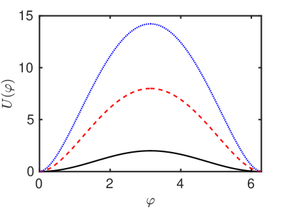
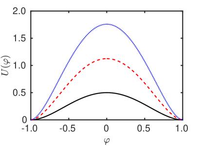
Figure 2: The nonlinear Klein-Gordon potentials are shown. Left-hand panel: $l=1$ (solid black line), $l=3$ (numerical results, dashed red line), and $l=5$ (numerical results, dotted blue line). Right-hand panel: $l=2$ (solid black line), $l=4$ (dashed red line), and $l=6$ (numerical results, dotted blue line).

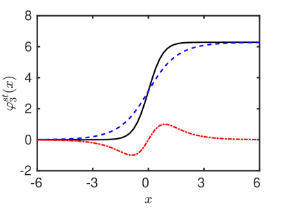
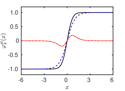
Figure 3: Left-hand and right-hand panels show the kinks (solid black line), represented by Eq. (4.3) for $l=3$ and $l=4$, respectively. This solution is a linear superposition of a kink (dashed blue line) and a localized function (dot-dashed red line).

Finally, let us consider the case of $l=4$. We set $Q=2$, and $C_{-}=-1$, which imply $\alpha=2^{3/8}/3^{1/4}$, and $C_{+}=1$. Equation (4.9), using Eqs.  (4.10) and (4.12), can be solved explicitly, and the potential, for $|\varphi^{st}(x)|\leq 1$, has the form (see Fig. 2)

$$U[\varphi^{st}(x)]=\frac{9}{8}\left[1-2\cos\left(\frac{2}{3}\arcsin\varphi^{st}(x)\right)\right]^{4}.$$ (4.15)

From Eq. (4.3), its kink solution

$$\varphi^{st}(x)=\tanh(x)+\frac{1}{2}\,\frac{\tanh(x)}{\cosh^{2}(x)}$$ (4.16)

is a linear superposition of two functions, the first one is the $\varphi^{4}$ kink, and the second one is a localized function (see right-hand panel of Fig. 3). Since $l=4$, the lower phonon frequency equals $\omega_{ph}=l=4$, and the $4$ discrete modes are related with the frequencies $\omega_{\kappa}=\sqrt{\omega_{ph}^{2}-\kappa^{2}}$, that is, $\omega_{1}=\sqrt{15}$, $\omega_{2}=\sqrt{12}$, $\omega_{3}=\sqrt{7}$, and $\omega_{4}=0$. Moreover, according to the results of the previous section, this kink is also stable.

Notice that the formula (4.9) defines the Klein-Gordon potentials $U(\varphi)$, which can be explicitly expressed for a few particular cases. From (4.9) and (4.10), it can be shown that, for all odd values $l\geq 3$, it is impossible to find an explicit expression for $U$ since the functions $\arcsin z$ and $\sqrt{1-z}$, where $z=\alpha^{2}U^{1/l}$, appear in different terms of the same equation. A similar situation happens when $l$ is an even number greater than $4$, since, in this case, the explicit solution is involved with the roots of a polynomial in $U$ of degree equal to or greater than $5$, which are, in general, impossible to obtain analytically. Therefore, for $l\geq 6$, the stable kink solution is represented by Eq. (4.3), whereas its corresponding Klein-Gordon potential can be numerically obtained by solving Eq. (4.9), and specifying the topological charge $Q$ and the constant $C_{-}$.

As a final remark it is important to point out the fact that Eq. (4.7) was obtained in Ref. [71] by differentiation of the positive branch of Eq. (4.8). Since the authors analyzed the first correction to the masses of a family of nonlinear Klein-Gordon kinks, rather than provide the solution of the differential equation for the potential, they calculated the kink’s mass (1.1) by using the Bogomolnyi equation. They obtained $M_{l}=24^{l-1}\Gamma^{2}(l)/\Gamma(2\,l)$, which differs from the expression (4.4) due to a different choice of the normalization constant $A_{l}$ in Eq. (4.2). Here, $A_{l}$ is given by Eq. (4.2) such that $Q=2$ for even values of $l$, whereas in Ref. [71], $A_{l}$ equals $1$ for all values of $l$.

4.2 The lowest eigenvalue is negative

The second case deals with negative values of $\omega_{l}^{2}$, thus the solitary wave is linearly unstable. Let us assume that the static pulse solution of the nonlinear Klein-Gordon has the form

$$\phi^{st}(x)=\frac{1}{\cosh^{n}(x)},$$ (4.17)

where the parameter $n$ is determined a posteriori. Using the relationship (2.15), this condition implies that

$$U(\phi)=\frac{n^{2}}{2}\phi^{2}\left(1-\phi^{2/n}\right).$$ (4.18)

The envelope part of the NLS soliton with arbitrary power-law nonlinearity $|\Psi(x)|^{2/n}$ is represented by Eq. (4.17) since it satisfies the nonlinear Klein-Gordon equation (1.2), where the potential is given by Eq. (4.18) [53]. However, the stability of the NLS soliton is determined by a more complex eigenvalue problem than that represented by Eq. (3.1), see Chapter 4 of Ref. [53]. The investigation of the stability of the solution (4.17) leads to the Sturm-Lioville problem (3.1), where $U^{\prime\prime}(\phi)=n^{2}-(n+1)(n+2)\phi^{2/n}$. By comparing this expression with Eqs. (3.2)-(3.4), we obtain $n=l-1$, and $\omega_{ph}^{2}=(l-1)^{2}$ ($l\geq 2$). From the above analysis, the discrete frequencies are represented by $\omega_{\kappa}^{2}=\omega_{ph}^{2}-\kappa^{2}$, where $\kappa=1,2,\cdots,l$. Clearly, the frequency $\omega_{l}^{2}=(l-1)^{2}-l^{2}<0$ and all pulses (4.17) are unstable. The question therefore arises as to whether there is any way to stabilize the pulses.

5 Control of stability

The purpose of this section is to obtain stable pulses, associated to the nonlinear Klein-Gordon potential, with the help of an inhomogeneous force $f(x)$. A similar procedure has been successfully considered in Refs. [72, 73] to control the existence of internal modes associated to topological solitons in the perturbed $\varphi^{4}$-potential and in the inhomogeneous sine-Gordon equation. For instance, let’s consider the following nonlinear Klein-Gordon equation with an external force

$$\phi_{tt}-\phi_{xx}+\frac{dU}{d\phi}=f(x),$$ (5.1)

where $U$ is the $\phi^{3}$ potential given by Eq. (4.18) by setting $n=2$. The unstable static pulse solution, when $f(x)=0$, has the form $\phi^{st}(x)=1/\cosh^{2}(x)$. Straightforward calculations show that the pulse

$$\phi(x)=a\,\phi^{st}(b\,x),$$ (5.2)

with positive constants $a$ and $b$, is the solution of Eq. (5.1) whenever

$$f(x)=\frac{2a}{\cosh^{4}(bx)}\left[1-3\,a+2b^{2}+(1-b^{2})\cosh(2bx)\right].$$ (5.3)

In order to study the stability of the pulse (5.2), the methodology of Section 2 is applied. Hence, Eq. (5.1) is linearized around the pulse, that is, the expansion (2.11) is inserted in Eq. (5.1). The function $\Psi(x,t)$ satisfies Eq. (2.12). Finally, by assuming the ansatz (2.13), the function $\psi(x)$ satisfies the Sturm-Liouville problem (2.14).

By inserting the pulse (5.2) into the second derivative of the potential, it has the form

$$U^{\prime\prime}[\phi(x)]=4-\frac{12\,a}{\cosh^{2}(b\,x)}.$$ (5.4)

By assuming the change of variable $X=b\,x$, the Sturm-Liouville problem reads

$$\psi_{XX}+\left[\frac{\omega^{2}}{b^{2}}-\frac{4}{b^{2}}+\frac{12\,a}{b^{2}\,\cosh^{2}(X)}\right]\psi=0.$$ (5.5)

For certain values of $a$ and $b$, the $\mathop{\rm sech}^{2}(x)$ potential becomes the Pöschl-Teller potential, that is,

$$\frac{12\,a}{b^{2}}=l\,(l+1).$$ (5.6)

There are two different ways to stabilize the pulse. To start with, the value of $b$ is fixed, for instance as $b=1$. This implies that the lowest phonon frequency is $\omega_{ph}=2$. The discrete set of frequencies is given by

$$\omega^{2}=\omega_{ph}^{2}-\kappa^{2},$$

where $\kappa=1,2,\cdots,l$. Demanding stability, all values of $\omega^{2}$ should be non-negative. This implies that $\min(\omega^{2})=4-l^{2}\geq 0$, i.e. either $l=1$ ($a=1/6$) or $l=2$ ($a=1/2$). In particular, the discrete mode for the case $l=1$ reads

$$\psi_{1}(x)=e^{-x}P_{1}^{(1,-1)}(\tanh x)=\frac{1}{\cosh(x)},\qquad\omega_{1}^{2}=3,$$ (5.7)

while the continuous spectrum is represented by

$$\psi_{k}(x) = e^{ikx}\,[\tanh(x)-i\,k],\qquad\omega_{k}^{2}=4+k^{2}.$$ (5.8)

For the case $l=2$ ($a=1/2$), the solution of the Sturm-Liouville problem is represented by the expressions (3.33), (3.34), and (3.35). Hence, the two pulses considered are stable.

The second method to stabilize the pulse is to set $a$, for instance $a=1/3$, and to change $b$ in accordance with Eq. (5.6), where now $4/b^{2}=l\,(l+1)$. In this case, the lowest phonon frequency changes with $b$, that is, $\omega_{ph}=2/b$. By imposing the condition $\omega^{2}\geq 0$ for all frequencies, we obtain that the integer number $l^{2}\leq 4/b^{2}$. This inequality is satisfied by all integer values of $l$ ($b=2/\sqrt{l\,(l+1)}$). For instance, if $l=1$, then the value of $b=\sqrt{2}$. If $l=2$, then the value of $b=\sqrt{2/3}$. As $l$ is increased, the number of discrete modes grows, $b$ decreases, and the stable pulse becomes broader.

6 Conclusions

The stability of kinks and pulses of the nonlinear Klein-Gordon Eq. (1.2) is investigated by the following procedure: (i) It is assumed that its general solution (2.11) is the superposition of the static solution plus a small perturbation, which depends not only on space, but also on time; (ii) By substituting this ansatz in Eq. (1.2), the partial differential equation (2.12) that governs the perturbation is obtained; (iii) The solution of this equation leads to a Sturm-Liouville problem (3.1), which is solved in a systematic way for the Pöschl-Teller potential $-l\,(l+1)\,\mathop{\rm sech}^{2}(x)$, $l\in\mathbb{N}$.

The detailed resolution of the Sturm-Liouville problem (3.1) shows that its real eigenvalues are equal to $\omega^{2}=\omega_{ph}^{2}+k^{2}$ (squared eigenfrequencies), where $\omega_{ph}$ is the lowest frequency of the continuous spectrum, and $k^{2}\in\mathbb{R}$. For $k\geq 0$, we obtain the frequencies of the continuous spectrum $\omega(k)=\sqrt{\omega_{ph}^{2}+k^{2}}$. Considering $k=i\kappa$, with $\kappa\in\mathbb{R}$, we obtain the frequencies of the discrete spectrum, $\omega_{\kappa}=\sqrt{\omega_{ph}^{2}-\kappa^{2}}$. The eigenfunctions of the Sturm-Liouville problem, up to a normalizing constant, are $\psi(x)=\exp^{ikx}\,P_{l}^{(-ik,ik)}[\tanh(x)]$, where $P_{l}^{(-ik,ik)}[\tanh(x)]$ are the Jacobi polynomials. Interestingly, the degree of the polynomial, $l$, determines the number of discrete modes, and the parameter $\kappa$ takes the values from $1$ to $l$ so that the solution of the Sturm-Liouville problem is bounded.

Furthermore, we establish the orthogonality and completeness relations of this set of eigenfunctions for all values of $l\in\mathbb{N}$. These results, mentioned in Ref. [37] for $l=1$ and in Ref. [68] for $l=2$, rigorously justify that the solutions of perturbed nonlinear Klein-Gordon equations can be written as an expansion in the set of these eigenfunctions.

Starting from the Pöschl-Teller potential and using the fact that the translational mode is proportional to the spatial derivative of the kink, we obtain a family of nonlinear Klein-Gordon potentials. Our procedure has two advantages with respect to the previous studies in Refs. [48, 49]. First, our analysis is valid for all values of $l$ and the solution of the second-order differential equation for $U(\varphi)$ is represented in a closed form by Eq. (4.9) in terms of the hypergeometric function, where $l$ is a parameter. Second, our approach shows that the sine-Gordon and $\varphi^{4}$ kinks are at the bottom of the hierarchy of stable kinks associated with a certain class of nonlinear Klein-Gordon potentials.

For the values of $l=1$ and $l=2$, the spectrum related to the sine-Gordon and $\varphi^{4}$ equations, respectively, are recovered [37, 22]. Furthermore, we show that, for $l>2$, there is a family of kinks corresponding to Klein-Gordon potentials. The potential for $l=4$ is obtained explicitly, whereas for $l=3$ and $l\geq 5$, the potentials can be expressed implicitly. Interestingly, we analytically obtain the kink solutions Eq. (4.3) even when the potential can only be numerically found. The kinks are stable, and are a linear superposition of two terms: the first is either the sine-Gordon kink (for $l$ odd numbers) or the $\varphi^{4}$ kink (for even $l$), while the second is a localized function. These kinks resemble the $\varphi^{4}$ wobbling kinks studied in Ref. [11]. The corresponding spectra of the Sturm-Liouville problem associated to the stability of these kinks have several internal modes, some of which have a localized odd eigenfunction, while others have a localized even eigenfunction.

Finally, we found that if the lowest frequency of the continuous spectrum satisfies $\omega_{ph}<l$ (sufficient condition for instability), then the static solution is unstable. This is precisely the case of all the studied pulses $\mathop{\rm sech}^{n}(x)$ of a family of nonlinear Klein-Gordon equations with a potential given by Eq. (4.18). We explain how certain inhomogeneous terms can be introduced into the nonlinear Klein-Gordon equation in order to obtain stable pulses.

To complete our discussion, the following observations are in order:

1. Not all Sturm-Liouville problems associated to the stability problem of the nonlinear Klein-Gordon equation lead to the Pöschl-Teller potential (see, for instance, Ref. [23, 74]).

2. Not all the Sturm-Liouville problems associated with the linear stability of static solutions of the nonlinear Klein-Gordon equations have been analytically solved. For instance, for the double sine-Gordon equation [21, 6], only its kink solution and the zero mode of its associated Sturm-Liouville problem are known. Indeed, by taking the spatial derivative of its static kink, it has no zeros. According to our results, all the remaining discrete eigenvalues, if any, are positive, and the double sine-Gordon kink is linearly stable. However, the computation of the explicit expressions for the remaining eigenfunctions remains an open problem.

Appendix A The orthogonality and completeness relations

In this section, the orthogonality and completeness relations presented in Section 3.3 are deduced. In order to achieve our goal, the theory of the one-dimensional Schrödinger equation, developed in Chapter 3§2 of Ref. [54], is employed.

Instead of dealing with the function $\psi(x,k)$ given by (3.10) and $\psi(x,-k)$, it is convenient to use the functions $u_{1}(x,k)$ and $u_{2}(x,k)$, defined below (see Eq. (A.3)). First, two independent solutions of Eq. (3.1) are introduced, the so-called Jost functions,

$$f_{1}(x,k) = \frac{\psi(x,k)}{P_{l}^{(-ik,ik)}(1)},$$

$$f_{2}(x,k) = \frac{\psi(x,-k)}{P_{l}^{(ik,-ik)}(-1)},\quad k>0,$$ (A.1)

with the asymptotics

$$f_{1}(x,k) = e^{ikx}+o(1)\mbox{ as }x\to\infty,$$

$$f_{2}(x,k) = e^{-ikx}+o(1)\mbox{ as }x\to-\infty.$$ (A.2)

Subsequently, using Eq. (2.12) on page 159 of Ref.[54], the transmission coefficient $a(k)$ is defined,

$$a(k):=\frac{1}{2ki}W[f_{1}(x,k),f_{2}(x,k)]=-\frac{A_{l,k}^{2}}{P_{l}^{(-ik,ik)}(1)P_{l}^{(ik,-ik)}(-1)},$$

for $k>0$, where $A_{l,k}$ is given by Eq. (3.15). According to Theorem 2.3 on page 165 in Ref. [54], the new functions

$$u_{\ell}(x,k) = \frac{f_{\ell}(x,k)}{a(k)},\quad\ell=1,2,\quad k>0,$$

$$u_{\ell}(x,0) = P^{(0,0)}_{l}(\tanh x),$$ (A.3)

together with the eigenfunctions corresponding to the discrete spectrum (3.25), constitute an orthogonal complete set of functions in $L^{2}(\mathbb{R})$. The orthogonality reads

$$\int_{\mathbb{R}}\psi_{\kappa}(x)\psi_{\nu}(x)dx=\delta_{\kappa,\nu},\quad\int_{\mathbb{R}}\psi_{\kappa}(x){u_{\ell}(x,k)}dx=0,\quad$$ (A.4)

$$\frac{1}{2\pi}\int_{\mathbb{R}}\overline{u_{\ell}(x,k)}u_{\iota}(x,m)dx=\delta_{\ell,\iota}\delta(k-m),$$ (A.5)

where $\nu,\kappa=1,2\ldots,l$; $\ell,\iota=1,2$; $k,m\geq 0$; $\delta_{\kappa,\nu}$ is the Kronecker delta, and $\delta(x)$ denotes the delta Dirac function (which is not actually a function, but a distribution, and hence Eq. (A.5) should be understood in the distributional sense). For an introduction to the theory of distribution see e.g. Ref. [75].

On the other hand, for all $\Phi(x)\in L^{2}(\mathbb{R})$, one has the expansion [54]. Recall that Eq. (2.25), on page 165 of Ref. [54], which is a completeness relation, is proved for $\Phi\in C_{0}^{2}(\mathbb{R})$ (twice continuously differentiable functions on $\mathbb{R}$ with compact support). However, since $C_{0}^{\infty}(\mathbb{R})$ (infinitely differentiable functions on $\mathbb{R}$ with compact support) is a subset of $C_{0}^{2}(\mathbb{R})$ and $C_{0}^{\infty}(\mathbb{R})$ is dense in $L^{2}(\mathbb{R})$, then $C_{0}^{2}(\mathbb{R})$ is dense in $L^{2}(\mathbb{R})$ and therefore the following expansion is true for all $\Phi\in L^{2}(\mathbb{R})$

$$\Phi(x)= \displaystyle\frac{1}{2\pi}\displaystyle\sum_{\ell=1}^{2}\!\int_{0}^{\infty}\!\!c_{\ell}(k)u_{\ell}(x,k)dk+\displaystyle\sum_{\kappa=1}^{l}c_{\kappa}\psi_{\kappa}(x),$$ (A.6)

where

$$c_{\ell}(k) = \int_{\mathbb{R}}\overline{u_{\ell}(y,k)}\Phi(y)dy,$$

$$c_{\kappa} = \int_{\mathbb{R}}\psi_{\kappa}(y)\Phi(y)dy.$$

Formula (A.6) is the so-called completeness relation for the set $\{u_{1},u_{2}\}_{k\geq 0}\cup\{\psi_{\kappa}\}_{\kappa=1,\ldots,l}$. It can also be written in the distributional sense as follows (see Remark on page 168 in Ref. [54]):

$$\int_{0}^{\infty}\sum_{\ell=1}^{2}\left[u_{\ell}(x,k)\overline{u_{\ell}(y,k)}\right]dk+\sum_{\kappa=1}^{l}\psi_{\kappa}(x)\psi_{\kappa}(y)=\delta(x-y).$$ (A.7)

The above orthogonality and completeness relations can be written in a compact form. Notice that the integrands of the first terms in Eq. (A.6) are

$$c_{\ell}(k)u_{\ell}(x,k)=\left(\int_{0}^{\infty}\overline{u_{\ell}(y,k)}\Phi(y)dy\right)u_{\ell}(x,k),\qquad\ell=1,2.$$

Using $|P_{l}^{(ik,-ik)}(-1)|^{2}=|P_{l}^{(-ik,ik)}(1)|^{2}=A_{l,k}^{2}$, it is straightforward to deduce that

$$\overline{u_{1}(y,k)}u_{1}(x,k) = \frac{\overline{\psi(y,k)}\psi(x,k)}{A_{l,k}^{2}},$$

$$\overline{u_{2}(y,k)}u_{2}(x,k) = \frac{\overline{\psi(y,-k)}\psi(x,-k)}{A_{l,k}^{2}}.$$

Using the above identities and changing $k\to-k$ in the second integral of Eq. (A.6), this expression becomes

$$\Phi(x)= \displaystyle\frac{1}{2\pi}\int_{\mathbb{R}}\left[A_{l,k}^{-2}\left(\int_{\mathbb{R}}\overline{\psi(y,k)}\Phi(y)dy\right)\psi(x,k)\right]dk$$

$$\qquad\displaystyle+\sum_{\kappa=1}^{l}\left(\int_{\mathbb{R}}\psi_{\kappa}(y)\Phi(y)dy\right)\psi_{\kappa}(x).$$

From the above equation it follows that the set of functions defined by Eqs. (3.25)-(3.26) satisfies the completeness relation (3.27) and its equivalent expression (3.28). In a similar way the orthogonality relations (A.4)-(A.5) become the relations (3.29)-(3.30), respectively.

The set of functions defined by Eqs. (3.25) and (3.26) that satisfy the relations (3.28), (3.29), and (3.30) are those used in the theory of the nonlinear Klein-Gordon Eq. (1.2).

References

- [1] B. S. Getmanov. Soliton Bound States in the in Two-Dimensions Field Theory. Pisma Zh. Eksp. Teor. Fiz., 24:323, 1976.
- [2] V. G. Makhankov. Dynamics of classical solitons (in non-integrable systems). Phys. Rep., 35:1, 1978.
- [3] T. Sugiyama. Kink-Antikink Collisions in the Two-Dimensional Model. Prog. Theor. Phys., 61:1550, 1979.
- [4] S. Aubry. A unified approach to the interpretation of displacive and order-disorder systems. II. Displacive systems. J. Chem. Phys., 64:3392, 1976.
- [5] D. K. Campbell, J. F. Schonfeld, and C. A. Wingate. Resonance structure in kink-antikink interactions in theory. Phys. D: Nonlinear Phenomena, 9:32, 1983.
- [6] D. K. Campbell, M. Peyrard, and P. Sodano. Kink-antikink interactions in the double sine-Gordon equation. Phys. D: Nonlinear Phenomena, 19:165, 1986.
- [7] P. Dorey, K. Mersh, T. Romanczukiewicz, and Y. Shnir. Kink-Antikink Collisions in the Model. Phys. Rev. Lett., 107:091602, 2011.
- [8] A. Demirkaya, R. Decker, P. G. Kevrekidis, I. C. Christov, and Saxena A. Kink dynamics in a parametric system: A model with controllably many internal modes. J. High Energy Phys., 12:071, 2017.
- [9] D. K. Campbell. Historical Overview of the Model. In Panayotis G. Kevrekidis and Jesús Cuevas-Maraver, editors, A Dynamical Perspective on the Model: Past, Present and Future, pages 1–22. Springer International Publishing, Cham, 2019.
- [10] I. V. Barashenkov and O. F. Oxtoby. Wobbling kinks in theory. Phys. Rev. E, 80:026608, 2009.
- [11] I. V. Barashenkov. The Continuing Story of the Wobbling Kink. In Panayotis G. Kevrekidis and Jesús Cuevas-Maraver, editors, A Dynamical Perspective on the Model: Past, Present and Future, pages 187–212. Springer International Publishing, Cham, 2019.
- [12] L. D. Landau. On the theory of phase transitions. Zh. Eksp. Teor. Fiz., 7:19, 1937.
- [13] L. D. Landau and V. L. Ginzburg. On the theory of superconductivity. Zh. Eksp. Teor. Fiz., 20:1064, 1950.
- [14] A. Khare, I. C. Christov, and A. Saxena. Successive phase transitions and kink solutions in , , and field theories. Phys. Rev. E, 90:023208, 2014.
- [15] F. J. Buijnsters, A. Fasolino, and M. I. Katsnelson. Motion of Domain Walls and the Dynamics of Kinks in the Magnetic Peierls Potential. Phys. Rev. Lett., 113:217202, 2014.
- [16] I. C. Christov, R. J. Decker, A. Demirkaya, V. A. Gani, P. G. Kevrekidis, A. Khare, and A. Saxena. Kink-Kink and Kink-Antikink Interactions with Long-Range Tails. Phys. Rev. Lett., 122:171601, 2019.
- [17] A. Saxena, I. C. Christov, and A. Khare. Higher-Order Field Theories: , and Beyond. In Panayotis G. Kevrekidis and Jesús Cuevas-Maraver, editors, A Dynamical Perspective on the Model: Past, Present and Future, pages 253–279. Springer International Publishing, Cham, 2019.
- [18] H. Goldstein. Classical Mechanics (3rd ed.). San Francisco, CA:, Addison Wesley, 1980.
- [19] W. C. Fullin. One-dimensional field theories with odd-power self-interactions. Phys. Rev. D, 18:1095, 1978.
- [20] A. C. Scott. A Nonlinear Klein-Gordon Equation. Am. J. Phys., 37:52, 1969.
- [21] C. A. Condat, R. A. Guyer, and M. D. Miller. Double sine-Gordon chain. Phys. Rev. B, 27:474, 1983.
- [22] R. F. Dashen, B. Hasslacher, and A. Neveu. Nonperturbative methods and extended-hadron models in field theory. II. Two-dimensional models and extended hadrons. Phys. Rev. D, 10:4130, 1974.
- [23] M. A. Lohe. Soliton structures in . Phys. Rev. D, 20:3120, 1979.
- [24] Th. Dauxois and M. Peyrard. Physics of Solitons. Cambridge University Press, Cambridge, 2006.
- [25] B. A. Malomed. The sine-Gordon Model: General Background, Physical Motivations, Inverse Scattering, and Solitons. In Jesús Cuevas-Maraver, Panayotis G. Kevrekidis, and Floyd Williams, editors, The sine-Gordon Model and its Applications, pages 1–30. Springer International Publishing, Cham, 2014.
- [26] A. Barone, F. Esposito, C. J. Magee, and A. C. Scott. Theory and applications of the sine-Gordon equation. La Rivista del Nuovo Cimento, 1:227, 1971.
- [27] I. V. Barashenkov, M. M. Bogdan, and V. I. Korobov. Stability Diagram of the Phase-Locked Solitons in the Parametrically Driven, Damped Nonlinear Schrödinger Equation. Europhys. Lett., 15:113, 1991.
- [28] Yu. S. Kivshar, Z. Fei, and L. Vázquez. Resonant soliton-impurity interactions. Phys. Rev. Lett., 67:1177, 1991.
- [29] M. Salerno and Y. Zolotaryuk. Soliton ratchetlike dynamics by ac forces with harmonic mixing. Phys. Rev. E, 65:056603, 2002.
- [30] L. Morales-Molina, N. R. Quintero, F. G. Mertens, and A. Sánchez. Internal Mode Mechanism for Collective Energy Transport in Extended Systems. Phys. Rev. Lett., 91:234102, 2003.
- [31] A. V. Ustinov, C. Coqui, A. Kemp, Y. Zolotaryuk, and M. Salerno. Ratchetlike Dynamics of Fluxons in Annular Josephson Junctions Driven by Biharmonic Microwave Fields. Phys. Rev. Lett., 93:087001, 2004.
- [32] N. R. Quintero. Soliton ratchets in sine-Gordon-like equations. In Jesús Cuevas-Maraver, Panayotis G. Kevrekidis, and Floyd Williams, editors, The sine-Gordon Model and its Applications, pages 131–154. Springer International Publishing, Cham, 2014.
- [33] N. Casic, N. Quintero, R. Alvarez-Nodarse, F. G. Mertens, L. Jibuti, W. Zimmermann, and T. M. Fischer. Propulsion Efficiency of a Dynamic Self-Assembled Helical Ribbon. Phys. Rev. Lett., 110:168302, 2013.
- [34] A. C. Scott. Nonlinear Science. Oxford University, Oxford, 1999.
- [35] A. C. Scott. Waveform stability on a nonlinear Klein-Gordon equation. Proc. IEEE, 57:1338, 1969.
- [36] R. D. Parmentier. Stability analysis of neuristor waveforms. Proceedings of the IEEE, 55:1498, 1967.
- [37] J. Rubinstein. Sine-Gordon Equation. J. Math. Phys., 11:258, 1970.
- [38] R. J. Buratti and A. G. Lindgren. Neuristor waveforms and stability by the linear approximation. Proceedings of the IEEE, 56:1392, 1968.
- [39] P. M. Morse and H. Feshbach. Methods of theoretical Physics, volume 2. 1953.
- [40] G. Pöschl and E. Teller. Bemerkungen zur Quantenmechanik des anharmonischen Oszillators. Z. Physik, 83:143, 1933.
- [41] P. S. Epstein. Reflexion of waves in an inhomogeneous absorbing medium. Proc. Natl. Acad. Sci. USA., 16:627, 1930.
- [42] C. Eckart. The penetration of a potential barrier by electrons. Phys. Rev., 35:1303, 1930.
- [43] P. M. Morse and H. Feshbach. Methods of theoretical Physics, volume 1. McGraw-Hill, New York, 1953.
- [44] S. Flügge. Practical Quantum Mechanics. Springer-Verlag, Berlin, 1994.
- [45] L. D. Landau and E. M. Lifshitz. Quantum Mechanics. Pergamon Press, Oxford, 3th edition, 1977.
- [46] P. G. Drazin and R. S. Johnson. Solitons: An Introduction. Cambridge University Press, Cambridge, 1989.
- [47] J. Yang. Complete eigenfunctions of linearized integrable equations expanded around a soliton solution. J. Math. Phys., 41:6614, 2000.
- [48] N. H. Christ and T. D. Lee. Quantum expansion of soliton solutions. Phys. Rev. D, 12:1606, 1975.
- [49] S. E. Trullinger and R. J. Flesch. Parent potentials for an infinite class of reflectionless kinks. J. Math. Phys, 28:1683, 1987.
- [50] P. J. Hansen and D. R. Nicholson. Simple soliton solutions. Am. J. Phys., 47:769, 1979.
- [51] D. J. Korteweg and G. de Vries. On the change of form of long waves advancing in a rectangular canal, and on a new type of long stationary waves. The London, Edinburgh, and Dublin Philosophical Magazine and Journal of Science, 39:422, 1895.
- [52] R. Y. Chiao, E. Garmire, and C. H. Townes. Self-Trapping of Optical Beams. Phys. Rev. Lett., 13:479, 1964.
- [53] C. Sulem and P. L. Sulem. The nonlinear Schrödinger equation. Self-focusing and wave collapse. . Springer-Verlag, New York, 1999.
- [54] L. A. Takhtajan. Quantum mechanics for mathematicians. Graduate Studies in Mathematics, 95. American Mathematical Society, Providence, R.I., 2008.
- [55] E. B. Bogomolnyi. Stability of classical solutions. Sov. J. Nucl. Phys., 24:449, 1976.
- [56] N. Manton and P. Sutcliffe. Topological Solitons. Cambridge Monographs on Mathematical Physics. Cambridge University Press, 2004.
- [57] J. Goldstone and R. Jackiw. Quantization of nonlinear waves. Phys. Rev. D, 11:1486, 1975.
- [58] W. Eckhaus. Studies in Non-Linear Stability Theory. Springer-Verlag, Berlin Heidelberg, 1965.
- [59] G. Szegö. Orthogonal Polynomials. Fouth Edition. American Mathematical Society, Colloquium Publications Vol. XXIII, Providence, R.I., 1975.
- [60] P. Rusev. Classical orthogonal polynomials and their associated functions in complex domain. Bulgarian Mathematical Monographs 10, Prof. Marin Drinov Acad. Publ. House, Sofia, Bulgaria, 2005.
- [61] F. W. J. Olver, D. W. Lozier, R. F. Boisvert, and C. W. Clark May, editor. NIST Handbook of Mathematical Functions Paperback and CD-ROM. Cambridge University Press, New York, 2010.
- [62] V. I. Arnold. Ordinary differential equations. Second printing of the 1992 edition. Universitext. Springer-Verlag, Berlin, 2006.
- [63] G. F. Simmons. Differential Equations With Applications and Historical Notes. McGraw-Hill Education, 2º Ed, 1991.
- [64] M. B. Fogel, S. E. Trullinger, A. R. Bishop, and J. A. Krumhansl. Dynamics of sine-Gordon solitons in the presence of perturbations. Phys. Rev. B, 15:1578, 1977.
- [65] M. M. Bogdan and A. M. Kosevich and V. P. Voronov. Generation of the internal oscillation of soliton in a one-dimensional non-integrable system. In V. G. Makhankov and V. K. Fedyanin and O. K. Pashaev, editor, Proceedings of IVth International Workshop “Solitons and Applications”, pages 397–401. World Scientific, Part IV, Singapore, 1990.
- [66] P. G. Kevrekidis. Integrability revisited: a necessary condition. Phys. Lett. A, 285:383, 2001.
- [67] O. V. Charkina and M. M. Bogdan. Internal Modes of Solitons and Near-Integrable Highly-Dispersive Nonlinear Systems. Symmetry, Integr. Geom.:Methods Appl., 2:047, 2006.
- [68] A. R. Bishop, J. A. Krumhansl, and S. E. Trullinger. Solitons in condensed matter: A paradigm. Phys. D: Nonlinear Phenomena, 1:1, 1980.
- [69] E. Magyari. Direct linear stability analysis for solitary waves. Phys. Rev. A, 31:1174, 1985.
- [70] D. E. Amos. Representations of the central and non-central distributions. Biometrika, 51:451, 1964.
- [71] L. J. Boya and J. Casahorran. Quantum masses for a general family of bidimensional kinks. Phys. Rev. D, 41:1342, 1990.
- [72] J. A. González, B. A. Mello, L. I. Reyes, and L. E. Guerrero. Resonance Phenomena of a Solitonlike Extended Object in a Bistable Potential. Phys. Rev. Lett., 80:1361, 1998.
- [73] J. A. González, A. Bellorín, M. A. García-Ñustes, L. E. Guerrero, S. Jiménez, and L. Vázquez. Arbitrarily large numbers of kink internal modes in inhomogeneous sine-Gordon equations. Phys. Lett. A, 381:1995, 2017.
- [74] I. V. Barashenkov and V. G. Makhankov. Soliton-like “bubbles” in a system of interacting bosons. Phys. Lett. A, 128:52, 1988.
- [75] R. Strichartz. A guide to distribution theory and Fourier transforms. Studies in Advanced Mathematics. CRC Press, Boca Raton, FL, 1994.