Neural interval-censored Cox regression with feature selection

Abstract

The classical Cox model emerged in 1972 promoting breakthroughs in how patient prognosis is quantified using time-to-event analysis in biomedicine. One of the most useful characteristics of the model for practitioners is the interpretability of the variables in the analysis. However, this comes at the price of introducing strong assumptions concerning the functional form of the regression model. To break this gap, this paper aims to exploit the explainability advantages of the classical Cox model in the setting of interval-censoring using a new Lasso neural network that simultaneously selects the most relevant variables while quantifying non-linear relations between predictors and survival times. The gain of the new method is illustrated empirically in an extensive simulation study with examples that involve linear and non-linear ground dependencies. We also demonstrate the performance of our strategy in the analysis of physiological, clinical and accelerometer data from the NHANES 2003-2006 waves to predict the effect of physical activity on the survival of patients. Our method outperforms the prior results in the literature that use the traditional Cox model.

Keywords Survival analysis; Interval-censoring; Neural nets; Cox model; High-dimensional statistics

1 Introduction

In recent decades, interval-censored data modeling has been a subject of intense research from methodological, theoretical, and applied perspectives (van de Geer, 1993; Huang 1996; Wu and Cook 2020; Cho et al. 2021). Recently, the first machine learning contributions appeared in the literature as specific smoothing random forest algorithms (Cho et al. (2021)), a more classical tree ensemble random forest (Yao et al. (2019)) or the first methodology tackling interval-censoring based on kernel machines (Travis-Lumer and Goldberg (2021)). Notably, to the best of our knowledge, deep learning algorithms is missing in this setting, despite the recent progress this field has had during the last years with right-censored outcomes (Rindt et al. (2022)), in estimating the conditional survival function (Zhong et al. (2021); Lee et al. (2018); Steingrimsson and Morrison (2020)) or the conditional quantiles (Jia and Jeong (2022)).

Despite the progress achieved, further research on developing non-linear regression models to handle general dependence relationships between predictors and time events is needed. Also, model complexity ought to be reduced through simultaneous variable selection. The first contributions in the mentioned direction have recently appeared in both areas (Gao et al. 2019; Li et al. 2020), but in the context of classical Cox models arbitrary relations of dependence are not addressed.

In order to address this challenge, linear penalized regression models constitute the primary benchmark for simultaneously predictive tasks and variable selection. In this context, the Lasso (Least Absolute Shrinkage and Screening Operator) is maybe the most popular method in the literature ((Tibshirani, 1996, 1997)). However, despite its wide use by practitioners, their behavior can be suboptimal in several situations, especially in scenarios involving dependence among predictors ((Bühlmann and Van De Geer,, 2011; Bertsimas et al., 2020; Freijeiro-González et al., 2022)).

Given the need to expand the Lasso models to other settings, multiple extensions of Lasso have been proposed in the literature, together with other penalized regression or variable selection models that combine penalty functions of convex and non-convex nature such as SCAD or, more recently, with the $\ell_{0}$ norm. In the last case, the advances in integer programming (Bertsimas et al., 2016) and gradient-based optimization (Hazimeh and Mazumder, 2020; Bertsimas et al., 2020) may lead to new directions for efficient variable selection in large and high dimensional data.

Adopting these penalized regression methods for more general dependence relations between predictors and responses is more limited. Advances in additive models (GAM) (Huang et al., 2010) or the new neural network with feature sparsity LassoNet are noteworthy (Lemhadri et al., 2021).

This paper aims to exploit the advantages of the new LassoNet in interval-censoring mechanisms to tackle non-linear regression of time outcomes for the first occasion in statistical literature. All while keeping the interpretability advantages of the classical Cox model, which enables representation of individual predictors’ risk in terms of hazard functions.

The analysis of interval-censored data is an important and relevant problem in medicine or, more specifically, in personalized medicine applications. In practice, disease diagnoses occur between two known time instants that correspond to two medical visits, such as the diagnosis of diabetes mellitus disease or the onset of a tumour. Consequently, from a mathematical point of view, the problem of quantifying the prognostic of patients is formalized as a regression model in which the response is subject to interval-censoring.

In this paper we analyze the NHANES 2003-2006 physical activity data, which incorporates monthly mortality checks, to show the advantages of our method over other existing regression models in the literature. In this sense, we can state our problem as predicting survival functions. Several papers have performed survival analysis with these data, but only from a linear perspective with the traditional Cox model (McGregor et al., 2020; Smirnova et al., 2020). However, we use for the first time a non-linear approach while simultaneously selecting the most critical variables. Our analysis leads to powerful findings because the exercise-response dose follows a non-linear relationship according to the physical activity literature. At the same time, our approach presents the advantages of interpreting the effect of covariates thanks to Cox model’s semiparametric structure.

The structure of the paper is as follows: Section 2 introduces the mathematical details of the new algorithm with the latest optimization strategy. Then, Section 3 presents an intensive simulation study that involves non-linear and linear regression models, where we show empirically the advantages of our approach. Next, Section 4 motivates an application to physical activity data from NHANES and draws the results of this example. Finally, in Section 5, we discuss our proposal’s potential in biomedicine and also from a methodological point of view.

2 Methods

2.1 Statistical model

Let $T\in\left[0,+\infty\right)$ be a random time-to-event response variable and $Z\in\mathbb{R}^{d}$ a random vector of covariates. We denote by $F\left(t\mid z\right)=P\left(T\leq t|Z=z\right)$ the conditional probability of event occurrence before $t\in[0,+\infty)$ given $z\in\mathbb{R}^{d}$. In the framework of interval-censored data $T$ will never be observed. Let $\left(U,V\right)\sim I$ be independent random variables and $U\leq V$ almost surely, representing the boundaries of the observed intervals. Now, given a pre-specified function $g$, in this paper we restrict ourselves to the following model

$$g\left(F\left(t\mid z\right)\right)=h\left(t\right)+r\left(z\right),\quad\left(h,r\right)\in\mathcal{H}\times\mathcal{R}$$

with $\mathcal{H}$ the space of increasing functions defined in $\mathbb{R}^{+}$ and $\mathcal{R}$ the space of deep residual blocks:

$$\mathcal{R}=\left\{r_{\theta,W}:z\in\mathbb{R}^{d}\mapsto\theta^{T}z+g_{W}\left(z\right),\quad\theta\in\mathbb{R}^{d},\quad g_{W}\text{ feed-forward NN with weights }W\right\}$$

The choice $g\left(s\right)=\log\left[-\log\left(1-s\right)\right],0<s<1$ leads to the proportional hazards model proposed by (Cox, 1972):

$$\Lambda\left(t\mid z\right)=\Lambda\left(t\right)e^{r\left(z\right)}$$

where $\Lambda\left(\cdot\right)=e^{h\left(\cdot\right)}$ is the unknown baseline cumulative hazard function.

Recovering the identity $r_{\theta,W}\left(z\right)=\theta^{T}z+g_{W}\left(z\right)$ and taking into account that $r_{\theta,W}$ is the surrogate of a regression function we can simply note that $g_{W}\left(z\right)=r_{\theta,W}\left(z\right)-\theta^{T}z$. This means that the deep learning aspect of the parametric contribution to the Cox model accounts for what linearity cannot explain. This is the idea behind the working principle of Residual Networks, which have been proven to be universal approximators (Lin and Jegelka, 2018).

However, to produce sparse estimators in the context of neural networks additional architectural constraints are therefore needed. In many applications, such as those in medical disciplines, interpretability of parameter estimates plays an extremely important role. Despite their prediction accuracy and generalization abilites, deep learning models are built upon relatively large sets of parameters whose values are not informative for practitioners. With sights on solving this problem, our methodology is inspired by the new neural network sparsity paradigm introduced in Lemhadri et al. (2021). We depict its architecture in Fig. 1

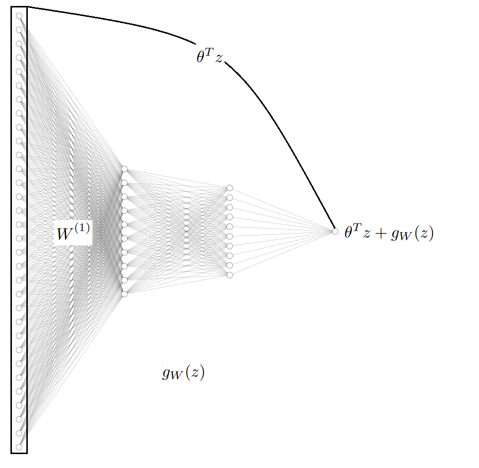
Figure 1: Diagram of the architecture used in the application to NHANES data. The total number of parameters is $p=483$

2.2 Data and estimation

Let $T_{i}$ be the $i$th patient’s unobservable failure time for $i=1,\ldots,n$. In a general interval-censoring scheme, data can be expressed as

$$\left(Z_{i},U_{i},V_{i},\delta_{1i}=1_{\left[T_{i}\leq U_{i}\right]},\delta_{2i}=1_{\left[U_{i}<T_{i}\leq V_{i}\right]}\right),\quad i=1,\ldots,n,$$

where $Z_{i}\in\mathbb{R}^{d}$ is the vector of observed covariates and $U_{i}\leq V_{i}$ are two random checkup time points for individual $i$. Given an i.i.d. sample as above, the parameter-of-interest space is

$$\Gamma=\left\{\left(\Lambda(U_{1}),\dotsc,\Lambda(U_{n}),\Lambda(V_{1}),\ldots,\Lambda(V_{n}),\theta,W\right)\in\mathbb{R}^{n}\times\mathbb{R}^{n}\times\mathbb{R}^{d}\times\mathbb{R}^{N}\right\}$$

where $N$ is the total number of weights involved in the hidden layers of the deep residual block. Now, under (A1) to (A3) as in (Huang and Wellner, 1997), the non-parametric log-likelihood function is

$$l_{n}(\theta,W,\Lambda)= \sum_{i=1}^{n}\left\{\delta_{1i}\log\left[1-\exp\left(-\Lambda\left(U_{i}\right)e^{r_{\theta,W}(Z_{i})}\right)\right]\right.$$

$$+\delta_{2i}\log\left[\exp\left(-\Lambda\left(U_{i}\right)e^{r_{\theta,W}(Z_{i})}\right)-\exp\left(-\Lambda\left(V_{i}\right)e^{r_{\theta,W}(Z_{i})}\right)\right]$$

$$\left.-\delta_{3i}\Lambda\left(V_{i}\right)e^{r_{\theta,W}(Z_{i})}\right\},$$

where $\delta_{3i}=1-\delta_{1i}-\delta_{2i}$. We outline in Algorithm 1 a new optimization routine inspired by the iterative convex minorant (ICM) algorithm (Groeneboom, 1991) and LassoNet’s HIER-PROX (Lemhadri et al., 2021). Essentialy, for each forward pass of $r_{\theta,W}$, we maximize or profile $l_{n}(\theta,W,\Lambda)$ over the nuisance parameter $\Lambda$ (Kosorok, 2008):

$$pl_{n}(\theta,W)=\sup_{\Lambda}l_{n}(\theta,W,\Lambda).$$

The whole optimisation problem is defined therein as

$$\underset{\theta,W}{\operatorname{minimize}}\quad-pl_{n}(\theta,W)+\lambda\|\theta\|_{1}$$

$$\text{ subject to }\left\|W_{j}^{(1)}\right\|_{\infty}\leq M\left|\theta_{j}\right|,j=1,\ldots,d,$$

where $pl_{n}(\theta,W)$ is the profile likelihood obtained with ICM and $W_{j}^{(1)}$ denotes the outward weights for feature $j$ in the first hidden layer. The objective is minimised via the technique of hierarchical proximal optimisation.

Because of the Lasso penalty placed on the objective function, the linear contribution of many input covariates is being shrunk to zero. The constraint imposes that the first hidden layer weights associated with such covariates are also being shrunk to zero. This fact has true regularization implications as the effect of covariates that are screened by the linear Lasso scheme vanishes all the way down forward propagation throughout the hidden layers.

Historically, there are two characterisations of the interval-censored Non-Parameteric Maximum Likelihood Estimator (NPMLE) of the time-to-event distribution function. The first one is owed to (Turnbull, 1976), who attributes it to (Efron, 1967)’s notion of self-consistency. The second one is a perspective based on the theory of isotonic regression that arose in (Groeneboom, 1991). The equations involved in the first case yield to the iteration steps of an expectation-maximization (EM) algorithm whereas the second approach leads to an optimization problem based on ICM which turns out to be much faster than the first one, particularly when working with large sample sizes. We develop an adaptation of the latter that is compatible with deep learning automatic differentiation computational libraries such as torch.autograd, see further details in Appendix A. The high level algorithm is given in Algorithm 1 below.

Algorithm 1

1:Initialize $\theta^{(0)}$, $W^{(0)}$, $\Lambda^{(0)}$, number of epochs $B$, hierarchy multiplier $M$, learning rate $\alpha$, number of iterations $K$

2:Initialize loss function $L^{\left(0\right)}\left(\theta,W\right)$ with $l_{n}\left(\theta,W,\Lambda^{\left(0\right)}\right)$

3:for $k\in\{1\ldots K\}$ do

4:     for $b\in\{1\ldots B\}$ do

5:         Compute gradient of $L^{\left(k\right)}$ w.r.t $\left(\theta,W\right)$ using back-propagation

6:         Update $\theta\leftarrow\theta-\alpha\nabla_{\theta}L$ and $W\leftarrow W-\alpha\nabla_{W}L$

7:         Update $\left(\theta,W_{1}\right)\leftarrow$ HIER-PROX $\left(\theta,W_{1},\alpha\lambda,M\right)$

8:     end for

9:     Run ICM fed with a forward pass of $\theta^{(b)}$ and $W^{(b)}$ to obtain $\Lambda^{\left(k\right)}$

10:     Update loss function $L^{\left(k+1\right)}\left(\theta,W\right)$ with $l_{n}\left(\theta,W,\Lambda^{\left(k\right)}\right)$

11:end for

3 Simulation studies

Times-to-event and censoring indicators were generated as in (Kiani and Arasan, 2012) from the cumulative hazards $\Lambda_{1}(t\mid z)=\Lambda(t)e^{m_{1}(z)}$ and $\Lambda_{2}(t\mid z)=\Lambda(t)e^{m_{2}(z)}$. The chosen baseline survival function is the Gompertz distribution in all cases with $\gamma=5$, $\lambda=1$.

Each simulation consists of two datasets, each generated according to $m_{1}$ and $m_{2}$. The functions $m_{1}$ and $m_{2}$ are defined as follows:

• $m_{1}(z_{1},\ldots,z_{100})=-2z_{1}+5z_{2}+3z_{3}-3z_{4}$

• $m_{1}(z_{1},\ldots,z_{100})=-2z_{1}+5z_{2}+3z_{3}-3z_{4}+2|z_{1}^{3}-3\sin(\pi z_{1})|+4(z_{1}^{2}z_{3}-|z_{2}|)$

The quantities in Tables 1 and 2 represent averages across $1000$ simulation runs. In each simulation, a regularization path from dense to sparse was run according to the warm starts strategy used in (Lemhadri et al., 2021). Essentially, 20 % of the sample was kept away from training and used to compute Integrated Brier Score (IBS) for each $\lambda$ defining the path. Given the test sample $\{\left(Z_{i},U_{i},V_{i},\delta_{1i},\delta_{2i}\right),\quad i\in{\text{random }20\%\text{ of the sample}}\}$ and its correspondent estimates of the conditional survival function $\{\hat{S}\left(t\mid{Z}_{i}\right),\quad i\in{\text{random }20\%\text{ of the sample}}\}$, the time-dependent Brier score is defined as Graf et al. (1999)

$$\mathrm{BS}^{c}(t)=\frac{1}{n}\sum_{i=1}^{n}I\left(Y_{i}\leq t\wedge\gamma_{i}=1\right)\frac{\left(\hat{S}\left(t\mid{Z}_{i}\right)\right)^{2}}{\hat{G}\left(Y_{i}\right)}+I\left(Y_{i}>t\right)\frac{\left(1-\hat{S}\left(t\mid Z_{i}\right)\right)^{2}}{\hat{G}(t)}$$

where $\gamma_{i}=1-\delta_{3i}$, $Y_{i}=\frac{U_{i}+V_{i}}{2}$ and $\hat{G}(\cdot)$ is the estimated probability of the event $\{\gamma_{i}=0\}$ using the training sample. Given this, the Integrated Brier Score between two pre-defined time instants $t_{1}$ and $t_{2}$ is defined as $\operatorname{IBS}=\int_{t_{1}}^{t_{2}}\frac{t\mathrm{BS}^{c}(t)}{t_{2}}dt$. For our study, we chose $t_{1}$ and $t_{2}$ to be the 0.05 and the 0.95 empirical quantiles of the merged interval borders.

Within a simulation run, the chosen model is the minimizer of IBS. Therefore, using the best models picked in each run, we computed four averaged metrics that are collected in Tables 1 and 2.

In Table 1, we compare Interval Censored Recursive Forests (Cho et al., 2021) and our approach across several sample sizes with IBS and the estimation error in $\ell_{2}$ norm of the cumulative hazard baseline function (it is possible to compute it because we know the ground time distribution).

In Table 2 we restrict ourselves to analyse the empirical behavior of our approach using three different metrics. In all cases, the covariates were simulated according to a multivariate normal with correlation between covariate $i$ and $j$ given by $0.5^{|i-j|}$

The main conclusions that can be extracted from Tables 1 and 2 are the following. First, the performance of our approach is empirically superior to Interval Censored Survival Forests in terms of both IBS score and approximation error of the baseline cumulative hazard function. Second, focusing attention in our proposal, performance increases when increasing sample size according to all the metrics.

Table 1: Performance comparison of Interval Censored Recursive Forests (Cho et al., 2021) with our approach accross different metrics and sample sizes.

		ICRF			Our approach
		$n=500$	$n=1000$	$n=2000$	$n=500$	$n=1000$	$n=2000$
IBS	$m_{1}$	0.266	0.262	0.261	0.181	0.180	0.179
	$m_{2}$	0.227	0.217	0.208	0.219	0.218	0.217
$\|\hat{\Lambda}-{\Lambda}\|_{L^{2}}$	$m_{1}$	1.18	1.10	1.01	0.31	0.21	0.17
	$m_{2}$	7.94	7.05	6.81	0.20	0.12	0.10

Table 2: Performance check of exclusively our approach across three additional metrics and different sample sizes.

		Our approach
		$n=500$	$n=1000$	$n=2000$
$R^{2}(r_{\hat{\theta},\hat{W}},m_{i})$	$m_{1}$	0.975	0.978	0.985
	$m_{2}$	0.744	0.821	0.904
% of TP	$m_{1}$	0.89	0.92	0.95
	$m_{2}$	0.67	0.81	0.88
% of TN	$m_{1}$	0.92	0.93	0.94
	$m_{2}$	0.89	0.90	0.90

4 Application to the NHANES 2003-2006 wave cycle

The National Health and Nutrition Examination Survey (NHANES) is an extensive major program conducted by the National Center for Health Statistics (NCHS), one of the Centers for Disease Control (CDC), that collects health and nutrition data from the U.S. population.

Their main objective is to monitor the lifestyle of the U.S. population over time, for example, to determine the prevalence of risk factors in a broad spectrum of diseases such as Diabetes Mellitus.

The NHANES data are publicly available from the CDC (https://www.cdc.gov/nchs/nhanes/index.htm) and are broadly categorized into six areas: demographics, dietary, examination, laboratory, questionnaires, and limited access. The registered variables consist of phenotype and environmental exposure information on each individual. The accelerometer data for a particular NHANES cohort can be downloaded from the "Physical Activity Monitor" subcategory under the "Examination data" tab. In this work, a subset of $n=1525$ patients that are between $65$ and $85$ years old will be used.

The primary purpose of our analysis is to evaluate the effectiveness of our new non-linear regression feature selection algorithm and compare it with the traditional Cox model. For this purpose, we randomly split the sample into a training set (80 % of the total) and a test set (the remaining 20 %) and fit both models with the variables listed in Table 3. Table 3 also collects the variables selected by our model and Figure 2 displays metrics quantifying the performance of our proposal in comparison with the traditional Cox model. Although advantages are important, we believe that the prediction accuracy of our algorithm could be improved with more participants.

To display in a more easy format some actual results drawn by our model, Figure 3 shows survival curves predicted by our model for the variable Gender, Age, CHF and TAC. In addition, we show in Figure 4 the interaction of TAC with the age, stratified by gender. A first sight conclusion from Figure 4 is that males that have exercised the least are at twice as much risk compared to those who have exercised the most when they reach 70 years old. Also, a clear difference in the cumulative risk between males and females can be noted there. Notably, the daily energy expenditure is high, and the risk decreases significantly near middle-aged, elderly individuals. For example, high values for the TAC variable can reduce the hazard ratio by more than one point.

We select the TAC for this graphical analysis because it has been reported by several studies to be the most effective physical activity summary variable across different databases, such as UK biobank and NHANES.

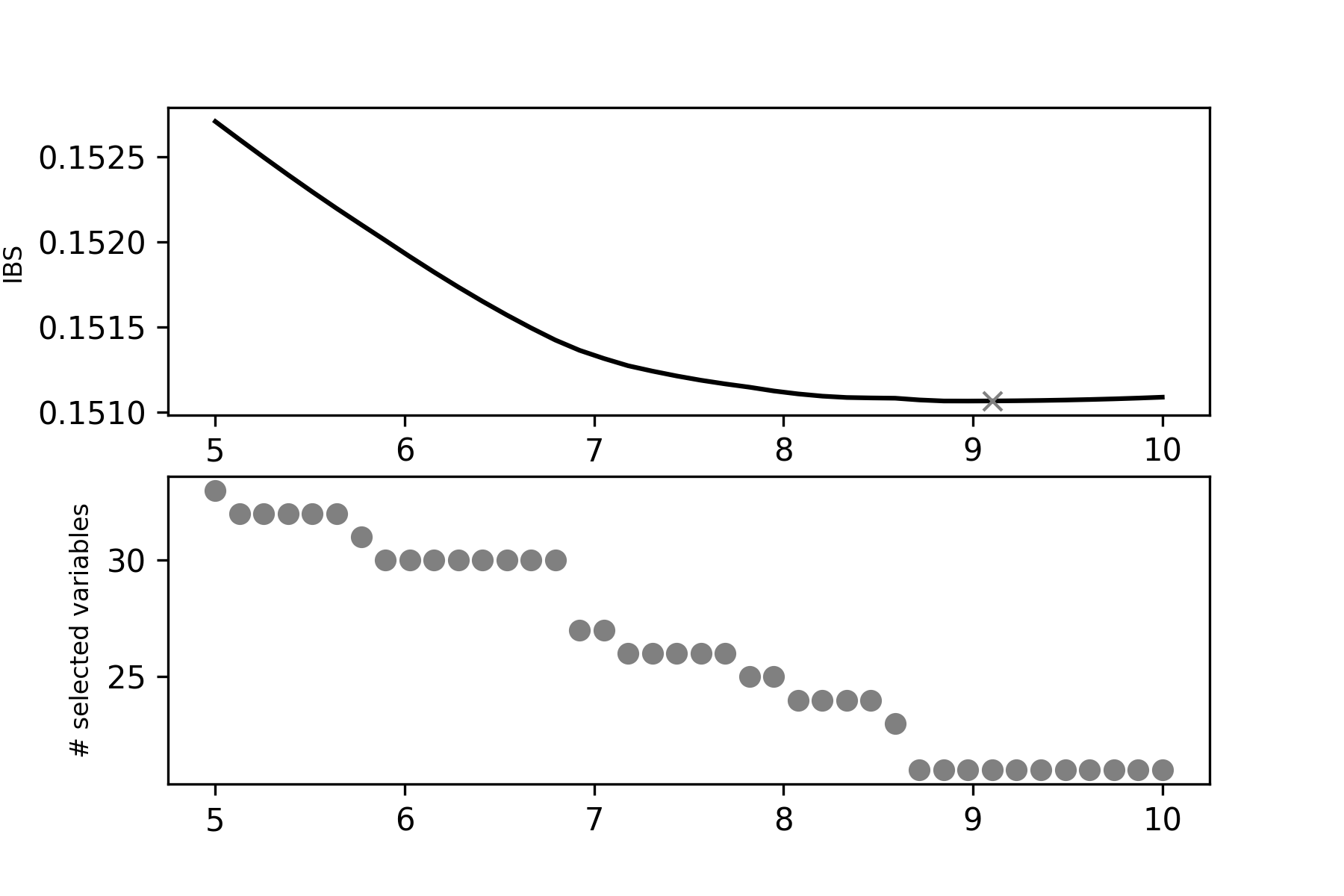
Figure 2: Integrated Brier Score (IBS) of the traditional Cox model was 0.24 and 0.17 for Interval Censored Recursive Forests. Using the optimal $\lambda$ across the warm starts regularization path, we see that our model achieves 0.15 IBS, which is 33 % less.

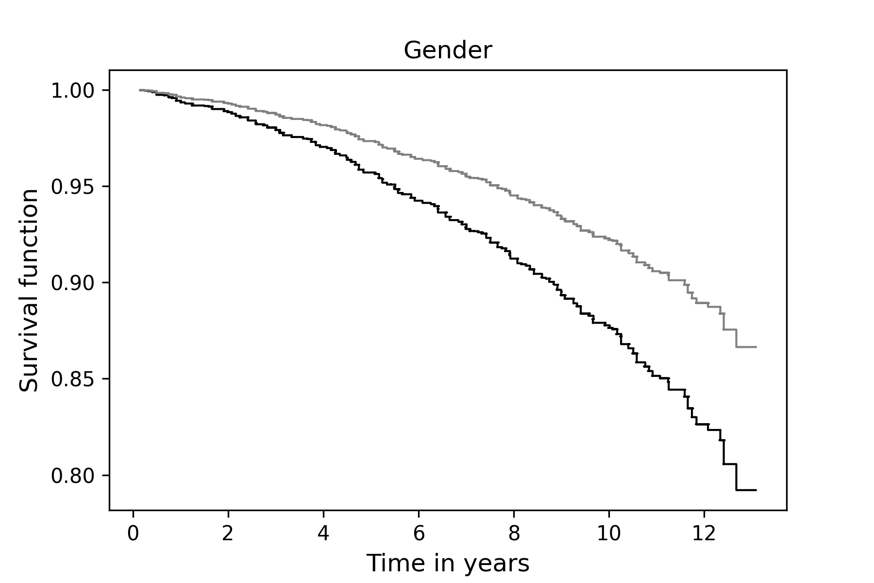
(a)

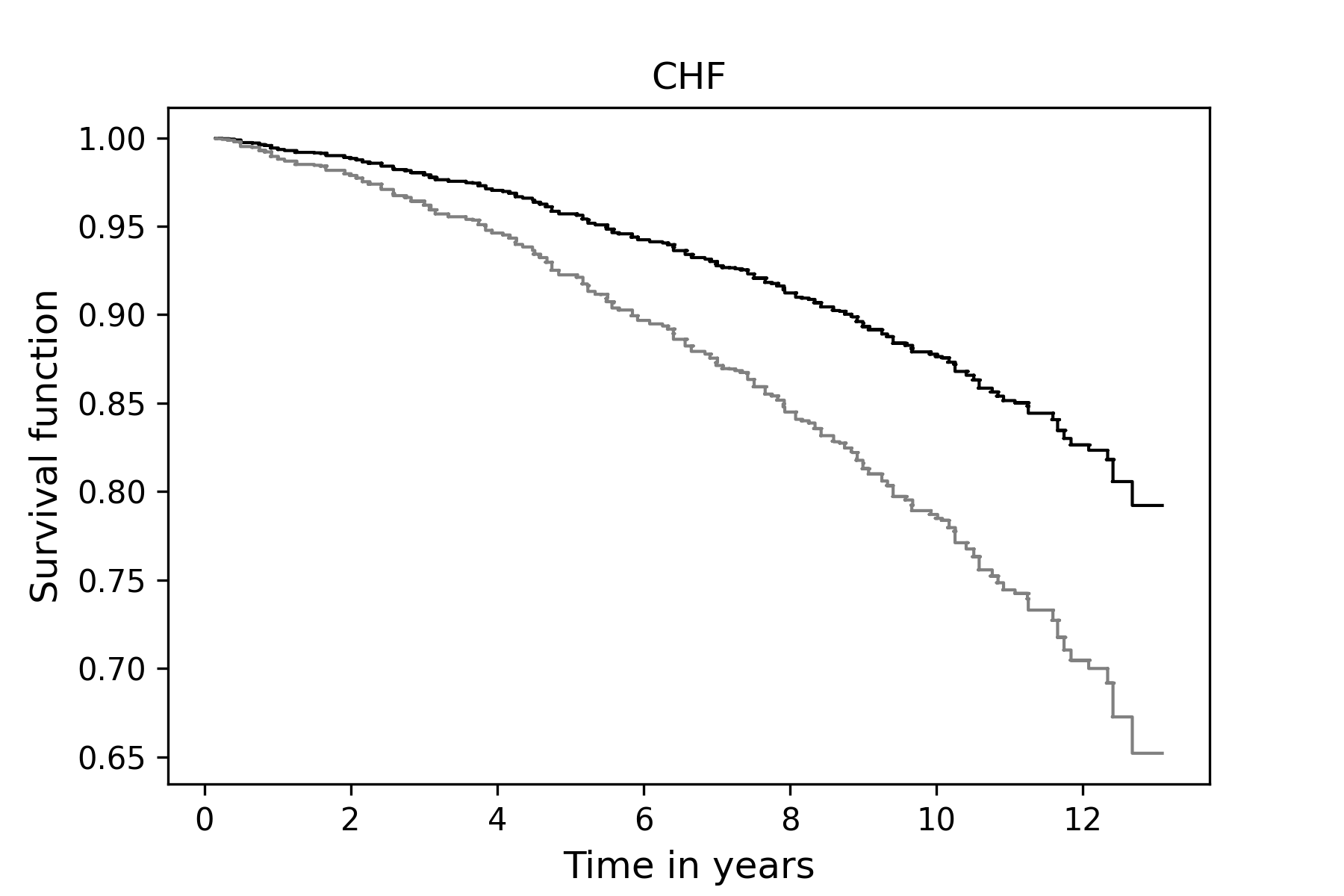
(b)

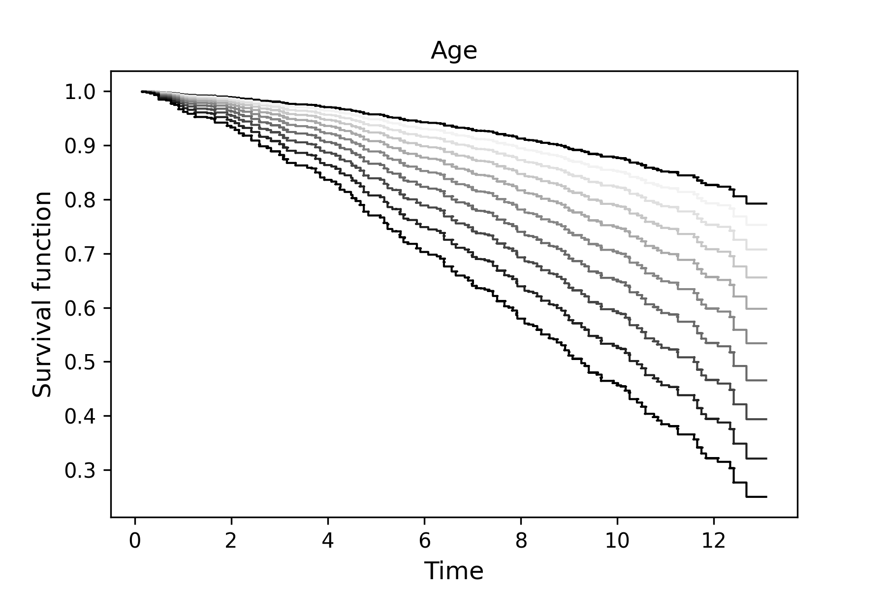
(c)

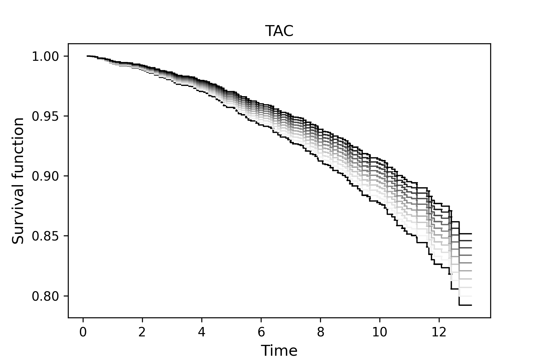
(d)

Figure 3: Estimated survival functions for several configurations of the covariates. Note that the black graph, the baseline survival function, is the same across all the plots. In (c), the different curves were estimated by doing forward passes of different ages through our model keeping the rest of the variables at zero. More intense greens correspond to higher ages, and the darkest green corresponds to the age of the oldest person in the dataset. The same idea holds for (d), but varying TAC and setting the rest of the covariates to zero. In (a), green stands for female and black for male. In (b), green stands for suffering congestive heart failure and black stands for the opposite. First hints of non-linearity can be perceived in that the grid of different TAC values on which predictions were launched was equally-spaced, whereas the resulting predicted survival curves are not.

Table 3: Variable summaries in the NHANES data. In the last two columns we respectively show the coefficients of the linear part in the neural model and the coefficients estimated with the traditional Cox model.

. Variable NHANES code Description Support Selected $\hat{\theta}$ $\hat{\theta}_{Cox}$ $X_{1}$ Gender 0: Male, 1: Female Yes -0.4855 -0.5960 $X_{2}$ Cancer 0: No, 1: Yes No 0 0.0034 $X_{3}$ Stroke 0: No, 1: Yes No 0.1644 0.2758 $X_{4}$ Diabetes 0: No, 1: Yes Yes 0.1528 0.2645 $X_{5}$ BMI 0: Normal, 1: Overweight No 0 0.0210 $X_{6}$ CHF Congesive Heart Failure 0: No, 1: Yes Yes 0.6072 0.7187 $X_{7}$ CHD Coronary Heart Disease 0: No, 1: Yes Yes 0 0.0988 $X_{8}$ Mobility Problem 0: No, 1: Yes No 0.2673 0.3793 $X_{9}$ RIDAGEYR Age at the interview time Continuous Yes 1.7821 1.8942 $X_{10}$ LBXTC Total Cholesterol Continuous Yes 0 0.0988 $X_{11}$ LBDHDD Direct HDL-Cholesterol Continuous Yes 0.2380 0.3497 $X_{12}$ SYS Systolic Blood Pressure Continuous No 0.4362 0.5481 $X_{13}$ TAC Total volume of physical activity Continuous No -0.3725 -0.4835 $X_{14}$ TLAC Total log activity counts Continuous No 0 -0.095 $X_{15}$ WT Accelerometer wear time Continuous Yes 0.0306 0.1425 $X_{16}$ ST sedentary Time Continuous No 0.5481 0.048 $X_{17}$ MVPA Moderate-to-Vigorous Physical Activity Continuous Yes -0.2649 -0.3761 $X_{18}$ ABout Continuous Yes -0.1545 -0.2654 $X_{19}$ SBout Continuous No 0 0.0805 $X_{20}$ SATP Sedentary-to-active transition prob. Continuous Yes 0.1776 0.2896 $X_{21}$ ASTP Active-to-sedentary transition prob. Continuous Yes 0.9963 1.1082 $X_{22}$ $\texttt{TLAC}_{1}$ Total log activity counts 12AM-2AM Continuous No 0 -0.018 $X_{23}$ $\texttt{TLAC}_{2}$ Total log activity counts 2AM-4PM Continuous Yes 0.2150 0.3264 $X_{24}$ $\texttt{TLAC}_{3}$ Total log activity counts 4PM-6PM Continuous Yes 0.1001 0.2115 $X_{25}$ $\texttt{TLAC}_{4}$ Total log activity counts 6PM-8PM Continuous Yes -0.1048 -0.2157 $X_{26}$ $\texttt{TLAC}_{5}$ Total log activity counts 8PM-10PM Continuous No 0 0.0544 $X_{27}$ $\texttt{TLAC}_{6}$ Total log activity counts 10PM-12PM Continuous Yes -0.3908 -0.5012 $X_{28}$ $\texttt{TLAC}_{7}$ Total log activity counts 12PM-2AM Continuous Yes 0.0853 0.1975 $X_{29}$ $\texttt{TLAC}_{8}$ Total log activity counts 2AM-4AM Continuous No 0 -0.0722 $X_{30}$ $\texttt{TLAC}_{9}$ Total log activity counts 4AM-6AM Continuous No 0 -0.0990 $X_{31}$ $\texttt{TLAC}_{10}$ Total log activity counts 4AM-6AM Continuous No 0 0.0447 $X_{32}$ $\texttt{TLAC}_{11}$ Total log activity counts 6AM-8AM Continuous Yes -0.2322 -0.3430 $X_{33}$ $\texttt{TLAC}_{12}$ Total log activity counts 8AM-10AM Continuous Yes -0.1529 -0.2640

(a) Estimated hazard ratio for males

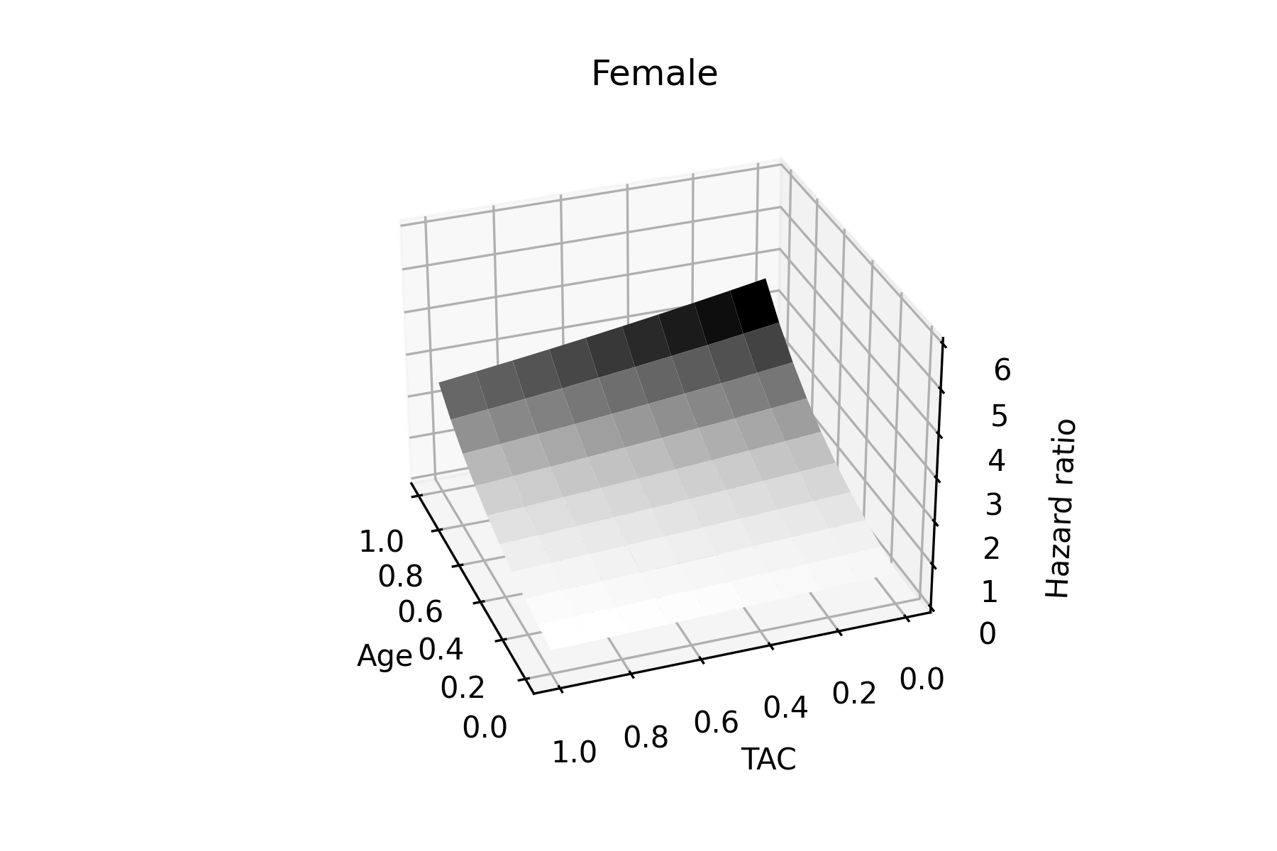
(b) Estimated hazard ratio for females

Figure 4: Neural hazard ratio fixing all the covariates but TAC and age. Minimum and maximum ages, encoded in the plot as 0 and 1 respectively, are 65 and 85 years old. For both sexes, even though becoming older exposure risk to death can be considerably reduced by doing enough exercise. This figure pictures the idea that deep learning is able to intrinsically express model-free interactions. The hazard function as a function of these two variables is already highly non-linear per se, and when a third variable comes into play as age we see that the regression surface is not modified by a simple shift. For male, it is harder to reduce the mortality risk at elderly by exercising.

5 Discussion

The main contribution of this paper is to propose a new neural lasso Cox regression algorithm for interval-censored outcomes without assuming any functional form for the Cox model parametric component. At the same time, we select the most relevant features simultaneously. To the best of our knowledge, this is the first methodological contribution in interval-censored data and one of the first in the context of incomplete information that combines semi-parametric statistical models with deep learning algorithms.

Significant recent progress appeared in this field with the development of new random forest models Cho et al. (2021); Yao et al. (2019) that overcome many limitations of the traditional Cox model and accelerated failure risk model to fight against strongly non-linear functional dependencies between survival times and covariates. However, as we can see in the simulations, when the signal is sparse, the performance of the random survival forest is weaker than our proposal. Importantly, we assume in this synthetic example that non-linear Cox models are behind data generation. This could be considered to be a strong assumption in many applications. A potential improvement of our proposal to avoid this limitation is introducing a new deep lasso time-dependent Cox model Bacchetti and Quale (2002). In addition, a more particular neural network architecture that captures better the expressivity of biomarkers can be created. However, our current approach is already easily interpretable in terms of the effect and interaction of covariates.

Some new exciting research directions arise from the work proposed here, including the development of interval-censored models that face causal problems. However, due to the difficulties of causal interpretations of Cox models Martinussen (2022), it had better be pursued from the perspective of the accelerated failure times model. Another critical challenge is providing a measure of uncertainty of new predictions, particularly in medical science applications, due to a sizeable inherent uncertainty of patient evolution. In this direction, the extension of conformal inference ideas can be a promising direction to address these scientific challenges thanks to the existence of likelihood equations in our model; we can use existing approaches of right-censored data Teng et al. (2021) and split-conformal Izbicki et al. (2022). Finally, another primary research direction is establishing the significance of each selected variable, the first post-selection methodology for neural models has recently appeared (see for example Zhu et al. (2021)).

References

- Huang [1996] Jian Huang. Efficient estimation for the proportional hazards model with interval censoring. The Annals of Statistics, 24(2):540 – 568, 1996. doi:10.1214/aos/1032894452. URL https://doi.org/10.1214/aos/1032894452.
- Wu and Cook [2020] Ying Wu and Richard J Cook. Assessing the accuracy of predictive models with interval-censored data. Biostatistics, 23(1):18–33, 03 2020. ISSN 1465-4644. doi:10.1093/biostatistics/kxaa011. URL https://doi.org/10.1093/biostatistics/kxaa011.
- Cho et al. [2021] Hunyong Cho, Nicholas P. Jewell, and Michael R. Kosorok. Interval censored recursive forests. Journal of Computational and Graphical Statistics, 0(0):1–13, 2021. doi:10.1080/10618600.2021.1987253. URL https://doi.org/10.1080/10618600.2021.1987253.
- Yao et al. [2019] Weichi Yao, Halina Frydman, and Jeffrey S Simonoff. An ensemble method for interval-censored time-to-event data. Biostatistics, 22(1):198–213, 07 2019. ISSN 1465-4644. doi:10.1093/biostatistics/kxz025. URL https://doi.org/10.1093/biostatistics/kxz025.
- Travis-Lumer and Goldberg [2021] Yael Travis-Lumer and Yair Goldberg. Kernel machines for current status data. Machine Learning, 110(2):349–391, 2021.
- Rindt et al. [2022] David Rindt, Robert Hu, David Steinsaltz, and Dino Sejdinovic. Survival regression with proper scoring rules and monotonic neural networks. In International Conference on Artificial Intelligence and Statistics, pages 1190–1205. PMLR, 2022.
- Zhong et al. [2021] Qixian Zhong, Jonas W Mueller, and Jane-Ling Wang. Deep extended hazard models for survival analysis. Advances in Neural Information Processing Systems, 34, 2021.
- Lee et al. [2018] Changhee Lee, William Zame, Jinsung Yoon, and Mihaela Van Der Schaar. Deephit: A deep learning approach to survival analysis with competing risks. In Proceedings of the AAAI conference on artificial intelligence, volume 32, 2018.
- Steingrimsson and Morrison [2020] Jon Arni Steingrimsson and Samantha Morrison. Deep learning for survival outcomes. Statistics in medicine, 39(17):2339–2349, 2020.
- Jia and Jeong [2022] Yichen Jia and Jong-Hyeon Jeong. Deep learning for quantile regression under right censoring: Deepquantreg. Computational Statistics & Data Analysis, 165:107323, 2022.
- Gao et al. [2019] F. Gao, D. Zeng, D. Couper, and D. Y. Lin. Semiparametric Regression Analysis of Multiple Right- and Interval-Censored Events. J Am Stat Assoc, 114(527):1232–1240, 2019.
- Li et al. [2020] Chenxi Li, Daewoo Pak, and David Todem. Adaptive lasso for the Cox regression with interval censored and possibly left truncated data. Statistical Methods in Medical Research, 29(4):1243–1255, 2020. doi:10.1177/0962280219856238. URL https://doi.org/10.1177/0962280219856238. PMID: 31203741.
- Tibshirani [1996] Robert Tibshirani. Regression shrinkage and selection via the lasso. Journal of the Royal Statistical Society: Series B (Methodological), 58(1):267–288, 1996. doi:https://doi.org/10.1111/j.2517-6161.1996.tb02080.x. URL https://rss.onlinelibrary.wiley.com/doi/abs/10.1111/j.2517-6161.1996.tb02080.x.
- Tibshirani [1997] Robert Tibshirani. The lasso method for variable selection in the cox model. Statistics in Medicine, 16(4):385–395, 1997. doi:https://doi.org/10.1002/(SICI)1097-0258(19970228)16:4<385::AID-SIM380>3.0.CO;2-3. URL https://onlinelibrary.wiley.com/doi/abs/10.1002/%28SICI%291097-0258%2819970228%2916%3A4%3C385%3A%3AAID-SIM380%3E3.0.CO%3B2-3.
- van de Geer, [1993] van de Geer, S. (1993). Hellinger-Consistency of Certain Nonparametric Maximum Likelihood Estimators. The Annals of Statistics, 21(1):14 – 44.
- Bühlmann and Van De Geer, [2011] Bühlmann, P. and Van De Geer, S. (2011). Statistics for high-dimensional data: methods, theory and applications. Springer Science & Business Media.
- Bertsimas et al. [2020] Dimitris Bertsimas, Jean Pauphilet, and Bart Van Parys. Sparse regression: Scalable algorithms and empirical performance. Statistical Science, 35(4):555–578, 2020.
- Freijeiro-González et al. [2022] Laura Freijeiro-González, Manuel Febrero-Bande, and Wenceslao González-Manteiga. A critical review of lasso and its derivatives for variable selection under dependence among covariates. International Statistical Review, 90(1):118–145, 2022. doi:https://doi.org/10.1111/insr.12469. URL https://onlinelibrary.wiley.com/doi/abs/10.1111/insr.12469.
- Bertsimas et al. [2016] Dimitris Bertsimas, Angela King, and Rahul Mazumder. Best subset selection via a modern optimization lens. The annals of statistics, 44(2):813–852, 2016.
- Hazimeh and Mazumder [2020] Hussein Hazimeh and Rahul Mazumder. Fast best subset selection: Coordinate descent and local combinatorial optimization algorithms. Operations Research, 68(5):1517–1537, 2020.
- Huang et al. [2010] Jian Huang, Joel L Horowitz, and Fengrong Wei. Variable selection in nonparametric additive models. Annals of statistics, 38(4):2282, 2010.
- Lemhadri et al. [2021] Ismael Lemhadri, Feng Ruan, and Rob Tibshirani. Lassonet: Neural networks with feature sparsity. In Arindam Banerjee and Kenji Fukumizu, editors, Proceedings of The 24th International Conference on Artificial Intelligence and Statistics, volume 130 of Proceedings of Machine Learning Research, pages 10–18. PMLR, 13–15 Apr 2021. URL https://proceedings.mlr.press/v130/lemhadri21a.html.
- McGregor et al. [2020] DE McGregor, J Palarea-Albaladejo, PM Dall, K Hron, and SFM Chastin. Cox regression survival analysis with compositional covariates: application to modelling mortality risk from 24-h physical activity patterns. Statistical methods in medical research, 29(5):1447–1465, 2020.
- Smirnova et al. [2020] Ekaterina Smirnova, Andrew Leroux, Quy Cao, Lucia Tabacu, Vadim Zipunnikov, Ciprian Crainiceanu, and Jacek K Urbanek. The predictive performance of objective measures of physical activity derived from accelerometry data for 5-year all-cause mortality in older adults: National health and nutritional examination survey 2003–2006. The Journals of Gerontology: Series A, 75(9):1779–1785, 2020.
- Cox [1972] D. R. Cox. Regression models and life-tables. Journal of the Royal Statistical Society: Series B (Methodological), 34(2):187–202, 1972. doi:https://doi.org/10.1111/j.2517-6161.1972.tb00899.x. URL https://rss.onlinelibrary.wiley.com/doi/abs/10.1111/j.2517-6161.1972.tb00899.x.
- Lin and Jegelka [2018] Hongzhou Lin and Stefanie Jegelka. Resnet with one-neuron hidden layers is a universal approximator. In S. Bengio, H. Wallach, H. Larochelle, K. Grauman, N. Cesa-Bianchi, and R. Garnett, editors, Advances in Neural Information Processing Systems, volume 31. Curran Associates, Inc., 2018. URL https://proceedings.neurips.cc/paper/2018/file/03bfc1d4783966c69cc6aef8247e0103-Paper.pdf.
- Huang and Wellner [1997] Jian Huang and Jon A. Wellner. Interval censored survival data: A review of recent progress. Proceedings of the First Seattle Symposium in Biostatistics: Survival Analysis, Lecture Notes in Statistics, 123, 1997.
- Groeneboom [1991] Piet Groeneboom. Nonparametric maximum likelihood estimators for interval censoring and deconvolution. Technical report 378, Stanford University, 1991.
- Kosorok [2008] Michael R. Kosorok. Introduction to Empirical Processes and Semiparametric Inference. Springer New York, 2008. doi:10.1007/978-0-387-74978-5. URL http://dx.doi.org/10.1007/978-0-387-74978-5.
- Turnbull [1976] Bruce W Turnbull. The empirical distribution function with arbitrarily grouped, censored and truncated data. Journal of the Royal Statistical Society: Series B (Methodological), 38(3):290–295, 1976.
- Efron [1967] Bradley Efron. The two sample problem with censored data. In Proceedings of the fifth Berkeley symposium on mathematical statistics and probability, pages 831–853, 1967.
- Kiani and Arasan [2012] Kaveh Kiani and Jayanthi Arasan. Simulation of interval censored data in medical and biological studies. International Journal of Modern Physics: Conference Series, 09:112–118, 2012. doi:10.1142/S2010194512005168. URL https://doi.org/10.1142/S2010194512005168.
- Graf et al. [1999] E. Graf, C. Schmoor, W. Sauerbrei, and M. Schumacher. Assessment and comparison of prognostic classification schemes for survival data. Stat Med, 18(17-18):2529–2545, 1999.
- Bacchetti and Quale [2002] Peter Bacchetti and Christopher Quale. Generalized additive models with interval-censored data and time-varying covariates: Application to human immunodeficiency virus infection in hemophiliacs. Biometrics, 58(2):443–447, 2002.
- Martinussen [2022] Torben Martinussen. Causality and the cox regression model. Annual Review of Statistics and Its Application, 9, 2022.
- Teng et al. [2021] Jiaye Teng, Zeren Tan, and Yang Yuan. T-sci: A two-stage conformal inference algorithm with guaranteed coverage for cox-mlp. In International Conference on Machine Learning, pages 10203–10213. PMLR, 2021.
- Izbicki et al. [2022] Rafael Izbicki, Gilson Shimizu, and Rafael B Stern. Cd-split and hpd-split. Journal of Machine Learning Research, 23:1–32, 2022.
- Zhu et al. [2021] Zifan Zhu, Yingying Fan, Yinfei Kong, Jinchi Lv, and Fengzhu Sun. Deeplink: Deep learning inference using knockoffs with applications to genomics. Proceedings of the National Academy of Sciences, 118(36), 2021.