Influence of impurities on electronic structure in cuprate superconductors

Abstract

The impurity is inherently manifest in cuprate superconductors, as cation substitution or intercalation is necessary for the introduction of charge carriers, and its influence on the electronic state is at the heart of a great debate in physics. Here based on the microscopic octet scattering model, the influence of the impurity scattering on the electronic structure of cuprate superconductors is investigated in terms of the self-consistent $T$-matrix approach. The impurity scattering self-energy is evaluated firstly in the Fermi-arc-tip approximation of the quasiparticle excitations and scattering processes, and the obtained results show that the decisive role played by the impurity scattering self-energy in the particle-hole channel is the further renormalization of the quasiparticle band structure with a reduced quasiparticle lifetime, while the impurity scattering self-energy in the particle-particle channel induces a strong deviation from the d-wave behaviour of the superconducting gap, leading to the existence of a finite gap over the entire electron Fermi surface. Moreover, these impurity scattering self-energies are employed to study the exotic features of the line-shape in the quasiparticle excitation spectrum and the autocorrelation of the quasiparticle excitation spectra, and the obtained results are then compared with the corresponding experimental data. The theory therefore also indicates that the unconventional features of the electronic structure in cuprate superconductors is generated by both the strong electron correlation and impurity scattering.

I INTRODUCTION

The single common feature in the crystal structure of cuprate superconductors is the presence of the square-lattice CuO₂ layer Bednorz86 ; Wu87 , which are believed to contain all the essential physics. The layered crystal structure then is a stacking of CuO₂ layers separated by other oxide layers, which maintain the charge neutrality and cohesion of the structure mainly through ionic interactions Bednorz86 ; Wu87 . The parent compound of cuprate superconductors is a Mott insulator with an antiferromagnetic (AF) long-range order Fujita12 , and superconductivity then is realized when this AF long-range order state is suppressed by doped charge carriers into the CuO₂ layer Bednorz86 ; Wu87 . In addition to the change of the charge-carrier concentration, this doping process nearly always introduces some measure of disorder Hussey02 ; Balatsky06 ; Alloul09 , leading to that in principle, all cuprate superconductors have naturally impurities (or disorder). In particular, impurities which substitute for Cu in the CuO₂ layer turn out to be strong scatters of the electronic state in the layer Hussey02 ; Balatsky06 ; Alloul09 . The importance of the understanding of the influence of the impurity scattering on the electronic structure has been quickly recognized, since many of the unconventional features, including the relatively high superconducting (SC) transition temperature $T_{\rm c}$, have often been attributed to particular characteristics of the low-energy quasiparticle excitations determined by the electronic structure Damascelli03 ; Campuzano04 ; Fink07 .

The impurity scattering in cuprate superconductors is specially unconventional, and manifests a variety of the phenomena depending on the strength of the electron correlation, charge-carrier doping, temperature, and magnetic field Hussey02 ; Balatsky06 ; Alloul09 . Experimentally, by virtue of systematic studies using multiple measurement techniques, a number of consequences from the impurity scattering together with the associated fluctuation phenomena have been identified Hussey02 ; Balatsky06 ; Alloul09 , where an agreement has emerged that the various properties of the d-wave SC-state in the pure system are extreme sensitivity to the influence of the impurity scattering than that in the conventional superconductors. This follows a basic fact that the influence of the impurity scattering on the d-wave SC-state is to break the electron pairs and to mix the SC gap with different signs on different parts of the electron Fermi surface (EFS) Hussey02 ; Balatsky06 ; Alloul09 . In particular, the early experimental measurements Ishida91 ; Legris93 ; Giapintzakis94 ; Fukuzumi96 ; Attfield98 ; Bobroff99 ; Eisaki04 showed that the influence of the impurity scattering tends to suppress the SC coherence, and then $T_{\rm c}$ is found to be depressed rapidly with the increase of the impurity concentration. Later, the experimental observations indicated that the extent of the deviation from the d-wave SC gap form increases with the increase of the impurity concentration Vobornik99 ; Vobornik00 ; Shen04 ; Kondo07 ; Pan09 . This impurity concentration dependence of the suppression of $T_{\rm c}$ thus has been reflected in the nature of the SC-state quasiparticle excitations resulting of the dressing of the electrons via the impurity scattering, where a change from linear temperature dependence to the quadratic behavior in the magnetic-field penetration-depth occurs due to the influence of the impurity scattering Bonn94 , while the ratio of the low-temperature superfluid density and the effective mass of the electrons $n_{\rm s}(T\rightarrow 0)/m^{*}$ is observed experimentally to decrease with the increase of the impurity concentration Bucci94 ; Bernhard96 ; Bobroff05 . In particular, the angle-resolved photoemission spectroscopy (ARPES) experiments Vobornik99 ; Vobornik00 ; Shen04 ; Kondo07 ; Pan09 indicate that the spectral linewidth of the quasiparticle excitation spectrum broadens rapidly with the increase of the impurity concentration, leading to that the spectral intensity is suppressed almost linearly in energy at low temperatures. These experimental results therefore offer experimental evidences that the electronic structure and SC-state properties in the pure cuprate superconductors are significantly influenced by the impurity scattering.

Although a number of consequences from the impurity scattering Hussey02 ; Balatsky06 ; Alloul09 together with the associated fluctuation phenomena have been well-identified experimentally Vobornik99 ; Vobornik00 ; Shen04 ; Kondo07 ; Pan09 ; Bonn94 ; Bucci94 ; Bernhard96 ; Bobroff05 , the full understanding of the influence of the impurity scattering on the electronic state is still a challenging issue. Theoretically, the homogenous part of the SC-state electron propagator in the preceding discussions is based on the modified Bardeen-Cooper-Schrieffer (BCS) formalism with the d-wave symmetry Hussey02 ; Balatsky06 ; Alloul09 , and then the coupling between the electrons and impurities as the perturbation is treated in terms of the self-consistent T-matrix approach for a single impurity or a finite impurity concentration Hussey02 ; Balatsky06 ; Alloul09 ; Mahan81 ; Hirschfeld89 ; Hirschfeld93 . In particular, the characteristic feature of the d-wave SC-state is the existence of four nodes on EFS, where the SC gap vanishes, and then the SC-state properties are largely governed by the quasiparticle excitations at around the nodal region Hussey02 ; Balatsky06 ; Alloul09 . In this case, the impurity scattering self-energy was evaluated in the nodal approximation of the quasiparticle excitations and scattering processes Hussey02 ; Balatsky06 ; Alloul09 , and was used to discuss the various properties of the SC-state in cuprate superconductors Hussey02 ; Balatsky06 ; Alloul09 ; Durst00 ; Yashenkin01 ; Nunner05 ; Dahm05 ; Wang08 ; Andersen08 ; Wang09 ; Hone17 . However, it has been demonstrated experimentally Chatterjee06 ; He14 that the Fermi arcs formed by the disconnected segments on the constant energy contour that emerge due to the EFS reconstruction at the case of zero energy Shi08 ; Sassa11 ; Comin14 ; Horio16 ; Loret18 can persist into the case for a finite binding-energy, where the quasiparticle scattering further reduces almost all spectral weight on Fermi arcs to the tips of the Fermi arcs, and then the most physical properties are mainly controlled by the quasiparticle excitations at around the tips of the Fermi arcs. Moreover, these tips of the Fermi arcs connected by the scattering wave vectors ${\bf q}_{i}$ construct a octet scattering model, and then the quasiparticle scattering processes with the scattering wave vectors ${\bf q}_{i}$ contribute effectively to the quasiparticle scattering processes Chatterjee06 ; He14 . It should be emphasized that this octet scattering model is a basic model in the explanation of the Fourier transform scanning tunneling spectroscopy experimental data Yin21 ; Pan01 ; Hoffman02 ; Kohsaka07 ; Kohsaka08 ; Hamidian16 , and also can give a consistent description of the regions of the highest joint density of states detected from the ARPES autocorrelation experiments Chatterjee06 ; He14 . However, to the best of our knowledge, the influence of the impurity scattering on the electronic structure has not been discussed starting from the microscopic octet scattering model to treat the impurity scattering in terms of the self-consistent $T$-matrix approach, and no explicit calculation of the impurity scattering self-energy has been made so far in the Fermi-arc-tip approximation of the quasiparticle excitations and scattering processes.

In this paper, we start from the homogenous part of the electron propagator and the related microscopic octet scattering model obtained within the framework of the kinetic-energy-driven superconductivity Feng0306 ; Feng12 ; Feng15a ; Feng15 to study the influence of the impurity scattering on the electronic structure of cuprate superconductors in terms of the self-consistent $T$-matrix approach, where we evaluate firstly the impurity scattering self-energy in the Fermi-arc-tip approximation of the quasiparticle excitations and scattering processes, and the obtained results show that (i) the crucial role of the impurity scattering self-energy in the particle-hole channel is the further renormalization of the quasiparticle band structure and reduction of the quasiparticle lifetime with the renormalization strength that increase as the impurity concentration is increased; (ii) the impurity scattering self-energy in the particle-particle channel induces a strong deviation from the d-wave behaviour of the SC gap, leading to the existence of a finite gap over the entire EFS. In particular, with the increase of the impurity concentration, the magnitude of the SC gap is progressively decreased by the impurity scattering self-energy along EFS except for at around the nodal region, where the magnitude of the gap smoothly increases. Moreover, these impurity scattering self-energies are employed to study the unconventional features of the line-shape in the quasiparticle excitation spectrum and the ARPES autocorrelation spectrum, and the obtained results are well consistent with the corresponding experimental data.

The rest of this paper is organized as follows. We derive explicitly the dressed electron propagator in Sec. II, and then employ this dressed electron propagator to discuss the impurity dependence of the electronic structure in Sec. III, where we show that in addition to the suppression of the spectral weight in the quasiparticle excitation spectrum, the position of the low-energy coherent peak at around the antinodal region is shifted towards to EFS when the impurity concentration is increased, while the position of the low-energy coherent peak at around the nodal region moves away from EFS. In particular, the sharp peaks in the ARPES autocorrelation spectrum are directly correlated with the scattering wave vectors ${\bf q}_{i}$ connecting the tips of the Fermi arcs, and then the key signature of the Fermi-arc-tip quasiparticle correlation appears in the ARPES autocorrelation spectrum, which is essentially quasiparticle scattering interference. Finally, we give a summary and discussions in Sec. IV. In the Appendix, we presents the details of the derivation of the dressed electron propagator.

II Formalism

II.1 $t$-$J$ model and homogenous electron propagator

To set the stage for the discussion of the influence of the impurity scattering on the electronic structure of cuprate superconductors, we first give an account of the model and homogenous electron propagator used to describe the intrinsic aspects of the pure cuprate superconductors. As we have mentioned above, all the essential important in cuprate superconductors are contained in the doped CuO₂ layer. Shortly after the discovery of superconductivity in cuprate superconductors Bednorz86 , it was proposed that the $t$-$J$ model on a square lattice is an appropriate model to describe the essential physics of the doped CuO₂ layer Anderson87 ,

$$H=-\sum_{\langle l\hat{a}\rangle\sigma}t_{l\hat{a}}C^{\dagger}_{l\sigma}C_{l+\hat{a}\sigma}+\mu\sum_{l\sigma}C^{\dagger}_{l\sigma}C_{l\sigma}+J\sum_{\langle l\hat{\eta}\rangle}{\bf S}_{l}\cdot{\bf S}_{l+\hat{\eta}},~{}$$ (1)

where the double electron occupancy is no longer allowed, i.e., $\sum_{\sigma}C^{\dagger}_{l\sigma}C_{l\sigma}\leq 1$, $C^{\dagger}_{l\sigma}$ and $C_{l\sigma}$ are creation and annihilation operators for the constrained electrons with spin orientation $\sigma=\uparrow,\downarrow$ on lattice site $l$, respectively, ${\bf S}_{l}=(S^{\rm x}_{l},S^{\rm y}_{l},S^{\rm z}_{l})$ is spin operator, $\mu$ is the chemical potential, and $J$ is the exchange coupling between the nearest-neighbor (NN) sites $\hat{\eta}$. In this paper, the hopping of the constrained electrons $t_{l\hat{a}}$ is restricted to the NN sites $\hat{\eta}$ and next NN sites $\hat{\tau}$ with the amplitudes $t_{l\hat{\eta}}=t$ and $t_{l\hat{\tau}}=-t^{\prime}$, respectively, while the summation $\langle l\hat{a}\rangle$ denotes that $l$ runs over all sites, and for each $l$, over its NN sites $\hat{a}=\hat{\eta}$ or next NN sites $\hat{a}=\hat{\tau}$. Hereafter, the parameters are chosen as $t/J=2.5$ and $t^{\prime}/t=0.3$ as in the previous discussions Feng15a ; Feng15 . The magnitude of $J$ and the lattice constant of the square lattice are the energy and length units, respectively. However, when necessary to compare with the experimental data, we set $J=100$ meV. The strong electron correlation in cuprate superconductors manifests itself by the on-site local constraint of no double electron occupancy, and this is why the crucial requirement is to impose this on-site local constraint properly Yu92 ; Feng93 ; Zhang93 ; Guillou95 ; Lee06 . In particular, it has been shown that this on-site local constraint can be fulfilled in the fermion-spin approach Feng15 ; Feng0494 , where the constrained electron operators $C_{l\uparrow}$ and $C_{l\downarrow}$ in the $t$-$J$ model (1) are replaced by,

$$C_{l\uparrow}=h^{\dagger}_{l\uparrow}S^{-}_{l},~{}~{}~{}~{}C_{l\downarrow}=h^{\dagger}_{l\downarrow}S^{+}_{l},$$ (2)

with the spinful fermion operator $h_{l\sigma}=e^{-i\Phi_{l\sigma}}h_{l}$ that represents the charge degree of freedom of the constrained electron together with some effects of spin configuration rearrangements due to the presence of the doped hole itself (charge carrier), while the spin operator $S_{l}$ describes the spin degree of freedom of the constrained electron, and then the local constraint of no double occupancy at each site is fulfilled in actual analyses. In this fermion-spin representation, the original $t$-$J$ model (1) can be rewritten explicitly as,

$$H = \sum_{\langle l\hat{a}\rangle}t_{l\hat{a}}(h^{\dagger}_{l+\hat{a}\uparrow}h_{l\uparrow}S^{+}_{l}S^{-}_{l+\hat{a}}+h^{\dagger}_{l+\hat{a}\downarrow}h_{l\downarrow}S^{-}_{l}S^{+}_{l+\hat{a}})$$ (3)

$$- \mu_{\rm h}\sum_{l\sigma}h^{\dagger}_{l\sigma}h_{l\sigma}+J_{{\rm eff}}\sum_{\langle l\hat{\eta}\rangle}{\bf S}_{l}\cdot{\bf S}_{l+\hat{\eta}},~{}~{}~{}~{}$$

where $S^{-}_{l}=S^{\rm x}_{l}-iS^{\rm y}_{l}$ and $S^{+}_{l}=S^{\rm x}_{l}+iS^{\rm y}_{l}$ are the spin-lowering and spin-raising operators for the spin $S=1/2$, respectively, $J_{{\rm eff}}=(1-\delta)^{2}J$, $\delta=\langle h^{\dagger}_{l\sigma}h_{l\sigma}\rangle=\langle h^{\dagger}_{l}h_{l}\rangle$ is the charge-carrier doping concentration, and $\mu_{\rm h}$ is the charge-carrier chemical potential. Concomitantly, the kinetic-energy term in the $t$-$J$ model (1) has been transferred as the coupling between charge and spin degrees of freedom of the constrained electron, and therefore dominates the essential physics in the pure cuprate superconductors.

For a microscopic description of the SC-state in the pure cuprate superconductors, the kinetic-energy-driven SC mechanism has been established based on the $t$-$J$ model (3) in the fermion-spin representation Feng0306 ; Feng12 ; Feng15a ; Feng15 , where the coupling between charge and spin degrees of freedom of the constrained electron directly from the kinetic energy by the exchange of a strongly dispersive spin excitation generates a d-wave charge-carrier pairing in the particle-particle channel, then the d-wave electron pairs originated from the d-wave charge-carrier pairing state are due to the charge-spin recombination Feng15a , and their condensation reveals the d-wave SC-state. The typical features of the kinetic-energy-driven SC mechanism can be summarized as Feng0306 ; Feng12 ; Feng15a ; Feng15 : (i) the mechanism is purely electronic without phonons; (ii) the mechanism indicates that the strong electron correlation favors superconductivity, since the main ingredient is identified into an electron pairing mechanism not involving the phonon, the external degree of freedom, but the internal spin degree of freedom of the constrained electron; (iii) the SC-state is controlled by both the SC gap and quasiparticle coherence, leading to that the maximal $T_{\rm c}$ occurs around the optimal doping, and then decreases in both the underdoped and the overdoped regimes. Following these previous discussions, the homogenous electron propagator of the $t$-$J$ model (3) in the SC-state can be expressed explicitly in the Nambu representation as Feng15a ,

$$\tilde{G}({\bf k},\omega) = \left(\begin{array}[]{cc}G({\bf k},\omega),&\Im({\bf k},\omega)\\ \Im^{\dagger}({\bf k},\omega),&-G({\bf k},-\omega)\end{array}\right)$$

$$= {1\over F({\bf k},\omega)}\{[\omega-\Sigma_{0}({\bf k},\omega)]\tau_{0}+\Sigma_{1}({\bf k},\omega)\tau_{1}$$

$$+ \Sigma_{2}({\bf k},\omega)\tau_{2}+[\varepsilon_{\bf k}+\Sigma_{3}({\bf k},\omega)]\tau_{3}\},~{}~{}~{}$$ (7)

where $\tau_{0}$ is the unit matrix, $\tau_{1}$, $\tau_{2}$, and $\tau_{3}$ are Pauli matrices, $\varepsilon_{\bf k}=-4t\gamma_{\bf k}+4t^{\prime}\gamma_{\bf k}^{\prime}+\mu$ is the energy dispersion in the tight-binding approximation, with $\gamma_{\bf k}=({\rm cos}k_{x}+{\rm cos}k_{y})/2$, $\gamma_{\bf k}^{\prime}={\rm cos}k_{x}{\rm cos}k_{y}$, $F({\bf k},\omega)=[\omega-\Sigma_{0}({\bf k},\omega)]^{2}-[\varepsilon_{\bf k}+\Sigma_{3}({\bf k},\omega)]^{2}-\Sigma^{2}_{1}({\bf k},\omega)-\Sigma^{2}_{2}({\bf k},\omega)$. The homogenous self-energy $\Sigma_{\rm pp}({\bf k},\omega)$ in the particle-particle channel is identified as the energy and momentum dependence of the d-wave SC gap Eliashberg60 , while the homogenous self-energy $\Sigma_{\rm ph}({\bf k},\omega)$ in the particle-hole channel represents the quasiparticle coherence. In particular, $\Sigma_{\rm pp}({\bf k},\omega)$ is an even function of $\omega$, while $\Sigma_{\rm ph}({\bf k},\omega)$ is not. However, in the above expression of the homogenous electron propagator (II.1), $\Sigma_{\rm pp}({\bf k},\omega)$ has been separated into its real and imaginary parts as: $\Sigma_{\rm pp}({\bf k},\omega)=\Sigma_{1}({\bf k},\omega)-i\Sigma_{2}({\bf k},\omega)$, while $\Sigma_{\rm ph}({\bf k},\omega)$ has been broken up into its symmetric and antisymmetric parts as: $\Sigma_{\rm ph}({\bf k},\omega)=\Sigma_{3}({\bf k},\omega)+\Sigma_{0}({\bf k},\omega)$, and then both $\Sigma_{0}({\bf k},\omega)/\omega$ and $\Sigma_{3}({\bf k},\omega)$ are an even function of $\omega$. In this case, the components of the homogenous self-energy in the particle-hole channel $\Sigma_{0}({\bf k},\omega)$ and $\Sigma_{3}({\bf k},\omega)$ satisfy the following identities,

$${\rm Re}\Sigma_{0}({\bf k},\omega) = -{\rm Re}\Sigma_{0}({\bf k},-\omega),$$ (8a)

$${\rm Im}\Sigma_{0}({\bf k},\omega) = {\rm Im}\Sigma_{0}({\bf k},-\omega),$$ (8b)

$${\rm Re}\Sigma_{3}({\bf k},\omega) = {\rm Re}\Sigma_{3}({\bf k},-\omega),$$ (8c)

$${\rm Im}\Sigma_{3}({\bf k},\omega) = -{\rm Im}\Sigma_{3}({\bf k},-\omega).$$ (8d)

In the framework of the kinetic-energy-driven superconductivity Feng0306 ; Feng12 ; Feng15a ; Feng15 , both $\Sigma_{\rm ph}({\bf k},\omega)$ [then $\Sigma_{0}({\bf k},\omega)$ and $\Sigma_{3}({\bf k},\omega)$] and $\Sigma_{\rm pp}({\bf k},\omega)$ [then $\Sigma_{1}({\bf k},\omega)$ and $\Sigma_{2}({\bf k},\omega)$] arise from the interaction between electrons mediated by a strongly dispersive spin excitation, and have been derived explicitly in Ref. Feng15a, in terms of the full charge-spin recombination, where all order parameters and chemical potential are determined by the self-consistent calculation without using any adjustable parameters. In particular, the sharp peak visible for temperature $T\rightarrow 0$ in $\Sigma_{\rm ph}({\bf k},\omega)$ [$\Sigma_{\rm pp}({\bf k},\omega)$] is actually a $\delta$-functions, broadened by a small damping used in the numerical calculation for a finite lattice. The calculation in this paper for $\Sigma_{\rm ph}({\bf k},\omega)$ and $\Sigma_{\rm pp}({\bf k},\omega)$ is performed numerically on a $120\times 120$ lattice in momentum space, with the infinitesimal $i0_{+}\rightarrow i\Gamma$ replaced by a small damping $\Gamma=0.05J$.

II.2 Octet scattering model

With the above homogenous electron propagator (II.1), the homogenous electron spectral function $A({\bf k},\omega)$ now can be obtained explicitly as,

$$A({\bf k},\omega) = -2{\rm Im}G({\bf k},\omega)$$ (9)

$$= {-2{\rm Im}\Sigma_{\rm tot}({\bf k},\omega)\over[\omega-\varepsilon_{\bf k}-{\rm Re}\Sigma_{\rm tot}({\bf k},\omega)]^{2}+[{\rm Im}\Sigma_{\rm tot}({\bf k},\omega)]^{2}},~{}~{}~{}~{}$$

where ${\rm Re}\Sigma_{\rm tot}({\bf k},\omega)$ and ${\rm Im}\Sigma_{\rm tot}({\bf k},\omega)$ are the real and imaginary parts of the total homogenous self-energy,

$$\Sigma_{\rm tot}({\bf k},\omega) = \Sigma_{0}({\bf k},\omega)+\Sigma_{3}({\bf k},\omega)$$ (10)

$$+ {\Sigma^{2}_{1}({\bf k},\omega)+\Sigma^{2}_{2}({\bf k},\omega)\over\omega+\varepsilon_{\bf k}-\Sigma_{0}({\bf k},\omega)+\Sigma_{3}({\bf k},\omega)},$$

respectively, and then the homogenous quasiparticle excitation spectrum in the SC-state can be obtained as,

$$I({\bf k},\omega)=|M({\bf k},\omega)|^{2}n_{\rm F}(\omega)A({\bf k},\omega),$$ (11)

with the fermion distribution $n_{\rm F}(\omega)$ and the dipole matrix element $M({\bf k},\omega)$. However, the important point is that $M({\bf k},\omega)$ does not have any significant energy or temperature dependence Damascelli03 ; Campuzano04 ; Fink07 . In this case, the magnitude of $M({\bf k},\omega)$ can be rescaled to the unit, and then the evolution of $I({\bf k},\omega)$ with momentum, energy, temperature, and doping concentration is completely characterized by the electron spectral function $A({\bf k},\omega)$.

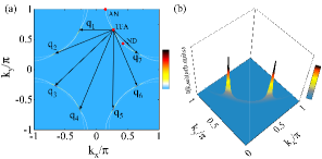
Figure 1: (Color online) (a) The electron Fermi surface map and (b) the surface plot of the homogenous quasiparticle excitation spectrum for zero energy $\omega=0$ at $\delta=0.15$ with $T=0.002J$, where AN, TFA, and ND denote the antinode, tip of the Fermi arc, and node, respectively, while ${\bf q}_{1}$, ${\bf q}_{2}$, ${\bf q}_{3}$, ${\bf q}_{4}$, ${\bf q}_{5}$, ${\bf q}_{6}$, and ${\bf q}_{7}$ indicate different scattering wave vectors.

In the previous studies Liu21 ; Gao18 , the topology of EFS in the pure system has been discussed in terms of the intensity map of the homogenous quasiparticle excitation spectrum $I({\bf k},\omega)$ at zero energy $\omega=0$, where we have shown that the formation of the disconnected Fermi arcs due to the EFS reconstruction is directly associated with the emergence of the highly anisotropic momentum-dependence of the homogenous quasiparticle scattering rate. For a convenience in the following discussions of the impurity scattering influence on the electronic structure, (a) the EFS map in the pure system and (b) the surface plot of the homogenous quasiparticle excitation spectrum for zero energy $\omega=0$ at doping $\delta=0.15$ with temperature $T=0.002J$ are replotted in Fig. 1. Obviously, the typical feature is that EFS contour is broken up into the disconnected Fermi arcs located around the nodal region Shi08 ; Sassa11 ; Comin14 ; Horio16 ; Loret18 , where a large number of the low-energy electronic states is available at around the tips of the Fermi arcs, and then all the anomalous properties arise from these quasiparticles at around the tips of the Fermi arcs Timusk99 ; Hufner08 ; Comin16 ; Vishik18 . These tips of the Fermi arcs connected by the scattering wave vectors ${\bf q}_{i}$ shown in Fig. 1 naturally construct an octet scattering model, and then the quasiparticle scattering processes with the scattering wave vectors ${\bf q}_{i}$ therefore contribute effectively to the quasiparticle scattering processes Yin21 ; Pan01 ; Hoffman02 ; Kohsaka07 ; Kohsaka08 ; Hamidian16 . As we have mentioned in section I, this octet scattering model shown in Fig. 1 can persist into the case for a finite binding-energy Chatterjee06 ; He14 , which leads to that the sharp peaks in the ARPES autocorrelation spectrum with the scattering wave vectors ${\bf q}_{i}$ are directly correlated to the regions of the highest joint density of states. We will return to this discussion of the ARPES autocorrelation towards Sec. III.3 of this paper.

II.3 Dressed electron propagator

With the help of the above homogenous electron propagator (II.1), now we can discuss the influence of the impurity scattering on the electronic structure. In the presence of impurities, the homogenous electron propagator (II.1) is dressed via the impurity scattering as Hussey02 ; Balatsky06 ; Alloul09 ,

$$\tilde{G}_{\rm I}({\bf k},\omega)^{-1}=\tilde{G}({\bf k},\omega)^{-1}-\tilde{\Sigma}_{\rm I}({\bf k},\omega),$$ (12)

where as the homogenous self-energy $\tilde{\Sigma}({\bf k},\omega)=\sum_{\alpha=0}^{3}\tilde{\Sigma}_{\alpha}({\bf k},\omega)$ in Eq. (II.1), the impurity scattering self-energy $\tilde{\Sigma}_{\rm I}({\bf k},\omega)$ can be also generally expressed as,

$$\tilde{\Sigma}_{\rm I}({\bf k},\omega)=\sum_{\alpha=0}^{3}\Sigma_{{\rm I}\alpha}({\bf k},\omega)\tau_{\alpha}$$ (15)

$$= \left(\begin{array}[]{cc}\Sigma_{\rm I0}({\bf k},\omega)+\Sigma_{\rm I3}({\bf k},\omega),&\Sigma_{\rm I1}({\bf k},\omega)-i\Sigma_{\rm I2}({\bf k},\omega)\\ \Sigma_{\rm I1}({\bf k},\omega)+i\Sigma_{\rm I2}({\bf k},\omega),&\Sigma_{\rm I0}({\bf k},\omega)-\Sigma_{\rm I3}({\bf k},\omega)\end{array}\right).~{}~{}~{}~{}~{}$$

Moreover, in corresponding to the homogenous self-energies $\Sigma_{1}({\bf k},\omega)$, $\Sigma_{2}({\bf k},\omega)$, $\Sigma_{3}({\bf k},\omega)$, and $\Sigma_{0}({\bf k},\omega)$ in Eq. (II.1), both $\Sigma_{\rm I1}({\bf k},\omega)$ and $\Sigma_{\rm I2}({\bf k},\omega)$ are real, while both $\Sigma_{\rm I3}({\bf k},\omega)$, and $\Sigma_{\rm I0}({\bf k},\omega)/\omega$ are an even function of $\omega$. Substituting this impurity scattering self-energy (15) and homogenous electron propagator (II.1) into Eq. (12), the dressed electron propagator can be expressed as,

$$\tilde{G}_{\rm I}({\bf k},\omega) = \left(\begin{array}[]{cc}G_{\rm I}({\bf k},\omega),&\Im_{\rm I}({\bf k},\omega)\\ \Im^{\dagger}_{\rm I}({\bf k},\omega),&-G_{\rm I}({\bf k},-\omega)\end{array}\right)$$

$$= {1\over F_{\rm I}({\bf k},\omega)}\{[\omega-\Sigma_{0}({\bf k},\omega)-\Sigma_{\rm I0}({\bf k},\omega)]\tau_{0}$$

$$+ [\Sigma_{1}({\bf k},\omega)+\Sigma_{\rm I1}({\bf k},\omega)]\tau_{1}$$

$$+ [\Sigma_{2}({\bf k},\omega)+\Sigma_{\rm I2}({\bf k},\omega)]\tau_{2}$$

$$+ [\varepsilon_{\bf k}+\Sigma_{3}({\bf k},\omega)+\Sigma_{\rm I3}({\bf k},\omega)]\tau_{3}\},~{}~{}$$ (19)

where $F_{\rm I}({\bf k},\omega)=[\omega-\Sigma_{0}({\bf k},\omega)-\Sigma_{\rm I0}({\bf k},\omega)]^{2}-[\varepsilon_{\bf k}+\Sigma_{3}({\bf k},\omega)+\Sigma_{\rm I3}({\bf k},\omega)]^{2}-[\Sigma_{1}({\bf k},\omega)+\Sigma_{\rm I1}({\bf k},\omega)]^{2}-[\Sigma_{2}({\bf k},\omega)+\Sigma_{\rm I2}({\bf k},\omega)]^{2}$.

II.4 Self-consistent T-matrix approach

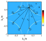
Figure 2: (Color online) The impurity scattering in the octet scattering model. $V_{1}$ is the impurity scattering potential for the intra-tip scattering, $V_{2}$, $V_{3}$, $V_{7}$, and $V_{8}$ are the impurity scattering potentials for the adjacent-tip scattering, while $V_{4}$, $V_{5}$, and $V_{6}$ are the impurity scattering potentials for the opposite-tip scattering. The tips of the Fermi arcs (then the scattering centers) are divided into two groups: (A) the tips of the Fermi arcs located at the region of $|k_{y}|>|k_{x}|$ and (B) the tips of the Fermi arcs located at the region of $|k_{x}|>|k_{y}|$.

Starting from the homogenous part of the BCS-like electron propagator with the d-wave symmetry, it has been shown that the self-consistent $T$-matrix approach is a powerful tool to treat the impurity scattering in the SC-state for an arbitrary scattering strength Hussey02 ; Balatsky06 ; Alloul09 ; Mahan81 ; Hirschfeld89 ; Hirschfeld93 . In the following discussions, we employ the self-consistent $T$-matrix approach to analyze the impurity scattering self-energy $\tilde{\Sigma}_{\rm I}({\bf k},\omega)$ in Eq. (15) in terms of the dressed electron propagator (II.3). Following the self-consistent $T$-matrix approach Hussey02 ; Balatsky06 ; Alloul09 ; Mahan81 ; Hirschfeld89 ; Hirschfeld93 , the impurity scattering self-energy (15) can be expressed approximately as,

$$\tilde{\Sigma}_{\rm I}({\bf k},\omega)=n_{\rm i}N\tilde{T}_{{\bf k}{\bf k}}(\omega),$$ (20)

where $n_{\rm i}$ is the impurity concentration, $N$ is the number of sites on a square lattice, and $\tilde{T}_{{\bf k}{\bf k}}(\omega)$ is the diagonal part of the T-matrix, while the T-matrix is given by the summation of all impurity scattering processes as,

$$\tilde{T}_{{\bf k}{\bf k}^{\prime}}={1\over N}\tau_{3}V_{{\bf k}{\bf k}^{\prime}}+{1\over N}\sum_{{\bf k}^{\prime\prime}}V_{{\bf k}{\bf k}^{\prime\prime}}\tau_{3}\tilde{G}_{\rm I}({\bf k}^{\prime\prime},\omega)\tilde{T}_{{\bf k}^{\prime\prime}{\bf k}^{\prime}},$$ (21)

with the impurity scattering potential $V_{{\bf k}{\bf k}^{\prime}}$, where we have followed the common practice Hussey02 ; Balatsky06 ; Alloul09 ; Mahan81 ; Hirschfeld89 ; Hirschfeld93 , and treated the impurity scattering potential $V_{{\bf k}{\bf k}^{\prime}}$ in the static-limit for a qualitative understanding of the influence of impurities on the low-energy electronic structure of cuprate superconductors.

In the octet scattering model shown in Fig. 1, a large number of the low-energy electronic states is located at around eight tips of the Fermi arcs. In other words, the most quasiparticles are generated only at around these tips of the Fermi arcs. This characteristic feature is very helpful when one considers the impurity scattering, since the initial and final momenta of a scattering event must always be approximately equal to the ${\bf k}$-space located at around one of these tips of the Fermi arcs in the case of low-temperature and low-energy. On the other hand, the impurity scattering potential $V_{{\bf k}{\bf k}^{\prime}}$ varies slowly over the area around the tip of the Fermi arc, and thus the impurity scattering potential can be approximated to be identical within one half of each quarter in the Brillouin zone (BZ). In this case, a general impurity scattering potential $V_{{\bf k}{\bf k}^{\prime}}$ in Eq. (21) need mainly to be considered in three possible cases as shown in Fig. 2: (i) the impurity scattering potential for the scattering at the intra-tip of the Fermi arc $V_{{\bf k}{\bf k}^{\prime}}=V_{1}$ (${\bf k}$ and ${\bf k}^{\prime}$ at the same tip of the Fermi arc); (ii) the impurity scattering potentials for the scattering at the adjacent-tips of the Fermi arcs $V_{{\bf k}{\bf k}^{\prime}}=V_{2}$, $V_{{\bf k}{\bf k}^{\prime}}=V_{3}$, $V_{{\bf k}{\bf k}^{\prime}}=V_{7}$, and $V_{{\bf k}{\bf k}^{\prime}}=V_{8}$ (${\bf k}$ and ${\bf k}^{\prime}$ at the adjacent-tips of the Fermi arcs); (iii) and the impurity scattering potentials for the scattering at the opposite-tips of the Fermi arcs $V_{{\bf k}{\bf k}^{\prime}}=V_{4}$, $V_{{\bf k}{\bf k}^{\prime}}=V_{5}$, and $V_{{\bf k}{\bf k}^{\prime}}=V_{6}$ (${\bf k}$ and ${\bf k}^{\prime}$ at the opposite-tips of the Fermi arcs). This approximation based on the octet scattering model is so-called as the Fermi-arc-tip approximation. It should be emphasized that in this Fermi-arc-tip approximation, the influence of the impurity scattering on the electron pair strength can be explored directly, which is much different from the case in the nodal approximation Hussey02 ; Balatsky06 ; Alloul09 . In this Fermi-arc-tip approximation, the impurity scattering potential $V_{{\bf k}{\bf k}^{\prime}}$ in the self-consistent T-matrix equation (21) is dependent on the momenta at the tips of the Fermi arcs only, and can be effectively reduced as a $8\times 8$-matrix,

$$\tilde{V}=\left(\begin{array}[]{cccc}V_{11}&V_{12}&\cdots&V_{18}\\ V_{21}&V_{22}&\cdots&V_{28}\\ \vdots&\vdots&\ddots&\vdots\\ V_{81}&V_{82}&\cdots&V_{88}\end{array}\right),$$ (26)

where the matrix elements are given by: $V_{jj}=V_{1}$ for $j=1,2,3,...8$, $V_{jj^{\prime}}=V_{j^{\prime}j}=V_{2}$ for $j=1,2,3,6$ with the corresponding $j^{\prime}=7,4,5,8$, respectively, $V_{jj^{\prime}}=V_{j^{\prime}j}=V_{3}$ for $j=1,2,3,4$ with the corresponding $j^{\prime}=8,7,6,5$, respectively, $V_{jj^{\prime}}=V_{jj^{\prime}}=V_{4}$ for $j=1,2,3,4$ with the corresponding $j^{\prime}=6,5,8,7$, respectively, $V_{jj^{\prime}}=V_{j^{\prime}j}=V_{5}$ for $j=1,2,3,4$ with the corresponding $j^{\prime}=5,6,7,8$, respectively, $V_{jj^{\prime}}=V_{j^{\prime}j}=V_{6}$ for $j=1,2,4,5$ with the corresponding $j^{\prime}=3,8,6,7$, respectively, $V_{jj^{\prime}}=V_{j^{\prime}j}=V_{7}$ for $j=1,2,5,6$ with the corresponding $j^{\prime}=4,3,8,7$, respectively, and $V_{jj^{\prime}}=V_{j^{\prime}j}=V_{8}$, for $j=1,3,5,7$ with the corresponding $j^{\prime}=2,4,6,8$, respectively.

At the case of zero temperature and zero energy, the Fermi arc collapses to the point at the tip of the Fermi arc, leading to form the Fermi-arc-tip liquid Liu21 ; Gao18 , where all the spectral weights on the Fermi arc are reduced to the point at the tip of the Fermi arc, indicating that the quasiparticles are only generated at the tips of the Fermi arcs and the rest of BZ makes no contribution. In this case, the scattering processes in the octet scattering model shown in Fig. 2 represent all the scattering processes in the system, and then in principle, the Fermi-arc-tip approximation for the impurity scattering potentials can reproduce properly any impurity scattering potential with arbitrary strength, especially the adjacent scattering potential for the scattering at two different tips of the Fermi arcs. On the other hand, at the case of low-temperature and low-energy, although the spectral weight on the point at the tip of the Fermi arc spreads on the extremely small area around the point at the tip of the Fermi arc, the characteristic feature of the Fermi arc with the most part of the spectral weight located around the point at tip of the Fermi arc remains Chatterjee06 ; He14 ; Gao18a ; Gao19 , indicating that the Fermi-arc-tip approximation is still appropriate to treat the impurity scattering at the case of low-temperature and low-energy. In the following discussions, we therefore employ the reduced impurity scattering potential (26) to study the influence of the impurity scattering on the electronic structure. Substituting the impurity scattering potential $\tilde{V}$ in Eq. (26) into Eq. (21), the T-matrix equation can be expressed explicitly as a $16\times 16$-matrix equation around eight tips of the Fermi arcs as,

$$\tilde{T}_{jj^{\prime}}={1\over N}\tau_{3}V_{jj^{\prime}}+{1\over N}\sum_{j^{\prime\prime}{\bf k}^{\prime\prime}}V_{jj^{\prime\prime}}[\tau_{3}\tilde{G}_{\rm I}({\bf k}^{\prime\prime},\omega)]\tilde{T}_{j^{\prime\prime}j^{\prime}},$$ (27)

where $j$, $j^{\prime}$, and $j^{\prime\prime}$ are labels of the tips of the Fermi arcs, the summation ${\bf k}^{\prime\prime}$ is over the area around the tip $j^{\prime\prime}$ of the Fermi arc, and then the impurity scattering self-energy $\tilde{\Sigma}_{\rm I}({\bf k},\omega)$ in Eq. (20) is reduced as,

$$\tilde{\Sigma}_{\rm I}(\omega)=n_{\rm i}N\tilde{T}_{jj}(\omega),$$ (28)

and therefore is also dependent on the momenta at the tips of the Fermi arcs only.

It should be noted that the typical feature of the octet scattering model shown in Fig. 1 is that two tips of the Fermi arc in each quarter of BZ is symmetrical about the nodal (diagonal) direction, reflecting a basic fact that the diagonal propagator in Eq. (II.1) is symmetrical about the nodal direction. However, the off-diagonal propagator in Eq. (II.1) is asymmetrical about the nodal direction, since the homogenous self-energies $\Sigma_{1}({\bf k},\omega)$ and $\Sigma_{2}({\bf k},\omega)$ in the particle-particle channel (then the momentum and energy dependence of the homogenous SC gap) have a d-wave symmetry in the framework of the kinetic-energy-driven superconductivity. In this case, we can divide the region of the location of the tips of the Fermi arcs (then the scattering centers) into two groups: (A) the tips of the Fermi arcs located at the region of $|k_{y}|>|k_{x}|$ and (B) the tips of the Fermi arcs located at the region of $|k_{x}|>|k_{y}|$. Since the symmetry of the impurity scattering self-energy $\tilde{\Sigma}_{\rm I}(\omega)$ is the same as the homogenous self-energy $\tilde{\Sigma}({\bf k},\omega)$, the dressed electron propagator $\tilde{G}_{I}({\bf k},\omega)$ in Eq. (12) can be expressed explicitly in the regions A and B as,

$$\tilde{G}^{\rm(A)}_{\rm I}({\bf k},\omega) = \left(\begin{array}[]{cc}G^{\rm(A)}_{\rm I}({\bf k},\omega),&\Im^{\rm(A)}_{\rm I}({\bf k},\omega)\\ \Im^{{\rm(A)}\dagger}_{\rm I}({\bf k},\omega),&-G^{\rm(A)}_{\rm I}({\bf k},-\omega)\end{array}\right)$$

$$= {1\over F^{\rm(A)}_{\rm I}({\bf k},\omega)}\{[\omega-\Sigma_{0}({\bf k},\omega)-\Sigma_{\rm I0}(\omega)]\tau_{0}$$

$$+ [\Sigma_{1}({\bf k},\omega)+\Sigma^{\rm(A)}_{\rm I1}(\omega)]\tau_{1}$$

$$+ [\Sigma_{2}({\bf k},\omega)+\Sigma^{\rm(A)}_{\rm I2}(\omega)]\tau_{2}$$

$$+ [\varepsilon_{\bf k}+\Sigma_{3}({\bf k},\omega)+\Sigma_{\rm I3}(\omega)]\tau_{3}\},~{}~{}$$ (29d)

$$\tilde{G}^{\rm(B)}_{\rm I}({\bf k},\omega) = \left(\begin{array}[]{cc}G^{\rm(B)}_{\rm I}({\bf k},\omega),&\Im^{\rm(B)}_{\rm I}({\bf k},\omega)\\ \Im^{{\rm(B)}\dagger}_{\rm I}({\bf k},\omega),&-G^{\rm(B)}_{\rm I}({\bf k},-\omega)\end{array}\right)$$

$$= {1\over F^{\rm(B)}_{\rm I}({\bf k},\omega)}\{[\omega-\Sigma_{0}({\bf k},\omega)-\Sigma_{\rm I0}(\omega)]\tau_{0}$$

$$+ [\Sigma_{1}({\bf k},\omega)+\Sigma^{\rm(B)}_{\rm I1}(\omega)]\tau_{1}$$

$$+ [\Sigma_{2}({\bf k},\omega)+\Sigma^{\rm(B)}_{\rm I2}(\omega)]\tau_{2}$$

$$+ [\varepsilon_{\bf k}+\Sigma_{3}({\bf k},\omega)+\Sigma_{\rm I3}(\omega)]\tau_{3}\},~{}~{}$$ (29h)

respectively, where $F^{\rm(A)}_{\rm I}({\bf k},\omega)=[\omega-\Sigma_{0}({\bf k},\omega)-\Sigma_{\rm I0}(\omega)]^{2}-[\varepsilon_{\bf k}+\Sigma_{3}({\bf k},\omega)+\Sigma_{\rm I3}(\omega)]^{2}-[\Sigma_{1}({\bf k},\omega)+\Sigma^{\rm(A)}_{\rm I1}(\omega)]^{2}-[\Sigma_{2}({\bf k},\omega)+\Sigma^{\rm(A)}_{\rm I2}(\omega)]^{2}$, $F^{\rm(B)}_{\rm I}({\bf k},\omega)=[\omega-\Sigma_{0}({\bf k},\omega)-\Sigma_{\rm I0}(\omega)]^{2}-[\varepsilon_{\bf k}+\Sigma_{3}({\bf k},\omega)+\Sigma_{\rm I3}(\omega)]^{2}-[\Sigma_{1}({\bf k},\omega)+\Sigma^{\rm(B)}_{\rm I1}(\omega)]^{2}-[\Sigma_{2}({\bf k},\omega)+\Sigma^{\rm(B)}_{\rm I2}(\omega)]^{2}$. With the help of the above dressed electron propagators $\tilde{G}^{\rm(A)}_{I}({\bf k},\omega)$ and $\tilde{G}^{\rm(B)}_{I}({\bf k},\omega)$, the self-consistent T-matrix equation (27) can be further reduced as,

$$\tilde{T}_{jj^{\prime}} = {1\over N}V_{jj^{\prime}}\tau_{3}+{1\over N}\sum_{j^{\prime\prime}\in{\rm A}}V_{jj^{\prime\prime}}[\tau_{3}\tilde{I}^{\rm(A)}_{\tilde{G}}(\omega)]\tilde{T}_{j^{\prime\prime}j^{\prime}}$$ (30)

$$+ {1\over N}\sum_{j^{\prime\prime}\in{\rm B}}V_{jj^{\prime\prime}}[\tau_{3}\tilde{I}^{\rm(B)}_{\tilde{G}}(\omega)]\tilde{T}_{j^{\prime\prime}j^{\prime}},$$

where $\tilde{I}^{\rm(A)}_{\tilde{G}}(\omega)$ and $\tilde{I}^{\rm(B)}_{\tilde{G}}(\omega)$ are the integral propagators, and can be expressed explicitly as,

$$\tilde{I}^{\rm(A)}_{\tilde{G}}(\omega) = \sum_{{\bf k}\in{\rm A}}\tilde{G}^{\rm(A)}_{\rm I}({\bf k},\omega)=\sum\limits_{\alpha=0}^{3}\tau_{\alpha}I^{\rm(A)}_{\tilde{G}\alpha}(\omega),$$ (31)

$$\tilde{I}^{\rm(B)}_{\tilde{G}}(\omega) = \sum_{{\bf k}\in{\rm B}}\tilde{G}^{\rm(B)}_{\rm I}({\bf k},\omega)=\sum\limits_{\alpha=0}^{3}\tau_{\alpha}I^{\rm(B)}_{\tilde{G}\alpha}(\omega),~{}~{}~{}$$ (32)

respectively. To coincide with the separation of the region of the location of the Fermi-arc tips, the matrix of the impurity scattering potential $\tilde{V}$ in Eq. (26) now can be rearranged in the following way,

$${1\over N}\tilde{V}=\left(\begin{array}[]{cc}\bar{V}_{\rm AA}&\bar{V}_{\rm AB}\\ \bar{V}_{\rm BA}&\bar{V}_{\rm BB}\end{array}\right),$$ (35)

with the $4\times 4$-matrices of the impurity scattering potentials $\bar{V}_{\rm AA}$, $\bar{V}_{\rm AB}$, $\bar{V}_{\rm BA}$, and $\bar{V}_{\rm BB}$ that are given by,

$$\bar{V}_{\rm AA} = {1\over N}\left(\begin{array}[]{cccc}V_{11}&V_{13}&V_{15}&V_{17}\\ V_{31}&V_{33}&V_{35}&V_{37}\\ V_{51}&V_{53}&V_{55}&V_{57}\\ V_{71}&V_{73}&V_{75}&V_{77}\end{array}\right),$$ (36e)

$$\bar{V}_{\rm AB} = {1\over N}\left(\begin{array}[]{cccc}V_{12}&V_{14}&V_{16}&V_{18}\\ V_{32}&V_{34}&V_{36}&V_{38}\\ V_{52}&V_{54}&V_{56}&V_{58}\\ V_{72}&V_{74}&V_{76}&V_{78}\end{array}\right),$$ (36j)

$$\bar{V}_{\rm BA} = {1\over N}\left(\begin{array}[]{cccc}V_{21}&V_{23}&V_{25}&V_{27}\\ V_{41}&V_{43}&V_{45}&V_{47}\\ V_{61}&V_{63}&V_{65}&V_{67}\\ V_{81}&V_{83}&V_{85}&V_{87}\end{array}\right),$$ (36o)

$$\bar{V}_{\rm BB} = {1\over N}\left(\begin{array}[]{cccc}V_{22}&V_{24}&V_{26}&V_{28}\\ V_{42}&V_{44}&V_{46}&V_{48}\\ V_{62}&V_{64}&V_{66}&V_{68}\\ V_{82}&V_{84}&V_{86}&V_{88}\end{array}\right),~{}~{}~{}~{}~{}~{}~{}~{}$$ (36t)

respectively. According to the above impurity scattering potential $\tilde{V}$ in Eq. (35), the self-consistent T-matrix equation (30) then can be rewritten as,

$$\tilde{T}_{\mu\nu} = \bar{V}_{\mu\nu}\otimes\tau_{3}+\bar{V}_{\mu{\rm A}}\otimes[\tau_{3}\tilde{I}^{\rm(A)}_{\tilde{G}}(\omega)]\tilde{T}_{{\rm A}\nu}$$ (37)

$$+ \bar{V}_{\mu{\rm B}}\otimes[\tau_{3}\tilde{I}^{\rm(A)}_{\tilde{G}}(\omega)]\tilde{T}_{{\rm B}\nu},$$

where $\mu$ ($\nu$) denotes region A or B. After a quite complicated calculation, the above T-matrix equation now can be evaluated as [see Appendix A],

$$\sum\limits_{\alpha=0}^{3}T^{(\alpha)}_{\mu\nu}\otimes\tau_{\alpha}\tau_{3}=\sum\limits_{\alpha=0}^{3}\big{(}\sum\limits_{\mu^{\prime}={\rm A},{\rm B}}\bar{V}_{\mu\mu^{\prime}}\bar{\Lambda}^{(\alpha)}_{\mu^{\prime}\nu}\big{)}\otimes\tau_{\alpha},$$ (38)

with the matrix $\bar{\Lambda}^{(\alpha)}$,

$$\bar{\Lambda}^{(\alpha)}\otimes\tau_{\alpha}=\bar{M}={1\over 1-\tilde{M}},$$ (39)

where the matrix $\tilde{M}$ is obtained as,

$$\tilde{M} = \left(\begin{array}[]{cc}\bar{V}_{\rm AA}\otimes\tau_{3}\tilde{I}^{\rm(A)}_{\tilde{G}}(\omega),&\bar{V}_{\rm AB}\otimes\tau_{3}\tilde{I}^{\rm(A)}_{\tilde{G}}(\omega)\\ \bar{V}_{\rm BA}\otimes\tau_{3}\tilde{I}^{\rm(B)}_{\tilde{G}}(\omega),&\bar{V}_{\rm BB}\otimes\tau_{3}\tilde{I}^{\rm(B)}_{\tilde{G}}(\omega)\end{array}\right),~{}~{}~{}~{}~{}$$ (42)

and then the elements in the matrix $\bar{\Lambda}^{(\alpha)}$ are given by,

$$\Lambda^{(0)}_{\tfrac{i+1}{2}\tfrac{i^{\prime}+1}{2}} = \frac{1}{2}(\bar{M}_{ii^{\prime}}+\bar{M}_{i+1i^{\prime}+1}),$$ (43a)

$$\Lambda^{(3)}_{\tfrac{i+1}{2}\tfrac{i^{\prime}+1}{2}} = \frac{1}{2}(\bar{M}_{ii^{\prime}}-\bar{M}_{i+1i^{\prime}+1}),$$ (43b)

$$\Lambda^{(1)}_{\tfrac{i+1}{2}\tfrac{i^{\prime}+1}{2}} = \frac{1}{2}(\bar{M}_{ii^{\prime}+1}+\bar{M}_{i+1i^{\prime}}),$$ (43c)

$$\Lambda^{(2)}_{\tfrac{i+1}{2}\tfrac{i^{\prime}+1}{2}} = \frac{i}{2}(\bar{M}_{ii^{\prime}+1}-\bar{M}_{i+1i^{\prime}}),$$ (43d)

with $i$ ($i^{\prime}$)=1,3, 5, $\cdots$, 15. The solution of this T-matrix equation (38) now is given straightforwardly as,

$$T_{\mu\nu}^{(0)}(\omega) = \sum\limits_{\mu^{\prime}={\rm A},{\rm B}}\bar{V}_{\mu\mu^{\prime}}\bar{\Lambda}^{(3)}_{\mu^{\prime}\nu},$$ (44a)

$$T_{\mu\nu}^{(1)}(\omega) = i\sum\limits_{\mu^{\prime}={\rm A},{\rm B}}\bar{V}_{\mu\mu^{\prime}}\bar{\Lambda}^{(2)}_{\mu^{\prime}\nu},$$ (44b)

$$T_{\mu\nu}^{(2)}(\omega) = -i\sum\limits_{\mu^{\prime}={\rm A},{\rm B}}\bar{V}_{\mu\mu^{\prime}}\bar{\Lambda}^{(1)}_{\mu^{\prime}\nu},$$ (44c)

$$T_{\mu\nu}^{(3)}(\omega) = \sum\limits_{\mu^{\prime}={\rm A},{\rm B}}\bar{V}_{\mu\mu^{\prime}}\bar{\Lambda}^{(0)}_{\mu^{\prime}\nu}.$$ (44d)

Following this solution of the T-matrix equation, the impurity scattering self-energy $\tilde{\Sigma}_{\rm I}(\omega)=\sum\limits_{\alpha=0}^{3}\Sigma_{{\rm I}\alpha}(\omega)\tau_{\alpha}=n_{i}N\tilde{T}_{jj}(\omega)$ in the region A can be obtained as,

$$\Sigma^{\rm(A)}_{\rm I0}(\omega) = n_{i}N(T_{\rm AA}^{(0)})_{11}=Nn_{i}(\sum\limits_{\mu^{\prime}={\rm A},{\rm B}}\bar{V}_{{\rm A}\mu^{\prime}}\bar{\Lambda}^{(3)}_{\mu^{\prime}{\rm A}})_{11},~{}~{}~{}~{}~{}~{}$$ (45a)

$$\Sigma^{\rm(A)}_{\rm I1}(\omega) = n_{i}N{\rm Re}(T_{\rm AA}^{(1)})_{11}$$ (45b)

$$= -Nn_{i}{\rm Im}(\sum\limits_{\mu^{\prime}={\rm A},{\rm B}}\bar{V}_{{\rm A}\mu^{\prime}}\bar{\Lambda}^{(2)}_{\mu^{\prime}{\rm A}})_{11},$$

$$\Sigma^{\rm(A)}_{\rm I2}(\omega) = n_{i}N{\rm Re}(T_{\rm AA}^{(2)})_{11}$$ (45c)

$$= Nn_{i}{\rm Im}(\sum\limits_{\mu^{\prime}={\rm A},{\rm B}}\bar{V}_{{\rm A}\mu^{\prime}}\bar{\Lambda}^{(1)}_{\mu^{\prime}{\rm A}})_{11},~{}~{}~{}~{}~{}$$

$$\Sigma^{\rm(A)}_{\rm I3}(\omega) = n_{i}N(T_{\rm AA}^{(3)})_{11}=Nn_{i}(\sum\limits_{\mu^{\prime}={\rm A},{\rm B}}\bar{V}_{{\rm A}\mu^{\prime}}\bar{\Lambda}^{(0)}_{\mu^{\prime}{\rm A}})_{11},~{}~{}~{}~{}~{}$$ (45d)

and in the region B is given by,

$$\Sigma^{\rm(B)}_{\rm I0}(\omega) = n_{i}N(T_{\rm BB}^{(0)})_{11}=Nn_{i}(\sum\limits_{\mu^{\prime}={\rm A},{\rm B}}\bar{V}_{{\rm B}\mu^{\prime}}\bar{\Lambda}^{(3)}_{\mu^{\prime}{\rm B}})_{11},~{}~{}~{}~{}~{}~{}~{}$$ (46a)

$$\Sigma^{\rm(B)}_{\rm I1}(\omega) = n_{i}N{\rm Re}(T_{\rm BB}^{(1)})_{11}$$ (46b)

$$= -Nn_{i}{\rm Im}(\sum\limits_{\mu^{\prime}={\rm A},{\rm B}}\bar{V}_{{\rm B}\mu^{\prime}}\bar{\Lambda}^{(2)}_{\mu^{\prime}{\rm B}})_{11},$$

$$\Sigma^{\rm(B)}_{\rm I2}(\omega) = n_{i}N{\rm Re}(T_{\rm BB}^{(2)})_{11}$$ (46c)

$$= Nn_{i}{\rm Im}(\sum\limits_{\mu^{\prime}={\rm A},{\rm B}}\bar{V}_{{\rm B}\mu^{\prime}}\bar{\Lambda}^{(1)}_{mu^{\prime}{\rm B}})_{11},~{}~{}~{}~{}~{}$$

$$\Sigma^{\rm(B)}_{\rm I3}(\omega) = n_{i}N(T_{\rm BB}^{(3)})_{11}=Nn_{i}(\sum\limits_{\mu^{\prime}={\rm A},{\rm B}}\bar{V}_{{\rm B}\mu^{\prime}}\bar{\Lambda}^{(0)}_{\mu^{\prime}{\rm B}})_{11}.~{}~{}~{}~{}~{}~{}~{}~{}$$ (46d)

The above impurity scattering self-energies in Eqs. (45) and (46) are obtained firstly in the Fermi-arc-tip approximation of the quasiparticle excitations and scattering processes based on a microscopic octet scattering model.

Since the self-energy in the particle-hole channel is symmetrical about the nodal direction and the self-energy in the particle-particle channel is asymmetrical about the nodal direction, the above impurity scattering self-energies in the regions A and B can be rewritten uniformly as,

$$\Sigma^{\rm(A)}_{\rm I0}(\omega) = \Sigma^{\rm(B)}_{\rm I0}(\omega)=\Sigma_{\rm I0}(\omega),$$ (47a)

$$\Sigma^{\rm(A)}_{\rm I1}(\omega) = -\Sigma^{\rm(B)}_{\rm I1}(\omega)=\Sigma_{\rm I1}(\omega),$$ (47b)

$$\Sigma^{\rm(A)}_{\rm I2}(\omega) = -\Sigma^{\rm(B)}_{\rm I2}(\omega)=\Sigma_{\rm I2}(\omega),$$ (47c)

$$\Sigma^{\rm(A)}_{\rm I3}(\omega) = \Sigma^{\rm(B)}_{\rm I3}(\omega)=\Sigma_{\rm I3}(\omega),$$ (47d)

and then the dressed quasiparticle excitation spectrum now can be obtained as,

$$I_{\rm I}({\bf k},\omega)=|M({\bf k},\omega)|^{2}n_{\rm F}(\omega)A_{\rm I}({\bf k},\omega),$$ (48)

where the dressed electron spectral function $A_{\rm I}({\bf k},\omega)$ is obtained directly from the dressed electron propagator (II.3) as,

$$A_{\rm I}({\bf k},\omega)=-2{\rm Im}G_{\rm I}({\bf k},\omega)$$ (49)

$$= {-2{\rm Im}\Sigma^{\rm(IM)}_{\rm tot}({\bf k},\omega)\over[\omega-\varepsilon_{\bf k}-{\rm Re}\Sigma^{\rm(IM)}_{\rm tot}({\bf k},\omega)]^{2}+[{\rm Im}\Sigma^{\rm(IM)}_{\rm tot}({\bf k},\omega)]^{2}},~{}~{}~{}~{}~{}~{}~{}~{}~{}$$

with ${\rm Re}\Sigma^{\rm(IM)}_{\rm tot}({\bf k},\omega)$ and ${\rm Im}\Sigma^{\rm(IM)}_{\rm tot}({\bf k},\omega)$ that are the real and imaginary parts of the total dressed self-energy,

$$\Sigma^{\rm(IM)}_{\rm tot}({\bf k},\omega) = \Sigma_{\rm ph}({\bf k},\omega)+\Sigma^{\rm(I)}_{\rm ph}(\omega)$$ (50)

$$+ {|\Sigma_{\rm pp}({\bf k},\omega)+(-1)^{\mu+1}\Sigma^{\rm(I)}_{\rm pp}(\omega)|^{2}\over\omega+\varepsilon_{\bf k}+\Sigma_{\rm ph}({\bf k},-\omega)+\Sigma^{\rm(I)}_{\rm ph}(-\omega)},~{}~{}~{}~{}~{}~{}~{}$$

respectively, where $\mu=1,2$ for the regions A and B, respectively, $\Sigma^{\rm(I)}_{\rm ph}(\omega)=\Sigma_{\rm I0}(\omega)+\Sigma_{\rm I3}(\omega)$ and $\Sigma^{\rm(I)}_{\rm pp}(\omega)=\Sigma_{\rm I1}(\omega)-i\Sigma_{\rm I2}(\omega)$ are the impurity scattering self-energies in the particle-hole and particle-particle channels, respectively. In the previous studies based on the nodal approximation of the quasiparticle excitations and scattering processes Hussey02 ; Balatsky06 ; Alloul09 , the reasonable strengths of the intra-node impurity scattering, the adjacent-node impurity scattering, and the opposite-node impurity scattering have been used to discuss the influence of the impurity scattering on various properties of the SC-state in cuprate superconductors Durst00 ; Yashenkin01 ; Nunner05 ; Dahm05 ; Wang08 ; Andersen08 ; Wang09 ; Hone17 . Unless otherwise indicated, the strengths of the intra-tip impurity scattering $V_{1}$, the adjacent-tip impurity scattering $V_{2}$, $V_{3}$, $V_{7}$, and $V_{8}$, and the opposite-tip impurity scattering $V_{4}$, $V_{5}$, and $V_{6}$ in the following discussions are chosen as $V_{1}=58J$, $V_{2}=0.85V_{1}$, $V_{3}=0.8V_{1}$, $V_{7}=0.85V_{1}$, $V_{8}=0.9V_{1}$, $V_{4}=0.7V_{1}$, $V_{5}=0.65V_{1}$, and $V_{6}=0.75V_{1}$, respectively, to compare with the previous discussions in the nodal approximation of the quasiparticle excitations and scattering processes Durst00 ; Wang08 .

III Quantitative characteristics

The studies of the influence of the impurity scattering on the electronic structure can offer insight into the fundamental aspects of the quasiparticle excitation in cuprate superconductors Hussey02 ; Balatsky06 ; Alloul09 , and therefore also can offer points of the reference against which theories may be compared. In this section, we analyze the quantitative characteristics of the influence of the impurity scattering on the electronic structure of cuprate superconductors in the SC-state to shed light on the nature of the SC-state quasiparticle excitation.

III.1 Impurity concentration dependence of impurity scattering self-energy

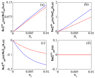
Figure 3: (Color online) (a) The real part and (b) the imaginary part of the impurity scattering self-energy in the particle-hole channel and (c) the real part and (d) the imaginary part of the impurity scattering self-energy in the particle-particle channel at the antinode as a function of the impurity concentration at $\delta=0.15$ with $T=0.002J$ in zero energy $\omega=0$ for the strengths of the adjacent-tip impurity scattering $V_{2}=0.85V_{1}$, $V_{3}=0.8V_{1}$, $V_{7}=0.85V_{1}$, and $V_{8}=0.9V_{1}$, and the opposite-tip impurity scattering $V_{4}=0.7V_{1}$, $V_{5}=0.65V_{1}$, and $V_{6}=0.75V_{1}$, and the intra-tip impurity scattering $V_{1}=58J$ (blue-line) and $V_{1}=30J$ (red-line). ${\rm Re}\Sigma_{\rm ph}({\bf k},\omega)$ and ${\rm Im}\Sigma_{\rm ph}({\bf k},\omega)$ are the corresponding real and imaginary parts of the homogenous self-energy in the particle-hole channel, while ${\rm Re}\Sigma_{\rm pp}({\bf k},\omega)$ is the corresponding real part of the homogenous self-energy in the particle-particle channel.

In the framework of the kinetic-energy-driven superconductivity Feng0306 ; Feng12 ; Feng15a ; Feng15 , the electrons interact strongly with spin excitations resulting in the formation of the quasiparticles, and then all the unconventional features in the pure cuprate superconductors are mainly dominated by these quasiparticle behaviors Timusk99 ; Hufner08 ; Comin16 ; Vishik18 . The quasiparticle energy and lifetime in the pure system are mainly determined by the real and imaginary parts of the homogenous self-energy in the particle-hole channel, respectively, while the homogenous self-energy in the particle-particle channel is identified as the energy and momentum dependence of the homogenous SC gap in the quasiparticle excitation spectrum, and therefore is corresponding to the energy for breaking an electron pair. However, the coupling between these quasiparticles in the pure system and impurities leads to a further renormalization of both the energy and lifetime of the quasiparticles. To see this further renormalization more clearly, we firstly analyze the characteristic features of the impurity concentration dependence of the impurity scattering self-energy. In Fig. 3, we plot (a) the real part ${\rm Re}\Sigma^{\rm(I)}_{\rm ph}(\omega)$ and (b) the imaginary part ${\rm Im}\Sigma^{\rm(I)}_{\rm ph}(\omega)$ of the impurity scattering self-energy $\Sigma^{\rm(I)}_{\rm ph}(\omega)$ in the particle-hole channel and (c) the real part ${\rm Re}\Sigma^{\rm(I)}_{\rm pp}(\omega)$ and (d) the imaginary part ${\rm Im}\Sigma^{\rm(I)}_{\rm pp}(\omega)$ of the impurity scattering self-energy $\Sigma^{\rm(I)}_{\rm pp}(\omega)$ in the particle-particle channel at the antinode as a function of the impurity concentration at $\delta=0.15$ with $T=0.002J$ in zero energy $\omega=0$ for the strengths of the adjacent-tip impurity scattering $V_{2}=0.85V_{1}$, $V_{3}=0.8V_{1}$, $V_{7}=0.85V_{1}$, and $V_{8}=0.9V_{1}$, and the opposite-tip impurity scattering $V_{4}=0.7V_{1}$, $V_{5}=0.65V_{1}$, and $V_{6}=0.75V_{1}$, and the intra-tip impurity scattering $V_{1}=58J$ (blue-line) and $V_{1}=30J$ (red-line). The main features of the impurity scattering self-energy in Fig. 3 can be summarized as: (i) the values of both ${\rm Re}\Sigma^{\rm(I)}_{\rm ph}(\omega)/{\rm Re}\Sigma_{\rm ph}({\bf k},\omega)$ and ${\rm Im}\Sigma^{\rm(I)}_{\rm ph}(\omega)/{\rm Im}\Sigma_{\rm ph}({\bf k},\omega)$ are positive, indicating that the binding-energy in the pure system is shifted by ${\rm Re}\Sigma^{\rm(I)}_{\rm ph}(\omega)$ and the dispersion is further broadened by ${\rm Im}\Sigma^{\rm(I)}_{\rm ph}(\omega)$, where ${\rm Re}\Sigma_{\rm ph}({\bf k},\omega)$ and ${\rm Im}\Sigma_{\rm ph}({\bf k},\omega)$ are the corresponding real and imaginary parts of the homogenous self-energy in the particle-hole channel. In particular, with the increase of the impurity concentration, the magnitudes of both ${\rm Re}\Sigma^{\rm(I)}_{\rm ph}(\omega)/{\rm Re}\Sigma_{\rm ph}({\bf k},\omega)$ and ${\rm Im}\Sigma^{\rm(I)}_{\rm ph}(\omega)/{\rm Im}\Sigma_{\rm ph}({\bf k},\omega)$ are linearly raised Vobornik00 , which leads to a linear suppression of the spectral weight of the quasiparticle excitation spectrum and a linear reduction of the lifetime of the quasiparticle Vobornik99 ; Vobornik00 ; Shen04 ; Kondo07 ; Pan09 . (ii) for an any given impurity concentration, although the magnitude of ${\rm Im}\Sigma^{\rm(I)}_{\rm pp}(\omega)$ is equal to zero, ${\rm Re}\Sigma^{\rm(I)}_{\rm pp}(\omega)/{\rm Re}\Sigma_{\rm pp}({\bf k},\omega)$ has a negative value, where ${\rm Re}\Sigma_{\rm pp}({\bf k},\omega)$ is the corresponding real part of the homogenous self-energy in the particle-particle channel. However, the absolute value of ${\rm Re}\Sigma^{\rm(I)}_{\rm pp}(\omega)/{\rm Re}\Sigma_{\rm pp}({\bf k},\omega)$ is found to monotonically increase as the impurity concentration is increased. The kinetic-energy-driven SC-state in the pure system Feng15a is characterized by the d-wave SC gap $\bar{\Delta}_{\rm d}({\bf k},\omega)=\Sigma_{\rm pp}({\bf k},\omega)=\bar{\Delta}_{\rm d}(\omega)[{\rm cos}k_{x}-{\rm cos}k_{y}]/2$, which crosses through zero at each of four nodes on EFS ($k_{x}=\pm k_{y}$). However, the present result of ${\rm Re}\Sigma^{\rm(I)}_{\rm pp}(\omega)/{\rm Re}\Sigma_{\rm pp}({\bf k},\omega)$ in Fig. 3c therefore also indicates that in addition to the d-wave component of the SC gap $\bar{\Delta}_{\rm d}({\bf k},\omega)$, the isotropic s-wave component of the gap Lee93 ; Franz96 $\bar{\Delta}^{\rm(I)}_{\rm s}(\omega)=\Sigma^{\rm(I)}_{\rm pp}(\omega)$ is generated by the impurity scattering potential (26), in which the impurities modulate the pair interaction locally. This mixed gap $\bar{\Delta}_{\rm mix}({\bf k},\omega)=\bar{\Delta}_{\rm d}({\bf k},\omega)+(-1)^{\mu+1}\bar{\Delta}^{\rm(I)}_{\rm s}(\omega)$ therefore leads to a coexistence of the d-wave component of the gap $\bar{\Delta}_{\rm d}({\bf k},\omega)$ and the isotropic s-wave component of the gap $\bar{\Delta}^{\rm(I)}_{\rm s}(\omega)$ in the SC-state, where $\mu=1,2$ for the regions A and B of BZ shown in Fig. 2, respectively. In particular, the behaviour of this mixed gap naturally deviates from the d-wave behaviour of the SC gap Vobornik99 ; Vobornik00 ; Shen04 ; Kondo07 ; Pan09 . In this case, the increase of the absolute value of ${\rm Re}\Sigma^{\rm(I)}_{\rm pp}(\omega)/{\rm Re}\Sigma_{\rm pp}({\bf k},\omega)$ at around the antinodal region upon more impurities is nothing, but the smoothly decrease of the mixed gap $\bar{\Delta}_{\rm mix}({\bf k},\omega)$ in the magnitude at around the antinodal region, in agreement with the experimental observations Pan09 . More importantly, we have also found that the isotropic s-wave component of the gap at around the nodal region presents a similar impurity concentration dependent behavior at around the antinodal region shown in Fig. 3c, which leads to the opening of the gap at around the nodal region, with the magnitude that gradually increases with the increase of the impurity concentration, indicating the existence of a finite gap over the entire EFS, and also in agreement with the experimental observations Shen04 . (iii) apart from the results shown in Fig. 3, we have also made a series of calculations for the impurity scattering self-energy with other different sets of the strength of the impurity scattering, and these results together with the results shown in Fig. 3 therefore indicate that at an any given impurity concentration, the magnitudes of ${\rm Re}\Sigma^{\rm(I)}_{\rm ph}(\omega)$ and ${\rm Im}\Sigma^{\rm(I)}_{\rm ph}(\omega)$ and the absolute value of ${\rm Re}\Sigma^{\rm(I)}_{\rm pp}(\omega)$ increase with the increase of the strength of the impurity scattering, which leads to that except for the increase in the strength of the impurity-induced renormalization of both the energy and lifetime of the quasiparticles, the extent of the admixing of the d-wave and the isotropic s-wave components of the gap is also strongly extended. These strong impurity concentration dependence of the impurity scattering self-energy in the particle-hole channel and the coexistence of the d-wave and the isotropic s-wave components of the gap in the particle-particle channel therefore significantly affect the nature of the quasiparticle excitation in the pure cuprate superconductors Hussey02 ; Balatsky06 ; Alloul09 .

III.2 Impurity concentration dependence of line-shape

To reveal how the impurity scattering affects the ARPES spectrum is important to understand how the quasiparticle excitation behaviour is significantly affected by the impurity scattering Hussey02 ; Balatsky06 ; Alloul09 . One of the most characteristic features in the ARPES spectrum of cuprate superconductors is the so-called peak-dip-hump (PDH) structure Dessau91 ; Hwu91 ; Randeria95 ; Fedorov99 ; Lu01 ; Sakai13 ; Loret17 ; DMou17 , which consists of a coherent peak at the low binding-energy, a broad hump at the higher binding-energy, and a spectral dip between them. This striking PDH structure has been identified along the entire EFS Dessau91 ; Hwu91 ; Randeria95 ; Fedorov99 ; Lu01 ; Sakai13 ; Loret17 ; DMou17 , and now is a hallmark of the spectral line-shape of the ARPES spectrum Damascelli03 ; Campuzano04 ; Fink07 . In particular, the recent ARPES experimental observations also demonstrate that the same interaction of the electrons with a bosonic excitation that induces the SC-state in the particle-particle channel also generate a notable peak structure in the imaginary part of the self-energy in the particle-hole channel DMou17 , and then this peak structure induces the remarkable PDH structure in the ARPES spectrum. Moreover, we Gao18a have shown within the framework of the kinetic-energy-driven superconductivity that this strong coupling of the electrons with the bosonic excitation can be identified as the strong electron’s coupling to a strongly dispersive spin excitation. However, the impurity scattering has an important influence on the homogenous self-energies in the particle-hole and particle-particle channels as we have mentioned in the above subsection III.1, which therefore naturally induces the significant influence on the intrinsic features of the ARPES spectrum in the pure cuprate superconductors. To see this significant influence more clearly, we plot the dressed quasiparticle excitation spectrum $I_{\rm I}({\bf k},\omega)$ as a function of energy at (a) the antinode and (b) the node in $\delta=0.15$ with $T=0.002J$ for the impurity concentrations $n_{i}=0$ (black-line), $0.0025$ (red-line), $0.005$ (orange-line), $0.0075$ (blue-line), and $0.01$ (magenta-line) in Fig. 4, where the spectral signature of the dressed quasiparticle excitation spectrum is a coherent peak at the low binding-energy, followed by a dip and a broad hump at the higher binding-energies, in agreement with the ARPES experimental results Vobornik99 ; Vobornik00 .

Figure 4: (Color online) The dressed quasiparticle excitation spectrum as a function of energy at (a) the antinode and (b) the node in $\delta=0.15$ with $T=0.002J$ for the impurity concentrations $n_{i}=0$ (black line), $0.0025$ (red line), $0.005$ (orange line), $0.0075$ (blue line), and $0.01$ (magenta line), where the arrows indicate the positions of the dip. The insets in (a) and (b) display the corresponding evolution of the low binding-energy coherent peaks with the impurity concentration in more detail.

In the ARPES experiments Damascelli03 ; Campuzano04 ; Fink07 , a quasiparticle with a long lifetime is observed as a sharp peak in intensity, and a quasiparticle with a short lifetime is observed as a broad hump. The results in Fig. 4 therefore show clearly that the impurity scattering induces a broadening of the spectral line together with a shift of the position of the peak Vobornik99 ; Vobornik00 ; Shen04 ; Kondo07 ; Pan09 , i.e., (i) both the coherent peak at the low binding-energy and the broad hump at the higher binding-energy are progressively broadened as the impurity concentration increases Vobornik99 ; Vobornik00 , leading to the dramatic loss of the intensity of the low binding-energy coherent peak Vobornik99 ; Vobornik00 ; Shen04 ; Kondo07 ; Pan09 . In particular, the progressively loss of the intensity of the low binding-energy coherent peak with the increase of the impurity concentration may induce a reduction of $T_{\rm c}$ as that observed in the experiments Vobornik99 ; (ii) as a natural result of the evolution of the impurity-induced isotropic s-wave gap $\bar{\Delta}^{\rm(I)}_{\rm s}(\omega)$ with the impurity concentration obtained in the above Sec. III.1, although the position of the dip at different impurity concentrations is almost invariable, the position of the low binding-energy coherent peak at around the antinodal region is shifted smoothly towards to EFS when the impurity concentration is increased Vobornik00 , while the position of the low binding-energy coherent peak at around the nodal region progressively moves away from EFS Shen04 , also in agreement with the corresponding experimental results Vobornik00 ; Shen04 .

The emergence of the PDH structure in the quasiparticle excitation spectrum can be attributed to the notable peak structure in the quasiparticle scattering rate originated from the interaction between electrons by the exchange of spin excitations except for the impurity-induced a broadening of the spectral line together with a shift of the position of the coherent peak at the low binding-energy. As the case in the pure system Gao18a , the position of the quasiparticle peak in the dressed quasiparticle excitation spectrum $I_{\rm I}({\bf k},\omega)$ in Eq. (48) is mainly dominated by the real part of the total dressed self-energy ${\rm Re}\Sigma^{\rm(IM)}_{\rm tot}({\bf k},\omega)$ in terms of the following equation,

$$\omega-\varepsilon_{\bf k}-{\rm Re}\Sigma^{\rm(IM)}_{\rm tot}({\bf k},\omega)=0,$$

and then the lifetime of the quasiparticle at the energy $\omega$ is completely determined by the inverse of the dressed quasiparticle scattering rate $\Gamma_{\rm I}({\bf k},\omega)$, which is defined as the imaginary part of the total dressed self-energy as $\Gamma_{\rm I}({\bf k},\omega)=|{\rm Im}\Sigma^{\rm(IM)}_{\rm tot}({\bf k},\omega)|$.

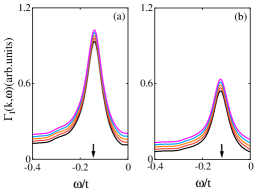
Figure 5: (Color online) The dressed quasiparticle scattering rate at (a) the antinode and (b) the node as a function of energy in $\delta=0.15$ with $T=0.002J$ for the impurity concentrations $n_{i}=0$ (black-line), $0.0025$ (red-line), $0.005$ (orange-line), $0.0075$ (blue-line), and $0.01$ (magenta-line), where the red arrows indicate the positions of the peaks.

To see this picture more clearly, we plot $\Gamma_{\rm I}({\bf k},\omega)$ as a function of energy at (a) the antinode and (b) the node in $\delta=0.15$ with $T=0.002J$ for the impurity concentrations $n_{i}=0$ (black line), $0.0025$ (red line), $0.005$ (orange line), $0.0075$ (blue line), and $0.01$ (magenta line) in Fig. 5. It thus shows clearly that as the case in the pure system Gao18a , the peak structure also appears at around the antinodal and nodal regions in the presence of the impurity scattering, where $\Gamma_{\rm I}({\bf k},\omega)$ achieves a sharp peak at the peak energy, and then it decreases rapidly away from this peak energy DMou17 . More importantly, the position of this sharp peak is just corresponding to the position of the dip in the PDH structure in the dressed quasiparticle excitation spectrum shown in Fig. 4. In this case, the spectral weight at around the dip energy is suppressed heavily by the strong quasiparticle scattering, and then the PDH structure is developed at around the antinodal and nodal regions DMou17 . On the other hand, the impurity scattering self-energy in the particle-hole channel further enhances the quasiparticle scattering as shown in Fig. 5, which therefore leads to a further depression of the spectral weights of the coherent peak at the low binding-energy and the hump at the higher binding-energy Vobornik99 ; Vobornik00 ; Shen04 ; Kondo07 ; Pan09 . However, the impurity scattering self-energy in the particle-particle channel induces a strong deviation from the d-wave behaviour of the SC gap (then an existence of a finite gap over the entire EFS) Shen04 ; Kondo07 ; Pan09 with the exotic impurity concentration dependence of the gap behaviours at around the nodal and antinodal regions Vobornik99 ; Vobornik00 as we have mentioned in subsection III.1, which thus leads to that with the increase of the impurity concentration, the position of the low binding-energy coherent peak at around the antinodal region is shifted smoothly towards to EFS, while the position of the low binding-energy coherent peak at around the nodal region progressively moves away from EFS.

III.3 ARPES autocorrelation

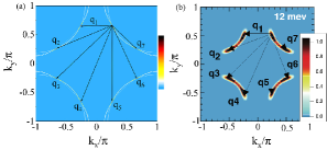
Figure 6: (Color online) (a) The intensity map of the quasiparticle excitation spectrum in the binding-energy $\omega=12$ meV at $\delta=0.15$ with $T=0.002J$ for the impurity concentration $n_{i}=0.0005$. (b) The corresponding experimental result of the optimally doped Bi₂Sr₂CaCu₂O_8+δ for $\omega=12$ meV taken from Ref. Chatterjee06, . ${\bf q}_{1}$, ${\bf q}_{2}$, ${\bf q}_{3}$, ${\bf q}_{4}$, ${\bf q}_{5}$, ${\bf q}_{6}$, and ${\bf q}_{7}$ indicate different scattering wave vectors.

We now turn to discuss the ARPES autocorrelation of cuprate superconductors for a further understanding of the nature of the quasiparticle excitation. Experimentally, ARPES probes directly the momentum-space electronic structure of the system Damascelli03 ; Campuzano04 ; Fink07 , while the ARPES autocorrelation detects directly the effectively momentum-resolved joint density of states in the electronic state Chatterjee06 ; He14 , yielding the important insights into the nature of the quasiparticle excitation. On the other hand, scanning tunneling spectroscopy (STS) observes directly the real-space inhomogeneous electronic structure of the system Yin21 . In particular, this STS technique has been also used to infer the momentum-space behavior of the quasiparticle excitations of cuprate superconductors from the Fourier transform (FT) of the position- and energy-dependent local density of states (LDOS) $\rho({\bf r},\omega)$, and then both the real- and momentum-spaces modulations for LDOS are explored simultaneously Yin21 ; Pan01 ; Hoffman02 ; Kohsaka07 ; Kohsaka08 ; Hamidian16 . The characteristic feature observed by the FT-STS LDOS $\rho({\bf q},\omega)$ is some sharp peaks at the well-defined wave vectors ${\bf q}_{i}$ obeying the octet model as shown in Fig. 1, the quasiparticle scattering interference (QSI) Yin21 ; Pan01 ; Hoffman02 ; Kohsaka07 ; Kohsaka08 ; Hamidian16 then manifests itself as a spatial modulation of $\rho({\bf r},\omega)$ with these well-defined wave vector ${\bf q}_{i}$, appearing in the FT-STS LDOS $\rho({\bf q},\omega)$. More importantly, it has been demonstrated experimentally Chatterjee06 ; He14 that the sharp peaks in the ARPES autocorrelation spectrum are directly correlated with the quasiparticle scattering wave vectors ${\bf q}_{i}$ connecting the tips of the Fermi arcs in the octet scattering model as shown in Fig. 1, and are also well consistent with the QSI peaks observed from the FT-STS experiments Yin21 ; Pan01 ; Hoffman02 ; Kohsaka07 ; Kohsaka08 ; Hamidian16 . This is also why the main features of QSI observed in the FT-STS experiments Yin21 ; Pan01 ; Hoffman02 ; Kohsaka07 ; Kohsaka08 ; Hamidian16 can be also detected from the ARPES autocorrelation experiments Chatterjee06 ; He14 . In this subsection, we further discuss the influence of the impurity scattering on the electronic state in terms of the autocorrelation of the quasiparticle excitation spectra.

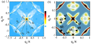
Figure 7: (Color online) (a) The intensity map of the autocorrelation spectrum in the binding-energy $\omega=12$ meV at $\delta=0.15$ with $T=0.002J$ for the impurity concentration $n_{i}=0.0005$. (b) The corresponding experimental result of the ARPES autocorrelation spectrum observed from the optimally doped Bi₂Sr₂CaCu₂O_8+δ for the binding-energy $\omega=12$ meV taken from Ref. Chatterjee06, .

The ARPES autocorrelation of cuprate superconductors is described in terms of the quasiparticle excitation spectrum in Eq. (48) as Chatterjee06 ,

$${\bar{C}}_{\rm I}({\bf q},\omega)={1\over N}\sum_{\bf k}I_{\rm I}({\bf k}+{\bf q},\omega)I_{\rm I}({\bf k},\omega),$$ (51)

which measures the autocorrelation of the quasiparticle excitation spectra in Eq. (48) at two different momenta ${\bf k}$ and ${\bf k}+{\bf q}$, where the summation of momentum ${\bf k}$ is restricted within the first BZ just as it has been done in the experiments Chatterjee06 . In subsection II.2, the topology of EFS (then the zero energy contour) in the pure system has been discussed, where the tips of the Fermi arcs connected by the scattering wave vectors ${\bf q}_{i}$ construct an octet scattering model shown in Fig. 1. More specifically, this octet scattering model shown in Fig. 1 can persist into the system in the presence of impurities at the case for a finite binding-energy Chatterjee06 . To see this important feature more clearly, we plot an intensity map of the dressed quasiparticle excitation spectrum $I_{\rm I}({\bf k},\omega)$ in the case of the binding-energy $\omega=12$ meV at $\delta=0.15$ with $T=0.002J$ for the impurity concentration $n_{i}=0.0005$ in Fig. 6a. For a clear comparison, the corresponding ARPES experimental result Chatterjee06 observed on the optimally doped Bi₂Sr₂CaCu₂O_8+δ for the case of the binding-energy $\omega=12$ meV is also shown in Fig. 6b. It thus shows that the octet scattering model with the scattering wave vectors ${\bf q}_{i}$ connecting the tips of the Fermi arcs emerges in the system in the presence of impurities at the case for a finite binding-energy, which is well consistent with the corresponding ARPES experimental result Chatterjee06 .

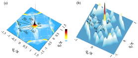
Figure 8: (Color online) (a) The surface plot of the autocorrelation spectrum in the binding-energy $\omega=18$ meV at $\delta=0.15$ with $T=0.002J$ for the impurity concentration $n_{i}=0.0005$. (b) The corresponding experimental result of the ARPES autocorrelation observed from the optimally doped Bi₂Sr₂CaCu₂O_8+δ for the binding-energy $\omega=18$ meV taken from Ref. Chatterjee06, .

We are now ready to discuss the ARPES autocorrelation in cuprate superconductors. In Fig. 7a, we plot the intensity map of the autocorrelation of the quasiparticle excitation spectra ${\bar{C}}_{\rm I}({\bf q},\omega)$ in the binding-energy $\omega=12$ meV at $\delta=0.15$ with $T=0.002J$ for the impurity concentration $n_{i}=0.0005$. For a better comparison, the corresponding experimental result Chatterjee06 detected from the optimally doped Bi₂Sr₂CaCu₂O_8+δ for the bind-energy $\omega=12$ meV is also shown in Fig. 7b. Obviously, the corresponding ARPES experimental result Chatterjee06 is qualitatively reproduced, where the main features can be summarized as: (i) there are some discrete spots appear in ${\bar{C}}_{\rm I}({\bf q},\omega)$, where the joint density of states is highest; (ii) these discrete spots in ${\bar{C}}_{\rm I}({\bf q},\omega)$ are directly correlated with the corresponding wave vectors ${\bf q}_{i}$ connecting the tips of the Fermi arcs in the octet scattering model shown in Fig. 6; (iii) the momentum-space structure of the ARPES autocorrelation pattern of ${\bar{C}}_{\rm I}({\bf q},\omega)$ is quite similar to the momentum-space structure of the QSI pattern observed from FT-STS experiments Yin21 ; Pan01 ; Hoffman02 ; Kohsaka07 ; Kohsaka08 ; Hamidian16 . To see the autocorrelation pattern of ${\bar{C}}_{\rm I}({\bf q},\omega)$ more clearly, the surface plot of ${\bar{C}}_{\rm I}({\bf q},\omega)$ in the binding-energy $\omega=18$ meV at $\delta=0.15$ with $T=0.002J$ for the impurity concentration $n_{i}=0.0005$ is shown in Fig. 8a in comparison with the corresponding experimental result Chatterjee06 observed on the optimally doped Bi₂Sr₂CaCu₂O_8+δ for the binding-energy $\omega=18$ meV in Fig. 8b, where as was expected, the sharp autocorrelation peaks are located exactly at the discrete spots of ${\bar{C}}_{\rm I}({\bf q},\omega)$.

In addition to the results plotted in the above Fig. 7 and Fig. 8, we have also performed a series of calculations for ${\bar{C}}_{\rm I}({\bf q},\omega)$ with other different sets of the strength of the impurity scattering at different impurity concentrations as in the case of the discussions in Sec. III.1. Comparing these results together with the results shown in Fig. 7 and Fig. 8 with the corresponding results in the pure system Gao19 , we thus find that except for the sharp peaks in the autocorrelation pattern in the pure system that are broadened by the impurity scattering, (i) at a given set of the impurity scattering strength, the weight of the extra peaks in the autocorrelation pattern of the pure system is smoothly depressed when the impurity concentration level is raised, and (ii) on the other hand, at a given impurity concentration, the weight of the extra peaks in the autocorrelation pattern of the pure system is gradually suppressed with the increase of the impurity scattering strength. In other words, the impurity concentration presents a similar behavior of the impurity scattering strength. More importantly, in the reasonable parameter range of the impurity scattering strength and impurity concentration, $45J<V_{1}<95J$, $V_{j}<V_{1}$ with $j=2,3,4,...8$, and $0.0004<n_{i}<0.00055$, the weight of the extra peaks in the autocorrelation pattern of the pure system is eliminated completely by the impurity scattering as the results shown in Fig. 7 and Fig. 8, leading to that the obtained results of the autocorrelation pattern as the results shown in Fig. 7 and Fig. 8 are consistent with the corresponding ARPES experimental observations Chatterjee06 on the optimally doped Bi₂Sr₂CaCu₂O_8+δ. The qualitative agreement between the theoretical results and experimental observations therefore indicate that the unconventional features of the ARPES autocorrelation pattern (then the QSI pattern) are dominated by both the strong electron correlation and impurity scattering. The present study also shows that the microscopic octet scattering model obtained based on the kinetic-energy-driven superconductivity can give a consistent description of the influence of impurities on the electronic structure in cuprate superconductors.

IV Summary and discussions

Starting from the $t$-$J$ model in the fermion-spin representation, we have rederived the homogenous part of the electron propagator with the d-wave symmetry based on the kinetic-energy-driven SC mechanism, and shown that the formation of the Fermi arcs is due to the EFS reconstruction, where a large number of the low-energy electronic states is available at around the tips of the Fermi arcs, and then the most physical properties of cuprate superconductors are controlled by the quasiparticle excitations at around the tips of the Fermi arcs. These tips of the Fermi arcs connected by the scattering wave vectors ${\bf q}_{i}$ naturally construct an octet scattering model. With the help of this homogenous electron propagator and the associated octet scattering model, we then have investigated the influence of the impurity scattering on the electronic structure of cuprate superconductors within the standard perturbation theory, where although the impurity scattering is treated in terms of the self-consistent $T$-matrix approach, the impurity scattering self-energy is evaluated firstly in the Fermi-arc-tip approximation of the quasiparticle excitations and scattering processes. The obtained results show that (i) the quasiparticle band structure is further renormalized by the real part of the impurity scattering self-energy in the particle-hole channel, while the quasiparticle lifetime is further reduced by the corresponding imaginary part of the impurity scattering self-energy, with the renormalization strength and reduction extent that increase as the impurity concentration is increased; (ii) the impurity scattering self-energy in the particle-particle channel generates a strong deviation from the d-wave behaviour of the SC gap, where with the increase of the impurity concentration, the magnitude of the SC gap along EFS is progressively reduced except for at around the nodal region, where the gap that vanishes in the pure system opens with the magnitude of the gap that smoothly increases, which therefore leads to the existence of a finite gap over the entire EFS. Furthermore, we have employed these impurity scattering self-energies in the particle-hole and particle-particle channels to study the influence of the impurity scattering on the complicated line-shape in the quasiparticle excitation spectrum and the ARPES autocorrelation spectrum, and the obtained results are well consistent with the corresponding experimental observations. Our theory therefore indicates that the unconventional features of the electronic structure in cuprate superconductors are generated by both the strong electron correlation and impurity scattering.

The theoretical framework, especially the Fermi-arc-tip approximation, developed in this paper for the understanding of the influence of the impurity scattering on the electronic structure of cuprate superconductors can be also employed to study the influence of the impurity scattering on other various properties of cuprate superconductors both in the SC- and normal-states. In particular, based on this theoretical framework, we have also discussed the energy dependence of the SC-state quasiparticle transport in cuprate superconductors by the consideration of the contributions of the vertex correction Zeng22 . These and the related works will be presented elsewhere.

Appendix A T-matrix equation

In this Appendix, we derive explicitly the result of the T-matrix equation (38) of the main text. The self-consistent T-matrix equation (37) can be expanded in the following way,

$$\tilde{T}_{\mu\nu} = \bar{V}_{\mu\nu}\otimes\tau_{3}$$ (52)

$$+ \bar{V}_{\mu{\rm A}}\otimes[\tau_{3}\tilde{I}^{\rm(A)}_{\tilde{G}}(\omega)]\{\bar{V}_{{\rm A}\nu}\otimes\tau_{3}+\bar{V}_{\rm AA}\otimes[\tau_{3}\tilde{I}^{\rm(A)}_{\tilde{G}}(\omega)](\bar{V}_{{\rm A}\nu}\otimes\tau_{3}+\bar{V}_{\rm AA}\otimes[\tau_{3}\tilde{I}^{\rm(A)}_{\tilde{G}}(\omega)]\tilde{T}_{{\rm A}\nu}+\bar{V}_{\rm AB}\otimes[\tau_{3}\tilde{I}^{\rm(B)}_{\tilde{G}}(\omega)]\tilde{T}_{{\rm B}\nu})$$

$$+ \bar{V}^{\rm AB}\otimes[\tau_{3}\tilde{I}^{\rm(B)}_{\tilde{G}}(\omega)](\bar{V}_{{\rm B}\nu}\otimes\tau_{3}+\bar{V}_{\rm BA}\otimes[\tau_{3}\tilde{I}^{\rm(A)}_{\tilde{G}}(\omega)]*\tilde{T}_{{\rm A}\nu}+\bar{V}_{\rm BB}\otimes[\tau_{3}\tilde{I}^{\rm(B)}_{\tilde{G}}(\omega)]*\tilde{T}_{{\rm B}\nu})\}$$

$$+ \bar{V}_{\mu{\rm B}}\otimes[\tau_{3}\tilde{I}^{\rm(B)}_{\tilde{G}}(\omega)]\{\bar{V}_{{\rm B}\nu}\otimes\tau_{3}+\bar{V}_{\rm BA}\otimes[\tau_{3}\tilde{I}^{\rm(A)}_{\tilde{G}}(\omega)](\bar{V}_{{\rm A}\nu}\otimes\tau_{3}+\bar{V}_{\rm AA}\otimes[\tau_{3}\tilde{I}^{\rm(A)}_{\tilde{G}}(\omega)]\tilde{T}_{{\rm A}\nu}+\bar{V}_{\rm AB}\otimes[\tau_{3}\tilde{I}^{\rm(B)}_{\tilde{G}}(\omega)]\tilde{T}_{{\rm B}\nu})$$

$$+ \bar{V}_{\rm BB}\otimes[\tau_{3}\tilde{I}^{\rm(B)}_{\tilde{G}}(\omega)](\bar{V}_{{\rm B}\nu}\otimes\tau_{3}+\bar{V}_{\rm BA}\otimes[\tau_{3}\tilde{I}^{\rm(A)}_{\tilde{G}}(\omega)]\tilde{T}_{{\rm A}\nu}+\bar{V}_{\rm BB}\otimes[\tau_{3}\tilde{I}^{\rm(B)}_{\tilde{G}}(\omega)]\tilde{T}_{{\rm B}\nu})\}$$

$$= \bar{V}_{\mu\nu}\otimes\tau_{3}+\bar{V}_{\mu{\rm A}}\bar{V}_{{\rm A}\nu}\otimes[\tau_{3}\tilde{I}^{\rm(A)}_{\tilde{G}}(\omega)]\tau_{3}+\bar{V}_{\mu{\rm B}}\bar{V}_{{\rm B}\nu}\otimes[\tau_{3}\tilde{I}^{\rm(B)}_{\tilde{G}}(\omega)]\tau_{3}$$

$$+ \bar{V}_{\mu{\rm A}}\bar{V}_{\rm AA}\bar{V}_{{\rm A}\nu}\otimes[\tau_{3}\tilde{I}^{\rm(A)}_{\tilde{G}}(\omega)]^{2}\tau_{3}+\bar{V}_{\mu{\rm A}}\bar{V}_{\rm AB}\bar{V}_{{\rm B}\nu}\otimes[\tau_{3}\tilde{I}^{\rm(A)}_{\tilde{G}}(\omega)][\tau_{3}\tilde{I}^{\rm(B)}_{\tilde{G}}(\omega)]\tau_{3}$$

$$+ \bar{V}_{\mu{\rm B}}\bar{V}_{\rm BA}\bar{V}_{{\rm A}\nu}\otimes[\tau_{3}\tilde{I}^{\rm(B)}_{\tilde{G}}(\omega)][\tau_{3}\tilde{I}^{\rm(A)}_{\tilde{G}}(\omega)]\tau_{3}+\bar{V}_{\mu{\rm B}}\bar{V}_{\rm BB}\bar{V}_{{\rm B}\nu}\otimes[\tau_{3}\tilde{I}^{\rm(B)}_{\tilde{G}}(\omega)]^{2}\tau_{3}$$

$$+ \bar{V}_{\mu{\rm A}}\bar{V}_{\rm AA}\bar{V}_{\rm AA}\otimes[\tau_{3}\tilde{I}^{\rm(A)}_{\tilde{G}}(\omega)]^{3}\tilde{T}_{{\rm A}\nu}+\bar{V}_{\mu{\rm A}}\bar{V}_{\rm AA}\bar{V}_{\rm AB}\otimes[\tau_{3}\tilde{I}^{\rm(A)}_{\tilde{G}}(\omega)]^{2}[\tau_{3}\tilde{I}^{\rm(B)}_{\tilde{G}}(\omega)]\tilde{T}_{{\rm B}\nu}$$

$$+ \bar{V}_{\mu{\rm A}}\bar{V}_{\rm AB}\bar{V}_{\rm BA}\otimes[\tau_{3}\tilde{I}^{\rm(A)}_{\tilde{G}}(\omega)][\tau_{3}\tilde{I}^{\rm(B)}_{\tilde{G}}(\omega)][\tau_{3}\tilde{I}^{\rm(A)}_{\tilde{G}}(\omega)]\tilde{T}_{{\rm A}\nu}+\bar{V}_{\mu{\rm A}}\bar{V}_{\rm AB}\bar{V}_{\rm BB}\otimes[\tau_{3}\tilde{I}^{\rm(A)}_{\tilde{G}}(\omega)][\tau_{3}\tilde{I}^{\rm(B)}_{\tilde{G}}(\omega)]^{2}\tilde{T}_{{\rm B}\nu}$$

$$+ \bar{V}_{\mu{\rm B}}\bar{V}_{\rm BA}\bar{V}_{\rm AA}\otimes[\tau_{3}\tilde{I}^{\rm(B)}_{\tilde{G}}(\omega)][\tau_{3}\tilde{I}^{\rm(A)}_{\tilde{G}}(\omega)]^{2}*\tilde{T}_{{\rm A}\nu}+\bar{V}_{\mu{\rm B}}\bar{V}_{\rm BA}\bar{V}_{\rm AB}\otimes[\tau_{3}\tilde{I}^{\rm(B)}_{\tilde{G}}(\omega)][\tau_{3}\tilde{I}^{\rm(A)}_{\tilde{G}}(\omega)][\tau_{3}\tilde{I}^{\rm(B)}_{\tilde{G}}(\omega)]\tilde{T}_{{\rm B}\nu}$$

$$+ \bar{V}_{\mu{\rm B}}\bar{V}_{\rm BB}\bar{V}_{\rm BA}\otimes[\tau_{3}\tilde{I}^{\rm(B)}_{\tilde{G}}(\omega)]^{2}[\tau_{3}\tilde{I}^{\rm(A)}_{\tilde{G}}(\omega)]\tilde{T}_{{\rm A}\nu}+\bar{V}_{\mu{\rm B}}\bar{V}_{\rm BB}\bar{V}_{\rm BB}\otimes[\tau_{3}\tilde{I}^{\rm(B)}_{\tilde{G}}(\omega)]^{3}\tilde{T}_{{\rm B}\nu}.$$

To solve this self-consistent T-matrix equation, we define a $4\times 4$ unit matrix $\hat{I}_{\upsilon}$ in the $\bar{V}$-space, and then right multiply the matrix $\hat{I}_{\upsilon}\otimes\tau_{3}$ in the above T-matrix equation (52), which leads to an iterative T-matrix equation as,

$$\tilde{T}_{\mu\nu}*\hat{I}_{\upsilon}\otimes\tau_{3} = \sum\limits_{\alpha}T^{(\alpha)}_{\mu\nu}\otimes\tau_{\alpha}\tau_{3}$$ (53)

$$= \bar{V}_{\mu\nu}\otimes\tau_{0}+\bar{V}_{\mu{\rm A}}\bar{V}_{{\rm A}\nu}\otimes[\tau_{3}\tilde{I}^{\rm(A)}_{\tilde{G}}(\omega)]+\bar{V}_{\mu{\rm B}}\bar{V}_{{\rm B}\nu}\otimes[\tau_{3}\tilde{I}^{\rm(B)}_{\tilde{G}}(\omega)]+\bar{V}_{\mu{\rm A}}\bar{V}_{{\rm AA}}\bar{V}_{{\rm A}\nu}\otimes[\tau_{3}\tilde{I}^{\rm(A)}_{\tilde{G}}(\omega)]^{2}$$

$$+ \bar{V}_{\mu{\rm A}}\bar{V}_{\rm AB}\bar{V}_{{\rm B}\nu}\otimes[\tau_{3}\tilde{I}^{\rm(A)}_{\tilde{G}}(\omega)][\tau_{3}\tilde{I}^{\rm(B)}_{\tilde{G}}(\omega)]+\bar{V}_{\mu{\rm B}}\bar{V}_{\rm BA}\bar{V}_{{\rm A}\nu}\otimes[\tau_{3}\tilde{I}^{\rm(B)}_{\tilde{G}}(\omega)][\tau_{3}\tilde{I}^{\rm(A)}_{\tilde{G}}(\omega)]+\bar{V}_{\mu{\rm B}}\bar{V}_{\rm BB}\bar{V}_{{\rm B}\nu}\otimes[\tau_{3}\tilde{I}^{\rm(B)}_{\tilde{G}}(\omega)]^{2}$$

$$+ \bar{V}_{\mu{\rm A}}\bar{V}_{\rm AA}\bar{V}_{\rm AA}\otimes[\tau_{3}\tilde{I}^{\rm(A)}_{\tilde{G}}(\omega)]^{3}\sum\limits_{\alpha}T^{(\alpha)}_{{\rm A}\nu}\otimes\tau_{\alpha}\tau_{3}+\bar{V}_{\mu{\rm A}}\bar{V}_{\rm AA}\bar{V}_{\rm AB}\otimes[\tau_{3}\tilde{I}^{\rm(A)}_{\tilde{G}}(\omega)]^{2}[\tau_{3}\tilde{I}^{\rm(B)}_{\tilde{G}}(\omega)]\sum\limits_{\alpha}T^{(\alpha)}_{{\rm B}\nu}\otimes\tau_{\alpha}\tau_{3}$$

$$+ \bar{V}_{\mu{\rm A}}\bar{V}_{\rm AB}\bar{V}_{\rm BA}\otimes[\tau_{3}\tilde{I}^{\rm(A)}_{\tilde{G}}(\omega)][\tau_{3}\tilde{I}^{\rm(B)}_{\tilde{G}}(\omega)][\tau_{3}\tilde{I}^{\rm(A)}_{\tilde{G}}(\omega)]\sum\limits_{\alpha}T^{(\alpha)}_{{\rm A}\nu}\otimes\tau_{\alpha}\tau_{3}$$

$$+ \bar{V}_{\mu{\rm A}}\bar{V}_{\rm AB}\bar{V}_{\rm BB}\otimes[\tau_{3}\tilde{I}^{\rm(A)}_{\tilde{G}}(\omega)][\tau_{3}\tilde{I}^{\rm(B)}_{\tilde{G}}(\omega)]^{2}\sum\limits_{\alpha}T^{(\alpha)}_{{\rm B}\nu}\otimes\tau_{\alpha}\tau_{3}$$

$$+ \bar{V}_{\mu{\rm B}}\bar{V}_{\rm BA}\bar{V}{\rm AA}\otimes[\tau_{3}\tilde{I}^{\rm(B)}_{\tilde{G}}(\omega)][\tau_{3}\tilde{I}^{\rm(A)}_{\tilde{G}}(\omega)]^{2}\sum\limits_{\alpha}T^{(\alpha)}_{{\rm A}\nu}\otimes\tau_{\alpha}\tau_{3}$$

$$+ \bar{V}_{\mu{\rm B}}\bar{V}_{\rm BA}\bar{V}_{\rm AB}\otimes[\tau_{3}\tilde{I}^{\rm(B)}_{\tilde{G}}(\omega)][\tau_{3}\tilde{I}^{\rm(A)}_{\tilde{G}}(\omega)][\tau_{3}\tilde{I}^{\rm(B)}_{\tilde{G}}(\omega)]\sum\limits_{\alpha}T^{(\alpha)}_{{\rm B}\nu}\otimes\tau_{\alpha}\tau_{3}$$

$$+ \bar{V}_{\mu{\rm B}}\bar{V}_{\rm BB}\bar{V}_{\rm BA}\otimes[\tau_{3}\tilde{I}^{\rm(B)}_{\tilde{G}}(\omega)]^{2}[\tau_{3}\tilde{I}^{\rm(A)}_{\tilde{G}}(\omega)]\sum\limits_{\alpha}T^{(\alpha)}_{{\rm A}\nu}\otimes\tau_{\alpha}\tau_{3}$$

$$+ \bar{V}_{\mu{\rm B}}\bar{V}_{\rm BB}\bar{V}_{\rm BB}\otimes[\tau_{3}\tilde{I}^{\rm(B)}_{\tilde{G}}(\omega)]^{3}\sum\limits_{\alpha}T^{(\alpha)}_{{\rm B}\nu}\otimes\tau_{\alpha}\tau_{3}.$$

Now it is quite easy to verify that the above T-matrix satisfies the following equation,

$$\sum\limits_{\alpha}T^{(\alpha)}_{\mu\nu}\otimes\tau_{\alpha}\tau_{3} = [\bar{V}\otimes\tau_{0}(1+\tilde{M}+\tilde{M}^{2}+\tilde{M}^{3}+\cdots)]_{\mu\nu}=\left(\bar{V}\otimes\tau_{0}{1\over 1-\tilde{M}}\right)_{\mu\nu}$$ (56)

$$= \left[\left(\begin{array}[]{cc}\bar{V}_{\rm AA}\otimes\tau_{0},&\bar{V}_{\rm AB}\otimes\tau_{0}\\ \bar{V}_{\rm BA}\otimes\tau_{0},&\bar{V}_{\rm BB}\otimes\tau_{0}\end{array}\right){1\over 1-\tilde{M}}\right]_{\mu\nu},$$

where the matrix $\tilde{M}$ has been given in Eq. (42) of the main text. Following the Einstein summation rule, the inverse matrix $\bar{M}=(1-\tilde{M})^{-1}$ can be expressed as,

$$\bar{M}=\Lambda^{(\alpha)}\otimes\tau_{\alpha}=\left(\begin{array}[]{ccc}\Lambda_{\rm AA}^{(\alpha)}\otimes\tau_{\alpha}&\vline&\Lambda_{\rm AB}^{(\alpha)}\otimes\tau_{\alpha}\\ \hline\cr\Lambda_{\rm BA}^{(\alpha)}\otimes\tau_{\alpha}&\vline&\Lambda_{\rm BB}^{(\alpha)}\otimes\tau_{\alpha}\end{array}\right)=\left(\begin{array}[]{ccccccccc}\Lambda_{11}^{(\alpha)}\tau_{\alpha}&\Lambda_{12}^{(\alpha)}\tau_{\alpha}&\cdots&\Lambda_{14}^{(\alpha)}\tau_{\alpha}&\vline&\Lambda_{15}^{(\alpha)}\tau_{\alpha}&\Lambda_{16}^{(\alpha)}\tau_{\alpha}&\cdots&\Lambda_{18}^{(\alpha)}\tau_{\alpha}\\ \Lambda_{21}^{(\alpha)}\tau_{\alpha}&\Lambda_{22}^{(\alpha)}\tau_{\alpha}&\cdots&\Lambda_{24}^{(\alpha)}\tau_{\alpha}&\vline&\Lambda_{25}^{(\alpha)}\tau_{\alpha}&\Lambda_{26}^{(\alpha)}\tau_{\alpha}&\cdots&\Lambda_{28}^{(\alpha)}\tau_{\alpha}\\ \vdots&\vdots&\vdots&\vdots&\vline&\vdots&\vdots&\vdots&\vdots\\ \Lambda_{41}^{(\alpha)}\tau_{\alpha}&\Lambda_{42}^{(\alpha)}\tau_{\alpha}&\cdots&\Lambda_{44}^{(\alpha)}\tau_{\alpha}&\vline&\Lambda_{45}^{(\alpha)}\tau_{\alpha}&\Lambda_{46}^{(\alpha)}\tau_{\alpha}&\cdots&\Lambda_{48}^{(\alpha)}\tau_{\alpha}\\ \hline\cr\Lambda_{51}^{(\alpha)}\tau_{\alpha}&\Lambda_{52}^{(\alpha)}\tau_{\alpha}&\cdots&\Lambda_{54}^{(\alpha)}\tau_{\alpha}&\vline&\Lambda_{55}^{(\alpha)}\tau_{\lambda}&\Lambda_{56}^{(\alpha)}\tau_{\alpha}&\cdots&\Lambda_{58}^{(\alpha)}\tau_{\alpha}\\ \Lambda_{61}^{(\alpha)}\tau_{\alpha}&\Lambda_{62}^{(\alpha)}\tau_{\alpha}&\cdots&\Lambda_{64}^{(\alpha)}\tau_{\alpha}&\vline&\Lambda_{65}^{(\alpha)}\tau_{\alpha}&\Lambda_{66}^{(\alpha)}\tau_{\lambda}&\cdots&\Lambda_{68}^{(\alpha)}\tau_{\lambda}\\ \vdots&\vdots&\vdots&\vdots&\vline&\vdots&\vdots&\vdots&\vdots\\ \Lambda_{81}^{(\alpha)}\tau_{\lambda}&\Lambda_{82}^{(\alpha)}\tau_{\alpha}&\cdots&\Lambda_{84}^{(\alpha)}\tau_{\alpha}&\vline&\Lambda_{85}^{(\alpha)}\tau_{\alpha}&\Lambda_{86}^{(\alpha)}\tau_{\alpha}&\cdots&\Lambda_{88}^{(\alpha)}\tau_{\alpha}\\ \end{array}\right).~{}~{}~{}~{}$$ (67)

However, according to the Pauli matrixes $\tau_{0}$, $\tau_{1}$, $\tau_{2}$, and $\tau_{3}$, the block $[jj^{\prime}]$ of the matrix $\bar{M}$ can be decomposed as,

$$\bar{M}_{jj^{\prime}}=\sum\limits_{\alpha=0}^{3}\Lambda_{jj^{\prime}}^{(\alpha)}\tau_{\alpha} = {1\over 2}(\bar{M}_{jj^{\prime}}+\bar{M}_{j+1j^{\prime}+1})\tau_{0}+{1\over 2}(\bar{M}_{jj^{\prime}}-\bar{M}_{j+1j^{\prime}+1})\tau_{3}$$ (68)

$$+ {1\over 2}(\bar{M}_{jj^{\prime}+1}+\bar{M}_{j+1j^{\prime}})\tau_{1}+{i\over 2}(\bar{M}_{jj^{\prime}+1}-\bar{M}_{j+1j^{\prime}})\tau_{2},$$

and then the final form of the T-matrix in Eq. (56) can be obtained as,

$$\sum\limits_{\alpha}T^{(\alpha)}_{\mu\nu}\otimes\tau_{\alpha}\tau_{3} = \left[\left(\begin{array}[]{ccc}\bar{V}_{\rm AA}\otimes\tau_{0}&\vline&\bar{V}_{\rm AB}\otimes\tau_{0}\\ \hline\cr\bar{V}_{\rm BA}\otimes\tau_{0}&\vline&\bar{V}_{\rm BB}\otimes\tau_{0}\end{array}\right)\left(\begin{array}[]{ccc}\Lambda_{\rm AA}^{(\alpha)}\otimes\tau_{\alpha}&\vline&\Lambda_{\rm AB}^{(\alpha)}\otimes\tau_{\alpha}\\ \hline\cr\Lambda_{\rm BA}^{(\alpha)}\otimes\tau_{\alpha}&\vline&\Lambda_{\rm BB}^{(\alpha)}\otimes\tau_{\alpha}\end{array}\right)\right]_{\mu\nu}$$ (73)

$$= \sum\limits_{\mu^{\prime}={\rm A}}^{\rm B}\sum\limits_{\alpha=0}^{3}\bar{V}_{\mu\mu^{\prime}}\Lambda^{(\alpha)}_{\mu^{\prime}\nu}\otimes\tau_{\alpha}=\sum\limits_{\alpha=0}^{3}(\sum\limits_{\mu^{\prime}={\rm A}}^{\rm B}\bar{V}_{\mu\mu^{\prime}}\Lambda^{(\alpha)}_{\mu^{\prime}\nu})\otimes\tau_{\alpha},$$ (74)

which is the same as quoted in Eq. (38) of the main text.

References

- (1) J. G. Bednorz and K. A. Müller, Z. Phys. B 64, 189 (1986).
- (2) M. K. Wu, J. R. Ashburn, C. J. Torng, P. H. Hor, R. L. Meng, L. Gao, Z. J. Huang, Y. Q. Wang, and C. W. Chu, Phys. Rev. Lett. 58, 908 (1987).
- (3) See, e.g., the review, M. Fujita, H. Hiraka, M. Matsuda, M. Matsuura, J. M. Tranquada, S. Wakimoto, G. Xu, and K. Yamada, J. Phys. Soc. Jpn. 81, 011007 (2012).
- (4) See, e.g., the review, N. E. Hussey, Adv. Phys. 51, 1685 (2002), and references therein.
- (5) See, e.g., the review, A. V. Balatsky, I. Vekhter, and J.-X. Zhu, Rev. Mod. Phys. 78, 373 (2006), and references therein.
- (6) See, e.g., the review, H. Alloul, J. Bobroff, M. Gabay, and P. J. Hirschfeld, Rev. Mod. Phys. 81, 45 (2009), and references therein.
- (7) See, e.g., the review, A. Damascelli, Z. Hussain, and Z.-X. Shen, Rev. Mod. Phys. 75, 473 (2003).
- (8) See, e.g., the review, J. C. Campuzano, M. R. Norman, M. Randeira, in Physics of Superconductors, vol. II, edited by K. H. Bennemann and J. B. Ketterson (Springer, Berlin Heidelberg New York, 2004), p. 167.
- (9) See, e.g., the review, J. Fink, S. Borisenko, A. Kordyuk, A. Koitzsch, J. Geck, V. Zabalotnyy, M. Knupfer, B. Buechner, and H. Berger, in Lecture Notes in Physics, vol. 715, edited by S. Hüfner (Springer-Verlag Berlin Heidelberg, 2007), p. 295.
- (10) K. Ishida, Y. Kitaoka, T. Yoshitomi, N. Ogata, T. Kamino, and K. Asayama, Physica C 179, 29 (1991).
- (11) A. Legris, F. Rullier-Albenque, E. Radeva, and P. Lejay, J. Phys. I 3, 1605 (1993).
- (12) J. Giapintzakis, D. M. Ginsberg, M. A. Kirk, and S. Ockers, Phys. Rev. B 50, 15967 (1994).
- (13) Y. Fukuzumi, K. Mizuhashi, K. Takenaka, and S. Uchida, Phys. Rev. Lett. 76, 684 (1996).
- (14) J. P. Attfield, A. L. Kharlanov, and J. A. McAllister, Nature 394, 157 (1998).
- (15) J. Bobroff, W. A. MacFarlane, H. Alloul, P. Mendels, N. Blanchard, G. Collin, and J.-F. Marucco, Phys. Rev. Lett. 83, 4381 (1999).
- (16) H. Eisaki, N. Kaneko, D. L. Feng, A. Damascelli, P. K. Mang, K. M. Shen, Z.-X. Shen, and M. Greven, Phys. Rev. B 69, 064512 (2004).
- (17) I. Vobornik, H. Berger, D. Pavuna, M. Onellion, G. Margaritondo, F. Rullier-Albenque, L. Forró, and M. Grioni, Phys. Rev. Lett. 82, 3128 (1999).
- (18) I. Vobornik, H. Berger, M. Grioni, G. Margaritondo, L. Forró, and F. Rullier-Albenque, Phys. Rev. B 61, 11248 (2000).
- (19) K. M. Shen, T. Yoshida, D. H. Lu, F. Ronning, N. P. Armitage, W. S. Lee, X. J. Zhou, A. Damascelli, D. L. Feng, N. J. C. Ingle, H. Eisaki, Y. Kohsaka, H. Takagi, T. Kakeshita, S. Uchida, P. K. Mang, M. Greven, Y. Onose, Y. Taguchi, Y. Tokura, Seiki Komiya, Yoichi Ando, M. Azuma, M. Takano, A. Fujimori, and Z.-X. Shen, Phys. Rev. B 69, 054503 (2004).
- (20) T. Kondo, T. Takeuchi, A. Kaminski, S. Tsuda, and S. Shin, Phys. Rev. Lett. 98, 267004 (2007).
- (21) Z.-H. Pan, P. Richard, Y.-M. Xu, M. Neupane, P. Bishay, A. V. Fedorov, H. Luo, L. Fang, H.-H. Wen, Z. Wang, and H. Ding, Phys. Rev. B 79, 092507 (2009).
- (22) D. A. Bonn, S. Kamal, K. Zhang, R. Liang, D. J. Baar, E. Klein, and W. N. Hardy, Phys. Rev. B 50, 4051 (1994).
- (23) C. Bucci, P. Carretta, R. D. Renzi, G. Guidia, F. Licci, L. G. Raflob, H. Keller, S. Lee, I. M. Savićc, Physica C 235-240, 1849 (1994).
- (24) C. Bernhard, J. L. Tallon, C. Bucci, R. DeRenzi, G. Guidi, G. V. M. Williams, and C. Niedermayer, Phys. Rev. Lett. 77, 2304 (1996).
- (25) J. Bobroff, Ann. Phys. (Paris) 30, 1 (2005).
- (26) See, e.g., G. D. Mahan, Many-Particle Physics, (Plenum Press, New York, 1981).
- (27) P. J. Hirschfeld, P. Wölfle, J. A. Sauls, D. Einzel, and W. O. Putikka, Phys. Rev. B 40, 6695 (1989).
- (28) P. J. Hirschfeld and N. Goldenfeld, Phys. Rev. B 48, 4219 (1993)
- (29) A. C. Durst and P. A. Lee, Phys. Rev. B 62, 1270 (2000).
- (30) A. G. Yashenkin, W. A. Atkinson, I. V. Gornyi, P. J. Hirschfeld, and D. V. Khveshchenko, Phys. Rev. Lett. 86, 5982 (2001).
- (31) T. S. Nunner and P. J. Hirschfeld, Phys. Rev. B 72, 014514 (2005).
- (32) T. Dahm, P. J. Hirschfeld, D. J. Scalapino, and L. Zhu, Phys. Rev. B 72, 214512 (2005).
- (33) Z. Wang, H. Guo, and S. Feng, Physica C 468, 1078 (2008); Z. Wang and S. Feng, Phys. Rev. B 80, 174507 (2009).
- (34) B. M. Andersen and P. J. Hirschfeld, Phys. Rev. Lett. 100, 257003 (2008)
- (35) Z. Wang and S. Feng, Phys. Rev. B 80, 064510 (2009).
- (36) N. R. Lee-Hone, J. S. Dodge, and D. M. Broun, Phys. Rev. B 96, 024501 (2017); N. R. Lee-Hone, V. Mishra, D. M. Broun, and P. J. Hirschfeld, Phys. Rev. B 98, 054506 (2018).
- (37) U. Chatterjee, M. Shi, A. Kaminski, A. Kanigel, H. M. Fretwell, K. Terashima, T. Takahashi, S. Rosenkranz, Z. Z. Li, H. Raffy, A. Santander-Syro, K. Kadowaki, M. R. Norman, M. Randeria, and J. C. Campuzano, Phys. Rev. Lett. 96, 107006 (2006).
- (38) Y. He, Y. Yin, M. Zech, A. Soumyanarayanan, M. M. Yee, T. Williams, M. C. Boyer, K. Chatterjee, W. D. Wise, I. Zeljkovic, T. Kondo, T. Takeuchi, H. Ikuta, P. Mistark, R. S. Markiewicz, A. Bansil, S. Sachdev, E. W. Hudson, and J. E. Hoffman, Science 344, 608 (2014).
- (39) M. Shi, J. Chang, S. Pailhés, M. R. Norman, J. C. Campuzano, M. Mánsson, T. Claesson, O. Tjernberg, A. Bendounan, L. Patthey, N. Momono, M. Oda, M. Ido, C. Mudry, and J. Mesot, Phys. Rev. Lett. 101, 047002 (2008).
- (40) Y. Sassa, M. Radović, M. Mánsson, E. Razzoli, X. Y. Cui, S. Pailhés, S. Guerrero, M. Shi, P. R. Willmott, F. Miletto Granozio, J. Mesot, M. R. Norman, and L. Patthey, Phys. Rev. B 83, 140511(R) (2011).
- (41) R. Comin, A. Frano, M. M. Yee, Y. Yoshida, H. Eisaki, E. Schierle, E. Weschke, R. Sutarto, F. He, A. Soumyanarayanan, Yang He, M. L. Tacon, I. S. Elfimov, Jennifer E. Hoffman, G. A. Sawatzky, B. Keimer, and A. Damascelli, Science 343, 390 (2014).
- (42) M. Horio, T. Adachi, Y. Mori, A. Takahashi, T. Yoshida, H. Suzuki, L. C. C. Ambolode II, K. Okazaki, K. Ono, H. Kumigashira, H. Anzai, M. Arita, H. Namatame, M. Taniguchi, D. Ootsuki, K. Sawada, M. Takahashi, T. Mizokawa, Y. Koike, and A. Fujimori, Nat. Commun. 7, 10567 (2016).
- (43) B. Loret, Y. Gallais, M. Cazayous, R. D. Zhong, J. Schneeloch, G. D. Gu, A. Fedorov, T. K. Kim, S. V. Borisenko, and A. Sacuto, Phys. Rev. B 97, 174521 (2018).
- (44) See, e.g., the review, J.-X. Yin, S. H. Pan, and M. Z. Hasan, Nat. Rev. Phys. 3, 249 (2021).
- (45) S. H. Pan, J. P. ÓNeal, R. L. Badzey, C. Chamon, H. Ding, J. R. Engelbrecht, Z. Wang, H. Eisaki, S. Uchida, A. K. Gupta, K.-W. Ng, E. W. Hudson, K. M. Lang, and J. C. Davis, Nature 413, 282 (2001).
- (46) J. E. Hoffman, E. W. Hudson, K. M. Lang, V. Madhavan, H. Eisaki, S. Uchida, and J. C. Davis, Science 295, 466 (2002).
- (47) Y. Kohsaka, C. Taylor, K. Fujita, A. Schmidt, C. Lupien, T. Hanaguri, M. Azuma, M. Takano, H. Eisaki, H. Takagi, S. Uchida, and J. C. Davis, Science 315, 1380 (2007).
- (48) Y. Kohsaka, C. Taylor, P. Wahl, A. Schmidt, J. Lee, K. Fujita, J. W. Alldredge, K. McElroy, J. Lee, H. Eisaki, S. Uchida, D.-H. Lee, and J. C. Davis, Nature 454, 1072 (2008).
- (49) M. H. Hamidian, S. D. Edkins, S. Hyun Joo, A. Kostin, H. Eisaki, S. Uchida, M. J. Lawler, E.-A. Kim, A. P. Mackenzie, K. Fujita, J. Lee, and J. C. S. Davis, Nature 532, 343 (2016).
- (50) S. Feng, Phys. Rev. B 68, 184501 (2003); S. Feng, T. Ma, and H. Guo, Physica C 436, 14 (2006).
- (51) S. Feng, H. Zhao, and Z. Huang, Phys. Rev. B. 85, 054509 (2012); Phys. Rev. B 85, 099902(E) (2012).
- (52) S. Feng, L. Kuang, and H. Zhao, Physica C 517, 5 (2015).
- (53) See, e.g., the review, S. Feng, Y. Lan, H. Zhao, L. Kuang, L. Qin, and X. Ma, Int. J. Mod. Phys. B 29, 1530009 (2015).
- (54) P. W. Anderson, Science 235, 1196 (1987).
- (55) See, e.g., the review, L. Yu, in Recent Progress in Many-Body Theories, edited by T. L. Ainsworth, C. E. Campbell, B. E. Clements, and E. Krotscheck (Plenum, New York, 1992), Vol. 3, p. 157.
- (56) S. Feng, J. B. Wu, Z. B. Su, and L. Yu, Phys. Rev. B 47, 15192 (1993).
- (57) L. Zhang, J. K. Jain, and V. J. Emery, Phys. Rev. B 47, 3368 (1993).
- (58) J. C. LeGuillou and E. Ragoucy, Phys. Rev. B 52, 2403 (1995).
- (59) See, e.g., the review, P. A. Lee, N. Nagaosa, and X. G. Wen, Rev. Mod. Phys. 78, 17 (2006).
- (60) S. Feng, J. Qin, and T. Ma, J. Phys.: Condens. Matter 16, 343 (2004); S. Feng, Z. B. Su, and L. Yu, Phys. Rev. B 49, 2368 (1994).
- (61) G. M. Eliashberg, Sov. Phys. JETP 11, 696 (1960).
- (62) Y. Liu, Y. Lan, and S. Feng, Phys. Rev. B 103, 024525 (2021).
- (63) D. Gao, Y. Liu, H. Zhao, Y. Mou, and S. Feng, Physica C 551, 72 (2018).
- (64) See, e.g., the review, T. Timusk and B. Statt, Rep. Prog. Phys. 62, 61 (1999).
- (65) See, e.g., the review, S. Hüfner, M. A. Hossain, A. Damascelli, and G. A. Sawatzky, Rep. Prog. Phys. 71, 062501 (2008).
- (66) See, e.g., the review, R. Comin and A. Damascelli, Annu. Rev. Condens. Matter Phys. 7, 369 (2016).
- (67) See, e.g., the review, I. M. Vishik, Rep. Prog. Phys. 81, 062501 (2018).
- (68) D. Gao, Y. Mou, and S. Feng, J. Low Temp. Phys. 192, 19 (2018).
- (69) D. Gao, Y. Mou, Y. Liu, S. Tan, and S. Feng, Phil. Mag. 99, 752 (2019).
- (70) P. A. Lee, Phys. Rev. Lett. 71, 1887 (1993).
- (71) M. Franz, C. Kallin, and A. J. Berlinsky, Phys. Rev. B 54, R6897 (1996).
- (72) D. S. Dessau, B. O. Wells, Z.-X. Shen, W. E. Spicer, A. J. Arko, R. S. List, D. B. Mitzi, and A. Kapitulnik, Phys. Rev. Lett. 66, 2160 (1991).
- (73) Y. Hwu, L. Lozzi, M. Marsi, S. LaRosa, M. Winokur, P. Davis, M. Onellion, H. Berger, F. Gozzo, F. Lévy, and G. Margaritondo, Phys. Rev. Lett. 67, 2573 (1991).
- (74) M. Randeria, H. Ding, J-C. Campuzano, A. Bellman, G. Jennings, T. Yokoya, T. Takahashi, H. Katayama-Yoshida, T. Mochiku, and K. Kadowaki, Phys. Rev. Lett. 74, 4951 (1995).
- (75) A. V. Fedorov, T. Valla, P. D. Johnson, Q. Li, G. D. Gu, and N. Koshizuka, Phys. Rev. Lett. 82, 2179 (1999).
- (76) D. H. Lu, D. L. Feng, N. P. Armitage, K. M. Shen, A. Damascelli, C. Kim, F. Ronning, Z.-X. Shen, D. A. Bonn, R. Liang, W. N. Hardy, A. I. Rykov, and S. Tajima, Phys. Rev. Lett. 86, 4370 (2001).
- (77) S. Sakai, S. Blanc, M. Civelli, Y. Gallais, M. Cazayous, M.-A. Méasson, J. S. Wen, Z. J. Xu, G. D. Gu, G. Sangiovanni, Y. Motome, K. Held, A. Sacuto, A. Georges, and M. Imada, Phys. Rev. Lett. 111, 107001 (2013).
- (78) B. Loret, S. Sakai, S. Benhabib, Y. Gallais, M. Cazayous, M. A. Méasson, R. D. Zhong, J. Schneeloch, G. D. Gu, A. Forget, D. Colson, I. Paul, M. Civelli, and A. Sacuto, Phys. Rev. B 96, 094525 (2017).
- (79) D. Mou, A. Kaminski, and G. Gu, Phys. Rev. B 95, 174501 (2017).
- (80) M. H. Zeng, X. Li, Y. J. Wang, and S. Feng, unpublished.