Two bands Ising superconductivity from Coulomb interactions in monolayer $\text{NbSe}_{2}$

Abstract

The nature of superconductivity in monolayer transition metal dichalcogenides is still an object of debate. It has already been argued that repulsive Coulomb interactions, combined with the disjoint Fermi surfaces around the $K$, $K^{\prime}$ valleys and at the $\Gamma$ point, can lead to superconducting instabilities in monolayer $\text{NbSe}_{2}$. Here, we demonstrate the two bands nature of superconductivity in $\text{NbSe}_{2}$. It arises from the competition of repulsive long range intravalley and short range intervalley interactions together with Ising spin-orbit coupling. The two distinct superconducting gaps, one for each spin-orbit split band, consist of a mixture of $s$-wave and $f$-wave components. Their different amplitudes are due to different normal densities of states of the two bands at the Fermi level. Using a microscopic multiband BCS approach, we derive and self-consistently solve the gap equation, demonstrating the stability of nontrivial solutions in a realistic parameter range. We find a universal behavior of the temperature dependence of the gaps and of the critical in-plane field which is consistent with various sets of existing experimental data.

I Introduction

In conventional materials the dominance of repulsive Coulomb interactions is in general detrimental to superconductivity. Nevertheless, it has long been known that, accounting for long range oscillatory contributions in some fermionic systems, superconductivity can still arise by the so-called Kohn-Luttinger mechanismKohn and Luttinger (1965). It is also well recognized that Coulomb interactions are strongly enhanced in layered systems like the cuprates or iron-pnictides Mazin (2010), and that they might be at the origin of superconductivity in twisted bilayer graphene and other novel two-dimensional materials Qui et al. (2021).

In this context, unconventional superconductivity in two-dimensional transition metal dichalcogenides (TMDCs), systems with fragmented Fermi surface, has attracted much attention in recent years. With focus on the observation of superconductivity in heavily doped molybdenum disulfide ($\text{MoS}_{2}$) Taniguchi et al. (2012); Ye et al. (2012); Saito et al. (2016), Roldán et al. Roldán et al. (2013) have suggested that the competition between short and long range processes, both of them repulsive, can lead to an effective attraction resulting in superconducting pairing. Later theoretical works have further focused on various scenarios for possible mechanisms of superconductivity and non-trivial topological phases in this system N.F.Q. Yuan and Law (2014); Hsu et al. (2017); Oiwa et al. (2018).

While MoS₂ becomes superconducting after doping, monolayer NbSe₂ is an intrisic van der Waals superconductor. Due to the large Ising spin-orbit coupling, locking Cooper pairs out-of-plane, it exhibits critical in-plane magnetic fields well above the Pauli limitXi et al. (2016a). Recently, Shaffer et al. Shaffer et al. (2020) have proposed a detailed phase diagram of possible unconventional superconducting phases of monolayer NbSe₂ upon application of an in-plane magnetic field and with the addition of Rashba spin-orbit coupling. The presence of magnetic field applied in a direction perpendicular to the spin-orbit fields is also thought to cause the formation of equal-spin triplet pairs in TMDCs with natural singlet pairing Zhou et al. (2016); Ilić et al. (2017); Möckli and Khodas (2018); Tang et al. (2021).

Despite the many predictions of exotic phases by tuning doping or magnetic fields, little theoretical attention has been put on the intrinsic two-bands character of the superconductivity in monolayer TMDCs, the topic of this work. It arises from the large Ising spin-orbit coupling in combination with short and long range Coulomb repulsion. We focus on monolayer $\text{NbSe}_{2}$, but the ideas exposed in this work are rather general and can be applied to characterize superconductivity in other van der Waals materials, or in systems with two disjoint (also spin-split) Fermi surfaces, in presence of competing interactions – repulsive, attractive, or a mixture of both.
Specifically, we expand the original idea of Roldán et al. Roldán et al. (2013) to include the effects of Ising spin-orbit coupling and later also of an in-plane magnetic field on the superconducting phase transition. Starting from repulsive interactions and disjoint Fermi surfaces around the $K$ and $K^{\prime}$ points in $\text{NbSe}_{2}$, we find two distinct superconducting gaps, one for each spin-orbit split band, both consisting of a mixture of $s$-wave and $f$-wave components. Using a microscopic multiband BCS approach we derive and self-consistently solve the coupled gap equations, demonstrating the stability of nontrivial solutions in a realistic parameter range. Similar to standard single band BCS, we find a universal behavior of the mean gap vs. temperature.

To date, the possibility to produce high-quality monocrystals with few or even one single layer by mechanical exfoliation or molecular beam epitaxy Xi et al. (2016a); Ugeda et al. (2016); Y. Xing et al. (2017); et al. (2018, 2021); Kuzmanović et al. (2021), makes it possible to get access to the pairing mechanism, and to some of the universal features of superconductivity in monolayer NbSe₂ discussed in this work. For example, the temperature dependence of the gaps and of the critical in-plane field are consistent with various sets of existing experimental data Y. Xing et al. (2017); K. Zhao et al. (2019); Wan et al. (2021). The presence of two gaps is further in agreement with the recent observation of a collective Leggett mode Wan et al. (2021).

The paper is structured as follows. In Sec. II we briefly recall the band structure of $\text{NbSe}_{2}$ and present a minimal low energy model which captures the main features around the Fermi energy. In Sec. III the coupled gap equations are obtained and the predicted temperature dependence of the gaps is investigated for two parameter sets. The impact of an in-plane magnetic field and the dependence of the critical field on temperature are discussed in Sec. IV. Finally, conclusions are drawn in Sec. V. Some of the detailed derivations are deferred to the appendix.

II Band structure and minimal model for monolayer $\text{NbSe}_{2}$

Monolayer transition metal dichalcogenides $MX_{2}$ are made up of a single layer of $M$ transition metal atoms sandwiched between two layers of $X$ chalcogen atoms. The metal and chalcogen atoms can enter in various combinations, which make them very attractive for applications Geim and Grigorieva (2013); superconductivity has been largely investigated in TMDCs with $M$ = Mo, Nb and $X$ = S, Se Taniguchi et al. (2012); Ye et al. (2012); Saito et al. (2016); Xi et al. (2016a, b). As shown in Fig. 1(a), each $M$ atom binds to the six nearest $X$ atoms that together form the trigonal prismatic unit cell of the lattice. Projecting these layers onto a plane yields a honeycomb lattice similar to the one found in graphene. The primitive unit cell of the $M$ sublattice has the area $\Omega=\frac{\sqrt{3}}{2}a^{2}=10.28\,{$\mathrm{\SIUnitSymbolAngstrom}$}^{2}$ with the lattice constant $a=3.445\,$\mathrm{\SIUnitSymbolAngstrom}$$. The dispersion relation of monolayer NbSe₂ along high symmetry lines is shown in Fig. 1(b). It has been obtained within a tight-binding (TB) model where only the three orbitals $d_{z^{2}}$, $d_{x^{2}-y^{2}}$ and $d_{xy}$ of the metal atom are retained Liu et al. (2013); Kim and Son (2017); He et al. (2018), with the TB parameters for NbSe₂ taken from Ref. [He et al., 2018]. The strong atomic spin-orbit coupling (SOC) due to the heavy transition metal $M$ is included in the band structure calculation. Since the lattice shown in Fig. 1(a) possesses an out-of-plane mirror symmetry, the crystal field is restricted to the in-plane direction of the system. Taking into account that the electronic motion is confined to the 2D lattice, the effective SOC field felt by the moving charges also points in the out-of-plane direction. Consequently, the electron spin is also quantized along this axis and remains a good quantum number.Saito et al. (2016) This kind of SOC is known as Ising spin-orbit coupling Xi et al. (2016a). Its effect is to remove spin degeneracy of the bands by inducing a momentum dependent energy shift. The latter is very prominent in the valence bands near the $+K$ and $-K$ points (or simply $K$ and $K^{\prime}$) related by time-reversal symmetry. This is due to the fact that the $d$-bands there are predominantly given by the linear combinations $d_{x^{2}-y^{2}}\pm id_{xy}$ with angular momentum $L=\pm 2\hbar$. Along the high symmetry $\Gamma M$ line the valence band is spin degenerate.

When viewed within the rhomboidal Brillouin zone, the fragmentation of the Fermi surface of NbSe₂, which will be crucial in our discussion of unconventional superconductivity, becomes apparent. As depicted in Fig. 1(c), the Fermi surface is composed of hole pockets around the $K$ and $K^{\prime}$ valleys and the $\Gamma$ point. The spin-resolved pockets around $K$ and $K^{\prime}$ display a trigonal warping and are related by time-reversal symmetry.

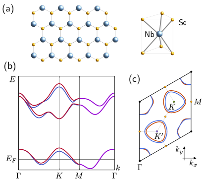
Figure 1: Lattice, band structure and Brillouin zone of NbSe₂. (a) Top view of the lattice and the trigonal prismatic unit cell. (b) The six spin-resolved bands of NbSe₂ closest to the Fermi energy $E_{F}$. They have been obtained within a tight-binding model involving three $d$ orbitals of the Nb atoms. The Ising spin-orbit coupling induces a large splitting of the valence bands at the $K$ and $K^{\prime}$ points. (c) The Brillouin zone of NbSe₂, with spin-resolved Fermi surface pockets near the $K,K^{\prime}$ and $\Gamma$ points.

II.1 A low energy minimal model for NbSe₂

Superconductivity is a low energy phenomenon originating from the binding of electrons residing close to the Fermi energy. Hence, in the following we will only consider the valence bands and will focus on the features close to the Fermi energy. Furthermore, as the mechanism we shall discuss strongly relies on the existence of disconnected Fermi surfaces related by time reversal symmetry, we shall focus on the dispersion around the $K$ and $K^{\prime}$ valleys and disregard the contribution of the $\Gamma$ Fermi surface. The latter can admit at most $s$-wave pairing Shaffer et al. (2020) and is not relevant for the mechanism discussed here, leading to a dominant $f$-wave channel.

Our aim is to develop a minimal low energy model for superconductivity in NbSe₂. Hence, instead of using the full tight-binding models mentioned above, we restrict the following discussion to a hyperbolic fit to the dispersion in the two valleys. The fitting parameters are obtained from two tight-binding parametrizations Kim and Son (2017); He et al. (2018), as discussed below. For simplicity, the trigonal warping far from the Dirac points is neglected. Then the hyperbolic dispersion for a particle of spin $\sigma$ and momentum $\mathbb{k}$ measured from the Dirac point $\tau K$, with $\tau=\pm$, is written as

$$\varepsilon_{\tau\sigma}(\mathbb{k})={\epsilon}_{\tau\sigma}^{0}+m_{\tau\sigma}-\sqrt{(\hbar v_{F,\tau\sigma})^{2}\mathbb{k}^{2}+m_{\tau\sigma}^{2}}\,.$$ (1)

In the above equation $v_{F,\tau\sigma}$ is the Fermi velocity, $m_{\tau\sigma}$ is a mass-like parameter and $\epsilon_{\tau\sigma}^{0}$ the upper limit of the band, i.e. the energy directly at the $\tau K$ point. Since time-reversal symmetry is preserved by the SOC, it holds $\varepsilon_{\tau\sigma}(\mathbb{k})=\varepsilon_{-\tau-\sigma}(-\mathbb{k}):=\varepsilon_{\bar{\tau}\bar{\sigma}}(\bar{\mathbb{k}})$, where we used the shorthand notation $-\mathbb{k}:=\bar{\mathbb{k}}$, $-\tau:=\bar{\tau}$ and $-\sigma:=\bar{\sigma}$. This symmetry allows us to restrict our considerations to the $K$ valley by introducing the pseudospin indices

$$i=\left\{\begin{matrix}1&\ \text{for}&(K,\uparrow)\\ 2&\ \text{for}&(K,\downarrow)\end{matrix}\right.\,,\quad\bar{i}=\left\{\begin{matrix}\bar{1}&\ \text{for}&(K^{\prime},\downarrow)\\ \bar{2}&\ \text{for}&(K^{\prime},\uparrow)\end{matrix}\right..$$ (2)

Here, $i=1\,(2)$ denotes the upper (lower) band in the $K$ valley, while $\bar{i}=\bar{1}\,(\bar{2})$ are the time-reversed upper (lower) bands in the $K^{\prime}$ valley. With this notation the energy relative to the chemical potential $\mu$ in the $K$ valley can be written as

$$\xi_{i}(\mathbb{k})=\varepsilon_{i}(\mathbb{k})-\mu={\xi}_{i}^{0}+m_{i}-\sqrt{(\hbar v_{F,i})^{2}\mathbb{k}^{2}+m_{i}^{2}}\,,$$ (3)

where $\xi_{i}^{0}=\epsilon_{i}^{0}-\mu$.

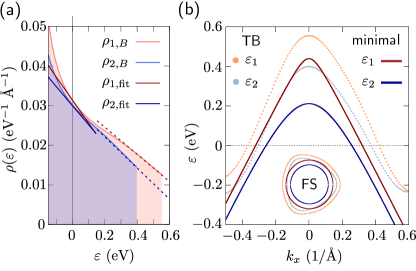
Figure 2: Density of states (DOS) and energy bands in the minimal model. (a) DOS in the $K$ valley associated to the spin-orbit split valence bands. The coloured regions depict the DOS $\rho_{1,2,\textnormal{TB}}$ obtained numerically from the tight-binding model. The solid lines are the linear fits $\rho_{1,2,\textnormal{fit}}$ to those DOS close to the Fermi level, used to estimate the parameters of the effective model. Dashed lines mark the linear fits to the DOS higher on the Dirac cone, for comparison. (b) The tight-binding and the effective model dispersion and (in the inset) the Fermi surfaces in the $K$ valley, with $k_{x}$ measured with respect to $K$. Solid lines show results for the effective model, the dotted curves display the numerical tight-binding bands with the parametrization in Kim and Son (2017).

II.2 Density of states

Making use of the approximate band structure Eq. (3), we can get to an expression for the band resolved density of states (DOS) per unit area at the $K$-Dirac cone. We find

$$\rho_{i}(\varepsilon):=\frac{1}{N\Omega}\sum_{\mathbb{k}}\delta(\varepsilon-\varepsilon_{i}(\mathbb{k}))=\left(\rho_{Fi}-d_{i}\varepsilon\right)\theta(\epsilon_{i}^{0}-\varepsilon)\,,$$ (4)

where $N$ is the number of Nb atoms in the lattice, with the factor of the linear term $d_{i}=1/(2\pi(\hbar v_{F,i})^{2})$ and the constant term $\rho_{Fi}=({\epsilon}_{i}^{0}+m_{i})d_{i}:=\tilde{\epsilon_{i}}d_{i}$. Hence, the DOS directly at the chemical potential is given by

$$\rho_{i}(\mu)=\left(\rho_{Fi}-d_{i}\mu\right)\,\theta(\epsilon_{i}^{0}-\mu)=({\xi}_{i}^{0}+m_{i})d_{i}\;\theta(\xi_{i}^{0})\,.$$ (5)

We have two guiding principles in constructing the minimal model:
(i) The DOS for each band must be the same as in the tight-binding model within the relevant energy range around the Fermi level.
(ii) The spin-orbit splitting between the two bands at the Fermi level should be correct (this will be important when we consider the evolution of the gap in magnetic field).
In the following we set the zero of the energy at the Fermi level of the normal system. We can fix the free parameters $\tilde{\epsilon}_{i}$ and $v_{F,i}$ of the minimal model by requiring that the DOS in Eq. (4) assumes the value $\rho_{Fi}$ at the Fermi level and its slope is determined by $d_{i}$. One of the masses is chosen arbitrarily to be $m_{1}=0.1$ eV. The value of $m_{2}$ (and hence also the parameter $\epsilon_{2}^{0}=\tilde{\epsilon}_{2}-m_{2}$) is set by fixing the values of the spin orbit splitting at the Fermi level. Explicitly, we require

$$\Delta_{\text{SOC}}:=\varepsilon_{1}(k_{F,1})-\varepsilon_{2}(k_{F,1})=-\varepsilon_{2}(k_{F,1})\,,$$ (6)

where $k_{F,i}$ are the Fermi momenta of the two bands obtained in full tight-binding, satisfying $\varepsilon_{i}(k_{F,i})=0$. The value of $\Delta_{\text{SOC}}$ is taken from the tight-binding calculation as an average between the spin-orbit splitting in the $\Gamma K$ and in the $KM$ direction. The results of the fitting procedure are illustrated in Fig. 2 where the tight-binding bands and DOS were calculated using the parameter set given in [He et al., 2018], denoted in the following as set $B$. An alternative setKim and Son (2017) (plots not shown) is denoted as set $A$. The resulting minimal model parameters are shown in Table 1.

set	$i$	$\rho_{Fi}$	$d_{i}$	$\epsilon_{i}^{0}$	$\tilde{\epsilon}_{i}$	$\hbar v_{F,i}$	$m_{i}$
$A$Kim and Son (2017)	1	0.0385	0.09	0.328	0.428	1.33	0.1
	2	0.046	0.13	0.199	0.354	1.106	0.155
$B$He et al. (2018)	1	0.0314	0.0583	0.439	0.539	1.652	0.1
	2	0.03	0.0481	0.209	0.624	1.819	0.415

Table 1: Parameters from the linear fit to the DOS and the SOC splitting at the Fermi energy. Units for $\rho_{Fi}$, $d_{i}$ and $\hbar v_{F,i}$ are ${\text{eV}}^{-1}{$\mathrm{\SIUnitSymbolAngstrom}$}^{-2}$, ${\text{eV}}^{-2}{$\mathrm{\SIUnitSymbolAngstrom}$}^{-2}$ and eVÅ, respectively. The values of spin-orbit splitting at the Fermi level are $\Delta_{\text{SOC}}^{A}=0.0253$ eV and $\Delta_{\text{SOC}}^{B}=0.092$ eV.

III Two-bands superconductivity and coupled gap equations

We now turn to the mechanism inducing the two-bands superconducting phase in NbSe₂. For this purpose we will focus on the two partially occupied bands around the Fermi level which give rise to the spin separated Fermi surfaces at the $K$ and $K^{\prime}$ points discussed in the previous section. Another smaller pocket might be found at the $\Gamma$ point; however it will not be part of the further discussion since it is expected to only play a subordinate role Shaffer et al. (2020). Instead of the conventional pairing mechanism that leads to the formation of Cooper pairs, i.e. the phonon-mediated attraction of two electrons, we will now consider the Coulomb repulsion of such electrons and hence an unconventional pairing. While phonons are believed to contribute the dominant mechanism for bulk NbSe₂ Valla et al. (2004); Noat et al. (2015); Heil et al. (2017); Sanna et al. (2022), this should not be the case for the monolayer caseWan et al. (2021). Further, Coulomb interactions are not well screened in a monolayer, and hence short range and long contributions should be included.

According to these considerations, we start from an interacting Hamiltonian with conventional, spin independent, Coulomb interaction. By retaining only scattering processes among time-reversal related Cooper pairs, the total Hamiltonian is the sum of a single particle and an interaction part,

$$\hat{H}_{\text{tot}}=\hat{H}_{\text{sp}}+\hat{H}_{\text{int}}\,.$$ (7)

The single particle contribution follows from the minimal model from the previous section and reads

$$\hat{H}_{\text{sp}}=\sum_{\sigma\tau\mathbb{k}}\varepsilon_{\tau\sigma}(\mathbb{k})\hat{c}^{\dagger}_{\mathbb{k}\tau\sigma}\hat{c}_{\mathbb{k}\tau\sigma}\,,$$ (8)

with the dispersion provided by Eq. (1). The interaction Hamiltonian Roldán et al. (2013)

$$\hat{H}_{\text{int}}=\frac{1}{2}\sum_{\sigma\tau\mathbb{k}\mathbb{k}^{\prime}}\big{[} V^{\text{intra}}_{\mathbb{k}\mathbb{k}^{\prime}}\hat{c}^{\dagger}_{\mathbb{k}\tau\sigma}\hat{c}^{\dagger}_{\bar{\mathbb{k}}\bar{\tau}\bar{\sigma}}\hat{c}_{\bar{\mathbb{k}}^{\prime}\bar{\tau}\bar{\sigma}}\hat{c}_{\mathbb{k}^{\prime}\tau\sigma}$$

$$+ V^{\text{inter}}_{\mathbb{k}\mathbb{k}^{\prime}}\hat{c}^{\dagger}_{\bar{\mathbb{k}}\bar{\tau}\sigma}\hat{c}^{\dagger}_{\mathbb{k}\tau\bar{\sigma}}\hat{c}_{\bar{\mathbb{k}}^{\prime}\bar{\tau}\bar{\sigma}}\hat{c}_{\mathbb{k}^{\prime}\tau\sigma}\big{]}$$ (9)

accounts for both intravalley and intervalley scattering processes. For an electron with momentum $\mathbb{k}$ and spin $\sigma$ that is located at the $K$ valley, its time-reversal partner will be located at $K^{\prime}$ with opposite momentum. Thus, as shown in Fig. 3, there are now two possible scattering mechanisms, mediated by $V^{\text{intra}}_{\mathbb{k}\mathbb{k}^{\prime}}$ and $V^{\text{inter}}_{\mathbb{k}\mathbb{k}^{\prime}}$, that can occur between the members of a pair. For an intravalley process the scattered electrons stay within their initial valley in $\mathbb{k}$-space, i.e. the valley index will be conserved. This means that the exchanged momentum $\mathbb{q=k-k^{\prime}}$ is small, which corresponds to a long-ranged interaction in real space. The intervalley scattering on the other hand describes a short ranged Coulomb interaction with a large exchanged momentum of the order of $2|\mathbb{K}|$. In this process the electrons swap their valley and hence $\tau$ flips its sign. Note that since the Coulomb interaction conserves spin, the intervalley scattering transforms a Cooper pair residing on the inner (outer) Fermi surface into a pair residing on the outer (inner) Fermi surface. This process thus couples the two condensates.

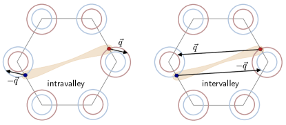
Figure 3: Superconductivity in monolayer TMDCs can arise from the interplay of repulsive long and short range interactions. On the left, a typical intravalley scattering process which involves small momentum transfer $\pm\vec{q}$ is shown. On the right, intervalley scattering with large momentum transfer $\pm\vec{q}$ is depicted. The scattered Cooper pairs are related by time reversal and hence reside in different valleys.

The two sums in Eq. (III) run over a shell around the Fermi surface whose thickness will be denoted as $\Lambda$. In fact, as in the conventional BCS theory, the restriction of the sums in momentum space to time-reversal partners is appropriate at low energies where only electrons in the vicinity of the Fermi energy are involved Bardeen et al. (1957). For a phonon-mediated interaction the shell thickness is in the order of the Debye energy $\hbar\omega_{\text{D}}$. Here we shall assume a shell thickness also in the meV range.

III.1 Mean field Hamiltonian

Due to the complexity of the scattering processes described by the interaction Hamiltonian Eq. (III), we simplify the problem by performing a mean field approximation Bardeen et al. (1957) on both interaction terms. By introducing the pairing functions

$$\Delta_{\tau\sigma}^{\text{intra}}(\mathbb{k}) =-\sum_{\mathbb{k}^{\prime}}V^{\text{intra}}_{\mathbb{k}\mathbb{k}^{\prime}}\langle\hat{c}_{\bar{\mathbb{k}}^{\prime}\bar{\tau}\bar{\sigma}}\hat{c}_{\mathbb{k}^{\prime}\tau\sigma}\rangle\,,$$

$$\Delta_{\tau\sigma}^{\text{inter}}(\mathbb{k}) =-\sum_{\mathbb{k}^{\prime}}V^{\text{inter}}_{\mathbb{k}\mathbb{k}^{\prime}}\langle\hat{c}_{\bar{\mathbb{k}}^{\prime}\bar{\tau}\sigma}\hat{c}_{\mathbb{k}^{\prime}\tau\bar{\sigma}}\rangle\,,$$ (10)

and by making use of the fermionic anticommutation relations, we can express the interaction Hamiltonian in the compact form

$$\hat{H}_{\text{int}}^{\text{mf}}=-\frac{1}{2}\sum_{\mathbb{k}\tau\sigma}\big{[}\Delta_{\tau\sigma}(\mathbb{k})\hat{c}^{\dagger}_{\mathbb{k}\tau\sigma}\hat{c}^{\dagger}_{\bar{\mathbb{k}}\bar{\tau}\bar{\sigma}}+(\Delta_{\tau\sigma}(\mathbb{k}))^{*}\hat{c}_{\bar{\mathbb{k}}\bar{\tau}\bar{\sigma}}\hat{c}_{\mathbb{k}\tau\sigma}\big{]}\,,$$

with the global gaps

$$\Delta_{\tau\sigma}(\mathbb{k})=\Delta_{\tau\sigma}^{\text{intra}}(\mathbb{k})-\Delta_{\tau\sigma}^{\text{inter}}(\mathbb{k})\,.$$ (11)

In Eq. (III.1) irrelevant constant terms, encapsulated in an overall contribution $C$, have been omitted. Notice that the hermiticity of the interaction Hamiltonian Eq. (III) together with the fermionic nature of the electronic operators ensure the property $\Delta_{\bar{\tau}\bar{\sigma}}(\bar{\mathbb{k}})=-\Delta_{\tau\sigma}(\mathbb{k})$, i.e., that the gap functions are odd under time reversal. This property allows us to write the total grandcanonical mean field Hamiltonian in terms of the pseudospin index $(i,\bar{i})$ introduced in the previous section

$$\hat{H}^{\text{mf}}-\mu\hat{N}-C= \sum\limits_{\mathbb{k},i=1,2}\xi_{i}(\mathbb{k})\left(\hat{c}^{\dagger}_{\mathbb{k}i}\hat{c}_{\mathbb{k}i}+\hat{c}^{\dagger}_{\bar{\mathbb{k}}\,\bar{i}}\hat{c}_{\bar{\mathbb{k}}\,\bar{i}}\right)$$

$$- \sum\limits_{\mathbb{k},i=1,2}\left(\Delta_{i}(\mathbb{k})\hat{c}^{\dagger}_{\mathbb{k}i}\hat{c}^{\dagger}_{\bar{\mathbb{k}}\,\bar{i}}+h.c.\right)\,,$$ (12)

where the dispersion relative to the chemical potential $\xi_{i}(\mathbb{k})$ was given in Eq. (3). It is noteworthy that for each of the two pseudospins, $(1,\bar{1})$ and $(2,\bar{2})$, the above expression has the BCS form, where the collective index $i$ plays the role of the conventional spin. Thus, the mean field Hamiltonian can be readily diagonalized by a conventional Bogoliubov transformation accounting for the full quasiparticle spectrum of the two-bands superconductor.

III.2 Bogoliubov transformation and coupled gap equations

For a quadratic Hamiltonian like in Eq. (III.1) the Bogoliubov transformation has the form

$$\begin{pmatrix}\hat{\gamma}_{\mathbb{k}i}\\ \hat{\gamma}_{\bar{\mathbb{k}}\,\bar{i}}^{\dagger}\end{pmatrix}=\begin{pmatrix}u_{\mathbb{k}i}&-v_{\mathbb{k}i}\\ v^{*}_{\mathbb{k}i}&u^{*}_{\mathbb{k}i}\end{pmatrix}\begin{pmatrix}\hat{c}_{\mathbb{k}i}\\ \hat{c}^{\dagger}_{\bar{\mathbb{k}}\,\bar{i}}\end{pmatrix},\ \ |u_{\mathbb{k}i}|^{2}+|v_{\mathbb{k}i}|^{2}=1\,,$$ (13)

where the condition on the sum of the coefficients $v_{\mathbb{k}i}$ and $u_{\mathbb{k}i}$ ensures the proper fermionic anticommutation relations of the quasi-particle operators $\hat{\gamma}_{\mathbb{k}i}$. By choosing for the coefficients the conventional BCS form

$$|u_{\mathbb{k}i}|^{2}=\frac{1}{2}\left(1+\frac{\xi_{i}(\mathbb{k})}{E_{i}(\mathbb{k})}\right),\quad|v_{\mathbb{k}i}|^{2}=\frac{1}{2}\left(1-\frac{\xi_{i}(\mathbb{k})}{E_{i}(\mathbb{k})}\right)\,,$$ (14)

with $E_{i}(\mathbb{k})=\sqrt{\big{(}\xi_{i}(\mathbb{k})\big{)}^{2}+\big{|}\Delta_{i}(\mathbb{k})\big{|}^{2}}$, we obtain the diagonalized mean-field Hamiltonian

$$\hat{H}^{\text{mf}}-\mu\hat{N}-C=\sum\limits_{\mathbb{k},i}E_{i}(\mathbb{k})\left(\hat{\gamma}_{\mathbb{k}i}^{\dagger}\hat{\gamma}_{\mathbb{k}i}+\hat{\gamma}_{\bar{\mathbb{k}}\,\bar{i}}^{\dagger}\hat{\gamma}_{\bar{\mathbb{k}}\,\bar{i}}\right)\,.$$ (15)

The simple and elegant expression above allows one to evaluate all the thermodynamic properties of the two-bands superconductor.

Of primary interest for us are the self-consistent equations for the gaps $\Delta_{1}$ and $\Delta_{2}$. In particular, we are asking if nontrivial solutions exist, and if they are compatible with a realistic parametrization for NbSe₂ or for other Ising superconducting TMDCs. Bogoliubov operators describe excitations in the superconductor in terms of an ensemble of non-interacting quasiparticles. The equilibrium occupation of the quasiparticle states is thus provided by the Fermi function according to $\langle\hat{\gamma}_{\mathbb{k}i}^{\dagger}\hat{\gamma}_{\mathbb{k}i}\rangle=f(E_{i}(\mathbb{k}))$, and $\langle\hat{\gamma}_{\mathbb{k}i}\hat{\gamma}^{\dagger}_{\mathbb{k}i}\rangle=1-f(E_{i}(\mathbb{k}))$. Starting from the definition of the gaps in Eq. (11) and expressing the averages in $\Delta_{\tau\sigma}^{\text{intra/inter}}(\mathbb{k})$ in terms of expectation values of Bogoliubov operators, yields for the two-component vector $\boldsymbol{\Delta}=(\Delta_{1}(\mathbb{k}),\Delta_{2}(\mathbb{k}))^{T}$ the coupled set of equations

$$\boldsymbol{\Delta}(\mathbb{k}) =-\sum_{\mathbb{k}^{\prime}}\cal{M}(\mathbb{k}^{\prime})\boldsymbol{\Delta}(\mathbb{k}^{\prime})\,,$$ (16)

$$\cal{M}(\mathbb{k}^{\prime})= \begin{pmatrix}V^{\text{intra}}_{\mathbb{k}\mathbb{k}^{\prime}}\chi_{1}(\mathbb{k}^{\prime})&&-V^{\text{inter}}_{\mathbb{k}\mathbb{k}^{\prime}}\chi_{2}(\mathbb{k}^{\prime})\\ -V^{\text{inter}}_{\mathbb{k}\mathbb{k}^{\prime}}\chi_{1}(\mathbb{k}^{\prime})&&V^{\text{intra}}_{\mathbb{k}\mathbb{k}^{\prime}}\chi_{2}(\mathbb{k}^{\prime})\end{pmatrix}\,.$$ (17)

The functions $\chi_{i}(\mathbb{k}^{\prime})$ incorporate the Fermi statistics of the quasiparticles and are given by

$$\chi_{i}(\mathbb{k})=\chi_{i}(\xi_{i}(\mathbb{k}))=\dfrac{1}{2E_{i}(\mathbb{k})}\tanh\left(\dfrac{\beta E_{i}(\mathbb{k})}{2}\right)\,,$$ (18)

with $\beta=1/k_{\text{B}}T$, $k_{\text{B}}$ Boltzmann constant and $T$ the temperature. Once the solution for the gaps within the $K$ valley is found, the gaps within the $K^{\prime}$ valley follow from $\Delta_{\bar{i}}(\mathbb{k})=-\Delta_{i}(-\mathbb{k})$. In the following we shall refer to $\Delta_{1}$ and $\Delta_{2}$ as the gaps of the outer and inner Fermi surfaces, respectively, of the $K$ valley.

III.3 Temperature dependence of the inner and outer gaps

Our first task will now be to find nontrivial solutions of the gap equation (16). For general $\mathbb{k}$-dependent interaction potentials this is a quite difficult task, as it is already the case for the conventional BCS gap equation. Here the off-diagonal terms, introduced by a non-vanishing intervalley potential $V^{\text{inter}}_{\mathbb{k}\mathbb{k}^{\prime}}$, give rise to a coupling between the $\Delta_{1}(\mathbb{k})$ and $\Delta_{2}(\mathbb{k})$ gaps which further complicates matters. For this reason we shall focus on constant interactions in the following discussion and remember that $V^{\text{intra}}_{\mathbb{k}\mathbb{k}^{\prime}},V^{\text{inter}}_{\mathbb{k}\mathbb{k}^{\prime}}$ describe long- and short-ranged parts, respectively, of the Coulomb repulsion in real-space. Qualitatively, these potentials can be conveniently described in terms of the screened interactions Roldán et al. (2013)

$$U^{\text{intra}}_{\mathbb{k}\mathbb{k}^{\prime}} :=V^{\text{intra}}_{\mathbb{k}\mathbb{k}^{\prime}}\,N\Omega\approx\dfrac{2\pi e^{2}}{\epsilon(|\mathbb{k}-\mathbb{k}^{\prime}|+q_{\text{TF}})}\,,$$ (19)

$$U^{\text{inter}}_{\mathbb{k}\mathbb{k}^{\prime}} :=V^{\text{inter}}_{\mathbb{k}\mathbb{k}^{\prime}}\,N\Omega=U_{\text{inter}}\,.$$ (20)

In Eq. (19) $\epsilon$ is the dielectric constant of the environment, and $q_{\text{TF}}=2\pi e^{2}\rho(\mu)/\epsilon$ the Thomas-Fermi momentum which describes the screening of the long-range tail of the Coulomb interaction. In this case $\rho(\mu)=\rho_{1}(\mu)+\rho_{2}(\mu)$ is the total DOS at the Fermi level, given by the sum of both DOS in Eq. (5), since we neglected contributions coming from the $\Gamma$ pockets. In the second equality, Eq. (20), the quantity $U_{\text{inter}}$ is of the order of the product $(e^{2}/2a)\Omega$, with $a$ the interatomic distance and $\Omega$ the size of the unit cell. It describes the leading term in the short-ranged Coulomb interaction of two electrons with opposite spin which occupy the same Nb $4d$ orbital. Although the exact value of $U_{\text{inter}}$ is not known, it lies in the few eV range Guinea and Uchoa (2012).
The expression $U^{\text{intra}}_{\mathbb{k}\mathbb{k}^{\prime}}$ can further be simplified by assuming that $q_{\text{TF}}$ is much larger than all of the considered exchanged momenta $|\mathbb{k}-\mathbb{k}^{\prime}|\sim\mathbb{k}_{F,i}$ which are of the order of the Fermi momentum for one of the two bands. Note that this assumption can only be justified for not too large $\epsilon$ which would otherwise yield a rather small value for $q_{\text{TF}}$. Here we shall simply assume that this is indeed fulfilled. Hence, the intravalley potential also assumes a constant form,

$$U^{\text{intra}}_{\mathbb{k}\mathbb{k}^{\prime}}\approx\frac{2\pi e^{2}}{\epsilon q_{TF}}=\frac{1}{\rho(\mu)}\equiv U_{\text{intra}}\,.$$ (21)

Due to the now constant interactions and the fact that the right hand side of the gap equation in Eq. (16) only depends on $\mathbb{k}$ via the two potentials, the gap vector will be isotropic within each valley, i.e. $\mathbb{\Delta}(\mathbb{k})=\mathbb{\Delta}$. Defining $\alpha_{i}:=\frac{1}{N\Omega}\sum_{\mathbb{k}}\chi_{i}(\mathbb{k})$, the gap equation can now be written in the compact form

$$\mathbf{M}\mathbb{\Delta}=\left[\mathbf{1}+\begin{pmatrix}\ \,U_{\text{intra}}\alpha_{1}&&-U_{\text{inter}}\alpha_{2}\\ -U_{\text{inter}}\alpha_{1}&&\ \,U_{\text{intra}}\alpha_{2}\end{pmatrix}\right]\mathbb{\Delta}=0\,.$$ (22)

Non-trivial solutions of the gap equation require a vanishing determinant of the matrix $\mathbf{M}$. By introducing the potential $U_{\text{attr}}=(U_{\text{intra}}^{2}-U_{\text{inter}}^{2})/U_{\text{intra}}$, we obtain

$$\det\mathbf{M} =U_{\text{attr}}U_{\text{intra}}\alpha_{1}\alpha_{2}+U_{\text{intra}}(\alpha_{1}+\alpha_{2})+1=0\,.$$ (23)

Since both $\alpha_{i}$’s and the potentials $U_{\text{intra}},U_{\text{inter}}$ are positive, the above condition can only be fulfilled if $U_{\text{attr}}<0$, i.e. $U_{\text{intra}}<U_{\text{inter}}$, leading to an attractive potential. Note that since the intervalley scattering enters quadratically in the definition of $U_{\text{attr}}$, its sign is not relevant here. Also, in the absence of intervalley scattering, $U_{\text{inter}}=0$, only the trivial solution $\boldsymbol{\Delta}=0$ exists for repulsive intravalley interaction. The phase diagram for various combinations of the signs and relative strengths of the interactions is discussed in Sec. III.4.

The sum over momenta in the definition of the quantities $\alpha_{i}$ can be evaluated by transforming it into an energy integral

$$\alpha_{i} =\dfrac{1}{N\Omega}\sum\limits_{\mathbb{k}}\chi_{i}(\mathbb{k})=\int_{-\Lambda}^{\Lambda}\mathrm{d}\xi\,\left(\rho_{i}(\mu)-d_{i}\xi\right)\chi_{i}(\xi)\theta(\xi_{i}^{0}-\Lambda)$$

$$=\rho_{i}(\mu)\int_{-\Lambda}^{\Lambda}\mathrm{d}\xi\,\chi_{i}(\xi)\theta(\xi_{i}^{0}-\Lambda)\,,$$ (24)

where the Heaviside function ensures that the integration interval is below the top of the valence bands. Since we assume that $\Lambda$ defines a small energy interval around the Fermi energy, this requirement is automatically satisfied. Usually in the computation of the integral one would approximate the DOS $\rho_{i}(\varepsilon)$ with its value $\rho_{i}(\mu)$ at the Fermi level. Here, we naturally only get contributions from the latter since the linear term in the DOS leads to an odd integrand which vanishes upon integration.

Let us now for a moment consider NbSe₂ with a strongly shifted Fermi level, close to the top of the valence bands. According to the definition Eq. (5), the DOS at the Fermi level $\rho_{i}(\mu)$ vanishes if $\xi_{i}^{0}<0$. We can thus differentiate between two configurations which could possibly lead to finite $\alpha_{i}$. In the first one, the chemical potential $\mu$ lies between the top of the upper and the lower band ($\xi_{1}^{0}>0,\ \xi_{2}^{0}<0$); in the second one $\mu$ is below the top of both bands ($\xi_{i}^{0}>0$). In the first scenario $\alpha_{2}=0$ and Eq. (23) leads to the familiar BCS gap equation, however now with the repulsive interaction $U_{\text{intra}}>0$. As it is well-known, the BCS gap equation allows non-trivial solutions only for attractive potentials. Hence in this case the condition for finite gaps in Eq. (23) is not fulfilled and Eq. (22) is only solved by $\Delta_{i}=0$. This means that a superconducting phase cannot exist for such range of chemical potentials. Only the second scenario, where both interactions can take place, is relevant for the further discussion. Notice that this interdependence of the two gaps implies that the there exists a single critical temperature $T_{c}$ at which both gaps vanish. Its expression is derived in analytical form below.

III.3.1 The critical temperature

At the critical temperature both gaps will have vanished and the superconducting state collapses. Hence, we simply set $\Delta_{i}=0$ in $\alpha_{i}(T_{c})$. With the assumption that the energy cutoff is much larger than the critical temperature, i.e. $\Lambda\gg k_{B}T_{c}$, the integrals can be solved analytically

$$\alpha_{i}(T_{c})=\rho_{i}(\mu)\int_{0}^{2\Lambda/k_{B}T_{c}}\mathrm{d}x\,\dfrac{\tanh x}{x}\approx-\rho_{i}(\mu)\ln{\dfrac{T_{c}}{\theta}},$$ (25)

with the characteristic temperature $\theta=2e^{\gamma}\Lambda/\pi k_{B}$ and the Euler-Mascheroni constant $\gamma\approx 0.577$. Inserting these expressions into Eq. (23), we find a polynomial of degree two in $\ln{\frac{T_{c}}{\theta}}$ whose solutions can be used to obtain the critical temperaturenot (a)

$$\dfrac{T_{c}}{\theta}=\exp\left[\dfrac{1}{2U_{\text{attr}}}\dfrac{1}{r}\left(1+\sqrt{1-2\dfrac{U_{\text{attr}}}{U_{\text{intra}}}\dfrac{r}{\bar{\rho}}}\ \right)\right]\,.$$ (26)

Note that the DOS of the two bands $\rho_{1}(\mu)$ and $\rho_{2}(\mu)$ only enter in the symmetrical combinations

$$\dfrac{1}{r}=\frac{1}{\rho_{1}}+\frac{1}{\rho_{2}}\,,\quad\bar{\rho}=\dfrac{\rho_{1}+\rho_{2}}{2}\,.$$ (27)

When for similar DOS we approximate the value of $1/r$ by $2/\bar{\rho}$, the simplified expression for $T_{c}$ reads

$$T_{c}\simeq\theta\;\exp\left(-\frac{1}{\bar{\rho}(U_{\text{inter}}-U_{\text{intra}})}\right).$$ (28)

For repulsive interactions this result stresses again the importance of the local repulsion winning over the long-range one, encoded in our $U_{\text{inter}}>U_{\text{intra}}$ requirement. As we shall discuss in Sec. III.3.3, depending on the signs and relative strengths of the potentials we may have to choose the other root of Eq. (23).
As the temperature is lowered below $T_{c}$, the gaps start to grow and reach their maximal value at zero temperature. Some properties of the zero temperature gaps are elucidated below.

III.3.2 Zero temperature gaps

The gaps at absolute zero cannot be given in an explicit closed form. One can, however, derive an equation whose solution yields them. Here, instead of writing $\Delta_{i}(T=0)$, we simply keep the notation $\Delta_{i}$ and remember that these are actually the gaps at $T=0$. Then, as the temperature approaches zero, the hyperbolic tangent reaches one and the integral yielding $\alpha_{i}(T=0)$ can again be computed analytically. Further assuming $\Lambda\gg|\Delta_{i}|$, one finds the asymptotic form

$$\alpha_{i}=\rho_{i}\int_{0}^{\Lambda/|\Delta_{i}|}\mathrm{d}x\dfrac{1}{\sqrt{1+x^{2}}}\approx-\rho_{i}\ln\dfrac{|\Delta_{i}|}{2\Lambda}:=-\rho_{i}x_{i}\,,$$ (29)

with the dimensionless quantity $x_{i}=\ln\frac{|\Delta_{i}|}{2\Lambda}$. By making use of the condition in Eq. (23) one can first get to a relation between $|\Delta_{1}|$ and $|\Delta_{2}|$. Afterwards, using the first or the second row of the gap equation (22), leads to

$$U_{\text{inter}}\exp\left[\dfrac{1}{\rho_{j}U_{\text{intra}}}\dfrac{1-\rho_{i}U_{\text{intra}}x_{i}}{1-\rho_{i}U_{\text{attr}}x_{i}}\right]$$

$$+U_{\text{intra}}(1-\rho_{i}U_{\text{attr}}x_{i})e^{x_{i}}=0\,.$$ (30)

In the above equation the index $j$ always refers to the opposite of $i$, i.e. if $i=1\ (2)$ then $j=2\ (1)$. When solving numerically the above expression in terms of $x_{i}$ we can thus get to the absolute values of both gaps $\Delta_{i}$.

By considering only the leading terms in the gap equation (22) we can find closed analytical expressions for the average gap $\bar{\Delta}:=(\Delta_{1}+\Delta_{2})/2$ and the gap difference $\delta\Delta:=(\Delta_{1}-\Delta_{2})/2$. Using the the DOS difference $\delta\rho:=(\rho_{1}-\rho_{2})/2$ and the already introduced average DOS $\bar{\rho}=(\rho_{1}+\rho_{2})/2$, we can now add and subtract the two rows of Eq. (22), arriving at

$$\bar{\Delta}\simeq(U_{\text{intra}}-U_{\text{inter}})\;(\bar{\rho}\bar{\Delta}+\delta\rho\,\delta\Delta)\,\ln\left|\frac{\bar{\Delta}}{2\Lambda}\right|,$$

$$\delta\Delta\simeq(U_{\text{intra}}+U_{\text{inter}})\;(\bar{\rho}\delta\Delta+\delta\rho\,\bar{\Delta})\,\ln\left|\frac{\bar{\Delta}}{2\Lambda}\right|,$$

where we have approximated $\ln(\Delta_{i}/(2\Lambda))\approx\ln(\bar{\Delta}/(2\Lambda))$. Keeping only the leading $\bar{\rho}\bar{\Delta}$ term in the first equation, we find

$$\left|\bar{\Delta}\right|\simeq 2\Lambda\;\exp\left(-\dfrac{1}{\bar{\rho}\,(U_{\text{inter}}-U_{\text{intra}})}\right).$$ (31)

The expression for the average gap $\bar{\Delta}$ is highly reminiscent of the standard BCS result, linking in the same way the zero temperature gap and the critical temperature in Eq. (28).
From the second equation, when using the result of (31), we obtain

$$\delta\Delta\simeq-\,\bar{\Delta}\,\frac{\delta\rho}{\bar{\rho}}\;\frac{U_{\text{inter}}+U_{\text{intra}}}{2\,U_{\text{intra}}}.$$ (32)

The difference between the two gaps is proportional to the difference between their normal DOS, which is reasonable. A less intuitive property of $\delta\Delta$ is that its sign is opposite to that of $\delta\rho$ – in consequence, the band with larger $\rho_{i}(\mu)$ develops a smaller gap. Mathematically this is caused by the negative value of $\ln|\bar{\Delta}/(2\Lambda)|$. Physically, lower DOS in band $i$ means that the intravalley scattering, where both initial and final states are few, has lower amplitude than the intervalley scattering, where the final states belong to the band $j$, with higher DOS. The contrary is true for the band $j$.
Note that both (31) and (32) were derived assuming that $\bar{\Delta}>\delta\Delta$. For an $s$-wave pairing the two gaps have opposite signs (as will be discussed in Sec. III.3.3) and we would have to repeat our calculation for $\delta\Delta>\bar{\Delta}$ instead.

III.3.3 Numerical results and comparison with experiments

Getting to the full temperature dependence of the gaps requires numerical methods. Here, we used a self-consistent algorithm to solve the gap equation (16) together with the determinant condition in Eq. (23). The cutoff $\Lambda$ and the intervalley potential $U_{\text{inter}}$ are free parameters. They are fixed by requiring the critical temperature to be $T_{c}\simeq 2.83$ K and the average gap at zero temperature $\bar{\Delta}\simeq 0.4$ meV, in line with experimental estimates. While the critical temperature is $T_{c}\approx 7.2$K for bulk NbSe₂, it decreases with the number of layers Dvir et al. (2018). For example, Xi et al. Xi et al. (2016a) give the critical temperature for both the bulk and the monolayer system which are $T_{c}^{\text{bulk}}\approx 7.0\,$K and $T_{c}^{\text{mono}}\approx 3.0\,$K for exfoliated NbSe₂ monolayers. For molecular beam epitaxy grown monolayers the critical temperature has been found to vary between $T_{c}=0.9-2.4$ K Ugeda et al. (2016); Y. Xing et al. (2017); K. Zhao et al. (2019); Wan et al. (2021). A temperature dependence of the tunneling density of states, from which the average zero temperature gap was estimated to be around 0.4 meV is provided in Ref. [Wan et al., 2021]. We notice that, having fixed $\Lambda$ and $U_{\text{inter}}$, our predictions for the in-plane critical magnetic field discussed in the next section are parameter free. In Fig. 4 we provide numerical results for the evolution of the two gaps with temperature according to the TB parametrizations by Kim et al. Kim and Son (2017) and He et al. He et al. (2018), denoted by $A$ and $B$, respectively, in Table 1. For both models we set $\Lambda=10$ meV. Further parameters and the values of $\Delta_{i}(T=0)$ are listed in Table 2.

set	$U_{\text{intra}}$	$U_{\text{inter}}$	$\Delta_{1}(0)$	$\Delta_{2}(0)$	$\bar{\Delta}^{(30)}$	$\delta\Delta^{(31)}$
$A$	11.83	18.04	0.469	0.388	0.442	0.0495
$B$	16.29	24.77	0.42	0.44	0.43	-0.0123

Table 2: Interaction parameters and resulting zero temperature gaps. The difference in the interaction strengths arises due to the different values of the DOS at the Fermi level for the $A$ and $B$ sets. The units for the potentials are eVŲ, the units for the gaps are meV. The last two columns show the value of $\bar{\Delta}$ evaluated with Eq. (31) and $\delta\Delta$ evaluated with Eq. 32.

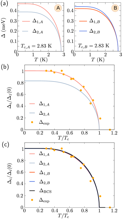
Figure 4: Temperature dependence of the outer and inner gaps, $\Delta_{1}$ and $\Delta_{2}$, respectively and universal scaling. (a) Numerical results showing the gaps’ evolution towards a common critical temperature. The two distinct parametrizations $A$ and $B$ in tables 1 and 2 were used. (b) Rescaled theoretical results for the parametrization $A$ and comparison with experimental points. The latter are digitized data from Fig. 3 in Ref. [Wan et al., 2021]. (c) A universal scaling of the gaps, independent of the chosen parametrization, is observed when dividing the theoretical gaps by their zero temperature value, and the temperature by the critical temperature.

As shown in Fig. 4(a), we find two finite gaps with the same critical temperature and which assume their largest values at zero temperature. The size of the gaps slightly depends on the chosen parametrization but the qualitative behavior is rather similar. Fig. 4(b) shows a comparison of the experimental dataWan et al. (2021), and the theoretical predictions with the $A$ parametrization. Notice that the evolution of the data points is compatible with the existence of the two gaps. Finally, Fig. 4(c) demonstrates that our predictions become BCS-like and independent of the specific parametrization when the temperature is rescaled by the critical temperature and the gaps by their respective zero temperature values.
Our approximate formulae (31) and (32) work well in both models. In the model $A$ the average gap $\bar{\Delta}$ differs by about 3% from the numerical result, while in the model $B$ (where the two bands are more similar) the two results agree up to 1%. The gap differences $\delta\Delta$ in both models are overestimated by about 20%.

It is by now well established that bulk NbSe₂ has two gaps, the second gap being due to the electrons in the Se pocket around the $\Gamma$ point Noat et al. (2015). Recent tunnel junction spectroscopic measurements of NbSe₂ devices with few layers have shown that the second gap grows weaker with decreasing number of layers,Dvir et al. (2018) becoming invisible in a bilayer deviceKuzmanović et al. (2021). Likewise, the scanning tunneling microscope (STM) measurements of monolayer devices in Ref. [Wan et al., 2021] do not display clear signatures of a second gap.
In order to establish whether the second gap would be at all visible in the $\text{d}I/\text{d}V$ characteristics of an STM, we calculated the tunneling density of statesTinkham (2004) for both parametrizations, $A$ and $B$, of our effective model. The results are shown in Fig. 5.

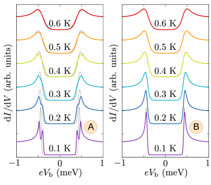
Figure 5: Differential conductance vs bias voltage of monolayer NbSe₂ at several temperatures. This quantity is proportional to the tunneling density of states. In both tight-binding parametrizations $T_{c}=2.83$ K. Thin grey lines correspond to the tunneling DOS with only one gap $\bar{\Delta}$. The two gaps are still recognizable at $T\approx 0.1\,T_{c}$ for the $A$, but not for the $B$ set. At higher temperatures, the gaps merge and are not visible in the differential conductance, which is also almost indistinguishable from the case of one gap $\bar{\Delta}$.

The two gaps are clearly visible in the $A$ model at $T=0.1$ K. Nevertheless, as the temperature rises, their quasiparticle peaks merge and at $T=0.4$ K only a shallower slope indicates that two gaps are present. With the $B$ parametrization the two gaps are too similar in magnitude to be clearly distinguishable even at $T=0.1$ K. Thus in order to distinguish the two gaps the tunneling experiments would have to be carried out at very low temperatures.

III.4 Symmetries of the inner and outer gaps

The symmetry of the gap is defined by its behavior under the reflection of its momentum, i.e. for $s,d$-wave symmetry $\Delta_{\tau\sigma}(\mathbb{k})=\Delta_{\bar{\tau}\sigma}(-\mathbb{k})$ while for $p,f$-wave $\Delta_{\tau\sigma}(\mathbb{k})=-\Delta_{\bar{\tau}\sigma}(-\mathbb{k})$. In systems with hexagonal lattice and small Fermi surfaces two types of symmetry allow an isotropic gap, the $s$ and $f$ symmetryBlack-Schaffer and Honerkamp (2014), as illustrated in Fig. 6(a). To see which one applies to our case, we recall that the fermionic anticommutation rules relate the gaps of opposite momenta and spins according to $\Delta_{\tau\sigma}(\mathbb{k})=-\Delta_{\bar{\tau}\bar{\sigma}}(-{\mathbb{k}})$. From the local isotropy of the gaps, it also follows that

$$\Delta_{\tau\sigma}(\mathbb{k})=\Delta_{\tau\sigma}(-{\mathbb{k}})\,.$$ (33)

Let us start by considering the easier case of zero SOC. In this case $\chi_{1}(\mathbb{k})=\chi_{2}(\mathbb{k})$ (which already implies $|\Delta_{1}|=|\Delta_{2}|$), and hence $\alpha:=\alpha_{1}=\alpha_{2}$ in Eq. (22) can be factorized from the matrix,

$$\left(\begin{array}[]{c}\Delta_{1}\\[5.69054pt] \Delta_{2}\end{array}\right)=-\alpha\left(\begin{array}[]{cc}U_{\text{intra}}&-U_{\text{inter}}\\[5.69054pt] -U_{\text{inter}}&U_{\text{intra}}\end{array}\right)\left(\begin{array}[]{c}\Delta_{1}\\[5.69054pt] \Delta_{2}\end{array}\right).$$ (34)

The first row of this matrix equation yields

$$\Delta_{1}=\frac{1+\alpha U_{\text{intra}}}{\alpha U_{\text{inter}}}\Delta_{2},$$ (35)

while the requirement of the existence of non-trivial solutions, Eq. (23), implies

$$\alpha_{\pm}=-\frac{1}{U_{\text{intra}}\mp U_{\text{inter}}}.$$ (36)

Hence, $\Delta_{1}=\pm\Delta_{2}$; i.e. in the absence of SOC the two gaps have the same amplitude but not necessarily the same sign. Since $\alpha$ is a sum of non-negative numbers, it must be positive. Depending on the sign and relative strength of $U^{\text{intra}}$ and $U^{\text{inter}}$ either one, none, or both of $\alpha_{\pm}$ are positive. Hence, according to the properties of the $s$ and $f$ gaps upon reflection of $\mathbb{k}$, we conclude

$$\begin{array}[]{l l l}\alpha_{+}>0&\quad\rightarrow\quad\Delta_{1}\,\Delta_{2}>0,&\quad\textnormal{$f$-wave},\\[5.69054pt] \alpha_{-}>0&\quad\rightarrow\quad\Delta_{1}\,\Delta_{2}<0,&\quad\textnormal{$s$-wave}.\end{array}$$ (37)

When both $\alpha_{\pm}>0$, the dominant is that one which results in greater energy gain upon condensation, i.e. in the larger amplitude of the gap. From Eq. (29) we see that the smaller $\alpha$ results in the larger gap. Therefore $\alpha_{+}\lessgtr\alpha_{-}$ results in a dominant gap with $f$ ($s$) symmetry.

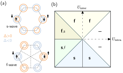
Figure 6: Symmetries of the superconducting gaps induced by spin conserving interactions in the absence of spin-orbit coupling (the two Fermi surfaces in each pocket are drawn as split only for clarity). (a) In a hexagonal lattice with Fermi surfaces around the Dirac valleys the two symmetries consistent with locally isotropic gaps are of the $s$ or $f$ type. (b) Leading gap symmetries when two competing scattering processes can take place, depending on the sign and relative strength of $U^{\text{intra}}$ and $U^{\text{inter}}$, and without SOC. When only one, repulsive, interaction is present, pairing does not occur.

When we include the effects of SOC, the two gaps become mixtures of the $s$ and $f$ character. In particular, because $\Delta_{i}(\mathbb{k})=-\Delta_{\bar{i}}(\bar{\mathbb{k}})$, then it holds for the average and difference gaps

$$\begin{array}[]{l l}{\Delta}_{K}=\frac{1}{2}(\Delta_{1}+\Delta_{2}):&\quad{\Delta}_{K}(\mathbb{k})=-{\Delta}_{\bar{K}}(\bar{\mathbb{k}})\quad(f)\,,\\[5.69054pt] \delta\Delta_{K}=\frac{1}{2}(\Delta_{1}-\Delta_{2}):&\quad\delta\Delta_{K}(\mathbb{k})=\delta\Delta_{\bar{\text{K}}}(\bar{\mathbb{k}})\quad(s)\,.\end{array}$$ (38)

Whether $\Delta_{K}$ or $\delta\Delta_{K}$ determines the prevalent symmetry depends on the sign of $\Delta_{1}\Delta_{2}$. In the limit of vanishing SOC we see again that with $\Delta_{1}\Delta_{2}>0$ the dominant gap is $\Delta_{K}$ i.e. $f$-wave, while for $\Delta_{1}\Delta_{2}<0$ the main gap is $\delta\Delta_{K}$ with $s$-wave symmetry.

IV Effects of an in-plane field

We now turn to the effect of an in-plane field on the superconducting state of monolayer NbSe₂. We are mostly interested in the temperature dependence of the critical magnetic field $B_{c}(T)$. We start by first considering the system without electronic interactions but with an additional magnetic field $\mathbb{B}=B\hat{e}_{x}$ along the $x$-axis. The single particle grandcanonical Hamiltonian at finite magnetic fields is

$$\hat{H}_{\text{B}}-\mu\hat{N}=\sum\limits_{\mathbb{k}\tau\sigma}\xi_{\tau\sigma}(\mathbb{k})\hat{c}_{\mathbb{k}\tau\sigma}^{\dagger}\hat{c}_{\mathbb{k}\tau\sigma}+\mu_{\text{B}}B\sum\limits_{\mathbb{k}\tau\sigma}\hat{c}_{\mathbb{k}\tau\sigma}^{\dagger}\hat{c}_{\mathbb{k}\tau\bar{\sigma}}\,,$$ (39)

where $\mu_{\text{B}}$ is the Bohr magneton. The above Hamiltonian can be diagonalized using the Ansatz

$$\begin{pmatrix}\hat{c}_{\mathbb{k}\tau\uparrow}\\ \hat{c}_{\mathbb{k}\tau\downarrow}\end{pmatrix}=\begin{pmatrix}a_{\mathbb{k}\tau}&b_{\mathbb{k}\tau}\\ -b_{\mathbb{k}\tau}&a_{\mathbb{k}\tau}\end{pmatrix}\begin{pmatrix}\hat{f}_{\mathbb{k}\tau+}\\ \hat{f}_{\mathbb{k}\tau-}\end{pmatrix},\ \ |a_{\mathbb{k}\tau}|^{2}+|b_{\mathbb{k}\tau}|^{2}=1\,.$$ (40)

A possible choice of the field-dependent parameters is

$$\left.\begin{matrix}a_{\mathbb{k}\tau}\\ b_{\mathbb{k}\tau}\end{matrix}\right\}=\pm\sqrt{\dfrac{1}{2}\left(1\pm\dfrac{\delta\xi_{\tau}(\mathbb{k})}{\sqrt{(\delta\xi_{\tau}(\mathbb{k}))^{2}+(\mu_{B}B)^{2}}}\right)}\,,$$ (41)

with $2\delta\xi_{\tau}(\mathbb{k})=\xi_{\tau\uparrow}(\mathbb{k})-\xi_{\tau\downarrow}(\mathbb{k})$. It results in the eigenenergies

$$\tilde{\xi}_{\tau n}(\mathbb{k}) =\bar{\xi}_{\tau}(\mathbb{k})\pm\sqrt{(\delta\xi_{\tau}(\mathbb{k}))^{2}+(\mu_{B}B)^{2}}\,,$$ (42)

where $2\bar{\xi}_{\tau}(\mathbb{k})=\xi_{\tau\uparrow}(\mathbb{k})+\xi_{\tau\downarrow}(\mathbb{k})$. These energies depend on the index $n=+,-$ and not on the spin $\sigma$ anymore since the magnetic field is oriented perpendicularly to the spin quantization axis set by the Ising SOC. Remembering the time-reversal relation $\xi_{\bar{\tau}\bar{\sigma}}(\bar{\mathbb{k}})=\xi_{\tau\sigma}(\mathbb{k})$ for the single-particle energies at zero magnetic field, one finds for the coefficients and energies the relations

$$a_{\mathbb{k}\tau}=-b_{\bar{\mathbb{k}}\bar{\tau}}\,,\quad\tilde{\xi}_{\tau n}(\mathbb{k})=\tilde{\xi}_{\bar{\tau}n}(\bar{\mathbb{k}})\,.$$ (43)

In order to describe the influence of the magnetic field on the superconducting phase one now has to express the mean-field interaction term in Eq. (III.1) in the new eigenbasis, i.e. in terms of the operators $\hat{f}_{\mathbb{k}\tau n}$. Doing so, one eventually arrives at the full mean-field Hamiltonian $\hat{H}=\hat{H}_{B}+\hat{H}_{\text{int}}^{\text{mf}}$ describing superconductivity in an Ising spin-orbit coupled TMDC monolayer in the presence of an in-plane magnetic field,

$$\hat{H}-\mu\hat{N}-C=\sum\limits_{\mathbb{k},n}\tilde{\xi}_{Kn}(\mathbb{k})\left(\hat{f}^{\dagger}_{\mathbb{k}Kn}\hat{f}_{\mathbb{k}Kn}+\hat{f}^{\dagger}_{\bar{\mathbb{k}}\bar{K}n}\hat{f}_{\bar{\mathbb{k}}\bar{K}n}\right)$$

$$+\sum\limits_{\mathbb{k},n}\Delta_{Kn}(\mathbb{k})\hat{f}^{\dagger}_{\mathbb{k}Kn}\hat{f}^{\dagger}_{\bar{\mathbb{k}}\bar{K}n}+h.c.$$ (44)

$$+\sum\limits_{\mathbb{k}}\Delta_{K\pm}(\mathbb{k})\left(\hat{f}^{\dagger}_{\mathbb{k}K+}\hat{f}^{\dagger}_{\bar{\mathbb{k}}\bar{K}-}-\hat{f}^{\dagger}_{\mathbb{k}K-}\hat{f}^{\dagger}_{\bar{\mathbb{k}}\bar{K}+}\right)+h.c.\,.$$

Here, we have defined the three new effective gaps which can be expressed in terms of the gaps $\Delta_{\tau\sigma}(\mathbb{k})$ (they obey $\Delta_{K\uparrow}=-\Delta_{K^{\prime}\downarrow}=\Delta_{1}$, $\Delta_{K\downarrow}=-\Delta_{K^{\prime}\uparrow}=\Delta_{2}$). The three new gaps are

$$\Delta_{K+}(\mathbb{k}) =-(a_{\mathbb{k}K}^{2}\Delta_{K\uparrow}(\mathbb{k})+b_{\mathbb{k}K}^{2}\Delta_{K\downarrow}(\mathbb{k}))\,,$$ (45)

$$\Delta_{K-}(\mathbb{k}) =b_{\mathbb{k}K}^{2}\Delta_{K\uparrow}(\mathbb{k})+a_{\mathbb{k}K}^{2}\Delta_{K\downarrow}(\mathbb{k})\,,$$ (46)

$$\Delta_{K\pm}(\mathbb{k}) =a_{\mathbb{k}K}b_{\mathbb{k}K}(\Delta_{K\uparrow}(\mathbb{k})-\Delta_{K\downarrow}(\mathbb{k}))\,.$$ (47)

The first two gap functions $\Delta_{Kn}(\mathbb{k})$ couple electrons of different $K$ valleys but the same energy, while $\Delta_{K\pm}(\mathbb{k})$ describes a pairing of electrons with different energies. In the latter case, it depends on the amplitude of the magnetic field values and of the superconducting pairing energies to which extent this term can contribute. Notice that Eq. (43) ensures that the new gaps $\Delta_{Kn}(\mathbb{k})$ have $f$-wave character while $\Delta_{K\pm}(\mathbb{k})$ is $s$-wave like, cf. also Eq. (38).

IV.1 Diagonalization of the mean field Hamiltonian in planar magnetic field

To get to the gap equation which now includes the magnetic field we need to evaluate the averages in the definition of the order parameter in Eq. (11). This requires to find the new set of Bogoliubov quasiparticles which diagonalize the Hamiltonian in Eq. (44). To this aim we first rewrite it in the Bogoliubov-de Gennes (BdG) form

$$\hat{H}-\mu\hat{N}-\tilde{C}=\sum\limits_{\mathbb{k}}\hat{\Psi}_{\mathbb{k}}^{\dagger}\hat{\mathcal{H}}_{\text{BdG}}(\mathbb{k})\hat{\Psi}_{\mathbb{k}}\,,$$ (48)

where we introduced the BdG Hamiltonian $\hat{\mathcal{H}}_{\text{BdG}}(\mathbb{k})$ and the Nambu spinor $\hat{\Psi}_{\mathbb{k}}$, respectively. They are given by

$$\hat{\mathcal{H}}_{\text{BdG}}(\mathbb{k}) =\begin{pmatrix}\tilde{\xi}_{K+}(\mathbb{k})&0&\Delta_{+}(\mathbb{k})&\Delta_{\pm}(\mathbb{k})\\ 0&\tilde{\xi}_{K-}(\mathbb{k})&-\Delta_{\pm}(\mathbb{k})&\Delta_{-}(\mathbb{k})\\ \Delta_{+}^{*}(\mathbb{k})&-\Delta^{*}_{\pm}(\mathbb{k})&-\tilde{\xi}_{K+}(\mathbb{k})&0\\ \Delta^{*}_{\pm}(\mathbb{k})&\Delta^{*}_{-}(\mathbb{k})&0&-\tilde{\xi}_{K-}(\mathbb{k})\end{pmatrix}\,,$$ (49)

where we used the abbreviation $\Delta_{Kn}=\Delta_{n}$, $\Delta_{K\pm}=\Delta_{\pm}$, and

$$\hat{\Psi}_{\mathbb{k}} =\begin{pmatrix}\hat{f}_{\mathbb{k}K+},&\hat{f}_{\mathbb{k}K-},&\hat{f}^{\dagger}_{-\mathbb{k}K^{\prime}+},&\hat{f}^{\dagger}_{-\mathbb{k}K^{\prime}-}\end{pmatrix}^{T}\,.$$ (50)

Getting the eigenvalues of the BdG matrix above is a simple task. In contrast, finding the unitary transformation matrix $U$, i.e. the corresponding normalized eigenvectors, is rather intricate. Our way to get to their analytic form is discussed in Appendix A. In the following we are going to refer to the positive eigenenergies as $\tilde{E}_{n}(\mathbb{k})$ (cf. Eq. (57)), and to the entries of $U$ as $u_{ij}$ (cf. Eq. (86)). The spinor $\hat{\Gamma}_{\mathbb{k}}=(\hat{\gamma}_{\mathbb{k}K+},\hat{\gamma}_{\mathbb{k}K-},\hat{\gamma}^{\dagger}_{-\mathbb{k}K^{\prime}+},\hat{\gamma}^{\dagger}_{-\mathbb{k}K^{\prime}-})^{T}$, which contains the new Bogoliubov quasiparticle operators $\hat{\gamma}_{\mathbb{k}\tau n}$, is related to the $\hat{f}$ operators by $\hat{\Psi}_{\mathbb{k}}=U\hat{\Gamma}_{\mathbb{k}}$. The Hamiltonian finally becomes diagonal in this basis

$$\hat{H}-\mu\hat{N}-\tilde{C}=\sum\limits_{\mathbb{k},n}\tilde{E}_{n}(\mathbb{k})\left(\hat{\gamma}_{\mathbb{k}\tau n}^{\dagger}\hat{\gamma}_{\mathbb{k}\tau n}+\hat{\gamma}_{\bar{\mathbb{k}}\,\bar{\tau}n}^{\dagger}\hat{\gamma}_{\bar{\mathbb{k}}\,\bar{\tau}n}\right)\,.$$ (51)

Notice that, according to Eq. (57), the quasiparticle spectrum now displays a quite intricate dependence on the three gaps $\Delta_{n}(\mathbb{k})$ and $\Delta_{\pm}(\mathbb{k})$. This suggests a multitude of different superconducting phases, possibly even of non-trivial topological character, in line with Ref. [Shaffer et al., 2020]. We postpone such analysis to a future work.

The focus here is rather on the benchmark of the theory against available data at finite magnetic field; explicitly, on the dependence of the critical magnetic field on temperature. As discussed above, having fixed the values of $\Lambda$ and $U_{\text{intra}}$ to evaluate the temperature dependence of the zero-field gaps, the theory is parameter free if we take a $g$-factor of $2$. Thus, an agreement with the experimental data will give us confidence in the predictive power of the theory for future investigations.

IV.2 Gap equation for the critical in-plane field

To get the new gap equation we express the operators $\hat{c}$, entering the definition of the gaps $\Delta_{\tau\sigma}$, in terms of the new quasiparticle operators $\hat{\gamma}$,

$$\begin{pmatrix}\hat{c}_{\mathbb{k}K\uparrow}\\ \hat{c}_{\mathbb{k}K\downarrow}\\ \hat{c}^{\dagger}_{-\mathbb{k}K^{\prime}\uparrow}\\ \hat{c}^{\dagger}_{-\mathbb{k}K^{\prime}\downarrow}\end{pmatrix} =\mathbb{V}(\mathbb{k})\begin{pmatrix}\hat{\gamma}_{\mathbb{k}K+}\\ \hat{\gamma}_{\mathbb{k}K-}\\ \hat{\gamma}^{\dagger}_{-\mathbb{k}K^{\prime}+}\\ \hat{\gamma}^{\dagger}_{-\mathbb{k}K^{\prime}-}\end{pmatrix}\,.$$ (52)

The unitary transformation is defined by

$$\mathbb{V}(\mathbb{k}) =\begin{pmatrix}\mathbb{W}_{\mathbb{k}K}&\mathbb{0}_{2\times 2}\\ \mathbb{0}_{2\times 2}&\mathbb{W}^{*}_{-\mathbb{k}K^{\prime}}\end{pmatrix}U\,,$$ (53)

with $\mathbb{W}_{\mathbb{k}\tau}$ the block matrix in Eq. (40). It has elements

$$\mathbb{V}(\mathbb{k}) =\begin{pmatrix}v_{11}(\mathbb{k})&v_{12}(\mathbb{k})&v_{41}^{*}(\mathbb{k})&-v_{42}^{*}(\mathbb{k})\\ v_{21}(\mathbb{k})&v_{22}(\mathbb{k})&v_{31}^{*}(\mathbb{k})&-v_{32}^{*}(\mathbb{k})\\ v_{31}(\mathbb{k})&v_{32}(\mathbb{k})&-v_{21}^{*}(\mathbb{k})&v_{22}^{*}(\mathbb{k})\\ v_{41}(\mathbb{k})&v_{42}(\mathbb{k})&-v_{11}^{*}(\mathbb{k})&v_{12}^{*}(\mathbb{k})\end{pmatrix}\,.$$ (54)

By inserting the relations from Eq. (52) into the definition of the gaps in Eq. (11), one can derive the new set of coupled gap equations for TMDC monolayers in an in-plane magnetic field. They have the form in Eq. (16), with a magnetic field dependent matrix

$$\boldsymbol{\Delta}(\mathbb{k}) =-\sum_{\mathbb{k}^{\prime}}\tilde{\cal{M}}(\mathbb{k}^{\prime},B)\boldsymbol{\Delta}(\mathbb{k}^{\prime})\,.$$ (55)

Explicitly it holds

$$\begin{pmatrix}\Delta_{1}(\mathbb{k})\\ \Delta_{2}(\mathbb{k})\end{pmatrix}=-\sum_{\mathbb{k}^{\prime}}\left[\begin{pmatrix}\left(V^{\text{intra}}_{\mathbb{k}\mathbb{k}^{\prime}}g_{1}(\mathbb{k^{\prime}})-V^{\text{inter}}_{\mathbb{k}\mathbb{k}^{\prime}}h_{1}(\mathbb{k^{\prime}})\right)\tilde{\chi}_{1}(\mathbb{k}^{\prime})&\left(V^{\text{intra}}_{\mathbb{k}\mathbb{k}^{\prime}}h_{2}(\mathbb{k^{\prime}})-V^{\text{inter}}_{\mathbb{k}\mathbb{k}^{\prime}}g_{2}(\mathbb{k^{\prime}})\right)\tilde{\chi}_{2}(\mathbb{k}^{\prime})\\ \left(V^{\text{intra}}_{\mathbb{k}\mathbb{k}^{\prime}}h_{1}(\mathbb{k^{\prime}})-V^{\text{inter}}_{\mathbb{k}\mathbb{k}^{\prime}}g_{1}(\mathbb{k^{\prime}})\right)\tilde{\chi}_{1}(\mathbb{k}^{\prime})&\left(V^{\text{intra}}_{\mathbb{k}\mathbb{k}^{\prime}}g_{2}(\mathbb{k^{\prime}})-V^{\text{inter}}_{\mathbb{k}\mathbb{k}^{\prime}}h_{2}(\mathbb{k^{\prime}})\right)\tilde{\chi}_{2}(\mathbb{k}^{\prime})\\ \end{pmatrix}\begin{pmatrix}\Delta_{1}(\mathbb{k}^{\prime})\\ \Delta_{2}(\mathbb{k}^{\prime})\end{pmatrix}\right],$$ (56)

where the functions $\tilde{\chi}_{1}(\mathbb{k}^{\prime})$, $\tilde{\chi}_{2}(\mathbb{k}^{\prime})$ are the defined as in Eq. (18), but now with the new eigenenergies $\tilde{E}_{+}(B)$, and $\tilde{E}_{-}(B)$, respectively. Due to the action of the in-plane magnetic field, the elements of ${\tilde{\cal{M}}}(\mathbb{k}^{\prime},B)$ are a mixture of the original interactions ${V}^{\text{intra/inter}}_{\mathbb{k}\mathbb{k}^{\prime}}$. The energies read,

$$\tilde{E}_{n} =\dfrac{1}{\sqrt{2}}\sqrt{E_{+}^{2}+E_{-}^{2}+2|\Delta_{\pm}|^{2}\pm\sqrt{\left(E_{+}^{2}-E_{-}^{2}\right)^{2}+4|\Delta_{\pm}|^{2}\left[\left(\tilde{\xi}_{+}+\tilde{\xi}_{-}\right)^{2}+|\Delta_{+}|^{2}+|\Delta_{-}|^{2}\right]-8\text{Re}\left(\Delta_{\pm}^{2}\Delta_{+}^{*}\Delta_{-}^{*}\right)}}\,,$$ (57)

where $E_{\pm}$ are the quasiparticle energies with $B=0$ (cf. Appendix A for the derivation of the involved quantities). The remaining dimensionless functions are

$$g_{1}(\mathbb{k}) =-\dfrac{2\tilde{E}_{+}(\mathbb{k})}{\Delta_{1}(\mathbb{k})}v_{11}(\mathbb{k})v_{41}^{*}(\mathbb{k})\,,$$ (58)

$$h_{1}(\mathbb{k}) =-\dfrac{2\tilde{E}_{+}(\mathbb{k})}{\Delta_{1}(\mathbb{k})}v_{21}(\mathbb{k})v_{31}^{*}(\mathbb{k})\,,$$ (59)

$$g_{2}(\mathbb{k}) =-\dfrac{2\tilde{E}_{-}(\mathbb{k})}{\Delta_{2}(\mathbb{k})}v_{22}(\mathbb{k})v_{32}^{*}(\mathbb{k})\,,$$ (60)

$$h_{2}(\mathbb{k}) =-\dfrac{2\tilde{E}_{-}(\mathbb{k})}{\Delta_{2}(\mathbb{k})}v_{12}(\mathbb{k})v_{42}^{*}(\mathbb{k})\,.$$ (61)

The $v$-products in the above expressions are given by

$$v_{11}v_{41}^{*}= \ a_{\mathbb{k}}^{2}u_{11}u_{31}^{*}-b_{\mathbb{k}}^{2}u_{21}u_{41}^{*}$$

$$+a_{\mathbb{k}}b_{\mathbb{k}}\left(u_{21}u_{31}^{*}-u_{11}u_{41}^{*}\right)$$ (62)

$$v_{21}v_{31}^{*}= \ b_{\mathbb{k}}^{2}u_{11}u_{31}^{*}-a_{\mathbb{k}}^{2}u_{21}u_{41}^{*}$$

$$-a_{\mathbb{k}}b_{\mathbb{k}}\left(u_{21}u_{31}^{*}-u_{11}u_{41}^{*}\right)$$ (63)

$$v_{22}v_{32}^{*}= \ b_{\mathbb{k}}^{2}u_{12}u_{32}^{*}-a_{\mathbb{k}}^{2}u_{22}u_{42}^{*}$$

$$-a_{\mathbb{k}}b_{\mathbb{k}}\left(u_{22}u_{32}^{*}-u_{12}u_{42}^{*}\right)$$ (64)

$$v_{12}v_{42}^{*}= \ a_{\mathbb{k}}^{2}u_{12}u_{32}^{*}-b_{\mathbb{k}}^{2}u_{22}u_{42}^{*}$$

$$+a_{\mathbb{k}}b_{\mathbb{k}}\left(u_{22}u_{32}^{*}-u_{12}u_{42}^{*}\right).$$ (65)

For simplicity, we left out the $\mathbb{k}$ dependence of the entries of the unitary transformations $v,u$ in the above expression and dropped the index $\tau=K$ in $a_{\mathbb{k}},b_{\mathbb{k}}$, defined in Eq. (40), from now on. The explicit form of the functions $g_{i}$ and $h_{i}$ remains unknown due to the rather complicated expressions for the transformation in Eq. (86). However, this is not so dramatic for our purpose, as we will see later on.

Before we proceed, let us observe that in the case $\mathbb{B}=0$ it holds $a_{\mathbb{k}}^{2}=1$ and $b_{\mathbb{k}}^{2}=0$, and in turn $\Delta_{+}=-\Delta_{1},\ \Delta_{-}=\Delta_{2}$ and $\Delta_{\pm}=0$. In this limit the unitary transformation greatly simplifies, we recover the Bogoliubov transformation from Eq. (13) and we find $g_{i}=1$, $h_{i}=0$. not (b) The functions $\tilde{\chi}_{i}(\mathbb{k})$ and their coefficients, given by the effective potentials in Eq. (56), reduce to their much simpler form in Eq. (16) and we recover the zero field gap equation from the previous section.

To address the case $\mathbb{B}\neq 0$ we first assume constant interaction potentials which again leads to $\mathbb{k}$-independent gaps. By defining the new quantities $\tilde{\alpha}_{i}=\frac{1}{N\Omega}\sum_{\mathbb{k}}g_{i}(\mathbb{k})\tilde{\chi}_{i}(\mathbb{k})$ and $\tilde{\beta}_{i}=\frac{1}{N\Omega}\sum_{\mathbb{k}}h_{i}(\mathbb{k})\tilde{\chi}_{i}(\mathbb{k})$ we can rewrite the gap equation as

$$0=\mathbf{M}(B)\cdot\mathbb{\Delta}=$$

$$\!\!\!\left[\mathbf{1}+\!\begin{pmatrix}U_{\text{intra}}\tilde{\alpha}_{1}-U_{\text{inter}}\tilde{\beta}_{1}&&U_{\text{intra}}\tilde{\beta}_{2}-U_{\text{inter}}\tilde{\alpha}_{2}\\ U_{\text{intra}}\tilde{\beta}_{1}-U_{\text{inter}}\tilde{\alpha}_{1}&&U_{\text{intra}}\tilde{\alpha}_{2}-U_{\text{inter}}\tilde{\beta}_{2}\end{pmatrix}\right]\!\!\!\begin{pmatrix}\Delta_{1}\\ \Delta_{2}\end{pmatrix}.$$ (66)

The relation above yields a modified condition for non-trivial solutions of the gap equation

$$\det\tilde{\mathbb{M}}(B)=U_{\text{attr}}U_{\text{intra}}\tilde{\alpha}_{1}\tilde{\alpha}_{2}+U_{\text{intra}}(\tilde{\alpha}_{1}+\tilde{\alpha}_{2})+1$$

$$-\left[U_{\text{attr}}U_{\text{intra}}\tilde{\beta}_{1}\tilde{\beta}_{2}+U_{\text{inter}}\left(\tilde{\beta}_{1}+\tilde{\beta}_{2}\right)\right]=0\,.$$ (67)

We now turn to the determination of the critical magnetic field $B_{c}(T)$ at a given temperature $T$. The procedure is similar to the one we used to find the critical temperature. There, we considered a large enough temperature which closes both gaps, i.e. we set the gaps to zero, and used the condition from the determinant in Eq. (23) to obtain $T_{c}$. We will now consider a fixed temperature $T<T_{c}$ and will look for the magnetic field $B_{c}(T)$ that closes both gaps. For this purpose, we use the magnetic field dependent determinant equation, Eq. (67). At the critical field the quasiparticle dispersions $\tilde{E}_{n}(\mathbb{k})$ reduce to the eigenenergies $\tilde{\xi}_{n}(\mathbb{k})$ found in Eq. (42). However, the treatment of the limit behavior of the functions $g_{i}$ and $h_{i}$ requires more attention when $\Delta_{1},\Delta_{2}\to 0$. Due to the special form of the unitary transformation $U$ found in the Appendix, we cannot set both of them to zero simultaneously since this leads to diverging prefactors. What we can do instead is treating $g_{1},h_{1}$ and $g_{2},h_{2}$ separately by first keeping one of the two gaps finite and setting the other one to zero. By this the entries $u_{ij}$ of the unitary transformation can be written in such a way that the divergences cancel.not (c) Some of the terms there are multiplied by the still finite gap will eventually drop out upon setting also this gap to zero. The remaining parts finally yield the quite compact expressions

$$g_{i=1,2}^{0}(\mathbb{k}):=g_{i=1,2}(\mathbb{k})\big{|}_{\Delta_{1}=\Delta_{2}=0}$$ (68)

$$\!=a_{\mathbb{k}}^{2}\left(a_{\mathbb{k}}^{2}+b_{\mathbb{k}}^{2}\dfrac{2\tilde{\xi}_{\pm}(\mathbb{k})}{\tilde{\xi}_{+}(\mathbb{k})+\tilde{\xi}_{-}(\mathbb{k})}\right)$$

$$=a_{\mathbb{k}}^{2}\left(1\pm b_{\mathbb{k}}^{2}\dfrac{\tilde{\xi}_{+}(\mathbb{k})-\tilde{\xi}_{-}(\mathbb{k})}{\tilde{\xi}_{+}(\mathbb{k})+\tilde{\xi}_{-}(\mathbb{k})}\right)\,,$$ (69)

$$h_{i=1,2}^{0}(\mathbb{k}):=h_{i=1,2}(\mathbb{k})\big{|}_{\Delta_{1}=\Delta_{2}=0}$$ (70)

$$=a_{\mathbb{k}}^{2}b_{\mathbb{k}}^{2}\left(1-\dfrac{2\tilde{\xi}_{\pm}(\mathbb{k})}{\tilde{\xi}_{+}(\mathbb{k})+\tilde{\xi}_{-}(\mathbb{k})}\right)=\mp a_{\mathbb{k}}^{2}b_{\mathbb{k}}^{2}\dfrac{\tilde{\xi}_{+}(\mathbb{k})-\tilde{\xi}_{-}(\mathbb{k})}{\tilde{\xi}_{+}(\mathbb{k})+\tilde{\xi}_{-}(\mathbb{k})}\,.$$

Notice that

$$g_{i}^{0}(\mathbb{k})+h_{i}^{0}(\mathbb{k})=a_{\mathbb{k}}^{2}\,.$$ (71)

In order to find the numerical values of $\tilde{\alpha}_{i}$ and $\tilde{\beta}_{i}$, we turn the momentum sums into integrals over $\mathbb{k}$. In the case $\mathbb{B}=0$ the next step was to move the integration from the momentum to the energy space since the functions. In the present case, the function $\tilde{\chi}_{i}(\mathbb{k})$ only depends on one of the eigenenergies $\tilde{\xi}_{n}(\mathbb{k})$, but the functions $g_{i}^{0}$ and $h_{i}^{0}$ depend on both $\tilde{\xi}_{+}(\mathbb{k})$ and $\tilde{\xi}_{-}(\mathbb{k})$. Hence it is now easier to directly calculate the momentum integrals by using polar coordinates. One finds

$$\tilde{\alpha}_{i=1,2} =\dfrac{1}{(2\pi)^{2}}\int\mathrm{d}\mathbb{k}\,g_{i}^{0}(\mathbb{k})\tilde{\chi}_{i}(\mathbb{k})$$

$$=\dfrac{1}{2\pi}\int_{k_{i}^{\text{min}}}^{k_{i}^{\text{max}}}\mathrm{d}k\,g_{i}^{0}(k)\dfrac{\tanh{\dfrac{\beta}{2}\tilde{\xi}_{\pm}(k)}}{2\tilde{\xi}_{\pm}(k)}\,,$$ (72)

$$\tilde{\alpha}_{i=1,2}+\tilde{\beta}_{i=1,2} =\sum\limits_{\mathbb{k}}a_{\mathbb{k}}^{2}\dfrac{\tanh{\dfrac{\beta}{2}\tilde{\xi}_{\pm}(\mathbb{k})}}{2\tilde{\xi}_{\pm}(\mathbb{k})}$$

$$=\dfrac{1}{2\pi}\int_{k_{i}^{\text{min}}}^{k_{i}^{\text{max}}}\mathrm{d}k\,a_{k}^{2}\dfrac{\tanh{\dfrac{\beta}{2}\tilde{\xi}_{\pm}(k)}}{2\tilde{\xi}_{\pm}(k)},$$ (73)

where we used the sum rule for the functions $g_{i}$ and $h_{i}$. It allowed us to express $\tilde{\beta}_{i}$ in terms of $\tilde{\alpha}_{i}$ and obtain a much simpler integral. The boundaries for the integral over $k=|\mathbb{k}|$ are the momentum cutoffs corresponding to $\pm\Lambda$ in the energy integrals from before. They are defined by $\xi_{i}(k_{i}^{\text{max/min}})=\pm\Lambda$, with $\xi_{i}(\mathbb{k})$ in Eq. (3).

Equipped with this, we are finally able to numerically solve the condition for non-trivial solutions defined in Eq. (67). The results of the simulations are shown in Fig. 7, again for the $A$ and $B$ parametrizations, as well as in comparison with the experimental data in Ref. [Wan et al., 2021].

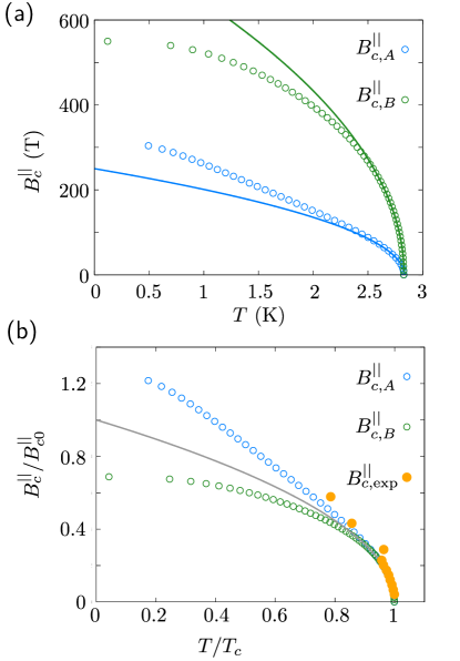
Figure 7: Temperature dependence of the critical magnetic field. (a) Open circles are the numerical results, solid lines are the fits to $B_{c}^{\scriptsize{||}}(T)=B_{c}^{\scriptsize{||}}(0)\,\sqrt{1-T/T_{c0}}$, where $T_{c0}$ is the critical temperature with $B_{\parallel}=0$. The prefactors are $B_{c,A}^{\scriptsize{||}}(0)=250$ T, $B_{c,B}^{\scriptsize{||}}(0)=800$ T. (b) Rescaled results, where the grey line is $\sqrt{1-T/T_{c0}}$, and orange points are digitized data from Fig. 4 in Ref. [Xi et al., 2016a].

On the one hand, both parametrizations display the expected behavior

$$B_{c}^{\scriptsize{||}}(T)=B_{c}^{\scriptsize{||}}(0)\,\sqrt{1-T/T_{c0}}$$ (74)

in the vicinity of the critical temperature at zero field, $T_{c0}$, in agreement with the experimental results Wan et al. (2021). On the other hand, the two sets $A$ and $B$ differ qualitatively as the temperature is decreased. Within the $A$ parametrization $B_{c}^{\scriptsize{||}}(T)$ displays almost a linear behavior at intermediate temperature, again in line with the experiment. The $B$ parametrization leads to much larger zero temperature critical fields than the $A$ one, and the scaled curve starts to deviate from the experimental data as the temperature decreases well below $T_{c}$.

V Conclusions

In summary, we have shown that two-bands superconductivity can naturally arise from repulsive interactions in NbSe₂. At its origin is the fragmentation of the Fermi surface, which features hole pockets around the time-reversal related $K$, $K^{\prime}$ points, as well as around the $\Gamma$ point. The latter, however, is not crucial for the effects discussed in this work where the superconductivity is driven by short-range intervalley scattering in combination with long-range intravalley interactions, for which two disjoint Fermi pockets are sufficient. Superconductivity induced by repulsive interactions which couple different valleys has been proposed for the iron pnictides Mazin (2010), bilayer graphene Guinea and Uchoa (2012), heavily doped MoS₂ Roldán et al. (2013), and recently also for NbSe₂ Shaffer et al. (2020). In our work we have extended in particular the treatment in Ref. [Roldán et al., 2013] to include the effects of Ising SOC and in-plane magnetic fields. For this purpose we have developed a fully microscopic approach based on a low energy, two-bands model for NbSe₂. The minimal model fits the hyperbolic dispersion for the holes near the $K$ and $K$’ valleys to the outcomes of a three $d$-orbital tight-binding model for TMDCs. For that purpose, two different tight-binding parametrizations for NbSe₂, called $A$ and $B$, are used. Due to the hyperbolic fit in combination with the Ising spin-orbit coupling, the two bands are gapped with two distinct gaps sharing the same critical temperature. As the temperature is decreased, the gaps at one valley acquire different size. Similar to conventional single gap BCS theory, we demonstrated a universal behavior of the average gap, when scaled by its zero temperature value, and with temperatures given in unit of the critical temperature. The temperature evolution of the scaled average gap matches the dataWan et al. (2021), which are compatible with the presence of two distinct gaps. At finite magnetic field the two bands are also gapped. Due to the breaking of time-reversal symmetry, the quasiparticle spectrum acquires an intricate dependence on various pairing contributions with different character upon momentum inversion. The investigation of the different phases that our theory predicts at finite magnetic field will, in particular in relation to the possible observation of triplet superconductivity in [Kuzmanović et al., 2021], be the object of our future work. Here rather we focused on the dependence of the critical in-plane magnetic field on temperature. A quantitative agreement with the scaled data in Ref. [Xi et al., 2016a] was found for one of the two chosen parametrizations, giving us confidence in the used microscopic low energy modeling.

Appendix A Diagonalization of the two bands superconducting Hamiltonian in finite in-plane magnetic field

In the following we provide a way to diagonalize the BdG Hamiltonian in Eq. (49). Notice that in this appendix, for ease of notation, we use the subscripts $1,2$ instead of $+,-$. Also, we are going to introduce several new quantities whose expression is listed at the very end of the section. Let us now consider the slightly more general case: Given $\tilde{\xi}_{1},\tilde{\xi}_{2}\in\mathbf{R}$ and $\Delta_{1},\Delta_{2},\Delta_{12}\in\mathbf{C}$, we wish to diagonalize the following hermitian matrix,

$$\mathcal{H}=\begin{pmatrix}\tilde{\xi}_{1}&0&\Delta_{1}&\Delta_{12}\\ 0&\tilde{\xi}_{2}&-\Delta_{12}&\Delta_{2}\\ \Delta_{1}^{*}&-\Delta^{*}_{12}&-\tilde{\xi}_{1}&0\\ \Delta^{*}_{12}&\Delta^{*}_{2}&0&-\tilde{\xi}_{2}\end{pmatrix}.$$ (75)

I.e., we look for the eigenvalues and the unitary transformation that leads to the diagonal form of $\mathcal{H}$. We start by first dividing the matrix into the two parts

$$\mathcal{H}=\mathcal{H}_{0}+\mathcal{H}_{12}=\begin{pmatrix}\tilde{\xi}_{1}&0&\Delta_{1}&0\\ 0&\tilde{\xi}_{2}&0&\Delta_{2}\\ \Delta_{1}^{*}&0&-\tilde{\xi}_{1}&0\\ 0&\Delta^{*}_{2}-&0&-\tilde{\xi}_{2}\end{pmatrix}+\begin{pmatrix}&&&\Delta_{12}\\ &&-\Delta_{12}&\\ &-\Delta^{*}_{12}&&\\ \Delta^{*}_{12}&&&\end{pmatrix}\,,$$ (76)

and proceed by diagonalizing just $\mathcal{H}_{0}$. Afterwards we express $\mathcal{H}_{12}$ in the eigenbasis of $\mathcal{H}_{0}$ to get to the matrix form of $\mathcal{H}$ in the new basis. Repeating this procedure eventually leads to a block diagonal matrix which can easily be diagonalized. The unitary transformation that diagonalizes $\mathcal{H}_{0}$ is rendered as

$$U_{0}=\begin{pmatrix}\Delta_{1}/\eta_{1}&0&-(E_{1}-\tilde{\xi}_{1})/\eta_{1}&0\\ 0&\Delta_{2}/\eta_{2}&0&-(E_{2}-\tilde{\xi}_{2})/\eta_{2}\\ (E_{1}-\tilde{\xi}_{1})/\eta_{1}&0&\Delta_{1}^{*}/\eta_{1}&0\\ 0&(E_{2}-\tilde{\xi}_{2})/\eta_{2}&0&\Delta_{2}^{*}/\eta_{2}\\ \end{pmatrix}\,,$$ (77)

where the values of the entries fulfill $(\Delta_{n}/\eta_{n})^{2}=\frac{1}{2}\left(1+\tilde{\xi}_{n}/E_{n}\right)$ and $[(E_{n}-\tilde{\xi}_{n})/\eta_{n}]^{2}=\frac{1}{2}\left(1-\tilde{\xi}_{n}/E_{n}\right)$. In the new basis, $\mathcal{H}$ reads

$$\tilde{\mathcal{H}}=U_{0}^{\dagger}\mathcal{H}U_{0}=\begin{pmatrix}E_{1}&&&\\ &E_{2}&&\\ &&-E_{1}&\\ &&&-E_{2}\\ \end{pmatrix}+\begin{pmatrix}0&Y&0&Z\\ Y^{*}&0&-Z&0\\ 0&-Z^{*}&0&Y^{*}\\ Z^{*}&0&Y&0\\ \end{pmatrix}\,.$$ (78)

Notice that

$$|Y|^{2}+|Z|^{2}=|\Delta_{12}|^{2}\,,\quad E_{1}E_{2}(|Y|^{2}-|Z|^{2})=4\tilde{\xi}_{1}\tilde{\xi}_{2}|\Delta_{12}|^{2}-\text{Re}(\Delta_{12}^{2}\Delta_{1}^{*}\Delta_{2}^{*})\,.$$ (79)

Even though the total number of entries is unchanged, we are now left with only two complex parameters $Y$ and $Z$ instead of the three provided by the gaps $\Delta_{1}$, $\Delta_{2}$ and $\Delta_{12}$ from before. In the second step we diagonalize the block diagonal part $\tilde{\mathcal{H}}_{Y}$ of $\tilde{\mathcal{H}}$; afterwards we express $\tilde{\mathcal{H}}_{Z}$, the off-diagonal matrix which contains the parameter $Z$, in the new eigenbasis. Here, the corresponding unitary transformation is given by

$$U_{1}=\dfrac{1}{\kappa_{1}}\begin{pmatrix}E_{2}-G_{1}&-Y&&\\ -Y^{*}&E_{2}-G_{1}&&\\ &&Y^{*}&E_{2}-G_{1}\\ &&E_{2}-G_{1}&Y\end{pmatrix}\,,$$ (80)

and we have the relation $(E_{2}-G_{1})=-(E_{1}-G_{2})$. In the new basis $\tilde{\mathcal{H}}$ looks like

$$K=U_{1}^{\dagger}\tilde{\mathcal{H}}U_{1}=\begin{pmatrix}G_{1}&&&\\ &G_{2}&&\\ &&-G_{2}&\\ &&&-G_{1}\\ \end{pmatrix}+\begin{pmatrix}&&R&S\\ &&T&-R\\ R^{*}&T^{*}&&\\ S^{*}&-R^{*}&&\\ \end{pmatrix}\,,$$ (81)

which appears to be in a very similar form as the matrix $\mathcal{H}$ we have started with. Notice, however, that we have the important relations $|S|^{2}=|T|^{2}$ and $TR^{*}=S^{*}R$. The latter is the reason why we get a block diagonal matrix after a final rotation. For this, we first consider the off-diagonal contribution $K_{R}$ of $K$ containing the $R$ elements. One finds the transformation

$$U_{2}=\dfrac{1}{\kappa_{2}}\begin{pmatrix}G_{2}+\tilde{G}_{1}&0&0&R\\ 0&R&-(G_{1}+\tilde{G}_{2})&0\\ R^{*}&0&0&-(G_{1}+\tilde{G}_{2})\\ 0&G_{2}+\tilde{G}_{1}&R^{*}&0\\ \end{pmatrix}$$ (82)

with the relation $G_{2}+\tilde{G}_{1}=G_{1}+\tilde{G}_{2}$. Performing the rotation now simply rearranges the entries $S$ and $T$ and we are left with the block diagonal matrix

$$\tilde{K}=U_{2}^{\dagger}KU_{2}=\begin{pmatrix}\tilde{G}_{1}&&&\\ &-\tilde{G}_{1}&&\\ &&\tilde{G}_{2}&\\ &&&-\tilde{G}_{2}\end{pmatrix}+\begin{pmatrix}0&S&&\\ S^{*}&0&&\\ &&0&T\\ &&T^{*}&0\\ \end{pmatrix}\,,$$ (83)

whose diagonalization is trivial and can now be done within one step. The fourth and last transformation assumes the form

$$U_{3}=\begin{pmatrix}(\tilde{G}_{1}+\tilde{E}_{1})/\lambda_{1}&0&S/\lambda_{1}&0\\ S^{*}/\lambda_{1}&0&-(\tilde{G}_{1}+\tilde{E}_{1})/\lambda_{1}&0\\ 0&(\tilde{G}_{2}+\tilde{E}_{2})/\lambda_{2}&0&T/\lambda_{2}\\ 0&T^{*}/\lambda_{2}&0&-(\tilde{G}_{2}+\tilde{E}_{2})/\lambda_{2}\end{pmatrix}$$ (84)

and finally gives

$$U_{3}^{\dagger}\tilde{K}U_{3}=\begin{pmatrix}\tilde{E}_{1}&&&\\ &\tilde{E}_{2}&&\\ &&-\tilde{E}_{1}&\\ &&&-\tilde{E}_{2}\end{pmatrix}\,.$$ (85)

Ultimately, the full unitary transformation, which diagonalizes the matrix $\mathcal{H}$ in Eq. (75), can be explicitly calculated from the product of all $U$’s. We conclude the diagonalization with

$$U=U_{0}U_{1}U_{2}U_{3}=\begin{pmatrix}u_{11}&u_{12}&u_{31}^{*}&-u_{32}^{*}\\ u_{21}&u_{22}&-u_{41}^{*}&u_{42}^{*}\\ u_{31}&u_{32}&-u_{11}^{*}&u_{12}^{*}\\ u_{41}&u_{42}&u_{21}^{*}&-u_{22}^{*}\\ \end{pmatrix}$$ (86)

where each entry has a very similar counterpart

$$\eta_{1}\kappa_{1}\kappa_{2}\lambda_{1}\cdot u_{11} =\Delta_{1}\left[(E_{2}-G_{1})(G_{2}+\tilde{G}_{1})(\tilde{G}_{1}+\tilde{E}_{1})-YRS^{*}\right]-(E_{1}-\tilde{\xi}_{1})\left[S^{*}(E_{2}-G_{1})(G_{2}+\tilde{G}{1})+Y^{*}R^{*}(\tilde{G}_{1}+\tilde{E}_{1})\right]\,,$$

$$\eta_{2}\kappa_{1}\kappa_{2}\lambda_{2}\cdot u_{22} =\Delta_{2}\left[(E_{2}-G_{1})(G_{2}+\tilde{G}_{1})(\tilde{G}_{2}+\tilde{E}_{2})-YRS^{*}\right]-(E_{2}-\tilde{\xi}_{2})\left[T^{*}(E_{2}-G_{1})(G_{2}+\tilde{G}{1})+YR^{*}(\tilde{G}_{2}+\tilde{E}_{2})\right]\,,$$

$$\eta_{1}\kappa_{1}\kappa_{2}\lambda_{2}\cdot u_{12} =\Delta_{1}\left[Y(G_{2}+\tilde{G}_{1})(\tilde{G}_{2}+\tilde{E}_{2})+RT^{*}(E_{2}-G_{1})\right]-(E_{1}-\tilde{\xi}_{1})\left[R^{*}(E_{2}-G_{1})(\tilde{G}_{2}+\tilde{E}_{2})-YS^{*}(G_{2}+\tilde{G}_{1})\right]\,,$$

$$-\eta_{2}\kappa_{1}\kappa_{2}\lambda_{1}\cdot u_{21} =\Delta_{2}\left[Y^{*}(G_{2}+\tilde{G}_{1})(\tilde{G}_{1}+\tilde{E}_{1})+RS^{*}(E_{2}-G_{1})\right]-(E_{2}-\tilde{\xi}_{2})\left[R^{*}(E_{2}-G_{1})(\tilde{G}_{1}+\tilde{E}_{1})-YS^{*}(G_{2}+\tilde{G}_{1})\right]\,,$$

$$\eta_{1}\kappa_{1}\kappa_{2}\lambda_{1}\cdot u_{31} =\Delta_{1}^{*}\left[S^{*}(E_{2}-G_{1})(G_{2}+\tilde{G}_{1})+Y^{*}R^{*}(\tilde{G}_{1}+\tilde{E}_{1})\right]+(E_{1}-\tilde{\xi}_{1})\left[(E_{2}-G_{1})(G_{2}+\tilde{G}_{1})(\tilde{G}_{1}+\tilde{E}_{1})-YRS^{*}\right]\,$$

$$\eta_{2}\kappa_{1}\kappa_{2}\lambda_{2}\cdot u_{42} =\Delta_{2}^{*}\left[T^{*}(E_{2}-G_{1})(G_{2}+\tilde{G}_{1})+YR^{*}(\tilde{G}_{2}+\tilde{E}_{2})\right]+(E_{2}-\tilde{\xi}_{2})\left[(E_{2}-G_{1})(G_{2}+\tilde{G}_{1})(\tilde{G}_{2}+\tilde{E}_{2})-YRS^{*}\right]\,$$

$$\eta_{1}\kappa_{1}\kappa_{2}\lambda_{2}\cdot u_{32} =\Delta_{1}^{*}\left[R^{*}(E_{2}-G_{1})(\tilde{G}_{2}+\tilde{E}_{2})-YS^{*}(G_{2}+\tilde{G}_{1})\right]+(E_{1}-\tilde{\xi}_{1})\left[Y(G_{2}+\tilde{G}_{1})(\tilde{G}_{2}+\tilde{E}_{2})+RT^{*}(E_{2}-G_{1})\right]\,,$$

$$-\eta_{2}\kappa_{1}\kappa_{2}\lambda_{1}\cdot u_{41} =\Delta_{2}^{*}\left[R^{*}(E_{2}-G_{1})(\tilde{G}_{1}+\tilde{E}_{1})-YS^{*}(G_{2}+\tilde{G}_{1})\right]+(E_{2}-\tilde{\xi}_{2})\left[Y^{*}(G_{2}+\tilde{G}_{1})(\tilde{G}_{1}+\tilde{E}_{1})+RS^{*}(E_{2}-G_{1})\right]\,,$$

and where we used $Y^{*}S=YT$. Further using the relations Eq. (79) leads to the explicit form of the eigenvalues. They read

$$\tilde{E}_{n} =\dfrac{1}{\sqrt{2}}\sqrt{E_{1}^{2}+E_{2}^{2}+2|\Delta_{12}|^{2}\pm\sqrt{\left(E_{1}^{2}-E_{2}^{2}\right)^{2}+4|\Delta_{12}|^{2}\left[\left(\tilde{\xi}_{1}+\tilde{\xi}_{2}\right)^{2}+|\Delta_{1}|^{2}+|\Delta_{2}|^{2}\right]-8\text{Re}\left(\Delta_{12}^{2}\Delta_{1}^{*}\Delta_{2}^{*}\right)}}\,.$$ (87)

The transformation $U$, however, is still only given in an implicit form where each of our introduced abbreviations appear.

The list below shows the abbreviations introduced in the diagonalization process. Here, each block corresponds to the quantities that appear in one of the transformations $U_{i}$ and in the transformed matrix upon applying this transformation.

$$I.\quad E_{n} =\sqrt{\tilde{\xi}_{n}^{2}+|\Delta_{n}|^{2}} Y =\dfrac{1}{\eta_{1}\eta_{2}}\left[\Delta_{12}\Delta_{1}^{*}\left(E_{2}-\tilde{\xi}_{2}\right)-\Delta_{12}^{*}\Delta_{2}\left(E_{1}-\tilde{\xi}_{1}\right)\right]$$

$$\eta_{n} =\sqrt{2E_{n}\left(E_{n}-\tilde{\xi}_{n}\right)} Z =\dfrac{1}{\eta_{1}\eta_{2}}\left[\Delta_{12}\Delta_{1}^{*}\Delta_{2}^{*}+\Delta_{12}^{*}\left(E_{1}-\tilde{\xi}_{1}\right)\left(E_{2}-\tilde{\xi}_{2}\right)\right]$$

$$II.\quad G_{n} =\dfrac{1}{2}\left[\left(E_{1}+E_{2}\right)\pm\sqrt{\left(E_{1}+E_{2}\right)^{2}+4|Y|^{2}}\right] \quad R =\dfrac{1}{\kappa_{1}^{2}}Z\left[|Y|^{2}-\left(E_{2}-G_{1}\right)^{2}\right]$$

$$\kappa_{1} =\sqrt{\left(E_{2}-G_{1}\right)^{2}+|Y|^{2}} S =\dfrac{2}{\kappa_{1}^{2}}YZ\left(E_{1}-G_{1}\right)$$

$$T =\dfrac{2}{\kappa_{1}^{2}}Y^{*}Z\left(E_{2}-G_{1}\right)$$

$$III.\quad \tilde{G}_{n} =\pm\dfrac{1}{2}\left[\left(G_{1}-G_{2}\right)\pm\sqrt{\left(G_{1}+G_{2}\right)^{2}+4|R|^{2}}\right] \kappa_{-} =\sqrt{\left(G_{2}-\tilde{G}_{1}\right)^{2}+|R|^{2}}$$

$$IV.\quad \tilde{E}_{n} =\sqrt{\tilde{G}_{n}^{2}+|S|^{2}} \lambda_{n} =\sqrt{\left(\tilde{G}_{n}+\tilde{E}_{n}\right)^{2}+|S|^{2}}$$

References

- Kohn and Luttinger (1965) W. Kohn and J. M. Luttinger, Phys. Rev. Lett. 15, 524 (1965), URL https://link.aps.org/doi/10.1103/PhysRevLett.15.524.
- Mazin (2010) I. I. Mazin, Nature 464, 183 (2010), URL https://www.nature.com/articles/nature08914.
- Qui et al. (2021) D. Qui, C. Gong, S. Wang, M. Zhang, C. Yang, X. Wang, and J. Xiong, Advanced Materials 499, 419 (2021), URL https://onlinelibrary.wiley.com/doi/abs/10.1002/adma.202006124.
- Taniguchi et al. (2012) K. Taniguchi, A. Matsumoto, H. Shimotani, and H. Tagaki, Appl. Phys. Lett. 101, 042603 (2012), URL https://aip.scitation.org/doi/10.1063/1.4740268.
- Ye et al. (2012) J. T. Ye, Y. J. Zhang, R. Akashi, M. S. Bahramy, R. Arita, and Y. Iwasa, Science 338, 1193 (2012), URL https://www.science.org/doi/10.1126/science.1228006.
- Saito et al. (2016) Y. Saito, Y. Nakamura, M. S. Bahramy, Y. Kohama, J. Ye, Y. Kasahara, Y. Nakagawa, M. Onga, M. Tokunaga, T. Nojima, et al., Nature Physics 12, 144 (2016), URL https://doi.org/10.1038/nphys3580.
- Roldán et al. (2013) R. Roldán, E. Cappelluti, and F. Guinea, Phys. Rev. B 88, 054515 (2013), URL https://link.aps.org/doi/10.1103/PhysRevB.88.054515.
- N.F.Q. Yuan and Law (2014) K. M. N.F.Q. Yuan and K. Law, Phys. Rev. Lett. 113, 097001 (2014), URL https://journals.aps.org/prl/abstract/10.1103/PhysRevLett.113.097001.
- Hsu et al. (2017) Y.-T. Hsu, A. Vaezi, M. H. Fischer, and E.-A. Kim, Nano Lett. 8, 14985 (2017), URL https://www.nature.com/articles/ncomms14985.
- Oiwa et al. (2018) R. Oiwa, Y. Yanagi, and H. Kusunose, Phys. Rev. B 98, 064509 (2018), URL https://journals.aps.org/prb/abstract/10.1103/PhysRevB.98.064509.
- Xi et al. (2016a) X. Xi, Z. Wang, W. Zhao, J.-H. Park, K. Law, H. Berger, L. Forró, J. Shan, and K. Mak, Nature Physics 12, 139 (2016a), URL https://doi.org/10.1038/nphys3538.
- Shaffer et al. (2020) D. Shaffer, J. Kang, F. J. Burnell, and R. M. Fernandes, Phys. Rev. B 101, 224503 (2020), URL https://link.aps.org/doi/10.1103/PhysRevB.101.224503.
- Zhou et al. (2016) B. T. Zhou, N. F. Q. Yuan, H.-L. Jiang, and K. T. Law, Phys. Rev. B 93, 180501 (2016), URL https://link.aps.org/doi/10.1103/PhysRevB.93.180501.
- Ilić et al. (2017) S. Ilić, J. S. Meyer, and M. Houzet, Phys. Rev. Lett. 119, 117001 (2017), URL https://link.aps.org/doi/10.1103/PhysRevLett.119.117001.
- Möckli and Khodas (2018) D. Möckli and M. Khodas, Phys. Rev. B 98, 144518 (2018), URL https://link.aps.org/doi/10.1103/PhysRevB.98.144518.
- Tang et al. (2021) G. Tang, C. Bruder, and W. Belzig, Phys. Rev. Lett. 126, 237001 (2021), URL https://journals.aps.org/prl/abstract/10.1103/PhysRevLett.126.237001.
- Ugeda et al. (2016) M. M. Ugeda, A. J. Bradley, Y. Zhang, S. Onishi, Y. Chen, W. Ruan, C. Ojeda-Aristizabal, H. Ryu, M. T. Edmonds, H.-Z. Tsai, et al., Nature Physics 12, 92 (2016), URL https://www.nature.com/articles/nphys3527.
- Y. Xing et al. (2017) Y. Xing et al. , Nano Lett. 17, 6802 (2017), URL https://pubs.acs.org/doi/10.1021/acs.nanolett.7b03026.
- et al. (2018) E. K. et al., Nanol Lett. 18, 2623 (2018), URL https://pubs.acs.org/doi/10.1021/acs.nanolett.8b00443.
- et al. (2021) A. H. et al., Nature Phys. 17, 949 (2021), URL https://www.nature.com/articles/s41567-021-01219-x.
- Kuzmanović et al. (2021) M. Kuzmanović, T. Dvir, D. LeBoeuf, S. Ilić, D. Möckli, M. Haim, S. Kraemer, M. Khodas, M. Houzet, J. S. Meyer, et al. (2021), eprint https://doi.org/10.48550/arXiv.2104.00328, URL https://doi.org/10.48550/arXiv.2104.00328.
- K. Zhao et al. (2019) K. Zhao et al. , Nature Phys. 17, 6802 (2019), URL https://www.nature.com/articles/s41567-019-0570-0.
- Wan et al. (2021) W. Wan, P. Dreher, D. Muñoz-Segovia, R. Harsh, F. Guinea, F. de Juan, and M. M. Ugeda (2021), eprint arXiv2101.04050, URL https://arxiv.org/abs/2101.04050.
- Geim and Grigorieva (2013) A. K. Geim and I. V. Grigorieva, Nature 499, 419 (2013), URL https://www.nature.com/articles/nature12385.
- Xi et al. (2016b) X. Xi, H. Berger, L. Forró, J. Shan, and K. F. Mak, Phys. Rev. Lett. 117, 106801 (2016b), URL https://link.aps.org/doi/10.1103/PhysRevLett.117.106801.
- Liu et al. (2013) G.-B. Liu, W.-Y. Shan, Y. Yao, W. Yao, and D. Xiao, Phys. Rev. B 88, 085433 (2013), URL https://journals.aps.org/prb/abstract/10.1103/PhysRevB.88.085433.
- Kim and Son (2017) S. Kim and Y.-W. Son, Phys. Rev. B 96, 155439 (2017), URL https://link.aps.org/doi/10.1103/PhysRevB.96.155439.
- He et al. (2018) W.-Y. He, B. T. Zhou, J. J. He, N. F. Q. Yuan, T. Zhang, and K. T. Law, Communications Physics 1, 40 (2018), URL https://doi.org/10.1038/s42005-018-0041-4.
- Valla et al. (2004) T. Valla, A. Fedorov, P. Johnson, P.-A. Glans, C. McGuinness, K. E. Smith, E. Y. Andrei, and H. Berger, Phys. Rev. Lett. 92, 086401 (2004), URL https://journals.aps.org/prl/abstract/10.1103/PhysRevLett.92.086401.
- Noat et al. (2015) Y. Noat, J. A. Silva-Guillén, T. Cren, V. Cherkez, C. Brun, S. Pons, F. Debontridder, D. Roditchev, W. Sacks, L. Cario, et al., Phys. Rev. B 92, 134510 (2015), URL https://link.aps.org/doi/10.1103/PhysRevB.92.134510.
- Heil et al. (2017) C. Heil, H. Berger, S. Poncé, H. Lambert, M. Schlipf, E. R. Margine, and F. Giustino, Phys. Rev. Lett. 119, 087003 (2017), URL https://journals.aps.org/prl/abstract/10.1103/PhysRevLett.119.087003.
- Sanna et al. (2022) A. Sanna, C. Pellegrini, E. Liebhaber, K. Rossnagel, J. K. Franke, and E. K. U. Gross, npj Quantum Materials 7, 6 (2022), URL https://www.nature.com/articles/s41535-021-00412-8.
- Bardeen et al. (1957) J. Bardeen, L. N. Cooper, and J. R. Schrieffer, Phys. Rev. 108, 1175 (1957), URL https://journals.aps.org/pr/references/10.1103/PhysRev.108.1175.
- Guinea and Uchoa (2012) F. Guinea and B. Uchoa, Phys. Rev. B 86, 134521 (2012), URL https://journals.aps.org/prb/pdf/10.1103/PhysRevB.86.134521.
- not (a) The polynomial yields two real solutions and hence also two different values for . This other value can be obtained by simply changing the sign in front of the root. However, the resulting leads to a contradiction with the assumption and is hence discarded.
- Dvir et al. (2018) T. Dvir, F. Massee, L. Attias, M. Khodas, M. Aprili, C. H. L. Quay, and H. Steinberg, Nature Communications 9, 598 (2018), URL https://www.nature.com/articles/s41467-018-03000-w.
- Tinkham (2004) M. Tinkham, Introduction to superconductivity (2nd ed.) (Dover Publications, 2004).
- Black-Schaffer and Honerkamp (2014) A. M. Black-Schaffer and C. Honerkamp, J. Phys.: Cond. Mat. 26, 423201 (2014), URL https://iopscience.iop.org/article/10.1088/0953-8984/26/42/423201.
- not (b) Since in our diagonalization process, the Hamiltonian assumes a diagonal form already after the first step. All of the introduced eigenenergies there will then reduce to which is simply the one from Eq. (15). Further, the products appearing in the functions will vanish because every term in them is either multiplied by or . The products in on the other side reduce to .
- not (c) The problematic factors are the introduced in the diagonalization which have to be paired with either or . Setting then both to zero will lead to a finite result (cf. Eq. (77)).