Arithmeticity of the Kontsevich–Zorich monodromies of certain families of square-tiled surfaces

Abstract.

The variations of Hodge structures of weight one associated to square-tiled surfaces naturally generate interesting subgroups of integral symplectic matrices called Kontsevich–Zorich monodromies. In this paper, we show that arithmetic groups are frequent among the Kontsevich–Zorich monodromies of square-tiled surfaces of low genera $g$.

1. Introduction

A subgroup $\Gamma\subset GL(n,\mathbb{Z})$ with Zariski closure $G$ is called arithmetic, resp., thin (in the sense of Sarnak [36]) if the index of $\Gamma$ in $G(\mathbb{Z})$ is finite, resp. infinite. From the point of view of Number Theory, the problems driven by thin matrix groups possess an “extra” degree of difficulty in comparison with the questions involving arithmetic matrix groups. Partly motivated by this fact, several authors tried to identify how often one meets thin matrix groups in certain geometric situations: for example,

• certain Calabi–Yau threefolds form 14 families whose moduli spaces are isomorphic to $\overline{\mathbb{C}}\setminus\{0,1,\infty\}$, so that one gets 14 examples of subgroups of $\textrm{Sp}(4,\mathbb{Z})$ (with full Zariski closures) by looking at the corresponding variations of Hodge structures; in this context, Brav and Thomas [5] showed that 7 families lead to thin matrix groups, and Singh and Venkataramana [38], [39] proved that the remaining 7 families lead to arithmetic groups;

• the setting of the previous paragraph can be significantly extended by looking at the monodromy groups generated by hypergeometric differential equations, and, in this direction, many new examples of thin matrix groups were found by Fuchs, Meiri and Sarnak [16], Filip and Fougeron [15], [12], among other authors.

In this paper, we are interested in the Kontsevich–Zorich monodromies of square-tiled surfaces, i.e., the matrix groups associated to the actions on the first homology groups of affine homeomorphisms of square-tiled surfaces or, equivalently, the variations of Hodge structures along the closed $\operatorname{SL}(2,\mathbb{R})$-orbits spanned by integral points in moduli spaces of translation surfaces. In this direction, we don’t have examples of thin Kontsevich–Zorich monodromies with the largest possible Zariski closures (despite a recent effort by Hubert–Matheus [22]), and, in fact, our two main results below partly explain why it might not be easy to find such examples among square-tiled surfaces of genera three and four with a single conical singularity.

Theorem 1.

There are infinitely many square-tiled surfaces of genus three with a single conical singularity whose Kontsevich–Zorich monodromies are arithmetic.

In particular, conditionally on a conjecture by Delecroix and Lelièvre (whose statement is recalled in the next section), this theorem says that a positive proportion (at least $1/8$) of the $SL(2,\mathbb{R})$-orbits of square-tiled surfaces of genus three with a single conical singularity have arithmetic KZ monodromies: for more precise formulations of Theorem 1, see the statements of Theorems 5, 6 and 9 below.

Theorem 2.

For each $10\leq n\leq 260$ which is divisible by $5$, there exists a square-tiled surface of genus four with a single conical singularity tiled by $n$ squares whose Kontsevich–Zorich monodromy is arithmetic.

The proof of these results occupy the remainder of this article. More concretely, we quickly review in Section 2 the aspects of the theory of square-tiled surfaces entering into the statements of Theorems 1 and 2, and the relevant strategy towards the arithmeticity of subgroups of symplectic matrices. After that, in Section 3, we prove two results, namely Theorems 5 and 6, yielding a precise version of Theorem 1 in the context of the so-called odd component of $\mathcal{H}(4)$. Subsequently, we complete in Section 4 the discussion of Theorem 1 by showing a statement, namely Theorem 9, giving a precise version of Theorem 1 in the context of the so-called hyperelliptic component of $\mathcal{H}(4)$. Next, we establish Theorem 2 in Section 5. Once the main result are proved, we include in Section 6 some numerical experiments about the indices of the KZ monodromies (in the integral lattices in their Zariski closures) of some square-tiled surfaces in genus two and we describe two curious examples in genera three and four: in particular, concerning the genus two case, the list of such indices seems to take only two values ($1$ or $3$) for square-tiled surfaces in $\mathcal{H}(2)$, while many values (including $1$, $3$, $4$, $6$, $12$, $24$) seem to be taken for square-tiled surfaces in $\mathcal{H}(1,1)$. Finally, we complete the article with two appendices: in Appendix A, we briefly compute the KZ monodromy of a square-tiled surface of genus three in the Prym locus (but unfortunately we are not able to infer whether arithmeticity or thinness should be typically expected in this special locus of $\mathcal{H}^{odd}(4)$), and in Appendix B, we explain the result of Möller that the KZ monodromy of any square-tiled surface of genus 2 is always arithmetic.

Acknowledgments

We thank Martin Möller for allowing us to include his unpublished result about the arithmeticity of the KZ monodromy of square-tiled surfaces of genus 2 in Appendix B and for his helpful and unwavering support. R. Niño would like to thank CONACYT’s Ph.d. grant. M. Sedano would like to thank UNAM-DGAPA’s posdoctoral grant. F.Valdez would like to thank the following grants: CONACYT Ciencia Básica CB-2016 283960 and UNAM PAPIIT IN-101422. The working group of G. Weitze-Schmithüsen is funded by the Deutsche Forschungsgemeinschaft (DFG, German Research Foundation) – Project-ID 286237555 – TRR 195.

2. Preliminaries

Recall that a square-tiled surface (or origami) is a pair $(M,\omega)$, where $M$ is a compact Riemann surface obtained from a ramified covering $\pi:M\to\mathbb{T}^{2}$ of the flat torus $\mathbb{T}^{2}=\mathbb{C}/(\mathbb{Z}\oplus i\mathbb{Z})$ which is not branched outside $0\in\mathbb{T}^{2}$, and $\omega$ is the Abelian differential given by pullback under $\pi$ of $dz$ on $\mathbb{T}^{2}$. In the sequel, we shall assume that our square-tiled surfaces are reduced in the sense that the group of relative periods of $\omega$ is $\mathbb{Z}\oplus i\mathbb{Z}$, and we refer the reader to [29] for more explanations about the basic features of square-tiled surfaces.

2.1. Kontsevich–Zorich monodromy of origamis

An affine homeomorphism $A$ of a reduced square-tiled surface $(M,\omega)$ is an orientation-preserving homeomorphism of $M$ given by affine maps in the local charts obtained from the local primitives of $\omega$ outside its zeroes. In this situation, the linear part $DA$ of $A$ is an element of $SL(2,\mathbb{Z})$, and the finite-index subgroup of $SL(2,\mathbb{Z})$ consisting of all linear parts of all affine homeomorphisms of $(M,\omega)$ is called the Veech group of $(M,\omega)$.

The first homology group $H_{1}(M,\mathbb{Q})$ of a reduced origami has a splitting

$$H_{1}(M,\mathbb{Q})=H_{1}^{st}(M,\mathbb{Q})\oplus H_{1}^{(0)}(M,\mathbb{Q})$$

which is respected by the natural action of the affine homeomorphisms of $(M,\omega)$. In concrete terms, $H_{1}^{(0)}(M,\mathbb{Q})$ is the kernel of $\pi_{*}:H_{1}(M,\mathbb{Q})\to H_{1}(\mathbb{T}^{2},\mathbb{Q})$, and $H_{1}^{st}(M,\mathbb{Q})$ is the orthogonal complement of $H_{1}^{(0)}(M,\mathbb{Q})$ with respect to the symplectic intersection form $\Omega$ on $H_{1}(M,\mathbb{Q})$. Each square in an origami defines two relative cycles $h_{i}$ and $v_{i}$ given by the bottom horizontal and left vertical sides respectively. These cycles define a base for $H_{1}^{st}(M,\mathbb{Q})$ given by $\sigma=\sum_{i}h_{i}$ and $\xi=\sum_{i}v_{i}$. In our cases the elements $h_{i}$ and $v_{i}$ also define a base for $H_{1}(M,\mathbb{Q})$ and $H_{1}^{(0)}(M,\mathbb{Q})$. In the first space each element of a base is given by $\sigma_{m}=\sum h_{i_{l}}$ and $\xi_{k}=\sum v_{i_{p}}$, for some subsets of indices $l$ and $p$. For the latter space the elements of a base are of the form $\sigma_{i}-\lambda\sigma_{j}$ and $\xi_{r}-\kappa\xi_{s}$, for some $i\neq j,r\neq s$ and $\lambda,\kappa\neq 0$.

An affine homeomorphism $A$ of $(M,\omega)$ acts on $H_{1}^{st}(M,\mathbb{Q})\simeq\mathbb{Q}^{2}$ via the linear action of $DA\in\textrm{SL}(2,\mathbb{Z})$ on $\mathbb{Q}^{2}$, and the subgroup of $\textrm{Sp}(H_{1}^{(0)}(M,\mathbb{Z}))\simeq\textrm{Sp}_{\Omega}(2g-2,\mathbb{Z})$ generated by the actions on $H_{1}^{(0)}(M,\mathbb{Q})$ of all affine homeomorphisms of $(M,\omega)$ is called the Kontsevich–Zorich monodromy / shadow Veech group of $(M,\omega)$.

An origami $(M,\omega)$ has arithmetic, resp. thin Kontsevich–Zorich (KZ) monodromy (in the sense of Sarnak [36]) if its KZ monodromy has finite, resp. infinite index in $G(\mathbb{Z})$, where $G$ is the Zariski closure of its KZ monodromy.

2.2. Zariski denseness in symplectic groups

Let $\Omega$ be a symplectic form on $\mathbb{Q}^{2d}$ taking integral values on the lattice $\mathbb{Z}^{2d}$. A matrix $A\in\textrm{Sp}_{\Omega}(2d,\mathbb{Z})$ is called Galois-pinching whenever its characteristic polynomial is irreducible over $\mathbb{Q}$, its roots are all real, and its Galois group is the largest possible (namely, isomorphic to the hyperoctahedral group of order $2^{d}\cdot d!$ viewed as the centralizer of the involution $\lambda\to\lambda^{-1}$ on the set of roots).

The Zariski closure of a subgroup $\Gamma\subset\textrm{Sp}_{\Omega}(2d,\mathbb{Z})$ containing a Galois-pinching matrix $A$ and an infinite order matrix $B$ not commuting with $A$ is $\textrm{Sp}_{\Omega}(2d,\mathbb{R})$ or isomorphic to $\textrm{SL}(2,\mathbb{R})^{d}$ after Prasad and Rapinchuk (cf. [34, Theorem 9.10]). After a conjugation of matrices, the subgroup $\textrm{SL}(2,\mathbb{R})^{d}$ is a block-diagonal group and in particular, preserves a decomposition $\mathbb{R}^{2}\oplus\cdots\oplus\mathbb{R}^{2}\cong\mathbb{R}^{2d}$. Thus, by combining this fact with [29, Prop. 4.3], we deduce that if $\Gamma\subset\textrm{Sp}_{\Omega}(2d,\mathbb{Z})$ containing a Galois-pinching matrix $A$ and an unipotent matrix $B\neq Id$ such that $(B-Id)(\mathbb{R}^{2d})$ is not a Lagrangian subspace, then $\Gamma$ is Zariski dense in $\textrm{Sp}_{\Omega}(2d,\mathbb{R})$. A particular case where this happens is when $(B-Id)(\mathbb{R}^{2d})$ has a dimension different from $d$, which is the dimension of a Lagrangian subspace.

The Galois-pinching property of a matrix $A\in\textrm{Sp}_{\Omega}(4,\mathbb{Z})$ with characteristic polynomial $x^{4}+ax^{3}+bx^{2}+ax+1\in\mathbb{Z}[x]$ can be directly checked with the help of three discriminants: more precisely, $A$ is Galois-pinching whenever $-a-4>0$, $b+2a+2>0$, and the discriminants $\Delta_{1}=a^{2}-4b+8>0$, $\Delta_{2}=(b+2+2a)(b+2-2a)$ and $\Delta_{1}\Delta_{2}$ are not squares (cf. [29, §6.7]).

2.3. Arithmeticity of subgroups of symplectic matrices

Let $\Omega$ be a symplectic form on $\mathbb{Q}^{2d}$ taking integral values on the lattice $\mathbb{Z}^{2d}$. Suppose that $\Gamma\subset Sp_{\Omega}(2d,\mathbb{Z})$ is Zariski dense and there are three transvections $T_{n}\in\Gamma$, $n=1,2,3$, such that $(T_{n}-\textrm{Id})(\mathbb{Z}^{2d})=\mathbb{Z}w_{n}$ satisfies $\Omega(w_{1},w_{2})\neq 0$. In this setting, Singh and Venkataramana showed that $\Gamma$ is arithmetic if the group generated by the restrictions of $T_{n}$ to $W=\mathbb{Q}w_{1}\oplus\mathbb{Q}w_{2}\oplus\mathbb{Q}w_{3}$ contains an element of the unipotent radical of $Sp_{\Omega}(W)$ (cf. [39, Theorem 1.2]).

A three-dimensional vector space with a non-trivial alternating form as above has a null space generated by an element $\langle e\rangle\leq W$, so that $\{e,w_{1},w_{2}\}$ is a basis of $W$. In such basis, the symplectic group is described as

$$Sp(W)=\left\{\left(\begin{array}[]{ccc}\lambda&x&y\\ 0&a&b\\ 0&c&d\end{array}\right)\in GL_{3}(\mathbb{Q}):\lambda\neq 0,\ ad-bc=1\right\}\cong(\mathbb{Q}^{*}\times SL_{2}(\mathbb{Q}))\ltimes\mathbb{Q}^{2}.$$

As $Sp(2,\mathbb{Q})=SL_{2}(\mathbb{Q})$ is a simple factor, the radical subgroup of $Sp(W)$, being the greatest normal, solvable subgroup, is

$$R(Sp(W))=\left\{\left(\begin{array}[]{ccc}\lambda&x&y\\ 0&1&0\\ 0&0&1\end{array}\right)\in GL_{3}(\mathbb{Q}):\lambda\neq 0\right\}\cong\mathbb{Q}^{*}\ltimes\mathbb{Q}^{2}$$

and the unipotent radical is

$$U(Sp(W))=\left\{\left(\begin{array}[]{ccc}1&x&y\\ 0&1&0\\ 0&0&1\end{array}\right)\in GL_{3}(\mathbb{Q}):\right\}\cong\mathbb{Q}^{2}.$$

However, we will be dealing with symplectic matrices $A\in Sp_{\Omega}(2d,\mathbb{Z})$ which preserve the element $e$, so their restriction lies in the subgroup

$$\left\{\left(\begin{array}[]{ccc}1&x&y\\ 0&a&b\\ 0&c&d\end{array}\right)\in GL_{3}(\mathbb{Q}):\lambda\neq 0,\ ad-bc=1\right\}\cong SL_{2}(\mathbb{Q})\ltimes\mathbb{Q}^{2}.$$

This is a small error made in [39], where they stated that in fact $Sp(W)\cong SL_{2}(\mathbb{Q})\ltimes\mathbb{Q}^{2}$. This is a harmless error, because it doesn’t affect their result, as they were also considering elements fixing the element $e$.

Remark 3.

Interestingly enough, Singh and Venkataramana also discuss in [39, §2] an alternative arithmeticity criterion closer to a recent work of Benoist and Miquel [1] which was used by Hubert and Matheus [22] to establish the arithmeticity of the KZ monodromy of a specific example origami of genus $3$. However, it seems hard to push this method to produce infinite families of examples of arithmetic KZ monodromies.

2.4. 2-cylinder decomposition and transvections in $\mathcal{H}(4)$

For each direction $\theta$ decomposing an origami in $\mathcal{H}(4)$ into 2 cylinders, we can associate an affine multitwist acting on $H_{1}^{(0)}(M,\mathbb{Q})$ as a transvection. We explain this in what follows.

Recall that the moduli of a cylinder $C$ is the quotient of $height(C)$ by $circumference(C)$. If in some direction the translation flow decomposes $M$ into a cylinders $C_{i}$ whose moduli $\mu_{i}$ satisfies $\mu_{i}=\frac{n_{i}}{\lambda}$ (i.e. these moduli are commensurable) then there exists a unique affine automorphism $D$ of $M$ that fixes the boudaries of these cylinders and has derivative (modulo conjugation) $\left(\begin{smallmatrix}1&\lambda\\ 0&1\end{smallmatrix}\right)$.

In an origami, every cylinder decomposition presents cylinders of commensurable moduli. Let us denote by $D$ the affine automorphism of an origami $M\in\mathcal{H}(4)$ associated to the 2-cylinder direction $\theta$. The action of $D$ on $H_{1}(M,\mathbb{Q})$ is given by:

$$D_{*}=I+c_{1}f_{2}\Omega(\cdot,\gamma_{1})\gamma_{1}+c_{2}f_{1}\Omega(\cdot,\gamma_{2})\gamma_{2}.$$ (2.1)

where $c_{i},f_{i}\in\mathbb{Q}$ are constants coming from the geometry of the cylinder decomposition in question. More precisely, if $\gamma_{1}$ and $\gamma_{2}$ are the core curves of the cylinders in the decomposition then $\pi_{*}(\gamma_{1})=f_{1}\pi(\gamma_{1})$ and $\pi_{*}(\gamma_{2})=f_{2}\pi(\gamma_{2})$. The constants $c_{i}$ are related also to the heights and the widths of the cylinders. For instance, if $\omega_{1}=m\omega_{2}$, (here $\omega_{1}$ and $\omega_{2}$ are the widths of the cylinders of $\gamma_{1}$ and $\gamma_{2}$, respectively) for $m\in\mathbb{N}$ then $c_{1}=m$ and $c_{2}=1$. Remark that for every $\beta\in H_{1}^{(0)}(M,\mathbb{Q})$, $c_{1}\Omega(\beta,\gamma_{1})=-c_{2}\Omega(\beta,\gamma_{2})$, and thus, if $X=f_{2}\gamma_{1}-f_{1}\gamma_{2}$ we have that the restriction of $D_{*}$ to $H_{1}^{(0)}(M,\mathbb{Q})$, which we denote $D_{X}$, is given by the transvection:

$$D_{X}=I+c\Omega(\cdot,X)X$$ (2.2)

for some $c\in\mathbb{Q}$.

2.5. Origamis in $\mathcal{H}(4)$

The moduli space of translation surfaces $(M,\omega)$ of compact Riemann surfaces $M$ of genus $3$ equipped with Abelian differentials $\omega$ possessing a single zero (of order four) is denoted by $\mathcal{H}(4)$. After Kontsevich and Zorich [26], $\mathcal{H}(4)$ has two connected components $\mathcal{H}^{hyp}(4)$ and $\mathcal{H}^{odd}(4)$, and $(M,\omega)\in\mathcal{H}(4)$ belongs to $\mathcal{H}^{hyp}(4)$ if and only if it admits an affine homeomorphism with linear part $-Id$, i.e., an anti-automorphism, possessing eight fixed points. An origami $(M,\omega)\in\mathcal{H}^{odd}(4)$ may also possess an anti-automorphism (with four fixed points): in this case, we say that it belongs to the Prym locus of $\mathcal{H}^{odd}(4)$.

2.5.1. $SL(2,\mathbb{Z})$-orbits in $\mathcal{H}(4)$ and their invariants

Recall that the subset of origamis can be organized into $SL(2,\mathbb{Z})$-orbits: indeed, any origami $(M,\pi^{*}(dz))$, $\pi:M\to\mathbb{T}^{2}$, is coded by a pair of permutations $(h,v)\in S_{N}\times S_{N}$, where $N$ is the degree of $\pi$, modulo simultaneous permutations (i.e., $(h,v)\equiv(\phi h\phi^{-1},\phi v\phi^{-1})$), and the usual parabolic generators of $SL(2,\mathbb{Z})$ act on pairs of permutations via the Nielsen transformations $(h,v)\mapsto(h,vh^{-1})$ and $(h,v)\mapsto(hv^{-1},v)$.

From the discussion in the previous paragraph, it is clear that the isomorphism class of the group $G=\langle h,v\rangle\subset S_{N}$ generated by a pair of permutations $(h,v)$ coding an origami $(M,\omega)$ is an invariant of its $SL(2,\mathbb{Z})$-orbit. This isomorphism class is called the monodromy of $(M,\omega)$. As it was shown by Zmiaikou (see also [29, Prop. 6.1 and 6.2]), the monodromy of any reduced origami $(M,\omega)\in\mathcal{H}(4)$ is $A_{N}$ or $S_{N}$ whenever the degree of $\pi:M\to\mathbb{T}^{2}$ is $N\geq 7$.

If a reduced origami $(M,\omega)\in\mathcal{H}(4)$ possesses an anti-automorphism $\iota$, then the fixed points of $\iota$ project under $\pi$ on the $2$-torsion (half-integer) points of $\mathbb{T}^{2}$, and we can produce a list $(l_{0},[l_{1},l_{2},l_{3}])$ where $l_{0}=\#(\textrm{Fix}(\iota)\cap\pi^{-1}(0))-1$, $l_{1}=\#(\textrm{Fix}(\iota)\cap\pi^{-1}(1/2))$, $l_{2}=\#(\textrm{Fix}(\iota)\cap\pi^{-1}(i/2))$, and $l_{3}=\#(\textrm{Fix}(\iota)\cap\pi^{-1}((1+i)/2))$, where $[l_{1},l_{2},l_{3}]$ stands for an unordered triple. Since $SL(2,\mathbb{Z})$ acts on $\mathbb{T}^{2}$ by fixing $0\in\mathbb{T}^{2}$ and permuting the other three $2$-torsion points, one has that $(l_{0},[l_{1},l_{2},l_{3}])$ is also an invariant of the $SL(2,\mathbb{Z})$-orbit of $(M,\omega)$ called its HLK invariant (after the works of Hubert–Lelièvre and Kani on genus two origamis).

2.5.2. Delecroix–Lelièvre conjecture

After performing extensive numerical experiments using SageMath, Delecroix and Lelièvre conjectured that the monodromy and HLK invariants suffice to classify $SL(2,\mathbb{Z})$-orbits of reduced origamis $(M,\omega)$ in $\mathcal{H}(4)$ tiled by $N>8$ squares (i.e., $\pi:M\to\mathbb{T}^{2}$ has degree $N>8$):

• outside of the Prym locus of $\mathcal{H}^{odd}(4)$, there are two $SL(2,\mathbb{Z})$-orbits distinguished by the values $A_{N}$ or $S_{N}$ of their monodromies;

• in $\mathcal{H}^{hyp}(4)$, if $N$ is odd, then there are four $SL(2,\mathbb{Z})$-orbits distinguished by the values of their HLK invariants;

• in $\mathcal{H}^{hyp}(4)$, if $N$ is even, then there are three $SL(2,\mathbb{Z})$-orbits distinguished by the values of their HLK invariants.

Remark 4.

Concerning the Prym locus of $\mathcal{H}^{odd}(4)$, the analogue of the Delecroix–Lelièvre conjecture was established by Lanneau and Nguyen [27]: in this situation, the HLK invariant is a complete invariant of $SL(2,\mathbb{Z})$-orbits (taking one or two values depending on the parity of $N$).

Closing this section, let us observe that, conditionally on the Delecroix–Lelièvre conjecture, the main results of [29] together with the discussion in §2.2 above allow to conclude the Zariski denseness in $\textrm{Sp}(H_{1}^{(0)}(M,\mathbb{Q}))$ of the KZ monodromy of all but finitely many reduced square-tiled surfaces in $(M,\omega)\in\mathcal{H}(4)$ outside the Prym locus.

3. Arithmeticity of KZ monodromies in $\mathcal{H}^{odd}(4)$

This section is composed of three parts. First we describe 7 infinite and disjoint families of origamis in $\mathcal{H}^{odd}(4)$. Then we describe a general algorithm to show that all but finitely many elements in each family have arithmetic Kontsevich–Zorich monodromy. Finally, we illustrate this algorithm with explicit calculations in some cases and explain the reader how to proceed in the remaining ones.

3.1. The 7 families

The familes we describe in the following paragraphs are grouped in two. The first group stems from [29], Chapter 7, and it contains 6 of families we want to describe. We recall parts of that Chapter here. In Figure 1 we depict an Origami which depends of 6 positive real parameters $H_{1}$, $H_{2}$, $H_{3}$, $V_{1}$, $V_{2}$, $V_{3}$. Table 1 describes 9 disjoint families of origamis according to these parameters. In this table $n\geq 1$ and the data under the columns labeled by $N$ and $\rm Mon$ are the number of squares and the monodromy group (see Proposition 6.2 in [29] for details) of the corresponding origami, respectively.

N	$H_{1}$	$H_{2}$	$H_{3}$	$V_{1}$	$V_{2}$	$V_{3}$	Mon
3n+8	1	2	1	1	2	3n	$S_{N}$
3n+10	1	3	1	1	2	3n	$S_{N}$
3n+12	1	4	1	1	2	3n	$S_{N}$
6n+13	2	4	1	1	2	6n	$A_{N}$
6n+14	2	3	1	1	2	6n	$A_{N}$
6n+17	2	6	1	1	2	6n	$A_{N}$
6n+18	2	5	1	1	2	6n+3	$A_{N}$
6n+21	2	8	1	1	2	6n	$A_{N}$
6n+22	2	7	1	1	2	6n+3	$A_{N}$

Table 1.

Figure 1. Family prototypes for primitive origamis in $\mathcal{H}^{odd}(4)$

We label the 9 families of Table 1 by $\mathcal{F}_{N}$. Table 2 describes 6 subfamilies of these which, as we show later, have all arithmetic KZ-monodromy except maybe for a finite many values of $k\geq 1$.

$\mathcal{F}_{3n+8}$ with $n=20k-2$	$\mathcal{F}_{3n+10}$ with $n=4k-3$	$\mathcal{F}_{3n+12}$ with $n=144k-3$
$\mathcal{F}_{6n+14}$ with $n=4k-2$	$\mathcal{F}_{6n+18}$ with $n=3k-1$	$\mathcal{F}_{6n+22}$ with $n=4k-1$

Table 2.

In other terms, we shall establish in Subsections 3.4, 3.5, 3.6, 3.7, 3.8 and 3.9 below the following result:

Theorem 5.

There exists an integer $k_{0}\geq 1$ such that the KZ monodromy / shadow Veech group of an origami $\mathcal{O}$ is arithmetic whenever

• $\mathcal{O}\in\mathcal{F}_{3n+8}$ and $n=20k-2$ with $k\geq k_{0}$, or

• $\mathcal{O}\in\mathcal{F}_{3n+10}$ and $n=4k-3$ with $k\geq k_{0}$, or

• $\mathcal{O}\in\mathcal{F}_{3n+12}$ and $n=144k-3$ with $k\geq k_{0}$, or

• $\mathcal{O}\in\mathcal{F}_{6n+14}$ and $n=4k-2$ with $k\geq k_{0}$, or

• $\mathcal{O}\in\mathcal{F}_{6n+18}$ and $n=3k-1$ with $k\geq k_{0}$, or

• $\mathcal{O}\in\mathcal{F}_{6n+22}$ and $n=4k-1$ with $k\geq k_{0}$.

We describe the last family in what follows. Let $\mathcal{O}^{\prime}_{K,N}$ be the origami associated to the pair of permutations:

$$h=(1)(2)\dots(K-2)(K-1,K)(K+1,K+2,\dots,K+N)$$

and

$$v=(K+1,K-1,K-2,\dots,1)(K+2,K)(K+3)(K+4)\dots(K+N).$$

Note that $\mathcal{O}^{\prime}_{K,N}\in\mathcal{H}^{odd}(4)$ has monodromy $A_{K+N}$ or $S_{K+N}$ depending if $K$ and $N$ are both even or not. The last family is given by:

$\mathcal{O}^{\prime}_{K,N}$ with $K=3n$, $N=5n$ and $n\geq 1$

Table 3.

Figure 2. The origami $\mathcal{O}^{\prime}_{K,N}$

In this context, we will show in Subsection 3.3 below the following statement:

Theorem 6.

The KZ monodromy / shadow Veech group of $\mathcal{O}^{\prime}_{3n,5n}$ is arithmetic for all but finitely many choices of $n\in\mathbb{N}$.

Remark 7.

The 7 families described above are disjoint. Indeed, all families of the form $\mathcal{F}_{N}$ are disjoint by construction since no two elements in any of these has the same number of squares. On the other hand, $\mathcal{O}_{3n,5n}$ is an origami having $K+N=8n$ squares, and no origami in Table 2 has a number of squares which a multiple of 8.

3.2. General strategy to prove arithmeticity

We seek to apply the arithmeticity criterion by Singh and Venkataramana described in Section 2.3. The following lemma takes care of Zariski-density for all but finitely many elements in the families described by Table 2:

Lemma 8.

Let $\mathcal{O}$ be an origami in one of the families described by Table 1 and tiled by $N$ squares. Then for $N$ sufficiently large the Kontsevich–Zorich monodromy of $\mathcal{O}$ is Zariski-dense in $\operatorname{Sp}(H_{1}^{(0)},\mathbb{Q})$.

Proof.

Proposition 7.5 in [29] implies that for $N$ sufficiently large the KZ monodromy of $\mathcal{O}$ has a Galois-pinching element. Proposition 7.3 in [Ibid.] says that direction in the plane determined by the vector $(3,1)$ is a 2-cylinder direction. We can then consider an affine Dehn multi-twist $D$ in this direction. The action of $D$ on $Sp_{\Omega}(2d,\mathbb{Z})$ defines a transvection which has associated an unipotent matrix $B\neq Id$ and $(B-Id)(\mathbb{R}^{4})$ has dimension 1. Zariski denseness follows from the discussion in Section 2.2. ∎

The Delecroix-Lelièvre conjecture (see Section 2.5.2) would imply that the preceding lemma also takes care of Zariski density for all but finitely many Origamis in the family $\mathcal{O}_{3n,5n}$. Given that this is still a conjecture, we need to show Zariski density within this family. This is done in the next section and the arguments also follow the discussion regarding the Prasad-Rapinchuk criterion detailed in Section 2.2.

We are now in shape to describe a metacode that allow us to apply the Singh and Venkataramana criterion (the notation will be as in section 2.1 and 2.4) :

1. Find three different 2-cylinder directions $\theta_{1}$, $\theta_{2}$ and $\theta_{3}$. For each $\theta_{n}$ we have an element $X_{n}\in H_{1}^{(0)}(M,\mathbb{Q})$ and an appropriate affine Dehn multi-twist on the origami. When restricted to $\operatorname{Sp}(H_{1}^{(0)})\simeq\operatorname{Sp}(4,\mathbb{Z})$, this Dehn multi-twist defines a transvection $D_{X_{n}}$. From equations (2.1) and (2.2) one can see that the data required to determine $D_{X_{n}}$ are:

   • The intersection data of the waist curves of the cylinders with respect to the basis $\{\sigma_{j},\xi_{j}\},$

   • the widths of the cylinders $c_{i}$ and

   • the strengths $f_{i}$ of the core curves of the cylinders.

2. Show that $X_{1},X_{2},X_{3}$ are linearly independent, $(D_{X_{n}}-Id)(\mathbb{Z}^{4})=\mathbb{Z}X_{n}$ for $n=1,2,3$ and $\Omega(X_{i},X_{j})\neq 0$ for some $i\neq j$.

3. Let $W$ be the $\mathbb{Q}$-vector subspace generated by $\{X_{1},X_{2},X_{3}\}$. Find the annihilator element $e\in W$. For example, we could use the formula:

   $$e=-\frac{\Omega(X_{3},X_{2})}{\Omega(X_{1},X_{2})}X_{1}-\frac{\Omega(X_{3},X_{1})}{\Omega(X_{2},X_{1})}X_{2}+X_{3}.$$ (3.1)

   Then the unipotent radical of $\operatorname{Sp}(W)$ in the ordered base $\{X_{i},X_{j},e\}$ is of the form:

   $$\left(\begin{array}[]{ccc}1&0&0\\ 0&1&0\\ y&x&1\end{array}\right),$$ (3.2)

   for $x,y\in\mathbb{Q}$. Compute the restrictions of $D_{X_{n}}$ in the basis $\{X_{i},X_{j},e\}$. The last, and probably most complicated part, is to find an appropriate word in the letters $D_{X_{1}}^{\pm}$, $D_{X_{2}}^{\pm}$, $D_{X_{3}}^{\pm}$ which produces a matrix of the form (3.2)

3.3. Explicit calculations for the family $\mathcal{O}^{\prime}_{K,N}$ in $\mathcal{H}^{odd}(4)$

The horizontal and vertical cylinder decompositions of $\mathcal{O}^{\prime}_{K,N}$ consist of three cylinders whose waist curves $\sigma_{c}$, $\sigma_{m}$, $\sigma_{l}$, $\zeta_{c}$, $\zeta_{m}$, $\zeta_{l}$ form a basis of $H_{1}(\mathcal{O}^{\prime}_{3n,5n},\mathbb{Q})$ with holonomy vectors

$$\textrm{hol}(\sigma_{c})=(1,0),\quad\textrm{hol}(\sigma_{m})=(2,0),\quad\textrm{hol}(\sigma_{l})=(N,0)$$

and

$$\textrm{hol}(\zeta_{c})=(0,1),\quad\textrm{hol}(\zeta_{m})=(0,2),\quad\textrm{hol}(\sigma_{l})=(0,K).$$

In particular, the homology classes

$$\Sigma_{m}=\sigma_{m}-2\sigma_{c},\quad\Sigma_{l}=\sigma_{l}-N\sigma_{c},\quad Z_{m}=\zeta_{m}-2\zeta_{c},\quad Z_{l}=\zeta_{l}-K\zeta_{c}$$

form a basis of $H_{1}^{(0)}(\mathcal{O}^{\prime}_{K,N},\mathbb{Q})$.

We first compute the Zariski closure of the corresponding Kontsevich-Zorich monodromy for these origamis.

3.3.1. Zariski denseness of the KZ monodromy of $\mathcal{O}^{\prime}_{3n,5n}$

The horizontal and vertical Dehn multi-twists of strengths $2N$ and $2K$ act on $\textrm{Sp}(H_{1}^{(0)}(\mathcal{O}^{\prime}_{K,N},\mathbb{Q}))$ via the matrices $A$ and $B$ given by

$$A(\Sigma_{m})=\Sigma_{m},\quad A(\Sigma_{l})=\Sigma_{l},\quad A(Z_{m})=Z_{m}+N\Sigma_{m}-2\Sigma_{l},\quad A(Z_{l})=Z_{l}+N\Sigma_{m}-2(K-1)\Sigma_{l}$$

and

$$B(\Sigma_{m})=\Sigma_{m}+KZ_{m}-2Z_{l},\quad B(\Sigma_{l})=\Sigma_{l}+KZ_{m}-2(N-1)Z_{l},\quad B(Z_{m})=Z_{m},\quad B(Z_{l})=Z_{l}.$$

The characteristic polynomial of $AB$ is

$$x^{4}+(6N+K(6-5N)-8)x^{3}+2(7-6N+2K^{2}(N-2)N+K(-4N^{2}+13N-6))x^{2}+(6N+K(6-5N)-8)x+1.$$

By taking $K=3n$ and $N=5n$, this polynomial becomes $x^{4}+ax^{3}+bx^{2}+ax+1$ where

$$a=-75n^{2}+48n-8\quad\textrm{and}\quad b=2(450n^{4}-480n^{3}+195n^{2}-48n+7).$$

Note that the quantities $t=-a-4$ and $d=b+2a+2$ are positive for all $n$ sufficiently large. Furthermore, the discriminants

$$\Delta_{1}=a^{2}-4b+8=2025n^{4}-3360n^{3}+1944n^{2}-384n+16,$$

$$\Delta_{2}=(b+2+2a)(b+2-2a)=240n^{2}(15n^{2}-16n+4)(225n^{4}-240n^{3}+135n^{2}-48n+8),$$

and

$$\Delta_{1}\Delta_{2}=240n^{2}(15n^{2}-16n+4)(225n^{4}-240n^{3}+135n^{2}-48n+8)(2025n^{4}-3360n^{3}+1944n^{2}-384n+16)$$

are polynomial functions of $n$ taking positive values for all $n$ sufficiently large such that their square-free parts have degrees $\geq 4$. As it is explained in [29, §6.7], these facts imply that $AB$ is a Galois-pinching matrix for all $n$ sufficiently large (thanks to Siegel’s theorem).

Since $\mathcal{O}^{\prime}_{K,N}$ decomposes into two cylinders in several directions (e.g., the diagonal direction $(1,1)$), we can combine [29, Prop. 4.3] and the Zariski density criterion of Prasad–Rapinchuk (as discussed in §2.2) to deduce that the KZ monodromy of $\mathcal{O}^{\prime}_{3n,5n}$ is Zariski dense in $\textrm{Sp}(H_{1}^{(0)}(\mathcal{O}^{\prime}_{3n,5n},\mathbb{R}))$ for all $n$ sufficiently large.

3.3.2. Arithmeticity of the KZ monodromy of $\mathcal{O}^{\prime}_{3n,5n}$

First of all we need three directions in order to obtain transvections, so observe that $\mathcal{O}^{\prime}_{K,N}$ decomposes into two cylinders in the directions $(1,1)$ and $(1,-1)$. In particular, the two cylinders in the direction $(1,1)$ have waist curves $\alpha_{1}$ and $\alpha_{2}$ with holonomy vectors $\textrm{hol}(\alpha_{1})=(K,K)$ and $\textrm{hol}(\alpha_{2})=(N,N)$, and the two cylinders in the direction $(1,-1)$ have waist curves $\beta_{1}$ and $\beta_{2}$ with holonomy vectors $\textrm{hol}(\beta_{1})=(2,-2)$ and $\textrm{hol}(\beta_{2})=(K+N-2)(1,-1)$.

We consider then the vectors $\alpha=N\alpha_{1}-K\alpha_{2}$ and $\beta=(K+N-2)\beta_{1}-2\beta_{2}$ which are elements of $H_{1}^{(0)}(\mathcal{O}^{\prime}_{3n,5n},\mathbb{Q})$ . Note that we can write $\alpha$ and $\beta$ in terms of $\Sigma_{m}$, $\Sigma_{l}$, $Z_{m}$ and $Z_{l}$ by analysing the intersections of $\alpha_{1}$, $\alpha_{2}$, $\beta_{1}$, $\beta_{2}$ with $\sigma_{\ast}$ and $\zeta_{\ast}$, $\ast\in\{c,m,l\}$: in this way, it is not hard to check that

$$\alpha=N\Sigma_{m}-K\Sigma_{l}-KZ_{m}+NZ_{l}\quad\textrm{and}\quad\beta=(K+N-2)\Sigma_{m}-2\Sigma_{l}-(K+N-2)Z_{m}+2Z_{l}.$$

The multi-twists these directions define are as follows $\widetilde{D}_{\alpha}=I+N\Omega(\cdot,\alpha_{1})\alpha_{1}+K\Omega(\cdot,\alpha_{2})\alpha_{2}$ and $\widetilde{D}_{\beta}=I+(K+N-2)\Omega(\cdot,\beta_{1})\beta_{1}-2\Omega(\cdot,\beta_{2})\beta_{2}$ each of which are in $\textrm{Sp}(H_{1}(\mathcal{O}^{\prime}_{K,N},\mathbb{Q}))$ acting as

$$\widetilde{D}_{\alpha}(\sigma_{c})=\sigma_{c}-N\alpha_{1},\quad\widetilde{D}_{\alpha}(\sigma_{m})=\sigma_{m}-N\alpha_{1}-K\alpha_{2},\quad\widetilde{D}_{\alpha}(\sigma_{l})=\sigma_{l}-N\alpha_{1}-(N-1)K\alpha_{2},$$

$$\widetilde{D}_{\alpha}(\zeta_{c})=\zeta_{c}+K\alpha_{2},\quad\widetilde{D}_{\alpha}(\zeta_{m})=\zeta_{m}+N\alpha_{1}+K\alpha_{2},\quad\widetilde{D}_{\alpha}(\zeta_{l})=\zeta_{l}+(K-1)N\alpha_{1}+K\alpha_{2},$$

and

$$\widetilde{D}_{\beta}(\sigma_{c})=\sigma_{c}+2\beta_{2},\quad\widetilde{D}_{\beta}(\sigma_{m})=\sigma_{m}+(K+N-2)\beta_{1}+2\beta_{2},\quad\widetilde{D}_{\beta}(\sigma_{l})=\sigma_{l}+(K+N-2)\beta_{1}+2(N-1)\beta_{2},$$

$$\widetilde{D}_{\beta}(\zeta_{c})=\zeta_{c}+2\beta_{2},\quad\widetilde{D}_{\beta}(\zeta_{m})=\zeta_{m}+(K+N-2)\beta_{1}+2\beta_{2},\quad\widetilde{D}_{\beta}(\zeta_{l})=\zeta_{l}+(K+N-2)\beta_{1}+2(K-1)\beta_{2}.$$

Hence, the restrictions $D_{\alpha}$ and $D_{\beta}$ of these actions to $H_{1}^{(0)}(\mathcal{O}^{\prime}_{K,N},\mathbb{Q})$ are given by the formulas

$$D_{\alpha}(\Sigma_{m})=\Sigma_{m}+\alpha,\quad D_{\alpha}(\Sigma_{l})=\Sigma_{l}+(N-1)\alpha,\quad D_{\alpha}(Z_{m})=Z_{m}+\alpha,\quad D_{\alpha}(Z_{l})=Z_{l}+(K-1)\alpha$$

and

$$D_{\beta}(\Sigma_{m})=\Sigma_{m}+\beta,\quad D_{\beta}(\Sigma_{l})=\Sigma_{l}+\beta,\quad D_{\beta}(Z_{m})=Z_{m}+\beta,\quad D_{\beta}(Z_{l})=Z_{l}+\beta.$$

Let us now set $K=3n$ and let us investigate the direction $(1,3)$. The origami $\mathcal{O}^{\prime}_{3n,N}$ decomposes into two cylinders in this direction whose waist curves $\gamma_{1}$ and $\gamma_{2}$ have holonomy vectors $\textrm{hol}(\gamma_{1})=n(1,3)$ and $\textrm{hol}(\gamma_{2})=(2n+N)(1,3)$. We consider $\gamma=(2n+N)\gamma_{1}-n\gamma_{2}=-n\Sigma_{m}-n\Sigma_{l}-3nZ_{m}+NZ_{l}\in H_{1}^{(0)}(\mathcal{O}^{\prime}_{3n,5n},\mathbb{Q})$. For which corresponding multi-twist is $\widetilde{D}_{\gamma}=I+(2n+N)\Omega(\cdot,\gamma_{1})\gamma_{1}+n\Omega(\cdot,\gamma_{2})\gamma_{2}$ in $\textrm{Sp}(H_{1}^{(0)}(\mathcal{O}_{3n,N},\mathbb{Q}))$ acting as

$$\widetilde{D}_{\gamma}(\sigma_{c})=\sigma_{c}-(2n+N)\gamma_{1}-2n\gamma_{2},\,\widetilde{D}_{\gamma}(\sigma_{m})=\sigma_{m}-(2n+N)\gamma_{1}-5n\gamma_{2},\,\widetilde{D}_{\gamma}(\sigma_{l})=\sigma_{l}-(2n+N)\gamma_{1}-(3N-1)n\gamma_{2},$$

$$\widetilde{D}_{\gamma}(\zeta_{c})=\zeta_{c}+n\gamma_{2},\quad\widetilde{D}_{\gamma}(\zeta_{m})=\zeta_{m}+2n\gamma_{2},\quad\widetilde{D}_{\gamma}(\zeta_{l})=\zeta_{l}+n(2n+N)\gamma_{1}+2n^{2}\gamma_{2}.$$

Thus, the restriction $D_{\gamma}$ of this action to $H_{1}^{(0)}(\mathcal{O}^{\prime}_{3n,N},\mathbb{Q})$ is given by the formulas

$$D_{\gamma}(\Sigma_{m})=\Sigma_{m}+\gamma,\quad D_{\gamma}(\Sigma_{l})=\Sigma_{l}+(N-1)\gamma,\quad D_{\gamma}(Z_{m})=Z_{m},\quad D_{\gamma}(Z_{l})=Z_{l}+n\gamma.$$

Thanks to this calculations we can easily check that step (2) is fulfilled. Now we can verify step (3) by studying the actions of $D_{\alpha}$, $D_{\beta}$ and $D_{\gamma}$ on the three-dimensional subspace $W$ of $H_{1}^{(0)}(\mathcal{O}^{\prime}_{3n,N},\mathbb{R})$ spanned by $\alpha$, $\beta$ and $\gamma$. First, we observe that the intersection between $\alpha$ and $\beta$ is $\Omega(\alpha,\beta)=2(K-N)(K+N)\neq 0$ whenever $K=3n\neq N$. Secondly, since $\Omega(\alpha,\gamma)=(2nN-K-N)(K+N)$ and $\Omega(\beta,\gamma)=(N-5n)(K+N)$, if we set $N=5n$, then the vector

$$e=-(2nN-K-N)\beta+2(K-N)\gamma\in W$$

satisfies $\Omega(e,w)=0$ for all $w\in W$. Finally, the matrices of the restrictions of $D_{\alpha}$, $D_{\beta}$ and $D_{\gamma}$ to $W$ with respect to the basis $\{\alpha,\beta,e\}$ are

$$D_{\alpha}|_{W}=\left(\begin{array}[]{ccc}1&2(K-N)&0\\ 0&1&0\\ 0&0&1\end{array}\right)=\left(\begin{array}[]{ccc}1&-4n&0\\ 0&1&0\\ 0&0&1\end{array}\right),\,D_{\beta}|_{W}=\left(\begin{array}[]{ccc}1&0&0\\ -2(K-N)&1&0\\ 0&0&1\end{array}\right)=\left(\begin{array}[]{ccc}1&0&0\\ 4n&1&0\\ 0&0&1\end{array}\right),$$

and

$$D_{\gamma}|_{W}=\left(\begin{array}[]{ccc}1&0&0\\ -\frac{(2nN-K-N)^{2}}{2(K-N)}&1&0\\ -\frac{(2nN-K-N)}{2(K-N)}&0&1\end{array}\right)=\left(\begin{array}[]{ccc}1&0&0\\ n(5n-4)^{2}&1&0\\ \frac{5n-4}{2}&0&1\end{array}\right).$$

In particular, $(D_{\gamma}|_{W})^{4}(D_{\beta}|_{W})^{-(5n-4)^{2}}$ is a non-trivial element of the unipotent radical of $\textrm{Sp}_{\Omega}(W)$.

In summary, the proof of Theorem 6 is now complete.

3.4. Arithmeticity for the $\mathcal{F}_{3n+8}$ family

The calculations are made for the $\mathcal{F}_{3n+8}$ family. The prototype for this family is given in Figure 3. We work on the basis $\sigma_{1},\sigma_{2},\sigma_{3},\xi_{1},\xi_{2},\xi_{3}$ of the homology, which are the waist curves of the horizontal and vertical cylinders (see Figure 3). A basis for $H_{1}^{(0)}(M,\mathbb{Q})$ is given by the elements

$$e_{1}=\sigma_{2}-(-3n+3)\sigma_{1},\quad e_{2}=\sigma_{3}-2\sigma_{1}$$

$$e_{3}=\xi_{2}-2\xi_{1},\quad e_{4}=\xi_{3}-3\xi_{2}$$

Figure 3. Prototype for the $3n+8$ family

Thanks to Lemma 8 we need only check steps (1)-(3) of section 3.2 for Singh-Venkataramana criterion.

For this family we consider the decomposition in cylinders in the directions of the vectors $(1,2)$, $(-1,2)$ and $(1,3)$.

Let $\eta$ and $\lambda$ be the waist curves of the 2-cylinder decomposition in the direction $(1,2)$. The curve $\eta$ has strength $3n+7$ and $\lambda$ has strength $1$. Using formula (2.1) we get:

$$D_{X_{1}}=Id+\iota(\cdot,\eta)\eta+\iota(\cdot,\lambda)(3n+7)\lambda,$$

where $X_{1}=\eta-(3n+7)\lambda\in H_{1}^{(0)}(M,\mathbb{Q})$. In Figure 4 we can see the 2-cylinder decomposition for direction $(1,2)$.

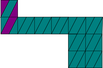
Figure 4. 2-cylinder decomposition for direction (1,2).

For direction $(-1,2)$ let $\alpha$ and $\beta$ be the waist curves of the 2-cylinder decomposition. They have strengths $3n+7$ and $1$ respectively, so that the element in $H_{1}^{(0)}(M,\mathbb{Q})$ is $X_{2}=\alpha-(3n+7)\beta$. The associated transvection is $D_{X_{2}}=Id+\iota(\cdot,\alpha)\alpha+\iota(\cdot,\beta)(3n+7)\beta$. In Figure 5 we can see the 2-cylinder decomposition for direction $(-1,2)$.

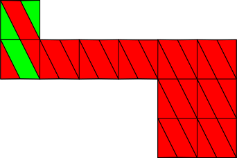
Figure 5. 2-cylinder decomposition for direction (-1,2).

Finally for the direction $(1,3)$ let $\mu$ and $\nu$ be the waist curves of the corresponding cylinder decomposition. They have strengths $2$ and $3n+4$ respectively, so that the element in $H_{1}^{(0)}(M,\mathbb{Q})$ is $X_{3}=(3n+4)\mu-2\nu$ with associated transvection is $D_{X_{3}}=Id+\iota(\cdot,\mu)(6k+1)\mu+2\iota(\cdot,\nu)2\nu$. In Figure 5 we can see the 2-cylinder decomposition for direction $(1,3)$.

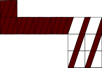
Figure 6. 2-cylinder decomposition for direction (1,3).

The data for the intersection form between the elements of the basis of $H_{1}(M,\mathbb{Q})$ and the corresponding waist curves of the directions are summarized in Table 4.

$\Omega$	$\eta$	$\lambda$	$\alpha$	$\beta$	$\mu$	$\nu$
$\sigma_{1}$	1	1	1	1	3	0
$\sigma_{2}$	1	$6n+5$	1	$6n+5$	$9n+5$	2
$\sigma_{3}$	0	4	0	4	2	2
$\xi_{1}$	-1	-1	1	1	-2	0
$\xi_{2}$	0	-1	0	1	-1	0
$\xi_{3}$	0	-3	0	3	-1	-1

Table 4. Intersections forms between the waist curves of the horizontal and vertical cylinders.

The transvections act on $e_{i}$ as follows:

$$D_{X_{1}}(e_{1})=e_{1}+(-3n-2)X_{1}\hskip 14.22636ptD_{X_{1}}(e_{2})=e_{2}-2X_{1}$$

$$D_{X_{1}}(e_{3})=e_{3}-1X_{1}\hskip 14.22636ptD_{X_{1}}(e_{4})=e_{4}$$

$$D_{X_{2}}(e_{1})=e_{1}+(-3n-2)X_{2}\hskip 14.22636ptD_{X_{2}}(e_{2})=e_{2}-2X_{2}$$

$$D_{X_{2}}(e_{3})=e_{3}+X_{2}\hskip 14.22636ptD_{X_{2}}(e_{4})=e_{4}$$

$$D_{X_{3}}(e_{1})=e_{1}-4X_{3}\hskip 14.22636ptD_{X_{3}}(e_{2})=e_{2}-4X_{3}$$

$$D_{X_{3}}(e_{3})=e_{3}\hskip 14.22636ptD_{X_{3}}(e_{4})=e_{4}+2X_{3}$$

$X_{1},X_{2},X_{3}$ are written in terms of the basis $e_{i}$ as:

$$X_{1}=-e_{1}-2e_{2}+(3n+6)e_{3}-4e_{4}$$

$$X_{2}=e_{1}+2e_{2}+(3n+6)e_{3}-4e_{4}$$

$$X_{3}=2e_{1}+(-3n-4)e_{2}+6e_{3}+(-6n-4)e_{4}$$

From this expressions we can check that steps (1) and (2) of the metacode in Section 3.2 are verified. To verify step (3) of this metacode we proceed as follows. Formula 3.1 gives the annihilator element, which is:

$$e=5X_{1}+X_{2}-(3n+6)X_{3}.$$

We choose the basis $\{X_{1},X_{3},e\}$. Since $e$ is the annihilator, $D_{X}(e)=e$. The action of the transvections on the rest of this basis is given by:

$$D_{X_{1}}(X_{3})=X_{3}-2X_{1}\hskip 14.22636pt$$

$$D_{X_{3}}(X_{1})=X_{1}+4X_{3}$$

$$D_{X_{2}}(X_{1})=(-30(n+2)+1)X_{1}+18(n+2)^{2}X_{3}-6(n+2)e$$

$$D_{X_{2}}(X_{3})=-50X_{1}+(30(n+2)+1))X_{3}-10e$$

So the transvections with respect to the basis $X_{1},X_{3},e$ are:

$$D_{X_{1}}=\begin{pmatrix}1&-2&0\\ 0&1&0\\ 0&0&1\\ \end{pmatrix},\hskip 28.45274ptD_{X_{3}}=\begin{pmatrix}1&0&0\\ 4&1&0\\ 0&0&1\\ \end{pmatrix},$$

$$D_{X_{2}}=\begin{pmatrix}-30(n+2)+1&-50&0\\ 18(n+2)^{2}&30(n+2)+1&0\\ 6(n+2)&10&1\\ \end{pmatrix}.$$

By setting $n=20k-2$, with $k\in\mathbb{N}$, the word:

$$D_{X_{3}}^{3k}D_{X_{2}}D_{X_{3}}^{-3k}D_{X_{1}}^{-25}$$

is a nontrivial element in the unipotent radical of $Sp(W)$. We conclude from that for the family $3n+8$, the subfamily $N=60k+2$ has origamis with arithmetic monodromy for $k$ large enough, that is, the proof of item (i) of Theorem 5 is complete.

3.5. Arithmeticity for the $\mathcal{F}_{3n+10}$ family

To avoid unnecessary repetitions, we condense the rest of our calculations using tables and keep the notations of the preceeding sections. In what follows we present three sets of tables. In the first set (Table 5) we present two tables, one with the information of the intersection form between an element of the base of $H_{1}(M,\mathbb{Q})$ and a waist curve for a 2-cylinder decomposition and the other with the coefficients and strengths for the respective multi-twist. The second set (Table 6) consists of only one table with six rows. The coefficients of $X_{i}$ in terms of the basis $e_{i}$ appear in the first three rows. The last three rows have the coefficients $m_{i}$ of the transvections $D_{X_{i}}(e_{i})=e_{i}+m_{i}D_{X_{i}}$. Finally (Table 7) we present the action of the transvections on a chosen basis of $W$, so that the reader can easily guess the form of the matrices, the annihilator element and a nontrivial element of the unipotent radical of $Sp(W)$. We set $n=2k-1$ so that $\theta_{1}$, $\theta_{2}$ and $\theta_{3}$ in Table 5 are vectors parallel to 2-cylinder directions.

$\Omega$	$\theta_{1}=(2,1)$		$\theta_{2}=(-2,1)$		$\theta_{3}=(1,1)$
	$\gamma_{1}$	$\gamma_{2}$	$\gamma_{1}$	$\gamma_{2}$	$\gamma_{1}$	$\gamma_{2}$
$\sigma_{1}$	0	1	0	1	1	0
$\sigma_{2}$	$3k$	$3k$	$3k$	$3k$	$6k-1$	1
$\sigma_{3}$	1	1	1	1	1	1
$\xi_{1}$	-1	-3	1	3	-2	0
$\xi_{2}$	-1	-1	1	1	-1	0
$\xi_{3}$	-4	-4	4	4	-2	-2

	$X_{1}$	$X_{2}$	$X_{3}$
$c_{1}$	1	1	1
$c_{2}$	1	1	1
$f_{1}$	$3k+4$	1	2
$f_{2}$	$3k+5$	$6k+8$	$6k+1$

Table 5. Intersections forms between the waist curves of the horizontal and vertical cylinders and data for multi-twist for the family $\mathcal{F}_{3n+10}$.

	$e_{1}$	$e_{2}$	$e_{3}$	$e_{4}$
$X_{1}$	1	3	$-(3k+3)$	1
$X_{2}$	-1	-3	$-(3k+3)$	1
$X_{3}$	4	$-(12k+2)$	4	$-6k+1$
$D_{X_{1}}$	$3k$	1	1	0
$D_{X_{2}}$	$3k$	1	-1	0
$D_{X_{3}}$	-1	-1	0	2

Table 6. Coefficients for the base in $H_{1}^{(0)}(M,\mathbb{Q})$ and coefficients for the action of the associated transvection on the elements of the base.

	$X_{1}$	$X_{3}$
$D_{X_{1}}$	$X_{1}$	$X_{3}+2X_{1}$
$D_{X_{2}}$	$(-18(k+1)+1)X_{1}+18(k+1)^{2}X_{3}-6(k+1)e$	$-18X_{1}+(18(k+1)+1))X_{3}-6e$
$D_{X_{3}}$	$X_{1}-2X_{3}$	$X_{3}$
Annihilator	$e=3X_{1}+X_{2}-3(k+1)X_{3}$
Word	$k=2l-1,D_{X_{3}}^{l}D_{X_{2}}D_{X_{3}}^{-l}D_{X_{1}}^{-9}$

Table 7. Action of each transvection on the ordered basis $X_{1},X_{3},e$ and nontrivial element $Sp(W)$.

In any event, this proves item (ii) of Theorem 5. For the remaining families we just present tables, as we have already explained how to proceed to get the results.

3.6. Arithmeticity for the $\mathcal{F}_{3n+12}$ family

We set $n=2k-1$ so that the directions give us two-cylinder decompositions.

$\Omega$	$\theta_{1}=(2,1)$		$\theta_{2}=(1,2)$		$\theta_{3}=(1,5)$
	$\gamma_{1}$	$\gamma_{2}$	$\gamma_{1}$	$\gamma_{2}$	$\gamma_{1}$	$\gamma_{2}$
$\sigma_{1}$	1	0	1	1	5	0
$\sigma_{2}$	$3k$	$3k$	$12k-1$	1	$30k-8$	2
$\sigma_{3}$	1	1	4	0	2	2
$\xi_{1}$	-3	-1	-1	-1	-2	0
$\xi_{2}$	-1	-1	-1	0	-1	0
$\xi_{3}$	-5	-5	-5	0	-1	-1

	$X_{1}$	$X_{2}$	$X_{3}$
$c_{1}$	1	1	1
$c_{2}$	1	1	4
$f_{1}$	$3k+4$	1	2
$f_{2}$	$3k+5$	$6k+8$	$6k+1$

Table 8. Intersections forms between the waist curves of the horizontal and vertical cylinders and data for multi-twist for the family $\mathcal{F}_{3n+12}$ .

	$e_{1}$	$e_{2}$	$e_{3}$	$e_{4}$
$X_{1}$	-1	-4	$3k+4$	-1
$X_{2}$	1	4	$-(6k+7)$	4
$X_{3}$	2	$-(6k+1)$	10	$-12k+2$
$D_{X_{1}}$	$-3k$	-1	-1	0
$D_{X_{2}}$	$6k-1$	2	1	0
$D_{X_{3}}$	-8	-8	0	4

Table 9. Coefficients for the base in $H_{1}^{(0)}(M,\mathbb{Q})$ and coefficients for the action of the associated transvection on the elements of the base.

	$X_{2}$	$X_{3}$
$D_{X_{1}}$	$(\dfrac{-9(k+1)}{2}+1)X_{2}+\dfrac{-3}{2}(k+1)^{2}X_{3}-3(k+1)e$	$\dfrac{27}{2}X_{2}+(\dfrac{9(k+1)}{2}+1)X_{3}-9e$
$D_{X_{2}}$	$X_{2}$	$X_{3}+6X_{2}$
$D_{X_{3}}$	$X_{2}-24X_{3}$	$X_{3}$
Annihilator	$e=X_{1}+\dfrac{3}{2}X_{2}-(\dfrac{k+1}{2})X_{3}$
Word	$k=72l-1,D_{X_{3}}^{l}D_{X_{1}}^{12}D_{X_{3}}^{-l}D_{X_{2}}^{-27}$

Table 10. Action of each transvection on the ordered basis $X_{2},X_{3},e$ and nontrivial element $Sp(W)$.

This establishes item (iii) of Theorem 5.

3.7. Arithmeticity for the $\mathcal{F}_{6n+14}$ family

The tables for this family are:

$\Omega$	$\theta_{1}=(-2,1)$		$\theta_{2}=(1,1)$		$\theta_{3}=(2,1)$
	$\gamma_{1}$	$\gamma_{2}$	$\gamma_{1}$	$\gamma_{2}$	$\gamma_{1}$	$\gamma_{2}$
$\sigma_{1}$	0	1	0	1	0	1
$\sigma_{2}$	$3n+3$	$3n+3$	1	$6n+5$	$3n+3$	$3n+3$
$\sigma_{3}$	1	1	1	1	1	1
$\xi_{1}$	1	5	0	-3	-1	-5
$\xi_{2}$	1	1	0	-1	-1	-1
$\xi_{3}$	4	4	2	-2	-4	-4

	$X_{1}$	$X_{2}$	$X_{3}$
$c_{1}$	1	1	1
$c_{2}$	1	1	1
$f_{1}$	$3n+6$	4	$3n+6$
$f_{2}$	$3n+8$	$6n+10$	$3n+8$

Table 11. Intersections forms between the waist curves of the horizontal and vertical cylinders and data for multi-twist for the family $\mathcal{F}_{6n+14}$.

	$e_{1}$	$e_{2}$	$e_{3}$	$e_{4}$
$X_{1}$	-2	-6	$-(3n+6)$	2
$X_{2}$	-4	$12n+16$	-4	$6n+6$
$X_{3}$	2	6	$-(3n+6)$	2
$D_{X_{1}}$	$3n+3$	1	-2	0
$D_{X_{2}}$	1	1	0	-2
$D_{X_{3}}$	$3n+3$	1	2	0

Table 12. Coefficients for the base in $H_{1}^{(0)}(M,\mathbb{Q})$ and coefficients for the action of the associated transvection on the elements of the base.

	$X_{2}$	$X_{3}$
$D_{X_{1}}$	$(1+36(n+2))X_{2}-36X_{3}+12e$	$36(n+2)^{2}X_{2}+(1-36(n+2))X_{3}+12(n+2)e$
$D_{X_{2}}$	$X_{2}$	$X_{3}+4X_{2}$
$D_{X_{3}}$	$X_{2}-4X_{3}$	$X_{3}$
Annihilator	$e=X_{1}-(3n+6)X_{2}+3X_{3}$
Word	$n=4k-2,D_{X_{2}}^{k}D_{X_{1}}D_{X_{2}}^{-k}D_{X_{3}}^{-9}$

Table 13. Action of each transvection on the ordered basis $X_{2},X_{3},e$ and nontrivial element $Sp(W)$.

This shows item (iv) of Theorem 5.

3.8. Arithmeticity for the $\mathcal{F}_{6n+18}$ family

Again, we do not change $n$, only later to find a subfamily and an appropriate word.

$\Omega$	$\theta_{1}=(2,1)$		$\theta_{2}=(1,1)$		$\theta_{3}=(-1,1)$
	$\gamma_{1}$	$\gamma_{2}$	$\gamma_{1}$	$\gamma_{2}$	$\gamma_{1}$	$\gamma_{2}$
$\sigma_{1}$	0	1	0	1	0	1
$\sigma_{2}$	$3n+3$	$3n+3$	1	$6n+5$	1	$6n+5$
$\sigma_{3}$	1	1	1	1	1	1
$\xi_{1}$	1	5	0	-3	0	3
$\xi_{2}$	1	1	0	-1	0	1
$\xi_{3}$	6	6	-3	-3	3	3

	$X_{1}$	$X_{2}$	$X_{3}$
$c_{1}$	1	1	1
$c_{2}$	1	1	1
$f_{1}$	$3n+8$	6	6
$f_{2}$	$3n+10$	$6n+12$	$6n+12$

Table 14. Intersections forms between the waist curves of the horizontal and vertical cylinder and data for multi-twist for the family $\mathcal{F}_{6n+18}$.

	$e_{1}$	$e_{2}$	$e_{3}$	$e_{4}$
$X_{1}$	-2	-10	$-(3n+8)$	2
$X_{2}$	-6	$18n+24$	-6	$6n+6$
$X_{3}$	6	$-(18n+24)$	-6	$6n+6$
$D_{X_{1}}$	$3n+3$	1	-2	0
$D_{X_{2}}$	1	1	0	-3
$D_{X_{3}}$	1	1	0	3

Table 15. Coefficients for the base in $H_{1}^{(0)}(M,\mathbb{Q})$ and coefficients for the action of the associated transvection on the elements of the base.

	$X_{1}$	$X_{3}$
$D_{X_{1}}$	$X_{1}$	$X_{3}+6X_{1}$
$D_{X_{2}}$	$(1+108(n+1))X_{1}-54X_{3}+18e$	$216(n+1)^{2}X_{1}+(1-108(n+1))X_{3}+36(n+1)e$
$D_{X_{3}}$	$X_{1}-6X_{3}$	$X_{3}$
Annihilator	$e=6(n+1)X_{1}+X_{2}-3X_{3}$
Word	$n=3k-1,D_{X_{1}}^{k}D_{X_{2}}D_{X_{1}}^{-k}D_{X_{3}}^{-9}$

Table 16. Action of each transvection on the ordered basis $X_{1},X_{3},e$ and nontrivial element $Sp(W)$.

This yields item (v) of Theorem 5.

3.9. Arithmeticity for the $\mathcal{F}_{6n+22}$ family

The tables of this family are:

$\Omega$	$\theta_{1}=(2,1)$		$\theta_{2}=(1,1)$		$\theta_{3}=(-1,1)$
	$\gamma_{1}$	$\gamma_{2}$	$\gamma_{1}$	$\gamma_{2}$	$\gamma_{1}$	$\gamma_{2}$
$\sigma_{1}$	0	1	0	1	0	1
$\sigma_{2}$	$3n+3$	$3n+3$	1	$6n+5$	1	$6n+5$
$\sigma_{3}$	1	1	1	1	1	1
$\xi_{1}$	1	5	0	-3	0	3
$\xi_{2}$	1	1	0	-1	0	1
$\xi_{3}$	8	8	-4	-4	4	4

	$X_{1}$	$X_{2}$	$X_{3}$
$c_{1}$	1	1	1
$c_{2}$	1	1	1
$f_{1}$	$3n+10$	8	8
$f_{2}$	$3n+12$	$6n+14$	$6n+14$

Table 17. Intersections forms between the waist curves of the horizontal and vertical cylinders and data for multi-twist for the family $\mathcal{F}_{6n+22}$.

	$e_{1}$	$e_{2}$	$e_{3}$	$e_{4}$
$X_{1}$	-2	-14	$-(3n+10)$	2
$X_{2}$	-8	$24n+32$	-8	$6n+6$
$X_{3}$	8	$-(24n+32)$	-8	$6n+6$
$D_{X_{1}}$	$3n+3$	1	-2	0
$D_{X_{2}}$	1	1	0	-4
$D_{X_{3}}$	1	1	0	4

Table 18. Coefficients for the base in $H_{1}^{(0)}(M,\mathbb{Q})$ and coefficients for the action of the associated transvection on the elements of the base.

	$X_{1}$	$X_{3}$
$D_{X_{1}}$	$X_{1}$	$X_{3}+8X_{1}$
$D_{X_{2}}$	$(1+144(n+1))X_{1}-72X_{3}-24e$	$288(n+1)^{2}X_{1}+(1-144(n+1))X_{3}-48(n+1)e$
$D_{X_{3}}$	$X_{1}-8X_{3}$	$X_{3}$
Annihilator	$e=6(n+1)X_{1}+X_{2}-3X_{3}$
Word	$n=4k-1,D_{X_{1}}^{k}D_{X_{2}}D_{X_{1}}^{-k}D_{X_{3}}^{-9}$

Table 19. Action of each transvection on the ordered basis $X_{1},X_{3},e$ and nontrivial element $Sp(W)$.

This gives the last item of Theorem 5.

4. Arithmeticity of KZ monodromies in $\mathcal{H}^{hyp}(4)$

4.1. One-parameter family of origamis in $\mathcal{H}^{hyp}(4)$

Let $\mathcal{P}_{N}$ be the origami associated to the pair of permutations:

$$h=(1)(2\dots N)\quad\textrm{and}\quad v=(1,3,2)(4,5,\dots,N).$$

Figure 7. The origami $\mathcal{P}_{N}$

Note that $\mathcal{P}_{N}\in\mathcal{H}^{hyp}(4)$ has HLK invariant $(1,[2,2,2])$ or $(0,[3,3,1])$ depending if $N$ is odd or even. Also, $\mathcal{P}_{N}$ always decomposes into three cylinders in the direction $(-1,1)$ whose waist curves $\zeta_{1}$, $\zeta_{2}$ and $\zeta_{3}$ (resp.) have holonomy vectors $(-1,1)$, $2(-1,1)$, $2(-1,1)$ (resp.) and intersect the squares labelled $1$, $2$ and $4$ (resp.). Furthermore, when $N=2n$ is even, $\mathcal{P}_{N}$ decomposes into three cylinders in the direction $(1,1)$ whose waist curves $\sigma_{1}$, $\sigma_{2}$ and $\sigma_{3}$ have holonomy vectors $(1,1)$, $(n+1)(1,1)$, $(n-1)(1,1)$.

For later use, observe that $\mathcal{P}_{N}$ decomposes into two cylinders in the directions $(1,0)$, $(0,1)$ and $(2N,1)$. In particular, the two cylinders in the direction $(1,0)$ have waist curves $\alpha_{1}$ and $\alpha_{2}$ with holonomy vectors $\textrm{hol}(\alpha_{1})=(1,0)$ and $\textrm{hol}(\alpha_{2})=(N,0)$, the two cylinders in the direction $(0,1)$ have waist curves $\beta_{1}$ and $\beta_{2}$ with holonomy vectors $\textrm{hol}(\beta_{1})=(0,3)$ and $\textrm{hol}(\beta_{2})=(0,N-2)$, and the two cylinders in the direction $(2N,1)$ have waist curves $\gamma_{1}$ and $\gamma_{2}$ with holonomy vectors $\textrm{hol}(\gamma_{1})=(2N(N-2),(N-2))$ and $\textrm{hol}(\gamma_{2})=(6N,3)$.

Thus, we can perform Dehn multi-twists with strengths $N$ for the first direction, and $3(N-2)$ for the two others to get three matrices $\widetilde{D}_{\alpha}$, $\widetilde{D}_{\beta}$ and $\widetilde{D}_{\gamma}$ in $\textrm{Sp}(H_{1}(\mathcal{P}_{N},\mathbb{Q}))$ acting on $\alpha_{i}$, $\beta_{i}$, $\gamma_{i}$, $i=1,2$, as

$$\widetilde{D}_{\alpha}(\beta_{1})=\beta_{1}+N\alpha_{1}+2\alpha_{2},\quad\widetilde{D}_{\alpha}(\beta_{2})=\beta_{2}+(N-2)\alpha_{2},$$

$$\widetilde{D}_{\alpha}(\gamma_{1})=\gamma_{1}+(N-2)\alpha_{2},\quad\widetilde{D}_{\alpha}(\gamma_{2})=\gamma_{2}+N\alpha_{1}+2\alpha_{2},$$

$$\widetilde{D}_{\beta}(\alpha_{1})=\alpha_{1}-(N-2)\beta_{1},\quad\widetilde{D}_{\beta}(\alpha_{2})=\alpha_{2}-2(N-2)\beta_{1}-3(N-2)\beta_{2},$$

$$\widetilde{D}_{\beta}(\gamma_{1})=\gamma_{1}-4(N-2)^{2}\beta_{1}-6(N-2)^{2}\beta_{2},\quad\widetilde{D}_{\beta}(\gamma_{2})=\gamma_{2}-(2N+8)(N-2)\beta_{1}-12(N-2)\beta_{2},$$

and

$$\widetilde{D}_{\gamma}(\alpha_{1})=\alpha_{1}-(N-2)\gamma_{2},\quad\widetilde{D}_{\gamma}(\alpha_{2})=\alpha_{2}-3(N-2)\gamma_{1}-2(N-2)\gamma_{2},$$

$$\widetilde{D}_{\gamma}(\beta_{1})=\beta_{1}+12(N-2)\gamma_{1}+(N-2)(2N+8)\gamma_{2},\quad\widetilde{D}_{\gamma}(\beta_{2})=\beta_{2}+6(N-2)^{2}\gamma_{1}+4(N-2)^{2}\gamma_{2}$$

Hence, the restrictions $D_{\alpha}$, $D_{\beta}$ and $D_{\gamma}$ of these matrices to $H_{1}^{(0)}(\mathcal{P}_{N},\mathbb{Q})$ act on $\alpha=\alpha_{2}-N\alpha_{1}$, $\beta=3\beta_{2}-(N-2)\beta_{1}$ and $\gamma=3\gamma_{1}-(N-2)\gamma_{2}$ as

$$D_{\alpha}(\beta)=\beta+(N-2)\alpha,\quad D_{\alpha}(\gamma)=\gamma+(N-2)\alpha$$

$$\quad D_{\beta}(\alpha)=\alpha-(N-2)\beta,\quad D_{\beta}(\gamma)=\gamma-2(N-2)^{2}\beta$$

and

$$D_{\gamma}(\alpha)=\alpha-(N-2)\gamma,\quad D_{\gamma}(\beta)=\beta+2(N-2)^{2}\gamma.$$

4.1.1. Zariski denseness of the KZ monodromy of $\mathcal{P}_{2n}$

By inspecting the intersections between the cycles $\sigma_{i}$ and $\zeta_{j}$ for $i,j\in\{1,2,3\}$, we see that the matrices $\widetilde{A}$ and $\widetilde{B}$ of the Dehn multi-twists in the directions $(1,1)$ and $(-1,1)$ with strengths $(n-1)(n+1)$ and $2$ in the basis $\{\sigma_{1},\sigma_{2},\sigma_{3},\zeta_{1},\zeta_{2},\zeta_{3}\}$ are $\widetilde{A}(\sigma_{i})=\sigma_{i}$, $\widetilde{B}(\zeta_{i})=\zeta_{i}$ for $1\leq i\leq 3$, and

$$\widetilde{A}(\zeta_{1})=\zeta_{1}+(n-1)\sigma_{2}+(n+1)\sigma_{3},\quad\widetilde{A}(\zeta_{2})=\zeta_{2}+(n^{2}-1)\sigma_{1}+3(n-1)\sigma_{2},$$

$$\widetilde{A}(\zeta_{3})=\zeta_{3}+(n^{2}-1)\sigma_{1}+2(n-1)\sigma_{2}+(n+1)\sigma_{3},\quad\widetilde{B}(\sigma_{1})=\sigma_{1}+\zeta_{2}+\zeta_{3},$$

$$\widetilde{B}(\sigma_{2})=\sigma_{2}+2\zeta_{1}+3\zeta_{2}+2\zeta_{3},\quad\widetilde{B}(\sigma_{3})=\sigma_{3}+2\zeta_{1}+\zeta_{3}.$$

Thus, the matrices $A$ and $B$ of the restrictions of these actions to $H_{1}^{(0)}(\mathcal{P}_{2n},\mathbb{Q})$ with respect to the basis $\Sigma_{2,1}=\sigma_{2}-(n+1)\sigma_{1}$, $\Sigma_{3,1}=\sigma_{3}-(n-1)\sigma_{1}$, $Z_{2,1}=\zeta_{2}-2\zeta_{1}$, $Z_{3,1}=\zeta_{3}-2\zeta_{1}$ are

$$A=\left(\begin{array}[]{cccc}1&0&n-1&0\\ 0&1&-2(n+1)&-(n+1)\\ 0&0&1&0\\ 0&0&0&1\end{array}\right),\quad B=\left(\begin{array}[]{cccc}1&0&0&0\\ 0&1&0&0\\ -n+2&-n+1&1&0\\ -n+1&-n+2&0&1\end{array}\right).$$

The characteristic polynomial of $AB$ is $x^{4}+ax^{3}+bx^{2}+ax+1$ with $a=-2(n^{2}+n-1)$ and $b=2n^{3}+n^{2}+2n-3$. Hence, $t=-a-4$ and $d=b+2a+2$ are positive for all $n$ sufficiently large, and

$$\Delta_{1}=4(n^{4}-2n^{2}-4n+6),\quad\Delta_{2}=(2n^{3}+5n^{2}+6n-5)(2n-3)(n+1)(n-1),$$

so that $AB$ is Galois-pinching for all $n$ sufficiently large. Since $\mathcal{P}_{2n}$ decomposes into two cylinders in many directions, it follows that the KZ monodromy of $\mathcal{P}_{2n}$ is Zariski dense in $\textrm{Sp}(H_{1}^{(0)}(\mathcal{P}_{2n},\mathbb{Q}))$ for all $n$ sufficiently large.

4.1.2. Arithmeticity of the KZ monodromy of $\mathcal{P}_{2n}$

We are ready to study the actions of $D_{\alpha}$, $D_{\beta}$ and $D_{\gamma}$ on the three-dimensional subspace $W$ of $H_{1}^{(0)}(\mathcal{P}_{N},\mathbb{R})$ spanned by $\alpha$, $\beta$ and $\gamma$. The vector

$$e=2(N-2)\alpha+\beta-\gamma\in W$$

satisfies $\Omega(e,w)=0$ for all $w\in W$. Finally, the matrices of the restrictions of $D_{\alpha}$, $D_{\beta}$ and $D_{\gamma}$ to $W$ with respect to the basis $\{\alpha,\beta,e\}$ are

$$D_{\alpha}|_{W}=\left(\begin{array}[]{ccc}1&N-2&0\\ 0&1&0\\ 0&0&1\end{array}\right),\,D_{\beta}|_{W}=\left(\begin{array}[]{ccc}1&0&0\\ -N+2&1&0\\ 0&0&1\end{array}\right)$$

and

$$D_{\gamma}|_{W}=\left(\begin{array}[]{ccc}1-2(N-2)^{2}&4(N-2)^{3}&0\\ -N+2&1+2(N-2)^{2}&0\\ N-2&-2(N-2)^{2}&1\end{array}\right)$$

In particular,

$$(D_{\alpha}|_{W})^{-2}(D_{\gamma}|_{W})(D_{\alpha}|_{W})^{2}(D_{\beta}|_{W})^{-1}=\left(\begin{array}[]{ccc}1&0&0\\ 0&1&0\\ N-2&0&1\end{array}\right)$$

is a non-trivial element of the unipotent radical of $\textrm{Sp}_{\Omega}(W)$.

In summary, we showed the following statement:

Theorem 9.

The KZ monodromy / shadow Veech group of $\mathcal{P}_{2n}$ is arithmetic for all but finitely many choices of $n\in\mathbb{N}$.

5. Arithmeticity of certain Stairs Origamis in genus $4$

Let $N\geq 4$ and $M:=4+2m$ with $m\geq 0$ We now consider $\mathcal{O}_{N,M}$, the Origami associated to the pair of permutations $h,v\in\mbox{Sym}(\{1,\dots,N+M+2\})$, where

$$h= (1,2,3\dots,N)(N+1,N+2,N+3)(N+4,N+5)(N+6)\dots(M)$$

$$v= (1,\ N+1,\ N+4,\ N+6,\dots,N+M)(2,\ N+2,\ N+5)(3,\ N+3)(4)\dots(N).$$

Figure 8. Origami $\mathcal{O}_{N,M}$ with horizontal waist curves $\sigma_{1},\sigma_{2},\sigma_{3},\sigma_{N}$ and vertical waist curves $\zeta_{1},\zeta_{2},\zeta_{3},\zeta_{M}$.

5.1. Our favourite Dehn twists

In this subsection we use cylinder decompositions of the Origami $\mathcal{O}_{N,M}$ in several directions to construct Dehn twists on it. These twists act on the homology $H_{1}(\mathcal{O}_{N,M},\mathbb{Q})$ and preserve the intersection form $\Omega$. With this procedure we can find elements in $\mbox{Sp}_{\Omega}(H_{1}^{(0)}(\mathcal{O}_{N,M},\mathbb{Q}))$, which will be the cornerstone of the arguments in this section.

The waist curves $\sigma_{1},\sigma_{2},\sigma_{3},\sigma_{N}$ of the four maximal vertical cylinders and the four waist curves $\zeta_{1},\zeta_{2},\zeta_{3},\zeta_{M}$ of the four maximal horizontal cylinders form a basis of $H_{1}(\mathcal{O}_{N,M},\mathbb{Z})$ (see figure 8). We have the follwing holonomy vectors for these waist curves:

$$\begin{array}[]{cccc}\mbox{hol}(\sigma_{1})=(1,0),&\mbox{hol}(\sigma_{2})=(2,0),&\mbox{hol}(\sigma_{3})=(3,0),&\mbox{hol}(\sigma_{N})=(N,0)\\ \mbox{hol}(\zeta_{1})=(0,1),&\mbox{hol}(\zeta_{2})=(0,2),&\mbox{hol}(\zeta_{3})=(0,3),&\mbox{hol}(\zeta_{M})=(0,M).\end{array}$$

We have that $B^{(0)}:=\{\Sigma_{1},\Sigma_{2},\Sigma_{N},Z_{1},Z_{2},Z_{M}\}$ is a basis of the non-tautological part $H^{(0)}(\mathcal{O}_{N,M},\mathbb{Z})$, where

$$\begin{array}[]{ccc}\Sigma_{1}=\sigma_{2}-2\sigma_{1},&\Sigma_{2}=\sigma_{3}-3\sigma_{1},&\Sigma_{N}=\sigma_{N}-N\sigma_{1},\\ Z_{1}=\zeta_{2}-2\zeta_{1},&Z_{2}=\zeta_{3}-3\zeta_{2};&Z_{M}=\zeta_{M}-M\zeta_{1}.\end{array}$$

The symplectic intersection-form $\Omega$ has the following representation-matrix on $H^{(0)}(\mathcal{O}_{N,M},\mathbb{Z})$ with respect to the basis $B^{(0)}$ from above:

$$\left(\begin{array}[]{cccccc}0&0&0&0&1&-1\\ 0&0&0&1&1&-2\\ 0&0&0&-1&-2&-N-M+1\\ 0&-1&1&0&0&0\\ -1&-1&2&0&0&0\\ 1&2&N+M-1&0&0&0\end{array}\right)$$

With cylinder decompositions of $\mathcal{O}_{N,M}$ in directions $(1,1)$, $(1,-1)$, $(1,2)$, $(1,-2)$ as well as the horizontal and vertical direction we can construct Dehn-twists along the waist curves of the cylinders. These twists induce actions on $H_{1}^{(0)}(\mathcal{O}_{N,M},\mathbb{Z}))$, which we want to present in the following.

Figure 9. Origami $\mathcal{O}_{N,M}$ with cylinder decomposition in direction $(1,1)$.

Figure 10. Origami $\mathcal{O}_{N,M}$ with cylinder decomposition in direction $(1,-1)$.

For the direction $(1,1)$ we have a decomposition into two maximal cylinders with waist curves $\delta_{1}$ of length $3$ and $\delta_{2}$ of length $N+M-1$ (see figure 10). In direction $(1,-1)$ we also have a decomposition into two maximal cylinders (see figure 10). We denote the waist curve of length $5$ by $\chi_{1}$ and the waist curve of length $N+M-3$ by $\delta_{2}$. The associated Dehn twists along the waist curves of these maximal cylinders act as transvections $D_{\delta}$ and $D_{\chi}$ on $H_{1}^{(0)}(\mathcal{O}_{N,M},\mathbb{Z})$ via the following mapping rules:

$$D_{\delta}\colon v\longmapsto v+(N+M-1)\ \Omega(\delta_{1},v)\delta_{1}+3\ \Omega(\delta_{2},v)\delta_{2}$$

$$D_{\chi}\colon v\longmapsto v+(N+M-3)\ \Omega(\chi_{1},v)\chi_{1}+5\ \Omega(\chi_{2},v)\chi_{2}$$

As in the previous sections we count intersection points of the curves $\sigma_{i},\sigma_{N},\zeta_{i},\zeta_{M}$ $(i=1,2,3)$ with the waist curves of the cylinders:

$$\begin{array}[]{llll}\Omega(\delta_{1},\sigma_{1})=0,&\Omega(\delta_{2},\sigma_{1})=-1,&\Omega(\delta_{1},\zeta_{1})=0,&\Omega(\delta_{2},\zeta_{1})=1\\ \Omega(\delta_{1},\sigma_{2})=-1,&\Omega(\delta_{2},\sigma_{2})=-1,&\Omega(\delta_{1},\zeta_{2})=1,&\Omega(\delta_{2},\zeta_{2})=1\\ \Omega(\delta_{1},\sigma_{3})=-1,&\Omega(\delta_{2},\sigma_{3})=-2,&\Omega(\delta_{1},\zeta_{3})=1,&\Omega(\delta_{2},\zeta_{3})=2\\ \Omega(\delta_{1},\sigma_{N})=-1,&\Omega(\delta_{2},\sigma_{N})=-(N-1),&\Omega(\delta_{1},\zeta_{M})=1,&\Omega(\delta_{2},\zeta_{M})=M-1\end{array}$$

For the cylinder in direction $(1,-1)$ with waist curves $\chi_{1},\chi_{2}$ we get:

$$\begin{array}[]{llll}\Omega(\chi_{1},\sigma_{1})=0,&\Omega(\chi_{2},\sigma_{1})=1,&\Omega(\chi_{1},\zeta_{1})=0,&\Omega(\chi_{2},\zeta_{1})=1\\ \Omega(\chi_{1},\sigma_{2})=1,&\Omega(\chi_{2},\sigma_{2})=1,&\Omega(\chi_{1},\zeta_{2})=1,&\Omega(\chi_{2},\zeta_{2})=1\\ \Omega(\chi_{1},\sigma_{3})=2,&\Omega(\chi_{2},\sigma_{3})=1,&\Omega(\chi_{1},\zeta_{3})=2,&\Omega(\chi_{2},\zeta_{3})=1\\ \Omega(\chi_{1},\sigma_{N})=2,&\Omega(\chi_{2},\sigma_{N})=N-2,&\Omega(\chi_{1},\zeta_{M})=2,&\Omega(\chi_{2},\zeta_{M})=M-2\end{array}$$

These intersection points allow us to determine representation-matrices $M_{\delta}^{(0)}$ and $M_{\chi}^{(0)}$ for the transvections $D_{\delta},D_{\chi}\in\mbox{Sp}_{\Omega}(H_{1}^{(0)}(\mathcal{O}_{N,M},\mathbb{Z}))$ with respect to $B^{(0)}$:

$$\begin{array}[]{rl}M_{\delta}^{(0)}=&\footnotesize\left(\begin{array}[]{cccccc}4&3&3&-3&-3&-3\\ -N-M+1&-N-M+2&-N-M+1&N+M-1&N+M-1&N+M-1\\ 3&3&4&-3&-3&-3\\ 3&3&3&-2&-3&-3\\ -N-M+1&-N-M+1&-N-M+1&N+M-1&N+M&N+M-1\\ 3&3&3&-3&-3&-2\end{array}\right),\\ &\\ M_{\chi}^{(0)}=&\footnotesize\left(\begin{array}[]{cccccc}M+N-2&2M+2N-6&2M+2N-6&M+N-3&2M+2N-6&2M+2N-6\\ M+N-3&2M+2N-5&2M+2N-6&M+N-3&2M+2N-6&2M+2N-6\\ -5&-10&-9&-5&-10&-10\\ -M-N+3&-2M-2N+6&-2M-2N+6&-M-N+4&-2M-2N+6&-2M-2N+6\\ -M-N+3&-2M-2N+6&-2M-2N+6&-M-N+3&-2M-2N+7&-2M-2N+6\\ 5&10&10&5&10&11\end{array}\right).\end{array}$$

Figure 11. Origami $\mathcal{O}_{N,M}$ with cylinder decomposition in direction $(1,2)$.

Figure 12. Origami $\mathcal{O}_{N,M}$ with cylinder decomposition in direction $(1,-2)$.

For the directions $(1,2)$ and $(1,-2)$ we have again decompositions into two cylinders (see figure 12 and figure 12). For direction $(1,2)$ the waist curves $\gamma_{1}$, $\gamma_{2}$ have length $M$ and $2N+M+4$. For direction $(1,-2)$ the waist curves $\alpha_{1}$, $\alpha_{2}$ have length $N+m$ and $m+6$. We get the following transvections $D_{\gamma}$ and $D_{\alpha}$:

$$D_{\gamma}\colon v\longmapsto v+(2N+M+4)\ \Omega(\gamma_{1},v)\gamma_{1}+M\ \Omega(\gamma_{2},v)\gamma_{2}$$

$$D_{\alpha}\colon v\longmapsto v+(m+6)\ \Omega(\alpha_{1},v)\alpha_{1}+(N+m)\ \Omega(\alpha_{2},v)\alpha_{2}$$

For the intersection points of the waist curve $\gamma_{1},\gamma_{2}$ and $\alpha_{1},\alpha_{2}$ with $\sigma_{i},\sigma_{N},\zeta_{i},\zeta_{M}$ we counted

$$\begin{array}[]{llll}\Omega(\gamma_{1},\sigma_{1})=-1,&\Omega(\gamma_{2},\sigma_{1})=-1,&\Omega(\gamma_{1},\zeta_{1})=0,&\Omega(\gamma_{2},\zeta_{1})=1,\\ \Omega(\gamma_{1},\sigma_{2})=-1,&\Omega(\gamma_{2},\sigma_{2})=-3,&\Omega(\gamma_{1},\zeta_{2})=0,&\Omega(\gamma_{2},\zeta_{2})=2,\\ \Omega(\gamma_{1},\sigma_{3})=-1,&\Omega(\gamma_{2},\sigma_{3})=-5,&\Omega(\gamma_{1},\zeta_{3})=1,&\Omega(\gamma_{2},\zeta_{3})=2,\\ \Omega(\gamma_{1},\sigma_{N})=-1,&\Omega(\gamma_{2},\sigma_{N})=1-2N,&\Omega(\gamma_{1},\zeta_{M})=1+m,&\Omega(\gamma_{2},\zeta_{M})=3+m,\end{array}$$

respectively

$$\begin{array}[]{llll}\Omega(\alpha_{1},\sigma_{1})=1,&\Omega(\alpha_{2},\sigma_{1})=1,&\Omega(\alpha_{1},\zeta_{1})=1,&\Omega(\alpha_{2},\zeta_{1})=0,\\ \Omega(\alpha_{1},\sigma_{2})=1,&\Omega(\alpha_{2},\sigma_{2})=3,&\Omega(\alpha_{1},\zeta_{2})=1,&\Omega(\alpha_{2},\zeta_{2})=1,\\ \Omega(\alpha_{1},\sigma_{3})=2,&\Omega(\alpha_{2},\sigma_{3})=4,&\Omega(\alpha_{1},\zeta_{3})=1,&\Omega(\alpha_{2},\zeta_{3})=2,\\ \Omega(\alpha_{1},\sigma_{N})=2N-4,&\Omega(\alpha_{2},\sigma_{N})=4,&\Omega(\alpha_{1},\zeta_{M})=1+m,&\Omega(\alpha_{2},\zeta_{M})=3+m.\\ \end{array}$$

With this data we calculated that the maps $D_{\gamma},D_{\alpha}$ have the follwing representation matrices $M_{\gamma}^{(0)}$ and $M_{\alpha}^{(0)}$ on $H_{1}^{(0)}(\mathcal{O}_{N,M},\mathbb{Z})$ :

$$\begin{array}[]{rl}M_{\gamma}^{(0)}=&\footnotesize\left(\begin{array}[]{cccccc}M+2N+5&2M+4N+8&(N-1)(M+2N+4)&0&M+2N+4&(m+1)(M+2N+4)\\ -M&-2M+1&-(N-1)M&0&-M&-(m+1)M\\ -M&-2M&-(N-1)M+1&0&-M&-(m+1)M\\ -2M&-4M&-2(N-1)M&1&-2M&-2(m+1)M\\ -2M&-4M&-2(N-1)M&0&-2M+1&-2(m+1)M\\ 2N+4&4N+8&(N-1)(2N+4)&0&2N+4&(m+1)(2N+4)+1\end{array}\right),\\ &\\ M_{\alpha}^{(0)}=&\footnotesize\left(\begin{array}[]{cccccc}N+m+1&N+m&-(N-4)(N+m)&N+m&2(N+m)&(3+m)(N+m)\\ N+m&N+m+1&-(N-4)(N+m)&N+m&2(N+m)&(3+m)(N+m)\\ -m-6&-m-6&(N-4)(m+6)+1&-m-6&-2(m+6)&-(3+m)(m+6)\\ -N+6&-N+6&(N-4)(N-6)&-N+7&2(-N+6)&-(3+m)(N-6)\\ -2(N+m)&-2(N+m)&2(N-4)(N+m)&-2(N+m)&-4(N+m)+1&-2(3+m)(N+m)\\ -N+6&-N+6&(N-4)(N-6)&-N+6&2(-N+6)&-(3+m)(N-6)+1\end{array}\right).\\ \end{array}$$

Figure 13. Origami $\mathcal{O}_{N,M}$ with cylinder decomposition in direction $(1,0)$.

Figure 14. Origami $\mathcal{O}_{N,M}$ with cylinder decomposition in direction $(0,1)$.

For a cylinder $C=\mathbb{R}/k\mathbb{Z}\times(0,a)$ we call the fraction $m=k/a$ the modulus of $C$. In the cylinder decomposition of the origami $\mathcal{O}_{N,M}$ in horizontal, respectively vertical direction we have in both cases four maximal cylinders with moduli $1/(M-3),\ 2/1,\ 3/1,\ N/1$ for the horizontal direction and moduli $1/(N-3),\ 2/1,\ 3/1,\ M/1$ for the vertical direction (see figure 14 and figure 14). So we get two twists which act on $H_{1}^{(0)}(\mathcal{O}_{N,M},\mathbb{Z})$ by the following mapping rules:

$$D_{h}\colon w\mapsto w+6(M-3)N\ \Omega(\sigma_{1},w)\sigma_{1}+3N\ \Omega(\sigma_{2},w)\sigma_{2}+2N\ \Omega(\sigma_{3},w)\sigma_{3}+6\ \Omega(\sigma_{N},w)\sigma_{N},$$

$$D_{v}\colon w\mapsto w+6(N-3)M\ \Omega(\zeta_{1},w)\zeta_{1}+3M\ \Omega(\zeta_{2},w)\zeta_{2}+2M\ \Omega(\zeta_{3},w)\zeta_{3}+6\ \Omega(\zeta_{M},w)\zeta_{M}.$$

It is now easy to calculate representation matrices $M_{h}^{(0)}$ and $M_{v}^{(0)}$ for the action of the horizontal and vertical twist on $H_{1}^{(0)}(\mathcal{O}_{N,M},\mathbb{Z})$ with respect to $B^{(0)}$:

$$\begin{array}[]{rl}M_{h}^{(0)}=&\left(\begin{array}[]{cccccc}1&0&0&0&3N&3N\\ 0&1&0&2N&2N&2N\\ 0&0&1&-6&-12&-6(M-1)\\ 0&0&0&1&0&0\\ 0&0&0&0&1&0\\ 0&0&0&0&0&1\end{array}\right),\\ M_{v}^{(0)}=&\left(\begin{array}[]{cccccc}1&0&0&0&0&0\\ 0&1&0&0&0&0\\ 0&0&1&0&0&0\\ 0&-3M&-3M&1&0&0\\ -2M&-2M&-2M&0&1&0\\ 6&12&6(N-1)&0&0&1\end{array}\right).\end{array}$$

5.2. Zariski density in genus $4$

For the proof of the Zariski-density of $\mbox{Sp}_{\Omega}(H_{1}^{(0)}(\mathcal{O}_{N,M},\mathbb{C}))$ in the case of the Origami $\mathcal{O}_{N,M}$, we will first follow an idea which differs from the original one in the previous sections. Let us describe theidea first before we go into the details:

We choose first a $\mathbb{Z}$-submodule $\Gamma_{N,M}$ of $H_{1}^{(0)}(\mathcal{O}_{N,M},\mathbb{Z})$ such that we can identify these elements of $\mbox{Sp}_{\Omega}(H_{1}^{(0)}(\mathcal{O}_{N,M},\mathbb{Z}))$, which stabilize $\Gamma_{N,M}$ with elements of the standard symplectic group $\mbox{Sp}_{6}(\mathbb{Z})$. The key ingredient of our arguments is the following Proposition of Detinko, Flannery and Hulpke.

Theorem 10 (Detinko, Flannery, Hulpke, [10] Prop. 3.7).

Suppose that a subgroup $H\leq\text{Sp}_{2n}(\mathbb{Z})$ contains a transvection $t\in H$. Then $H$ is Zariski dense if and only if the normal closure $\langle t\rangle^{H}$ of $t$ in $H$ is absolutely irreducible.

Therefore our goal is to find a transvection $t$ in the image $G$ of the action

$$\mbox{Aff}^{+}(\mathcal{O}_{N,M})\longrightarrow\mbox{Sp}_{\Omega}(H_{1}^{(0)}(\mathcal{O}_{N,M},\mathbb{Z})),$$

which stabilizes the lattice $\Gamma_{N,M}$ and to show that the normal closure $\langle t\rangle^{H}$ is absolutely irreducible, where we identify $H:=G\cap\mbox{Stab}_{\Gamma_{N,M}}(\mbox{Sp}_{\Omega}(H_{1}^{(0)}(\mathcal{O}_{N,M},\mathbb{Z})))$ with a subgroup of $\text{Sp}_{6}(\mathbb{Z})$. We will see that this procedure leads to the Zariski-density of $\mbox{Sp}_{\Omega}(H_{1}^{(0)}(\mathcal{O}_{N,M},\mathbb{Z}))$ only for finitely many $N,M\in\mathbb{N}$ since we used the computer to proof the irreducibility of $\langle t\rangle^{H}$.

Nevertheless it seems to be possible to find infinitely many $N,M\in\mathbb{N}$ such that $\mbox{Sp}_{\Omega}(H_{1}^{(0)}(\mathcal{O}_{N,M},\mathbb{Z}))$ is Zariski-dense, if we again use Galois-theoretical arguments (see Remark 11).

We now start going into details. Consider the $\mathbb{Z}$-submodule $\Gamma_{N,M}$ of $H_{1}^{(0)}(\mathcal{O}_{N,M},\mathbb{Z})$ generated by the following elements:

$$\begin{array}[]{ll}c_{1}:=(N+M+2)\Sigma_{1},&c_{2}:=(N+M+2)(-2\Sigma_{1}-\ \Sigma_{N}),\\ c_{3}:=(-1-N-M)Z_{1}+Z_{2}+Z_{M}&c_{4}:=Z_{2},\\ c_{5}:=Z_{1},&c_{6}:=\Sigma_{1}+\Sigma_{2}+\Sigma_{N}\end{array}$$

The submodule $\Gamma_{N,M}$ has finite index in $H_{1}^{(0)}(\mathcal{O}_{N,M},\mathbb{Z})$ and if we restrict the symplectic intersection-form $\Omega$ to $\Gamma_{N,M}$ we get the following matrix-representation $I_{C}^{\Omega}\in\mathbb{R}^{6\times 6}$ with respect to the basis $C:=\{c_{1},c_{2},c_{3},c_{4},c_{5},c_{6}\}$:

$$I_{C}^{\Omega}:=\left(\begin{array}[]{cccccc}0&0&0&N+M+2&0&0\\ 0&0&0&0&N+M+2&0\\ 0&0&0&0&0&N+M+2\\ -N-M-2&0&0&0&0&0\\ 0&-N-M-2&0&0&0&0\\ 0&0&-N-M-2&0&0&0\end{array}\right)$$

Let $G$ be the image of the action $\mbox{Aff}^{+}(\mathcal{O}_{N,M})\to\mbox{Sp}_{\Omega}(H_{1}^{(0)}(\mathcal{O}_{N,M},\mathbb{Z}))$. We conclude that the elements $\phi\in G$, which stabilize the lattice $\Gamma_{N,M}$, can be identified with elements of the standard symplectic group $\mbox{Sp}_{6}(\mathbb{Z})$, i.e

$$H:=G\cap\mbox{Stab}_{\Gamma}(\mbox{Sp}_{\Omega}(H_{1}^{(0)}(\mathcal{O}_{N,M},\mathbb{Z})))\leq\mbox{Sp}_{6}(\mathbb{Z}).$$

We want to describe the elements of $\mbox{Sp}_{\Omega}(H_{1}^{(0)}(\mathcal{O}_{N,M},\mathbb{Z}))$, which stabilize the lattice $\Gamma_{N,M}$. Respectively we want to find conditions for their matrix-representations to do so. Denote by $C\in\mathbb{R}^{6\times 6}$ the matrix, which has as columns the coefficients of the vectors $c_{i}$ $(i=1,\dots,6)$ written as a linear combination of elements in $B^{(0)}$. Furthermore let $C^{-1}\in\mathbb{Q}^{6\times 6}$ be the inverse of $C$, i.e

$$\begin{array}[]{rl}C=&\left(\begin{array}[]{cccccc}N+M+2&1&-2(N+M+2)&0&0&0\\ 0&1&0&0&0&0\\ 0&1&-(N+M+2)&0&0&0\\ 0&0&0&1&0&-1-N-M\\ 0&0&0&0&1&1\\ 0&0&0&0&0&1\end{array}\right),\\ &\\ C^{-1}=&\left(\begin{array}[]{cccccc}\frac{1}{N+M+2}&\frac{1}{N+M+2}&\frac{-2}{N+M+2}&0&0&0\\ 0&1&0&0&0&0\\ 0&\frac{1}{N+M+2}&\frac{-1}{N+M+2}&0&0&0\\ 0&0&0&1&0&N+M+1\\ 0&0&0&0&1&-1\\ 0&0&0&0&0&1\end{array}\right).\end{array}$$

An element $\phi\in\mbox{Sp}_{\Omega}(H_{1}^{(0)}(\mathcal{O}_{N,M},\mathbb{Z}))$ stabilizes the lattice $\Gamma_{N,M}$ if and only if $\phi(c_{i})$ is an element of $\mbox{Span}_{\mathbb{Z}}(\{c_{1},\dots,c_{6}\})$ for each $i\in\{1,\dots,6\}$ or equivalent

$$C^{-1}\cdot D_{B^{(0)}}(\phi(c_{i})))\in\mathbb{Z}^{6}$$

for every $i\in\{1,\dots,6\}$, here we write $D_{B^{(0)}}(\phi(c_{i}))\in\mathbb{R}^{6}$ for the coefficients of $\phi(c_{i})$, written as a linear-combination of elements in the basis $B^{(0)}$.

Thus $\phi$ stabilizes $\Gamma_{N,M}$ if and only if for each $i\in\{1,\dots,6\}$ the element $D_{B^{(0)}}(\phi(c_{i}))$ is in both the kernels of the following two maps

$$g_{1}\colon\mathbb{Z}^{6}\longrightarrow\mathbb{Z}{/}(N+M+2)\mathbb{Z}, \quad(v_{1},\dots v_{6})\longmapsto\overline{v_{1}+v_{2}-2v_{3}}$$

$$g_{2}\colon\mathbb{Z}^{6}\longrightarrow\mathbb{Z}{/}(N+M+2)\mathbb{Z}, \quad(v_{1},\dots v_{6})\longmapsto\overline{v_{2}-v_{3}}.$$

Easy but boring calculations show that for every $i\in\{1,\dots,6\}$ and every matrix $M$ in the set $\{M_{\delta}^{(0)},\ M_{\chi}^{(0)},\ M_{\gamma}^{(0)},\ M_{\alpha}^{(0)},\ M_{v}^{(0)}\}$, we have

$$M\cdot D_{B^{(0)}}(c_{i})\in\mbox{ker}(g_{1})\cap\mbox{ker}(g_{2}).$$

Hence $D_{\delta},D_{\chi},D_{\gamma},D_{\alpha},D_{v}\in\mbox{Stab}_{\Gamma_{N,M}}(\mbox{Sp}_{\Omega}(H_{1}^{(0)}(\mathcal{O}_{N,M},\mathbb{Z})))$. Furthermore $(M_{h}^{(0)}-I_{6})^{2}=\underline{0}$ and so we conclude with the Bernoulli-formula $(M_{h}^{(0)})^{N+M+2}\equiv I_{6}\ (\mbox{mod}\ N+M+2)$. Hence

$$(M_{h}^{(0)})^{N+M+2}\cdot D_{B^{(0)}}(c_{i})\in\mbox{ker}(g_{1})\cap\mbox{ker}(g_{2})$$

Consider the algebra $A_{N,M}$ generated by the transvection $t:=M_{\delta}^{(0)}$ and the elements $M^{-1}tM\in\langle t\rangle^{H}$ where

$$M\in\{M_{\chi}^{(0)},M_{\gamma}^{(0)},M_{\alpha}^{(0)},M_{v}^{(0)},(M_{h}^{(0)})^{N+M+2}\}.$$

Here $\langle t\rangle^{H}$ denotes the normal closure of the transvection $t$ in $H$. For $N\in\{4,5,...,50\}$ and $m\in\{0,1,...,50\}$ we calculated with GAP $\mbox{dim}_{\mathbb{Q}}(A_{N,M})=36$ for the vector space dimension of the algebra $A_{N,M}$. This shows that $\langle t\rangle^{H}$ is an absolutely irreducible group and for these cases we conclude with Theorem 10 that $H$ is Zariski dense in $\mbox{Sp}_{\Omega}(H_{1}^{(0)}(\mathcal{O}_{N,M},\mathbb{C}))$.

Remark 11.

Even though we have not fully investigated this direction, it seems possible to obtain the Zariski denseness of $H$ for infinitely many choices of the parameters $N$ and $M$ by developing the Galois-theoretical method in Subsection 2.2. In fact, since $B=M_{\delta}^{(0)}$ doesn’t commute with $A=M_{h}^{(0)}\cdot M_{v}^{(0)}$, the task is to check that $A$ is Galois-pinching (for many choices of $N$ and $M$). For this sake, one can note that the characteristic polynomial of $A$ is a reciprocal, sextic polynomial $P$ such that $\frac{1}{x^{3}}P(x)=Q(x+\frac{1}{x}+2)$ for a cubic polynomial $Q$. Since the discriminants of $Q$ and $P$ are positive for many choices of $N$ and $M$, we have that $Q$ has three real distinct roots $\mu_{1}$, $\mu_{2}$, $\mu_{3}$, and $P$ has six distinct roots. Given that the coefficients of $Q$ are positive (for many choices of $N$ and $M$), $\mu_{1},\mu_{2},\mu_{3}<0$ and, a fortiori, $P$ has the six real (negative) roots $\lambda_{1}$, $\lambda_{1}^{-1}$, $\lambda_{2}$, $\lambda_{2}^{-1}$, $\lambda_{3}$, $\lambda_{3}^{-1}$ with $\mu_{\ell}=\lambda_{\ell}+\lambda_{\ell}^{-1}$ and $|\lambda_{\ell}|>1$ for $\ell=1,2,3$. Furthermore, $Q$ is irreducible modulo $5$ when $N\equiv 1\equiv M$ modulo $5$, and $P$ is irreducible modulo $19$ when $N\equiv 1\equiv M$ modulo $19$, so that $Q$ and $P$ are irreducible over $\mathbb{Q}$ when $N\equiv 1\equiv M$ modulo $95$. In particular, $Q$ has Galois group $S_{3}$ when its discriminant is not a square, and Siegel’s theorem can be used to verify that this is the case for $N=96$ and all but finitely many choices of $M$. Hence, the Galois group $Gal$ of $P$ is a transitive subgroup of the hyperoctahedral group $\mathcal{G}=\mathbb{Z}_{2}^{3}\rtimes S_{3}$ whose projection on the $S_{3}$-factor is surjective. It is known that $\mathcal{G}$ has three maximal subgroups containing $\{(+1,+1,+1)\}\times S_{3}$, namely, $N_{1}=\{(\varepsilon_{1},\varepsilon_{2},\varepsilon_{3},\sigma):\varepsilon_{1}\varepsilon_{2}\varepsilon_{3}=1\}$, $N_{2}=\{(\varepsilon_{1},\varepsilon_{2},\varepsilon_{3},\sigma):\varepsilon_{1}\varepsilon_{2}\varepsilon_{3}\cdot\textrm{sign}(\sigma)=1\}$, and $K=\{(+1,+1,+1),(-1,-1,-1)\}\times S_{3}$. Thus, we could ensure that $Gal=\mathcal{G}$ (and $A$ is Galois-pinching) using that Siegel’s theorem to say that some appropriate discriminants are not squares or non-trivial powers (for $N=96$ and infinitely many choices of $M$, say).

5.3. Arithmeticity in genus $4$

For each of the cylinder decompositions in direction $(1,1)$, $(1,-1)$ and $(1,2)$ we get two maximal cylinders. We denote their waist curves by $\delta_{1},\delta_{2}\in H_{1}(\mathcal{O}_{N,M},\mathbb{Z})$ for direction $(1,1)$, by $\chi_{1},\chi_{2}\in H_{1}(\mathcal{O}_{N,M},\mathbb{Z})$ for the waist curves of cylinders in direction $(1,-1)$ and by $\gamma_{1},\gamma_{2}$ for the waist curves in direction $(1,2)\in H_{1}(\mathcal{O}_{N,M},\mathbb{Z})$. If we compare the length of these waist curves we can see that the following elements have zero holonomy, respectively are elements of the non-tautological part $H_{1}^{(0)}(\mathcal{O}_{N,M},\mathbb{Z})$:

$$\Delta: =(N+M-1)\delta_{1}-3\delta_{2}$$

$$=-3\Sigma_{1}+(N+M-1)\Sigma_{2}-3\Sigma_{N}-3Z_{1}+(N+M-1)Z_{2}-3Z_{M},$$

$$X: =(N+M-3)\chi_{1}-5\chi_{2}$$

$$=(N+M-3)\Sigma_{1}+(N+M-3)\Sigma_{2}-5\Sigma_{N}-(N+M-3)Z_{1}-(N+M-3)Z_{2}-5Z_{M},$$

$$\Gamma: =(2N+M+4)\gamma_{1}-M\gamma_{2}$$

$$=(2N+M+4)\Sigma_{1}-M\Sigma_{2}-M\Sigma_{N}-2MZ_{1}-2MZ_{2}+(2N+4)Z_{M}.$$

Set $W:=\mbox{Span}_{\mathbb{Q}}(\Delta,\ X,\ \Gamma)$. The vector space $W$ has dimension $\mbox{dim}_{\mathbb{Q}}(W)=3$. We set $A:=22-4N-4M$, $B:=6+3m$ and $C:=12-3N+9m$. Restricted to $W$ the transvections $D_{\delta},\ D_{\chi}$ and $D_{\gamma}$ have the following matrix representations with respect to the basis $\{\Delta,\ X,\ \Gamma\}$:

$$\left(\begin{array}[]{ccc}1&A&-2B\\ 0&1&0\\ 0&0&1\end{array}\right),\quad\left(\begin{array}[]{ccc}1&0&0\\ -A&1&-2C\\ 0&0&1\end{array}\right),\quad\left(\begin{array}[]{ccc}1&0&0\\ 0&1&0\\ B&C&1\end{array}\right)$$

The vector $e:=-2C\Delta+2BX+A\Gamma$ is fixed by all the three elements $D_{\delta},\ D_{\chi}$ and $D_{\gamma}$ and with respect to the new basis $\{\Delta,\ X,\ e\}$ we get the following matrix representations for them:

$$\left(\begin{array}[]{ccc}1&A&0\\ 0&1&0\\ 0&0&1\end{array}\right),\quad\left(\begin{array}[]{ccc}1&0&0\\ -A&1&0\\ 0&0&1\end{array}\right),\quad\left(\begin{array}[]{ccc}2\frac{BC}{A}+1&2\frac{C^{2}}{A}&0\\ -2\frac{B^{2}}{A}&-2\frac{BC}{A}+1&0\\ \frac{B}{A}&\frac{C}{A}&1\end{array}\right)$$

Now if we choose $C=0$ or equivalent $N=3m+4$, then the group generated by $D_{\delta}|_{W},~{}D_{\chi}|_{W},~{}D_{\gamma}|_{W}$ contains a non-trivial element of the unipotent radical of the symplectic group on $W$, namely $(D_{\chi}|_{W})^{-2B^{2}}\circ(D_{\gamma}|_{W})^{A^{2}}$ is represented by

$$\begin{pmatrix}1&0&0\\ 0&1&0\\ BA&0&1\end{pmatrix}$$

with respect to the basis $\{\Delta,\ X,\ e\}$. This ends the proof of Theorem 2.

6. Computational results

In this section we consider origamis $\mathcal{O}$ of genus $g$ without translations and denote by $M$ the corresponding translation surface. Recall that in this case the affine group of $\mathcal{O}$ is identified with the Veech group $\Gamma(\mathcal{O})$ and hence acts on the homology $H_{1}(M,\mathbb{Z})$. Its action can be computed explicitly (see [22, Section 3]). From this one obtains the shadow Veech group as restriction to the non-tautological part $H_{1}^{(0)}(M,\mathbb{Z})$. Choosing a suitable basis and a suitable sublattice in $H_{1}^{(0)}(M,\mathbb{Z})$ we can compute finite index subgroups of the shadow Veech groups which lie in $\operatorname{Sp}(2g-2,\mathbb{Z})$. This is implemented in [11] and was used by the authors for computer experiments whose results are presented in this section. We use that $\operatorname{SL}(2,\mathbb{Z})$ is generated by the two matrices $S$ and $T$ with

$$S=\begin{pmatrix}0&-1\\ 1&0\end{pmatrix}\mbox{ and }T=\begin{pmatrix}1&1\\ 0&1\end{pmatrix}$$

6.1. Origamis in genus 2

In genus 2 it is known by a result of Möller (cf. Appendix B) that the shadow Veech groups of origamis are arithmetic. In this case the shadow Veech groups are subgroups of $\operatorname{SL}(2,\mathbb{Z})=\operatorname{Sp}(2,\mathbb{Z})$. We systematically compute the shadow Veech groups of origamis in genus 2 of small degree by computer-assisted computations and detect a nice pattern from these computer experiments.

6.1.1. The stratum $\mathcal{H}(2)$

Recall that the $\operatorname{SL}(2,\mathbb{Z})$-orbits of origamis of degree $n$ in $\mathcal{H}(2)$ are classified by Hubert/Lelièvre and McMullen (cf. [21],[31]) in the following way: For each $n$ there are at most 2 orbits. More precisely, if $n$ is even or 3, then there is only one orbit. If $n$ is odd an not 3, then there are 2 orbits called $A_{n}$ and $B_{n}$ distinguished by their number of integer Weierstrass points. The origamis in the orbit $A_{n}$ have 1 integer Weierstrass point whereas the origamis in the orbit $B_{n}$ have 3 integer Weierstrass points.

Computations in GAP with the package [11] give the following results in $\mathcal{H}(2)$: Let $n$ be the number of squares of the origami $(M,\omega)$. For $n\leq 21$ we obtain:

• If $n$ is even, then $[\operatorname{SL}_{2}(\mathbb{Z}):\operatorname{SL}^{(0)}(M,\omega)]=3$.

• If $n$ is odd and $O$ lies in the orbit $A_{n}$, then $[\operatorname{SL}_{2}(\mathbb{Z}):\operatorname{SL}^{(0)}(M,\omega)]=1$

• If $n$ is odd and $O$ lies in the orbit $B_{n}$, then $[\operatorname{SL}_{2}(\mathbb{Z}):\operatorname{SL}^{(0)}(M,\omega)]=3$

From the classification of the orbits it follows in particular that each orbit can be represented by an $L$-shaped origami $L(a,b)$. The degree is then $n=a+b-1$. And for $n$ odd $L(a,b)$ lies in the orbit $A_{n}$, if $a$ and $b$ are even, it lies in $B_{n}$, if $a$ and $b$ are odd. The shadow Veech groups of origamis in the same orbit are conjugated. Hence in order to obtain the result above it suffices to study for each $n$ one respectively two $L$-shaped origami of degree $n$ depending on $n$ being even or odd.

6.1.2. The stratum $\mathcal{H}(1,1)$

In the following we consider origamis $O=O(k,l)$ of degree $n=k+l$ given by the following permutations:

$$\sigma_{h}=(1,2,\ldots,k)(k+1,\ldots,n),\quad\sigma_{v}=(k,k+1)$$

We obtain – again by computations with [11] – the following pattern for the index of the shadow Veech group in $\operatorname{SL}(2,\mathbb{Z})$. Observe that if and only if $k=l$, then the translation surface allows a translation. Hence we have to exclude those surfaces from the computations since we only consider surfaces without translations.

$$\begin{array}[]{c|cccccccccccccccccccc}l\backslash k&2&3&4&5&6&7&8&9&10&11&12&13&14&15&16&17&18&19&20&21\\ \hline\cr 2&-&1&1&1&6&1&1&1&3&1&1&1&6&1&1&1&3&1&1&1\\ 3&1&-&1&3&4&3&1&3&1&3&1&3&1&12&1&3&1&3&1&3\\ 4&1&1&-&1&1&1&1&1&1&1&6&1&1&1&1&1&1&1&3&1\\ 5&1&3&1&-&1&3&1&3&1&3&1&3&1&3&1&3&1&3&12&3\\ 6&6&4&1&1&-&1&1&1&6&1&4&1&3&1&1&1&6&1&1&4\\ 7&1&3&1&3&1&-&1&3&1&3&1&3&1&3&1&3&1&3&1&3\\ 8&1&1&1&1&1&1&-&1&1&1&1&1&1&1&1&1&1&1&1&1\\ 9&1&3&1&3&1&3&1&-&1&3&1&3&1&3&1&3&4&3&1&3\\ 10&3&1&1&1&6&1&1&1&-&1&1&1&6&12&1&1&3&1&1&1\\ 11&1&3&1&3&1&3&1&3&1&-&1&3&1&3&1&3&1&3&1&3\\ 12&1&1&6&1&4&1&1&1&1&1&-&1&1&4&1&1&1&1&24&1\\ 13&1&3&1&3&1&3&1&3&1&3&1&-&1&3&1&3&1&3&1&3\\ 14&6&1&1&1&3&1&1&1&6&1&1&1&-&1&1&1&6&1&1&1\\ 15&1&12&1&3&1&3&1&3&12&3&4&3&1&-&1&3&1&3&1&12\\ 16&1&1&1&1&1&1&1&1&1&1&1&1&1&1&-&1&1&1&1&1\\ 17&1&3&1&3&1&3&1&3&1&3&1&3&1&3&1&-&1&3&1&3\\ 18&3&1&1&1&6&1&1&4&3&1&1&1&6&1&1&1&-&1&1&1\\ 19&1&3&1&3&1&3&1&3&1&3&1&3&1&3&1&3&1&-&1&3\\ 20&1&1&3&12&1&1&1&1&1&1&24&1&1&1&1&1&1&1&-&1\\ 21&1&3&1&3&4&3&1&3&1&3&1&3&1&12&1&3&1&3&1&-\end{array}$$

6.2. An example in genus 3

We study in this section the shadow Veech group of the origami $\mathcal{O}=\mathcal{O}_{3,5}=((1,2,3,4,5)(6,7),(1,6,8)(2,7))\in\mathcal{H}^{odd}(4)$ (see Figure 15) which is the smallest member of the family of origamis studied in Section 3.3. Consider the basis $B=\{\sigma_{l},\sigma_{m},\sigma_{c},\zeta_{l},\zeta_{m},\zeta_{c}\}$ of $H_{1}(\mathcal{O},\mathbb{Z})$ (see Figure 15) and the basis $C=\{\Sigma_{l}=\sigma_{l}-5\sigma_{c},\Sigma_{m}=\sigma_{m}-2\sigma_{c},Z_{l}=\zeta_{l}-3\zeta_{c},Z_{m}=\zeta_{m}-2\zeta_{c}\}$ of $H_{1}^{(0)}(\mathcal{O},\mathbb{Z})$ defined at the beginning of Section 3.3.

Figure 15. The origami $\mathcal{O}=\mathcal{O}_{3,5}$

Computing the Veech group $\Gamma(\mathcal{O})$ with the programs from [11], we obtain that it is an index 1020 subgroup of $\operatorname{SL}(2,\mathbb{Z})$ with 102 generators. Let $\rho^{sh}_{C}:\Gamma(\mathcal{O})\to\operatorname{SL}(4,\mathbb{Z})$ be the action of the Veech group on the non tautological part $H_{1}^{(0)}(\mathcal{O},\mathbb{Z})$, where $H_{1}^{(0)}(\mathcal{O},\mathbb{Z})$ is identified with $\mathbb{Z}^{4}$ according to the chosen basis $C$. We want to study the image $H=\rho^{sh}_{C}(\Gamma(\mathcal{O}))\subseteq\operatorname{SL}(4,\mathbb{Z})$, i.e. the group of all matrices obtained from the transformations in the shadow Veech group with respect to the basis $C$ of $H_{1}^{(0)}(\mathcal{O},\mathbb{Z})$. From Section 3.3 we know that it is an arithmetic group. Recall that the action of the shadow Veech group respects the intersection form, but that there is no symplectic basis of $H_{1}^{(0)}(\mathcal{O},\mathbb{Z})$ defined over $\mathbb{Z}$ . Hence $H$ can not be conjugated to a subgroup of $\operatorname{Sp}(4,\mathbb{Z})$. But we may pass to a finite index subgroup of $H$ which is conjugated to a subgroup $\tilde{H}$ of $\operatorname{Sp}(4,\mathbb{Z})$ of finite index (see below). Now, recall that $\operatorname{Sp}(4,\mathbb{Z})$ has the congruence subgroup property, i.e. any finite index subgroup of $\operatorname{Sp}(4,\mathbb{Z})$ is a congruence groups of some level $l$. We determine with GAP and in particular with the package [10] the index and the level $l$ of the group $\tilde{H}\subseteq\operatorname{Sp}(4,\mathbb{Z})$ .
In detail, this is achieved for this example as follows. Observe that the intersection form on the homology restricted to $H_{1}^{(0)}(\mathcal{O},\mathbb{Z})$ has the fundamental matrix $G$ given in (6.1) with respect to the basis $C$.

$$G=\begin{pmatrix}0&0&7&1\\ 0&0&1&-1\\ -7&-1&0&0\\ -1&1&0&0\\ \end{pmatrix},\quad T=\begin{pmatrix}1&1&0&0\\ 0&1&0&0\\ 0&0&0&1\\ 0&0&1&-7\\ \end{pmatrix},\quad G^{\prime}=T^{t}GT=\begin{pmatrix}0&0&1&0\\ 0&0&0&8\\ -1&0&0&0\\ 0&-8&0&0\\ \end{pmatrix}$$ (6.1)

The determinant of $G$ is 64. Hence we cannot find a symplectic basis of $H_{1}^{(0)}(\mathcal{O},\mathbb{Z})$ defined over $\mathbb{Z}$. However, we do the base change given by the transformation matrix $T$ from (6.1) such that the fundamental matrix of the intersection form with respect to this new basis $C^{\prime}=(c^{\prime}_{1},c^{\prime}_{2},c^{\prime}_{3},c^{\prime}_{4})$ becomes the matrix $G^{\prime}$ in (6.1). Define $\Lambda$ to be the lattice generated by $\tilde{C}=(8c^{\prime}_{1},c^{\prime}_{2},c^{\prime}_{3},c^{\prime}_{4})$. Then the intersection form on $\Lambda$ has the fundamental matrix $\tilde{G}$ in (6.2).

$$\tilde{G}=\begin{pmatrix}0&0&8&0\\ 0&0&0&8\\ -8&0&0&0\\ 0&-8&0&0\\ \end{pmatrix},\quad\tilde{T}=\begin{pmatrix}8&0&0&0\\ 0&1&0&0\\ 0&0&1&0\\ 0&0&0&1\end{pmatrix}$$ (6.2)

Observe that a matrix $A$ in $\operatorname{SL}(4,\mathbb{Z})$ lies in $\operatorname{Sp}(4,\mathbb{Z})$ if and only if the corresponding linear transformation respects $\tilde{G}$, i.e. if and only if $A^{t}\cdot\tilde{G}\cdot A=\tilde{G}$. We now have to restrict to those elements in $H^{\prime}:=T^{-1}HT$ which stabilise the lattice $\Lambda$, i.e. we consider

$$\textrm{Stab}_{H^{\prime}}(\Lambda)=\{A\in H^{\prime}|\;\forall x\in\Lambda:A\cdot x\in\Lambda\}.$$

Computing $\textrm{Stab}_{H^{\prime}}(\Lambda)$ with [25] we obtain that it is a subgroup of index 48 in $H^{\prime}$. Now we do the base change described by the transformation matrix $\tilde{T}$ in (6.2)in order to express the elements of $H^{\prime}$ with respect to the basis $\tilde{C}$. In this way we obtain $\tilde{H}=\tilde{T}\cdot H^{\prime}\cdot\tilde{T}^{-1}$ as a subgroup of $\operatorname{Sp}(4,\mathbb{Z})$. From computations in GAP in particular using [10] we obtain that $\tilde{H}$ is a congruence subgroup of level 16 and of index 46080 in $\operatorname{Sp}(4,\mathbb{Z})$.

6.3. A non dense shadow Veech group in genus 4

In this subsection we consider the origami $\mathcal{O}=((2,3,4)(5,7,6),(1,2,3,5,4,6,7))$ of degree 7 and genus 4 in stratum $\mathcal{H}(6)$, see Figure 16.

Figure 16. Origami $\mathcal{O}$ in $\mathcal{H}(6)$: edges with same labels and unlabelled opposite edges are glued

Its Veech group $\Gamma(O)$ is a subgroup of index 8 in $\operatorname{SL}(2,\mathbb{Z})$ generated by the two parabolic matrices

$$A_{1}=\begin{pmatrix}1&3\\ 0&1\end{pmatrix}\mbox{ and }A_{2}=\begin{pmatrix}1&0\\ -1&1\end{pmatrix}.$$

The coset graph is shown in Figure 17 on the left side. Observe that $\Gamma(\mathcal{O})$ does not contain the matrix $-I$. Hence its image $\mathbb{P}\Gamma(\mathcal{O})$ in $\mathbb{P}\operatorname{SL}(2,\mathbb{Z})$ is a subgroup of index 4. Its coset graph is shown in Figure 17 on the right side. $\mathbb{P}\Gamma(\mathcal{O})$ has two cusps of width 3 and width 1, respectively. They correspond two the $\overline{T}$-orbits where $\overline{T}$ is the image of $T$ in $\mathbb{P}\operatorname{SL}(2,\mathbb{Z})$.

Figure 17. The coset graph of $\Gamma(O)$ in $\operatorname{SL}(2,\mathbb{Z})$ (left side) and of $\mathbb{P}\Gamma(O)$ in $\mathbb{P}\operatorname{SL}(2,\mathbb{Z})$ (right side). The dashed arrows show the action of $S$, the non-dashed arrows the action of $T$.

We denote in the following by $e_{i}$ the lower edge of the square in $\mathcal{O}$ labelled with $i$ and with $e_{i+7}$ the left edge of the square labelled with $i$. Then $B=\{e_{1},e_{3},e_{4},e_{5},e_{7},e_{8},e_{9},e_{13}\}$ forms a basis of $H_{1}(M,\mathbb{Z})$. The two generators $A_{1}$ and $A_{2}$ of the Veech group $\Gamma(\mathcal{O})$ act on $H_{1}(M,\mathbb{Z})$ with respect to this basis by the two matrices:

$$B_{1}=\begin{pmatrix}1&0&0&0&0&3&1&1\\ 0&1&0&0&0&0&1&0\\ 0&0&1&0&0&0&1&1\\ 0&0&0&1&0&0&0&0\\ 0&0&0&0&1&0&0&1\\ 0&0&0&0&0&1&0&0\\ 0&0&0&0&0&0&1&0\\ 0&0&0&0&0&0&0&1\end{pmatrix},\quad B_{2}=\begin{pmatrix}1&1&1&1&1&-1&-1&0\\ 0&0&0&0&0&1&0&0\\ 0&1&1&1&0&0&-1&0\\ 0&0&-1&-1&0&0&1&0\\ 0&-1&0&0&0&0&1&0\\ 0&0&0&0&-1&0&0&1\\ -1&0&0&-1&0&1&0&0\\ 0&-1&-1&0&0&0&1&0\end{pmatrix}$$

The non tautological part $H_{1}^{(0)}(M,\mathbb{Z})$ of the homology has the following basis:

$$C:=\{v_{1}=e_{1}-e_{7},\;v_{2}=e_{3}-e_{7},\;v_{3}=e_{4}-e_{7},\;v_{4}=e_{5}-e_{7},\;v_{5}=e_{8}-e_{13},\;v_{6}=e_{9}-e_{13}\}$$

The action of $A_{1}$ and $A_{2}$ on $H_{1}^{(0)}(M,\mathbb{Z})$ with respect to $C$ is then given by the following two matrices:

$$C_{1}=\begin{pmatrix}1&0&0&0&2&0\\ 0&1&0&0&0&1\\ 0&0&1&0&-1&0\\ 0&0&0&1&0&0\\ 0&0&0&0&1&0\\ 0&0&0&0&0&1\end{pmatrix},\quad C_{2}=\begin{pmatrix}0&0&0&0&-1&-1\\ 0&0&0&0&1&0\\ 0&1&1&1&0&-1\\ 0&0&-1&-1&0&1\\ 1&1&1&1&-1&-1\\ -1&0&0&-1&1&0\end{pmatrix}$$

Hence for this example the shadow Veech group is isomorphic to the subgroup of $\operatorname{SL}(6,\mathbb{Z})$ generated by $C_{1}$ and $C_{2}$. A computation with GAP gives us that the $\mathbb{Q}$-algebra $\mathbb{Q}(C_{1},C_{2})$ generated by $C_{1}$ and $C_{2}$ has dimension 18 and thus not the full dimension. We conclude that the shadow Veech group is not dense in this case.

Appendix A Example of KZ monodromy in the Prym locus of $\mathcal{H}^{odd}(4)$

Recall that an origami $(M,\omega)$ in the Prym locus of $\mathcal{H}^{odd}(4)$ has KZ monodromy included in $\textrm{Sp}(H_{1}^{+})\times\textrm{Sp}(H_{1}^{-})\simeq SL(2,\mathbb{Z})\times SL(2,\mathbb{Z})$ because the affine homeomorphisms of $(M,\omega)$ respect the splitting $H_{1}^{(0)}(M,\mathbb{Q})=H_{1}^{+}\oplus H_{1}^{-}$ associated to the eigenspaces (of the eigenvalues $\pm 1$) of the anti-automorphism of $(M,\omega)$ (see, e.g., [27]). In particular, the KZ monodromy of an origami in the Prym locus of $\mathcal{H}^{odd}(4)$ is not Zariski dense in $\textrm{Sp}(H_{1}^{(0)}(M,\mathbb{R}))\simeq\textrm{Sp}(4,\mathbb{R})$, but we can still ask about the arithmeticity of KZ monodromies in this context. The answer to this question is not clear in general.

For example, let us consider the case of the origami $\mathcal{E}_{5}$ associated to the permutations $h=(1,2)(3)(4,5)$ and $v=(1)(2,4,3)(5)$ to disclose the kind of question one finds by studying this locus.

Figure 18. The Origami in the Prym locus

By using SageMath, one has that the Veech group of $\mathcal{E}_{5}$ is an index 10 subgroup of $SL(2,\mathbb{Z})$ generated by the matrices

$$\left(\begin{array}[]{cc}1&2\\ 0&1\end{array}\right),\left(\begin{array}[]{cc}5&-2\\ 3&-1\end{array}\right),\left(\begin{array}[]{cc}-4&3\\ -7&5\end{array}\right).$$

Since

$$\left(\begin{array}[]{cc}5&-2\\ 3&-1\end{array}\right)=\left(\begin{array}[]{cc}1&2\\ 0&1\end{array}\right)\left(\begin{array}[]{cc}-1&0\\ 3&-1\end{array}\right)\quad\textrm{and}\quad\left(\begin{array}[]{cc}5&-2\\ 3&-1\end{array}\right)\left(\begin{array}[]{cc}-4&3\\ -7&5\end{array}\right)=\left(\begin{array}[]{cc}-6&5\\ -5&4\end{array}\right)$$

the Veech group of $\mathcal{E}_{5}$ is also generated by

$$\left(\begin{array}[]{cc}1&2\\ 0&1\end{array}\right),\left(\begin{array}[]{cc}1&0\\ 3&1\end{array}\right),\left(\begin{array}[]{cc}-1&0\\ 0&-1\end{array}\right),\left(\begin{array}[]{cc}6&-5\\ 5&-4\end{array}\right).$$

Observe that $\mathcal{E}_{5}$ has three horizontal cylinders with waist curves $\sigma_{1}$, $\sigma_{0}$, $\sigma_{2}$ with holonomies $(2,0)$, $(1,0)$, $(2,0)$, and three vertical cylinders with waist curves $\zeta_{1}$, $\zeta_{0}$, $\zeta_{2}$ with holonomies $(0,1)$, $(0,3)$, $(0,1)$, so that $H_{1}^{(0)}(\mathcal{E}_{5},\mathbb{Q})$ has a basis consisting of $\Sigma_{i}=\sigma_{i}-2\sigma_{0}$, $Z_{i}=3\zeta_{i}-\zeta_{0}$, $i=1,2$. Moreover, $-\textrm{Id}_{2\times 2}$ acts on $H_{1}^{(0)}(\mathcal{E}_{5},\mathbb{Q})$ by $\Sigma_{i}\mapsto-\Sigma_{3-i}$, $Z_{i}\mapsto-Z_{3-i}$, $i=1,2$, so that

$$H_{1}^{(0)}(\mathcal{E}_{5},\mathbb{Q})=H_{1}^{+}\oplus H_{1}^{-}$$

where $H_{1}^{+}$ is generated by $\Sigma^{+}=\Sigma_{1}-\Sigma_{2}$, $Z^{+}=Z_{1}-Z_{2}$, and $H_{1}^{-}$ is spanned by $\Sigma^{-}=\Sigma_{1}+\Sigma_{2}$ and $Z^{-}=Z_{1}+Z_{2}$. A direct computation reveals that the matrices $A$ and $B$ of the actions of $\left(\begin{array}[]{cc}1&2\\ 0&1\end{array}\right)$ and $\left(\begin{array}[]{cc}1&0\\ 3&1\end{array}\right)$ on the basis $\{\Sigma^{+},Z^{+},\Sigma^{-},Z^{-}\}$ of $H_{1}^{+}\oplus H_{1}^{-}$ are

$$A=\left(\begin{array}[]{cccc}1&3&0&0\\ 0&1&0&0\\ 0&0&1&1\\ 0&0&0&1\end{array}\right)\quad\textrm{and}\quad B=\left(\begin{array}[]{cccc}1&0&0&0\\ 1&1&0&0\\ 0&0&1&0\\ 0&0&1&1\end{array}\right).$$

Moreover, the matrix $\left(\begin{array}[]{cc}6&-5\\ 5&-4\end{array}\right)$ acts trivially on $H_{1}^{(0)}(M,\mathbb{Q})$ because it induces a Dehn multitwist in the one-cylinder direction $(1,1)$.

The action of $A$ and $B$ restricted to $H_{1}^{-}$ generate a copy of $SL(2,\mathbb{Z})$ since the matrices

$$T=\left(\begin{array}[]{cc}1&1\\ 0&1\end{array}\right),S=\left(\begin{array}[]{cc}1&0\\ 1&1\end{array}\right)$$

are generators. Similarly, $A$ and $B$ restricted to $H_{1}^{+}$ generate a group $\Gamma$ which is a copy of the finite-index subgroup $\Gamma_{1}(3)$ of $SL(2,\mathbb{Z})$.

However, we have not further investigated how the group spanned by $A$ and $B$ sits inside the product $\Gamma\times SL(2,\mathbb{Z})$.

Appendix B Shadow Veech groups for genus two Origamis

The goal of this section is to prove Theorem 23 (an unpublished result of Martin Möller), stating that the shadow Veech group, respectively the Kontsevich-Zorich monodromy of an origami in genus $g=2$ has finite index in $\mbox{SL}_{2}(\mathbb{Z})$.

B.1. Preliminaries

B.1.1. Local systems

The next Theorem is very important for the study of the representations in our context. For a proof see for example [40] section 3.1.1.

Theorem 12.

Let $R$ be a ring and let $X$ be a path-connected, locally simply connected topological space with a base point $x\in X$. Then there is an equivalence between the category of $R$-local systems on $X$ and the category of $R$-modules with $\pi_{1}(X,x)$-left action, given by the functor

$$\mathbb{L}\longmapsto\mathbb{L}_{x},$$

where $\mathbb{L}_{x}$ denotes the stalk of the $R$-local system $\mathbb{L}$ at the base point $x\in X$.

The mapping on $\mathbb{L}_{x}$, induced by the left action of $\pi_{1}(X,x)$, is called monodromy representation.

B.1.2. Translation structures

Let $X$ be a compact Riemann surface of genus $g$ with finitely many marked points $\Sigma\subset X$. A translation structure on $X{\setminus}\Sigma$ is determined by an atlas $(V,\phi)$ with an open covering $V=(V_{i})_{i\in I}$ of $X{\setminus}\Sigma$ and with charts $\phi_{i}\colon V_{i}\to\mathbb{C}$ such that the transition maps $\phi_{i,j}\colon\mathbb{C}\to\mathbb{C}$ are of the form

$$\phi_{i,j}(z_{i})=z_{j}+c_{i,j}$$

on the intersection $V_{i}\cap V_{j}$.

Denote by $\Omega T_{g}$ the bundle over the Teichmüller space $T_{g}$ whose points parametrize pairs $(X,\omega)$ of a compact, marked Riemann surface $X$ together with a non-zero holomorphic 1-form $\omega$.

For a point $(X,\omega)\in\Omega T_{g}$, let $Z(\omega)\subset X$ be the set of zeros of $\omega$. We can define a translation chart on $X{\setminus}Z(\omega)$ in the following way: Choose a point $x\in X{\setminus}Z(\omega)$, now for every simply connected $U\subset X{\setminus}Z(\omega)$ define a map

$$\phi_{U}\colon U\longrightarrow\mathbb{C},\quad y\longmapsto\int_{x}^{y}\omega.$$

Then $(U,\phi_{U})$ is one of the translation charts.

On the other hand given a compact Riemann surface $X$ of genus $g$ with a finite set of points $\Sigma\subset X$ and a translation atlas $(V,\phi_{i})$ for $X{\setminus}\Sigma$, we can pull back the holomorphic 1-form $dz$ on $\mathbb{C}$ via the charts $(V_{i},\phi_{i})$ to get a holomorphic 1-form $\omega{{}^{\prime}}$ on $X{\setminus}\Sigma$. It is now easy to extend $\omega{{}^{\prime}}$ to a holomorphic 1-form $\omega$ on $X$.

The following proposition is standard and plausible considering the last arguments:

Proposition 13.

On compact Riemann surfaces, flat structures are in one-to-one correspondence with holomorphic 1-forms.

B.1.3. Teichmüller curves

We first want to give the definition and construction of Teichmüller curves in the sense of [32] section 1.3. As additional literature we can recommend [28] as well as [30] section 2 and 3 and for a more intense approach have a look in [33] section 2 and 3.

Let $S$ be a compact Riemann surface of genus $g$ and $\Sigma\subset S$ a set of $n\geq 0$ marked points. We denote by $T_{g}(S,\Sigma)$ the Teichmüller space of compact Riemann surfaces $X$ of genus $g\geq 1$ with markings $m\colon S\to X$. We write $\Gamma_{g}(S,\Sigma)$ for the mapping class group of $T_{g}(S,\Sigma)$ and $M_{g}(S,\Sigma)$ for the moduli space of compact Riemann surfaces of genus $g$. In most of the cases we are not interested in the base point $(S,\text{id})$ of $T_{g}(S,\Sigma)$ and write $T_{g}$ for $T_{g}(S,\Sigma)$ respectively $\Gamma_{g}$ and $M_{g}$ for $\Gamma_{g}(S,\Sigma)$ and $M_{g}(S,\Sigma)$.

We will now explain how to construct Teichmüller curves from certain points $(X,\omega)\in\Omega T_{g}$. We can define an $\mbox{SL}_{2}(\mathbb{R})$-action on $\Omega T_{g}$ in the following way: Given $A={\tiny\begin{pmatrix}a&b\\ c&d\end{pmatrix}}\in\mbox{SL}_{2}(\mathbb{R})$ and $(X,\omega)\in\Omega T_{g}$ consider the harmonic 1-form

$$\omega_{A}=\begin{pmatrix}1&i\end{pmatrix}\begin{pmatrix}a&b\\ c&d\end{pmatrix}\begin{pmatrix}\mbox{Re}(\omega)\\ \mbox{Im}(\omega)\end{pmatrix}$$

on $X$. We can equip $X$ with a new complex structure, with respect to which $\omega_{A}$ is holomorphic. This complex structure delivers a new Riemann surface $X_{A}$ and we define $A.(X,\omega):=(X_{A},\omega_{A})\in\Omega T_{g}$.

The fibers of the projection $\Omega T_{g}\to T_{g}$ are stabilized by $\mbox{SO}_{2}(\mathbb{R})$ and for $(X,\omega)\in\Omega T_{g}$ the projection of the orbit $\Delta:=\mbox{SL}_{2}(\mathbb{R}).(X,\omega)\subset\Omega T_{g}$ to $T_{g}$ is an embedding. Thus we get for every translation surface $(X,\omega)\in\Omega T_{g}$ a map

$$\iota\colon\mathbb{H}=\mbox{SL}_{2}(\mathbb{R}){/}\mbox{SO}_{2}(\mathbb{R})\longrightarrow T_{g},$$

which is a geodesic embedding for the Teichmüller metric on $T_{g}$ (see [32] section 1.2).

By composing $\iota$ with the projection map $\pi_{g}\colon T_{g}\to M_{g}$, we get a map

$$f\colon\mathbb{H}=\mbox{SL}_{2}(\mathbb{R}){/}\mbox{SO}_{2}(\mathbb{R})\longrightarrow M_{g}.$$

The global stabilizer of the action of $\Gamma_{g}$ on $\Delta:=\iota(\mathbb{H})\subset T_{g}$ is the group $\mbox{Aff}^{+}(X,\omega)$ of orientation preserving diffeomorphisms, which are affine with respect to the translation structure defined by $\omega$. We denote the stabilizer

$$\mbox{Stab}(f)=\{A\in\mbox{Aut}(\mathbb{H})\mid f(At)=f(t)\ \forall t\in\mathbb{H}\}$$

by $\mbox{SL}(X,\omega)$ and we want to point out that $R\cdot\mbox{SL}(X,\omega)\cdot R$ coincides with the Veech group of $(X,\omega)$, where $R=\text{diag}(1,-1)$ ([30] Prop. 3.2) Since $\iota$ is injective, we have an isomorphism $\mathbb{H}{/}\mbox{SL}(X,\omega)\cong\Delta{/}\mbox{Aff}^{+}(X,\omega)$. We now call

$$j\colon\mathbb{H}{/}\mbox{SL}(X,\omega)\to M_{g}$$

or $C_{1}:=\Delta{/}\mbox{Aff}^{+}(X,\omega)$ a Teichmüller curve if one of the following equivalent statements is true:

1. The stabilizer group $\mbox{SL}(X,\omega)\subset\mbox{Aut}(\mathbb{H})$ is a lattice.

2. The manifold $\Delta{/}\mbox{Aff}^{+}(X,\omega)$ has finite volume or equivalent has finitely many cusps and no big holes, respectively flaring ends.

In this case the map $j\colon C_{1}\to M_{g}$ is proper and generically injective. Its image $j(C_{1})\subset M_{g}$ is an algebraic curve, whose normalization is $C_{1}$ (see [30] section 2). If the curve $C_{1}$ was constructed from a pair $(X,\omega)\in\Omega T_{g}$, we say that $(X,\omega)$ generates the Teichmüller curve $C_{1}$. The construction made above is visualized in the following diagram:

Remark 14.

If $(X,\omega)=\mathcal{O}$ defines an origami, the group $\mbox{SL}(X,\omega)$ is a finite index subgroup of $\mbox{SL}_{2}(\mathbb{Z})$ (see [20]). This implies that $\mbox{SL}(X,\omega)$ is a lattice in $\mbox{Aut}(\mathbb{H})$ and hence every origami defines a Teichmüller curve. We will call a Teichmüller curve, which comes from an origami, a origami-curve.

B.1.4. Family of curves

We recall the construction of the family of curves coming from a Teichmüller curve as in section 1.4 in [32] or section 3.1 in [33].

Let $j\colon C_{1}\to M_{g}(S)$ be a Teichmüller curve, which comes from a pair $(X,\omega)\in\Omega T_{g}(S)$. Let $M_{g}^{[3]}=T_{g}(S)/\Gamma_{g}^{[3]}$ be the moduli space of curves with level-$3$ structure. Here $\Gamma_{g}^{[3]}$ is the kernel of the action of $\Gamma_{g}(S)$ on $H^{1}(S,\mathbb{Z}/3\mathbb{Z})$. We have that $\Gamma_{g}^{[3]}\leq\Gamma_{g}$ is a torsion free finite index subgroup and hence there is a universal family of curves $f^{[3]}\colon\mathcal{X}^{[3]}_{\text{univ}}\to M_{g}^{[3]}$ over $M_{g}^{[3]}$.

Let $\Gamma_{1}$ be the stabilizer of $\Delta=\iota(\mathbb{H})$ for the action of $\Gamma_{g}^{[3]}$ on $\subset T_{g}(S)$ and define $C_{1}^{[3]}:=\Delta/\Gamma_{1}$. The inclusion $\Delta\hookrightarrow T_{g}(S)$ induces a map $C_{1}^{[3]}\rightarrow M_{g}^{[3]}$ on the quotients. The moduli space $M_{g}^{[3]}$ admits a universal family $f^{[3]}\colon\mathcal{X}^{[3]}_{\text{univ}}\to M_{g}^{[3]}$, which we can pull back via $C_{1}^{[3]}\rightarrow M_{g}^{[3]}$ to get a family of curves $\mathcal{X}^{[3]}_{C_{1}}\to C_{1}^{[3]}$.

We can now pass to a finite index subgroup $\Gamma\leq\Gamma_{1}$, such that the pull back of the universal family via the map $C:=\Delta{/}\Gamma\to M_{g}^{[3]}$ delivers a family of curves $f\colon\mathcal{X}\to C$, which can be completed to a stable family $\overline{f}\colon\overline{\mathcal{X}}\to\overline{C}$ over the smooth completion (smooth compactification) $\overline{C}=\overline{\Delta{/}\Gamma}$ of $C$.

This implies that monodromies around the cusps $\partial C=\overline{C}\setminus C$ are unipotent. We call such a family $f\colon\mathcal{X}\to C$ a family of curves coming from a Teichmüller curve.

The whole situation is visualized in the following diagram.

Remark 15.

We want to record two very important properties of the finite index group $\Gamma\leq\mbox{Aff}^{+}(X,\omega)$ from above:

1. The group $\Gamma$ is torsion free and hence we can identify it with the fundamental group $\pi_{1}(C,c)$ of the curve $C=\Delta/\Gamma$.

2. The local monodromy of $\Gamma$ around the cusps $\overline{C}\setminus C$ is unipotent.

B.1.5. Variations of Hodge structures

Let $C_{1}\to M_{g}$ be a Teichmüller curve generated by the pair $(X,\omega)\in\Omega T_{g}$ and let $f\colon\mathcal{X}\to C$ be the associated family of curves, constructed as in section B.1.4. Fix a base point $c\in C(\mathbb{C})$. Without loss of gernerality we can assume that the fiber of $f$ over $c$ is the Riemann surface $X$ from above. The cohomology $H^{1}(X,\mathbb{Z})$ of $X$ is acted upon by the group $\mbox{Aff}^{+}(X,\omega)$, respectively the fundamental group $\pi_{1}(C,c)$. This data is due to the monodromy representation Theorem 12 category equivalent to having a local system $\mathbb{L}$ on $C$. In this case the local system is given by $\mathbb{V}_{\mathbb{Z}}:=R^{1}f_{*}\mathbb{Z}_{\mathcal{X}}$, where $\mathbb{Z}_{\mathcal{X}}$ is the constant sheaf of stalk $\mathbb{Z}$ on $\mathcal{X}$. The bundle

$$\mathcal{V}^{1,0}:=R^{0}f_{*}(\Omega_{\mathcal{X}{/}C}^{1})=f_{*}\Omega_{\mathcal{X}/C}^{1}$$

is the $(1,0)$-part of a Hodge filtration of weight one on the holomorphic bundle $\mathcal{V}=R^{1}f_{*}\mathbb{Z}_{\mathcal{X}}\otimes_{\mathbb{Z}}\mathcal{O}_{C}$, which induces the Hodge decomposition on its fibers (see [7])

In Remark 15 we already recorded that the monodromy of $\pi_{1}(C,c)$ is locally unipotent around the cusps $\overline{C}\setminus C$ of $C$. Next we want to state a result of Deligne, where we need this fact.

Let $\mathbb{V}$ be a $\mathbb{C}$-local system of rank $k$ on the punctured unit disc $\mathbb{D}^{*}=\mathbb{D}{\setminus}\{0\}$, which has unipotent monodromy representation around $0$. Let $(\mathcal{V}=\mathbb{V}\otimes_{\mathbb{C}}\mathcal{O}_{\mathbb{D}^{*}},\nabla)$ be the corresponding vector bundle with flat (in particular holomorphic) connection

$$\nabla\colon\mathcal{V}\longrightarrow\Omega_{\mathbb{D}^{*}}^{1}\otimes_{\mathbb{D}^{*}}\mathcal{V}.$$

Proposition 16 (Deligne [8]).

In the situation above there is a unique extension $(\mathcal{V}_{\text{ext}},\nabla_{\text{ext}})$ of $(\mathcal{V},\nabla)$ on $\mathbb{D}$, where $\mathcal{V}_{\text{ext}}$ is a locally free $\mathcal{O}_{\mathbb{D}}[x^{-1}]$-module ($x$ a coordinate of $\mathbb{D}$) and

$$\nabla_{\text{ext}}\colon\mathcal{V}_{\text{ext}}\longrightarrow\Omega_{\mathbb{D}}\otimes_{\mathcal{O}_{\mathbb{D}}}\mathcal{V}_{\text{ext}}$$

is a regular, meromorphic connection.

Since our curve $C=\Delta/\Gamma$ has only finitely many cusps $\partial C=\overline{C}\setminus C$, we can use Proposition 16 pointwise, to extend the bundle $\mathcal{V}=R^{1}f_{*}\mathbb{Z}_{\mathcal{X}}\otimes_{\mathbb{Z}}\mathcal{O}_{C}$ to a bundle $\mathcal{V}_{\text{ext}}$ on the smooth completion $\overline{C}$ of $C$. Furthermore we deduce that the Gauss-Manin connection $\nabla$ corresponding to $\mathbb{V}_{\mathbb{Z}}\otimes_{\mathbb{Z}}\mathbb{C}$ extends to a regular meromorphic connection $\nabla_{\text{ext}}$ at the cusps $\partial C$ of $C$.

The family $f\colon\mathcal{X}\to C$ extends to a family of stable curves $\overline{f}\colon\overline{\mathcal{X}}\to\overline{C}$ (compare section B.1.4) and the bundle $\mathcal{V}^{1,0}_{\text{ext}}=f_{*}\Omega_{\overline{\mathcal{X}}/\overline{C}}^{1}$ extends the bundle $\mathcal{V}^{1,0}$ on $\overline{C}$. Thus $(\mathbb{V}_{\mathbb{Z}},\mathcal{V}^{1,0}_{\text{ext}})$ is a variation of Hodge structure (vHS) in the sense of [32] section 2.

We now want to give a polarization for the variation of Hodge structure $(\mathbb{V}_{\mathbb{Z}},\mathcal{V}^{1,0})$ from above (compare [24] section 2.2). On $H^{1}(X,\mathbb{C})\cong H^{1}_{\text{dR}}(X,\mathbb{C})$ we have the natural polarization by the cup-product pairing $(\alpha,\beta)=\int_{X}\alpha\wedge\beta$. The pairing $(\cdot,\cdot)$ on $H^{1}(X,\mathbb{R})$ induces a positive definite hermitian form

$$H\colon H^{1}(X,\mathbb{C})\times H^{1}(X,\mathbb{C})\longrightarrow\mathbb{C},\quad H(\alpha,\beta)=\int\limits_{X}\alpha\wedge*\beta,$$

for which the Hodge decomposition is orthogonal (here $*$ denotes the Hodge star operator).

The cup product pairings on the fibers of $\mathbb{V}_{\mathbb{C}}=\mathbb{V}_{\mathbb{Z}}\otimes_{\mathbb{Z}}{\mathbb{C}}$ glue together to a locally constant bilinear map $Q\colon\mathbb{V}_{\mathbb{C}}\otimes\mathbb{V}_{\mathbb{C}}\to\mathbb{C}_{C}$, where $\mathbb{C}_{C}$ is the constant sheaf of stalk $\mathbb{C}$ on the curve $C$. The map $Q$ induces a locally constant hermitian form $\psi(v,w):=i/2\cdot Q(v,\overline{w})$ on $\mathbb{V}_{\mathbb{C}}$, for which the decomposition

$$\mathbb{V}_{\mathbb{Z}}\otimes_{\mathbb{Z}}\mathcal{O}_{C}=\mathcal{V}^{1,0}\oplus\mathcal{V}^{0,1}$$

is orthogonal. For $v\in\mathbb{V}_{\mathbb{R}}$ we can find an element $w\in\mathcal{V}^{1,0}$ with $v=\mbox{Re}(w)$ and define the Hodge Norm as $\|v\|=\sqrt{\psi(w,w)}$.

From Deligne’s semisimplicity Theorem ([9] 1.11-1.12 and Prop. 1.13) Möller deduced the following splitting Theorem of the local system and polarized vHS associated to a Teichmüller curve.

Theorem 17 (Möller, [32] Prop. 2.4 or [33] Th.5.5).

Let $F$ be the Galois closure of the trace field $K:=K(X,\omega)$ of $(X,\omega)\in\Omega T_{g}$. The polarized VHS $(\mathbb{V}_{\mathbb{Z}}=R^{1}f_{*}\mathbb{Z}_{\mathcal{X}},\mathcal{V}^{1,0},Q)$ associated to the family of curves $f\colon\mathcal{X}\to C$ splits over $\mathbb{Q}$ into two subsystems

$$\mathbb{V}_{\mathbb{Q}}=\mathbb{W}_{\mathbb{Q}}\oplus\mathbb{M}_{\mathbb{Q}}$$

where $\mathbb{M}_{\mathbb{Q}}$ carries a polarized $\mathbb{Q}$-VHS of weight one and the local system $\mathbb{W}_{\mathbb{Q}}$ splits over $F$ as

$$\mathbb{W}_{F}=\underset{\sigma\in\mbox{Gal}(F|\mathbb{Q}){/}\mbox{Gal}(F|K)}{\bigoplus}~{}\mathbb{L}^{\sigma},$$

such that each of the Galois-conjugate rank two subsystems $\mathbb{L}^{\sigma}$ carries a polarized $F$-vHS of weight one. The sum of these vHS gives back the original VHS on $\mathbb{V}_{\mathbb{C}}$.

Remark 18.

The subsystem $\mathbb{L}^{\text{id}}$ comes from the standard action of $\pi_{1}(C,c)$ on the $\mbox{Aff}^{+}(X,\omega)$-invariant subspace

$$\langle\mbox{Re}(\omega),\mbox{Im}(\omega)\rangle_{\mathbb{R}}\subset H^{1}(X,\mathbb{R}).$$

Möller showed that the subsystem of this subrepresentation is defined over a number field $K_{1}\subset\mathbb{R}$ which has degree at most two over the trace field $K=K(X,\omega)$ ([32], Lemma 2.2).

B.1.6. Kontsevich-Zorich cocycle and Lyapunov exponents for Teichmüller curves

We want to introduce the Kontsevich-Zorich cocyle and the Lyapunov exponents in the context of Teichmüller curves. For references see [3] section 8 or [13] section 2.4.

Let $(X,\omega)\in\Omega T_{g}$ be renormalized such that it has area one. Furthermore let $j\colon C_{1}\to M_{g}$ be the Teichmüller curve generated by $(X,\omega)\in\Omega T_{g}$ and $f\colon\mathcal{X}\to C$ the associated family of curves as described in section B.1.4. We have the $\mathbb{R}$-local system $\mathbb{V}_{\mathbb{R}}=R^{1}f_{*}\mathbb{R}_{\mathcal{X}}$ and the corresponding real $C^{\infty}$-bundle $\mathcal{V}=\mathbb{V}_{\mathbb{R}}\otimes_{\mathbb{R}}C^{\infty}_{C,\mathbb{R}}$.

For every $t\in\mathbb{R}$ set $g_{t}:=\mbox{diag}(e^{t},e^{-t})\in\mbox{SL}_{2}(\mathbb{R})$. The flow of $g_{t}$ on the Teichmüller disk $\Delta$ induces a flow on the curve $C$, which lifts to a flow on the bundle $\mathcal{V}$ by parallel transport along paths. This flow is called the Kontsevich-Zorich cocycle and we denote it by $G_{t}^{\text{KZ}}(X,\omega)$.

The bundle $\mathcal{V}$ carries a metric, which comes from the Hodge-norm induced by $H$ on the fibers of $\mathcal{V}$ (compare section B.1.5). The Haar-measure $\lambda$ on $\mbox{SL}_{2}(\mathbb{R})$ induces a finite measure $\mu_{M}$ on $\Omega M_{g}$ with support $M$, where $M$ is a lift of the Teichmüller curve $C_{1}$ to $\Omega M_{g}$. The Haar-measure $\lambda$ is of course $\mbox{SL}_{2}(\mathbb{R})$-invariant and ergodic with respect to the flow $g_{t}$ $(t\in\mathbb{R})$ and the measure $\mu_{M}$ inherits these two properties. Hence we can apply Oseledec’s Theorem on $(\Omega M_{g},\ \mu_{M})$, the flow $G_{t}^{\text{KZ}}(X,\omega)$ and the bundle $\mathcal{V}$ to get $2g$ Lyapunov exponents

$$1=\lambda_{1}\geq\lambda_{2}\geq\dots\geq\lambda_{g}\geq 0\geq-\lambda_{g}\geq\dots\geq-\lambda_{2}\geq-\lambda_{1}=-1$$

symmetric to the origin.

From theorem 17 we know that in genus $g=2$ the VHS over a Teichmüller curve splits over $\mathbb{Q}$ into two direct summands of rankt two. We can apply Oseledec’s Theorem to each of the summands individually. The full set of Lyapunov exponents is the union of the Lyapunov exponents of the two summands. In [4] Bouw and Möller computed the Lyapunov spectrum of a Teichmüller curve in genus $g=2$. We want to state their result in the following Proposition:

Proposition 19 (Bouw, Möller, [4], Corollary 2.4).

Let $C_{1}$ be a Teichmüller curve in genus $g=2$ generated by the translation surface $(X,\omega)$. The positive Lyapunov exponents are

$$(\lambda_{1},\lambda_{2})=\left\{\begin{array}[]{rl}(1,1/3)&\mbox{if}~{}(X,\omega)\in\Omega T_{2}(2),\\ (1,1/2)&\mbox{if}~{}(X,\omega)\in\Omega T_{2}(1,1).\end{array}\right.$$

B.1.7. Period mapping

A good reference for the next subsection is [6] and [23] section 7.3. First of all we want to repeat the construction of the period mapping as in [7] 6.1-6.2.

Let $B$ be a connected complex manifold (in particular smooth) of genus $g\in\mathbb{N}$ and let $(\mathbb{V}_{\mathbb{Z}},\mathcal{V}^{1,0},Q)$ be a pure polarized VHS of weight one on $B$, where $\mathbb{V}_{\mathbb{Z}}$ is a local system of rank $2d$. We denote $\mathbb{V}:=\mathbb{V}_{\mathbb{Z}}\otimes_{\mathbb{Z}}\mathbb{C}$. Fix a base point $b\in B$ and a universal cover

$$\pi\colon\tilde{B}\longrightarrow B.$$

By pull back we get a VHS $(\pi^{-1}\mathbb{V},\pi^{*}\mathcal{V}^{1,0},\pi^{*}Q)$ of weight one on $\tilde{B}$ polarized by $\pi^{*}Q$. The pre-image sheaf is by continuation along paths isomorphic to the constant sheaf of stalk $\mathbb{V}_{b}$.

Let $\tilde{b}\in\pi^{-1}(b)$ and let $\varphi_{\tilde{b}}\colon(\pi^{-1}\mathbb{V})_{\tilde{b}}\to\mathbb{V}_{b}$ be the canonical isomorphism.

For every $z\in\tilde{B}$ we can construct isomorphisms between the stalk $(\pi^{-1}\mathbb{V})_{z}$ and $(\pi^{-1}\mathbb{V})_{\tilde{b}}$ by transporting germs along a path $c$ connecting $z$ and $\tilde{b}$. Since all paths are homotopic this induces a well defined isomorphism

$$\phi_{z,\tilde{b}}\colon(\pi^{-1}\mathbb{V})_{z}\longrightarrow(\pi^{-1}\mathbb{V})_{\tilde{b}}.$$

The bundle $\pi^{*}\mathcal{V}^{1,0}$ singles out a subspace $\tilde{W}_{z}\subset(\pi^{-1}\mathbb{V})_{z}$ for every $z\in\tilde{B}$. Now define

$$W_{z}:=\varphi_{\tilde{b}}\circ\phi_{z,\tilde{b}}(\tilde{W}_{z})\subset\mathbb{V}_{b}.$$

This defines a map $P\colon\tilde{B}\to\mbox{Grass}(d,\mathbb{V}_{b})$, $P(z)=W_{z}$. By construction, for every $z\in\tilde{B}$ the subspace $\tilde{W}_{z}\subset(\pi^{-1}\mathbb{V})_{z}$ obeys Riemann bilinear relations with respect to the polarization $(\pi^{*}Q)_{z}$, i.e.

$$(\pi^{*}Q)_{z}(u,w)=0\quad\mbox{and}\quad i\cdot(\pi^{*}Q)_{z}(w,\overline{w})>0$$

for every $u,w\in\tilde{W}_{z}$.

The polarization $\pi^{*}Q\colon\pi^{-1}\mathbb{V}\otimes_{\mathbb{C}}\pi^{-1}\mathbb{V}\to\mathbb{C}$ is locally constant and since we constructed the isomorphisms $\phi_{z,\tilde{b}}\colon(\pi^{-1}\mathbb{V})_{z}\to(\pi^{-1}\mathbb{V})_{\tilde{b}}$ by continuation along paths, all the images $\phi_{z,\tilde{b}}(\tilde{W}_{z})$ obey the Riemann bilinear relations with respect to $(\pi^{*}Q)_{\tilde{b}}$. The image $W_{z}=\varphi_{\tilde{b}}\circ\phi_{z,\tilde{b}}(\tilde{W}_{z})$ of $z\in\tilde{B}$ under the mapping $P\colon\tilde{B}\to\mbox{Grass}(d,\mathbb{V}_{b})$ is hence an element of the period domain

$$\mbox{Per}((\mathbb{V}_{\mathbb{Z}})_{b},Q_{b})\subset\mbox{Grass}(d,\mathbb{V}_{b}),$$

the set of $d$-dimensional subspaces of $\mathbb{V}_{b}$ which obey the Riemann bilinear relations with respect to the form $Q_{b}$. The mapping

$$P\colon\tilde{B}\longrightarrow\mbox{Per}((\mathbb{V}_{\mathbb{Z}})_{b},Q_{b}),\quad z\longmapsto W_{z}$$

is called period mapping. In the next Proposition we want to collect two very important properties of the period mapping from above.

Proposition 20.

Let $P\colon\tilde{B}\to\mbox{Per}((\mathbb{V}_{\mathbb{Z}})_{b},Q_{b})$ be the period mapping associated to a pure polarized VHS of weight one on a complex connected manifold $B$ with fixed base point $b\in B$. Theorem 12 implies, that there is a monodromy representation $\rho\colon\pi(B,b)\to\mbox{G}_{Q_{b}}((\mathbb{V}_{\mathbb{Z}})_{b})$ associated to the local system $\mathbb{V}_{\mathbb{Z}}$. Then:

1. The period mapping $P\colon\tilde{B}\to\mbox{Per}((\mathbb{V}_{\mathbb{Z}})_{b},Q_{b})$ is holomorphic ([18], Theorem 1.27 or [7] 3.4).

2. The period mapping $P$ is equivariant with respect to the action of $\gamma\in\pi_{1}(B,b)$ on $\tilde{B}$ by deck transformations and the action of $\rho(\gamma)\in G_{Q_{b}}((\mathbb{V}_{\mathbb{Z}})_{b})$ on $\mbox{Per}((\mathbb{V}_{\mathbb{Z}})_{b},Q_{b})$, i.e. for every $z\in\tilde{B}$ we have

   $$W_{\gamma(z)}=\rho(\gamma)W_{z}$$

   (see [7] 6.2).

Remark 21.

The period mapping descends to a mapping

$$p\colon B\longrightarrow\rho(\pi_{1}(B,b)){\setminus}\mbox{Per}((\mathbb{V}_{\mathbb{Z}})_{b},Q_{b})$$

which we also want to call period mapping.

B.2. Arithmeticity of shadow Veech groups in genus two

From now on let $\mathcal{O}=(X,\omega)\in\Omega T_{g}$ be an Origami of genus $g\in\mathbb{N}$, let

$$C_{1}=\Delta{/}\text{Aff}^{+}(\mathcal{O})\to M_{g}$$

be the Origami curve generated by the pair $(X,\omega)\in\Omega T_{g}$ and let $f\colon\mathcal{X}\to C$ be the associated family of curves over the Origami curve $C_{1}$ as in section B.1.4. Furthermore choose a basepoint $c\in C(\mathbb{C})$ such that the fiber of $f$ over $c$ is the Riemann surface $X$.

For every $\gamma\in H_{1}(\mathcal{O},\mathbb{Z})$ we have $\int_{\gamma}\mbox{Re}(\omega)\in\mathbb{Z}$ and $\int_{\gamma}\mbox{Im}(\omega)\in\mathbb{Z}$, hence we can consider $\mbox{Re}(\omega)$ and $\mbox{Im}(\omega)$ as elements of $H^{1}(\mathcal{O},\mathbb{Z})$. We denote by $H_{st}^{1}(\mathcal{O},\mathbb{Z})$ the submodule of $H^{1}(\mathcal{O},\mathbb{Z})$ spanned by $\mbox{Re}(\omega)$ and $\mbox{Im}(\omega)$ and call it the tautological part of $H^{1}(\mathcal{O},\mathbb{Z})$. The non-tautological part $H_{(0)}^{1}(\mathcal{O},\mathbb{Z})$ of $H^{1}(\mathcal{O},\mathbb{Z})$ is by definition the symplectic orthogonal of $H_{st}^{1}(\mathcal{O},\mathbb{Z})$ with respect to the dualized intersection form $\Omega^{*}$ on $H^{1}(\mathcal{O},\mathbb{R})$. We get the splitting

$$H^{1}(\mathcal{O},\mathbb{Z})=H_{\text{st}}^{1}(\mathcal{O},\mathbb{Z})\oplus H_{(0)}^{1}(\mathcal{O},\mathbb{Z}).$$

Since the group of affine orientation preseving diffeomorphisms $\mbox{Aff}^{+}(X,\omega)$ respects the dualized intersection form $\Omega^{*}$ on $H^{1}(\mathcal{O},\mathbb{R})$ and hence the orthogonal splitting $H_{\text{st}}^{1}(\mathcal{O},\mathbb{Z})\oplus H_{(0)}^{1}(\mathcal{O},\mathbb{Z})$, we have that the action of $\pi_{1}(C,c)$ on $H^{1}(\mathcal{O},\mathbb{Z})$ induces two actions on the $\mbox{Aff}^{+}(X,\omega)$-invariant submodules $H_{\text{st}}^{1}(\mathcal{O},\mathbb{Z})$ and $H_{(0)}^{1}(\mathcal{O},\mathbb{Z})$:

$$\begin{array}[]{lrcl}&\rho_{\text{triv}}\colon\pi_{1}(C,c)&\longrightarrow&\mbox{Sp}_{\Omega^{*}}(H_{\text{st}}^{1}(\mathcal{O},\mathbb{Z}))\cong\mbox{SL}_{2}(\mathbb{Z}),\\ &&&\\ &\rho_{\text{sh}}\colon\pi_{1}(C,c)&\longrightarrow&\mbox{Sp}_{\Omega^{*}}(H_{(0)}^{1}(\mathcal{O},\mathbb{Z})).\end{array}$$

From Theorem 12 and the explainations in section B.1.5 we know that the two actions $\rho_{\text{triv}}$ and $\rho_{\text{sh}}$ correspond to two local subsystems of $\mathbb{V}_{\mathbb{Z}}=R^{1}f_{*}\mathbb{Z}_{\mathcal{X}}$, which we want to describe a little bit in the following:

The action of $\mbox{Aff}^{+}(X,\omega)$ on $H_{\text{st}}^{1}(\mathcal{O},\mathbb{Z})$ under the identificaiton of the span $\langle\mbox{Re}(\omega),\mbox{Im}(\omega)\rangle_{\mathbb{Z}}$ with $\mathbb{Z}^{2}$ is just the standard action of the derivative $D(\mbox{Aff}^{+}(X,\omega))\subset\mbox{SL}_{2}(\mathbb{Z})$ on $\mathbb{Z}^{2}$. Hence the action $\rho_{\text{triv}}$ of $\pi_{1}(C,c)$ on $H_{\text{st}}^{1}(\mathcal{O},\mathbb{Z})$ is also given by the standard action. This shows that the local subsystem $\mathbb{L}^{\text{id}}$ of $R^{1}f_{*}\mathbb{R}_{\mathcal{X}}$ from remark 18 is defined over $\mathbb{Z}$ in the origami case $\mathcal{O}=(X,\omega)$. Thus the action $\rho_{\text{triv}}$ corresponds to a $\mathbb{Z}$-local subsystem $\mathbb{L}_{\mathbb{Z}}$ of $\mathbb{V}_{\mathbb{Z}}$ such that $\mathbb{L_{\mathbb{Z}}}\otimes_{\mathbb{Z}}\mathbb{R}=\mathbb{L}^{\text{id}}$.

To describe the action $\rho_{\text{sh}}\colon\pi_{1}(C,c)\to\mbox{Sp}_{\Omega^{*}}(H_{(0)}^{1}(\mathcal{O},\mathbb{Z}))$ and the corresponding local subsystem of $\mathbb{V}_{\mathbb{Z}}=R^{1}f_{*}\mathbb{Z}_{\mathcal{X}}$, we will use Theorem 17 in combination with the following Theorem of Gutkin and Judge:

Theorem 22 ([20],Thm. 5.5 and 7.1).

For the trace field $K(X,\omega)$ of an Origami $\mathcal{O}=(X,\omega)$, we have $K(X,\omega)=\mathbb{Q}$.

From Theorem 17 we know that the local system $\mathbb{V}_{\mathbb{Q}}=R^{1}f_{*}\mathbb{Z}_{\mathcal{X}}\otimes_{\mathbb{Z}}\mathbb{Q}$ splits over $\mathbb{Q}$ as

$$\mathbb{V}_{\mathbb{Q}}=\mathbb{W}_{\mathbb{Q}}\oplus\mathbb{M}_{\mathbb{Q}}.$$

We have a further splitting of $\mathbb{W}_{\mathbb{Q}}$ over the Galois closure $F$ of the trace field $K(X,\omega)$ in $\mathbb{W}_{F}=\oplus_{\sigma}\mathbb{L}^{\sigma}$ with $\sigma\in\mbox{Gal}(F|\mathbb{Q}){/}\mbox{Gal}(F|K(X,\omega))$. But since in the origami case $K(X,\omega)=\mathbb{Q}$ by Theorem 22, we get $\mathbb{W}_{F}=\mathbb{L}_{F}^{\text{id}}$. We conclude that for an Origami $\mathcal{O}$ of genus $g$ the local system $\mathbb{V}_{\mathbb{Z}}=R^{1}f_{*}\mathbb{Z}_{\mathcal{X}}$ splits as

$$\mathbb{V}_{\mathbb{Z}}=\mathbb{L}_{\mathbb{Z}}\oplus\mathbb{U}_{\mathbb{Z}},$$

where $\mathbb{U}_{\mathbb{Z}}$ is the $\mathbb{Z}$-local system of rank $2(g-1)$ corresponding to the action of $\pi_{1}(C,c)$ on $H_{(0)}^{1}(\mathcal{O},\mathbb{Z})$ and $\mathbb{L}_{\mathbb{Z}}$ is the local system correspnding to the trivial action of $\pi_{1}(C,c)$ on $H_{\text{st}}^{1}(\mathcal{O},\mathbb{Z})$. Furthermore $\mathbb{U}_{\mathbb{Z}}\otimes_{\mathbb{Z}}\mathbb{Q}\cong\mathbb{M}_{\mathbb{Q}}$ and therfore we know from Theorem 17 that $\mathbb{U}_{\mathbb{Z}}$ carries a polarized VHS of weight one, which we denote by $(\mathbb{U}_{\mathbb{Z}},\ \mathcal{U}^{1,0},Q_{U})$.

Theorem 23.

Let $\mathcal{O}=(X,\omega)$ be an origami of genus $g=2$ with associated family of curves $f\colon\mathcal{X}\to C$ as in Section B.1.4. Then $\mbox{Sp}_{\Omega^{*}}(H_{(0)}^{1}(\mathcal{O},\mathbb{Z}))\cong\mbox{SL}_{2}(\mathbb{Z})$ and the image of the map

$$\rho_{\text{sh}}\colon\text{SL}(\mathcal{O})\longrightarrow\mbox{SL}_{2}(\mathbb{Z})$$

is a finite index subgroup of $\mbox{SL}_{2}(\mathbb{Z})$.

Proof.

In genus $g=2$ the module $H_{(0)}^{1}(\mathcal{O},\mathbb{Z})$ has rank two and hence $\mbox{Sp}_{\Omega^{*}}(H_{(0)}^{1}(\mathcal{O},\mathbb{Z}))$ is isomorphic to $\mbox{SL}_{2}(\mathbb{Z})$.

The period mapping of the polarized vHS $(\mathbb{U}_{\mathbb{Z}},\ \mathcal{U}^{1,0},Q_{U})$ is in our situation given by the following map (compare [33] Section 4): There exists a global section $\omega$ of the $(1,0)$-part of the pullback of $\mathbb{U}_{\mathbb{Z}}\otimes_{\mathbb{Z}}\mathcal{O}_{C}$ to the universal cover $\mathbb{H}$ of $C$ ([14], Theorem 30.3). Choose locally a symplectic basis $\{a,b\}$ of the pull back of $\mathbb{U}_{\mathbb{Z}}^{\vee}\subset R_{1}\mathbb{Z}_{\mathcal{X}}$ to $\mathbb{H}$ such that

$$\int_{a(\tau)}\omega(\tau)\in\mathbb{H}\quad\text{and}\quad\int_{b(\tau)}\omega(\tau)=1$$

for every $\tau\in\mathbb{H}$.

The period domain is in our situation analytic isomorphic to the Siegel upper half space $\mathbb{H}$ (see Proposition 1.24 in [17]) and the period mapping is given by

$$P\colon\mathbb{H}\longrightarrow\mathbb{H},\quad\tau\longmapsto\int_{a(\tau)}\omega(\tau).$$

By part b) of Proposition 20 the period mapping $P\colon\mathbb{H}\to\mathbb{H}$ descends to a holomorphic map $p\colon C\to\rho_{\text{sh}}(\pi_{1}(C,c)){\setminus}\mathbb{H}$. Recall that $\rho_{\text{sh}}(\pi_{1}(C,c))$ acts discontinously on $\mathbb{H}$.

We show in the following that the map $p$ is not constant. Write $\text{deg}(\mathcal{U}^{1,0})$ and $\text{deg}(\mathcal{L}^{1,0})$ for the degrees of the line bundles $\mathcal{U}^{1,0}$ and $\mathcal{L}^{1,0}$, where $\mathcal{U}^{1,0}$ and $\mathcal{L}^{1,0}$ are the $(1,0)$-parts of the Hodge filtration of the Deligne extension of $\mathbb{U}_{\mathbb{Z}}\otimes_{\mathbb{Z}}\mathcal{O}_{C}$ and $\mathbb{L}_{\mathbb{Z}}\otimes_{\mathbb{Z}}\mathcal{O}_{C}$ to $\overline{C}$. With Proposition 19 from above and Proposition 8.5 in [3] we conclude for the positive Lyapunov exponent $\lambda_{U}$ corresponding to $\mathbb{U}_{\mathbb{Z}}$:

$$\lambda_{U}=\frac{\text{deg}(\mathcal{U}^{1,0})}{\text{deg}(\mathcal{L}^{1,0})}=\frac{1}{3}\quad\text{or}\quad\lambda_{U}=\frac{\text{deg}(\mathcal{U}^{1,0})}{\text{deg}(\mathcal{L}^{1,0})}=\frac{1}{2}$$

Thus $\text{deg}(\mathcal{U}^{1,0})\neq 0$, the variation of Hodge structure $(\mathbb{U}_{\mathbb{Z}},\ \mathcal{U}^{1,0},Q_{U})$ is non trivial and the period mapping $p\colon C\to\rho_{\text{sh}}(\pi_{1}(C,c)){\setminus}\mathbb{H}$ is non-constant and thus open.

Next we want to show that $\rho_{\text{sh}}(\pi_{1}(C,c)){\setminus}\mathbb{H}$ has finite hyperbolic volume. By Theorem 9.5 in [19] we can extend the period mapping $p$ holomorphically to a map

$$p\colon C\cup S\longrightarrow\rho_{\text{sh}}(\pi_{1}(C,c)){\setminus}\mathbb{H},$$

where $S\subset\partial C$ denotes those cusps, for which $\rho_{\text{sh}}$ maps the corresponding parabolic elements in the monodromy representation to elements of finite order in $\mbox{SL}_{2}(\mathbb{Z})$. From Proposition 9.11 and the proof of Theorem 9.6 in [19] we conclude that $p\colon C\cup S\to\rho_{\text{sh}}(\pi_{1}(C,c)){\setminus}\mathbb{H}$ is proper and since $p\colon C\cup S\to\rho_{\text{sh}}(\pi_{1}(C,c)){\setminus}\mathbb{H}$ is also holomorphic and non-constant, it is surjective. Furthermore Theorem 9.6 in [19] implies that $\rho_{\text{sh}}(\pi_{1}(C,c)){\setminus}\mathbb{H}=p(C\cup S)$ has finite hyperbolic volume or equivalently the group $\rho_{\text{sh}}(\pi_{1}(C,c))$ has finite index in $\mbox{SL}_{2}(\mathbb{Z})$ (see [37], Prop. 1.31). ∎

References

- [1] Y. Benoist and S. Miquel, Arithmeticity of discrete subgroups containing horospherical lattices, Duke Math. J. 169 (2020), no. 8, 1485–1539.
- [2] C. Birkenhake and H. Lange, Complex Abelian Varieties, Grundlehren der mathematischen Wissenschaften (2004), Springer Verlag.
- [3] I. Bouw and M. Möller, Teichmüller curves, triangle groups, and Lyapunov exponents, Annals of Mathematics 172 (2005), 139-185.
- [4] I. Bouw and Martin Möller, Differential equations associated with nonarithmetic Fuchsian groups, Journal of The London Mathematical Society-second Series 81 (2010), 65-90.
- [5] C. Brav and H. Thomas, Thin monodromy in Sp(4), Compos. Math. 150 (2014), no. 3, 333–343.
- [6] J. Carlson, S. Müller-Stach and C. Peters, Period Mappings and Period Domains, Cambridge Studies in Advanced Mathematics (2017), Cambridge University Press.
- [7] P. Deligne, Travaux de Griffiths, Séminaire Bourbaki : vol. 1969/70, exposés 364-381 (1971), Springer Press.
- [8] P. Deligne, Equations Différentielles à Points Singuliers Réguliers, Lecture Notes in Mathematics 163 (1970), Springer Press.
- [9] P. Deligne, Un théorème de finitude pour la monodromie, Discrete groups in Geometry and Analysis 67 (1987), 1-19, Birkhäuser, Progress in Math.
- [10] A. S. Detinko, D. L. Flannery and A. Hulpke, Zariski density and computing in arithmetic groups, Math. Comput. 87 (2018), 967-986.
- [11] S. Ertl, L. Junk, P. Kattler, A. Rogovskyy, A. Thevis, G. Weitze-Schmithüsen GAP Package Origami, GitHub repository, https://ag-weitze-schmithusen.github.io/Origami/
- [12] S. Filip, Uniformization of some weight 3 variations of Hodge structure, Anosov representations, and Lyapunov exponents, preprint (2021) available at arXiv:2110.07533.
- [13] S. Filip, G. Forni and C. Matheus, Quaternionic covers and monodromy of the Kontsevich-Zorich cocycle in orthogonal groups, Journal of the European Mathematical Society 20 (2015).
- [14] O. Forster, Lectures on Riemann Surfaces, Graduate Texts in Mathematics 81 (2012).
- [15] S. Filip and C. Fougeron, A cyclotomic family of thin hypergeometric monodromy groups in , preprint (2021) available at arXiv:2106.09181.
- [16] E. Fuchs, C. Meiri and P. Sarnak, Hyperbolic monodromy groups for the hypergeometric equation and Cartan involutions, J. Eur. Math. Soc. (JEMS) 16 (2014), no. 8, 1617–1671.
- [17] P. A. Griffiths, Periods of Integrals on Algebraic Manifolds, I. (Construction and Properties of the Modular Varieties), American Journal of Mathematics 90 (1968), no.2, 568–626.
- [18] P. A. Griffiths, Periods of Integrals on Algebraic Manifolds, II. (Local Study of the Period Mapping), American Journal of Mathematics 90 (1968), no.3, 805–865.
- [19] P. A. Griffiths, Periods of Integrals on Algebraic Manifolds, III (Some global differential-geometric properties of the period mapping), Publications Mathématiques de l’IHÉS, no. 38, 125–180.
- [20] E. Gutkin and C. Judge, Affine mappings of translation surfaces: geometry and arithmetic, Duke Mathematical Journal 103 (2000), no.2, 191 – 213.
- [21] P. Hubert and S. Lelièvre, Prime arithmetic Teichmüller discs in , Israel J. Math. 151 (2006), 281–321.
- [22] P. Hubert and C. Matheus, An origami of genus 3 with arithmetic Kontsevich-Zorich monodromy, Math. Proc. Cambridge Philos. Soc. 169 (2020), no. 1, 19–30.
- [23] A. Kappes, Monodromy Repesentations and Lyapunov exponents of Origamis, Dissertation (2011), KIT Karlsruhe, https://www.math.kit.edu/iag3/~kappes/media/kappes_andre_diss.pdf.
- [24] A. Kappes and M. Möller, Lyapunov spectrum of ball quotients with applications to commensurability questions, Duke Mathematical Journal 165 (2016), no.1, 1-66, Duke University Press.
- [25] P. Kattler and G. Weitze-Schmithüsen Extension of the Origami-Package: Actions on the homology unpublished GAP package
- [26] M. Kontsevich and A. Zorich, Connected components of the moduli spaces of Abelian differentials with prescribed singularities, Invent. Math. 153 (2003), no. 3, 631–678.
- [27] E. Lanneau and D.-M. Nguyen, Teichmüller curves generated by Weierstrass Prym eigenforms in genus 3 and genus 4, J. Topol. 7 (2014), no. 2, 475–522.
- [28] P. Lochak, On arithmetic curves in the moduli space of curves, Journal of the Institute of Mathematics of Jussieu 4 (2005), 443-508.
- [29] C. Matheus, M. Möller and J.-C. Yoccoz, A criterion for the simplicity of the Lyapunov spectrum of square-tiled surfaces, Invent. Math. 202 (2015), no. 1, 333–425.
- [30] C. McMullen, Billiards and Teichmüller curves on Hilbert modular surfaces, Journal of the American Mathematical Society 16 (2003), no.4, 857-885.
- [31] C. McMullen, Teichmüller curves in genus two: Discriminant and spin, Math. Ann. 333 (2005), no.1, 87-130.
- [32] M. Möller, Variations of Hodge structures of a Teichmüller curve, Journal of the American Mathematical Society 19 (2003), no.2, 327-344.
- [33] M. Möller, Teichmüller curves, mainly from the viewpoint of algebraic geometry, (2011), https://www.uni-frankfurt.de/50569555/PCMI.pdf.
- [34] G. Prasad and A. Rapinchuk, Generic elements in Zariski-dense subgroups and isospectral locally symmetric spaces, Thin groups and superstrong approximation, 211–252, Math. Sci. Res. Inst. Publ., 61, Cambridge Univ. Press, Cambridge, 2014.
- [35] C. Sabbah and C. Schnell, The MHM Project (Version 2), https://perso.pages.math.cnrs.fr/users/claude.sabbah/MHMProject/mhm.html .
- [36] P. Sarnak, Notes on thin matrix groups, Thin groups and superstrong approximation, 343–362, Math. Sci. Res. Inst. Publ., 61, Cambridge Univ. Press, Cambridge, 2014.
- [37] G. Shimura, Introduction to the arithmetic theory of automorphic functions, (1971), Shoten Tokyo.
- [38] S. Singh, Arithmeticity of four hypergeometric monodromy groups associated to Calabi-Yau threefolds, Int. Math. Res. Not. IMRN 2015, no. 18, 8874–8889.
- [39] S. Singh and T. Venkataramana, Arithmeticity of certain symplectic hypergeometric groups, Duke Math. J. 163 (2014), no. 3, 591–617.
- [40] C. Voisin, Hodge Theory and Complex Algebraic Geometry II, Cambridge Studies in Advanced Mathematics 2 (2003), Cambridge University Press.