Stochastic Gradient Descent without Full Data Shuffle

Abstract

Stochastic gradient descent (SGD) is the cornerstone of modern machine learning (ML) systems. Despite its computational efficiency, SGD requires random data access that is inherently inefficient when implemented in systems that rely on block-addressable secondary storage such as HDD and SSD, e.g., TensorFlow/PyTorch and in-DB ML systems over large files. To address this impedance mismatch, various data shuffling strategies have been proposed to balance the convergence rate of SGD (which favors randomness) and its I/O performance (which favors sequential access).

In this paper, we first conduct a systematic empirical study on existing data shuffling strategies, which reveals that all existing strategies have room for improvement—they all suffer in terms of I/O performance or convergence rate. With this in mind, we propose a simple but novel hierarchical data shuffling strategy, CorgiPile. Compared with existing strategies, CorgiPile avoids a full data shuffle while maintaining comparable convergence rate of SGD as if a full shuffle were performed. We provide a non-trivial theoretical analysis of CorgiPile on its convergence behavior. We further integrate CorgiPile into PyTorch by designing new parallel/distributed shuffle operators inside a new CorgiPileDataSet API. We also integrate CorgiPile into PostgreSQL by introducing three new physical operators with optimizations. Our experimental results show that CorgiPile can achieve comparable convergence rate with the full shuffle based SGD for both deep learning and generalized linear models. For deep learning models on ImageNet dataset, CorgiPile is 1.5$\times$ faster than PyTorch with full data shuffle. For in-DB ML with linear models, CorgiPile is 1.6$\times$-12.8$\times$ faster than two state-of-the-art in-DB ML systems, Apache MADlib and Bismarck, on both HDD and SSD.

1 Introduction

Stochastic gradient descent (SGD) is the cornerstone of modern ML systems. With ever-growing data volume, inevitably, SGD algorithms have to access data stored in the secondary storage instead of accessing the DRAM directly. This can happen in two prominent applications: (1) in deep learning systems such as TensorFlow [25], one needs to support out-of-memory access via a specialized scanner over large files; (2) for many in-database machine learning (in-DB ML) scenarios, one has to assume that the data is stored on the secondary storage, managed by the buffer manager [6].

Deep Learning Systems and In-database Machine Learning

Both deep learning and in-DB ML systems are popular research areas for years [44, 37, 70, 53, 63, 32, 67, 50, 56]. The state-of-the-art deep learning systems such as PyTorch and TensorFlow provide users with simple Dataset/DataLoader APIs to load data from secondary storage into memory and further to GPUs, as shown in the following lines of code. The deep learning systems can automatically perform model training in train(), using a number of GPUs.

          train_dataset = Dataset(dataset_path, other_args)
          train_loader = DataLoader(train_dataset, shuffle_args, other_args)
          train(train_loader, model, other_args)

For in-DB ML, its major benefit is that users do not need to move the data out of DB to another specialized ML platform, given that data movement is often time-consuming, error-prone, or even impossible (e.g., due to privacy and security compliance concerns). Instead, users can define their ML training jobs using SQL, e.g., training an SVM model with MADlib [5, 44] and Bismarck [37] can be done via a single SQL statement:

                        SELECT svm_train(table_name, parameters).

A Fundamental Discrepancy

As identified by previous work [37, 80, 48], one unique challenge of deep learning and in-DB ML is that data can be clustered while shuffling is not always feasible. For example, the data is clustered by the label, where data with negative labels might always come before data with positive labels [37]. Another example is that the data is ordered by one of the features. These are common cases when there is a clustered B-tree index, or the data is naturally grouped/ordered by, e.g., timestamps. As SGD requires a random data order (shuffle over all data) to converge [37, 41, 79, 34, 42, 60, 66, 69], directly running sequential scans over such a clustered dataset can slowdown its convergence.

Meanwhile, when data are stored on block-addressable secondary storage such as HDD and SSD, it can be incredibly expensive to either shuffle the data on-the-fly when running SGD, or shuffle the data once with copy and run SGD over the shuffled copy, due to the amount of random I/O’s. Sometimes, data shuffling might not be applicable in database systems—in-place shuffling might have an impact on other indices, whereas shuffling over a data copy introduces $2\times$ storage overhead. How to design efficient SGD algorithms without requiring even a single pass of full data shuffle? Understanding this question can have a profound impact to the system design of both deep learning systems and in-DB ML systems.

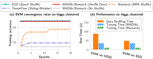
Figure 1: The convergence rate and performance of SVM on the clustered higgs dataset with different data shuffling strategies. (a) Today’s SGD systems over secondary storage, including in-DB ML solutions (e.g., MADlib and Bismarck) and TensorFlow file scanner, are sensitive to clustered data order. (b) Forcing a full data shuffle before training accommodates this clustered data issue, however, introduces large overhead that is often more expensive than training itself.

Existing Landscape and Challenges

Various solutions have been proposed, in the context of both deep learning and in-DB ML systems. TensorFlow provides a shuffling strategy based on a sliding window over the data [18]. In Bismarck [37], the authors suggest a “multiplexed reservoir sampling” (MRS) shuffling strategy, in which two concurrent threads update the same model—one reads data sequentially with reservoir sampling and the other reads from a small, shuffled in-memory buffer. Both significantly improve the SGD convergence rate and have been widely adopted in practice. Despite these efforts, however, they suffer from some shortcomings. As illustrated in Figure 1(a), both strategies proposed by Bismarck and TensorFlow perform suboptimally given a clustered data order. Meanwhile, the idea of shuffling data once before training, i.e., the curve corresponding to “MADlib/Bismarck (Shuffle Once),” can accommodate for such convergence problem but also introduce a significant overhead as shown in Figure 1(b), which is consistent with the observations from previous work [37].

Our Contributions

We are inspired by these previous efforts. In this paper, we ask the following questions:

Can we design an SGD-style algorithm with efficient shuffling strategy that can converge without requiring a full data shuffle? Can we provide a rigorous theoretical analysis on the convergence behavior of such an algorithm? Can we integrate such an algorithm into both deep learning systems and database systems?

In this work, we systematically study these questions and make the following contributions.

C1. An Anatomy and Empirical Study of Existing Algorithms. We start with a systematic evaluation of existing data shuffling strategies for SGD, including (1) Epoch Shuffle, which performs a full shuffle before each epoch, (2) Shuffle Once, (3) No Shuffle, (4) Sliding-Window Shuffle, and (5) MRS Shuffle. We evaluate them in the context of using SGD to train generalized linear models and deep learning models, over a variety of datasets. Our evaluation reveals that existing strategies cannot simultaneously achieve good hardware efficiency (I/O performance) and statistical efficiency (convergence rate and converged accuracy). Specifically, Epoch Shuffle and Shuffle Once achieve the best statistical efficiency, since the data has been fully shuffled; however, their hardware efficiency is suboptimal given the additional shuffle overhead and storage overhead. In contrast, No Shuffle achieves the best hardware efficiency as no data shuffle is required; however, its statistical efficiency suffers as it might converge slowly or even diverge. The other two strategies, Sliding-Window Shuffle and MRS Shuffle, can be viewed as a compromise between Shuffle Once and No Shuffle, which trade statistical efficiency for hardware efficiency. Nevertheless, both strategies suffer in terms of statistical efficiency (Section 3).

C2. A Simple, but Novel, Algorithm with Rigorous Theoretical Analysis. Motivated by the limitations of existing strategies, we propose CorgiPile, a novel SGD-style algorithm based on a two-level hierarchical data shuffle strategy. The main idea is to first sample and shuffle the data at a block level, and then shuffle data at a tuple level within the sampled data blocks, i.e., first sampling data blocks (e.g., a batch of table pages per block in DB), then merging the sampled blocks in a buffer, and finally shuffling the tuples in the buffer for SGD. While this two-level strategy seems quite simple, it can achieve both good hardware efficiency and statistical efficiency. Although the hardware efficiency is easy to understand—accessing random data blocks is much more efficient than accessing random tuples, especially when the block size is large, the statistical efficiency requires some non-trivial analysis. To this end, we further provide a rigorous theoretical study on the convergence behavior.

C3. Implementation, Optimization, and Deep Integration with PyTorch and PostgreSQL. While the benefit of CorgiPile for hardware efficiency is intuitive, its realization requires careful design, implementation, and optimization. Unlike previous in-DB ML systems such as MADlib and Bismarck that integrate ML algorithms using User-Defined Aggregates (UDAs), our technique requires a deeper system integration since it needs to directly interact with the buffer manager. Therefore, we operate at the “physical level” and enable in-DB ML inside PostgreSQL [16] via three new physical operators: BlockShuffle operator, TupleShuffle operator, and SGD operator for our customized SGD implementation. We can then construct an execution plan for the SGD computation by chaining these operators together to form a pipeline, naturally following the built-in Volcano paradigm [39] of PostgreSQL. We also design a double-buffering mechanism to optimize the TupleShuffle operator. For deep learning systems, we extend CorgiPile to work in a parallel/distributed environment, by enhancing the TupleShuffle with multiple buffers.

C4. Extensive Empirical Evaluations. We conduct extensive evaluations to demonstrate the effectiveness of CorgiPile. We first compare CorgiPile with other shuffling strategies in PyTorch using deep learning workloads of image classification and text classification. The results show that CorgiPile achieves similar model accuracy to the best Shuffle Once baseline, whereas other data shuffling strategies suffer from lower accuracy. Specifically, for the ImageNet dataset, CorgiPile is 1.5$\times$ faster than Shuffle Once to converge with 8 GPUs. We then compare the end-to-end performance of our PostgreSQL implementation with two state-of-the-art in-DB ML systems, MADlib and Bismarck. The results again show that CorgiPile achieves comparable model accuracy to the best Shuffle Once baseline, but is significantly faster since it does not require full data shuffle. Other strategies suffer from lower SGD convergence rate on clustered datasets. Overall, CorgiPile can achieve 1.6$\times$-12.8$\times$ speedup compared to MADlib and Bismarck over clustered data. Furthermore, for the datasets ordered by features instead of the label, our CorgiPile still achieves comparable accuracy to the Shuffle Once, whereas No Shuffle suffers from lower accuracy.

Overview

This technical report is organized as follows. We first review the SGD algorithm and its implementation (Section 2). We next empirically study the SGD convergence rate using current state-of-the-art data shuffling strategies (Section 3). We then propose our CorgiPile strategy as well as a theoretical analysis on its convergence (Section 4). We present our implementation of CorgiPile inside PyTorch in Section 5 and inside PostgreSQL in Section 6. We compare the convergence rate and performance of CorgiPile with other baselines in Section 7. We summarize related work in Section 8 and conclude in Section 9.

2 Preliminaries

In this section, we briefly review the standard SGD algorithm and its implementation in the state-of-the-art deep learning and in-DB ML systems.

2.1 Stochastic Gradient Descent (SGD)

Given a dataset with $m$ training examples $\{\mathbf{t}_{i}\}_{i\in[m]}$, e.g., $m$ tuples if the training set is stored as a table in a database, the typical ML task essentially solves an optimization problem that can be cast into minimizing a finite sum over $m$ data examples with respect to model $\mathbf{x}$:

$$F(\mathbf{x})=\frac{1}{m}\sum\nolimits_{i=1}^{m}f_{i}(\mathbf{x}),$$

where each $f_{i}$ corresponds to the loss over each training tuple $\mathbf{t}_{i}$. SGD is an iterative procedure that takes as input hyperparameters such as the learning rate $\eta$ and the maximum number of epochs $S$. It then works as follows.

1. Initialization – Initialize the model $\mathbf{x}$, often randomly.

2. Iterative computation – In each iteration it draws a (batch of) tuple $\mathbf{t}_{i}$, randomly with replacement, computes the stochastic gradient $\nabla f_{i}(\mathbf{x})$ and updates the parameters of model $\mathbf{x}$. In practice, most systems implement a variant, where the random tuples are drawn without replacement [29, 37, 34, 79]. To achieve this, one shuffles all tuples before each epoch and sequentially scans these shuffled tuples. For each tuple, we compute the stochastic gradient and update the model parameters.

3. Termination – The procedure ends when it converges (i.e., the parameters of model $\mathbf{x}$ no longer change) or has attained the maximum number of epochs.

2.2 Deep Learning Systems

Deep learning systems such as PyTorch and TensorFlow are now widely used in industry and academia for AI tasks, including image analysis, natural language processing, speech recognition, etc. These systems usually leverage SGD optimizer or its variants [68, 22, 23] for training deep learning models. To facilitate data loading, these systems classify the datasets into two types, including map-style datasets and iterable-style datasets. Map-style datasets refer to the datasets whose tuples can be randomly accessed given indexes. For example, if an image dataset is stored in an in-memory array as $\langle\texttt{image},\texttt{label}\rangle$ tuples, it is a map-style dataset that can be randomly accessed by the array index. Iterable-style datasets refer to the datasets that can only be accessed in sequence, which is usually used for the datasets that cannot fit in memory. For map-style datasets, it is easy to shuffle them since we only need to shuffle the indexes and access the tuples based on the shuffled indexes. However, this random access usually leads to low I/O performance for secondary storage, as shown in Figure 20 in the Appendix. For iterable-style datasets, PyTorch currently does not provide any built-in shuffling strategies while TensorFlow provides Sliding-Window Shuffle using sliding-window based sampling. As we will see in Section 3, the problem of this shuffling strategy is that it suffers from low accuracy for the clustered dataset.

2.3 In-database Machine Learning Systems

There has been a plethora of work in the past decade focusing on in-DB ML [80, 44, 37, 70, 53, 63, 32, 67, 50, 56, 45, 57, 78, 48]. Most existing in-DB ML systems implement SGD as “User-Defined Aggregates” (UDA) [37, 44]. Each epoch of SGD is done via an invocation of the corresponding UDA function, where the parameters of model $\mathbf{x}$ are treated as the state and updated for each tuple.

To implement the data shuffling step required by SGD, different in-DB ML systems adopt distinct strategies. For example, some systems such as MADlib [44] and DB4ML [46] assume that the training data has already been shuffled, so they do not perform any data shuffling. Other systems, such as Bismarck [37], do not make this assumption. Instead, they either perform a pre-shuffle of the data in an offline manner and then store the shuffled data as a replica in the database, or perform partial data shuffling based on sampling technologies such as reservoir sampling and sliding-window sampling. As we will see in the next section, such partial data shuffling strategies, despite alleviating the computation and storage overhead of the preshuffle strategy, raise new issues regarding the convergence of SGD, since the data is insufficiently shuffled and does not follow the purely random order required.

3 Data Shuffling Strategies for SGD

In this section, we present a systematic analysis of data shuffling strategies used by existing in-DB ML systems. We consider five common data shuffling strategies: (1) Epoch Shuffle, (2) Shuffle Once, (3) No Shuffle, (4) Sliding-Window Shuffle [18], and (5) MRS Shuffle [37]. We use diverse SGD workloads, including generalized linear models such as logistic regression (LR) and support vector machine (SVM), as well as deep learning models such as VGG [72] and ResNet [43].

Experimental Setups. We use the criteo dataset [3] for generalized linear models, and use the cifar-10 image dataset [2] for deep learning. Each dataset has two versions: a shuffled version and a clustered version. In the shuffled version, all tuples are randomly shuffled, whereas in the clustered version all tuples are clustered by their labels. The use of clustered datasets is inspired by similar settings leveraged in [37], with the goal of testing the worst-case scenarios of data shuffling strategies for SGD. For example, the clustered version of criteo dataset has the negative tuples (with “-1” labels) ordered before the positive tuples (with “+1” labels).

3.1 “Shuffle Once” and “Epoch Shuffle”

The Shuffle Once strategy performs an offline shuffle of all data tuples, either in-place or by storing the shuffled tuples as a copy in the database. SGD is then executed over this shuffled copy without any further shuffle during the execution of SGD. Albeit a simple (but costly) idea, it is arguably a strong baseline that many state-of-the-art in-DB ML systems assume when they take as input an already shuffled dataset. For Epoch Shuffle, it shuffles the training set before each training epoch. Therefore, the data shuffling cost of Epoch Shuffle grows linearly with respect to the number of epochs.

Convergence. As illustrated in Figure 2, Shuffle Once can achieve a convergence rate comparable to Epoch Shuffle on both shuffled and clustered datasets, confirming previous observations [37].

Performance. Although Shuffle Once reduces the number of data shuffles to only once, the shuffle itself can be very expensive on large datasets due to the random access of tuples, as we will show in our experiments. Previous work has also reported that shuffling a huge dataset could not be finished in one day [37]. Another problem of Shuffle Once is that, when in-place shuffle is not feasible, it needs to duplicate the data, which can double the space overhead.

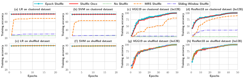
Figure 2: The convergence rates of SGD with different data shuffling strategies, for clustered and shuffled datasets, using the same buffer size (10% of the dataset size) for MRS and Sliding-Window Shuffles.

3.2 “No Shuffle”

The No Shuffle strategy does not perform any data shuffle at all, i.e., the SGD algorithm runs over the given data order in each epoch. Simply running MADlib over a dataset or running PyTorch over IterableDataset picks the No Shuffle strategy.

Convergence. On shuffled data, No Shuffle can achieve comparable convergence rate to Shuffle Once. However, for clustered data, No Shuffle leads to a significantly lower model accuracy. This is not surprising, as SGD relies on a random data order to converge.

Performance. No Shuffle is the fastest among the five data shuffling strategies, as it can always sequentially, instead of randomly, access the data tuples [26].

3.3 “Sliding-Window Shuffle”

The Sliding-Window Shuffle strategy leverages a sliding window to perform partial data shuffling, which is used by TensorFlow [18]. It involves the following steps:

1. Allocate a sliding window and fill tuples as they are scanned.

2. Randomly select a tuple from the window and use it for the SGD computation. The slot of the selected tuple in the window is then filled in by the next incoming tuple.

3. Repeat (2) until all tuples are scanned.

Convergence. As illustrated in Figure 2, for clustered datasets, Sliding-Window Shuffle can achieve higher model accuracy than No Shuffle but lower accuracy than Shuffle Once when SGD converges. The reason is that this strategy shuffles the data only partially. For two data examples $\mathbf{t}_{i}$ and $\mathbf{t}_{j}$ where $\mathbf{t}_{i}$ is stored much earlier than $\mathbf{t}_{j}$ ($i\ll j$), it is likely that $\mathbf{t}_{i}$ is still selected before $\mathbf{t}_{j}$. As a result, on the clustered datasets used in our study, negative tuples are more likely to be selected (for SGD) before positive ones, which distorts the training data seen by SGD and leads to low model accuracy.

Performance. Sliding-Window Shuffle can achieve I/O performance comparable to No Shuffle, as it also only needs to sequentially access the data tuples with limited additional CPU overhead to maintain and sample from the sliding window.

3.4 “Multiplexed Reservoir Sampling Shuffle”

Multiplexed Reservoir Sampling (MRS) Shuffle uses two concurrent threads to read tuples and update a shared model [37]. The first thread sequentially scans the dataset and performs reservoir sampling. The sampled (i.e., selected) tuples are stored in a buffer $B_{1}$ and the dropped (i.e., not selected) ones are used for SGD. The second thread loops over the sampled tuples using another buffer $B_{2}$ for SGD, where tuples are simply copied from the buffer $B_{1}$.

Convergence. As illustrated in Figure 2, MRS Shuffle achieves higher accuracy than Sliding-Window Shuffle but lower accuracy than Shuffle Once when SGD converges. The reason is quite similar to that given to Sliding-Window Shuffle, as the shuffle based on reservoir sampling is again partial and therefore is insufficient when dealing with clustered data. Specifically, the order of the dropped tuples is also generally increasing, i.e., if $i\ll j$, $\mathbf{t}_{i}$ is likely to be processed by SGD before $\mathbf{t}_{j}$. Moreover, looping over the sampled tuples may lead to suboptimal data distribution—the sampled tuples in the looping buffer $B_{2}$ may be used multiple times, which can cause data skew and thus decrease the model accuracy.

Performance. MRS Shuffle is fast, as the first thread only needs to sequentially scan the tuples for reservoir sampling. It is slightly slower than Sliding-Window Shuffle and No Shuffle, as there is a second thread that loops over the buffered tuples.

3.5 Analysis and Summary

Table 1: A Summary of Different Shuffling Strategies, where bold fonts represent the “ideal” scenario. We assume all methods that require an in-memory buffer have reasonably large buffer size, e.g., 1%-10% of the dataset size.

Shuffling Strategy	Convergence Behavior	I/O Perf.	In-memory buffer	Additional Disk Space
No Shuffle	Slow; Lower Accuracy	Fast	No	No
Epoch Shuffle	Fast; High Accuracy	Slow	Yes	2$\times$ data size
Shuffle Once	Fast; High Accuracy	Slow	Yes	2$\times$ data size
MRS Shuffle [37]	Worse than Shuffle Once	Fast	Yes	No
Sliding-Window [18]	Worse than Shuffle Once	Fast	Yes	No
CorgiPile	Comparable to Shuffle Once	Fast	Yes	No

Table 1 summarizes the characteristics of different data shuffling strategies. As discussed, the effectiveness of data shuffling strategies for SGD largely depends on two somewhat conflicting factors, namely, (1) the degree of data randomness of the shuffled tuples and (2) the I/O efficiency when scanning data from disk. There is an apparent trade-off between these two factors:

• The more random the tuples are, the better the convergence rate of SGD is. Epoch Shuffle introduces data randomness at the highest level, but is too expensive to implement in in-DB ML systems. Shuffle Once also introduces significant data randomness, which is usually the best practice in terms of SGD convergence for in-DB ML systems.

• A higher degree of randomness implies more random disk accesses and thus lower I/O efficiency. As a result, the No Shuffle strategy is the best in terms of I/O efficiency.

The other strategies (Sliding-Window and MRS) try to sacrifice data randomness for better I/O efficiency, leaving room for improvement.

Example 1.

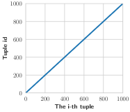
(a) No Shuffle

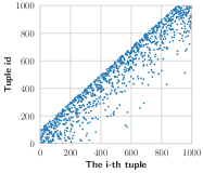
(b) Sliding-Window Shuffle

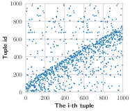
(c) MRS Shuffle

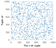
(d) Full Shuffle (ideal)

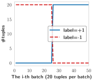
(e) No Shuffle

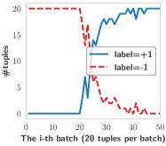
(f) Sliding-Window Shuffle

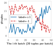
(g) MRS Shuffle

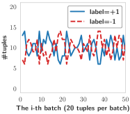
(h) Full Shuffle (ideal)

Figure 3: The tuple id distribution (a-d) and the corresponding label distribution (e-h) of data shuffling strategies. Tuple id denotes the tuple position after shuffling. #tuple denotes the number of negative/positive tuples in every 20 tuples shuffled.

To better understand these issues, consider a clustered dataset with 1,000 tuples, each of which has a tuple_id and a label, where tuple_id of the $i$-th tuple is $i$. The first 500 tuples are negative and the next 500 tuples are positive. Figure 3 plots the distributions of tuple_id and corresponding labels after Sliding-Window and MRS Shuffle, and compare them with the ideal distributions from a full shuffle. Specifically, the tuple_id distribution illustrates the positions of the tuples after shuffling, whereas the label distribution illustrates the number of negative/positive tuples in every 20 tuples shuffled.

We can observe that Sliding-Window results in a “linear”-shape distribution of the tuple_id after shuffling, as shown by Figure 3(b), which suggests that the tuples are almost not shuffled. The corresponding label distribution in Figure 3(f) further confirms this, where almost all negative labels still appear before positive ones after shuffling. Similar patterns can be observed for MRS in Figures 3(c) and 3(g), though MRS has improved over Sliding-Window. In summary, the data randomness achieved by Sliding-Window or MRS is far from the ideal case, as shown in Figures 3(d) and 3(h).

4 CorgiPile

As illustrated in the previous section, data shuffling strategies used by existing systems can be suboptimal when dealing with clustered data. Although recent efforts have significantly improved over baseline methods, there is still large room for improvement. Inspired by these previous efforts, we present a simple but novel data shuffling strategy named CorgiPile. The key idea of CorgiPile lies in the following two-level hierarchical shuffling mechanism:

We first randomly select a set of blocks (each block refers to a set of contiguous tuples) and put them into an in-memory buffer; we then randomly shuffle all tuples in the buffer and use them for SGD.

Despite its simplicity, CorgiPile is highly effective. In terms of hardware efficiency, when the block size is large enough (e.g., 10MB+), a random access on the block level can be as efficient as a sequential scan, as shown in the I/O performance test on HDD and SSD in Appdenx A. In terms of statistical efficiency, as we will show, given the same buffer size, CorgiPile converges much better than Sliding-Window and MRS. Nevertheless, both the convergence analysis and its integration into PyTorch and PostgreSQL are non-trivial. In the following, we first describe the CorgiPile algorithm precisely and then present a theoretical analysis on its convergence behavior.

Notations and Definitions. The following is a list of notations and definitions that we will use:

• $\|\cdot\|$: the $\ell_{2}$-norm for vectors and the spectral norm for matrices;

• $\lesssim$: For two arbitrary vectors $a,g$, we use $a_{s}\lesssim g_{s}$ to denote that there exists a certain constant $C$ that satisfies $a_{s}\leq Cg_{s}$ for all $s$;

• $N$, the total number of blocks ($N\geq 2$);

• $n$, the buffer size (i.e., the number of blocks kept in the buffer);

• $b$, the size (number of tuples) of each data block;

• $B_{l}$, the set of tuple indices in the $l$-th block ($l\in[N]$ and $|B_{l}|=b$);

• $m$, the number of tuples for the finite-sum objective ($m=Nb$);

• $f_{i}(\cdot)$, the function associated with the $i$-th tuple;

• $\nabla F(\cdot)$ and $\nabla f_{i}(\cdot)$, the gradients of the functions $F(\cdot)$ and $f_{i}(\cdot)$;

• $H_{i}(\cdot):=\nabla^{2}f_{i}(\cdot)$, the Hessian matrix of the function $f_{i}(\cdot)$;

• $\mathbf{x}^{*}$, the global minimizer of the function $F(\cdot)$;

• $\mathbf{x}^{s}_{k}$, the model $\mathbf{x}$ in the $k$-th iteration at the $s$-th epoch;

• $\mu$-strongly convexity: function $F(\mathbf{x})$ is $\mu$-strongly convex if $\forall\mathbf{x},\mathbf{y}$,

  $$F(\mathbf{x})\geq F(\mathbf{y})+\left\langle\mathbf{x}-\mathbf{y},\nabla F(\mathbf{y})\right\rangle+\frac{\mu}{2}\|\mathbf{x}-\mathbf{y}\|^{2}.$$ (1)

4.1 The CorgiPile Algorithm

Algorithm 1 CorgiPile Algorithm

1:  Input: $N$ blocks with $m$ total tuples, total epochs $S$ ($S\geq 1$), $a\geq 1$, $F(\cdot)=\frac{1}{m}\sum_{i=1}^{m}f_{i}(\cdot)$.

2:  Initialize $\mathbf{x}^{0}_{0}$;

3:  for $s=0,\cdots,S$ do

4:     Randomly pick $n$ blocks without replacement, each containing $b$ tuples. Load these blocks into the buffer;

5:     Shuffle tuple indices among all $n$ blocks in the buffer and obtain the permutation $\boldsymbol{\psi}_{s}$;

6:     for $k=1,...,bn$ do

7:        Update $\mathbf{x}^{s}_{k}=\mathbf{x}^{s}_{k-1}-\eta_{s}\nabla f_{\psi_{s}(k)}\left(\mathbf{x}^{s}_{k-1}\right)$;

8:     end for

9:     $\mathbf{x}^{s+1}_{0}=\mathbf{x}^{s}_{bn}$;

10:  end for

11:  Return $x_{bn}^{S}$;

Algorithm 1 illustrates the details of CorgiPile. At each epoch (say, the $s$-th epoch), CorgiPile runs the following steps:

1. (Sample) Randomly sample $n$ blocks out of $N$ data blocks without replacement and load the $n$ blocks into the buffer. Note that we use sample without replacement to avoid visiting the same tuple multiple times for each epoch, which can converge faster and is a standard practice in most ML systems [27, 29, 40, 42, 37].

2. (Shuffle) Shuffle all tuples in the buffer. We use $\boldsymbol{\psi}_{s}$ to denote an ordered set, whose elements are the indices of the shuffled tuples at the $s$-th epoch. The size of $\boldsymbol{\psi}_{s}$ is $bn$, where $b$ is the number of tuples per block. $\boldsymbol{\psi}_{s}(k)$ is the $k$-th element in $\boldsymbol{\psi}_{s}$.

3. (Update) Perform gradient descent by scanning each tuple with the shuffle indices in $\boldsymbol{\psi}_{s}$, yielding the updating rule

   $$\mathbf{x}^{s}_{k}=\mathbf{x}^{s}_{k-1}-\eta_{s}\nabla f_{\boldsymbol{\psi}_{s}(k)}\left(\mathbf{x}^{s}_{k-1}\right),$$

   where $\nabla f_{\boldsymbol{\psi}_{s}(k)}(\cdot)$ is the gradient function averaging the gradients of all samples in the tuples indexed by $\boldsymbol{\psi}_{s}(k)$, and $\eta_{s}$ is the learning rate for gradient descent at the epoch $s$. The parameter update is performed for all $k=1,...,bn$ in one epoch.

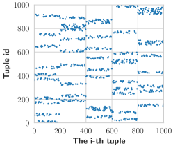
(a) Tuple id distribution of CorgiPile

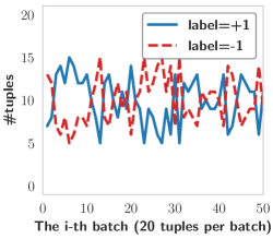
(b) Label distribution of CorgiPile

Figure 4: The tuple id/label distribution of CorgiPile.

Intuition behind CorgiPile. Before we present the formal theoretical analysis, we first illustrate the intuition behind CorgiPile, following the same example used in Section 3.5.

Example 2.

Consider the same settings as those in Example 1. Recall that CorgiPile contains both block-level and tuple-level shuffles. Suppose that the block-level shuffle generates a random order of blocks as {b20, b8, b45, b0, …} and the buffer can hold 10 blocks. The tuple-level shuffle will put the first 10 blocks into the buffer, whose tuple_ids are {b20[400, 419], b8[160, 179], b45[900, 919], b0[0, 19], …}. After shuffling, the buffered tuples will have random tuple_ids in a large non-contiguous interval that is the union of {[0, 19], [160, 179], …, [900, 919]}, as shown in the first 200 tuples in Figure 4(a). The buffered tuples therefore follow a random order closer to what is given by a full shuffle. As a result, the corresponding label distribution, as shown in Figure 4(b), is closer to a uniform distribution.

Performance. While No Shuffle only requires sequential I/Os, our CorgiPile needs to (1) randomly access blocks, (2) copy all tuples in these blocks into a buffer, and (3) shuffle the tuples inside the buffer. Here, random accessing a block means randomly picking a block and reading the tuples of this block from secondary storage (e.g., disk) into memory. If the block size is large enough, the I/O performances of random and sequential accesses are close. CorgiPile incurs additional overheads for buffer copy and in-memory shuffle. However, these I/O overheads can be hidden via standard techniques such as double buffering. As we will show in our experiments on PostgreSQL, the optimized version of CorgiPile only incurs 11.7% additional overhead compared to the most efficient No Shuffle baseline.

4.2 Convergence Analysis

Despite its simplicity, the convergence analysis of CorgiPile is not trivial—even reasoning about the convergence of SGD with sample without replacement is a open question for decades [71, 41, 77, 42], not to say a hierarchical sampling scheme like ours. Luckily, a recent theoretical advancement [42] provides us with the technical language to reason about CorgiPile’s convergence. In the following, we present a novel theoretical analysis for CorgiPile.

Note that in our analysis, one epoch represents going through all the tuples in the sampled $n$ blocks.

Assumption 1.

We make the following standard assumptions, as that in other previous work on SGD convergence analysis [30, 55]:

1. $F(\cdot)$ and $f_{i}(\cdot)$ are twice continuously differentiable.

2. $L$-Lipschitz gradient: $\exists L\in\mathbb{R}_{+}$, $\|\nabla f_{i}(\mathbf{x})-\nabla f_{i}(\mathbf{y})\|\leq L\|\mathbf{x}-\mathbf{y}\|$ for all $i\in[m]$.

3. $L_{H}$-Lipschitz Hessian matrix: $\|H_{i}(\mathbf{x})-H_{i}(\mathbf{y})\|\leq L_{H}\|\mathbf{x}-\mathbf{y}\|$ for all $i\in[m]$.

4. Bounded gradient: $\exists G\in\mathbb{R}_{+}$, $\|\nabla f_{i}(\mathbf{x}_{k}^{s})\|\leq G$ for all $i\in[m]$, $k\in[K-1]$, and $s\in\{0,1\ldots,S\}$.

5. Bounded Variance: $\mathbb{E}_{\xi}[\|\nabla f_{\xi}(\mathbf{x})-\nabla F(\mathbf{x})\|^{2}]=\frac{1}{m}\sum_{i=1}^{m}\|\nabla f_{i}(\mathbf{x})-\nabla F(\mathbf{x})\|^{2}\leq\sigma^{2}$ where $\xi$ is the random variable that takes the values in $[m]$ with equal probability $1/m$.

Factor $h_{D}$. In our analysis, we use the factor $h_{D}$ to characterize the upper bound of a block-wise data variance:

$$\frac{1}{N}\sum_{l=1}^{N}\left\|\nabla f_{B_{l}}(\mathbf{x})-\nabla F(\mathbf{x})\right\|^{2}\leq h_{D}\frac{\sigma^{2}}{b},$$

where $b=|B_{l}|$ is the size of each data block (recall the definition of $b$). Here, $h_{D}$ is an essential parameter to measure the “cluster” effect within the original data blocks. Let’s consider two extreme cases: 1) ($h_{D}=1$) all samples in the data set are fully shuffled, such that the data in each block follows the same distribution; 2) ($h_{D}=b$) samples are well clustered in each block, for example, all samples in the same block are identical. Therefore, the larger $h_{D}$, the more “clustered” the data.

We now present the results for both strongly convex objectives (corresponding to generalized linear models) and non-convex objectives (corresponding to deep learning models) respectively, in order to show the correctness and efficiency of CorgiPile. The proof of the following theorems is at the end of the Appendix.

Strongly convex objective

We first show the result for strongly convex objective that satisfies the strong convexity condition (1).

Theorem 1.

Suppose that $F(\mathbf{x})$ is a smooth and $\mu$-strongly convex function. Let $T=Snb$, that is, the total number of samples used in training and $S\geq 1$ is the number of tuples iterated, and choosing $\eta_{s}=\frac{6}{bn\mu(s+a)}$ where $a\geq\max\left\{\frac{8LG+24L^{2}+28L_{H}G}{\mu^{2}},\frac{24L}{\mu}\right\}$, under Assumption 1, CorgiPile has the following convergence rate

$$\mathbb{E}[F\left(\bar{\mathbf{x}}_{S}\right)-F(\mathbf{x}^{*})]\lesssim(1-\alpha)h_{D}\sigma^{2}\frac{1}{T}+\beta\frac{1}{T^{2}}+\gamma\frac{m^{3}}{T^{3}},$$ (2)

where $\bar{\mathbf{x}}_{S}=\frac{\sum_{s}(s+a)^{3}\mathbf{x}_{s}}{\sum_{s}(s+a)^{3}}$, and

$$\alpha:=\frac{n-1}{N-1},\beta:=\alpha^{2}+(1-\alpha)^{2}(b-1)^{2},\gamma:=\frac{n^{3}}{N^{3}}.$$

Tightness. The convergence rate of CorgiPile is tight in the following sense:

• $\alpha=1$: It means that $n=N$, i.e., all tuples are fetched to the buffer. Then CorgiPile reduces to full-shuffle SGD [42]. In this case, the upper bound in Theorem 1 is $O(1/T^{2}+m^{3}/T^{3})$, which matches the result of the full shuffle SGD algorithm [42].

• $\alpha=0$: It means that $n=1$, i.e., only sampling one block each time. Then CorgiPile is very close to mini-batch SGD (by viewing a block as a mini-batch), except that the model is updated once per data tuple. Ignoring the higher-order terms in (2), our upper bound $O(h_{D}\sigma^{2}/T)$ is consistent with that of mini-batch SGD.

Comparison to vanilla SGD. In vanilla SGD, we only randomly select one tuple from the dataset to update the model. It admits the convergence rate $O(\sigma^{2}/T)$. Comparing to the leading term $(1-\alpha)h_{D}(\sigma^{2}/T)$ in (2) for our algorithm, if $n\gg(h_{D}-1)(N-1)/h_{D}+1$ (for $h_{D}>0$), $(1-\alpha)h_{D}$ will be much smaller than $1$, indicating that our algorithm outperforms vanilla SGD in terms of sample complexity. It is also worth noting that, even if $n$ is small, CorgiPile may still significantly outperform vanilla SGD. Assuming that reading a random single tuple incurs an overhead of $t_{\text{lat}}+t_{\text{t}}$ and reading a block of $b$ tuples incurs an overhead of $t_{\text{lat}}+bt_{\text{t}}$, where $t_{\text{lat}}$ is the “latency” for one read/write operation that does not grow linearly with respect to the amount of data that one reads/writes (e.g., SSD read/write latency or HDD “seek and rotate” time), and $t_{\text{t}}$ is the time that one needs to transfer a single tuple. To reach an error of $\epsilon$, vanilla SGD requires, in physical time,

$$O\left(\frac{\sigma^{2}}{\epsilon}t_{\text{lat}}+\frac{\sigma^{2}}{\epsilon}t_{\text{t}}\right),$$

whereas CorgiPile requires

$$O\left((1-\alpha)\frac{h_{D}}{b}\cdot\frac{\sigma^{2}}{\epsilon}t_{\text{lat}}+(1-\alpha)h_{D}\cdot\frac{\sigma^{2}}{\epsilon}t_{\text{t}}\right).$$

Because $(1-\alpha)\frac{h_{D}}{b}<1$, CorgiPile always provides benefit over vanilla SGD in terms of the read/write latency $t_{\text{lat}}$. When $t_{\text{lat}}$ dominates the transfer time $t_{\text{t}}$, CorgiPile can outperform vanilla SGD even for small buffers.

Non-convex objective

We further conduct an analysis on objectives that are non-convex or satisfy the Polyak-Łojasiewicz condition, which leads to similar insights on the behavior of CorgiPile.

Theorem 2.

Suppose that $F(\mathbf{x})$ is a smooth function. Letting $T=Snb$ be the number of tuples iterated, under Assumption 1, CorgiPile has the following convergence rate:

1. When $\alpha\leq\frac{N-2}{N-1}$, choosing $\eta_{s}=\frac{1}{\sqrt{bn(1-\alpha)h_{D}\sigma^{2}S}}$ and assuming $S\geq\frac{bn(\frac{104}{3}L+\frac{4}{3}L_{H})^{2}}{\sigma^{2}(1-\alpha)h_{D}}$, we have

   $$\frac{1}{S}\sum_{s=1}^{S}\mathbb{E}\|\nabla F(\mathbf{x}_{0}^{s})\|^{2}\lesssim (1-\alpha)^{1/2}\frac{\sqrt{h_{D}}\sigma}{\sqrt{T}}+\beta\frac{1}{T}+\gamma\frac{m^{3}}{T^{\frac{3}{2}}},$$

   where the factors are defined as

   $$\alpha:=\frac{n-1}{N-1},\beta:=\frac{\alpha^{2}}{1-\alpha}\frac{1}{h_{D}\sigma^{2}}+(1-\alpha)\frac{(b-1)^{2}}{h_{D}\sigma^{2}},\gamma:=\frac{n^{3}}{(1-\alpha)N^{3}};$$

2. When $\alpha=1$, choosing $\eta_{s}=\frac{1}{(mS)^{\frac{1}{3}}}$ and assuming $S\geq(\frac{416}{3}L+\frac{16}{3}L_{H})^{3}b^{2}n^{3}/N$, we have

   $$\frac{1}{S}\sum_{s=1}^{S}\mathbb{E}\|\nabla F(\mathbf{x}_{0}^{s})\|^{2}\lesssim\frac{1}{T^{\frac{2}{3}}}+\gamma^{\prime}\frac{m^{3}}{T},$$

   where we define $\gamma^{\prime}:=\frac{n^{3}}{N^{3}}$.

We can apply a similar analysis as that of Theorem  1 to compare CorgiPile with vanilla SGD, in terms of convergence rate, and reach similar insights.

5 Multi-process CorgiPile and the implementation in PyTorch

We have integrated CorgiPile into PyTorch, one of the state-of-the-art deep learning systems. For this integration, the main challenge is to extend CorgiPile to work for the parallel/distributed environment, since deep learning systems usually use multiple processes with multiple GPUs to train models. For example, apart from single-process training, PyTorch also supports multi-process training using the DistributedDataParallel (DDP) mode [8]. In this mode, PyTorch runs multiple processes (typically one process per GPU) in parallel in a single machine or across a number of machines to train models. We call this parallel/distributed multi-process training the multi-process mode.

5.1 Multi-process CorgiPile

We found that our CorgiPile can be naturally extended to work in the multi-process mode, by enhancing the tuple-level shuffle. As mentioned in Section 4.1, CorgiPile contains both block-level shuffle and tuple-level shuffle. For the multi-process mode as shown in Figure 5(a), we can naturally implement block-level shuffle by randomly distributing data blocks into different processes. For the tuple-level shuffle, we can use multi-buffer based shuffling instead of single-buffer based shuffling—in each process we allocate a local buffer to read blocks and shuffle their tuples locally. For the following SGD computation, the deep learning system itself can read the shuffled tuples to perform the forward/backward/update computation as well as gradient/parameter communication/synchronization among different processes. We name this enhanced CorgiPile as multi-process CorgiPile and implement it as a new CorgiPileDataset API in PyTorch as follows. Users just need to initialize the CorgiPileDataset with necessary parameters and then use it as one parameter of the DataLoader. The train() constantly extracts a batch of tuples from DataLoader and performs mini-batch SGD computation on the tuples. We next detail the implementation of multi-process CorgiPile in PyTorch with four steps, and further demonstrate that this multi-process CorgiPile can achieve similar random data order for SGD as that of the single-process CorgiPile in Section 5.2.

    train_dataset = CorgiPileDataset(dataset_path, block_index_path, other_args)
    train_loader = torch.utils.data.DataLoader(train_dataset, other_args)
    train(train_loader, model, other_args)

(1) Block partitioning: The first step is to partition the dataset into blocks. In the parallel/distributed environment, we usually store the dataset on the block-based parallel/distributed file systems such as HDFS [10], Amazon EBS [4], and Lustre [21]. For example, our ETH Euler cluster [7] uses high-performance parallel Lustre file system, which reads/writes data in blocks (by default 4 MB) [13] and does not allow users to store/read massive small files like raw images in a directory. Therefore, for training ImageNet dataset with 1.3 million raw images [11], we need to convert these images into binary data files like widely-used TFRecords [24, 19] and store them in Lustre before training. In addition, for the next block-level shuffle, we need to build a block index to identify the start/end of each block, by using the block information provided by the file system or running indexing tools such as PyTorch-TFRecord library [19] on the dataset. If the dataset itself contains tuple index such as map-style dataset in PyTorch, we can also partition the dataset into blocks according to the tuple index.

(2) Block shuffle: For block shuffle, we just need to let each process randomly pick $\textit{BN}/\textit{PN}$ blocks, where BN is the number of total blocks and PN is the number of total processes. We implement this block shuffle in our CorgiPileDataSet, which uses the dataset path and the block index of all blocks as the input parameters. In the $i$-th process, at the beginning of each epoch, CorgiPileDataSet first shuffles the block index of all blocks and splits it into PN parts, and then only reads the blocks with indexes in the $i$-th part. Since we set the same random seed for each process, the shuffled block indexes in all the processes are the same. Therefore, different processes can obtain different blocks.

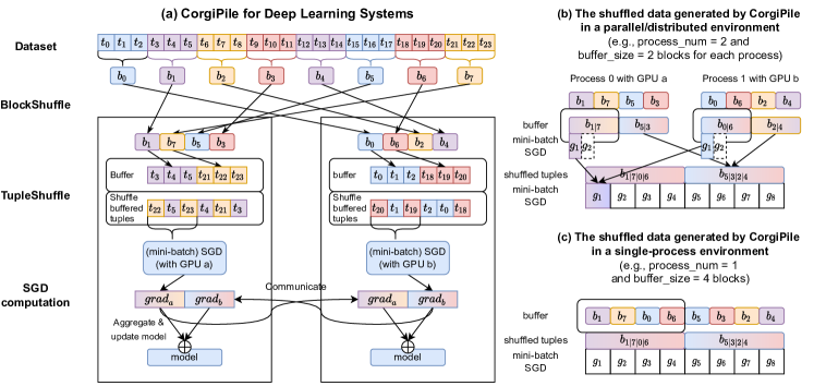
Figure 5: (a) The implementation of CorgiPile in a parallel/distributed environment, e.g., PyTorch with multiple processes and GPUs. (b) The shuffled data generated by CorgiPile in a parallel/distributed environment are similar with (c) the shuffled data generated by CorgiPile in a single-process environment.

(3) Tuple shuffle: For tuple shuffle, each process first allocates a small buffer in memory and then constantly reads the blocks into the buffer. Once the buffer is full, the process will shuffle the buffered tuples. This is also implemented in CorgiPileDataSet, whose iter() reads blocks into a buffer and returns the shuffled tuples one by one to the next SGD computation. Note that the buffer size here is much smaller than that used in the single-process mode. For example, if we set $\textit{buffer}\_\textit{size}=\textit{BS}$ in the single-process mode, we can choose $\textit{buffer}\_\textit{size}=\textit{BS}/\textit{PN}$ for the multi-process mode. We will compare the shuffled data orders of these two modes later.

(4) SGD computation: After the block shuffle and tuple shuffle, each process can perform mini-batch SGD computation on the shuffled tuples. Different from the single-process mode that performs mini-batch SGD on the whole dataset with $\textit{batch}\_\textit{size}=\textit{bs}$, each process in the multi-process mode performs mini-batch SGD on partial dataset with a smaller batch size ($\textit{bs}/\textit{PN}$) and updates the model with gradient synchronization every batch. As shown in Figure 5(a), after each batch, all the processes will synchronize/aggregate the gradients using communication protocols like AllReduce, and then updates the local model. This procedure is executed inside train() of PyTorch, which automatically performs the gradient computation/communication/synchronization and model update every time after reading a batch of tuples from CorgiPileDataset.

5.2 Single-process CorgiPile vs. Multi-process CorgiPile

We found that the generated data order of multi-process CorgiPile is comparable to that of single-process CorgiPile, when using mini-batch SGD. Here, we use a simple example as shown in Figure 5 to demonstrate this. As shown in Figure 5(a), there are two processes and each of them randomly picks 4 blocks from the dataset. Each process can read two blocks into the buffer at once and shuffle their tuples. As a result, as shown in Figure 5(b), the shuffled tuples of process 0 are in sequence from block 1/7 (denoted as $b_{1|7}$) and then from block 5/3. Likewise, the shuffled tuples of process 1 are in sequence from block 0/6 and then from block 2/4. Since PyTorch sequentially performs mini-batch SGD on the first $\textit{batch}\_\textit{size}/\textit{PN}$ tuples of each process (denoted as $g_{1}$ on block 1/7 and block 0/6) and synchronizes their gradients (sums and averages $g_{1}$) every batch, it is the same as performing mini-batch SGD on the first $\textit{batch}\_\textit{size}$ tuples from block 1/7/0/6 (i.e., $g_{1}$ on $b_{1|7|0|6}$). Therefore, from the view of the whole dataset, PyTorch performs mini-batch SGD on the tuples first from block 1/7/0/6 and then from block 5/3/2/4. This is similar to the data order generated by single-process mode in Figure 5(c), where the buffer size is PN times of that of the multi-process mode. Here, the PN is 2 and the buffer can keep 4 blocks at once. In summary, due to block shuffle, multi-buffer based tuple shuffle, and synchronization protocol of mini-batch SGD, multi-process CorgiPile can achieve shuffled data order similar to that of the single-process CorgiPile.

6 Implementation in the Database

We integrate CorgiPile into PostgreSQL. Our implementation provides a simple SQL-based interface for users to invoke CorgiPile, with the following query template:

                    SELECT * FROM table TRAIN BY model WITH params.

This interface is similar to that offered by existing in-DB ML systems such as MADlib [44, 5] and Bismarck [37]. Examples of the params include learning_rate = 0.1, max_epoch_num = 20, and block_size = 10MB. CorgiPile outputs various metrics after each epoch, such as training loss, accuracy, and execution time.

The Need of a Deeper Integration

Unlike existing in-DB ML systems, we choose not to implement our CorgiPile strategy using UDAs. Instead, we choose to integrate CorgiPile into PostgreSQL by introducing physical operators. Is it necessary for such a deeper integration with database system internals, compared to a potential UDA-based implementation without modifying the internals?

While a UDA-based implementation is conceptually possible, it is not natural for CorgiPile, which requires accessing low-level data layout information such as table pages, tuples, and buffers. A deeper integration with database internals makes it much easier to reuse such functionalities that have been built into the core APIs offered by database system internals but not yet have been externally exposed as UDAs. Moreover, such a physical-level integration opens up the door for more advanced optimizations, such as double-buffering that will be illustrated in Section 6.3.

6.1 Design Considerations

As discussed in Section 4.1, CorgiPile consists of three steps: (1) block-level shuffling, (2) tuple-level shuffling, and (3) SGD computation. Accordingly, we design three physical operators, one for each of the three steps:

• BlockShuffle, an operator for randomly accessing blocks;

• TupleShuffle, an operator for buffering a batch of blocks and shuffling their tuples;

• SGD, an operator for the SGD computation.

We then chain these three operators together to form a pipeline, and implement the getNext() method for each operator, following the classic Volcano-style execution model [39] that is also the query execution paradigm of PostgreSQL.

One challenge is the design and implementation of the SGD operator, which requires an iterative procedure that is not typically supported by database systems. We choose to implement it by leveraging the built-in re-scan mechanism of PostgreSQL to reshuffle and reread the data after each epoch.

We store the dataset as a table in PostgreSQL using the schema of $\langle\textit{id},\textit{features\_k}[],\textit{features\_v}[],\textit{label}\rangle$, which is similar to the one used by Bismarck [37]. For sparse datasets, $\textit{features\_k}[]$ indicates which dimensions have non-zero values, and $\textit{features\_v}[]$ refers to the corresponding non-zero feature values. For dense dataset, only $\textit{features\_v}[]$ is used.

Currently, we store the (learned) machine learning model as an in-memory object (a C-style Struct) with an ID in the PostgreSQL’s kernel instead of using UDA. Users can initialize the model hyperparameters via the query. For the inference, users can execute a query as “SELECT table PREDICT BY model ID”, which invokes the learned model for prediction.

6.2 Physical Operators

The control flow of the three operators is shown in Figure 6, which leverages a PostgreSQL’s pull-style dataflow to read tuples and perform the SGD computation. In the following, we assume that the readers are familiar with the structure of PostgreSQL’s operators, e.g., functions such as ExecInit() and getNext().

After parsing the input query, CorgiPile invokes ExecInit() of each operator to initialize their states such as ML models and I/O buffers. At each epoch, the SGD operator pulls tuples from the TupleShuffle operator for SGD computation, which further pulls tuples from the BlockShuffle operator. The BlockShuffle operator is responsible for shuffling blocks and reading their tuples. We now present the implementation of these operators.

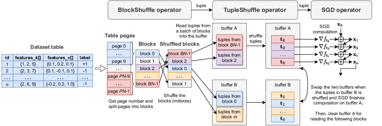
Figure 6: The implementation of CorgiPile with three new operators and the “double-buffering” optimization, in PostgreSQL.

(1) BlockShuffle: This operator first obtains the total number of pages by PostgreSQL’s internal function as RelationGetNumberOfBlocks(). It then computes the number of blocks BN by $\textit{BN}=\textit{page\_num}*\textit{page\_size}/\textit{block\_size}.$ After that, it shuffles the block indices $[0,\dots,\textit{BN}-1]$ and obtains shuffled block ids, where each block corresponds to a batch of contiguous table pages. For each shuffled block id, it reads the corresponding pages using heapgetpage() and returns each fetched tuple to the TupleShuffle operator. The BlockShuffle operator is somewhat similar to PostgreSQL’s Scan operator, although the Scan operator reads pages sequentially instead of randomly.

(2) TupleShuffle: It first allocates a buffer, and then pulls the tuples one by one from the BlockShuffle operator by invoking its ExecTupleShuffle(), i.e., getNext(). Each pulled tuple is transformed to an SGDTuple object, which is then copied to the buffer. Once the buffer is filled, it shuffles the buffered tuples, which is similar to how the Sort operator works in PostgreSQL. After that, the shuffled tuples are returned one by one to the SGD operator.

(3) SGD: It first initializes an ML model in ExecInitSGD() and then executes SGD in ExecSGD(). At each epoch, ExecSGD() pulls tuples from TupleShuffle one by one, and runs SGD computation. Once all tuples are processed, an epoch ends. It then has to reshuffle and reread the tuples for the next epoch, using the re-scan mechanism of PostgreSQL. Specifically, after each epoch, SGD invokes ExecReScan() of TupleShuffle to reset the I/O states of the buffer. It further invokes ExecReScan() of BlockShuffle to reshuffle the block ids. After that, SGD operator can reread shuffled tuples via ExecSGD() for the next epoch. This is similar to the multiple table/index scans in PostgreSQL’s NestedLoopJoin.

6.3 Optimizations

As discussed in Section 4.1, CorgiPile introduces additional overheads for buffer copy and shuffle. To reduce them, we use a double-buffering strategy as shown in Figure 6. Specifically, we launch two concurrent threads for TupleShuffle with two buffers. One write thread is responsible for pulling tuples from BlockShuffle into one buffer and shuffling the buffered tuples; the other read thread is responsible for reading tuples from another buffer and returning them to SGD. The two buffers are swapped once one is full and the other has been consumed by SGD. As a result, the data loading (i.e., block-level and tuple-level shuffling) and SGD computation can be executed concurrently, reducing the overhead.

Table 2: Datasets. The first four are from LIBSVM [3]. For criteo, we extract 98M tuples from the criteo terabyte dataset. For yfcc, we extract 3.6M tuples from the yfcc100m dataset [74]; the outdoor and indoor tuples are marked as negative (-1) and positive (+1). #Tuples like 4.5/0.5M refer to 4.5M tuples for training and 0.5M tuples for testing.

Name	Type	#Tuples	#Features	Size in DB or on disk
higgs	dense	10.0/1.0M	28	2.8 GB
susy	dense	4.5/0.5M	18	0.9 GB
epsilon	dense	0.4/0.1M	2,000	6.3 GB
criteo	sparse	92/6.0M	1,000,000	50 GB
yfcc	dense	3.3/0.3M	4,096	55 GB
ImageNet	image	1.3/0.05M	224*224*3	150 GB
cifar-10	image	0.05/0.01M	3,072	178 MB
yelp-review-full	text	0.65/0.05M	-	600 MB

7 Evaluation

We evaluate CorgiPile on both deep learning and in-DB ML systems. Our goal is to study the statistical and hardware efficiency of CorgiPile when applied to these systems, i.e., whether it can achieve both high accuracy and high performance. For deep learning system, we integrate CorgiPile into PyTorch and compare it with other shuffling strategies, using both image classification and natural language processing workloads. For in-DB ML systems, we compare our PostgreSQL-based implementation with two state-of-the-art systems, Apache MADlib and Bismarck with diverse linear models and datasets. Next, we first evaluate deep learning models in Section 7.2. After that, we evaluate linear models with standard SGD in PostgreSQL in Section 7.3. We further evaluate linear models with mini-batch SGD as well as other types of (continuous, multi-class, and feature-ordered) datasets in PostgreSQL in Section 7.4.

7.1 Experimental Setup

7.1.1 Runtime

For deep learning workloads, we perform them on our ETH Euler cluster [7] as batch jobs. Each job can use maximum 16 CPU cores, 160 GB RAM, and 8 NVIDIA GeForce RTX 2080 Ti GPUs. The datasets are stored in the cluster’s block-based Lustre parallel file system.

For in-DB ML workloads, we perform the experiments on a single ecs.i2.xlarge node in Alibaba Cloud. It has 2 physical cores (4 vCPU), 32 GB RAM, 1000 GB HDD, and 894 GB SSD. The HDD has a maximum 140 MB/s bandwidth, and the SSD has a maximum 1 GB/s bandwidth. Moreover, CorgiPile only uses a single physical core, and we bind the two threads (see Section 6.3) to the same physical core using the “taskset -c” command. We run all experiments in PostgreSQL under CentOS 7.6, and we clear the OS cache before running each experiment.

7.1.2 Datasets

For deep learning, we use both cifar-10 dataset with 10 classes [2] and ImageNet dataset with 1,000 classes [11] for image classification. We also use yelp-review-full dataset [81] with 5 classes for text classification. For in-DB ML, we use a variety of datasets in our evaluation, including dense/sparse and small/large ones as shown in Table 2. The datasets in Table 2 are stored in PostgreSQL for in-DB ML experiments. For both deep learning and in-DB ML, we focus on the evaluation over the clustered datasets, since SGD with various data shuffling strategies can achieve comparable convergence rates on the shuffled datasets, as shown in Figure 2.

7.1.3 Models and Parameters

For the evaluation on deep learning system, we perform the classical VGG19 and ResNet18 models on the cifar-10 dataset, and perform more complex ResNet50 model on the ImageNet dataset. We also perform the classical HAN [76] and TextCNN [51] models for text classification, with pre-trained word embeddings [64] on the yelp-review-full dataset. For the evaluation on in-DB ML systems, we mainly train two popular generalized linear models, logistic regression (LR) and support vector machine (SVM), that are also supported by Bismarck and MADlib. We briefly report the evaluation results for other liner models such as linear regression and softmax regression, which are currently only supported by MADlib.

Currently, Bismarck and MADlib only support two of the baseline data shuffling strategies, namely, No Shuffle and Shuffle Once, which we compare our PostgreSQL-based implementation against. Note that the code of MRS Shuffle has not been released by Bismarck yet. Therefore, we leave it out of our end-to-end comparisons. Instead, we implemented MRS Shuffle by ourselves in PyTorch and compare with it when we discuss the convergence behavior of different data shuffling strategies (like Figure 12).

The model hyperparameters include the learning rate, the decay factor, and the maximum number of epochs. By default, we use an exponential learning rate decay with 0.95. We set the number of epochs to 20 for in-DB ML and 50 for deep learning models. Only for ResNet50 on ImageNet, we set the epoch number to 100 and decay the learning rate every 30 epochs, following the official PyTorch-ImageNet code [12]. We use grid search to tune the best learning rate from {0.1, 0.01, 0.001}. For in-DB ML, we use the same initial parameters and hyperparameters among the compared systems, including MADlib, Bismarck, and CorgiPile.

7.1.4 Settings of CorgiPile

CorgiPile has two more parameters, i.e., the buffer size and the block size. We experiment with a diverse range of buffer sizes in {1%, 2%, 5%, 10%} and the block size is chosen in {2MB, 10MB, 50MB}. We always use the same buffer size (by default 10% of the whole dataset size) for Sliding-Window Shuffle, MRS Shuffle, and our CorgiPile.

7.1.5 Settings of PostgreSQL

For PostgreSQL, we set the work_mem to be the maximum RAM size and tune shared_buffers. Note that PostgreSQL can further compress high-dimensional datasets using the so-called TOAST [17] technology, which tries to compress large field value or break it into multiple physical rows. For our dense epsilon and yfcc datasets with 2,000+ dimensions, PostgreSQL uses TOAST to compress their features_v columns.

7.2 Evaluation with Deep Learning System

CorgiPile is a general data shuffling strategy for any SGD implementation. To understand its impact on deep learning systems and workloads, we implement the CorgiPile strategy as well as others in PyTorch and compare them using deep learning models, for both image classification and text classification. In the following parts, we first evaluate the end-to-end performance and convergence rate of CorgiPile on the ImageNet dataset. We then study the convergence rate of CorgiPile and compare it with others on other datasets, including cifar-10 and yelp-review-full. Furthermore, we explore whether CorgiPile can work on other first-order optimization methods such as Adam [52] in Section 7.2.3.

7.2.1 Performance comparison

To evaluate the performance of CorgiPile in PyTorch, we perform ResNet50 model on ImageNet dataset, which has 1.3 million images in 1,000 classes. We run this experiment using multi-process CorgiPile with 8 GPUs and 16 CPU cores in our ETH Euler cluster. We evaluate two different block sizes (5MB and 10MB that are about 50 and 100 images per block), as our Euler cluster reads data in terms of 4MB+ blocks. The batch size is set to $512$ images, so each process performs SGD computation on $512/8=64$ images per batch. The buffer size of each process is 1.25% of the whole dataset, thus the total buffer size of all processes is 10% of the whole dataset. The number of data loading threads for each process is set to two, since we have twice as many CPU cores as GPUs. The learning rate is initialized as 0.1 and is decayed every 30 epochs.

Figure 7 illustrates the end-to-end execution time of ResNet50 model on the large ImageNet dataset, using different shuffling strategies. We report both the Top 1 and Top 5 accuracy. From Figure 7(a) and 7(b), we can observe that CorgiPile is 1.5$\times$ faster than Shuffle Once to converge and the converged accuracy of CorgiPile is similar to that of Shuffle Once. The main reason of the slowness of Shuffle Once is that it needs about 8.5 hours to shuffle the large ($\sim$150 GB) ImageNet dataset and store the shuffled dataset in our Euler cluster. In contrast, CorgiPile eliminates this long data shuffling time. The second reason is that our CorgiPile has limited per-epoch overhead. Although CorgiPile has block shuffle and tuple shuffle overhead, the per-epoch time of CorgiPile with 5MB or 10MB block is only $\sim$15% longer than that of the fastest No Shuffle baseline. The reason is that CorgiPile reads data in terms of blocks which is comparable to sequential read on block-based parallel file system.

For the convergence rate comparison as shown in Figure 7(c) and  7(d), we can see that the convergence rates of both CorgiPile with 5 MB block and CorgiPile with 10 MB block are comparable to that of Shuffle Once. Although CorgiPile with 10 MB block has a bit lower convergence rate than Shuffle Once in the first 30 epochs, it can catch up with Shuffle Once in the following epochs and converges to the similar accuracy as Shuffle Once. In contrast, the converged accuracy of No Shuffle is close to $0\%$.

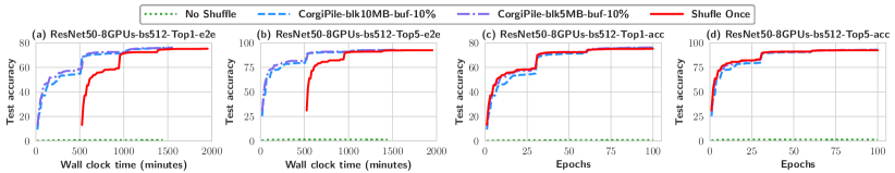
Figure 7: The convergence rates of ResNet50 with different data shuffling strategies, for the clustered ImageNet dataset. TopN refers to the Top-N accuracy.

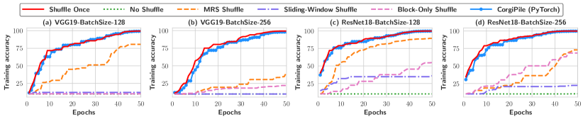
Figure 8: The convergence rates of deep learning models with different data shuffling strategies and batch sizes, for the clustered 10-class cifar-10 image dataset.

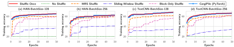
Figure 9: The convergence rates of deep learning models with different data shuffling strategies and batch sizes, for the clustered 5-class yelp-review-full text dataset.

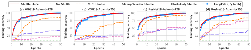
Figure 10: The convergence rates of deep learning models with different data shuffling strategies and batch sizes, using Adam instead of SGD for the clustered cifar-10 image dataset.

7.2.2 Convergence rate comparison

We perform PyTorch with CorgiPile and other strategies on cifar-10 image dataset and yelp-review-full dataset using a single GPU. The cifar-10 dataset contains 50,000 training images in 10 classes, while the yelp-review-full dataset has 650,000 reviews (text messages) in 5 classes.

For the image classification, Figure 8 illustrates the convergence rates of VGG19 and ResNet18 models on the clustered cifar-10 dataset, with different shuffling strategies and different batch sizes (128 and 256). The buffer size is $10\%$ of the whole dataset and the block size is set to 100 images per block. This figure shows that CorgiPile achieves comparable convergence rate and accuracy to the Shuffle Once baseline, whereas other strategies suffer from lower accuracy due to the partially random order of the shuffled tuples. Specifically, the Sliding-Window Shuffle used by TensorFlow only performs better than No Shuffle, and suffers from large (50%+) accuracy gap with Shuffle Once and CorgiPile.

For the text classification, Figure 9 shows the convergence results of classical HAN [76] and TextCNN [51] models with pre-trained word embeddings [64] on the clustered yelp-review-full dataset [81] with different batch sizes (128 and 256). The buffer size is still $10\%$ of the whole dataset and the block size is set to 1,000 reviews per block. Again, CorgiPile achieves similar convergence rate and accuracy to the Shuffle Once baseline, whereas other strategies converge to lower accuracy. Specifically, No Shuffle only achieves about $20\%$ accuracy for the two models, and the Sliding-Window Shuffle used by TensorFlow only achieves about $40\%$ accuracy. MRS Shuffle converges faster and better than them but still suffers from lower accuracy than the Shuffle Once baseline.

The above results indicate that CorgiPile can achieve both good statistical efficiency and hardware efficiency for deep learning models on non-convex optimization problems. When integrated to PyTorch, CorgiPile is 1.5$\times$ faster than the Shuffle Once baseline on the large ImageNet dataset in our experiments.

7.2.3 Beyond SGD optimizer

Although our work focuses on the most popular SGD optimizer, we are confident that CorgiPile can also be used in other optimizers, such as more complex first-order optimizers like Adam [52].

Here, we further perform VGG19 and ResNet18 models on the clustered cifar-10 dataset using Adam instead of SGD. Figure 10 shows the convergence results with different batch sizes (128 and 256). The result of the convergence rate comparison is similar to that of SGD in Figure 8. Our CorgiPile still achieves comparable convergence rate and accuracy to the best Shuffle Once baseline, whereas other shuffling strategies suffer from lower accuracy.

7.3 Evaluation on SGD with In-DB ML Systems

Figure 11: The end-to-end execution time of SGD with different data shuffling strategies in PostgreSQL, for clustered datasets on HDD and SSD. We only show the first 5 epochs for Shuffle Once and CorgiPile, since they converge in 1-3 epochs.

For in-DB ML, we first evaluate CorgiPile in terms of the end-to-end execution time. The compared systems include No Shuffle and Shuffle Once strategies in MADlib and Bismarck, as well as a simpler version of our CorgiPile named Block-Only Shuffle, to see how CorgiPile behaves without tuple-level shuffle. We then analyse the convergence rates, in comparison with other strategies, including MRS Shuffle and Sliding-Window Shuffle. We finally study the overhead of CorgiPile by comparing the per-epoch execution time of CorgiPile with the fastest No Shuffle baseline.

In the following, we set the buffer size to $10\%$ of the whole dataset and block size to 10 MB for all methods. We report a sensitivity analysis on the impact of buffer sizes and block sizes in Section 7.3.4.

7.3.1 End-to-end Execution Time

Figure 11 presents the end-to-end execution time of SGD for in-DB ML systems, for clustered datasets on both HDD and SSD. The end-to-end execution time includes: (1) the time for shuffling the data, i.e., Shuffle Once needs to perform a full data shuffle before SGD starts running; (2) the data caching time, i.e., the time spent on loading data from disk to the OS cache during the first epoch; and (3) the execution time of all epochs.

From Figure 11, we can observe that CorgiPile converges the fastest among all systems, and simultaneously achieves comparable converged accuracy to the best Shuffle Once baseline, usually within 1-3 epochs because of the large number of data tuples. Compared to Shuffle Once in MADlib and Bismarck, CorgiPile converges 2.9$\times$-12.8$\times$ faster than MADlib and 2$\times$-4.7$\times$ faster than Bismarck, on HDD and SSD. This is due to the eliminated data shuffling time. For example, for the clustered yfcc dataset on HDD, CorgiPile can converge in 16 minutes, whereas Shuffle Once in Bismarck needs 50 minutes to shuffle the dataset and another 15 minutes to execute the first epoch (to converge). That is, when CorgiPile converges, Shuffle Once is still performing data shuffling. For other datasets like criteo and epsilon, similar observations hold. Moreover, data shuffling using ORDER BY RANDOM() in PostgreSQL, as implemented by Shuffle Once in MADlib/Bismarck, requires 2$\times$ disk space to generate and store the shuffled data. Therefore, CorgiPile is both more efficient and requires less space.

MADlib is slower than Bismarck given that it performs more computation on some auxiliary statistical metrics and has less efficient implementation [46]. Moreover, for high-dimensional dense datasets, such as epsilon and yfcc, MADlib LR cannot finish even a single epoch within 4 hours, due to some expensive matrix computations on a metric named stderr. MADlib’s SVM implementation does not have this problem and can finish its execution on high-dimensional dense datasets. In addition, MADlib currently does not support training LR/SVM on sparse datasets such as criteo dataset.

7.3.2 Convergence rate comparison

Table 3: The final training and testing accuracy of Shuffle Once (SO) and CorgiPile.

	LR (SO $|$ CorgiPile)		SVM (SO $|$ CorgiPile)
Dataset	Train acc. (%)	Test acc. (%)	Train acc. (%)	Test acc. (%)
higgs	64.04 $|$ 64.07	64.04 $|$ 64.06	64.11 $|$ 64.22	63.93 $|$ 63.95
susy	78.61 $|$ 78.54	78.69 $|$ 78.66	78.61 $|$ 78.66	78.73 $|$ 78.66
epsilon	90.02 $|$ 90.01	89.77 $|$ 89.74	90.12 $|$ 90.11	89.81 $|$ 89.80
criteo	78.97 $|$ 78.91	78.77 $|$ 78.69	78.31 $|$ 78.41	78.45 $|$ 78.44
yfcc	96.43 $|$ 96.38	96.14 $|$ 96.11	96.35 $|$ 96.31	96.23 $|$ 96.20

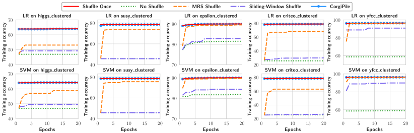
Figure 12: The convergence rates of LR and SVM with different shuffling strategies for clustered datasets.

For all datasets inspected, the gap between Shuffle Once and CorgiPile is below 1% for the final training/testing accuracy, as shown in Table 3. We attribute this to the fact that CorgiPile can yield good data randomness in each epoch of SGD (Section 4.2). No Shuffle results in the lowest accuracy when SGD converges, as illustrated in Figure 11. The Block-Only Shuffle baseline, where we simply omit tuple-level shuffle in CorgiPile, can achieve higher accuracy than No Shuffle but lower accuracy than Shuffle Once. The reason is that Block-Only Shuffle can only yield a partially random order, and the tuples in each block can all be negative or positive for the clustered data.

Since MRS Shuffle and Sliding-Window Shuffle are not available in the current MADlib/Bismarck, we use our own implementations (in PyTorch) and compare their convergence rates. Figure 12 shows the convergence rates of all strategies, where Sliding-Window, MRS, and CorgiPile all use the same buffer size (10% of the whole dataset). As shown in Figure 12, Sliding-Window Shuffle suffers from lower accuracy, whereas MRS Shuffle only achieves comparable accuracy to Shuffle Once on yfcc but suffers on the other datasets.

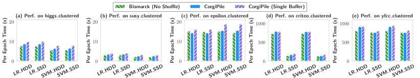
Figure 13: The average per-epoch time of SGD with Bismarck (No Shuffle), CorgiPile, and CorgiPile with single buffer in PostgreSQL, for clustered datasets on HDD and SSD. It shows that CorgiPile is up to 11.7% slower than the fastest No Shuffle.

7.3.3 Per-epoch Overhead

To study the overhead of CorgiPile, we compare its per-epoch execution time with the fastest No Shuffle baseline, as well as the single-buffer version of CorgiPile, as shown in Figure 13. We make the following three observations.

• For small datasets with in-memory I/O bandwidth, the average per-epoch time of CorgiPile is comparable to that of No Shuffle.

• For large datasets with disk I/O bandwidth, the average per-epoch time of CorgiPile is up to $\sim$1.1$\times$ slower than that of No Shuffle, i.e., it incurs at most an additional 11.7% overhead, due to buffer copy and tuple shuffle.

• By using double-buffering optimization, CorgiPile can achieve up to 23.6% shorter per-epoch execution time, compared to its single-buffering version.

The above results reveal that CorgiPile with double-buffering optimization can introduce limited overhead (11.7% longer per-epoch execution time), compared to the best No Shuffle baseline.

7.3.4 Sensitivity Analysis

We next study the effects of different buffer sizes, I/O bandwidths, and block sizes for CorgiPile.

The effects of buffer size. Figure 14(a) reports the convergence behavior of CorgiPile on the two largest datasets with different buffer sizes: 1%, 2%, and 5% of the dataset size. We see that CorgiPile only requires a buffer size of 2% to maintain the same convergence behavior as Shuffle Once. With a 1% buffer, it only converges slightly slower than Shuffle Once, but achieves the same final accuracy. On the other hand, as discussed in previous sections, Sliding-Window Shuffle and MRS Shuffle achieve a much lower accuracy even when given a much larger buffer (10%).

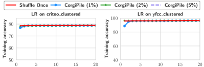
(a) CorgiPile’s convergence with varying buffer sizes.

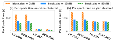
(b) Per-epoch time of CorgiPile with varying block sizes.

Figure 14: The effects of buffer size and block size on CorgiPile.

The effects of I/O bandwidth. As shown in Figure 13, for smaller datasets such as higgs, susy, and epsilon, CorgiPile on HDD and CorgiPile on SSD achieve the similar per-epoch times, since these datasets have been cached in memory after the first epoch. For larger datasets such as criteo, CorgiPile is faster on SSD than HDD, as expected. Interestingly, for yfcc, CorgiPile achieves similar performance on both HDD and SSD. The reason is that the TOAST compression on yfcc slows down data loading to only $\sim$130 MB/s on both SSD and HDD, whereas it achieves $\sim$700/130 MB/s on SSD/HDD for criteo without this compression. The same observation holds for No Shuffle on HDD/SSD for these datasets.

The effects of block size. We vary the block size in $\{$2MB, 10MB, 50MB$\}$ on the large criteo and yfcc datasets. Figure 14(b) shows that the per-epoch time decreases as the block size increases from 2MB to 50MB, due to the higher I/O bandwidth (throughput). However, the time difference between 10MB and 50MB is limited (under 10%), because using 10MB has achieved the highest possible I/O bandwidth (130 MB/s on HDD). In practice, we recommend users to choose the smallest block size that can achieve high-enough I/O throughput, using I/O test commands such as “fio” in Linux.

7.3.5 Performance comparison with PyTorch

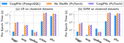
Figure 15: The per-epoch time comparison between in-DB CorgiPile and PyTorch on SSD.

To further understand the performance gap between our in-DB CorgiPile and the start-of-the-art PyTorch outside DB, we compare them in two ways.

(1) CorgiPile in PostgreSQL vs. PyTorch: Figure 15 shows the per-epoch time comparison between CorgiPile in PostgreSQL and PyTorch with No Shuffle. For PyTorch, we load small datasets into memory before training to reduce the I/O overhead, and store the large criteo and yfcc datasets on disk. The comparison results in Figure 15 show that our in-DB CorgiPile is 2-16$\times$ faster than PyTorch on higgs, susy, criteo, and yfcc datasets. We speculate that this is because PyTorch has high overhead of Python-C++ invocations of forward/backward/update functions for each tuple, and these datasets have a large number (3-92 millions) of tuples. Only for the epsilon dataset, PyTorch is 2-3$\times$ faster than CorgiPile. The reason is that this dataset is compressed in DB by TOAST [17]. CorgiPile needs to decompress each tuple, while PyTorch directly computes on the in-memory uncompressed data.

(2) Outside DB: Figure 15 shows that PyTorch with CorgiPile introduces small (up to 16%) overhead compared to PyTorch with No Shuffle, which is consistent with what we observed in DB.

7.4 Evaluation on Mini-Batch SGD and other types of datasets with In-DB ML Systems

In the previous experiments, we focus on the standard SGD algorithm, which updates the model per tuple. Since it is also common to use mini-batch SGD, we implement mini-batch SGD for CorgiPile, Once Shuffle, No Shuffle, and Block-Only Shuffle, using our in-DB operators in PostgreSQL. Since MADlib and Bismarck currently do not support mini-batch SGD for linear models, we compare these shuffling strategies based on our PostgreSQL implementations.

7.4.1 Mini-batch LR and SVM models

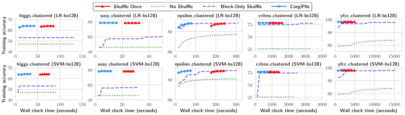
Figure 16: The end-to-end execution time of LR and SVM using mini-batch SGD (batch_size = 128) in PostgreSQL, for clustered datasets on SSD.

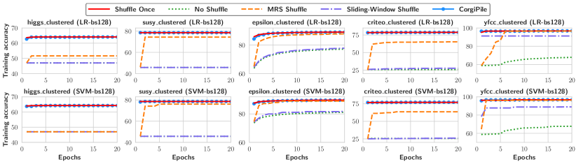
Figure 17: The convergence rates of LR and SVM using mini-batch SGD (batch_size = 128), for clustered datasets.

We first perform LR and SVM using mini-batch SGD on the clustered datasets. Figure 16 illustrates the end-to-end execution time of these two models in PostgreSQL on SSD. The result is similar to that of the standard SGD. Our CorgiPile achieves comparable convergence rate and accuracy to Shuffle Once but 1.7-3.3$\times$ faster than it to converge. Other strategies like No Shuffle and Block-Only Shuffle suffer from either lower converged accuracy or lower convergence rate.

Figure 17 demonstrates the convergence rates of different shuffling strategies with batch_size = 128. From this figure, we can see that Sliding-Window Shuffle and MRS Shuffle have convergence rate or accuracy gap with CorgiPile and Shuffle Once, for clustered datasets. Only for yfcc dataset, MRS Shuffle can converge to the similar accuracy to CorgiPile and Shuffle Once, but MRS Shuffle has slower convergence rate.

7.4.2 Linear regression and Softmax regression models

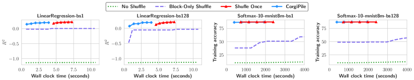
Figure 18: The end-to-end time of linear and softmax regression in PostgreSQL, for clustered datasets on SSD.

Apart from LR/SVM on binary-class datasets, users may also want to train ML models on continuous and multi-class datasets in DB. Thus, we further implement linear regression for training continuous dataset and softmax regression (i.e., multinomial logistic regression) for multi-class datasets, based on our in-DB operators in PostgreSQL. Figure 18 shows the end-to-end execution time of linear regression for continuous YearPredictionMSD dataset [3] and softmax regression for 10-class mini8m dataset [3], with different batch sizes on SSD. Our CorgiPile again achieves similar convergence rate and accuracy (i.e., coefficient of determination $R^{2}$ for linear regression) with the best Shuffle Once, but 1.6-2.1$\times$ faster than it to converge.

7.4.3 Beyond label-clustered datasets

We conduct additional experiments using LR and SVM on all the binary-class datasets ordered by features instead of the labels. For low-dimensional higgs and susy, we sort each feature of them and report the statistics of the converged accuracy in Figure 19. For the other three high-dimensional datasets, we select 9 features such that 3/3/3 of them have the highest/lowest/median correlations with the labels.

Figure 19 shows that No Shuffle again leads to lower accuracy than Shuffle Once. Only for yfcc with image-extracted features and epsilon (with unknown features [1]), the accuracy gap is limited. In contrast, CorgiPile achieves similar converged accuracy to Shuffle Once on all the datasets. This implies simply scanning does not work on the datasets clustered by labels or by features.

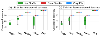
Figure 19: The converged accuracy of LR and SVM on the datasets ordered by features instead of the label.

8 Related Work

Stochastic gradient descent (SGD)

SGD is broadly used in machine learning to solve large-scale optimization problems [28]. It admits the convergence rate $O(1/T)$ for strongly convex objectives, and $O(1/\sqrt{T})$ for the general convex case [61, 38], where $T$ refers to the number of iterations. For non-convex optimization problems, an ergodic convergence rate $O(1/\sqrt{T})$ is proved in [38], and the convergence rate is $O(1/T)$ (e.g., [42]) under the Polyak-Łojasiewicz condition [65]. In the analysis of the above cases, the common assumption is that data is sampled uniformly and independently with replacement in each epoch. We call SGD methods based on this assumption as vanilla SGD.

Data shuffling strategies for SGD

In practice, random-shuffle SGD is a more practical and efficient way of implementing SGD [29]. In each epoch, the data is reshuffled and iterated one by one without replacement. Empirically, it can also be observed that random-shuffle SGD converges much faster than vanilla SGD [27, 40, 42]. In Section 3, we empirically studied the state-of-the-art data shuffling strategies for SGD, including Epoch Shuffle, No Shuffle, Shuffle Once, Sliding-Window Shuffle [18] and MRS Shuffle [37]. Our empirical study shows that Shuffle Once achieves good convergence rate but suffers from low performance, whereas other strategies suffer from low accuracy when running on top of clustered data.

In-DB ML

Previous work [80, 44, 37, 70, 53, 63, 32, 67, 50, 56, 45, 57, 78, 48, 58, 15] has intensively discussed how to implement ML models on relational data, such as linear models [70, 53, 63], linear algebra [32, 56, 57], factorization models [67], neural networks [45, 57, 78] and other statistical learning models [50], using Batch Gradient Descent (BGD) or SGD, over join or self-defined matrix/tensors, etc. The most common way of integrating ML algorithm into RDBMS is to use User-Defined Aggregate Functions (UDA). The representative in-DB ML tools are Apache MADlib [44, 5] and Bismarck [37], which use PostgreSQL’s UDAs to implement SGD, and leverage SQL LOOP (Bismarck) or Python driver (MADlib) to implement iterations. Recently, DB4ML [46] proposes another approach called iterative transactions to implement iterative SGD/graph algorithm in DB. However, it still uses/assumes the Shuffle Once strategy as that of Bismarck/MADlib. Since the source code of DB4ML has not been released yet, we only compare with MADlib and Bismarck.

Scalable ML for distributed data systems

In recent years, there has been active research on integrating ML models into distributed database systems to enable scalable ML, such as MADlib on Greenplum [20], Vertica-ML [36], Google’s BigQuery ML [9], Microsoft SQL Server ML Services [14], etc. Another trend is to leverage big data systems to build scalable ML models based on different architectures, e.g., MPI [33, 49], MapReduce [59, 83, 31], Parameter Server [35, 75, 47] and decentralization [54, 73]. Recent work also started discussing how to integrate deep learning into databases [82, 62]. Our CorgiPile is a general data shuffling strategy for SGD and has been integrated into PyTorch and PostgreSQL. We believe that CorgiPile can be potentially integrated into more above distributed data systems.

9 Conclusion

We have presented CorgiPile, a simple but novel data shuffling strategy for efficient SGD computation on top of block-addressable secondary storage systems such as HDD and SSD. CorgiPile adopts a two-level (i.e., block-level and tuple-level) hierarchical shuffle mechanism that avoids the computation and storage overhead of full data shuffling while retaining similar convergence rates of SGD as if a full data shuffle were performed. We provide a rigorous theoretical analysis on the convergence behavior of CorgiPile and further integrate it into both PyTorch and PostgreSQL. Experimental evaluations demonstrate both statistical and hardware efficiency of CorgiPile when compared to state-of-the-art deep learning system as well as the in-DB ML systems on top of PostgreSQL.

Appendix A I/O performance on HDD and SSD

We have performed an I/O test on the HDD and SSD with different block sizes. As illustrated in Figure 20, on most modern devices, randomly accessing small data tuple can be significantly slower than sequentially scanning data tuples (shown as the dash lines). However, as the block size grows to a reasonable size (e.g., 10MB in this case), the performance of randomly accessing blocks matches the performance of sequential scan. In other words, random access block-wise can match the speed of a full shuffle while the order of data tuples stay untouched.

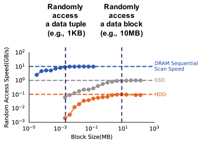
Figure 20: Random Access Performance vs. Block Size.

Appendix B Resource Usage in PostgreSQL

CorgiPile has higher CPU consumption than No Shuffle and Shuffle Once, because it performs data loading and the SGD computation concurrently using two hyper-threads on the same physical CPU core. For example, for criteo on HDD, the maximum CPU usage of our CorgiPile is 115%, where the SGD-computation thread runs with 100% CPU usage and the data-loading thread runs with 15% CPU usage. MRS Shuffle, Sliding-Window Shuffle, and CorgiPile have higher memory consumption than No Shuffle, since they need to allocate buffers in memory. Shuffle Once not only requires additional memory for data shuffling, but also requires 2$\times$ disk space to store the shuffled data.

The Proof of the Theorems

Appendix A Preliminaries

Before presenting our theoretical analysis, we first show some preliminary definitions and lemmas which is important to our proofs.

Lemma 1.

Suppose $f:\mathbb{R}^{d}\mapsto\mathbb{R}$ is a $\mu$-strongly convex function. Then $\forall\mathbf{x},\mathbf{y}\in\mathbb{R}^{d}$, there is

$$F(\mathbf{x})-F(\mathbf{y})\geq\langle\nabla F(\mathbf{x}),\mathbf{y}-\mathbf{x}\rangle+\frac{\mu}{2}\|\mathbf{x}-\mathbf{y}\|^{2}$$

Lemma 2.

Suppose $f(\mathbf{x})$ is an $L$-smooth convex function. Then $\forall\mathbf{x},\mathbf{x}^{*}\in\mathbb{R}^{d}$ where $\mathbf{x}^{*}$ is one global optimum of $f(\mathbf{x})$, there is

$$\|\nabla f(\mathbf{x})\|_{2}^{2}\leq 2L\left(f(\mathbf{x})-f(\mathbf{x}^{*})\right)$$

Fact 1.

Suppose $f:\mathbb{R}^{d}\mapsto\mathbb{R}$ is twice continuously differentiable. $\nabla f(\mathbf{x})\in\mathbb{R}^{d}$ and $H(\mathbf{x})\in\mathbb{R}^{d\times d}$ denote its derivative and Hessian at the point $\mathbf{x}\in\mathbb{R}^{d}$. Then we have, $\forall\mathbf{y},\mathbf{z}\in\mathbb{R}^{d}$,

$$\nabla f(\mathbf{z})-\nabla f(\mathbf{y})=\int_{0}^{\|\mathbf{z}-\mathbf{y}\|}H\left(\mathbf{y}+\frac{\mathbf{z}-\mathbf{y}}{\|\mathbf{z}-\mathbf{y}\|}t\right)\frac{\mathbf{z}-\mathbf{y}}{\|\mathbf{z}-\mathbf{y}\|}\ \ \mathrm{d}t.$$

For simplification, we further define

$$\int_{\mathbf{y}}^{\mathbf{z}}H(\mathbf{x})\mathrm{d}\mathbf{x}:=\int_{0}^{\|\mathbf{z}-\mathbf{y}\|}H\left(\mathbf{y}+\frac{\mathbf{z}-\mathbf{y}}{\|\mathbf{z}-\mathbf{y}\|}t\right)\frac{\mathbf{z}-\mathbf{y}}{\|\mathbf{z}-\mathbf{y}\|}\ \ \mathrm{d}t.$$

which thus lead to $\nabla f(\mathbf{z})-\nabla f(\mathbf{y})=\int_{\mathbf{y}}^{\mathbf{z}}H(\mathbf{x})\mathrm{d}\mathbf{x}$.

Lemma 3.

Suppose there are two non-negative sequences $\{a_{s}\}_{s=0}^{+\infty}$, $\{b_{s}\}_{s=0}^{+\infty}$ satisfying

$$A_{0}\eta_{s}a_{s}\leq(1-\mu A_{1}\eta_{s})b_{s}-b_{s+1}+A_{2}\eta_{s}^{2}+A_{3}\eta_{s}^{3}+A_{4}\eta_{s}^{4}$$

where $\eta_{s}=\frac{3}{A_{1}\mu(s+a)}$ with $a\geq 1$, $\mu>0,A_{0}>0,A_{1}>0,A_{2}>0,A_{3}>0,A_{4}>0$ are constants. Then we have, for $S\geq 0$,

$$\frac{\sum_{s=1}^{S}w_{s}a_{s}}{\sum_{s=1}^{S}w_{s}}\leq\frac{4A_{1}\mu a^{4}b_{1}}{3A_{0}S^{4}}+\frac{12A_{2}}{A_{0}A_{1}\mu}\frac{\sum_{s=1}^{S}(s+a)^{2}}{S^{4}}+\frac{36A_{3}}{A_{0}A_{1}^{2}\mu^{2}}\frac{\sum_{s=1}^{S}(s+a)}{S^{4}}+\frac{108A_{4}}{A_{0}A_{1}^{3}\mu^{3}}\frac{1}{S^{3}}$$

where we let $w_{s}=(s+a)^{3}$.

Proof.

$$\frac{1-\mu A_{1}\eta_{s}}{\eta_{s}}w_{s}=\left(\frac{1}{\eta_{s}}-\mu A_{1}\right)w_{s}=\frac{A_{1}\mu(s+a-3)(t+a)^{3}}{3}\leq\frac{w_{s-1}}{\eta_{s-1}}=\frac{A_{1}\mu(t+a-1)^{4}}{3}$$

where the inequality can be easily verified with the condition $a\geq 1$.

Thus we have

$$A_{0}w_{s}a_{s}\leq \frac{1-\mu A_{1}\eta_{s}}{\eta_{s}}w_{s}b_{s}-\frac{w_{s}}{\eta_{s}}b_{s+1}+A_{2}w_{s}\eta_{s}+A_{3}w_{s}\eta_{s}^{2}+A_{4}\eta_{s}^{3}w_{s}$$

$$\leq \frac{w_{s-1}}{\eta_{s-1}}b_{s}-\frac{w_{s}}{\eta_{s}}b_{s+1}+A_{2}w_{s}\eta_{s}+A_{3}w_{s}\eta_{s}^{2}+A_{4}\eta_{s}^{3}w_{s}$$

Taking summation on both sides of the above inequality, we have

$$A_{0}\sum_{s=1}^{S}w_{s}a_{s}\leq \frac{w_{0}}{\eta_{0}}b_{1}+A_{2}\sum_{s=1}^{S}w_{s}\eta_{s}+A_{3}\sum_{s=1}^{S}w_{s}\eta_{s}^{2}+A_{4}\eta_{s}^{3}w_{s}$$

$$\leq \frac{w_{0}}{\eta_{0}}b_{1}+\frac{3A_{2}}{A_{1}\mu}\sum_{s=1}^{S}(s+a)^{2}+\frac{9A_{3}}{A_{1}^{2}\mu^{2}}\sum_{s=1}^{S}(s+a)+\frac{27A_{4}}{A_{1}^{3}\mu^{3}}S$$

On the other hand, we also see that $\sum_{s=1}^{S}w_{s}=\sum_{s=1}^{S}(s+a)^{3}\geq\sum_{s=1}^{S}s^{3}\geq\frac{S^{4}}{4}$. Dividing both sides by $\sum_{s=1}^{S}w_{s}$, we can obtain

$$\frac{\sum_{s=1}^{S}w_{s}a_{s}}{\sum_{s=1}^{S}w_{s}}\leq\frac{4A_{1}\mu a^{4}b_{1}}{3A_{0}S^{4}}+\frac{12A_{2}}{A_{0}A_{1}\mu}\frac{\sum_{s=1}^{S}(s+a)^{2}}{S^{4}}+\frac{36A_{3}}{A_{0}A_{1}^{2}\mu^{2}}\frac{\sum_{s=1}^{S}(s+a)}{S^{4}}+\frac{108A_{4}}{A_{0}A_{1}^{3}\mu^{3}}\frac{1}{S^{3}}$$

∎

The main structure of our proof is based on the work of [42], which tries to theoretically analyze the full shuffle SGD. However, our proofs below are not a trivial extension of the existing work. The key ingredients in our proofs employing some new techniques are the improvement of estimating the upper bounds of $\mathcal{I}_{1}$ and $\mathcal{I}_{4}$ in the proof of Theorem 1 and the related parts in the proofs of other theorems.

Appendix B Proofs for CorgiPile

Recall that at the $k$-th iteration in the $s$-th epoch, our parameter updating rule can be formulated as follows,

$$\mathbf{x}^{s}_{k}=\mathbf{x}^{s}_{k-1}-\eta_{s}\nabla f_{\psi_{s}(k)}\left(\mathbf{x}^{s}_{k-1}\right),$$ (3)

where $\eta_{s}$ is the learning rate for the $s$-th epoch.

If we recursively apply this updating rule (3), we have that, at the $k$-th iteration in the $s$-th epoch,

$$\mathbf{x}^{s}_{k}=\mathbf{x}^{s}_{0}-\eta_{s}\sum_{k^{\prime}=1}^{k}\nabla f_{\psi_{s}(k^{\prime})}\left(\mathbf{x}^{s}_{k^{\prime}-1}\right),$$ (4)

After the updates of one epoch, i.e., after $bn$ steps in the $s$-th epoch, applying (4), we have

$$\mathbf{x}^{s+1}_{0}=\mathbf{x}^{s}_{0}-\eta_{s}\sum_{k=1}^{bn}\nabla f_{\psi_{s}(k)}\left(\mathbf{x}^{s}_{k-1}\right),$$ (5)

where we use the fact that

$$\mathbf{x}^{s+1}_{0}=\mathbf{x}^{s}_{bn}.$$

B.1 Proof of Theorem 1

Based on the updating rules above, our proof starts from the following formulation,

$$\mathbb{E}\|\mathbf{x}_{0}^{s+1}-\mathbf{x}^{*}\|^{2}$$

$$= \mathbb{E}\|\mathbf{x}_{0}^{s}-\eta_{s}\sum_{k=1}^{bn}\nabla f_{\psi_{s}(k)}(\mathbf{x}^{s}_{k-1})-\mathbf{x}^{*}\|^{2}$$

$$= \mathbb{E}\|\mathbf{x}_{0}^{s}-\mathbf{x}^{*}\|^{2}-2\eta_{s}\mathbb{E}\left\langle\mathbf{x}_{0}^{s}-\mathbf{x}^{*},\sum_{k=1}^{bn}\nabla f_{\psi_{s}(k)}(\mathbf{x}^{s}_{k-1})\right\rangle+\eta_{s}^{2}\mathbb{E}\left\|\sum_{k=1}^{bn}\nabla f_{\psi_{s}(k)}(\mathbf{x}^{s}_{k-1})\right\|^{2}$$

$$\leq \mathbb{E}\|\mathbf{x}_{0}^{s}-\mathbf{x}^{*}\|^{2}-2\eta_{s}\mathbb{E}\left\langle\mathbf{x}_{0}^{s}-\mathbf{x}^{*},\sum_{k=1}^{bn}[\nabla f_{\psi_{s}(k)}(\mathbf{x}^{s}_{k-1})-\nabla f_{\psi_{s}(k)}(\mathbf{x}^{s}_{0})]\right\rangle$$

$$-2\eta_{s}\mathbb{E}\left\langle\mathbf{x}_{0}^{s}-\mathbf{x}^{*},\sum_{k=1}^{bn}\nabla f_{\psi_{s}(k)}(\mathbf{x}^{s}_{0})\right\rangle+2\eta_{s}^{2}\mathbb{E}\left\|\sum_{k=1}^{bn}[\nabla f_{\psi_{s}(k)}(\mathbf{x}^{s}_{k-1})-\nabla f_{\psi_{s}(k)}(\mathbf{x}^{s}_{0})]\right\|^{2}$$

$$+2\eta_{s}^{2}\mathbb{E}\left\|\sum_{k=1}^{bn}\nabla f_{\psi_{s}(k)}(\mathbf{x}^{s}_{0})\right\|^{2}$$

$$= \mathbb{E}\|\mathbf{x}_{0}^{s}-\mathbf{x}^{*}\|^{2}\underbrace{-2\eta_{s}\mathbb{E}\left\langle\mathbf{x}_{0}^{s}-\mathbf{x}^{*},\sum_{k=1}^{bn}[\nabla f_{\psi_{s}(k)}(\mathbf{x}^{s}_{k-1})-\nabla f_{\psi_{s}(k)}(\mathbf{x}^{s}_{0})]\right\rangle}_{\mathcal{I}_{1}}$$

$$\underbrace{-2\eta_{s}\mathbb{E}\left\langle\mathbf{x}_{0}^{s}-\mathbf{x}^{*},\sum_{k=1}^{bn}\nabla f_{\psi_{s}(k)}(\mathbf{x}^{s}_{0})\right\rangle}_{\mathcal{I}_{2}}+\underbrace{2\eta_{s}^{2}\mathbb{E}\left\|\sum_{k=1}^{bn}[\nabla f_{\psi_{s}(k)}(\mathbf{x}^{s}_{k-1})-\nabla f_{\psi_{s}(k)}(\mathbf{x}^{s}_{0})]\right\|^{2}}_{\mathcal{I}_{3}}$$ (6)

$$+\underbrace{2\eta_{s}^{2}\mathbb{E}\left\|\sum_{k=1}^{bn}\nabla f_{\psi_{s}(k)}(\mathbf{x}^{s}_{0})-\mathbb{E}\sum_{k=1}^{bn}\nabla f_{\psi_{s}(k)}(\mathbf{x}^{s}_{0})\right\|^{2}}_{\mathcal{I}_{4}}+\underbrace{2\eta_{s}^{2}\left\|\mathbb{E}\sum_{k=1}^{bn}\nabla f_{\psi_{s}(k)}(\mathbf{x}^{s}_{0})\right\|^{2}}_{\mathcal{I}_{5}}$$

where the last equality uses the fact that $\mathbb{E}\|X-\mathbb{E}[X]\|^{2}=\mathbb{E}\|X\|^{2}-\|\mathbb{E}[X]\|^{2}$.

To prove the upper bound of (6), we need to bound $\mathcal{I}_{1}$, $\mathcal{I}_{2}$, $\mathcal{I}_{3}$, $\mathcal{I}_{4}$ and $\mathcal{I}_{5}$ respectively.

Bound of $\mathcal{I}_{3}$

For $\mathcal{I}_{3}$, we have that

$$\left\|\sum_{k=1}^{bn}[\nabla f_{\psi_{s}(k)}(\mathbf{x}^{s}_{k-1})-\nabla f_{\psi_{s}(k)}(\mathbf{x}^{s}_{0})]\right\|^{2}$$

$$\leq bn\sum_{k=1}^{bn}\left\|\nabla f_{\psi_{s}(k)}(\mathbf{x}^{s}_{k-1})-\nabla f_{\psi_{s}(k)}(\mathbf{x}^{s}_{0})\right\|^{2}$$

$$\leq bn\sum_{k=1}^{bn}L^{2}\left\|\mathbf{x}^{s}_{k-1}-\mathbf{x}^{s}_{0}\right\|^{2}$$

$$\leq bn\sum_{k=1}^{bn}L^{2}\left\|\eta_{s}\sum_{k^{\prime}=1}^{k-1}\nabla f_{\psi_{s}(k^{\prime})}(\mathbf{x}^{s}_{k^{\prime}-1})\right\|^{2}$$

$$\leq bn\sum_{k=1}^{bn}\eta_{s}^{2}L^{2}(k-1)\sum_{k^{\prime}=1}^{k-1}\left\|\nabla f_{\psi_{s}(k^{\prime})}(\mathbf{x}^{s}_{k^{\prime}-1})\right\|^{2}$$

$$\leq \eta_{s}^{2}L^{2}G^{2}bn\sum_{k=1}^{bn}(k-1)^{2}\leq\frac{1}{3}\eta_{s}^{2}L^{2}G^{2}(bn)^{4}$$

where the first and the fourth inequalities uses the fact that $\|\sum_{k=1}^{bn}\mathbf{a}_{k}\|^{2}\leq bn\sum_{k=1}^{bn}\|\mathbf{a}_{k}\|^{2}$, the second inequality holds due to the Lipschitz continuity of the gradient, the third inequality is due to $\mathbf{x}^{s}_{k-1}=\mathbf{x}^{s}_{0}-\eta_{s}\sum_{k^{\prime}=1}^{k-1}\nabla f_{\psi_{s}(k^{\prime})}(\mathbf{x}^{s}_{k^{\prime}-1})$ and the last inequality is due to $\sum_{i=1}^{n}i^{2}=\frac{n(n+1)(2n+1)}{6}$ and the boundedness of the gradient.

Therefore, we have

$$\mathcal{I}_{3}=2\eta_{s}^{2}\mathbb{E}\left\|\sum_{k=1}^{bn}[\nabla f_{\psi_{s}(k)}(\mathbf{x}^{s}_{k-1})-\nabla f_{\psi_{s}(k)}(\mathbf{x}^{s}_{0})]\right\|^{2}\leq\frac{2}{3}\eta_{s}^{4}L^{2}G^{2}K^{4}$$ (7)

Bounds of $\mathcal{I}_{2}$ and $\mathcal{I}_{5}$

For $\mathcal{I}_{2}$ and $\mathcal{I}_{5}$, the key is to know the form of $\mathbb{E}\sum_{k=1}^{bn}\nabla f_{\psi_{s}(k)}(\mathbf{x}^{s}_{0})$.

$$\mathbb{E}\sum_{k=1}^{bn}\nabla f_{\psi_{s}(k)}(\mathbf{x}^{s}_{0})= \mathbb{E}\sum_{B_{l}\in\mathcal{B}_{s}}\sum_{i\in B_{l}}\nabla f_{i}(\mathbf{x}_{0}^{s}),$$

where this equality holds since the random shuffling $\psi_{s}$ does not affect the summation in the LHS formula.

Furthermore, we use indicator random variables to get the value of $\mathbb{E}\sum_{B_{l}\in\mathcal{B}_{s}}\sum_{i\in B_{l}}\nabla f_{i}(\mathbf{x}_{0}^{s})$. Let $\mathbb{I}_{B_{l}\in\mathcal{B}_{s}}$ be the random variable to indicate whether the block $B_{l}$ is in $\mathcal{B}_{s}$ or not. Therefore, we have

$$\mathbb{I}_{B_{l}\in\mathcal{B}_{s}}=\begin{cases}1,&\text{ if }B_{l}\in\mathcal{B}_{s}\\ 0,&\text{ if }B_{l}\notin\mathcal{B}_{s}\end{cases},$$

and

$$\mathbb{P}(\mathbb{I}_{B_{l}\in\mathcal{B}_{s}}=1)=\mathbb{P}(B_{l}\in\mathcal{B}_{s})=\frac{\binom{1}{1}\binom{N-1}{n-1}}{\binom{N}{n}}=\frac{n}{N}$$

such that $\mathbb{E}[\mathbb{I}_{B_{l}\in\mathcal{B}_{s}}]=\frac{n}{N}$.

Thus, we can obtain

$$\mathbb{E}\sum_{B_{l}\in\mathcal{B}_{s}}\sum_{i\in B_{l}}\nabla f_{i}(\mathbf{x}_{0}^{s})=\mathbb{E}\sum_{l=1}^{N}\mathbb{I}_{B_{l}\in\mathcal{B}_{s}}\left(\sum_{i\in B_{l}}\nabla f_{i}(\mathbf{x}_{0}^{s})\right)=\frac{n}{N}\sum_{l=1}^{N}\sum_{i\in B_{l}}\nabla f_{i}(\mathbf{x}_{0}^{s})=\frac{n}{N}m\nabla F(\mathbf{x}^{s}_{0}).$$

Therefore, we get the values of $\mathcal{I}_{2}$ and $\mathcal{I}_{5}$

$$\mathcal{I}_{2}=-2\eta_{s}\mathbb{E}\left\langle\mathbf{x}_{0}^{s}-\mathbf{x}^{*},\sum_{k=1}^{bn}\nabla f_{\psi_{s}(k)}(\mathbf{x}^{s}_{0})\right\rangle=-2\eta_{s}\frac{n}{N}m\mathbb{E}\left\langle\mathbf{x}_{0}^{s}-\mathbf{x}^{*},\nabla F(\mathbf{x}_{0}^{s})\right\rangle$$ (8)

$$\mathcal{I}_{5}=2\eta_{s}^{2}\left\|\mathbb{E}\sum_{k=1}^{bn}\nabla f_{\psi_{s}(k)}(\mathbf{x}^{s}_{0})\right\|^{2}=2\eta_{s}^{2}\frac{n^{2}}{N^{2}}m^{2}\left\|\nabla F(\mathbf{x}^{s}_{0})\right\|^{2}$$ (9)

Bound of $\mathcal{I}_{4}$

Next, we will show the variance of sampling the $n$ blocks out of $N$ without replacement. We still use the indicator variables defined above.

The upper bound of $\mathcal{I}_{4}$ determines the $\frac{1}{T}$ term and the $\frac{N-n}{N-1}$ factor existing in the convergence rate, which shows how the leading term $\frac{N-n}{N-1}\frac{1}{T}$ varying with the number of sampled blocks $n$.

Note that for any $l^{\prime}\neq l^{\prime\prime}$, we have

$$\mathbb{P}(\mathbb{I}_{B_{l^{\prime}}\in\mathcal{B}_{s}}=1,\mathbb{I}_{B_{l^{\prime\prime}}\in\mathcal{B}_{s}}=1)=\mathbb{P}(B_{l^{\prime}}\in\mathcal{B}_{s}\wedge B_{l^{\prime\prime}}\in\mathcal{B}_{s})=\frac{\binom{2}{2}\binom{N-2}{n-2}}{\binom{N}{n}}=\frac{n(n-1)}{N(N-1)}$$

Therefore, $\mathbb{E}[\mathbb{I}_{B_{l^{\prime}}\in\mathcal{B}_{s}}\cdot\mathbb{I}_{B_{l^{\prime\prime}}\in\mathcal{B}_{s}}]=\frac{n(n-1)}{N(N-1)}$.

$$\mathbb{E}\left\|\sum_{k=1}^{bn}\nabla f_{\psi_{s}(k)}(\mathbf{x}^{s}_{0})-\mathbb{E}\sum_{k=1}^{bn}\nabla f_{\psi_{s}(k)}(\mathbf{x}^{s}_{0})\right\|^{2}$$

$$= \mathbb{E}\left\|\sum_{l=1}^{N}\mathbb{I}_{B_{l}\in\mathcal{B}_{s}}\left(\sum_{i\in B_{l}}\nabla f_{i}(\mathbf{x}_{0}^{s})\right)-\mathbb{E}\sum_{l=1}^{N}\mathbb{I}_{B_{l}\in\mathcal{B}_{s}}\left(\sum_{i\in B_{l}}\nabla f_{i}(\mathbf{x}_{0}^{s})\right)\right\|^{2}$$

$$= \mathbb{E}\left\|\sum_{l=1}^{N}\mathbb{I}_{B_{l}\in\mathcal{B}_{s}}\left(\sum_{i\in B_{l}}\nabla f_{i}(\mathbf{x}_{0}^{s})\right)\right\|^{2}-\left\|\frac{n}{N}\sum_{l=1}^{N}\left(\sum_{i\in B_{l}}\nabla f_{i}(\mathbf{x}_{0}^{s})\right)\right\|^{2}$$

$$= \mathbb{E}\sum_{l=1}^{N}\mathbb{I}_{B_{l}\in\mathcal{B}_{s}}\cdot\mathbb{I}_{B_{l}\in\mathcal{B}_{s}}\left\|\sum_{i\in B_{l}}\nabla f_{i}(\mathbf{x}_{0}^{s})\right\|^{2}+\mathbb{E}\sum_{l^{\prime}\neq l^{\prime\prime}}\mathbb{I}_{B_{l^{\prime}}\in\mathcal{B}_{s}}\cdot\mathbb{I}_{B_{l^{\prime\prime}}\in\mathcal{B}_{s}}\left\langle\sum_{i\in B_{l^{\prime}}}\nabla f_{i}(\mathbf{x}_{0}^{s}),\sum_{i\in B_{l^{\prime\prime}}}\nabla f_{i}(\mathbf{x}_{0}^{s})\right\rangle$$

$$-\frac{n^{2}}{N^{2}}\sum_{l=1}^{N}\left\|\sum_{i\in B_{l}}\nabla f_{i}(\mathbf{x}_{0}^{s})\right\|^{2}-\frac{n^{2}}{N^{2}}\sum_{l^{\prime}\neq l^{\prime\prime}}^{N}\left\langle\sum_{i\in B_{l^{\prime}}}\nabla f_{i}(\mathbf{x}_{0}^{s}),\sum_{i\in B_{l^{\prime\prime}}}\nabla f_{i}(\mathbf{x}_{0}^{s})\right\rangle$$

$$= \mathbb{E}\sum_{l=1}^{N}\mathbb{I}_{B_{l}\in\mathcal{B}_{s}}\cdot\mathbb{I}_{B_{l}\in\mathcal{B}_{s}}\left\|\sum_{i\in B_{l}}\nabla f_{i}(\mathbf{x}_{0}^{s})\right\|^{2}+\mathbb{E}\sum_{l^{\prime}\neq l^{\prime\prime}}\mathbb{I}_{B_{l^{\prime}}\in\mathcal{B}_{s}}\cdot\mathbb{I}_{B_{l^{\prime\prime}}\in\mathcal{B}_{s}}\left\langle\sum_{i\in B_{l^{\prime}}}\nabla f_{i}(\mathbf{x}_{0}^{s}),\sum_{i\in B_{l^{\prime\prime}}}\nabla f_{i}(\mathbf{x}_{0}^{s})\right\rangle$$

$$-\frac{n^{2}}{N^{2}}\sum_{l=1}^{N}\left\|\sum_{i\in B_{l}}\nabla f_{i}(\mathbf{x}_{0}^{s})\right\|^{2}-\frac{n^{2}}{N^{2}}\sum_{l^{\prime}\neq l^{\prime\prime}}^{N}\left\langle\sum_{i\in B_{l^{\prime}}}\nabla f_{i}(\mathbf{x}_{0}^{s}),\sum_{i\in B_{l^{\prime\prime}}}\nabla f_{i}(\mathbf{x}_{0}^{s})\right\rangle$$

$$= \left(\frac{n}{N}-\frac{n^{2}}{N^{2}}\right)\sum_{l=1}^{N}\left\|\sum_{i\in B_{l}}\nabla f_{i}(\mathbf{x}_{0}^{s})\right\|^{2}+\left(\frac{n(n-1)}{N(N-1)}-\frac{n^{2}}{N^{2}}\right)\sum_{l^{\prime}\neq l^{\prime\prime}}\left\langle\sum_{i\in B_{l^{\prime}}}\nabla f_{i}(\mathbf{x}_{0}^{s}),\sum_{i\in B_{l^{\prime\prime}}}\nabla f_{i}(\mathbf{x}_{0}^{s})\right\rangle$$

where the last equality is due to $\mathbb{E}[\mathbb{I}_{B_{l}\in\mathcal{B}_{s}}\cdot\mathbb{I}_{B_{l}\in\mathcal{B}_{s}}]=\mathbb{E}[\mathbb{I}_{B_{l}\in\mathcal{B}_{s}}]=\frac{n}{N}$ and $\mathbb{E}[\mathbb{I}_{B_{l^{\prime}}\in\mathcal{B}_{s}}\cdot\mathbb{I}_{B_{l^{\prime\prime}}\in\mathcal{B}_{s}}]=\frac{n(n-1)}{N(N-1)}$, and the second equality is due to $\mathbb{E}\|X-\mathbb{E}X\|^{2}=\mathbb{E}\|X\|^{2}-\|\mathbb{E}X\|^{2}$.

On the other hand, we have

$$\mathbb{E}_{l}\left\|\sum_{i\in B_{l}}\nabla f_{i}(\mathbf{x}_{0}^{s})-b\nabla F(\mathbf{x}_{0}^{s})\right\|^{2}$$

$$= \mathbb{E}_{l}\left\|\sum_{i\in B_{l}}\nabla f_{i}(\mathbf{x}_{0}^{s})-\mathbb{E}_{l}\sum_{i\in B_{l}}\nabla f_{i}(\mathbf{x}_{0}^{s})\right\|^{2}$$

$$= \mathbb{E}_{l}\left\|\sum_{i\in B_{l}}\nabla f_{i}(\mathbf{x}_{0}^{s})-\frac{1}{N}\sum_{l=1}^{N}\sum_{i\in B_{l}}\nabla f_{i}(\mathbf{x}_{0}^{s})\right\|^{2}$$

$$= \mathbb{E}_{l}\left\|\sum_{i\in B_{l}}\nabla f_{i}(\mathbf{x}_{0}^{s})\right\|^{2}-\frac{1}{N^{2}}\left\|\sum_{l=1}^{N}\sum_{i\in B_{l}}\nabla f_{i}(\mathbf{x}_{0}^{s})\right\|^{2}$$

$$= \frac{1}{N}\sum_{l=1}^{N}\left\|\sum_{i\in B_{l}}\nabla f_{i}(\mathbf{x}_{0}^{s})\right\|^{2}-\frac{1}{N^{2}}\sum_{l=1}^{N}\left\|\sum_{i\in B_{l}}\nabla f_{i}(\mathbf{x}_{0}^{s})\right\|^{2}-\frac{1}{N^{2}}\sum_{l^{\prime}\neq l^{\prime\prime}}\left\langle\sum_{i\in B_{l^{\prime}}}\nabla f_{i}(\mathbf{x}_{0}^{s}),\sum_{i\in B_{l^{\prime\prime}}}\nabla f_{i}(\mathbf{x}_{0}^{s})\right\rangle$$

$$= \left(\frac{1}{N}-\frac{1}{N^{2}}\right)\sum_{l=1}^{N}\left\|\sum_{i\in B_{l}}\nabla f_{i}(\mathbf{x}_{0}^{s})\right\|^{2}-\frac{1}{N^{2}}\sum_{l^{\prime}\neq l^{\prime\prime}}\left\langle\sum_{i\in B_{l^{\prime}}}\nabla f_{i}(\mathbf{x}_{0}^{s}),\sum_{i\in B_{l^{\prime\prime}}}\nabla f_{i}(\mathbf{x}_{0}^{s})\right\rangle.$$

By comparing the RHS of the above two equations, we can observe that

$$\mathbb{E}\left\|\sum_{k=1}^{bn}\nabla f_{\psi_{s}(k)}(\mathbf{x}^{s}_{0})-\mathbb{E}\sum_{k=1}^{bn}\nabla f_{\psi_{s}(k)}(\mathbf{x}^{s}_{0})\right\|^{2}=\frac{n(N-n)}{N-1}\mathbb{E}_{\xi^{\prime}}\left\|\sum_{i\in B_{\xi^{\prime}}}\nabla f_{i}(\mathbf{x}_{0}^{s})-b\nabla F(\mathbf{x}_{0}^{s})\right\|^{2}.$$

If we further apply our assumption that $\mathbb{E}_{\xi^{\prime}}\left\|\frac{1}{b}\sum_{i\in B_{\xi^{\prime}}}\nabla f_{i}(\mathbf{x}_{0}^{s})-\nabla F(\mathbf{x}_{0}^{s})\right\|^{2}\leq h_{D}\frac{\sigma^{2}}{b}$, then there is

$$\mathcal{I}_{4}=2\eta^{2}_{s}\mathbb{E}\left\|\sum_{k=1}^{bn}\nabla f_{\psi_{s}(k)}(\mathbf{x}^{s}_{0})-\mathbb{E}\sum_{k=1}^{bn}\nabla f_{\psi_{s}(k)}(\mathbf{x}^{s}_{0})\right\|^{2}\leq 2\eta^{2}_{s}\frac{nb(N-n)}{N-1}h_{D}\sigma^{2}$$ (10)

This result shows the connection between the variance of block-wise sampling without replacement and the variance of sampling single data point independently and uniformly.

Bound of $\mathcal{I}_{1}$

The upper bound of $\mathcal{I}_{1}$ is critical to the proof of obtaining a faster rate. Before presenting the upper bound of $\mathcal{I}_{1}$, recall the Fact 1 that

$$\nabla f(\mathbf{z})-\nabla f(\mathbf{y})=\int_{\mathbf{y}}^{\mathbf{z}}H(\mathbf{x})\mathrm{d}\mathbf{x}:=\int_{0}^{\|\mathbf{z}-\mathbf{y}\|}H\left(\mathbf{y}+\frac{\mathbf{z}-\mathbf{y}}{\|\mathbf{z}-\mathbf{y}\|}t\right)\frac{\mathbf{z}-\mathbf{y}}{\|\mathbf{z}-\mathbf{y}\|}\ \ \mathrm{d}t.$$

Now we can show the upper bound of $\mathcal{I}_{1}$ as follows,

$$\mathcal{I}_{1}= -2\eta_{s}\mathbb{E}\left\langle\mathbf{x}_{0}^{s}-\mathbf{x}^{*},\sum_{k=1}^{bn}[\nabla f_{\psi_{s}(k)}(\mathbf{x}^{s}_{k-1})-\nabla f_{\psi_{s}(k)}(\mathbf{x}^{s}_{0})]\right\rangle$$

$$= -2\eta_{s}\mathbb{E}\left\langle\mathbf{x}_{0}^{s}-\mathbf{x}^{*},\sum_{k=1}^{bn}\int_{\mathbf{x}^{s}_{0}}^{\mathbf{x}^{s}_{k-1}}H_{\psi_{s}(k)}(\mathbf{x})\mathrm{d}\mathbf{x}\right\rangle$$

$$= -2\eta_{s}\mathbb{E}\left\langle\mathbf{x}_{0}^{s}-\mathbf{x}^{*},\sum_{k=1}^{bn}\int_{\mathbf{x}^{s}_{0}}^{\mathbf{x}^{s}_{k-1}}H_{\psi_{s}(k)}(\mathbf{x}^{*})\mathrm{d}\mathbf{x}\right\rangle$$

$$-2\eta_{s}\mathbb{E}\left\langle\mathbf{x}_{0}^{s}-\mathbf{x}^{*},\sum_{k=1}^{bn}\int_{\mathbf{x}^{s}_{0}}^{\mathbf{x}^{s}_{k-1}}\left(H_{\psi_{s}(k)}(\mathbf{x})-H_{\psi_{s}(k)}(\mathbf{x}^{*})\right)\mathrm{d}\mathbf{x}\right\rangle$$

$$= -2\eta_{s}\mathbb{E}\left\langle\mathbf{x}_{0}^{s}-\mathbf{x}^{*},\sum_{k=1}^{bn}H_{\psi_{s}(k)}(\mathbf{x}^{*})\left(\mathbf{x}^{s}_{k-1}-\mathbf{x}^{s}_{0}\right)\right\rangle$$

$$-2\eta_{s}\mathbb{E}\left\langle\mathbf{x}_{0}^{s}-\mathbf{x}^{*},\sum_{k=1}^{bn}\int_{\mathbf{x}^{s}_{0}}^{\mathbf{x}^{s}_{k-1}}\left(H_{\psi_{s}(k)}(\mathbf{x})-H_{\psi_{s}(k)}(\mathbf{x}^{*})\right)\mathrm{d}\mathbf{x}\right\rangle$$

$$= 2\eta_{s}^{2}\mathbb{E}\left\langle\mathbf{x}_{0}^{s}-\mathbf{x}^{*},\sum_{k=1}^{bn}H_{\psi_{s}(k)}(\mathbf{x}^{*})\left(\sum_{k^{\prime}=1}^{k-1}\nabla f_{\psi_{s}(k^{\prime})}(\mathbf{x}_{k^{\prime}-1}^{s})\right)\right\rangle$$

$$-2\eta_{s}\mathbb{E}\left\langle\mathbf{x}_{0}^{s}-\mathbf{x}^{*},\sum_{k=1}^{bn}\int_{\mathbf{x}^{s}_{0}}^{\mathbf{x}^{s}_{k-1}}\left(H_{\psi_{s}(k)}(\mathbf{x})-H_{\psi_{s}(k)}(\mathbf{x}^{*})\right)\mathrm{d}\mathbf{x}\right\rangle$$

$$= \underbrace{2\eta_{s}^{2}\mathbb{E}\left\langle\mathbf{x}_{0}^{s}-\mathbf{x}^{*},\sum_{k=1}^{bn}H_{\psi_{s}(k)}(\mathbf{x}^{*})\left(\sum_{k^{\prime}=1}^{k-1}\nabla f_{\psi_{s}(k^{\prime})}(\mathbf{x}_{0}^{s})\right)\right\rangle}_{\mathcal{I}_{11}}$$

$$\underbrace{2\eta_{s}^{2}\mathbb{E}\left\langle\mathbf{x}_{0}^{s}-\mathbf{x}^{*},\sum_{k=1}^{bn}H_{\psi_{s}(k)}(\mathbf{x}^{*})\left(\sum_{k^{\prime}=1}^{k-1}\nabla f_{\psi_{s}(k^{\prime})}(\mathbf{x}_{k^{\prime}-1}^{s})-\nabla f_{\psi_{s}(k^{\prime})}(\mathbf{x}_{0}^{s})\right)\right\rangle}_{\mathcal{I}_{12}}$$

$$\underbrace{-2\eta_{s}\mathbb{E}\left\langle\mathbf{x}_{0}^{s}-\mathbf{x}^{*},\sum_{k=1}^{bn}\int_{\mathbf{x}^{s}_{0}}^{\mathbf{x}^{s}_{k-1}}\left(H_{\psi_{s}(k)}(\mathbf{x})-H_{\psi_{s}(k)}(\mathbf{x}^{*})\right)\mathrm{d}\mathbf{x}\right\rangle}_{\mathcal{I}_{13}}$$

where the second equality holds due to the Fact 1 and the fifth equality holds since we have $\mathbf{x}^{s}_{k-1}=\mathbf{x}^{s}_{0}-\eta_{s}\sum_{k^{\prime}=1}^{k-1}\nabla f_{\psi_{s}(k^{\prime})}(\mathbf{x}^{s}_{k^{\prime}-1})$. Note that $H_{\psi_{s}(k)}(\mathbf{x}^{*})$ is the Hessian of the function $f_{\psi_{s}(k)}(\mathbf{x})$ at the point $\mathbf{x}^{*}$.

In order to obtain the upper bound of $\mathcal{I}_{1}$, we need to bound $\mathcal{I}_{11}$, $\mathcal{I}_{12}$ and $\mathcal{I}_{13}$ separately.

Bound of $\mathcal{I}_{11}$

In $\mathcal{I}_{11}$, we need first compute $\mathbb{E}\sum_{k=1}^{bn}H_{\psi_{s}(k)}(\mathbf{x}^{*})\left(\sum_{k^{\prime}=1}^{k-1}\nabla f_{\psi_{s}(k^{\prime})}(\mathbf{x}_{0}^{s})\right)$, which is the key ingredient for obtaining the $O(\frac{1}{T^{2}})$ term in the convergence rate.

To make our proof more clear, recall the manipulation in our algorithm for obtain $\psi_{s}$:

1. At the $s$-th epoch, random sample $n$ out of the total $N$ blocks without replacement to get a set of sampled blocks $\mathcal{B}_{s}$ with size of $n$. Each block has $b$ data samples.

2. Then, perform random shuffling of the $nb$ data samples and obtain the shuffled index sequence $\psi_{s}$ with $|\psi_{s}|=nb$.

where we define $\mathcal{B}_{s}$ being the set of blocks that are sampled each epoch.

In order to compute the expectation, we use the indicator random variable for a more clear derivation.

Define $\mathbb{I}_{\psi_{s}(k)=i}$ be the indicator random variable showing whether one data sample with index $i$ located in the $k$-th place after the above 2-step manipulation. The event $\psi_{s}(k)=i$ is equivalent to the event that $i\in B_{l}\wedge B_{l}\in\mathcal{B}_{s}\wedge\psi_{s}(k)=i$ where $B_{l}$ is the block that the $i$-th sample lies in.

Thus, we have

$$\mathbb{I}_{\psi_{s}(k)=i}=\begin{cases}1,&\text{ if }\psi_{s}(k)=i\\ 0,&\text{ if }\psi_{s}(k)\neq i\end{cases}$$

and

$$\mathbb{P}(\mathbb{I}_{\psi_{s}(k)=i}=1)=\mathbb{P}(i\in B_{l},B_{l}\in\mathcal{B}_{s},\psi_{s}(k)=i)=\frac{\binom{1}{1}\binom{N-1}{n-1}(bn-1)!}{\binom{N}{n}(bn)!}=\frac{1}{Nb}.$$

Thus, we can observe that

$$H_{\psi_{s}(k)}(\mathbf{x}^{*})=\sum_{i=1}^{m}\mathbb{I}_{\psi_{s}(k)=i}H_{i}(\mathbf{x}^{*})$$

$$\nabla f_{\psi_{s}(k^{\prime})}(\mathbf{x}_{0}^{s})=\sum_{j=1}^{m}\mathbb{I}_{\psi_{s}(k^{\prime})=j}\nabla f_{j}(\mathbf{x}_{0}^{s})$$

Based on the above definition, we are ready to compute the expectation.

$$\mathbb{E}\sum_{k=1}^{bn}H_{\psi_{s}(k)}(\mathbf{x}^{*})\left(\sum_{k^{\prime}=1}^{k-1}\nabla f_{\psi_{s}(k^{\prime})}(\mathbf{x}_{0}^{s})\right)$$

$$= \mathbb{E}\sum_{k=1}^{bn}\sum_{i=1}^{m}\mathbb{I}_{\psi_{s}(k)=i}H_{i}(\mathbf{x}^{*})\left(\sum_{k^{\prime}=1}^{k-1}\sum_{j=1}^{m}\mathbb{I}_{\psi_{s}(k^{\prime})=j}\nabla f_{j}(\mathbf{x}_{0}^{s})\right)$$

$$= \sum_{k=1}^{bn}\sum_{k^{\prime}=1}^{k-1}\sum_{i=1}^{m}\sum_{j=1}^{m}\mathbb{E}\left[\mathbb{I}_{\psi_{s}(k)=i}\cdot\mathbb{I}_{\psi_{s}(k^{\prime})=j}\right]H_{i}(\mathbf{x}^{*})\nabla f_{j}(\mathbf{x}_{0}^{s})$$

$$= \sum_{k=1}^{bn}\sum_{k^{\prime}=1}^{k-1}\sum_{i\neq j}\mathbb{E}\left[\mathbb{I}_{\psi_{s}(k)=i}\cdot\mathbb{I}_{\psi_{s}(k^{\prime})=j}\right]H_{i}(\mathbf{x}^{*})\nabla f_{j}(\mathbf{x}_{0}^{s})$$

where the last equality holds since

$$\mathbb{P}(\mathbb{I}_{\psi_{s}(k)=i}=1,\mathbb{I}_{\psi_{s}(k^{\prime})=i}=1)=0\quad\Rightarrow\quad\mathbb{E}\left[\mathbb{I}_{\psi_{s}(k)=i}\cdot\mathbb{I}_{\psi_{s}(k^{\prime})=i}\right]=0$$

because $k>k^{\prime}$ and one data sample cannot appear in different positions at the same time.

Therefore, for any $k>k^{\prime}$ and $i\neq j$,

1. If $i\in B_{l}$,$j\in B_{l}$, we have

   $$\mathbb{P}(\mathbb{I}_{\psi_{s}(k)=i}=1,\mathbb{I}_{\psi_{s}(k^{\prime})=j}=1)=\frac{\binom{1}{1}\binom{N-1}{n-1}(nb-2)!}{\binom{N}{n}(nb)!}=\frac{1}{Nb(nb-1)}$$

   $$\Rightarrow$$

   $$\mathbb{E}\left[\mathbb{I}_{\psi_{s}(k)=i}\cdot\mathbb{I}_{\psi_{s}(k^{\prime})=j}\right]=\frac{1}{Nb(nb-1)}.$$

   where $\binom{1}{1}$ means $B_{l}$ are chosen ahead, $\binom{N-1}{n-1}$ means $(n-1)$ blocks excluding $B_{l}$ are randomly chosen from $N-1$ blocks excluding $B_{l}$, $\binom{N}{n}$ is the total number of ways of choosing $n$ blocks from $N$ blocks, $(nb-2)!$ is the number of ways of shuffling the data in $n$ blocks expect $i$ and $j$, and $(nb)!$ is the number of ways of shuffling all the data in $n$ blocks.

2. If $i\in B_{l}$,$j\in B_{l}$ and $l\neq l^{\prime}$, we have

   $$\mathbb{P}(\mathbb{I}_{\psi_{s}(k)=i}=1,\mathbb{I}_{\psi_{s}(k^{\prime})=j}=1)=\frac{\binom{2}{2}\binom{N-2}{n-2}(nb-2)!}{\binom{N}{n}(nb)!}=\frac{n-1}{Nb(N-1)(nb-1)}.$$

   $$\Rightarrow$$

   $$\mathbb{E}\left[\mathbb{I}_{\psi_{s}(k)=i}\cdot\mathbb{I}_{\psi_{s}(k^{\prime})=j}\right]=\frac{n-1}{Nb(N-1)(nb-1)}.$$

   where $\binom{2}{2}$ means $B_{l}$ and $B_{l^{\prime}}$ are chosen ahead, $\binom{N-2}{n-2}$ means $(n-2)$ blocks excluding $B_{l}$ and $B_{l^{\prime}}$ are randomly chosen from $N-2$ blocks excluding $B_{l}$ and $B_{l^{\prime}}$, $\binom{N}{n}$ is the total number of ways of choosing $n$ blocks from $N$ blocks, $(nb-2)!$ is the number of ways of shuffling the data in $n$ blocks expect $i$ and $j$, and $(nb)!$ is the number of ways of shuffling all the data in $n$ blocks.

Thus, we have

$$\mathbb{E}\sum_{k=1}^{bn}H_{\psi_{s}(k)}(\mathbf{x}^{*})\left(\sum_{k^{\prime}=1}^{k-1}\nabla f_{\psi_{s}(k^{\prime})}(\mathbf{x}_{0}^{s})\right)$$

$$= \sum_{k=1}^{bn}\sum_{k^{\prime}=1}^{k-1}\sum_{i\neq j}\mathbb{E}\left[\mathbb{I}_{\psi_{s}(k)=i}\cdot\mathbb{I}_{\psi_{s}(k^{\prime})=j}\right]H_{i}(\mathbf{x}^{*})\nabla f_{j}(\mathbf{x}_{0}^{s})$$

$$= \sum_{k=1}^{bn}\sum_{k^{\prime}=1}^{k-1}\Bigg{(}\sum_{l=1}^{N}\sum_{\begin{subarray}{c}i\neq j\\ i,j\in B_{l}\end{subarray}}\mathbb{E}\left[\mathbb{I}_{\psi_{s}(k)=i}\cdot\mathbb{I}_{\psi_{s}(k^{\prime})=j}\right]H_{i}(\mathbf{x}^{*})\nabla f_{j}(\mathbf{x}_{0}^{s})$$

$$+\sum_{l\neq l^{\prime}}\sum_{\begin{subarray}{c}i,j\\ i\in B_{l},j\in B_{l^{\prime}}\end{subarray}}\mathbb{E}\left[\mathbb{I}_{\psi_{s}(k)=i}\cdot\mathbb{I}_{\psi_{s}(k^{\prime})=j}\right]H_{i}(\mathbf{x}^{*})\nabla f_{j}(\mathbf{x}_{0}^{s})\Bigg{)}$$

$$= \frac{nb(nb-1)}{2}\left(\sum_{l=1}^{N}\sum_{\begin{subarray}{c}i\neq j\\ i,j\in B_{l}\end{subarray}}\frac{1}{Nb(nb-1)}H_{i}(\mathbf{x}^{*})\nabla f_{j}(\mathbf{x}_{0}^{s})+\sum_{l\neq l^{\prime}}\sum_{\begin{subarray}{c}i,j\\ i\in B_{l},j\in B_{l^{\prime}}\end{subarray}}\frac{n-1}{Nb(N-1)(nb-1)}H_{i}(\mathbf{x}^{*})\nabla f_{j}(\mathbf{x}_{0}^{s})\right)$$

$$= \sum_{l=1}^{N}\sum_{\begin{subarray}{c}i\neq j\\ i,j\in B_{l}\end{subarray}}\frac{n}{2N}H_{i}(\mathbf{x}^{*})\nabla f_{j}(\mathbf{x}_{0}^{s})+\sum_{l\neq l^{\prime}}\sum_{\begin{subarray}{c}i,j\\ i\in B_{l},j\in B_{l^{\prime}}\end{subarray}}\frac{n(n-1)}{2N(N-1)}H_{i}(\mathbf{x}^{*})\nabla f_{j}(\mathbf{x}_{0}^{s})$$

Plugging in the above result into $\mathcal{I}_{11}$, we can get

$$\mathcal{I}_{11}= 2\eta_{s}^{2}\mathbb{E}\left\langle\mathbf{x}_{0}^{s}-\mathbf{x}^{*},\sum_{l=1}^{N}\sum_{\begin{subarray}{c}i\neq j\\ i,j\in B_{l}\end{subarray}}\frac{n}{2N}H_{i}(\mathbf{x}^{*})\nabla f_{j}(\mathbf{x}_{0}^{s})+\sum_{l\neq l^{\prime}}\sum_{\begin{subarray}{c}i,j\\ i\in B_{l},j\in B_{l^{\prime}}\end{subarray}}\frac{n(n-1)}{2N(N-1)}H_{i}(\mathbf{x}^{*})\nabla f_{j}(\mathbf{x}_{0}^{s})\right\rangle$$

$$= 2\eta_{s}^{2}\mathbb{E}\left\langle\mathbf{x}_{0}^{s}-\mathbf{x}^{*},\sum_{l=1}^{N}\sum_{\begin{subarray}{c}i\neq j\\ i,j\in B_{l}\end{subarray}}\frac{n}{2N}H_{i}(\mathbf{x}^{*})\left(\nabla f_{j}(\mathbf{x}_{0}^{s})-\nabla f_{j}(\mathbf{x}^{*})\right)\right\rangle$$

$$+2\eta_{s}^{2}\left\langle\mathbf{x}_{0}^{s}-\mathbf{x}^{*},\sum_{l\neq l^{\prime}}\sum_{\begin{subarray}{c}i,j\\ i\in B_{l},j\in B_{l^{\prime}}\end{subarray}}\frac{n(n-1)}{2N(N-1)}H_{i}(\mathbf{x}^{*})\left(\nabla f_{j}(\mathbf{x}_{0}^{s})-\nabla f_{j}(\mathbf{x}^{*})\right)\right\rangle$$

$$+2\eta_{s}^{2}\mathbb{E}\left\langle\mathbf{x}_{0}^{s}-\mathbf{x}^{*},\sum_{l=1}^{N}\sum_{\begin{subarray}{c}i\neq j\\ i,j\in B_{l}\end{subarray}}\frac{n}{2N}H_{i}(\mathbf{x}^{*})\nabla f_{j}(\mathbf{x}^{*})+\sum_{l\neq l^{\prime}}\sum_{\begin{subarray}{c}i,j\\ i\in B_{l},j\in B_{l^{\prime}}\end{subarray}}\frac{n(n-1)}{2N(N-1)}H_{i}(\mathbf{x}^{*})\nabla f_{j}(\mathbf{x}^{*})\right\rangle$$

$$= \underbrace{\eta_{s}^{2}\frac{n}{N}\sum_{l=1}^{N}\sum_{\begin{subarray}{c}i\neq j\\ i,j\in B_{l}\end{subarray}}\left\langle H_{i}(\mathbf{x}^{*})(\mathbf{x}_{0}^{s}-\mathbf{x}^{*}),\nabla f_{j}(\mathbf{x}_{0}^{s})-\nabla f_{j}(\mathbf{x}^{*})\right\rangle}_{\mathcal{J}_{1}}$$

$$+\underbrace{\eta_{s}^{2}\frac{n(n-1)}{N(N-1)}\sum_{l\neq l^{\prime}}\sum_{\begin{subarray}{c}i,j\\ i\in B_{l},j\in B_{l^{\prime}}\end{subarray}}\left\langle H_{i}(\mathbf{x}^{*})(\mathbf{x}_{0}^{s}-\mathbf{x}^{*}),\nabla f_{j}(\mathbf{x}_{0}^{s})-\nabla f_{j}(\mathbf{x}^{*})\right\rangle}_{\mathcal{J}_{2}}$$

$$+\underbrace{\eta_{s}^{2}\frac{n}{N}\left\langle\mathbf{x}_{0}^{s}-\mathbf{x}^{*},\sum_{l=1}^{N}\sum_{\begin{subarray}{c}i\neq j\\ i,j\in B_{l}\end{subarray}}H_{i}(\mathbf{x}^{*})\nabla f_{j}(\mathbf{x}^{*})+\sum_{l\neq l^{\prime}}\sum_{\begin{subarray}{c}i,j\\ i\in B_{l},j\in B_{l^{\prime}}\end{subarray}}\frac{n-1}{N-1}H_{i}(\mathbf{x}^{*})\nabla f_{j}(\mathbf{x}^{*})\right\rangle}_{\mathcal{J}_{3}}$$

To bound $\mathcal{I}_{11}$, we need bound the terms $\mathcal{J}_{1}$, $\mathcal{J}_{2}$ and $\mathcal{J}_{3}$ separately.

Bound of $\mathcal{J}_{1}+\mathcal{J}_{2}$

$$\mathcal{J}_{1}+\mathcal{J}_{2}= \eta_{s}^{2}\frac{n}{N}\sum_{l=1}^{N}\sum_{\begin{subarray}{c}i\neq j\\ i,j\in B_{l}\end{subarray}}\left\langle H_{i}(\mathbf{x}^{*})(\mathbf{x}_{0}^{s}-\mathbf{x}^{*}),\nabla f_{j}(\mathbf{x}_{0}^{s})-\nabla f_{j}(\mathbf{x}^{*})\right\rangle$$

$$+\eta_{s}^{2}\frac{n(n-1)}{N(N-1)}\sum_{l\neq l^{\prime}}\sum_{\begin{subarray}{c}i,j\\ i\in B_{l},j\in B_{l^{\prime}}\end{subarray}}\left\langle H_{i}(\mathbf{x}^{*})(\mathbf{x}_{0}^{s}-\mathbf{x}^{*}),\nabla f_{j}(\mathbf{x}_{0}^{s})-\nabla f_{j}(\mathbf{x}^{*})\right\rangle$$

$$\leq \eta_{s}^{2}\frac{n}{N}\sum_{l=1}^{N}\sum_{\begin{subarray}{c}i\neq j\\ i,j\in B_{l}\end{subarray}}\|H_{i}(\mathbf{x}^{*})\|\|\mathbf{x}_{0}^{s}-\mathbf{x}^{*}\|\|\nabla f_{j}(\mathbf{x}_{0}^{s})-\nabla f_{j}(\mathbf{x}^{*})\|$$

$$+\eta_{s}^{2}\frac{n(n-1)}{N(N-1)}\sum_{l\neq l^{\prime}}\sum_{\begin{subarray}{c}i,j\\ i\in B_{l},j\in B_{l^{\prime}}\end{subarray}}\|H_{i}(\mathbf{x}^{*})\|\|\mathbf{x}_{0}^{s}-\mathbf{x}^{*}\|\|\nabla f_{j}(\mathbf{x}_{0}^{s})-\nabla f_{j}(\mathbf{x}^{*})\|$$

$$\leq \eta_{s}^{2}\frac{n}{N}L^{2}\sum_{l=1}^{N}\sum_{\begin{subarray}{c}i\neq j\\ i,j\in B_{l}\end{subarray}}\|\mathbf{x}_{0}^{s}-\mathbf{x}^{*}\|^{2}+\eta_{s}^{2}\frac{n(n-1)}{N(N-1)}L^{2}\sum_{l\neq l^{\prime}}\sum_{\begin{subarray}{c}i,j\\ i\in B_{l},j\in B_{l^{\prime}}\end{subarray}}\|\mathbf{x}_{0}^{s}-\mathbf{x}^{*}\|^{2}$$

$$\leq \eta_{s}^{2}\frac{n}{N}L^{2}Nb(b-1)\|\mathbf{x}_{0}^{s}-\mathbf{x}^{*}\|^{2}+\eta_{s}^{2}\frac{n(n-1)}{N(N-1)}L^{2}N(N-1)b^{2}\|\mathbf{x}_{0}^{s}-\mathbf{x}^{*}\|^{2}$$

$$\leq \eta_{s}^{2}L^{2}nb(nb-1)\|\mathbf{x}_{0}^{s}-\mathbf{x}^{*}\|^{2}$$

$$\leq \eta_{s}^{2}L^{2}n^{2}b^{2}\|\mathbf{x}_{0}^{s}-\mathbf{x}^{*}\|^{2}$$

Bound of $\mathcal{J}_{3}$

$$\mathcal{J}_{3}= 2\eta_{s}^{2}\left\langle\mathbf{x}_{0}^{s}-\mathbf{x}^{*},\sum_{l=1}^{N}\sum_{\begin{subarray}{c}i\neq j\\ i,j\in B_{l}\end{subarray}}\frac{n}{2N}H_{i}(\mathbf{x}^{*})\nabla f_{j}(\mathbf{x}^{*})+\sum_{l\neq l^{\prime}}\sum_{\begin{subarray}{c}i,j\\ i\in B_{l},j\in B_{l^{\prime}}\end{subarray}}\frac{n(n-1)}{2N(N-1)}H_{i}(\mathbf{x}^{*})\nabla f_{j}(\mathbf{x}^{*})\right\rangle$$

$$\leq \eta_{s}^{2}\frac{n}{N}\|\mathbf{x}_{0}^{s}-\mathbf{x}^{*}\|\left\|\sum_{l=1}^{N}\sum_{\begin{subarray}{c}i\neq j\\ i,j\in B_{l}\end{subarray}}H_{i}(\mathbf{x}^{*})\nabla f_{j}(\mathbf{x}^{*})+\sum_{l\neq l^{\prime}}\sum_{\begin{subarray}{c}i,j\\ i\in B_{l},j\in B_{l^{\prime}}\end{subarray}}\frac{n-1}{N-1}H_{i}(\mathbf{x}^{*})\nabla f_{j}(\mathbf{x}^{*})\right\|$$

Note the fact that

$$\left(\sum_{l=1}^{N}\sum_{i\in B_{l}}H_{i}(\mathbf{x}^{*})\right)\left(\sum_{l^{\prime}=1}^{N}\sum_{j\in B_{l^{\prime}}}\nabla f_{j}(\mathbf{x}^{*})\right)=0$$

since $\sum_{l^{\prime}=1}^{N}\sum_{j\in B_{l^{\prime}}}\nabla f_{j}(\mathbf{x}^{*})=Nb\nabla f(\mathbf{x}^{*})=0$.

Therefore, letting $\rho\geq 0$, we can obtain a tighter bound for the following term,

$$\left\|\sum_{l=1}^{N}\sum_{\begin{subarray}{c}i\neq j\\ i,j\in B_{l}\end{subarray}}H_{i}(\mathbf{x}^{*})\nabla f_{j}(\mathbf{x}^{*})+\sum_{l\neq l^{\prime}}\sum_{\begin{subarray}{c}i,j\\ i\in B_{l},j\in B_{l^{\prime}}\end{subarray}}\frac{n-1}{N-1}H_{i}(\mathbf{x}^{*})\nabla f_{j}(\mathbf{x}^{*})\right\|$$

$$= \Bigg{\|}\sum_{l=1}^{N}\sum_{\begin{subarray}{c}i\neq j\\ i,j\in B_{l}\end{subarray}}H_{i}(\mathbf{x}^{*})\nabla f_{j}(\mathbf{x}^{*})+\sum_{l\neq l^{\prime}}\sum_{\begin{subarray}{c}i,j\\ i\in B_{l},j\in B_{l^{\prime}}\end{subarray}}\frac{n-1}{N-1}H_{i}(\mathbf{x}^{*})\nabla f_{j}(\mathbf{x}^{*})$$

$$-\rho\left(\sum_{l=1}^{N}\sum_{i\in B_{l}}H_{i}(\mathbf{x}^{*})\right)\left(\sum_{l^{\prime}=1}^{N}\sum_{j\in B_{l^{\prime}}}\nabla f_{j}(\mathbf{x}^{*})\right)\Bigg{\|}$$

$$= \Bigg{\|}(1-\rho)\sum_{l=1}^{N}\sum_{\begin{subarray}{c}i\neq j\\ i,j\in B_{l}\end{subarray}}H_{i}(\mathbf{x}^{*})\nabla f_{j}(\mathbf{x}^{*})+\sum_{l\neq l^{\prime}}\sum_{\begin{subarray}{c}i,j\\ i\in B_{l},j\in B_{l^{\prime}}\end{subarray}}(\frac{n-1}{N-1}-\rho)H_{i}(\mathbf{x}^{*})\nabla f_{j}(\mathbf{x}^{*})-\rho\sum_{l=1}^{N}\sum_{i\in B_{l}}H_{i}(\mathbf{x}^{*})\nabla f_{i}(\mathbf{x}^{*})\Bigg{\|}$$

$$\leq |1-\rho|Nb(b-1)LG+N(N-1)b^{2}\left|\frac{n-1}{N-1}-\rho\right|+\rho NbLG$$ (11)

To find a tight upper bound of (11), we need to discuss its value as follows:

1. When $\rho\geq 1$, the RHS of the above inequality is increasing with respect to $\rho$.

2. When $\rho\leq\frac{n-1}{N-1}$, the RHS of the above inequality is decreasing with respect to $\rho$.

3. When $\frac{n-1}{N-1}\leq\rho\leq 1$ and $N\geq 2$, the RHS of the above inequality is increasing with respect to $\rho$.

Thus $\rho=\frac{n-1}{N-1}$ is the minimizer of (11). Plugging the value of $\rho$ into (11), we can obtain the upper bound as

$$|1-\rho|Nb(b-1)LG+N(N-1)b^{2}\left|\frac{n-1}{N-1}-\rho\right|+\rho NbLG\leq\frac{N-n}{N-1}Nb(b-1)LG+\frac{n-1}{N-1}NbLG$$

which leads to

$$\mathcal{J}_{3}\leq \eta_{s}^{2}\frac{n}{N}\|\mathbf{x}_{0}^{s}-\mathbf{x}^{*}\|\left\|\sum_{l=1}^{N}\sum_{\begin{subarray}{c}i\neq j\\ i,j\in B_{l}\end{subarray}}H_{i}(\mathbf{x}^{*})\nabla f_{j}(\mathbf{x}^{*})+\sum_{l\neq l^{\prime}}\sum_{\begin{subarray}{c}i,j\\ i\in B_{l},j\in B_{l^{\prime}}\end{subarray}}\frac{n-1}{N-1}H_{i}(\mathbf{x}^{*})\nabla f_{j}(\mathbf{x}^{*})\right\|$$

$$\leq \eta_{s}^{2}\|\mathbf{x}_{0}^{s}-\mathbf{x}^{*}\|\frac{N-n}{N-1}nb(b-1)LG+\eta_{s}^{2}\|\mathbf{x}_{0}^{s}-\mathbf{x}^{*}\|\frac{n-1}{N-1}nbLG$$

$$\leq \frac{1}{8}\eta_{s}\mu nb\|\mathbf{x}_{0}^{s}-\mathbf{x}^{*}\|^{2}+2\eta_{s}^{3}nb\left(\frac{N-n}{N-1}\right)^{2}(b-1)^{2}L^{2}G^{2}\mu^{-1}$$

$$+\frac{1}{8}\eta_{s}\mu nb\|\mathbf{x}_{0}^{s}-\mathbf{x}^{*}\|^{2}+2\eta_{s}^{3}nb\left(\frac{n-1}{N-1}\right)^{2}L^{2}G^{2}\mu^{-1}$$

$$= \frac{1}{4}\eta_{s}\mu nb\|\mathbf{x}_{0}^{s}-\mathbf{x}^{*}\|^{2}+2\eta_{s}^{3}nbL^{2}G^{2}\mu^{-1}\left[\left(\frac{N-n}{N-1}\right)^{2}(b-1)^{2}+\left(\frac{n-1}{N-1}\right)^{2}\right]$$

Therefore, we have

$$\mathcal{I}_{11}\leq\frac{1}{4}\eta_{s}\mu nb\|\mathbf{x}_{0}^{s}-\mathbf{x}^{*}\|^{2}+\eta_{s}^{2}L^{2}n^{2}b^{2}\|\mathbf{x}_{0}^{s}-\mathbf{x}^{*}\|^{2}+2\eta_{s}^{3}nbL^{2}G^{2}\mu^{-1}\left[\left(\frac{N-n}{N-1}\right)^{2}(b-1)^{2}+\left(\frac{n-1}{N-1}\right)^{2}\right]$$

Bound of $\mathcal{I}_{12}$

$$\mathcal{I}_{12}= 2\eta_{s}^{2}\mathbb{E}\left\langle\mathbf{x}_{0}^{s}-\mathbf{x}^{*},\sum_{k=1}^{bn}H_{\psi_{s}(k)}(\mathbf{x}^{*})\left(\sum_{k^{\prime}=1}^{k-1}\nabla f_{\psi_{s}(k^{\prime})}(\mathbf{x}_{k^{\prime}-1}^{s})-\nabla f_{\psi_{s}(k^{\prime})}(\mathbf{x}_{0}^{s})\right)\right\rangle$$

$$\leq 2\eta_{s}^{2}\mathbb{E}\left\|\mathbf{x}_{0}^{s}-\mathbf{x}^{*}\right\|\left\|\sum_{k=1}^{bn}H_{\psi_{s}(k)}(\mathbf{x}^{*})\left(\sum_{k^{\prime}=1}^{k-1}\nabla f_{\psi_{s}(k^{\prime})}(\mathbf{x}_{k^{\prime}-1}^{s})-\nabla f_{\psi_{s}(k^{\prime})}(\mathbf{x}_{0}^{s})\right)\right\|$$

$$\leq 2\eta_{s}^{2}\mathbb{E}\left\|\mathbf{x}_{0}^{s}-\mathbf{x}^{*}\right\|\sum_{k=1}^{bn}\sum_{k^{\prime}=1}^{k-1}\left\|H_{\psi_{s}(k)}(\mathbf{x}^{*})\left(\nabla f_{\psi_{s}(k^{\prime})}(\mathbf{x}_{k^{\prime}-1}^{s})-\nabla f_{\psi_{s}(k^{\prime})}(\mathbf{x}_{0}^{s})\right)\right\|$$

$$\leq 2\eta_{s}^{2}\mathbb{E}\left\|\mathbf{x}_{0}^{s}-\mathbf{x}^{*}\right\|\sum_{k=1}^{bn}\sum_{k^{\prime}=1}^{k-1}L\left\|\nabla f_{\psi_{s}(k^{\prime})}(\mathbf{x}_{k^{\prime}-1}^{s})-\nabla f_{\psi_{s}(k^{\prime})}(\mathbf{x}_{0}^{s})\right\|$$

$$\leq 2\eta_{s}^{2}\mathbb{E}\left\|\mathbf{x}_{0}^{s}-\mathbf{x}^{*}\right\|\sum_{k=1}^{bn}\sum_{k^{\prime}=1}^{k-1}L^{2}\left\|\mathbf{x}_{k^{\prime}-1}^{s}-\mathbf{x}_{0}^{s}\right\|$$

$$= 2\eta_{s}^{2}\mathbb{E}\left\|\mathbf{x}_{0}^{s}-\mathbf{x}^{*}\right\|\sum_{k=1}^{bn}\sum_{k^{\prime}=1}^{k-1}L^{2}\left\|\eta_{s}\sum_{k^{\prime}=1}^{k-1}\nabla f_{\psi_{s}(k^{\prime})}(\mathbf{x}^{s}_{k^{\prime}-1})\right\|$$

$$\leq 2\eta_{s}^{3}L^{2}G\left\|\mathbf{x}_{0}^{s}-\mathbf{x}^{*}\right\|\sum_{k=1}^{bn}(k-1)^{2}$$

$$\leq \frac{2}{3}(bn)^{3}\eta_{s}^{3}L^{2}G\left\|\mathbf{x}_{0}^{s}-\mathbf{x}^{*}\right\|$$

$$= \frac{1}{3}\eta_{s}^{2}b^{2}n^{2}LG\left\|\mathbf{x}_{0}^{s}-\mathbf{x}^{*}\right\|^{2}+\frac{1}{3}\eta_{s}^{4}b^{4}n^{4}L^{3}G$$

where the first inequality is due to $\langle\mathbf{a},\mathbf{b}\rangle\leq\|\mathbf{a}\|\|\mathbf{b}\|$, the second inequality is due to $\|\sum_{k=1}^{bn}\mathbf{a}_{k}\|\leq\sum_{k=1}^{bn}\|\mathbf{a}\|$, the third and fourth inequalities are because of Lipschitz gradient assumption, the second equality is because of $\mathbf{x}^{s}_{k-1}=\mathbf{x}^{s}_{0}-\eta_{s}\sum_{k^{\prime}=1}^{k-1}\nabla f_{\psi_{s}(k^{\prime})}(\mathbf{x}^{s}_{k^{\prime}-1})$, and the last inequality holds since $ab\leq\frac{\lambda}{2}a^{2}+\frac{1}{2\lambda}b^{2}$.

Bound of $\mathcal{I}_{13}$

$$\mathcal{I}_{13}= -2\eta_{s}\mathbb{E}\left\langle\mathbf{x}_{0}^{s}-\mathbf{x}^{*},\sum_{k=1}^{bn}\int_{\mathbf{x}^{s}_{0}}^{\mathbf{x}^{s}_{k-1}}\left(H_{\psi_{s}(k)}(\mathbf{x})-H_{\psi_{s}(k)}(\mathbf{x}^{*})\right)\mathrm{d}\mathbf{x}\right\rangle$$

$$= -2\eta_{s}\mathbb{E}\left\langle\mathbf{x}_{0}^{s}-\mathbf{x}^{*},\sum_{k=1}^{bn}\int_{0}^{\|\mathbf{x}^{s}_{k-1}-\mathbf{x}^{s}_{0}\|}\left(H_{\psi_{s}(k)}\left(\mathbf{x}_{0}^{s}+\frac{\mathbf{x}^{s}_{k-1}-\mathbf{x}^{s}_{0}}{\|\mathbf{x}^{s}_{k-1}-\mathbf{x}^{s}_{0}\|}t\right)-H_{\psi_{s}(k)}(\mathbf{x}^{*})\right)\frac{\mathbf{x}^{s}_{k-1}-\mathbf{x}^{s}_{0}}{\|\mathbf{x}^{s}_{k-1}-\mathbf{x}^{s}_{0}\|}\mathrm{d}t\right\rangle$$

$$= -2\eta_{s}\mathbb{E}\sum_{k=1}^{bn}\int_{0}^{\|\mathbf{x}^{s}_{k-1}-\mathbf{x}^{s}_{0}\|}\left\langle\mathbf{x}_{0}^{s}-\mathbf{x}^{*},\left(H_{\psi_{s}(k)}\left(\mathbf{x}_{0}^{s}+\frac{\mathbf{x}^{s}_{k-1}-\mathbf{x}^{s}_{0}}{\|\mathbf{x}^{s}_{k-1}-\mathbf{x}^{s}_{0}\|}t\right)-H_{\psi_{s}(k)}(\mathbf{x}^{*})\right)\frac{\mathbf{x}^{s}_{k-1}-\mathbf{x}^{s}_{0}}{\|\mathbf{x}^{s}_{k-1}-\mathbf{x}^{s}_{0}\|}\right\rangle\mathrm{d}t$$

$$\leq 2\eta_{s}\mathbb{E}\sum_{k=1}^{bn}\int_{0}^{\|\mathbf{x}^{s}_{k-1}-\mathbf{x}^{s}_{0}\|}\left\|\mathbf{x}_{0}^{s}-\mathbf{x}^{*}\right\|\cdot\left\|H_{\psi_{s}(k)}\left(\mathbf{x}_{0}^{s}+\frac{\mathbf{x}^{s}_{k-1}-\mathbf{x}^{s}_{0}}{\|\mathbf{x}^{s}_{k-1}-\mathbf{x}^{s}_{0}\|}t\right)-H_{\psi_{s}(k)}(\mathbf{x}^{*})\right\|\frac{\|\mathbf{x}^{s}_{k-1}-\mathbf{x}^{s}_{0}\|}{\|\mathbf{x}^{s}_{k-1}-\mathbf{x}^{s}_{0}\|}\mathrm{d}t$$

$$\leq 2\eta_{s}\left\|\mathbf{x}_{0}^{s}-\mathbf{x}^{*}\right\|\cdot\mathbb{E}\sum_{k=1}^{bn}\int_{0}^{\|\mathbf{x}^{s}_{k-1}-\mathbf{x}^{s}_{0}\|}L_{H}\left\|\mathbf{x}_{0}^{s}+\frac{\mathbf{x}^{s}_{k-1}-\mathbf{x}^{s}_{0}}{\|\mathbf{x}^{s}_{k-1}-\mathbf{x}^{s}_{0}\|}t-\mathbf{x}^{*}\right\|\mathrm{d}t$$

$$\leq 2\eta_{s}\left\|\mathbf{x}_{0}^{s}-\mathbf{x}^{*}\right\|\cdot\mathbb{E}\sum_{k=1}^{bn}\int_{0}^{\|\mathbf{x}^{s}_{k-1}-\mathbf{x}^{s}_{0}\|}L_{H}\left(\|\mathbf{x}_{0}^{s}-\mathbf{x}^{*}\|+t\right)\mathrm{d}t$$

$$= 2\eta_{s}\left\|\mathbf{x}_{0}^{s}-\mathbf{x}^{*}\right\|L_{H}\cdot\mathbb{E}\sum_{k=1}^{bn}\left(\|\mathbf{x}^{s}_{k-1}-\mathbf{x}^{s}_{0}\|\|\mathbf{x}_{0}^{s}-\mathbf{x}^{*}\|+\frac{1}{2}\|\mathbf{x}^{s}_{k-1}-\mathbf{x}^{s}_{0}\|^{2}\right)$$

$$= 2\eta_{s}\left\|\mathbf{x}_{0}^{s}-\mathbf{x}^{*}\right\|L_{H}\cdot\mathbb{E}\sum_{k=1}^{bn}\left(\|\eta_{s}\sum_{k^{\prime}=1}^{k-1}\nabla f_{\psi_{s}(k^{\prime})}(\mathbf{x}^{s}_{k^{\prime}-1})\|\|\mathbf{x}_{0}^{s}-\mathbf{x}^{*}\|+\frac{1}{2}\|\eta_{s}\sum_{k^{\prime}=1}^{k-1}\nabla f_{\psi_{s}(k^{\prime})}(\mathbf{x}^{s}_{k^{\prime}-1})\|^{2}\right)$$

$$\leq 2\eta_{s}\left\|\mathbf{x}_{0}^{s}-\mathbf{x}^{*}\right\|L_{H}\cdot\sum_{k=1}^{bn}\left(\eta_{s}(k-1)G\|\mathbf{x}_{0}^{s}-\mathbf{x}^{*}\|+\frac{1}{2}\eta_{s}^{2}(k-1)^{2}G^{2}\right)$$

$$\leq 2\eta_{s}\left\|\mathbf{x}_{0}^{s}-\mathbf{x}^{*}\right\|L_{H}\left(\frac{(bn)^{2}}{2}\eta_{s}G\|\mathbf{x}_{0}^{s}-\mathbf{x}^{*}\|+\frac{(bn)^{3}}{6}\eta_{s}^{2}G^{2}\right)$$

$$= \eta_{s}^{2}(bn)^{2}L_{H}G\left\|\mathbf{x}_{0}^{s}-\mathbf{x}^{*}\right\|^{2}+\frac{(bn)^{3}}{3}\eta_{s}^{3}L_{H}G^{2}\left\|\mathbf{x}_{0}^{s}-\mathbf{x}^{*}\right\|$$

$$\leq \eta_{s}^{2}(bn)^{2}L_{H}G\left\|\mathbf{x}_{0}^{s}-\mathbf{x}^{*}\right\|^{2}+\frac{(bn)^{2}}{6}\eta_{s}^{2}L_{H}G\left\|\mathbf{x}_{0}^{s}-\mathbf{x}^{*}\right\|^{2}+\frac{(bn)^{4}}{6}\eta_{s}^{4}L_{H}G^{3}$$

$$= \frac{7}{6}\eta_{s}^{2}b^{2}n^{2}L_{H}G\left\|\mathbf{x}_{0}^{s}-\mathbf{x}^{*}\right\|^{2}+\frac{1}{6}\eta_{s}^{4}b^{4}n^{4}L_{H}G^{3}$$

where the second equality holds since the Fact 1, the third inequality is due to $\|\mathbf{a}+\mathbf{b}\|\leq\|\mathbf{a}\|+\|\mathbf{b}\|$, the fourth inequality is due to the boundedness of the gradient, the fifth equality is due to $\mathbf{x}^{s}_{k-1}=\mathbf{x}^{s}_{0}-\eta_{s}\sum_{k^{\prime}=1}^{k-1}\nabla f_{\psi_{s}(k^{\prime})}(\mathbf{x}^{s}_{k^{\prime}-1})$, and the last inequality is because of $ab\leq\frac{\lambda}{2}a^{2}+\frac{1}{2\lambda}b^{2}$.

Based on the upper bounds of $\mathcal{I}_{11}$, $\mathcal{I}_{12}$ and $\mathcal{I}_{13}$, we can obtain the bound of $\mathcal{I}_{1}$ as

$$\mathcal{I}_{1}= \mathcal{I}_{11}+\mathcal{I}_{12}+\mathcal{I}_{13}$$

$$\leq \frac{1}{4}\eta_{s}\mu nb\|\mathbf{x}_{0}^{s}-\mathbf{x}^{*}\|^{2}+2\eta_{s}^{3}nbL^{2}G^{2}\mu^{-1}\left[\left(\frac{N-n}{N-1}\right)^{2}(b-1)^{2}+\left(\frac{n-1}{N-1}\right)^{2}\right]$$ (12)

$$+\frac{1}{6}\eta_{s}^{2}b^{2}n^{2}(2LG+6L^{2}+7L_{H}G)\left\|\mathbf{x}_{0}^{s}-\mathbf{x}^{*}\right\|^{2}+\frac{1}{6}\eta_{s}^{4}b^{4}n^{4}(2L^{3}G+L_{H}G^{3})$$

Now we summarize the above upper bounds of $\mathcal{I}_{1}$, $\mathcal{I}_{2}$, $\mathcal{I}_{3}$, $\mathcal{I}_{4}$, $\mathcal{I}_{5}$. Plugging (12),(8), (7), (10), (9) into (6), we can eventually obtain that

$$\mathbb{E}\|x_{0}^{s+1}-x^{*}\|^{2}\leq (1+\frac{1}{4}\eta_{s}\mu bn+C_{1}\eta_{s}^{2}b^{2}n^{2})\|x_{0}^{s}-x^{*}\|^{2}-2\eta_{s}bn\left\langle\mathbf{x}_{0}^{s}-\mathbf{x}^{*},\nabla F(\mathbf{x}_{0}^{s})\right\rangle+2\eta_{s}^{2}b^{2}n^{2}\left\|\nabla F(\mathbf{x}^{s}_{0})\right\|^{2}$$

$$+C_{2}\eta^{2}_{s}nb\frac{N-n}{N-1}h_{D}\sigma^{2}+C_{3}\eta_{s}^{3}bn\left[\left(\frac{N-n}{N-1}\right)^{2}(b-1)^{2}+\left(\frac{n-1}{N-1}\right)^{2}\right]+C_{4}\eta_{s}^{4}b^{4}n^{4}$$ (13)

where we let

$$C_{1}=\frac{1}{3}LG+L^{2}+\frac{7}{6}L_{H}G,\quad C_{2}=2,\quad C_{3}=2L^{2}G^{2}\mu^{-1},\quad C_{4}=\frac{2}{3}L^{2}G^{4}+\frac{1}{3}L^{3}G+\frac{1}{6}L_{H}G^{3}$$

By the definition of $\mu$-strongly convex function $F(\cdot)$, we have

$$F(\mathbf{x}^{*})-F(\mathbf{x}_{0}^{s})\geq\left\langle\mathbf{x}^{*}-\mathbf{x}_{0}^{s},\nabla F(\mathbf{x}_{0}^{s})\right\rangle+\frac{\mu}{2}\|\mathbf{x}_{0}^{s}-\mathbf{x}^{*}\|^{2}.$$ (14)

By the definition of $L$-smooth convex function $F(\cdot)$, we have

$$\|\nabla F(\mathbf{x}^{s}_{0})\|^{2}\leq 2L(F(\mathbf{x}_{0}^{s})-F(\mathbf{x}^{*})).$$ (15)

Plugging (14) and (15) into (13), we have

$$(2\eta_{s}bn-4L\eta_{s}^{2}b^{2}n^{2})(F(\mathbf{x}_{0}^{s})-F(\mathbf{x}^{*}))\leq(1-\frac{3}{4}\eta_{s}bn\mu+C_{1}\eta_{s}^{2}b^{2}n^{2})\|x_{0}^{s}-x^{*}\|^{2}-\mathbb{E}\|x_{0}^{s+1}-x^{*}\|^{2}$$

$$\qquad\qquad\qquad+C_{2}\eta^{2}_{s}nb\frac{N-n}{N-1}h_{D}\sigma^{2}+C_{3}\eta_{s}^{3}bn\left[\left(\frac{N-n}{N-1}\right)^{2}(b-1)^{2}+\left(\frac{n-1}{N-1}\right)^{2}\right]+C_{4}\eta_{s}^{4}b^{4}n^{4}$$

Now assume that $\eta_{s}\leq\min\{\frac{1}{4C_{1}\mu^{-1}bn},\frac{1}{4Lbn}\}$, we eventually obtain

$$\eta_{s}bn(F(\mathbf{x}_{0}^{s})-F(\mathbf{x}^{*}))\leq(1-\frac{1}{2}\eta_{s}bn\mu)\|x_{0}^{s}-x^{*}\|^{2}-\mathbb{E}\|x_{0}^{s+1}-x^{*}\|^{2}$$

$$\qquad\qquad\qquad\qquad+C_{2}\eta^{2}_{s}nb\frac{N-n}{N-1}h_{D}\sigma^{2}+C_{3}\eta_{s}^{3}bn\left[\left(\frac{N-n}{N-1}\right)^{2}(b-1)^{2}+\left(\frac{n-1}{N-1}\right)^{2}\right]+C_{4}\eta_{s}^{4}b^{4}n^{4}$$

We then set the learning rate $\eta_{s}$ to balance different terms on the right hand side to achieve the fastest convergence in $O(-)$ sense. By Lemma 3, letting $S\geq 1$, $\eta_{s}=\frac{6}{bn\mu(s+a)}$, and $T=bSn$, we can have

$$F\left(\frac{\sum_{s=1}^{S}w_{s}\mathbf{x}_{0}^{s}}{\sum_{s=1}^{S}w_{s}}\right)-F(\mathbf{x}^{*})\leq\frac{\sum_{s=1}^{S}w_{s}(F(\mathbf{x}_{0}^{s})-F(\mathbf{x}^{*}))}{\sum_{s=1}^{S}w_{s}}\lesssim(1-\alpha)\frac{h_{D}\sigma^{2}}{T}+\beta\frac{1}{T^{2}}+\gamma\frac{m^{3}}{T^{3}}$$

with

$$\alpha:=\frac{n-1}{N-1},\beta:=\alpha^{2}+(1-\alpha)^{2}(b-1)^{2},\gamma:=\frac{n^{3}}{N^{3}}.$$

and requiring

$$T\geq bn$$

$$a\geq\max\left\{\frac{8LG+24L^{2}+28L_{H}G}{\mu^{2}},\frac{24L}{\mu},1\right\}.$$

B.2 Proof of Theorem 2

Recall the PL condition for a certain constant $\mu$ is in the following form,

$$2\mu(f(\mathbf{x})-f(\mathbf{x}^{*}))\leq\|\nabla f(\mathbf{x})\|^{2}$$

We begin our proof as follows, by the $L$-smoothness of the objective function $f(\mathbf{x})$,

$$\mathbb{E}[f(\mathbf{x}_{0}^{s+1})-f(\mathbf{x}_{0}^{s})]\leq \left\langle\mathbb{E}\mathbf{x}_{0}^{s+1}-\mathbf{x}_{0}^{s},\nabla f(\mathbf{x}_{0}^{s})\right\rangle+\frac{L}{2}\mathbb{E}\|\mathbf{x}_{0}^{s+1}-\mathbf{x}_{0}^{s}\|^{2}$$

$$\leq -\eta_{s}\mathbb{E}\left\langle\sum_{k=1}^{bn}\nabla f_{\psi_{s}(k)}(\mathbf{x}^{s}_{k-1}),\nabla f(\mathbf{x}_{0}^{s})\right\rangle+\frac{L}{2}\eta_{s}^{2}\mathbb{E}\left\|\sum_{k=1}^{bn}\nabla f_{\psi_{s}(k)}(\mathbf{x}^{s}_{k-1})\right\|^{2}$$

$$\leq \underbrace{-\eta_{s}\mathbb{E}\left\langle\sum_{k=1}^{bn}[\nabla f_{\psi_{s}(k)}(\mathbf{x}^{s}_{k-1})-\nabla f_{\psi_{s}(k)}(\mathbf{x}^{s}_{0})],\nabla f(\mathbf{x}_{0}^{s})\right\rangle}_{\mathcal{G}_{1}}$$

$$\underbrace{-\eta_{s}\mathbb{E}\left\langle\sum_{k=1}^{bn}\nabla f_{\psi_{s}(k)}(\mathbf{x}^{s}_{0}),\nabla f(\mathbf{x}_{0}^{s})\right\rangle}_{\mathcal{G}_{2}}+\underbrace{L\eta_{s}^{2}\mathbb{E}\left\|\sum_{k=1}^{bn}[\nabla f_{\psi_{s}(k)}(\mathbf{x}^{s}_{k-1})-\nabla f_{\psi_{s}(k)}(\mathbf{x}^{s}_{0})]\right\|^{2}}_{\mathcal{G}_{3}}$$ (16)

$$+\underbrace{L\eta_{s}^{2}\mathbb{E}\left\|\sum_{k=1}^{bn}\nabla f_{\psi_{s}(k)}(\mathbf{x}^{s}_{0})-\mathbb{E}\sum_{k=1}^{bn}\nabla f_{\psi_{s}(k)}(\mathbf{x}^{s}_{0})\right\|^{2}}_{\mathcal{G}_{4}}+\underbrace{L\eta_{s}^{2}\mathbb{E}\left\|\mathbb{E}\sum_{k=1}^{bn}\nabla f_{\psi_{s}(k)}(\mathbf{x}^{s}_{0})\right\|^{2}}_{\mathcal{G}_{5}}$$

Bounds of $\mathcal{G}_{2}$, $\mathcal{G}_{3}$, $\mathcal{G}_{4}$ and $\mathcal{G}_{5}$

As shown in the proof of Theorem 1, $\mathcal{I}_{2}$, $\mathcal{I}_{3}$, $\mathcal{I}_{4}$ and $\mathcal{I}_{5}$ are the similar terms to $\mathcal{G}_{2}$, $\mathcal{G}_{3}$, $\mathcal{G}_{4}$ and $\mathcal{G}_{5}$. We can shown their upper bounds as follows,

$$\mathcal{G}_{2}=-\eta_{s}\mathbb{E}\left\langle\sum_{k=1}^{bn}\nabla f_{\psi_{s}(k)}(\mathbf{x}^{s}_{0}),\nabla f(\mathbf{x}_{0}^{s})\right\rangle=-\eta_{s}\frac{n}{N}m\left\|\nabla F(\mathbf{x}_{0}^{s})\right\|^{2}$$ (17)

$$\mathcal{G}_{3}=L\eta_{s}^{2}\mathbb{E}\left\|\sum_{k=1}^{bn}[\nabla f_{\psi_{s}(k)}(\mathbf{x}^{s}_{k-1})-\nabla f_{\psi_{s}(k)}(\mathbf{x}^{s}_{0})]\right\|^{2}\leq\frac{1}{3}\eta_{s}^{4}L^{3}G^{2}(bn)^{4}$$ (18)

$$\mathcal{G}_{4}=L\eta^{2}_{s}\mathbb{E}\left\|\sum_{k=1}^{bn}\nabla f_{\psi_{s}(k)}(\mathbf{x}^{s}_{0})-\mathbb{E}\sum_{k=1}^{bn}\nabla f_{\psi_{s}(k)}(\mathbf{x}^{s}_{0})\right\|^{2}\leq L\eta_{s}^{2}\frac{nb(N-n)}{N-1}h_{D}\sigma^{2}$$ (19)

$$\mathcal{G}_{5}=L\eta_{s}^{2}\left\|\mathbb{E}\sum_{k=1}^{bn}\nabla f_{\psi_{s}(k)}(\mathbf{x}^{s}_{0})\right\|^{2}=\eta_{s}^{2}\frac{n^{2}}{N^{2}}m^{2}L\left\|\nabla F(\mathbf{x}^{s}_{0})\right\|^{2}$$ (20)

Bound of $\mathcal{G}_{1}$

Next, we will show the upper bound of $\mathcal{G}_{1}$.

$$\mathcal{G}_{1}= -\eta_{s}\mathbb{E}\left\langle\nabla f(\mathbf{x}_{0}^{s}),\sum_{k=1}^{bn}[\nabla f_{\psi_{s}(k)}(\mathbf{x}^{s}_{k-1})-\nabla f_{\psi_{s}(k)}(\mathbf{x}^{s}_{0})]\right\rangle$$

$$= -\eta_{s}\mathbb{E}\left\langle\nabla f(\mathbf{x}_{0}^{s}),\sum_{k=1}^{bn}\int_{\mathbf{x}^{s}_{0}}^{\mathbf{x}^{s}_{k-1}}H_{\psi_{s}(k)}(\mathbf{x})\mathrm{d}\mathbf{x}\right\rangle$$

$$= -\eta_{s}\mathbb{E}\left\langle\nabla f(\mathbf{x}_{0}^{s}),\sum_{k=1}^{bn}\int_{\mathbf{x}^{s}_{0}}^{\mathbf{x}^{s}_{k-1}}H_{\psi_{s}(k)}(\mathbf{x}_{0}^{s})\mathrm{d}\mathbf{x}\right\rangle$$

$$-\eta_{s}\mathbb{E}\left\langle\nabla f(\mathbf{x}_{0}^{s}),\sum_{k=1}^{bn}\int_{\mathbf{x}^{s}_{0}}^{\mathbf{x}^{s}_{k-1}}\left(H_{\psi_{s}(k)}(\mathbf{x})-H_{\psi_{s}(k)}(\mathbf{x}_{0}^{s})\right)\mathrm{d}\mathbf{x}\right\rangle$$

$$= -\eta_{s}\mathbb{E}\left\langle\nabla f(\mathbf{x}_{0}^{s}),\sum_{k=1}^{bn}H_{\psi_{s}(k)}(\mathbf{x}_{0}^{s})\left(\mathbf{x}^{s}_{k-1}-\mathbf{x}^{s}_{0}\right)\right\rangle$$

$$-\eta_{s}\mathbb{E}\left\langle\nabla f(\mathbf{x}_{0}^{s}),\sum_{k=1}^{bn}\int_{\mathbf{x}^{s}_{0}}^{\mathbf{x}^{s}_{k-1}}\left(H_{\psi_{s}(k)}(\mathbf{x})-H_{\psi_{s}(k)}(\mathbf{x}_{0}^{s})\right)\mathrm{d}\mathbf{x}\right\rangle$$

$$= \eta_{s}^{2}\mathbb{E}\left\langle\nabla f(\mathbf{x}_{0}^{s}),\sum_{k=1}^{bn}H_{\psi_{s}(k)}(\mathbf{x}_{0}^{s})\left(\sum_{k^{\prime}=1}^{k-1}\nabla f_{\psi_{s}(k^{\prime})}(\mathbf{x}_{k^{\prime}-1}^{s})\right)\right\rangle$$

$$-\eta_{s}\mathbb{E}\left\langle\nabla f(\mathbf{x}_{0}^{s}),\sum_{k=1}^{bn}\int_{\mathbf{x}^{s}_{0}}^{\mathbf{x}^{s}_{k-1}}\left(H_{\psi_{s}(k)}(\mathbf{x})-H_{\psi_{s}(k)}(\mathbf{x}_{0}^{s})\right)\mathrm{d}\mathbf{x}\right\rangle$$

$$= \underbrace{\eta_{s}^{2}\mathbb{E}\left\langle\nabla f(\mathbf{x}_{0}^{s}),\sum_{k=1}^{bn}H_{\psi_{s}(k)}(\mathbf{x}_{0}^{s})\left(\sum_{k^{\prime}=1}^{k-1}\nabla f_{\psi_{s}(k^{\prime})}(\mathbf{x}_{0}^{s})\right)\right\rangle}_{\mathcal{G}_{11}}$$

$$\underbrace{\eta_{s}^{2}\mathbb{E}\left\langle\nabla f(\mathbf{x}_{0}^{s}),\sum_{k=1}^{bn}H_{\psi_{s}(k)}(\mathbf{x}_{0}^{s})\left(\sum_{k^{\prime}=1}^{k-1}\nabla f_{\psi_{s}(k^{\prime})}(\mathbf{x}_{k^{\prime}-1}^{s})-\nabla f_{\psi_{s}(k^{\prime})}(\mathbf{x}_{0}^{s})\right)\right\rangle}_{\mathcal{G}_{12}}$$

$$\underbrace{-\eta_{s}\mathbb{E}\left\langle\nabla f(\mathbf{x}_{0}^{s}),\sum_{k=1}^{bn}\int_{\mathbf{x}^{s}_{0}}^{\mathbf{x}^{s}_{k-1}}\left(H_{\psi_{s}(k)}(\mathbf{x})-H_{\psi_{s}(k)}(\mathbf{x}_{0}^{s})\right)\mathrm{d}\mathbf{x}\right\rangle}_{\mathcal{G}_{13}}$$

Bound of $\mathcal{G}_{11}$

As shown in the proof of $\mathcal{J}_{3}$, we can similarly have

$$\mathcal{G}_{11}= \eta_{s}^{2}\left\langle\nabla f(\mathbf{x}_{0}^{s}),\sum_{l=1}^{N}\sum_{\begin{subarray}{c}i\neq j\\ i,j\in B_{l}\end{subarray}}\frac{n}{2N}H_{i}(\mathbf{x}_{0}^{s})\nabla f_{j}(\mathbf{x}_{0}^{s})+\sum_{l\neq l^{\prime}}\sum_{\begin{subarray}{c}i,j\\ i\in B_{l},j\in B_{l^{\prime}}\end{subarray}}\frac{n(n-1)}{2N(N-1)}H_{i}(\mathbf{x}_{0}^{s})\nabla f_{j}(\mathbf{x}_{0}^{s})\right\rangle$$

$$= \eta_{s}^{2}\frac{n}{2N}\left\langle\nabla f(\mathbf{x}_{0}^{s}),\sum_{l=1}^{N}\sum_{\begin{subarray}{c}i\neq j\\ i,j\in B_{l}\end{subarray}}H_{i}(\mathbf{x}_{0}^{s})\nabla f_{j}(\mathbf{x}_{0}^{s})+\sum_{l\neq l^{\prime}}\sum_{\begin{subarray}{c}i,j\\ i\in B_{l},j\in B_{l^{\prime}}\end{subarray}}\frac{n-1}{N-1}H_{i}(\mathbf{x}_{0}^{s})\nabla f_{j}(\mathbf{x}_{0}^{s})\right\rangle$$

$$= \eta_{s}^{2}\frac{n}{2N}\left\langle\nabla f(\mathbf{x}_{0}^{s}),\sum_{l=1}^{N}\sum_{\begin{subarray}{c}i\neq j\\ i,j\in B_{l}\end{subarray}}H_{i}(\mathbf{x}_{0}^{s})\nabla f_{j}(\mathbf{x}_{0}^{s})+\sum_{l\neq l^{\prime}}\sum_{\begin{subarray}{c}i,j\\ i\in B_{l},j\in B_{l^{\prime}}\end{subarray}}\frac{n-1}{N-1}H_{i}(\mathbf{x}_{0}^{s})\nabla f_{j}(\mathbf{x}_{0}^{s})\right\rangle$$

$$-\eta_{s}^{2}\frac{n}{2N}\left\langle\nabla f(\mathbf{x}_{0}^{s}),\sum_{l=1}^{N}\sum_{l^{\prime}=1}^{N}\sum_{\begin{subarray}{c}i,j\\ i\in B_{l},j\in B_{l^{\prime}}\end{subarray}}\frac{n-1}{N-1}H_{i}(\mathbf{x}_{0}^{s})\nabla f_{j}(\mathbf{x}_{0}^{s})\right\rangle$$

$$+\eta_{s}^{2}\frac{n}{2N}\left\langle\nabla f(\mathbf{x}_{0}^{s}),\sum_{l=1}^{N}\sum_{l^{\prime}=1}^{N}\sum_{\begin{subarray}{c}i,j\\ i\in B_{l},j\in B_{l^{\prime}}\end{subarray}}\frac{n-1}{N-1}H_{i}(\mathbf{x}_{0}^{s})\nabla f_{j}(\mathbf{x}_{0}^{s})\right\rangle$$

$$= \eta_{s}^{2}\frac{n}{2N}\left\langle\nabla f(\mathbf{x}_{0}^{s}),\sum_{l=1}^{N}\sum_{\begin{subarray}{c}i\neq j\\ i,j\in B_{l}\end{subarray}}H_{i}(\mathbf{x}_{0}^{s})\nabla f_{j}(\mathbf{x}_{0}^{s})+\sum_{l=1}^{N}\sum_{i,j\in B_{l}}\frac{n-1}{N-1}H_{i}(\mathbf{x}_{0}^{s})\nabla f_{j}(\mathbf{x}_{0}^{s})\right\rangle$$

$$+\eta_{s}^{2}\frac{n}{2N}\left\langle\nabla f(\mathbf{x}_{0}^{s}),\frac{n-1}{N-1}N^{2}b^{2}H(\mathbf{x}_{0}^{s})\nabla f(\mathbf{x}_{0}^{s})\right\rangle$$

$$\leq \eta_{s}^{2}\frac{n}{2N}\left\|\nabla f(\mathbf{x}_{0}^{s})\right\|\left\|\sum_{l=1}^{N}\sum_{\begin{subarray}{c}i\neq j\\ i,j\in B_{l}\end{subarray}}H_{i}(\mathbf{x}_{0}^{s})\nabla f_{j}(\mathbf{x}_{0}^{s})+\sum_{l=1}^{N}\sum_{i,j\in B_{l}}\frac{n-1}{N-1}H_{i}(\mathbf{x}_{0}^{s})\nabla f_{j}(\mathbf{x}_{0}^{s})\right\|$$

$$+\eta_{s}^{2}\frac{n(n-1)Nb^{2}}{2(N-1)}L\|\nabla f(\mathbf{x}_{0}^{s})\|^{2}$$

$$\leq \eta_{s}^{2}\|\nabla f(\mathbf{x}_{0}^{s})\|\frac{N-n}{N-1}nb(b-1)LG+\eta_{s}^{2}\|\nabla f(\mathbf{x}_{0}^{s})\|\frac{n-1}{N-1}nbLG+\eta_{s}^{2}\frac{n(n-1)Nb^{2}}{2(N-1)}L\|\nabla f(\mathbf{x}_{0}^{s})\|^{2}$$

$$\leq \frac{1}{4}\eta_{s}nb\|\nabla f(\mathbf{x}_{0}^{s})\|^{2}+\eta_{s}^{3}nb\left(\frac{N-n}{N-1}\right)^{2}(b-1)^{2}L^{2}G^{2}$$

$$+\frac{1}{4}\eta_{s}nb\|\nabla f(\mathbf{x}_{0}^{s})\|^{2}+\eta_{s}^{3}nb\left(\frac{n-1}{N-1}\right)^{2}L^{2}G^{2}+\eta_{s}^{2}\frac{n(n-1)Nb^{2}}{2(N-1)}L\|\nabla f(\mathbf{x}_{0}^{s})\|^{2}$$

$$= \frac{1}{2}\eta_{s}nb\|\nabla f(\mathbf{x}_{0}^{s})\|^{2}+\eta_{s}^{3}nbL^{2}G^{2}\left[\left(\frac{N-n}{N-1}\right)^{2}(b-1)^{2}+\left(\frac{n-1}{N-1}\right)^{2}\right]$$ (21)

$$+\eta_{s}^{2}\frac{n(n-1)Nb^{2}}{2(N-1)}L\|\nabla f(\mathbf{x}_{0}^{s})\|^{2}$$

where the fourth equality is due to

$$\sum_{l=1}^{N}\sum_{l^{\prime}=1}^{N}\sum_{\begin{subarray}{c}i,j\\ i\in B_{l},j\in B_{l^{\prime}}\end{subarray}}H_{i}(\mathbf{x}_{0}^{s})\nabla f_{j}(\mathbf{x}_{0}^{s})=N^{2}b^{2}H(\mathbf{x}_{0}^{s})\nabla f(\mathbf{x}_{0}^{s}),$$

$$\sum_{l\neq l^{\prime}}\sum_{\begin{subarray}{c}i,j\\ i\in B_{l},j\in B_{l^{\prime}}\end{subarray}}H_{i}(\mathbf{x}_{0}^{s})\nabla f_{j}(\mathbf{x}_{0}^{s})-\sum_{l=1}^{N}\sum_{l^{\prime}=1}^{N}\sum_{\begin{subarray}{c}i,j\\ i\in B_{l},j\in B_{l^{\prime}}\end{subarray}}H_{i}(\mathbf{x}_{0}^{s})\nabla f_{j}(\mathbf{x}_{0}^{s})=\sum_{l=1}^{N}\sum_{i,j\in B_{l}}H_{i}(\mathbf{x}_{0}^{s})\nabla f_{j}(\mathbf{x}_{0}^{s})$$

with $H(\mathbf{x}_{0}^{s})$ being the Hessian of $f(\mathbf{x})$ at the point $\mathbf{x}_{0}^{s}$.

Bound of $\mathcal{G}_{12}$

$$\mathcal{G}_{12}= \eta_{s}^{2}\mathbb{E}\left\langle\nabla f(\mathbf{x}_{0}^{s}),\sum_{k=1}^{bn}H_{\psi_{s}(k)}(\mathbf{x}_{0}^{s})\left(\sum_{k^{\prime}=1}^{k-1}\nabla f_{\psi_{s}(k^{\prime})}(\mathbf{x}_{k^{\prime}-1}^{s})-\nabla f_{\psi_{s}(k^{\prime})}(\mathbf{x}_{0}^{s})\right)\right\rangle$$

$$\leq \eta_{s}^{2}\mathbb{E}\left\|\nabla f(\mathbf{x}_{0}^{s})\right\|\left\|\sum_{k=1}^{bn}H_{\psi_{s}(k)}(\mathbf{x}_{0}^{s})\left(\sum_{k^{\prime}=1}^{k-1}\nabla f_{\psi_{s}(k^{\prime})}(\mathbf{x}_{k^{\prime}-1}^{s})-\nabla f_{\psi_{s}(k^{\prime})}(\mathbf{x}_{0}^{s})\right)\right\|$$

$$\leq \eta_{s}^{2}\mathbb{E}\left\|\nabla f(\mathbf{x}_{0}^{s})\right\|\sum_{k=1}^{bn}\sum_{k^{\prime}=1}^{k-1}\left\|H_{\psi_{s}(k)}(\mathbf{x}_{0}^{s})\left(\nabla f_{\psi_{s}(k^{\prime})}(\mathbf{x}_{k^{\prime}-1}^{s})-\nabla f_{\psi_{s}(k^{\prime})}(\mathbf{x}_{0}^{s})\right)\right\|$$

$$\leq \eta_{s}^{2}\mathbb{E}\left\|\nabla f(\mathbf{x}_{0}^{s})\right\|\sum_{k=1}^{bn}\sum_{k^{\prime}=1}^{k-1}L\left\|\nabla f_{\psi_{s}(k^{\prime})}(\mathbf{x}_{k^{\prime}-1}^{s})-\nabla f_{\psi_{s}(k^{\prime})}(\mathbf{x}_{0}^{s})\right\|$$

$$\leq \eta_{s}^{2}\mathbb{E}\left\|\nabla f(\mathbf{x}_{0}^{s})\right\|\sum_{k=1}^{bn}\sum_{k^{\prime}=1}^{k-1}L^{2}\left\|\mathbf{x}_{k^{\prime}-1}^{s}-\mathbf{x}_{0}^{s}\right\|$$

$$= \eta_{s}^{2}\mathbb{E}\left\|\nabla f(\mathbf{x}_{0}^{s})\right\|\sum_{k=1}^{bn}\sum_{k^{\prime}=1}^{k-1}L^{2}\left\|\eta_{s}\sum_{k^{\prime}=1}^{k-1}\nabla f_{\psi_{s}(k^{\prime})}(\mathbf{x}^{s}_{k^{\prime}-1})\right\|$$

$$\leq \eta_{s}^{3}L^{2}G\left\|\nabla f(\mathbf{x}_{0}^{s})\right\|\sum_{k=1}^{bn}(k-1)^{2}$$

$$\leq \frac{1}{3}(bn)^{3}\eta_{s}^{3}L^{2}G\left\|\nabla f(\mathbf{x}_{0}^{s})\right\|$$

$$\leq \frac{1}{6}\eta_{s}^{2}(bn)^{2}L\left\|\nabla f(\mathbf{x}_{0}^{s})\right\|^{2}+\frac{1}{6}\eta_{s}^{4}(bn)^{4}L^{3}G^{2}$$ (22)

Bound of $\mathcal{G}_{13}$

$$\mathcal{G}_{13}= -\eta_{s}\mathbb{E}\left\langle\nabla f(\mathbf{x}_{0}^{s}),\sum_{k=1}^{bn}\int_{\mathbf{x}^{s}_{0}}^{\mathbf{x}^{s}_{k-1}}\left(H_{\psi_{s}(k)}(\mathbf{x})-H_{\psi_{s}(k)}(\mathbf{x}_{0}^{s})\right)\mathrm{d}\mathbf{x}\right\rangle$$

$$= -\eta_{s}\mathbb{E}\left\langle\nabla f(\mathbf{x}_{0}^{s}),\sum_{k=1}^{bn}\int_{0}^{\|\mathbf{x}^{s}_{k-1}-\mathbf{x}^{s}_{0}\|}\left(H_{\psi_{s}(k)}\left(\mathbf{x}_{0}^{s}+\frac{\mathbf{x}^{s}_{k-1}-\mathbf{x}^{s}_{0}}{\|\mathbf{x}^{s}_{k-1}-\mathbf{x}^{s}_{0}\|}t\right)-H_{\psi_{s}(k)}(\mathbf{x}_{0}^{s})\right)\frac{\mathbf{x}^{s}_{k-1}-\mathbf{x}^{s}_{0}}{\|\mathbf{x}^{s}_{k-1}-\mathbf{x}^{s}_{0}\|}\mathrm{d}t\right\rangle$$

$$= -\eta_{s}\mathbb{E}\sum_{k=1}^{bn}\int_{0}^{\|\mathbf{x}^{s}_{k-1}-\mathbf{x}^{s}_{0}\|}\left\langle\nabla f(\mathbf{x}_{0}^{s}),\left(H_{\psi_{s}(k)}\left(\mathbf{x}_{0}^{s}+\frac{\mathbf{x}^{s}_{k-1}-\mathbf{x}^{s}_{0}}{\|\mathbf{x}^{s}_{k-1}-\mathbf{x}^{s}_{0}\|}t\right)-H_{\psi_{s}(k)}(\mathbf{x}_{0}^{s})\right)\frac{\mathbf{x}^{s}_{k-1}-\mathbf{x}^{s}_{0}}{\|\mathbf{x}^{s}_{k-1}-\mathbf{x}^{s}_{0}\|}\right\rangle\mathrm{d}t$$

$$\leq \eta_{s}\mathbb{E}\sum_{k=1}^{bn}\int_{0}^{\|\mathbf{x}^{s}_{k-1}-\mathbf{x}^{s}_{0}\|}\left\|\nabla f(\mathbf{x}_{0}^{s})\right\|\cdot\left\|H_{\psi_{s}(k)}\left(\mathbf{x}_{0}^{s}+\frac{\mathbf{x}^{s}_{k-1}-\mathbf{x}^{s}_{0}}{\|\mathbf{x}^{s}_{k-1}-\mathbf{x}^{s}_{0}\|}t\right)-H_{\psi_{s}(k)}(\mathbf{x}_{0}^{s})\right\|\frac{\|\mathbf{x}^{s}_{k-1}-\mathbf{x}^{s}_{0}\|}{\|\mathbf{x}^{s}_{k-1}-\mathbf{x}^{s}_{0}\|}\mathrm{d}t$$

$$\leq \eta_{s}\left\|\nabla f(\mathbf{x}_{0}^{s})\right\|\cdot\mathbb{E}\sum_{k=1}^{bn}\int_{0}^{\|\mathbf{x}^{s}_{k-1}-\mathbf{x}^{s}_{0}\|}L_{H}\left\|\mathbf{x}_{0}^{s}+\frac{\mathbf{x}^{s}_{k-1}-\mathbf{x}^{s}_{0}}{\|\mathbf{x}^{s}_{k-1}-\mathbf{x}^{s}_{0}\|}t-\mathbf{x}_{0}^{s}\right\|\mathrm{d}t$$

$$\leq \eta_{s}\left\|\nabla f(\mathbf{x}_{0}^{s})\right\|\cdot\mathbb{E}\sum_{k=1}^{bn}\int_{0}^{\|\mathbf{x}^{s}_{k-1}-\mathbf{x}^{s}_{0}\|}L_{H}t\mathrm{d}t$$

$$= \eta_{s}\left\|\nabla f(\mathbf{x}_{0}^{s})\right\|L_{H}\cdot\mathbb{E}\sum_{k=1}^{bn}\frac{1}{2}\|\mathbf{x}^{s}_{k-1}-\mathbf{x}^{s}_{0}\|^{2}$$

$$= \eta_{s}\left\|\nabla f(\mathbf{x}_{0}^{s})\right\|L_{H}\cdot\mathbb{E}\sum_{k=1}^{bn}\frac{1}{2}\eta_{s}\|\sum_{k^{\prime}=1}^{k-1}\nabla f_{\psi_{s}(k^{\prime})}(\mathbf{x}^{s}_{k^{\prime}-1})\|^{2}$$

$$\leq \eta_{s}\left\|\nabla f(\mathbf{x}_{0}^{s})\right\|L_{H}\cdot\sum_{k=1}^{bn}\frac{1}{2}\eta_{s}^{2}(k-1)^{2}G^{2}$$

$$\leq \eta_{s}\left\|\nabla f(\mathbf{x}_{0}^{s})\right\|L_{H}\frac{(bn)^{3}}{6}\eta_{s}^{2}G^{2}$$

$$\leq \frac{(bn)^{2}}{12}\eta_{s}^{2}L_{H}\left\|\nabla f(\mathbf{x}_{0}^{s})\right\|^{2}+\frac{(bn)^{4}}{12}\eta_{s}^{4}L_{H}G^{4}$$ (23)

Based on (21), (22), (23), we can have

$$\mathcal{G}_{1}= \mathcal{G}_{11}+\mathcal{G}_{12}+\mathcal{G}_{13}$$

$$\leq \frac{1}{2}\eta_{s}nb\|\nabla f(\mathbf{x}_{0}^{s})\|^{2}+\eta_{s}^{3}nbL^{2}G^{2}\left[\left(\frac{N-n}{N-1}\right)^{2}(b-1)^{2}+\left(\frac{n-1}{N-1}\right)^{2}\right]$$

$$+\eta_{s}^{2}\frac{n(n-1)Nb^{2}}{2(N-1)}L\|\nabla f(\mathbf{x}_{0}^{s})\|^{2}+\frac{1}{6}\eta_{s}^{2}b^{2}n^{2}L\left\|\nabla f(\mathbf{x}_{0}^{s})\right\|^{2}+\frac{1}{6}\eta_{s}^{4}b^{4}n^{4}L^{3}G^{2}$$ (24)

$$+\frac{(bn)^{2}}{12}\eta_{s}^{2}L_{H}\left\|\nabla f(\mathbf{x}_{0}^{s})\right\|^{2}+\frac{(bn)^{4}}{12}\eta_{s}^{4}L_{H}G^{4}$$

Plugging (24) (17) (18) (19) into (16), we have

$$\mathbb{E}f(\mathbf{x}_{0}^{s+1})-f(\mathbf{x}_{0}^{s})\leq -\frac{1}{2}\eta_{s}bn\left\|\nabla F(\mathbf{x}_{0}^{s})\right\|^{2}+C_{1}\eta_{s}^{2}b^{2}n^{2}\left\|\nabla F(\mathbf{x}_{0}^{s})\right\|^{2}+C_{2}\eta_{s}^{2}bn\frac{N-n}{N-1}h_{D}\sigma^{2}$$

$$+C_{3}\eta_{s}^{3}bn\left[\left(\frac{N-n}{N-1}\right)^{2}(b-1)^{2}+\left(\frac{n-1}{N-1}\right)^{2}\right]+C_{4}b^{4}n^{4}\eta_{s}^{4}$$ (25)

where we let

$$C_{1}=\frac{13}{6}L+\frac{1}{12}L_{H},\quad C_{2}=L,\quad C_{3}=L^{2}G^{2},\quad C_{4}=\frac{1}{2}L^{3}G^{2}+\frac{1}{12}L_{H}G^{4}$$

By the definition of PL condition, we have have

$$2\mu(F(\mathbf{x}_{0}^{s})-F(\mathbf{x}^{*}))\leq\|\nabla F(\mathbf{x}_{0}^{s})\|^{2}$$

Plugging this into the above formulation, we have

$$\left(\frac{1}{4}\eta_{s}bn-C_{1}\eta_{s}^{2}b^{2}n^{2}\right)\left\|\nabla F(\mathbf{x}_{0}^{s})\right\|^{2}$$

$$\leq F(\mathbf{x}_{0}^{s})-\mathbb{E}F(\mathbf{x}_{0}^{s+1})-\frac{1}{4}\eta_{s}bn\left\|\nabla F(\mathbf{x}_{0}^{s})\right\|^{2}+C_{2}\eta_{s}^{2}bn\frac{N-n}{N-1}h_{D}\sigma^{2}$$

$$+C_{3}\eta_{s}^{3}bn\left[\left(\frac{N-n}{N-1}\right)^{2}(b-1)^{2}+\left(\frac{n-1}{N-1}\right)^{2}\right]+C_{4}b^{4}n^{4}\eta_{s}^{4}$$

$$\leq F(\mathbf{x}_{0}^{s})-\mathbb{E}F(\mathbf{x}_{0}^{s+1})-\frac{1}{2}\eta_{s}bn\mu(F(\mathbf{x}_{0}^{s})-F(\mathbf{x}^{*}))+C_{1}\eta_{s}^{2}b^{2}n^{2}\left\|\nabla F(\mathbf{x}_{0}^{s})\right\|^{2}+C_{2}\eta_{s}^{2}bn\frac{N-n}{N-1}h_{D}\sigma^{2}$$

$$+C_{3}\eta_{s}^{3}bn\left[\left(\frac{N-n}{N-1}\right)^{2}(b-1)^{2}+\left(\frac{n-1}{N-1}\right)^{2}\right]+C_{4}b^{4}n^{4}\eta_{s}^{4}$$

$$= (1-\frac{1}{2}\eta_{s}bn\mu)(F(\mathbf{x}_{0}^{s})-F(\mathbf{x}^{*}))-(\mathbb{E}F(\mathbf{x}_{0}^{s+1})-F(\mathbf{x}^{*}))+C_{2}\eta_{s}^{3}bn+C_{3}\eta_{s}^{4}b^{4}n^{4}$$

Now assume that $\eta_{s}\leq\frac{1}{8C_{1}bn}$, we eventually obtain

$$\frac{1}{8}\eta_{s}bn\|\nabla F(\mathbf{x}_{0}^{s})\|^{2}\leq (1-\frac{1}{2}\eta_{s}bn\mu)(F(\mathbf{x}_{0}^{s})-F(\mathbf{x}^{*}))-(\mathbb{E}F(\mathbf{x}_{0}^{s+1})-F(\mathbf{x}^{*}))+C_{2}\eta_{s}^{2}bn\frac{N-n}{N-1}h_{D}\sigma^{2}$$

$$+C_{3}\eta_{s}^{3}bn\left[\left(\frac{N-n}{N-1}\right)^{2}(b-1)^{2}+\left(\frac{n-1}{N-1}\right)^{2}\right]+C_{4}b^{4}n^{4}\eta_{s}^{4}$$

By Lemma 3, letting $S\geq 1$, $\eta_{s}=\frac{6}{bn\mu(s+a)}$, and $T=bSn$, we can have

$$\sum_{s=1}^{S}\frac{w_{s}\|\nabla F(\mathbf{x}_{0}^{s})\|^{2}}{\sum_{s=1}^{S}w_{s}}\lesssim(1-\alpha)\frac{h_{D}\sigma^{2}}{T}+\beta\frac{1}{T^{2}}+\gamma\frac{m^{3}}{T^{3}}$$

with

$$\alpha:=\frac{n-1}{N-1},\beta:=\alpha^{2}+(1-\alpha)^{2}(b-1)^{2},\gamma:=\frac{n^{3}}{N^{3}}.$$

and requiring

$$T\geq bn$$

$$a\geq\max\left\{\frac{108L+4L_{H}}{\mu},1\right\}.$$

The above result further lead to

$$F\left(\frac{\sum_{s=1}^{S}w_{s}\mathbf{x}_{0}^{s}}{\sum_{s=1}^{S}w_{s}}\right)-F(\mathbf{x}^{*})\lesssim(1-\alpha)\frac{h_{D}\sigma^{2}}{T}+\beta\frac{1}{T^{2}}+\gamma\frac{m^{3}}{T^{3}}$$

by PL condition.

For the proof of non-convex objectives without PL condition, we can directly use the formulation (B.2),

$$\mathbb{E}f(\mathbf{x}_{0}^{s+1})-f(\mathbf{x}_{0}^{s})\leq -\frac{1}{2}\eta_{s}bn\left\|\nabla F(\mathbf{x}_{0}^{s})\right\|^{2}+C_{1}\eta_{s}^{2}b^{2}n^{2}\left\|\nabla F(\mathbf{x}_{0}^{s})\right\|^{2}+C_{2}\eta_{s}^{2}bn\frac{N-n}{N-1}h_{D}\sigma^{2}$$

$$+C_{3}\eta_{s}^{3}bn\left[\left(\frac{N-n}{N-1}\right)^{2}(b-1)^{2}+\left(\frac{n-1}{N-1}\right)^{2}\right]+C_{4}b^{4}n^{4}\eta_{s}^{4}$$ (26)

where we let

$$C_{1}=\frac{13}{6}L+\frac{1}{12}L_{H},\quad C_{2}=L,\quad C_{3}=L^{2}G^{2},\quad C_{4}=\frac{1}{2}L^{3}G^{2}+\frac{1}{12}L_{H}G^{4}$$

Now assuming $\eta_{s}\leq\frac{1}{4C_{1}bn}$

$$\frac{1}{4}\eta_{s}bn\left\|\nabla F(\mathbf{x}_{0}^{s})\right\|^{2}\leq f(\mathbf{x}_{0}^{s})-\mathbb{E}f(\mathbf{x}_{0}^{s+1})+C_{2}\eta_{s}^{2}bn\frac{N-n}{N-1}h_{D}\sigma^{2}$$

$$+C_{3}\eta_{s}^{3}bn\left[\left(\frac{N-n}{N-1}\right)^{2}(b-1)^{2}+\left(\frac{n-1}{N-1}\right)^{2}\right]+C_{4}b^{4}n^{4}\eta_{s}^{4}$$

Taking summation from $s=1$ to $S$ and dividing both side by $S$, and then we set the step size as follows to obtain different convergence rate. Again, we set the learning rate $\eta_{s}$ to balance different terms on the right hand side to achieve the fastest convergence in $O(-)$ sense.

1. When $\alpha\leq\frac{N-2}{N-1}$, choosing $\eta_{s}=\frac{1}{\sqrt{bn(1-\alpha)h_{D}\sigma^{2}S}}$ and assuming $S\geq\frac{16bn(\frac{13}{6}L+\frac{1}{12}L_{H})^{2}}{\sigma^{2}(1-\alpha)h_{D}}$, we have,

   $$\frac{1}{S}\sum_{s=1}^{S}\mathbb{E}\|\nabla F(\mathbf{x}_{0}^{s})\|^{2}\lesssim (1-\alpha)^{1/2}\frac{\sqrt{h_{D}\sigma^{2}}}{\sqrt{T}}+\beta\frac{1}{T}+\gamma\frac{m^{3}}{T^{\frac{3}{2}}},$$

   where the factors are defined as follows

   $$\alpha:=\frac{n-1}{N-1},\beta:=\frac{\alpha^{2}}{1-\alpha}\frac{1}{h_{D}\sigma^{2}}+(1-\alpha)\frac{(b-1)^{2}}{h_{D}\sigma^{2}},\gamma:=\frac{n^{3}}{(1-\alpha)N^{3}}.$$

2. When $\alpha=1$, choosing $\eta_{s}=\frac{1}{(mS)^{\frac{1}{3}}}$ and assuming $S\geq 64(\frac{13}{6}L+\frac{1}{12}L_{H})^{3}b^{2}n^{3}/N$, we have,

   $$\frac{1}{S}\sum_{s=1}^{S}\mathbb{E}\|\nabla F(\mathbf{x}_{0}^{s})\|^{2}\lesssim\frac{1}{T^{\frac{2}{3}}}+\gamma^{\prime}\frac{m^{3}}{T},$$

   where we define

   $$\gamma^{\prime}:=\frac{n^{3}}{N^{3}}.$$

References

• [1] Epsilon dataset. https://www.k4all.org/project/large-scale-learning-challenge/, 2008.
• [2] CIFAR-10 dataset. http://www.cs.toronto.edu/~kriz/cifar.html, 2009.
• [3] LIBSVM Data. https://www.csie.ntu.edu.tw/~cjlin/libsvmtools/datasets/, 2011.
• [4] Amazon Elastic Block Store (EBS). https://aws.amazon.com/ebs, 2022.
• [5] Apache MADlib: Big Data Machine Learning in SQL. http://madlib.apache.org/, 2022.
• [6] Buffer Manager of PostgreSQL. https://www.interdb.jp/pg/pgsql08.html, 2022.
• [7] ETH Euler Cluster. https://scicomp.ethz.ch/wiki/Euler, 2022.
• [8] Getting Started With Distributed Data Parallel. https://pytorch.org/tutorials/intermediate/ddp_tutorial.html, 2022.
• [9] Google BigQuery ML. https://cloud.google.com/bigquery-ml/docs/introduction, 2022.
• [10] Hadoop HDFS Architecture. https://hadoop.apache.org/docs/current/hadoop-project-dist/hadoop-hdfs/HdfsDesign.html, 2022.
• [11] ImageNet dataset. https://www.image-net.org/, 2022.
• [12] ImageNet training in PyTorch. https://github.com/pytorch/examples/tree/main/imagenet, 2022.
• [13] Lustre reads/writes data in blocks. https://scicomp.ethz.ch/wiki/Conda, 2022.
• [14] Microsoft SQL Server Machine Learning Services. https://docs.microsoft.com/en-us/sql/machine-learning/sql-server-machine-learning-services?view=sql-server-ver15, 2022.
• [15] Oracle R Enterprise Versions of R Models. https://docs.oracle.com/cd/E11882_01/doc.112/e36761/orelm.htm, 2022.
• [16] PostgreSQL. https://www.postgresql.org/, 2022.
• [17] PostgreSQL TOAST. https://www.postgresql.org/docs/9.5/storage-toast.html, 2022.
• [18] Sliding-Window Shuffle in TensorFlow. https://www.tensorflow.org/api_docs/python/tf/data/Dataset, 2022.
• [19] TFRecord format for PyTorch. https://github.com/vahidk/tfrecord, 2022.
• [20] The Greenplum MADlib extension. https://greenplum.docs.pivotal.io/6-19/analytics/madlib.html, 2022.
• [21] The Lustre file system. https://www.lustre.org/, 2022.
• [22] The optimization algorithms in PyTorch. https://pytorch.org/docs/stable/optim.html, 2022.
• [23] The optimization algorithms in TensorFlow. https://www.tensorflow.org/api_docs/python/tf/keras/optimizers, 2022.
• [24] The TFRecord format for storing a sequence of binary records. https://www.tensorflow.org/tutorials/load_data/tfrecord, 2022.
• [25] M. Abadi, P. Barham, J. Chen, Z. Chen, A. Davis, J. Dean, M. Devin, S. Ghemawat, G. Irving, M. Isard, M. Kudlur, J. Levenberg, R. Monga, S. Moore, D. G. Murray, B. Steiner, P. A. Tucker, V. Vasudevan, P. Warden, M. Wicke, Y. Yu, and X. Zheng. Tensorflow: A system for large-scale machine learning. In 12th USENIX Symposium on Operating Systems Design and Implementation, OSDI 2016, pages 265–283. USENIX Association, 2016.
• [26] R. H. Arpaci-Dusseau and A. C. Arpaci-Dusseau. Operating Systems: Three Easy Pieces. Arpaci-Dusseau Books, 1.00 edition, August 2018.
• [27] L. Bottou. Curiously fast convergence of some stochastic gradient descent algorithms. In Proceedings of the symposium on learning and data science, Paris, volume 8, pages 2624–2633, 2009.
• [28] L. Bottou. Large-scale machine learning with stochastic gradient descent. In 19th International Conference on Computational Statistics, COMPSTAT 2010, pages 177–186, 2010.
• [29] L. Bottou. Stochastic gradient descent tricks. In Neural networks: Tricks of the trade, pages 421–436. Springer, 2012.
• [30] L. Bottou, F. E. Curtis, and J. Nocedal. Optimization methods for large-scale machine learning. SIAM Rev., 60(2):223–311, 2018.
• [31] Z. Cai, Z. Vagena, L. L. Perez, S. Arumugam, P. J. Haas, and C. M. Jermaine. Simulation of database-valued markov chains using simsql. In Proceedings of the ACM SIGMOD International Conference on Management of Data, SIGMOD 2013, pages 637–648. ACM, 2013.
• [32] L. Chen, A. Kumar, J. F. Naughton, and J. M. Patel. Towards linear algebra over normalized data. Proc. VLDB Endow., 10(11):1214–1225, 2017.
• [33] T. Chen, T. He, M. Benesty, V. Khotilovich, Y. Tang, H. Cho, et al. Xgboost: extreme gradient boosting. R package version 0.4-2, 1(4):1–4, 2015.
• [34] C. M. De Sa. Random reshuffling is not always better. Advances in Neural Information Processing Systems, 33, 2020.
• [35] J. Dean, G. Corrado, R. Monga, K. Chen, M. Devin, M. Mao, M. Ranzato, A. Senior, P. Tucker, K. Yang, et al. Large scale distributed deep networks. Advances in neural information processing systems, 25:1223–1231, 2012.
• [36] A. Fard, A. Le, G. Larionov, W. Dhillon, and C. Bear. Vertica-ml: Distributed machine learning in vertica database. In Proceedings of the 2020 International Conference on Management of Data, SIGMOD Conference 2020, pages 755–768. ACM, 2020.
• [37] X. Feng, A. Kumar, B. Recht, and C. Ré. Towards a unified architecture for in-rdbms analytics. In Proceedings of the 2012 ACM SIGMOD International Conference on Management of Data, SIGMOD ’12, pages 325–336, 2012.
• [38] S. Ghadimi and G. Lan. Stochastic first-and zeroth-order methods for nonconvex stochastic programming. SIAM Journal on Optimization, 23(4):2341–2368, 2013.
• [39] G. Graefe. Volcano - an extensible and parallel query evaluation system. IEEE Trans. Knowl. Data Eng., 6(1):120–135, 1994.
• [40] M. Gürbüzbalaban, A. Ozdaglar, and P. A. Parrilo. Why random reshuffling beats stochastic gradient descent. Mathematical Programming, pages 1–36, 2019.
• [41] M. Gürbüzbalaban, A. E. Ozdaglar, and P. A. Parrilo. Why random reshuffling beats stochastic gradient descent. Math. Program., 186(1):49–84, 2021.
• [42] J. Z. HaoChen and S. Sra. Random shuffling beats SGD after finite epochs. In Proceedings of the 36th International Conference on Machine Learning, ICML 2019,, volume 97 of Proceedings of Machine Learning Research, pages 2624–2633. PMLR, 2019.
• [43] K. He, X. Zhang, S. Ren, and J. Sun. Deep residual learning for image recognition. In 2016 IEEE Conference on Computer Vision and Pattern Recognition, CVPR 2016, pages 770–778, 2016.
• [44] J. M. Hellerstein, C. Ré, F. Schoppmann, D. Z. Wang, E. Fratkin, A. Gorajek, K. S. Ng, C. Welton, X. Feng, K. Li, and A. Kumar. The madlib analytics library or MAD skills, the SQL. Proc. VLDB Endow., 5(12):1700–1711, 2012.
• [45] D. Jankov, B. Yuan, S. Luo, and C. Jermaine. Distributed numerical and machine learning computations via two-phase execution of aggregated join trees. Proc. VLDB Endow., 14(7):1228–1240, 2021.
• [46] M. Jasny, T. Ziegler, T. Kraska, U. Röhm, and C. Binnig. DB4ML - an in-memory database kernel with machine learning support. In Proceedings of the 2020 International Conference on Management of Data, SIGMOD Conference 2020, pages 159–173. ACM, 2020.
• [47] J. Jiang, B. Cui, C. Zhang, and L. Yu. Heterogeneity-aware distributed parameter servers. In Proceedings of the 2017 ACM International Conference on Management of Data, pages 463–478, 2017.
• [48] K. Kara, K. Eguro, C. Zhang, and G. Alonso. Columnml: Column-store machine learning with on-the-fly data transformation. Proceedings of the VLDB Endowment, 12(4):348–361, 2018.
• [49] G. Ke, Q. Meng, T. Finley, T. Wang, W. Chen, W. Ma, Q. Ye, and T.-Y. Liu. Lightgbm: A highly efficient gradient boosting decision tree. Advances in neural information processing systems, 30:3146–3154, 2017.
• [50] M. A. Khamis, H. Q. Ngo, X. Nguyen, D. Olteanu, and M. Schleich. In-database learning with sparse tensors. In Proceedings of the 37th ACM SIGMOD-SIGACT-SIGAI Symposium on Principles of Database Systems, pages 325–340. ACM, 2018.
• [51] Y. Kim. Convolutional neural networks for sentence classification. In Proceedings of the 2014 Conference on Empirical Methods in Natural Language Processing, EMNLP 2014, pages 1746–1751, 2014.
• [52] D. P. Kingma and J. Ba. Adam: A method for stochastic optimization. In Y. Bengio and Y. LeCun, editors, 3rd International Conference on Learning Representations, ICLR, 2015.
• [53] A. Kumar, J. F. Naughton, and J. M. Patel. Learning generalized linear models over normalized data. In Proceedings of the 2015 ACM SIGMOD International Conference on Management of Data, pages 1969–1984. ACM, 2015.
• [54] X. Lian, C. Zhang, H. Zhang, C.-J. Hsieh, W. Zhang, and J. Liu. Can decentralized algorithms outperform centralized algorithms? a case study for decentralized parallel stochastic gradient descent. In Proceedings of the 31st International Conference on Neural Information Processing Systems, pages 5336–5346, 2017.
• [55] J. Liu and C. Zhang. Distributed learning systems with first-order methods. Found. Trends Databases, 9(1):1–100, 2020.
• [56] S. Luo, Z. J. Gao, M. N. Gubanov, L. L. Perez, D. Jankov, and C. M. Jermaine. Scalable linear algebra on a relational database system. Commun. ACM, 63(8):93–101, 2020.
• [57] S. Luo, D. Jankov, B. Yuan, and C. Jermaine. Automatic optimization of matrix implementations for distributed machine learning and linear algebra. In Proceedings of the 2021 International Conference on Management of Data, pages 1222–1234, 2021.
• [58] J. MacGregor. Predictive Analysis with SAP. Bonn: Galileo Press, 2013.
• [59] X. Meng, J. K. Bradley, B. Yavuz, E. R. Sparks, S. Venkataraman, D. Liu, J. Freeman, D. B. Tsai, M. Amde, S. Owen, D. Xin, R. Xin, M. J. Franklin, R. Zadeh, M. Zaharia, and A. Talwalkar. Mllib: Machine learning in apache spark. J. Mach. Learn. Res., 17:34:1–34:7, 2016.
• [60] K. Mishchenko, A. Khaled Ragab Bayoumi, and P. Richtárik. Random reshuffling: Simple analysis with vast improvements. Advances in Neural Information Processing Systems, 33, 2020.
• [61] E. Moulines and F. R. Bach. Non-asymptotic analysis of stochastic approximation algorithms for machine learning. In Advances in Neural Information Processing Systems, pages 451–459, 2011.
• [62] S. Nakandala, Y. Zhang, and A. Kumar. Cerebro: A data system for optimized deep learning model selection. Proc. VLDB Endow., 13(11):2159–2173, 2020.
• [63] D. Olteanu and M. Schleich. F: regression models over factorized views. Proc. VLDB Endow., 9(13):1573–1576, 2016.
• [64] J. Pennington, R. Socher, and C. D. Manning. Glove: Global vectors for word representation. In Proceedings of the 2014 Conference on Empirical Methods in Natural Language Processing, EMNLP 2014, pages 1532–1543, 2014.
• [65] B. T. Polyak. Gradient methods for minimizing functionals. Zhurnal Vychislitel’noi Matematiki i Matematicheskoi Fiziki, 3(4):643–653, 1963.
• [66] S. Rajput, A. Gupta, and D. Papailiopoulos. Closing the convergence gap of sgd without replacement. In International Conference on Machine Learning, pages 7964–7973. PMLR, 2020.
• [67] S. Rendle. Scaling factorization machines to relational data. Proc. VLDB Endow., 6(5):337–348, 2013.
• [68] S. Ruder. An overview of gradient descent optimization algorithms. CoRR, abs/1609.04747, 2016.
• [69] I. Safran and O. Shamir. How good is sgd with random shuffling? In Conference on Learning Theory, pages 3250–3284. PMLR, 2020.
• [70] M. Schleich, D. Olteanu, and R. Ciucanu. Learning linear regression models over factorized joins. In Proceedings of the 2016 International Conference on Management of Data, SIGMOD Conference 2016, pages 3–18. ACM, 2016.
• [71] O. Shamir. Without-replacement sampling for stochastic gradient methods. In Advances in Neural Information Processing Systems, pages 46–54, 2016.
• [72] K. Simonyan and A. Zisserman. Very deep convolutional networks for large-scale image recognition. In 3rd International Conference on Learning Representations, ICLR 2015, 2015.
• [73] H. Tang, X. Lian, M. Yan, C. Zhang, and J. Liu. D${}^{\mbox{2}}$: Decentralized training over decentralized data. In Proceedings of the 35th International Conference on Machine Learning, ICML 2018, volume 80 of Proceedings of Machine Learning Research, pages 4855–4863. PMLR, 2018.
• [74] B. Thomee, D. A. Shamma, G. Friedland, B. Elizalde, K. Ni, D. Poland, D. Borth, and L. Li. YFCC100M: the new data in multimedia research. Commun. ACM, 59(2):64–73, 2016.
• [75] E. P. Xing, Q. Ho, W. Dai, J. K. Kim, J. Wei, S. Lee, X. Zheng, P. Xie, A. Kumar, and Y. Yu. Petuum: A new platform for distributed machine learning on big data. IEEE transactions on Big Data, 1(2):49–67, 2015.
• [76] Z. Yang, D. Yang, C. Dyer, X. He, A. J. Smola, and E. H. Hovy. Hierarchical attention networks for document classification. In NAACL HLT 2016, The 2016 Conference of the North American Chapter of the Association for Computational Linguistics: Human Language Technologies, 2016, pages 1480–1489, 2016.
• [77] B. Ying, K. Yuan, S. Vlaski, and A. H. Sayed. Stochastic learning under random reshuffling with constant step-sizes. IEEE Transactions on Signal Processing, 67(2):474–489, 2019.
• [78] B. Yuan, D. Jankov, J. Zou, Y. Tang, D. Bourgeois, and C. Jermaine. Tensor relational algebra for distributed machine learning system design. Proc. VLDB Endow., 14(8):1338–1350, 2021.
• [79] C. Yun, S. Sra, and A. Jadbabaie. Open problem: Can single-shuffle SGD be better than reshuffling SGD and gd? In Conference on Learning Theory, COLT 2021, volume 134 of Proceedings of Machine Learning Research, pages 4653–4658. PMLR, 2021.
• [80] C. Zhang and C. Ré. Dimmwitted: A study of main-memory statistical analytics. Proceedings of the VLDB Endowment, 7(12), 2014.
• [81] X. Zhang, J. J. Zhao, and Y. LeCun. Character-level convolutional networks for text classification. In Advances in Neural Information Processing Systems 28: Annual Conference on Neural Information Processing Systems 2015, pages 649–657, 2015.
• [82] Y. Zhang, F. Mcquillan, N. Jayaram, N. Kak, E. Khanna, O. Kislal, D. Valdano, and A. Kumar. Distributed deep learning on data systems: A comparative analysis of approaches. Proc. VLDB Endow., 14(10):1769–1782, 2021.
• [83] Z. Zhang, J. Jiang, W. Wu, C. Zhang, L. Yu, and B. Cui. Mllib*: Fast training of glms using spark mllib. In 35th IEEE International Conference on Data Engineering, ICDE 2019, pages 1778–1789. IEEE, 2019.