A non-graphical representation of conditional independence via the neighbourhood lattice

Abstract

We introduce and study the neighbourhood lattice decomposition of a distribution, which is a compact, non-graphical representation of conditional independence that is valid in the absence of a faithful graphical representation. The idea is to view the set of neighbourhoods of a variable as a subset lattice, and partition this lattice into convex sublattices, each of which directly encodes a collection of conditional independence relations. We show that this decomposition exists in any compositional graphoid and can be computed efficiently and consistently in high-dimensions. In particular, this gives a way to encode all of independence relations implied by a distribution that satisfies the composition axiom, which is strictly weaker than the faithfulness assumption that is typically assumed by graphical approaches. We also discuss various special cases such as graphical models and projection lattices, each of which has intuitive interpretations. Along the way, we see how this problem is closely related to neighbourhood regression, which has been extensively studied in the context of graphical models and structural equations.

1 Introduction

Ascertaining the dependence structure of a distribution is a central task in machine learning and statistics. Knowledge of the (in)dependence structure of a system can be leveraged to perform efficient inference, to represent and manipulate distributions in memory, to express causal relationships, to design experiments and perform interventions, among many other fundamental tasks [Lau96, SGS00, WJ08, Pea09, KF09]. Unfortunately, the representation of conditional independence (CI) structures is complicated. For example, there is no finite complete characterization of conditional independence [Stu90], and this continues to hold for more restrictive families such as Gaussians [Sul09]. At the same time, representing CI relations via graphical models has been exploited with great success: Graphical models such as Markov random fields (MRFs) and Bayesian networks (BNs) allow for tractable inference and learning in special cases, however, it is well-known that graphical models cannot represent all possible independence structures [Stu06, Sad17]. Moving beyond graph-based models, the literature has introduced several general representations of CI structures such as graphoids [PP85], matroids [Mat93], separoids [Daw01], and imsets [STU95].

Motivated by the incompleteness of graphical models for representing general CI structures, in this paper we introduce and study the neighbourhood lattice as a way to represent non-graphical CI structures. As we will show, the neighbourhood lattice is well-defined over any compositional graphoid, although our primary motivation is the study of probabilistically representable compositional graphoids (see Section 2.2 for definitions). The neighbourhood lattice gives rise to the neighbourhood lattice decomposition of a distribution, which is a parsimonious, non-graphical representation of conditional independence that exists in general settings. In addition to providing insights into the structure of probabilistically representable graphoids, as we will show, the neighbourhood lattice provides an efficient means for checking CI relations and can be constructed explicitly.

To motivate our results, let $X=(X_{j})_{j\in V}$ be a random vector with joint distribution $\nu$ and suppose we wish to represent the CI relations in $\nu$, i.e., the collection of triples $(A,B,C)$ of disjoint subsets of $V,$ such that $X_{A}$ is conditionally independent of $X_{B}$ given $X_{C}$, which we will write as $X_{A}\mathchoice{\mathrel{\hbox to0.0pt{$\displaystyle\perp$\hss}\mkern 4.0mu{\displaystyle\perp}}}{\mathrel{\hbox to0.0pt{$\textstyle\perp$\hss}\mkern 4.0mu{\textstyle\perp}}}{\mathrel{\hbox to0.0pt{$\scriptstyle\perp$\hss}\mkern 4.0mu{\scriptstyle\perp}}}{\mathrel{\hbox to0.0pt{$\scriptscriptstyle\perp$\hss}\mkern 4.0mu{\scriptscriptstyle\perp}}}_{\!\!\!\nu}\,X_{B}\,\mid\,X_{C}$, or sometimes $A\mathchoice{\mathrel{\hbox to0.0pt{$\displaystyle\perp$\hss}\mkern 4.0mu{\displaystyle\perp}}}{\mathrel{\hbox to0.0pt{$\textstyle\perp$\hss}\mkern 4.0mu{\textstyle\perp}}}{\mathrel{\hbox to0.0pt{$\scriptstyle\perp$\hss}\mkern 4.0mu{\scriptstyle\perp}}}{\mathrel{\hbox to0.0pt{$\scriptscriptstyle\perp$\hss}\mkern 4.0mu{\scriptscriptstyle\perp}}}B\,\mid\,C$ for short when the context is clear. Our main object of study will be “local” CI relations of the form $j\mathchoice{\mathrel{\hbox to0.0pt{$\displaystyle\perp$\hss}\mkern 4.0mu{\displaystyle\perp}}}{\mathrel{\hbox to0.0pt{$\textstyle\perp$\hss}\mkern 4.0mu{\textstyle\perp}}}{\mathrel{\hbox to0.0pt{$\scriptstyle\perp$\hss}\mkern 4.0mu{\scriptstyle\perp}}}{\mathrel{\hbox to0.0pt{$\scriptscriptstyle\perp$\hss}\mkern 4.0mu{\scriptscriptstyle\perp}}}B\,\mid\,C$, where $j\in V$ is fixed but arbitrary. There is no loss in restricting to such local independence relations since general independence relations of the form $A\mathchoice{\mathrel{\hbox to0.0pt{$\displaystyle\perp$\hss}\mkern 4.0mu{\displaystyle\perp}}}{\mathrel{\hbox to0.0pt{$\textstyle\perp$\hss}\mkern 4.0mu{\textstyle\perp}}}{\mathrel{\hbox to0.0pt{$\scriptstyle\perp$\hss}\mkern 4.0mu{\scriptstyle\perp}}}{\mathrel{\hbox to0.0pt{$\scriptscriptstyle\perp$\hss}\mkern 4.0mu{\scriptscriptstyle\perp}}}B\,\mid\,C$ may be reduced to these local relations; see Corollary 1 in [LS18], or Lemma 2.2 in [Stu06] for the general case. Furthermore, independence relations of this form have wide ranging applications in machine learning and statistics. For example, a Markov blanket of $X_{j}$ is any subset $T\subset V_{-j}:=V-\{j\}$ such that $j\mathchoice{\mathrel{\hbox to0.0pt{$\displaystyle\perp$\hss}\mkern 4.0mu{\displaystyle\perp}}}{\mathrel{\hbox to0.0pt{$\textstyle\perp$\hss}\mkern 4.0mu{\textstyle\perp}}}{\mathrel{\hbox to0.0pt{$\scriptstyle\perp$\hss}\mkern 4.0mu{\scriptstyle\perp}}}{\mathrel{\hbox to0.0pt{$\scriptscriptstyle\perp$\hss}\mkern 4.0mu{\scriptscriptstyle\perp}}}V_{-j}-T\,\mid\,T$. A Markov blanket represents a useful reduction in the amount of information needed to predict $X_{j}$ from the remaining variables in $V_{-j}$. Markov blankets also have important applications in causal inference [Ali+10, Ali+10a, WW20].

The neighbourhood lattice decomposition that we introduce exploits the rich structure amongst the local CI relations $j\mathchoice{\mathrel{\hbox to0.0pt{$\displaystyle\perp$\hss}\mkern 4.0mu{\displaystyle\perp}}}{\mathrel{\hbox to0.0pt{$\textstyle\perp$\hss}\mkern 4.0mu{\textstyle\perp}}}{\mathrel{\hbox to0.0pt{$\scriptstyle\perp$\hss}\mkern 4.0mu{\scriptstyle\perp}}}{\mathrel{\hbox to0.0pt{$\scriptscriptstyle\perp$\hss}\mkern 4.0mu{\scriptscriptstyle\perp}}}B\,\mid\,C$ that arises from the Markov blankets of $X_{j}$ in order to provide an alternative representation of the CI structure of a distribution. Our perspective will be to view $2^{V_{-j}}$ as a subset lattice and decompose this lattice into sublattices, each of which is indexed by the relative Markov boundaries of $X_{j}$ (see Section 3.1 for precise definitions).

More specifically, we will show the following for each $j\in V$:

1. There exists a partition of $2^{V_{-j}}$ into sublattices $\mathfrak{T}_{j}(m)$ (Definition 1), where $m$ runs over the relative Markov boundaries of $X_{j}$ (Section 3, Theorem 1);

2. Each $\mathfrak{T}_{j}(m)$ is a convex lattice (Section 3, Theorem 1) which can be efficiently computed (Section 4, Proposition 1);

3. $j\mathchoice{\mathrel{\hbox to0.0pt{$\displaystyle\perp$\hss}\mkern 4.0mu{\displaystyle\perp}}}{\mathrel{\hbox to0.0pt{$\textstyle\perp$\hss}\mkern 4.0mu{\textstyle\perp}}}{\mathrel{\hbox to0.0pt{$\scriptstyle\perp$\hss}\mkern 4.0mu{\scriptstyle\perp}}}{\mathrel{\hbox to0.0pt{$\scriptscriptstyle\perp$\hss}\mkern 4.0mu{\scriptscriptstyle\perp}}}B\,\mid\,C$ if and only if there is a relative Markov boundary $m$ such that $m\subset C$ and $B\cup C\in\mathfrak{T}_{j}(m)$ (Section 3.3, Corollaries 1 and 2).

4. Each lattice $\mathfrak{T}_{j}(m)$ can be efficiently computed (Section 4, Proposition 1).

The third property indicates that this decomposition is deeply connected to the CI structure of a distribution, and one of the objectives of the current paper is to probe these connections. More specifically, after establishing the basic properties of the neighbourhood lattice above for abstract compositional graphoids (Section 3), we explore its computation (Section 4), high-dimensional consistency (Section 5), graphical interpretation (Section 6), and connection with projection lattices and neighbourhood regression (Section 7). All told, we aim to provide a comprehensive account of the neighbourhood lattice and its relevance in modern statistical machine learning. For clarity and generality, although our main interest will be applications to probabilistic conditional independence, we will present our results in the setting of an abstract compositional graphoid (see Section 2 for definitions).

Related work

The problem of representing probabilistic CI structures has a long history; we refer the reader to textbooks such as [Pea88, Lau96, Stu06] for additional background and historical discussion. Among the several representations of CI structures are graphical models [GP93, LS88], graphoids [PP85, PV87], matroids [Whi35, Mat93, MS95, Stu15], separoids [Daw01], and imsets [STU95]. For example, [Bou+10] study efficient algorithms via linear programming for testing CI implications from the perspective of structural imsets.

Lattice theory has long been used to study conditional independence relations, which can be viewed as ternary relations over the lattice of subsets [Daw01], however, the specific neighbourhood lattice we introduce is new to the best of our knowledge. For example, [Nie+13] and [GBB18] use lattice-theoretic techniques to study implication and closure computation for independence relations. [AP93] study the statistical properties of regular Gaussian models generated by a finite distributive lattice.

Since many of our results make extensive use of the concepts of Markov blankets and boundaries, and in particular their computation, we pause to review existing algorithms for this problem. [TPP98] proposed polynomial-time algorithms for finding minimal $d$-separators, which was recently improved to linear time by [ZL20]. Specifically for the problem of computing Markov blankets, popular approaches include Grow-Shrink (GS) [MT99], incremental association Markov blanket (IAMB) [Tsa+03], HITON [ATS03], and Generalized Local Learning (GLL) [Ali+10, Ali+10a]. The IAMB algorithm is known to be correct assuming only the composition axiom (in particular, without faithfulness) [Sta+13]. More recent approaches include [GJ16, GJ17]. For a thorough review of these and related methods, we refer the reader to [Ali+10].

Notation.

For any $A\subset V$ and a random vector $(X_{j})_{j\in V}$, we denote $X_{A}=\{X_{i}:\;i\in A\}$. We also use the shorthand notations: $\{i\}=i$ and $\{i,j\}=ij$, $A\cup\{i\}=Ai$, $A\cup B=AB$ and so on. In addition, we let $V_{-S}=V\setminus S$. Common uses of these notational conventions are: $V_{-j}=V\setminus\{j\}$ and $V_{-ij}=V\setminus ij=V\setminus\{i,j\}$. For a matrix $\Sigma\in\mathbb{R}^{d\times d}$, and subsets $A,B\subset V$, we use $\Sigma_{A,B}$ for the submatrix on rows and columns indexed by $A$ and $B$, respectively. Single index notation is used for principal submatrices, so that $\Sigma_{A}=\Sigma_{A,\,A}$. For example, $\Sigma_{i,j}$ is the $(i,j)$th element of $\Sigma$ (using the singleton notation), whereas $\Sigma_{ij}=\Sigma_{ij,\,ij}$ is the $2\times 2$ submatrix on $\{i,j\}$ and $\{i,j\}$. Similarly, $\Sigma_{Ai,Bj}$ is the submatrix indexed by rows $A\cup\{i\}$ and columns $B\cup\{j\}$. Finally, we use $A\uplus B$ to indicate the union of two disjoint sets $A,B\subset V$ (not to be confused with the disjoint union or coproduct).

2 Background

In the sequel, we operate in the setting of an abstract (semi-)graphoid, of which probabilistic conditional independence is a special case. This section collects the necessary background and definitions.

Recall that a complete lattice is a partially ordered set, or poset for short, in which all subsets have both a supremum (join) and an infimum (meet) [Sta97, Section 3.3]. We also need the following definition: Let $(\mathcal{P},\leq)$ be a poset and $\mathcal{C}$ a subposet of $\mathcal{P}$. We say that $\mathcal{C}$ is convex (in $\mathcal{P}$) if $z\in\mathcal{C}$ whenever $x<z<y$ with $x,y\in\mathcal{C}$. An interval $[x,y]:=\{z\in\mathcal{P}:\;x\leq z\leq y\}$ is an example of a convex subposet [Sta97, Section 3.1]. Given a set $\Omega$, we are mostly interested in the poset $\mathfrak{B}(\Omega)$, the set of all subsets of $\Omega$, ordered by inclusion, that is, $\mathfrak{B}(\Omega)=(2^{\Omega},\subset)$. An interval $[A,B]$ in $\mathfrak{B}(\Omega)$ consists of all subsets $S\subset\Omega$ such that $A\subset S\subset B$. It is easy to verify that $\mathfrak{B}(\Omega)$ is a complete lattice with the join and meet given by the set union and set intersection, respectively, and any interval in $\mathfrak{B}(\Omega)$ is a convex sublattice of $\mathfrak{B}(\Omega)$.

2.1 Graphoids and independence models

Let $V$ be a finite ground set; most often we will take $V=[d]:=\{1,\ldots,d\}$. A (formal) independence model over $V$ is a ternary relation $A\mathchoice{\mathrel{\hbox to0.0pt{$\displaystyle\perp$\hss}\mkern 4.0mu{\displaystyle\perp}}}{\mathrel{\hbox to0.0pt{$\textstyle\perp$\hss}\mkern 4.0mu{\textstyle\perp}}}{\mathrel{\hbox to0.0pt{$\scriptstyle\perp$\hss}\mkern 4.0mu{\scriptstyle\perp}}}{\mathrel{\hbox to0.0pt{$\scriptscriptstyle\perp$\hss}\mkern 4.0mu{\scriptscriptstyle\perp}}}B\,\mid\,C$ over disjoint subsets $A,B,C\subset V$. A graphoid over $V$ is an independence model that satisfies the following axioms:

1. (Triviality) $A\mathchoice{\mathrel{\hbox to0.0pt{$\displaystyle\perp$\hss}\mkern 4.0mu{\displaystyle\perp}}}{\mathrel{\hbox to0.0pt{$\textstyle\perp$\hss}\mkern 4.0mu{\textstyle\perp}}}{\mathrel{\hbox to0.0pt{$\scriptstyle\perp$\hss}\mkern 4.0mu{\scriptstyle\perp}}}{\mathrel{\hbox to0.0pt{$\scriptscriptstyle\perp$\hss}\mkern 4.0mu{\scriptscriptstyle\perp}}}\emptyset\,\mid\,C$;

2. (Symmetry) $A\mathchoice{\mathrel{\hbox to0.0pt{$\displaystyle\perp$\hss}\mkern 4.0mu{\displaystyle\perp}}}{\mathrel{\hbox to0.0pt{$\textstyle\perp$\hss}\mkern 4.0mu{\textstyle\perp}}}{\mathrel{\hbox to0.0pt{$\scriptstyle\perp$\hss}\mkern 4.0mu{\scriptstyle\perp}}}{\mathrel{\hbox to0.0pt{$\scriptscriptstyle\perp$\hss}\mkern 4.0mu{\scriptscriptstyle\perp}}}B\,\mid\,C\implies B\mathchoice{\mathrel{\hbox to0.0pt{$\displaystyle\perp$\hss}\mkern 4.0mu{\displaystyle\perp}}}{\mathrel{\hbox to0.0pt{$\textstyle\perp$\hss}\mkern 4.0mu{\textstyle\perp}}}{\mathrel{\hbox to0.0pt{$\scriptstyle\perp$\hss}\mkern 4.0mu{\scriptstyle\perp}}}{\mathrel{\hbox to0.0pt{$\scriptscriptstyle\perp$\hss}\mkern 4.0mu{\scriptscriptstyle\perp}}}A\,\mid\,C$;

3. (Decomposition) $A\mathchoice{\mathrel{\hbox to0.0pt{$\displaystyle\perp$\hss}\mkern 4.0mu{\displaystyle\perp}}}{\mathrel{\hbox to0.0pt{$\textstyle\perp$\hss}\mkern 4.0mu{\textstyle\perp}}}{\mathrel{\hbox to0.0pt{$\scriptstyle\perp$\hss}\mkern 4.0mu{\scriptstyle\perp}}}{\mathrel{\hbox to0.0pt{$\scriptscriptstyle\perp$\hss}\mkern 4.0mu{\scriptscriptstyle\perp}}}BD\,\mid\,C\implies A\mathchoice{\mathrel{\hbox to0.0pt{$\displaystyle\perp$\hss}\mkern 4.0mu{\displaystyle\perp}}}{\mathrel{\hbox to0.0pt{$\textstyle\perp$\hss}\mkern 4.0mu{\textstyle\perp}}}{\mathrel{\hbox to0.0pt{$\scriptstyle\perp$\hss}\mkern 4.0mu{\scriptstyle\perp}}}{\mathrel{\hbox to0.0pt{$\scriptscriptstyle\perp$\hss}\mkern 4.0mu{\scriptscriptstyle\perp}}}B\,\mid\,C\text{ and }A\mathchoice{\mathrel{\hbox to0.0pt{$\displaystyle\perp$\hss}\mkern 4.0mu{\displaystyle\perp}}}{\mathrel{\hbox to0.0pt{$\textstyle\perp$\hss}\mkern 4.0mu{\textstyle\perp}}}{\mathrel{\hbox to0.0pt{$\scriptstyle\perp$\hss}\mkern 4.0mu{\scriptstyle\perp}}}{\mathrel{\hbox to0.0pt{$\scriptscriptstyle\perp$\hss}\mkern 4.0mu{\scriptscriptstyle\perp}}}D\,\mid\,C$;

4. (Weak union) $A\mathchoice{\mathrel{\hbox to0.0pt{$\displaystyle\perp$\hss}\mkern 4.0mu{\displaystyle\perp}}}{\mathrel{\hbox to0.0pt{$\textstyle\perp$\hss}\mkern 4.0mu{\textstyle\perp}}}{\mathrel{\hbox to0.0pt{$\scriptstyle\perp$\hss}\mkern 4.0mu{\scriptstyle\perp}}}{\mathrel{\hbox to0.0pt{$\scriptscriptstyle\perp$\hss}\mkern 4.0mu{\scriptscriptstyle\perp}}}BD\,\mid\,C\implies A\mathchoice{\mathrel{\hbox to0.0pt{$\displaystyle\perp$\hss}\mkern 4.0mu{\displaystyle\perp}}}{\mathrel{\hbox to0.0pt{$\textstyle\perp$\hss}\mkern 4.0mu{\textstyle\perp}}}{\mathrel{\hbox to0.0pt{$\scriptstyle\perp$\hss}\mkern 4.0mu{\scriptstyle\perp}}}{\mathrel{\hbox to0.0pt{$\scriptscriptstyle\perp$\hss}\mkern 4.0mu{\scriptscriptstyle\perp}}}B\,\mid\,CD$;

5. (Contraction) $A\mathchoice{\mathrel{\hbox to0.0pt{$\displaystyle\perp$\hss}\mkern 4.0mu{\displaystyle\perp}}}{\mathrel{\hbox to0.0pt{$\textstyle\perp$\hss}\mkern 4.0mu{\textstyle\perp}}}{\mathrel{\hbox to0.0pt{$\scriptstyle\perp$\hss}\mkern 4.0mu{\scriptstyle\perp}}}{\mathrel{\hbox to0.0pt{$\scriptscriptstyle\perp$\hss}\mkern 4.0mu{\scriptscriptstyle\perp}}}B\,\mid\,C\text{ and }A\mathchoice{\mathrel{\hbox to0.0pt{$\displaystyle\perp$\hss}\mkern 4.0mu{\displaystyle\perp}}}{\mathrel{\hbox to0.0pt{$\textstyle\perp$\hss}\mkern 4.0mu{\textstyle\perp}}}{\mathrel{\hbox to0.0pt{$\scriptstyle\perp$\hss}\mkern 4.0mu{\scriptstyle\perp}}}{\mathrel{\hbox to0.0pt{$\scriptscriptstyle\perp$\hss}\mkern 4.0mu{\scriptscriptstyle\perp}}}D\,\mid\,BC\implies A\mathchoice{\mathrel{\hbox to0.0pt{$\displaystyle\perp$\hss}\mkern 4.0mu{\displaystyle\perp}}}{\mathrel{\hbox to0.0pt{$\textstyle\perp$\hss}\mkern 4.0mu{\textstyle\perp}}}{\mathrel{\hbox to0.0pt{$\scriptstyle\perp$\hss}\mkern 4.0mu{\scriptstyle\perp}}}{\mathrel{\hbox to0.0pt{$\scriptscriptstyle\perp$\hss}\mkern 4.0mu{\scriptscriptstyle\perp}}}BD\,\mid\,C$;

6. (Intersection) $A\mathchoice{\mathrel{\hbox to0.0pt{$\displaystyle\perp$\hss}\mkern 4.0mu{\displaystyle\perp}}}{\mathrel{\hbox to0.0pt{$\textstyle\perp$\hss}\mkern 4.0mu{\textstyle\perp}}}{\mathrel{\hbox to0.0pt{$\scriptstyle\perp$\hss}\mkern 4.0mu{\scriptstyle\perp}}}{\mathrel{\hbox to0.0pt{$\scriptscriptstyle\perp$\hss}\mkern 4.0mu{\scriptscriptstyle\perp}}}B\,\mid\,CD\text{ and }A\mathchoice{\mathrel{\hbox to0.0pt{$\displaystyle\perp$\hss}\mkern 4.0mu{\displaystyle\perp}}}{\mathrel{\hbox to0.0pt{$\textstyle\perp$\hss}\mkern 4.0mu{\textstyle\perp}}}{\mathrel{\hbox to0.0pt{$\scriptstyle\perp$\hss}\mkern 4.0mu{\scriptstyle\perp}}}{\mathrel{\hbox to0.0pt{$\scriptscriptstyle\perp$\hss}\mkern 4.0mu{\scriptscriptstyle\perp}}}C\,\mid\,BD\implies A\mathchoice{\mathrel{\hbox to0.0pt{$\displaystyle\perp$\hss}\mkern 4.0mu{\displaystyle\perp}}}{\mathrel{\hbox to0.0pt{$\textstyle\perp$\hss}\mkern 4.0mu{\textstyle\perp}}}{\mathrel{\hbox to0.0pt{$\scriptstyle\perp$\hss}\mkern 4.0mu{\scriptstyle\perp}}}{\mathrel{\hbox to0.0pt{$\scriptscriptstyle\perp$\hss}\mkern 4.0mu{\scriptscriptstyle\perp}}}BC\,\mid\,D$.

In addition, the following additional axiom will be important in our discussion:

1. (Composition) $A\mathchoice{\mathrel{\hbox to0.0pt{$\displaystyle\perp$\hss}\mkern 4.0mu{\displaystyle\perp}}}{\mathrel{\hbox to0.0pt{$\textstyle\perp$\hss}\mkern 4.0mu{\textstyle\perp}}}{\mathrel{\hbox to0.0pt{$\scriptstyle\perp$\hss}\mkern 4.0mu{\scriptstyle\perp}}}{\mathrel{\hbox to0.0pt{$\scriptscriptstyle\perp$\hss}\mkern 4.0mu{\scriptscriptstyle\perp}}}B\,\mid\,C\text{ and }A\mathchoice{\mathrel{\hbox to0.0pt{$\displaystyle\perp$\hss}\mkern 4.0mu{\displaystyle\perp}}}{\mathrel{\hbox to0.0pt{$\textstyle\perp$\hss}\mkern 4.0mu{\textstyle\perp}}}{\mathrel{\hbox to0.0pt{$\scriptstyle\perp$\hss}\mkern 4.0mu{\scriptstyle\perp}}}{\mathrel{\hbox to0.0pt{$\scriptscriptstyle\perp$\hss}\mkern 4.0mu{\scriptscriptstyle\perp}}}D\,\mid\,C\implies A\mathchoice{\mathrel{\hbox to0.0pt{$\displaystyle\perp$\hss}\mkern 4.0mu{\displaystyle\perp}}}{\mathrel{\hbox to0.0pt{$\textstyle\perp$\hss}\mkern 4.0mu{\textstyle\perp}}}{\mathrel{\hbox to0.0pt{$\scriptstyle\perp$\hss}\mkern 4.0mu{\scriptstyle\perp}}}{\mathrel{\hbox to0.0pt{$\scriptscriptstyle\perp$\hss}\mkern 4.0mu{\scriptscriptstyle\perp}}}BD\,\mid\,C$.

A graphoid that additionally satisfies (G7) is called a compositional graphoid. If only (G1)-(G5) are satisfied, then it is called a semi-graphoid. A complete treatment of formal independence models and related concepts can be found in [Stu06].

Common structures that give rise to graphoids include probabilistic conditional independence, graphical separation, gaussoids, and partial orthogonality in Hilbert spaces. We will be interested in each of these structures in the sequel.

Conditional independence

Let $\nu$ be a probability measure over the random vector $X=(X_{j})_{j\in V}$ and let $A,B,C$ be disjoint subsets of $V$. We write $X_{A}\mathchoice{\mathrel{\hbox to0.0pt{$\displaystyle\perp$\hss}\mkern 4.0mu{\displaystyle\perp}}}{\mathrel{\hbox to0.0pt{$\textstyle\perp$\hss}\mkern 4.0mu{\textstyle\perp}}}{\mathrel{\hbox to0.0pt{$\scriptstyle\perp$\hss}\mkern 4.0mu{\scriptstyle\perp}}}{\mathrel{\hbox to0.0pt{$\scriptscriptstyle\perp$\hss}\mkern 4.0mu{\scriptscriptstyle\perp}}}_{\!\!\!\nu}\,X_{B}\,\mid\,X_{C}$ to indicate that $X_{A}$ is conditionally independent of $X_{B}$ given $X_{C}$ under the probability measure $\nu$. We assume the reader is familiar with the concept of conditional independence; see [Daw79, Daw80] for a formal introduction and discussion of its relevance in statistical applications. Denote the collection of all such conditional independence relations by $\mathcal{I}(\nu)$. Then it is known that $\mathcal{I}(\nu)$ is always a semi-graphoid, and if $\nu$ is a (strictly) positive measure then $\mathcal{I}(\nu)$ is a graphoid. These (semi-)graphoids are called probabilistic (semi-)graphoids. In many cases (e.g. Gaussian or symmetric binary), $\mathcal{I}(\nu)$ is compositional, however, in general $\mathcal{I}(\nu)$ need not be compositional [Stu06, Sad17]. Each of the structures below furnishes examples of compositional graphoids.

Graph separation

Let $G=(V,E)$ be an undirected graph (UG) and write $A\mathchoice{\mathrel{\hbox to0.0pt{$\displaystyle\perp$\hss}\mkern 4.0mu{\displaystyle\perp}}}{\mathrel{\hbox to0.0pt{$\textstyle\perp$\hss}\mkern 4.0mu{\textstyle\perp}}}{\mathrel{\hbox to0.0pt{$\scriptstyle\perp$\hss}\mkern 4.0mu{\scriptstyle\perp}}}{\mathrel{\hbox to0.0pt{$\scriptscriptstyle\perp$\hss}\mkern 4.0mu{\scriptscriptstyle\perp}}}_{\!\!\!G}\,B\,\mid\,C$ if and only if $A$ and $B$ are separated by $C$, i.e. removing $C$ from $G$ separates $A$ and $B$ into disjoint connected components. Denote the collection of all such separation statements by $\mathcal{I}(G)$. Then it is easy to check that $\mathcal{I}(G)$ is a compositional graphoid, called the separation graphoid. In a similar fashion, separation graphoids may be defined for more general graphs including directed acyclic graphs (DAGs, via $d$-separation), chain graphs, mixed graphs, and so on (see Remark 1). A unifying treatment of these ideas for general classes of graphs has been carried out by [LS18]. In each case the resulting separation graphoid is compositional [LS18, e.g. Theorem 1 in].

In connection with modeling probabilistic (semi-)graphoids, separation graphoids are closely connected with graphical models from statistics and machine learning. For example, a distribution $\nu$ is called faithful to $G$ if $\mathcal{I}(\nu)=\mathcal{I}(G)$. In this case, $G$ is sometimes called a perfect map of the distribution $\nu$. This entails that the CI structure of $\nu$ is exactly captured by the graph $G$. It follows that whenever $\nu$ is faithful to some graph $G$, its corresponding probabilistic graphoid $\mathcal{I}(\nu)$ is compositional.

Gaussoids

Gaussoids are an abstraction of Gaussian independence models, introduced in [LM07]. A Gaussoid is a compositional graphoid that satisfies the following additional axiom:

1. (Weak transitivity) $i\mathchoice{\mathrel{\hbox to0.0pt{$\displaystyle\perp$\hss}\mkern 4.0mu{\displaystyle\perp}}}{\mathrel{\hbox to0.0pt{$\textstyle\perp$\hss}\mkern 4.0mu{\textstyle\perp}}}{\mathrel{\hbox to0.0pt{$\scriptstyle\perp$\hss}\mkern 4.0mu{\scriptstyle\perp}}}{\mathrel{\hbox to0.0pt{$\scriptscriptstyle\perp$\hss}\mkern 4.0mu{\scriptscriptstyle\perp}}}j\,\mid\,C$ and $i\mathchoice{\mathrel{\hbox to0.0pt{$\displaystyle\perp$\hss}\mkern 4.0mu{\displaystyle\perp}}}{\mathrel{\hbox to0.0pt{$\textstyle\perp$\hss}\mkern 4.0mu{\textstyle\perp}}}{\mathrel{\hbox to0.0pt{$\scriptstyle\perp$\hss}\mkern 4.0mu{\scriptstyle\perp}}}{\mathrel{\hbox to0.0pt{$\scriptscriptstyle\perp$\hss}\mkern 4.0mu{\scriptscriptstyle\perp}}}j\,\mid\,Ck\implies i\mathchoice{\mathrel{\hbox to0.0pt{$\displaystyle\perp$\hss}\mkern 4.0mu{\displaystyle\perp}}}{\mathrel{\hbox to0.0pt{$\textstyle\perp$\hss}\mkern 4.0mu{\textstyle\perp}}}{\mathrel{\hbox to0.0pt{$\scriptstyle\perp$\hss}\mkern 4.0mu{\scriptstyle\perp}}}{\mathrel{\hbox to0.0pt{$\scriptscriptstyle\perp$\hss}\mkern 4.0mu{\scriptscriptstyle\perp}}}k\,\mid\,C$ or $j\mathchoice{\mathrel{\hbox to0.0pt{$\displaystyle\perp$\hss}\mkern 4.0mu{\displaystyle\perp}}}{\mathrel{\hbox to0.0pt{$\textstyle\perp$\hss}\mkern 4.0mu{\textstyle\perp}}}{\mathrel{\hbox to0.0pt{$\scriptstyle\perp$\hss}\mkern 4.0mu{\scriptstyle\perp}}}{\mathrel{\hbox to0.0pt{$\scriptscriptstyle\perp$\hss}\mkern 4.0mu{\scriptscriptstyle\perp}}}k\,\mid\,C$.

Every regular Gaussian distribution $\mathcal{N}(0,\Sigma)$ gives rise to a Gaussoid, but [LM07] have produced examples of Gaussoids that cannot be represented as the CI structure of any Gaussian (i.e. $\mathcal{I}(\mathcal{N}(0,\Sigma))$ for some covariance matrix $\Sigma$). In fact, the fraction of such representable Gaussoids vanishes as the number of nodes increases [BK19]. Moreover, Gaussoids provide concrete examples of compositional graphoids that are not necessarily separation graphoids (see Example 3).

Partial orthogonality

Let $\mathcal{H}$ be a Hilbert space and let $\operatorname{Proj}(\mathcal{H})$ denote its projection lattice, i.e., the set of (bounded) projection operators acting on $\mathcal{H}$. See Section 7.3.1 for more background on the projection lattice. We write $\operatorname{\overline{Sp}}(\Gamma)$ for the closed linear span of any subset $\Gamma$ of $\mathcal{H}$. Note that $\operatorname{\overline{Sp}}(\Gamma)$ can be viewed as a Hilbert space with the inner product inherited from $\mathcal{H}$. We write $\operatorname{Proj}(\Gamma):=\operatorname{Proj}(\operatorname{\overline{Sp}}(\Gamma))$ for the projection lattice of $\operatorname{\overline{Sp}}(\Gamma)$.

Assume that $\Gamma$ is a finite subset of linearly independent vectors in $\mathcal{H}$. For any $S\subset\Gamma$, let $P_{S}\in\operatorname{Proj}(\mathcal{H})$ denote the projection onto $\operatorname{\overline{Sp}}(S)$ and $P_{S}^{\perp}:=I-P_{S}$ denote the orthogonal complement of $P_{S}$. We note that $\{P_{S}:\;S\subset\Gamma\}$ is exactly $\operatorname{Proj}(\Gamma)$. For any disjoint triple of subsets $A,B,C\subset\Gamma$, we say that $A$ is partially orthogonal to $B$ given $C$ if

$$P_{A}P_{C}^{\perp}P_{B}=0,$$ (1)

in which case we also write $P_{A}\perp P_{B}\mid P_{C}$ or $(A\perp B\mid C)$. We can view (1) as a ternary relation among projection operators and say that “$P_{A}$ is partially orthogonal to $P_{B}$ given $P_{C}$”. This relation has also been referred to the orthogonal meet in prior work; our choice of terminology is intended to reflect the well-known relationship with partial regression and partial correlation, as discussed in Section 7. Equivalently, we can view partial orthogonality as a ternary relation on families of closed subspaces of $\mathcal{H}$; see [Lau96] and [Daw01] for details. The resulting relation defines a Gaussoid which we call the projection graphoid and denote by $\mathcal{I}(\operatorname{Proj}(\Gamma))$. Since $\mathcal{I}(\operatorname{Proj}(\Gamma))$ is a Gaussoid, it is in particular a compositional graphoid over $V=\Gamma$.

2.2 Representability of graphoids

An important problem that motivates our work is the representability of a graphoid. Informally, a graphoid $\mathcal{I}$ is said to be representable if there is a structure such as a graph or a distribution whose separation properties represent the relations in $\mathcal{I}$ exactly. More formally, we make the following definitions:

• A graphoid $\mathcal{I}$ is called probabilistically representable (or simply probabilistic) if there exists a probability distribution $\nu$ such that $\mathcal{I}=\mathcal{I}(\nu)$.

• A graphoid $\mathcal{I}$ is called graphically representable (or simply graphical) if there exists an undirected graph $G$ such that $\ \mathcal{I}=\mathcal{I}(G)$. This notion can be easily extended to more general graphical structures (mixed graphs, chain graphs, etc.); see Remark 1 below.

• A graphoid $\mathcal{I}$ is called $\Sigma$-representable (or simply Gaussian) if there exists a positive definite matrix $\Sigma$ such that $\mathcal{I}=\mathcal{I}(\mathcal{N}(0,\Sigma))$. [LM07] refer to this as “$rG$-representability”.

Remark 1.

It is possible to extend the definition of graphical representability to more general graphical models, e.g. as in [LS18], and everything in the sequel applies to these more exotic separation graphoids (i.e. since they are always compositional). Since our main objective is representing non-graphical compositional graphoids, we avoid going into the details here. Nevertheless, in order to illustrate our results in a familiar setting, we shall use undirected graphs (i.e. Markov random fields) as a working example throughout, with the understanding that our results apply more generally.

It is a basic fact that not all graphoids are probabilistic, not all probabilistic graphoids are graphical, and not all compositional graphoids are graphical. For example, it can be shown that even over just four variables, there are up to 18,300 probabilistic graphoids (i.e. CI models) but only a few hundred of these are representable by a BN [MS95, Mat95]. A good discussion of this phenomenon can be found in [Stu06, Section 3.6 ], where it is shown that even arbitrarily complex graphical models cannot express all possible CI structures. [Sad17] has provided necessary and sufficient conditions for a graphoid to be graphically representable.

With these definitions in mind, an important motivation for our work comes from the existence of non-graphical compositional graphoids [LM07, Stu89]. After all, if a graphoid is graphical, then one may as well consider the appropriate graphical representation. The special case of (undirected) Markov random fields, and its connection to the neighbourhood lattice, will be discussed in Section 6. Although there are many non-graphical alternatives for representing independence models, our neighbourhood lattice approach hits a sweet spot in between general non-compositional models (for which imsets, matroids, and separoids are more appropriate) and non-graphical compositional models (for which graphical models are inadequate). For the case of non-compositional graphoids, see Remark 2.

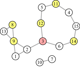
Figure 1: Graph for Example 1.

2.3 Examples

To motivate our results, we provide several explicit examples in this section.

A fertile source for compositional graphoids is of course graphical models. The following example will be used as a recurring example to illustrate our results (cf. Remark 1):

Example 1 (Graphical models).

Consider the graph $G$ shown in Figure 1 with $d=15$ nodes. We can associate to $G$ the corresponding separation graphoid $\mathcal{I}(G)$. Moreover, we can ensure this is probabilistically representable (it is even $\Sigma$-representable) by taking $\nu$ to be a Gaussian $\mathcal{N}(0,\Sigma)$ that is faithful to $G$. Such a Gaussian always exists [LM07], and in fact, this is generically true [AAZ22].

Although our main interest is in compositional graphoids that are not graphically or even probabilistically representable, for pedagogical reasons, it is useful to have a graph to visualize the CI relationships in terms of separation in $G$, so we will use the previous example as a running example in the sequel.

Below we provide some more general examples.

Example 2 (A compositional graphoid that is not probabilistically representable).

[Stu89] gave the following example of a graphoid that is not probabilistically representable. Consider a ground set with four elements, $V=\{a,b,c,d\}$. We use generic letters to denote each element in order to avoid associating this example with any random vector or distribution. Then $\mathcal{I}$ is defined by the following relations combined with their symmetric counterparts:

$$a\mathchoice{\mathrel{\hbox to0.0pt{$\displaystyle\perp$\hss}\mkern 4.0mu{\displaystyle\perp}}}{\mathrel{\hbox to0.0pt{$\textstyle\perp$\hss}\mkern 4.0mu{\textstyle\perp}}}{\mathrel{\hbox to0.0pt{$\scriptstyle\perp$\hss}\mkern 4.0mu{\scriptstyle\perp}}}{\mathrel{\hbox to0.0pt{$\scriptscriptstyle\perp$\hss}\mkern 4.0mu{\scriptscriptstyle\perp}}}b\,\mid\,\{c,d\},\quad c\mathchoice{\mathrel{\hbox to0.0pt{$\displaystyle\perp$\hss}\mkern 4.0mu{\displaystyle\perp}}}{\mathrel{\hbox to0.0pt{$\textstyle\perp$\hss}\mkern 4.0mu{\textstyle\perp}}}{\mathrel{\hbox to0.0pt{$\scriptstyle\perp$\hss}\mkern 4.0mu{\scriptstyle\perp}}}{\mathrel{\hbox to0.0pt{$\scriptscriptstyle\perp$\hss}\mkern 4.0mu{\scriptscriptstyle\perp}}}d\,\mid\,a,\quad c\mathchoice{\mathrel{\hbox to0.0pt{$\displaystyle\perp$\hss}\mkern 4.0mu{\displaystyle\perp}}}{\mathrel{\hbox to0.0pt{$\textstyle\perp$\hss}\mkern 4.0mu{\textstyle\perp}}}{\mathrel{\hbox to0.0pt{$\scriptstyle\perp$\hss}\mkern 4.0mu{\scriptstyle\perp}}}{\mathrel{\hbox to0.0pt{$\scriptscriptstyle\perp$\hss}\mkern 4.0mu{\scriptscriptstyle\perp}}}d\,\mid\,b,\quad a\mathchoice{\mathrel{\hbox to0.0pt{$\displaystyle\perp$\hss}\mkern 4.0mu{\displaystyle\perp}}}{\mathrel{\hbox to0.0pt{$\textstyle\perp$\hss}\mkern 4.0mu{\textstyle\perp}}}{\mathrel{\hbox to0.0pt{$\scriptstyle\perp$\hss}\mkern 4.0mu{\scriptstyle\perp}}}{\mathrel{\hbox to0.0pt{$\scriptscriptstyle\perp$\hss}\mkern 4.0mu{\scriptscriptstyle\perp}}}b,\quad A\mathchoice{\mathrel{\hbox to0.0pt{$\displaystyle\perp$\hss}\mkern 4.0mu{\displaystyle\perp}}}{\mathrel{\hbox to0.0pt{$\textstyle\perp$\hss}\mkern 4.0mu{\textstyle\perp}}}{\mathrel{\hbox to0.0pt{$\scriptstyle\perp$\hss}\mkern 4.0mu{\scriptstyle\perp}}}{\mathrel{\hbox to0.0pt{$\scriptscriptstyle\perp$\hss}\mkern 4.0mu{\scriptscriptstyle\perp}}}\emptyset\,\mid\,C,$$

In the last display, $A,C\subset V$ and $A\cap C=\emptyset$. Then it is easy to check that this defines a compositional graphoid. That it cannot be represented by any distribution follows from Proposition 5 in [Stu89].

Example 3 (Gaussoids that are not UGs).

[LM07] constructed examples of Gaussoids that are not $\Sigma$-representable. Suppose any such Gaussoid $\mathcal{I}$ was in fact repesented by a UG, so there is some UG $G$ such that $\mathcal{I}=\mathcal{I}(G)$. Then, by another result of [LM07, Corollary 3], we could find a Gaussian $\nu=\mathcal{N}(0,\Sigma)$ such that $\mathcal{I}(\nu)=\mathcal{I}(G)$, which contradicts the fact that $\mathcal{I}$ is not Gaussian (i.e. $\Sigma$-representable). As a result, Gaussoids can furnish examples of non-graphical, compositional graphoids.

Another rich source of examples is graphoids that can be represented by some graphical structure, but not others (e.g. by separation in an UG but not $d$-separation in a DAG or vice versa). Strictly speaking, such examples are indeed graphical (in the general sense according to Remark 1), however, in practice it can be difficult to know what kind of graphical model to use in any given context. Relaxing this requirement is one of the advantages of our approach, and we conclude this section with two examples below. These examples assume familiarity with graphical concepts such as $d$-separation, chain graphs, and mixed graphs. Since these concepts will not be needed anywhere else in the sequel, the uninitiated reader is referred to [Lau96] for the appropriate definitions.

(a) Chain graph in Example 4.

(b) Hidden variable model in Example 5.

Figure 2: Examples.

Example 4 (A chain graph that is not a DAG or UG).

Consider the chain graph in Figure 2(a), which is just the union of two subgraphs: A directed $v$-structure (red) and an undirected “diamond” (black). To distinguish between undirected separation and directed separation—a.k.a. $d$-separation—define the $d$-separation graphoid of a DAG to be the graphoid defined by $d$-separation. It is a standard fact about graphical models that there is no undirected graph whose separation graphoid represents the $d$-separation graphoid of a $v$-structure, and similarly there is no DAG whose $d$-separation graphoid represents the separation graphoid of a diamond. It follows that there is no undirected graph nor a directed acyclic graph $G$ such that $\mathcal{I}(G)=\mathcal{I}(\nu)$. See Example 14 for more on this model, after the main ideas have been introduced.

Example 5 (A mixed graph that is not a DAG or UG).

Another example comes from causal inference, where we model the effect of marginalizing a hidden variable. Consider the DAG in Figure 2(b). Let $\nu$ denote the law of $(X_{1},X_{2},X_{3},X_{4},H)$ and $Q_{H}$ the law of $(X_{1},X_{2},X_{3},X_{4})$ (i.e. after marginalizing $H$). Then it is well-known that there is no DAG or UG that is a perfect map of $Q_{H}$. The graphoid $\mathcal{I}(Q_{H})$ can be represented as a mixed graph, however.

3 Neighbourhood lattices and conditional independence

Let $V$ be fixed and $\mathcal{I}$ be a graphoid over $V$. In deliberate analogy with the usual convention for graphical models, we write $j\in V$ for general elements of the ground set, which will henceforth be referred to as nodes. Throughout the remainder of this section, we assume we are working with a fixed graphoid $\mathcal{I}$.

3.1 Relative Markov boundaries and blankets

The Markov boundary of an element $j$ in a graphoid is defined as the smallest subset $U\subset V_{-j}$ such that $j\mathchoice{\mathrel{\hbox to0.0pt{$\displaystyle\perp$\hss}\mkern 4.0mu{\displaystyle\perp}}}{\mathrel{\hbox to0.0pt{$\textstyle\perp$\hss}\mkern 4.0mu{\textstyle\perp}}}{\mathrel{\hbox to0.0pt{$\scriptstyle\perp$\hss}\mkern 4.0mu{\scriptstyle\perp}}}{\mathrel{\hbox to0.0pt{$\scriptscriptstyle\perp$\hss}\mkern 4.0mu{\scriptscriptstyle\perp}}}V_{-j}-U\,\mid\,U$ [PP85, Pea88]. By restricting $U$ to a given subset $S\subset V_{-j}$, we define the relative Markov boundary of $j$ in (or with respect to) $S$ as

$$m(j;S) =\bigcap\big{\{}U\subset S:\;j\mathchoice{\mathrel{\hbox to0.0pt{$\displaystyle\perp$\hss}\mkern 4.0mu{\displaystyle\perp}}}{\mathrel{\hbox to0.0pt{$\textstyle\perp$\hss}\mkern 4.0mu{\textstyle\perp}}}{\mathrel{\hbox to0.0pt{$\scriptstyle\perp$\hss}\mkern 4.0mu{\scriptstyle\perp}}}{\mathrel{\hbox to0.0pt{$\scriptscriptstyle\perp$\hss}\mkern 4.0mu{\scriptscriptstyle\perp}}}S-U\,\mid\,U\big{\}}.$$ (2)

In the sequel, we will frequently drop the qualifier “relative” when the context is clear, and use the more common “Markov boundary”, or even just “boundary” for brevity. The boundary $m(j;S)$ is well-defined, for any $S$, over any graphoid; this follows from the intersection axiom (G6). It also follows from the following more general result, which will be used repeatedly in the sequel. First, define for any subset $S\subset V$,

$$\mathfrak{t}_{j}(S)=\{U\subset S:\;j\mathchoice{\mathrel{\hbox to0.0pt{$\displaystyle\perp$\hss}\mkern 4.0mu{\displaystyle\perp}}}{\mathrel{\hbox to0.0pt{$\textstyle\perp$\hss}\mkern 4.0mu{\textstyle\perp}}}{\mathrel{\hbox to0.0pt{$\scriptstyle\perp$\hss}\mkern 4.0mu{\scriptstyle\perp}}}{\mathrel{\hbox to0.0pt{$\scriptscriptstyle\perp$\hss}\mkern 4.0mu{\scriptscriptstyle\perp}}}S-U\,\mid\,U\}.$$ (3)

Recall that a Markov blanket of $j\in V$ is any set $U$ such that $j\mathchoice{\mathrel{\hbox to0.0pt{$\displaystyle\perp$\hss}\mkern 4.0mu{\displaystyle\perp}}}{\mathrel{\hbox to0.0pt{$\textstyle\perp$\hss}\mkern 4.0mu{\textstyle\perp}}}{\mathrel{\hbox to0.0pt{$\scriptstyle\perp$\hss}\mkern 4.0mu{\scriptstyle\perp}}}{\mathrel{\hbox to0.0pt{$\scriptscriptstyle\perp$\hss}\mkern 4.0mu{\scriptscriptstyle\perp}}}V_{-j}-U\,\mid\,U$. Thus $\mathfrak{t}_{j}(S)$ is the collection of relative Markov blankets of $X_{j}$ with respect to the smaller ground set $S$. The following lemma shows that $\mathfrak{t}_{j}(S)$ is a convex lattice:

Lemma 1.

Let $\mathcal{I}$ be a graphoid over $V$, $j\in V$, and $S\subset V_{-j}$. Then $\mathfrak{t}_{j}(S)$ is an interval in $\mathfrak{B}(V_{-j})$, and hence in particular a convex lattice.

It follows that $\mathfrak{t}_{j}(S)$ has a well-defined infimum, i.e., (2) is well-defined and

$$m(j;S)=\inf\mathfrak{t}_{j}(S).$$

We also have the explicit interval representation $\mathfrak{t}_{j}(S)=[m(j;S),S]$. This follows since $S\in\mathfrak{t}_{j}(S)$ by definition, hence $S$ has to be the largest element of $\mathfrak{t}_{j}(S)$.

Example 6.

Consider the graph $G$ shown in Figure 1. For $j=3$, it is straightforward to compute various (relative) Markov boundaries of $j$ in the graphoid $\mathcal{I}(G)$:

$$S_{1}=V_{-j} \quad:\quad m(j;S_{1})=\{2,6,12\},$$

$$S_{2}=\{2,6,12\} \quad:\quad m(j;S_{2})=\{2,6,12\},$$

$$S_{3}=\{4,6,12,14\} \quad:\quad m(j;S_{3})=\{6,12\},$$

$$S_{4}=\{7,10\} \quad:\quad m(j;S_{4})=\emptyset,$$

$$S_{5}=\{8,9,11,12,14\} \quad:\quad m(j;S_{5})=\{9,12,14\}.$$

In each case, $m(j;S)$ is the smallest set $m\subset S$ separating $j$ from $S-m$.

3.2 The neighbourhood lattice

Recall the definition of the boundary $m(j;S)$ in (2).

Definition 1.

Given a compositional graphoid $\mathcal{I}$, a node $j\in V$, and $S\subset V$, define the neighbourhood lattice of $j$ relative to $S$ as

$$\mathfrak{T}_{j}(S) =\{U\subset V_{-j}:\;m(j;U)=m(j;S)\}.$$ (4)

In words, $\mathfrak{T}_{j}(S)$ is the collection of sets $U$ with respect to which $j$ has the same boundary as that with respect to $S$. When we wish to emphasize the underlying graphoid $\mathcal{I}$, we will write $\mathfrak{T}_{j}(S;\mathcal{I})$; this dependence will typically be suppressed otherwise.

It follows from Lemma 1 that $\mathfrak{T}_{j}(S)$ is well-defined. Our first main result establishes the most useful properties of the neighbourhood lattice; first and foremost, that it is indeed a lattice:

Theorem 1.

Let $\mathcal{I}$ be a compositional graphoid over $V$ and $j\in V$, $S\subset V_{-j}$ be fixed. Then:

1. $\mathfrak{T}_{j}(S)$ is an interval in $\mathfrak{B}(V_{-j})$, and in particular a convex sublattice of it.

2. $\inf\mathfrak{T}_{j}(S)=m(j;S)$;

3. $\sup\mathfrak{T}_{j}(S)=m(j;S)\cup E$ where $E=\{k\in V_{-j}:k\mathchoice{\mathrel{\hbox to0.0pt{$\displaystyle\perp$\hss}\mkern 4.0mu{\displaystyle\perp}}}{\mathrel{\hbox to0.0pt{$\textstyle\perp$\hss}\mkern 4.0mu{\textstyle\perp}}}{\mathrel{\hbox to0.0pt{$\scriptstyle\perp$\hss}\mkern 4.0mu{\scriptstyle\perp}}}{\mathrel{\hbox to0.0pt{$\scriptscriptstyle\perp$\hss}\mkern 4.0mu{\scriptscriptstyle\perp}}}j\,\mid\,m(j;S)\}$;

4. The neighbourhood lattices $\mathfrak{T}_{j}(S)$ partition the subset lattice $\mathfrak{B}(V_{-j})$; more precisely

   $$2^{V_{-j}}=\biguplus\big{\{}\mathfrak{T}_{j}(m):\;\text{$m=m(j;T)$ for some $T\subset V_{-j}$}\big{\}}.$$ (5)

The proof of Theorem 1 can be found in Section 3.5, after discussing the significance and various implications of this theorem.

Remark 2.

Inspection of the proof of Theorem 1 shows that if the graphoid $\mathcal{I}$ is not compositional (i.e. fails to satisfy (G7)), then $\mathfrak{T}_{j}(S)$ is still closed under set intersections and possesses the convexity property. The composition is only needed for closeness under set unions. Thus, in any graphoid, $\mathfrak{T}_{j}(S)$ is guaranteed to be at least a meet semi-sublattice of $\mathfrak{B}(V_{-j})$.

Since $\mathfrak{T}_{j}(S)$ is a lattice, it has a well-defined infimum and supremum. Theorem 1(b) characterizes the infimum of $\mathfrak{T}_{j}(S)$ as the Markov boundary of $j$ in $S$. The supremum also plays an important role, which we denote by $M(j;S)$:

$$M(j;S):=\sup\mathfrak{T}_{j}(S).$$ (6)

Theorem 1(c) characterizes this supremum by adding to the infimum $m:=m(j;S)$ every node $k$ that is independent of $j$ given $m$ (in graphical terms, $m$ separates $j$ and $k$).

Example 7.

Continuing Example 6, we have the following:

$$S_{1}=V_{-j} \quad:\quad M(j;S_{1})=V_{-j}\implies\mathfrak{T}_{j}(S_{1})=[\{2,6,12\},V_{-j}],$$

$$S_{2}=\{2,6,12\} \quad:\quad M(j;S_{2})=V_{-j}\implies\mathfrak{T}_{j}(S_{2})=[\{2,6,12\},V_{-j}],$$

$$S_{3}=\{4,6,12,14\} \quad:\quad M(j;S_{3})=\{4,5,6,7,10,11,12,14,15\}$$

$$\qquad\qquad\implies\mathfrak{T}_{j}(S_{3})=[\{6,12\},\{4,5,6,7,10,11,12,14,15\}]$$

$$S_{4}=\{7,10\} \quad:\quad M(j;S_{4})=S_{4}\implies\mathfrak{T}_{j}(S_{4})=[\emptyset,S_{4}].$$

$$S_{5}=\{8,9,11,12,14\} \quad:\quad M(j;S_{5})=\{4,5,7,8,9,10,11,12,13,14,15\}$$

$$\qquad\qquad\implies\mathfrak{T}_{j}(S_{5})=[\{9,12,14\},\{4,5,7,8,9,10,11,12,13,14,15\}].$$

These are obtained by noting that in a separation graphoid, the supremum $M(j;S)$ can be easily read from the graph by adding to $m(j;S)$ every node in $V_{-j}$ that is separated from $j$ by $m(j;S)$; see Section 6 for details. By the convexity of these lattices, we immediately conclude for example that both $\{2,6,7,10,12\}$ and $\{2,6,8,9,12\}$ belong to $\mathfrak{T}_{j}(V_{-j})$. Note that these two sets are not comparable in $2^{V_{-j}}$, i.e., the neighbourhood lattice $\mathfrak{T}_{j}(V_{-j})$ is not a chain (or totally ordered set) in $2^{V_{-j}}$. In this case, $\mathfrak{T}_{j}(V_{-j})$ contains $2^{|M_{j}|-|m_{j}|}=2^{11}$ subsets, out of a total possible $|2^{[15]_{3}}|=2^{14}$. The Markov boundary for $j=3$ given any of these subsets is thus the same. For a more extreme example, a similar calculation shows that $|\mathfrak{T}_{j}(S_{5})|=2^{8}=256$ out of $2^{14}$ possible subsets.

Finally, before concluding this section, we provide a detailed accounting of different equivalent representations of the neighbourhood lattice:

Theorem 2.

The following definitions of $\mathfrak{T}_{j}(S)$ are equivalent:

1. $\mathfrak{T}_{j}(S)=\{U\subset V_{-j}:m(j;U)=m(j;S)\}=\{U\subset V_{-j}:\inf\mathfrak{t}_{j}(U)=\inf\mathfrak{t}_{j}(S)\}$;

2. $\mathfrak{T}_{j}(S)=\bigcup\{\mathfrak{t}_{j}(U):\inf\mathfrak{t}_{j}(U)=\inf\mathfrak{t}_{j}(S)\}$, i.e. $\mathfrak{T}_{j}(S)$ is maximal amongst the lattices $\mathfrak{t}_{j}(S)$ with the same minimal element;

3. $\mathfrak{T}_{j}(S)=\{U\subset S:j\mathchoice{\mathrel{\hbox to0.0pt{$\displaystyle\perp$\hss}\mkern 4.0mu{\displaystyle\perp}}}{\mathrel{\hbox to0.0pt{$\textstyle\perp$\hss}\mkern 4.0mu{\textstyle\perp}}}{\mathrel{\hbox to0.0pt{$\scriptstyle\perp$\hss}\mkern 4.0mu{\scriptstyle\perp}}}{\mathrel{\hbox to0.0pt{$\scriptscriptstyle\perp$\hss}\mkern 4.0mu{\scriptscriptstyle\perp}}}S-U\,\mid\,U\}\cup\{U\supset S:j\mathchoice{\mathrel{\hbox to0.0pt{$\displaystyle\perp$\hss}\mkern 4.0mu{\displaystyle\perp}}}{\mathrel{\hbox to0.0pt{$\textstyle\perp$\hss}\mkern 4.0mu{\textstyle\perp}}}{\mathrel{\hbox to0.0pt{$\scriptstyle\perp$\hss}\mkern 4.0mu{\scriptstyle\perp}}}{\mathrel{\hbox to0.0pt{$\scriptscriptstyle\perp$\hss}\mkern 4.0mu{\scriptscriptstyle\perp}}}U-S\,\mid\,S\}$;

4. $\mathfrak{T}_{j}(S)=\mathfrak{t}_{j}(S)\cup\{A\cup B:A\cap B=\emptyset,\,A\in\mathfrak{t}_{j}(S),\,j\mathchoice{\mathrel{\hbox to0.0pt{$\displaystyle\perp$\hss}\mkern 4.0mu{\displaystyle\perp}}}{\mathrel{\hbox to0.0pt{$\textstyle\perp$\hss}\mkern 4.0mu{\textstyle\perp}}}{\mathrel{\hbox to0.0pt{$\scriptstyle\perp$\hss}\mkern 4.0mu{\scriptstyle\perp}}}{\mathrel{\hbox to0.0pt{$\scriptscriptstyle\perp$\hss}\mkern 4.0mu{\scriptscriptstyle\perp}}}B\,\mid\,A\}$;

5. $\mathfrak{T}_{j}(S)=[m,M]$, where $m\subset V$ is the smallest subset such that $j\mathchoice{\mathrel{\hbox to0.0pt{$\displaystyle\perp$\hss}\mkern 4.0mu{\displaystyle\perp}}}{\mathrel{\hbox to0.0pt{$\textstyle\perp$\hss}\mkern 4.0mu{\textstyle\perp}}}{\mathrel{\hbox to0.0pt{$\scriptstyle\perp$\hss}\mkern 4.0mu{\scriptstyle\perp}}}{\mathrel{\hbox to0.0pt{$\scriptscriptstyle\perp$\hss}\mkern 4.0mu{\scriptscriptstyle\perp}}}S-m\,\mid\,m$ and $M\subset V$ is the largest subset such that $j\mathchoice{\mathrel{\hbox to0.0pt{$\displaystyle\perp$\hss}\mkern 4.0mu{\displaystyle\perp}}}{\mathrel{\hbox to0.0pt{$\textstyle\perp$\hss}\mkern 4.0mu{\textstyle\perp}}}{\mathrel{\hbox to0.0pt{$\scriptstyle\perp$\hss}\mkern 4.0mu{\scriptstyle\perp}}}{\mathrel{\hbox to0.0pt{$\scriptscriptstyle\perp$\hss}\mkern 4.0mu{\scriptscriptstyle\perp}}}M-S\,\mid\,S$.

6. $\mathfrak{T}_{j}(S)=\{T\subset V_{-j}:j\mathchoice{\mathrel{\hbox to0.0pt{$\displaystyle\perp$\hss}\mkern 4.0mu{\displaystyle\perp}}}{\mathrel{\hbox to0.0pt{$\textstyle\perp$\hss}\mkern 4.0mu{\textstyle\perp}}}{\mathrel{\hbox to0.0pt{$\scriptstyle\perp$\hss}\mkern 4.0mu{\scriptstyle\perp}}}{\mathrel{\hbox to0.0pt{$\scriptscriptstyle\perp$\hss}\mkern 4.0mu{\scriptscriptstyle\perp}}}T-m(j;S)\,\mid\,m(j;S)\}$.

Furthermore, we have the following property:

1. $\mathfrak{T}_{j}(S)=\mathfrak{T}_{j}(T)$ for all $T\in\mathfrak{T}_{j}(S)=[m,M]$ as in (A5).

In light of Theorem 1, the proof of these equivalences is a straightforward manipulation of the definitions, and hence is omitted.

3.3 Implications for conditional independence

As our first application, we illustrate how these neighbourbood lattices can be used to check arbitrary relations of the form $A\mathchoice{\mathrel{\hbox to0.0pt{$\displaystyle\perp$\hss}\mkern 4.0mu{\displaystyle\perp}}}{\mathrel{\hbox to0.0pt{$\textstyle\perp$\hss}\mkern 4.0mu{\textstyle\perp}}}{\mathrel{\hbox to0.0pt{$\scriptstyle\perp$\hss}\mkern 4.0mu{\scriptstyle\perp}}}{\mathrel{\hbox to0.0pt{$\scriptscriptstyle\perp$\hss}\mkern 4.0mu{\scriptscriptstyle\perp}}}B\,\mid\,C$. As a practical use case for these results, consider when $\mathcal{I}=\mathcal{I}(\nu)$ is a compositional probabilistic graphoid, in which case $A\mathchoice{\mathrel{\hbox to0.0pt{$\displaystyle\perp$\hss}\mkern 4.0mu{\displaystyle\perp}}}{\mathrel{\hbox to0.0pt{$\textstyle\perp$\hss}\mkern 4.0mu{\textstyle\perp}}}{\mathrel{\hbox to0.0pt{$\scriptstyle\perp$\hss}\mkern 4.0mu{\scriptstyle\perp}}}{\mathrel{\hbox to0.0pt{$\scriptscriptstyle\perp$\hss}\mkern 4.0mu{\scriptscriptstyle\perp}}}B\,\mid\,C$ corresponds to conditional independence in the distribution $\nu$.

Our first result relates so-called elementary CI relations of the form $j\mathchoice{\mathrel{\hbox to0.0pt{$\displaystyle\perp$\hss}\mkern 4.0mu{\displaystyle\perp}}}{\mathrel{\hbox to0.0pt{$\textstyle\perp$\hss}\mkern 4.0mu{\textstyle\perp}}}{\mathrel{\hbox to0.0pt{$\scriptstyle\perp$\hss}\mkern 4.0mu{\scriptstyle\perp}}}{\mathrel{\hbox to0.0pt{$\scriptscriptstyle\perp$\hss}\mkern 4.0mu{\scriptscriptstyle\perp}}}i\,\mid\,C$ to inclusion in the lattice $\mathfrak{T}_{j}(S)$:

Corollary 1.

Let $\mathcal{I}$ be a compositional graphoid over $V,$ $C\subset V,$ and $i,j\in V-C$. Then the following statements are equivalent:

1. $j\mathchoice{\mathrel{\hbox to0.0pt{$\displaystyle\perp$\hss}\mkern 4.0mu{\displaystyle\perp}}}{\mathrel{\hbox to0.0pt{$\textstyle\perp$\hss}\mkern 4.0mu{\textstyle\perp}}}{\mathrel{\hbox to0.0pt{$\scriptstyle\perp$\hss}\mkern 4.0mu{\scriptstyle\perp}}}{\mathrel{\hbox to0.0pt{$\scriptscriptstyle\perp$\hss}\mkern 4.0mu{\scriptscriptstyle\perp}}}i\,\mid\,C$;

2. There is a neighbourhood lattice $\mathfrak{T}_{j}(S)=[m,M]$ such that $i\in M-m$ and $C\in[m,M-i]$;

3. $C\in\mathfrak{T}_{j}(Ci)$;

4. $m(j;Ci)\subset C$.

The proof is an easy application of the definitions.

Next, in order to check general relations $A\mathchoice{\mathrel{\hbox to0.0pt{$\displaystyle\perp$\hss}\mkern 4.0mu{\displaystyle\perp}}}{\mathrel{\hbox to0.0pt{$\textstyle\perp$\hss}\mkern 4.0mu{\textstyle\perp}}}{\mathrel{\hbox to0.0pt{$\scriptstyle\perp$\hss}\mkern 4.0mu{\scriptstyle\perp}}}{\mathrel{\hbox to0.0pt{$\scriptscriptstyle\perp$\hss}\mkern 4.0mu{\scriptscriptstyle\perp}}}B\,\mid\,C$, we can use decomposition (G3) and composition (G7) to prove the following (see also Corollary 1 in [LS18]):

Corollary 2.

Let $\mathcal{I}$ be a compositional graphoid over $V,$ and $A,B,C$ disjoint subsets of $V.$ Then $A\mathchoice{\mathrel{\hbox to0.0pt{$\displaystyle\perp$\hss}\mkern 4.0mu{\displaystyle\perp}}}{\mathrel{\hbox to0.0pt{$\textstyle\perp$\hss}\mkern 4.0mu{\textstyle\perp}}}{\mathrel{\hbox to0.0pt{$\scriptstyle\perp$\hss}\mkern 4.0mu{\scriptstyle\perp}}}{\mathrel{\hbox to0.0pt{$\scriptscriptstyle\perp$\hss}\mkern 4.0mu{\scriptscriptstyle\perp}}}B\,\mid\,C$ if and only if

$$C\in\bigcap_{a\in A}\bigcap_{b\in B}\mathfrak{T}_{b}(Ca),$$ (7)

or equivalently,

$$\bigcup_{a\in A}\bigcup_{b\in B}m(a;Cb)\subset C.$$ (8)

The special case of (8) when $A=j$ and $B=i$, i.e. checking an elementary CI relation, is equivalent to Corollary 1(d). In this case, $j\mathchoice{\mathrel{\hbox to0.0pt{$\displaystyle\perp$\hss}\mkern 4.0mu{\displaystyle\perp}}}{\mathrel{\hbox to0.0pt{$\textstyle\perp$\hss}\mkern 4.0mu{\textstyle\perp}}}{\mathrel{\hbox to0.0pt{$\scriptstyle\perp$\hss}\mkern 4.0mu{\scriptstyle\perp}}}{\mathrel{\hbox to0.0pt{$\scriptscriptstyle\perp$\hss}\mkern 4.0mu{\scriptscriptstyle\perp}}}i\,\mid\,C$ if and only if

$$m(j;Ci)=\inf\mathfrak{T}_{j}(Ci)\subset C.$$ (9)

Thus, Corollaries 1 and 2 establish an explicit connection between the neighbourhood lattice and conditional independence: In one direction, an elementary CI relation $i\mathchoice{\mathrel{\hbox to0.0pt{$\displaystyle\perp$\hss}\mkern 4.0mu{\displaystyle\perp}}}{\mathrel{\hbox to0.0pt{$\textstyle\perp$\hss}\mkern 4.0mu{\textstyle\perp}}}{\mathrel{\hbox to0.0pt{$\scriptstyle\perp$\hss}\mkern 4.0mu{\scriptstyle\perp}}}{\mathrel{\hbox to0.0pt{$\scriptscriptstyle\perp$\hss}\mkern 4.0mu{\scriptscriptstyle\perp}}}j\,\mid\,C$ can be verified by checking the inclusion (9), which can then be used to check arbitrary CI relations via (8). In the other direction, given the lattice $\mathfrak{T}_{j}(S)=[m,M]$, we may immediately conclude that $j\mathchoice{\mathrel{\hbox to0.0pt{$\displaystyle\perp$\hss}\mkern 4.0mu{\displaystyle\perp}}}{\mathrel{\hbox to0.0pt{$\textstyle\perp$\hss}\mkern 4.0mu{\textstyle\perp}}}{\mathrel{\hbox to0.0pt{$\scriptstyle\perp$\hss}\mkern 4.0mu{\scriptstyle\perp}}}{\mathrel{\hbox to0.0pt{$\scriptscriptstyle\perp$\hss}\mkern 4.0mu{\scriptscriptstyle\perp}}}i\,\mid\,C$ for all $i\in M-m$ and $C\in[m,M-i]$.

The next example illustrates these results. We assume for now that we can compute the corresponding boundaries and neighbourhood lattices; this will be taken up in Sections 4 and 6.

Example 8.

Reading off the graph in Example 6 (see Figure 1), we can see that $X_{3}\mathchoice{\mathrel{\hbox to0.0pt{$\displaystyle\perp$\hss}\mkern 4.0mu{\displaystyle\perp}}}{\mathrel{\hbox to0.0pt{$\textstyle\perp$\hss}\mkern 4.0mu{\textstyle\perp}}}{\mathrel{\hbox to0.0pt{$\scriptstyle\perp$\hss}\mkern 4.0mu{\scriptstyle\perp}}}{\mathrel{\hbox to0.0pt{$\scriptscriptstyle\perp$\hss}\mkern 4.0mu{\scriptscriptstyle\perp}}}X_{9}\,\mid\,(X_{1},X_{2})$ and $(X_{1},X_{2})\mathchoice{\mathrel{\hbox to0.0pt{$\displaystyle\perp$\hss}\mkern 4.0mu{\displaystyle\perp}}}{\mathrel{\hbox to0.0pt{$\textstyle\perp$\hss}\mkern 4.0mu{\textstyle\perp}}}{\mathrel{\hbox to0.0pt{$\scriptstyle\perp$\hss}\mkern 4.0mu{\scriptstyle\perp}}}{\mathrel{\hbox to0.0pt{$\scriptscriptstyle\perp$\hss}\mkern 4.0mu{\scriptscriptstyle\perp}}}(X_{8},X_{13})\,\mid\,X_{9}$ in the separation graphoid $\mathcal{I}(G)$. To check these via the corresponding neighbourhood lattice it suffices to check (8) or (9). For example, in the first relation we have $j=3$, $i=9$, $C=\{1,2\}$, and

$$m(j;Ci)=m(3;\{1,2,9\})=\{1,2\}\subset C=\{1,2\}.$$

This confirms (9), as expected. For the second relation, we need to check four lattices, as follows:

$$\bigcup_{a\in A}\bigcup_{b\in B}m(a;Cb) =\bigcup_{a\in\{1,2\}}\bigcup_{b\in\{8,13\}}m(a;Cb)$$

$$=m(1;\{8,9\})\cup m(1;\{9,13\})\cup m(2;\{8,9\})\cup m(2;\{9,13\})$$

$$=\{9\}\cup\{9\}\cup\{9\}\cup\{9\}$$

$$\subset C=\{9\},$$

which confirms (8).

3.4 The neighbourhood lattice decomposition

The decomposition (5) and its connection with conditional independence through Corollaries 1 and 2 motivate the following definition:

Definition 2.

The neighbourhood lattice decomposition $\mathfrak{D}_{j}$ of $j\in V$ is the partition of $\mathfrak{B}(V_{-j})$ given by Theorem 1(d). More precisely,

$$\mathfrak{D}_{j}=\big{\{}\mathfrak{T}_{j}(m):\text{$m=m(j;S)$ for some $S\subset V_{-j}$}\big{\}}.$$ (10)

When the node $j$ is clear from the context we will often suppress this argument and simply write $\mathfrak{D}$. By (5), we have $2^{V_{-j}}=\bigcup\mathfrak{D}$.

We can think of the neighbourhood lattice decomposition of $j\in V$ as a compact encoding of the local conditional independence structure of $j$. For example, all of the elementary CI statements involving node $j$ can be listed as follows: Let $\mathfrak{D}=\{\mathfrak{T}^{1},\ldots,\mathfrak{T}^{k}\}$ denote the neighbourhood lattice decomposition for $j$, where we have suppressed the index $j$ to avoid notational clutter. Write $\mathfrak{T}^{\ell}=[m^{\ell},M^{\ell}]$ for $\ell=1,\ldots,k$, so that we have

$$j\mathchoice{\mathrel{\hbox to0.0pt{$\displaystyle\perp$\hss}\mkern 4.0mu{\displaystyle\perp}}}{\mathrel{\hbox to0.0pt{$\textstyle\perp$\hss}\mkern 4.0mu{\textstyle\perp}}}{\mathrel{\hbox to0.0pt{$\scriptstyle\perp$\hss}\mkern 4.0mu{\scriptstyle\perp}}}{\mathrel{\hbox to0.0pt{$\scriptscriptstyle\perp$\hss}\mkern 4.0mu{\scriptscriptstyle\perp}}}i\,\mid\,C\quad\text{for all}\quad i\in M^{\ell}-m^{\ell},\quad C\in[m^{\ell},M^{\ell}_{-i}],\quad\ell=1,\dots,k.$$ (11)

The total number of CI statements in (11) is

$$\sum_{\ell=1}^{k}\big{(}|M^{\ell}|-|m^{\ell}|\big{)}\,2^{|M^{\ell}|-|m^{\ell}|-1},$$ (12)

where $|M^{\ell}|$ is the cardinality of set $M^{\ell}$ and so on. The total number of disjoint triplets $(j,i,C)$ involving a fixed node $j$ is $(d-1)2^{d-2}$. According to Corollary 1(a), there is no double-counting in (11) and all the CI statements (involving $j$) are accounted for. Thus, in the absence of a graphical representation, the lattice decomposition provides an alternative “economical encoding” of CI statements with the potential for substantial savings over simply listing all possible graphoid relations. The following example illustrates this; once again, we take for granted the computations to be in introduced in Sections 4 and 6.

Example 9.

Continuing Examples 6 and 7, we compute the neighbourhood lattice decomposition $\mathfrak{D}$ for node $j=3$. The decomposition turns out to have $K=319$ lattices. Tables 2 and 2 contain some statistics about this decomposition, namely, how many sets are covered by each lattice and the sizes of their minimum element (i.e., set $m$). For example, Table 2 shows that there are 5 lattices in the decomposition that cover $512$ sets each. Similarly, there are $21$ lattices whose minimal element is a set of size $5$ (Table 2).

											Total
Number of sets covered	4	8	16	32	64	128	256	512	1024	2048	$16384$
Number of lattices	112	40	60	34	38	19	8	5	2	1	$319$

Table 1: The distribution of the number of sets covered by each lattice $\mathfrak{T}=[m,M]$, i.e. $2^{|M|-|m|}$, for the setup of Example 9.

size of $m$	0	1	2	3	4	5
number of lattices	1	12	60	134	91	21

Table 2: The distribution of the size of the minimal element of the lattice $\mathfrak{T}=[m,M]$, i.e. set $m$, for the setup of Example 9.

Thus, the complexity of enumerating all CI statements boils down to the complexity of computing the lattice decomposition $\mathfrak{D}$. In Section 4, we analyze the complexity of computing an individual lattice $\mathfrak{T}_{j}(S)$ as well as the full lattice decomposition $\mathfrak{D}$, and give several practical algorithms for their computation.

3.5 Proof of Theorem 1

We now prove Theorem 1. First, we establish several simple lemmas that will prove useful. As a guide to the reader, Lemmas 2 and 4 below are intermediate, whereas Lemmas 3 and 5 are key lemmas that will be invoked in the main proof.

The following is an immediate consequence of decomposition (G3):

Lemma 2.

Let $m=\inf\mathfrak{t}_{j}(S)$. Then $j\mathchoice{\mathrel{\hbox to0.0pt{$\displaystyle\perp$\hss}\mkern 4.0mu{\displaystyle\perp}}}{\mathrel{\hbox to0.0pt{$\textstyle\perp$\hss}\mkern 4.0mu{\textstyle\perp}}}{\mathrel{\hbox to0.0pt{$\scriptstyle\perp$\hss}\mkern 4.0mu{\scriptstyle\perp}}}{\mathrel{\hbox to0.0pt{$\scriptscriptstyle\perp$\hss}\mkern 4.0mu{\scriptscriptstyle\perp}}}U-m\,\mid\,m$ for all $U\in\mathfrak{t}_{j}(S)$.

We will also need the following key technical lemma regarding $\mathfrak{t}_{j}(S)$:

Lemma 3.

For any $U\in\mathfrak{t}_{j}(S)$, we have $\inf\mathfrak{t}_{j}(U)=\inf\mathfrak{t}_{j}(S)$.

Proof.

Let $m_{0}=\inf\mathfrak{t}_{j}(U)$ and $m=\inf\mathfrak{t}_{j}(S)$. By Lemma 2, $j\mathchoice{\mathrel{\hbox to0.0pt{$\displaystyle\perp$\hss}\mkern 4.0mu{\displaystyle\perp}}}{\mathrel{\hbox to0.0pt{$\textstyle\perp$\hss}\mkern 4.0mu{\textstyle\perp}}}{\mathrel{\hbox to0.0pt{$\scriptstyle\perp$\hss}\mkern 4.0mu{\scriptstyle\perp}}}{\mathrel{\hbox to0.0pt{$\scriptscriptstyle\perp$\hss}\mkern 4.0mu{\scriptscriptstyle\perp}}}U-m\,\mid\,m$, whence $m\in\mathfrak{t}_{j}(U)$ by definition. Thus $m_{0}\subset m\subset U$. Since we have established $m\subset U$, by decomposition (G3), $j\mathchoice{\mathrel{\hbox to0.0pt{$\displaystyle\perp$\hss}\mkern 4.0mu{\displaystyle\perp}}}{\mathrel{\hbox to0.0pt{$\textstyle\perp$\hss}\mkern 4.0mu{\textstyle\perp}}}{\mathrel{\hbox to0.0pt{$\scriptstyle\perp$\hss}\mkern 4.0mu{\scriptstyle\perp}}}{\mathrel{\hbox to0.0pt{$\scriptscriptstyle\perp$\hss}\mkern 4.0mu{\scriptscriptstyle\perp}}}U-m_{0}\,\mid\,m_{0}$ implies $j\mathchoice{\mathrel{\hbox to0.0pt{$\displaystyle\perp$\hss}\mkern 4.0mu{\displaystyle\perp}}}{\mathrel{\hbox to0.0pt{$\textstyle\perp$\hss}\mkern 4.0mu{\textstyle\perp}}}{\mathrel{\hbox to0.0pt{$\scriptstyle\perp$\hss}\mkern 4.0mu{\scriptstyle\perp}}}{\mathrel{\hbox to0.0pt{$\scriptscriptstyle\perp$\hss}\mkern 4.0mu{\scriptscriptstyle\perp}}}m-m_{0}\,\mid\,m_{0}$. Combine this with $j\mathchoice{\mathrel{\hbox to0.0pt{$\displaystyle\perp$\hss}\mkern 4.0mu{\displaystyle\perp}}}{\mathrel{\hbox to0.0pt{$\textstyle\perp$\hss}\mkern 4.0mu{\textstyle\perp}}}{\mathrel{\hbox to0.0pt{$\scriptstyle\perp$\hss}\mkern 4.0mu{\scriptstyle\perp}}}{\mathrel{\hbox to0.0pt{$\scriptscriptstyle\perp$\hss}\mkern 4.0mu{\scriptscriptstyle\perp}}}S-m\,\mid\,(m-m_{0})\cup m_{0}$, using contraction (G5), to deduce $j\mathchoice{\mathrel{\hbox to0.0pt{$\displaystyle\perp$\hss}\mkern 4.0mu{\displaystyle\perp}}}{\mathrel{\hbox to0.0pt{$\textstyle\perp$\hss}\mkern 4.0mu{\textstyle\perp}}}{\mathrel{\hbox to0.0pt{$\scriptstyle\perp$\hss}\mkern 4.0mu{\scriptstyle\perp}}}{\mathrel{\hbox to0.0pt{$\scriptscriptstyle\perp$\hss}\mkern 4.0mu{\scriptscriptstyle\perp}}}S-m_{0}\,\mid\,m_{0}$. Here, we have used $(S-m)\cup(m-m_{0})=S-m_{0}$ which follows from $m_{0}\subset m\subset S$. Thus $m_{0}\in\mathfrak{t}_{j}(S)$, and hence $m\subset m_{0}$. We conclude that $m=m_{0}$, as desired. ∎

In the previous lemma, the condition $U\in\mathfrak{t}_{j}(S)$ cannot be removed, as the following example shows.

Example 10.

In general, if $U\subset S$, we will not even have $\inf\mathfrak{t}_{j}(U)\subset\inf\mathfrak{t}_{j}(S)$. To see this, consider the set $S_{3}=\{4,6,12,14\}$ and $j=3$ from Example 6, so that $\inf\mathfrak{t}_{j}(S_{3})=\{6,12\}$. Take $U=\{4,6,14\}\subset S_{3}$ and note that $U\notin\mathfrak{t}_{j}(S_{3})=[\{6,12\},\{4,6,12,14\}]$. We have $\inf\mathfrak{t}_{j}(U)=\{4,6\}$ which is incomparable to $\inf\mathfrak{t}_{j}(S_{3})$.

The next two lemmas, which are useful in their own right, illustrate how elements of $\mathfrak{T}_{j}(S)$ can be partitioned via knowledge of separation in the underlying graphoid. These results are crucial to property (c) in Theorem 1.

Lemma 4.

$T\in\mathfrak{T}_{j}(S)\implies\mathfrak{T}_{j}(S)=\mathfrak{T}_{j}(T)$.

Proof.

Since $T\in\mathfrak{T}_{j}(S)$, we have $m(j;S)=m(j;T)$. Now for any $A\in\mathfrak{T}_{j}(S)$ we have $m(j;A)=m(j;S)=m(j;T)$, whence $A\in\mathfrak{T}_{j}(T)$. Thus $\mathfrak{T}_{j}(S)\subset\mathfrak{T}_{j}(T)$, and similarly $\mathfrak{T}_{j}(T)\subset\mathfrak{T}_{j}(S)$. ∎

Lemma 5.

Fix $S\subset V_{-j}$ and let $A\subset V_{-j}$ and $B\in\mathfrak{T}_{j}(S)$ be disjoint. Then $j\mathchoice{\mathrel{\hbox to0.0pt{$\displaystyle\perp$\hss}\mkern 4.0mu{\displaystyle\perp}}}{\mathrel{\hbox to0.0pt{$\textstyle\perp$\hss}\mkern 4.0mu{\textstyle\perp}}}{\mathrel{\hbox to0.0pt{$\scriptstyle\perp$\hss}\mkern 4.0mu{\scriptstyle\perp}}}{\mathrel{\hbox to0.0pt{$\scriptscriptstyle\perp$\hss}\mkern 4.0mu{\scriptscriptstyle\perp}}}A\,\mid\,B$ if and only if $A\cup B\in\mathfrak{T}_{j}(S)$.

Proof.

Since $B\in\mathfrak{T}_{j}(S)$, we have $\mathfrak{T}_{j}(B)=\mathfrak{T}_{j}(S)$ by Lemma 4. Hence $A\cup B\in\mathfrak{T}_{j}(S)\iff A\cup B\in\mathfrak{T}_{j}(B)$, which is equivalent to $B\in\mathfrak{T}_{j}(A\cup B)$. But by definition this means

$$j\mathchoice{\mathrel{\hbox to0.0pt{$\displaystyle\perp$\hss}\mkern 4.0mu{\displaystyle\perp}}}{\mathrel{\hbox to0.0pt{$\textstyle\perp$\hss}\mkern 4.0mu{\textstyle\perp}}}{\mathrel{\hbox to0.0pt{$\scriptstyle\perp$\hss}\mkern 4.0mu{\scriptstyle\perp}}}{\mathrel{\hbox to0.0pt{$\scriptscriptstyle\perp$\hss}\mkern 4.0mu{\scriptscriptstyle\perp}}}(A\cup B)-B\,\mid\,B \iff j\mathchoice{\mathrel{\hbox to0.0pt{$\displaystyle\perp$\hss}\mkern 4.0mu{\displaystyle\perp}}}{\mathrel{\hbox to0.0pt{$\textstyle\perp$\hss}\mkern 4.0mu{\textstyle\perp}}}{\mathrel{\hbox to0.0pt{$\scriptstyle\perp$\hss}\mkern 4.0mu{\scriptstyle\perp}}}{\mathrel{\hbox to0.0pt{$\scriptscriptstyle\perp$\hss}\mkern 4.0mu{\scriptscriptstyle\perp}}}A\,\mid\,B.\qed$$

Finally, we proceed with the proof of Theorem 1.

Proof of Theorem 1.

We break the proof of (a) into three parts (i) Existence of meets, (ii) Existence of joins, and (iii) Convexity. Throughout, we assume that $T,R\in\mathfrak{T}_{j}(S)$. Then, by the definition of $\mathfrak{T}_{j}(S)$, we have $\inf\mathfrak{t}_{j}(T)=\inf\mathfrak{t}_{j}(R)=m$ for some set $m\subset T,R$. It follows that $\mathfrak{t}_{j}(T)=[m,T]$ and $\mathfrak{t}_{j}(R)=[m,R]$; see the discussion following Lemma 1.

(i) We wish to show that $T\cap R\in\mathfrak{T}_{j}(S)$. Since $m\subset T$ and $m\subset R$, it follows that $m\subset T\cap R\subset T$, whence $T\cap R\in\mathfrak{t}_{j}(T)$. Now apply Lemma 3 to deduce that $\inf\mathfrak{t}_{j}(T\cap R)=\inf\mathfrak{t}_{j}(T)=m$. Thus $T\cap R\in\mathfrak{T}_{j}(S)$.

(ii) We wish to show that $TR\in\mathfrak{T}_{j}(S)$. Since $T\in\mathfrak{t}_{j}(T)$ and $m=\inf\mathfrak{t}_{j}(T)$, Lemma 2 implies $j\mathchoice{\mathrel{\hbox to0.0pt{$\displaystyle\perp$\hss}\mkern 4.0mu{\displaystyle\perp}}}{\mathrel{\hbox to0.0pt{$\textstyle\perp$\hss}\mkern 4.0mu{\textstyle\perp}}}{\mathrel{\hbox to0.0pt{$\scriptstyle\perp$\hss}\mkern 4.0mu{\scriptstyle\perp}}}{\mathrel{\hbox to0.0pt{$\scriptscriptstyle\perp$\hss}\mkern 4.0mu{\scriptscriptstyle\perp}}}T-m\,\mid\,m$. Similarly, $j\mathchoice{\mathrel{\hbox to0.0pt{$\displaystyle\perp$\hss}\mkern 4.0mu{\displaystyle\perp}}}{\mathrel{\hbox to0.0pt{$\textstyle\perp$\hss}\mkern 4.0mu{\textstyle\perp}}}{\mathrel{\hbox to0.0pt{$\scriptstyle\perp$\hss}\mkern 4.0mu{\scriptstyle\perp}}}{\mathrel{\hbox to0.0pt{$\scriptscriptstyle\perp$\hss}\mkern 4.0mu{\scriptscriptstyle\perp}}}R-m\,\mid\,m$. By composition (G7), $j\mathchoice{\mathrel{\hbox to0.0pt{$\displaystyle\perp$\hss}\mkern 4.0mu{\displaystyle\perp}}}{\mathrel{\hbox to0.0pt{$\textstyle\perp$\hss}\mkern 4.0mu{\textstyle\perp}}}{\mathrel{\hbox to0.0pt{$\scriptstyle\perp$\hss}\mkern 4.0mu{\scriptstyle\perp}}}{\mathrel{\hbox to0.0pt{$\scriptscriptstyle\perp$\hss}\mkern 4.0mu{\scriptscriptstyle\perp}}}(TR)-m\,\mid\,m$, whence $m\in\mathfrak{t}_{j}(TR)$. Since both $m$ and $TR$ belong to $\mathfrak{t}_{j}(TR)$, and $m\subset T\subset TR$, it follows from the convexity of $\mathfrak{t}_{j}(TR)$ (Lemma 1) that $T\in\mathfrak{t}_{j}(TR)$. Applying Lemma 3, we have $\inf\mathfrak{t}_{j}(T)=\inf\mathfrak{t}_{j}(TR)$, the desired result.

(iii) Suppose $T\subset R$ and let $U$ satisfy $T\subset U\subset R$. Since $m\subset T$ we have $U\in[m,R]=\mathfrak{t}_{j}(R)$. Then Lemma 3 implies $\inf\mathfrak{t}_{j}(U)=\inf\mathfrak{t}_{j}(R)$, i.e., $U\in\mathfrak{T}_{j}(S)$.

To prove (b), let $m^{\prime}=\inf\mathfrak{T}_{j}(S)$ and note that the definition of the neighbourhood lattice implies that $m^{\prime}\subset m(j;S)$. Now suppose that $m^{\prime}$ is a proper subset of $m(j;S)$. Then since $m^{\prime}\in\mathfrak{T}_{j}(S)$, we have $m(j;S)=m(j;m^{\prime})\subset m^{\prime}\subsetneq m(j;S)$, which is a contradiction. The claim (c) follows immediately from Lemma 5. Finally, to prove (d), it is enough to observe that $S\sim T\iff m(j;S)=m(j;T)$ defines an equivalence relation on $2^{V_{-j}}$. ∎

4 Computation

The results in the previous section—in particular, the applications in Sections 3.3-3.4—motivate our interest in the following two problems:

1. Are there efficient algorithms for computing $\mathfrak{T}_{j}(S)$ for a given node $j$?

2. How can we efficiently compute the full neighbourhood decomposition $\mathfrak{D}_{j}$ for $j$?

In this section we discuss computation of a particular lattice $\mathfrak{T}_{j}(S)$ and the lattice decomposition $\mathfrak{D}_{j}$. We will assume that we are able to query graphoid relations from $\mathcal{I}$ (i.e. tuples of the form $A\mathchoice{\mathrel{\hbox to0.0pt{$\displaystyle\perp$\hss}\mkern 4.0mu{\displaystyle\perp}}}{\mathrel{\hbox to0.0pt{$\textstyle\perp$\hss}\mkern 4.0mu{\textstyle\perp}}}{\mathrel{\hbox to0.0pt{$\scriptstyle\perp$\hss}\mkern 4.0mu{\scriptstyle\perp}}}{\mathrel{\hbox to0.0pt{$\scriptscriptstyle\perp$\hss}\mkern 4.0mu{\scriptscriptstyle\perp}}}B\,\mid\,C$), in the sense that for a given triplet $(A,B,C)$ we receive a yes/no answer. If yes, then $A\mathchoice{\mathrel{\hbox to0.0pt{$\displaystyle\perp$\hss}\mkern 4.0mu{\displaystyle\perp}}}{\mathrel{\hbox to0.0pt{$\textstyle\perp$\hss}\mkern 4.0mu{\textstyle\perp}}}{\mathrel{\hbox to0.0pt{$\scriptstyle\perp$\hss}\mkern 4.0mu{\scriptstyle\perp}}}{\mathrel{\hbox to0.0pt{$\scriptscriptstyle\perp$\hss}\mkern 4.0mu{\scriptscriptstyle\perp}}}B\,\mid\,C$, otherwise $A\centernot\mathchoice{\mathrel{\hbox to0.0pt{$\displaystyle\perp$\hss}\mkern 4.0mu{\displaystyle\perp}}}{\mathrel{\hbox to0.0pt{$\textstyle\perp$\hss}\mkern 4.0mu{\textstyle\perp}}}{\mathrel{\hbox to0.0pt{$\scriptstyle\perp$\hss}\mkern 4.0mu{\scriptstyle\perp}}}{\mathrel{\hbox to0.0pt{$\scriptscriptstyle\perp$\hss}\mkern 4.0mu{\scriptscriptstyle\perp}}}B\,\mid\,C$. In the sequel, we refer to such queries as graphoid queries. In the setting of independence graphoids, these queries amount to a CI oracle. In Section 5, we consider a finite-sample implementation of such an oracle for Gaussian models, and derive a high-dimensional consistency result for estimating $\mathfrak{D}_{j}$ in this setting. Extending these results to non-Gaussian models is possible by appealing to recent work on nonparametric CI testing [AC19, Can+18, NBW20, SP18], which is an ongoing area of research. We leave such details for future work.

The following definition will be useful in the sequel: Let $t_{0}$ be the size of the largest (relative) Markov boundary in $\mathcal{I}$, i.e.

$$t_{0}=t_{0}(\mathcal{I}):=\max_{j\in V}\max_{S\subset V_{-j}}|m(j;S)|.$$ (13)

In many cases, it will be possible to derive slightly sharper bounds by allowing $t_{0}$ to depend on $j$ (e.g. $t_{0}(j):=\max_{S\subset V_{-j}}|m(j;S)|$), however, for simplicity, we restrict attention to bounds that are uniform over $j$. In every case, deducing $j$-dependent bounds is straightforward.

1:function computeMB($j$, $S$, $\mathcal{I}$)

2:     $m\leftarrow\emptyset$

3:     $w\leftarrow\{i\in S-m:j\centernot\mathchoice{\mathrel{\hbox to0.0pt{$\displaystyle\perp$\hss}\mkern 4.0mu{\displaystyle\perp}}}{\mathrel{\hbox to0.0pt{$\textstyle\perp$\hss}\mkern 4.0mu{\textstyle\perp}}}{\mathrel{\hbox to0.0pt{$\scriptstyle\perp$\hss}\mkern 4.0mu{\scriptstyle\perp}}}{\mathrel{\hbox to0.0pt{$\scriptscriptstyle\perp$\hss}\mkern 4.0mu{\scriptscriptstyle\perp}}}i\,\mid\,m\}$

4:     while  $w\neq\emptyset$  do $\triangleright$ Forward phase

5:         $m\leftarrow m\cup w$

6:         $w\leftarrow\{i\in S-m:j\centernot\mathchoice{\mathrel{\hbox to0.0pt{$\displaystyle\perp$\hss}\mkern 4.0mu{\displaystyle\perp}}}{\mathrel{\hbox to0.0pt{$\textstyle\perp$\hss}\mkern 4.0mu{\textstyle\perp}}}{\mathrel{\hbox to0.0pt{$\scriptstyle\perp$\hss}\mkern 4.0mu{\scriptstyle\perp}}}{\mathrel{\hbox to0.0pt{$\scriptscriptstyle\perp$\hss}\mkern 4.0mu{\scriptscriptstyle\perp}}}i\,\mid\,m\}$

7:     end while

8:     for all $i\in m$ do $\triangleright$ Backward phase

9:         if $j\mathchoice{\mathrel{\hbox to0.0pt{$\displaystyle\perp$\hss}\mkern 4.0mu{\displaystyle\perp}}}{\mathrel{\hbox to0.0pt{$\textstyle\perp$\hss}\mkern 4.0mu{\textstyle\perp}}}{\mathrel{\hbox to0.0pt{$\scriptstyle\perp$\hss}\mkern 4.0mu{\scriptstyle\perp}}}{\mathrel{\hbox to0.0pt{$\scriptscriptstyle\perp$\hss}\mkern 4.0mu{\scriptscriptstyle\perp}}}i\,\mid\,m_{-i}$ then

10:              $m\leftarrow m_{-i}$

11:         end if

12:     end for

13:     return $m$

14:end function

Algorithm 1 Compute the Markov boundary $m(j;S)$ for a given $j$ and $S\subset V_{-j}$.

4.1 Computing Markov boundaries

Algorithm 1 provides a simple subroutine for computing the Markov boundary $m(j;S)$ of $j$ in $S$ in a general compositional graphoid $\mathcal{I}$. This is just the well-known grow-shrink (GS) algorithm [MT99], modified for the graphoid setting. The proof of its correctness is identical to existing proofs of the correctness of Markov blanket discovery algorithms, see e.g. [Sta+13, Theorem 8] which only rely on axioms (G1)-(G7). It is clear that Algorithm 1 requires at most $O(|S|^{2})$ graphoid queries.

4.2 Computing the full lattice decomposition

A useful consequence of Theorem 1 is that for any $U\supsetneq M(j;S)$ we have $m(j;U)\neq m(j;S)$. This suggests an intuitive algorithm for efficiently computing the entire neighbourhood lattice $\mathfrak{T}_{j}(S)$. Once we have the boundary $m(j;S)$, it is enough to compute $M(j;S)$ by sequentially adding the rest of the nodes and either including or rejecting them based on whether the boundary is changed. The validity of this approach follows from the convexity of the lattice; once $m(j;S)$ and $M(j;S)$ are computed, the entire lattice is given by the interval $[m(j;S),M(j;S)]$. This procedure is outlined formally in Algorithm 2. Since this algorithm only requires $|V|-1-|m(j;S)|=O(|V|)$ calls to Algorithm 1, we have the following result:

Proposition 1.

For any $j$ and $S\subset V_{-j}$, it is possible to compute $\mathfrak{T}_{j}(S)$ with $O(|V||S|^{2})$ graphoid queries.

In particular, the neighbourhood lattice $\mathfrak{T}_{j}(S)$ can be computed with polynomially many queries.

Now consider the question of computing the full lattice decomposition of a node $j$, which is needed in general to enumerate all CI statements. To reduce notational burden, let us drop the index $j$ and write $\mathfrak{D}=\mathfrak{D}_{j}$ through the remainder of this section. The lattice decomposition $\mathfrak{D}$ can be computed recursively, as detailed in Algorithm 3. The key in this algorithm is step 3 where given a partial decomposition, say, $\mathfrak{D}^{\prime}=\{\mathfrak{T}^{1},\ldots,\mathfrak{T}^{k}\}$, one needs to find a set $S$ that is not covered by $\mathfrak{D}^{\prime}$, i.e., $S\notin\bigcup\mathfrak{D}^{\prime}=\bigcup_{\ell=1}^{k}\mathfrak{T}^{\ell}$. If no such set exists, we conclude that $\mathfrak{D}^{\prime}$ covers the power set (i.e., $\bigcup\mathfrak{D}^{\prime}=2^{V_{-j}}$), hence it is in fact the full lattice decomposition and the algorithm terminates. For a general set system $\mathfrak{D}^{\prime}$, performing step 3 is NP-hard. However, since in our case the underlying lattices are mutually disjoint, it is possible to produce an uncovered set in polynomial time:

Lemma 6 (findUncoveredSet Algorithm).

Given a set system $\mathfrak{D}^{\prime}=\{\mathfrak{T}^{1},\dots,\mathfrak{T}^{k}\}$ where $\mathfrak{T}^{\ell}=[m^{\ell},M^{\ell}]\subset 2^{V_{-j}}$ for all $\ell=1,\dots,k$ and $\mathfrak{T}^{\ell}\cap\mathfrak{T}^{\ell^{\prime}}=\emptyset$ for $\ell\neq\ell^{\prime}$, there is a polynomial-time algorithm to produce a set not covered by $\mathfrak{D}^{\prime}$, when such a set exists. The algorithm requires at most $O(|V|^{2}k)$ set operations, and hence runs in $O(|V|^{3}k)$ time. Moreover, there is a variant of the algorithm that can find all uncovered subsets of size $\leq s$ with $O(2^{s}|V|k)$ set operations.

Although it is trivial to check whether or not $\mathfrak{D}^{\prime}$ covers $2^{V_{-j}}$ (e.g. simply by comparing cardinalities), Lemma 6 goes a step further to produce a certifying set. There are multiple polynomial-time algorithms that can produce a subset of $V_{-j}$ uncovered by set-system $\mathfrak{D}^{\prime}$, as described by Lemma 6. We refer to a generic such algorithm as findUncoveredSet$(\mathfrak{D}^{\prime},V_{-j})$. A particular instance is given in the proof of the lemma.

1:function computeLattice($j$, $S$, $\mathcal{I}$)

2:     $m\leftarrow$ computeMB($j$, $S$, $\mathcal{I}$) $\triangleright$ This is $m(j;S)$.

3:     $M\leftarrow S$

4:     $A\leftarrow V\setminus(S\cup\{j\})$

5:     for all $k\in A$ do

6:         if $j\mathchoice{\mathrel{\hbox to0.0pt{$\displaystyle\perp$\hss}\mkern 4.0mu{\displaystyle\perp}}}{\mathrel{\hbox to0.0pt{$\textstyle\perp$\hss}\mkern 4.0mu{\textstyle\perp}}}{\mathrel{\hbox to0.0pt{$\scriptstyle\perp$\hss}\mkern 4.0mu{\scriptstyle\perp}}}{\mathrel{\hbox to0.0pt{$\scriptscriptstyle\perp$\hss}\mkern 4.0mu{\scriptscriptstyle\perp}}}k\,\mid\,m$ then

7:              $M\leftarrow M\cup\{k\}$

8:         end if

9:     end for

10:     return $[m,M]$

11:end function

Algorithm 2 Compute the lattice $\mathfrak{T}_{j}(S)$ for a given $j$ and $S\subset V_{-j}$.

1:Set $\mathfrak{T}\leftarrow\textsc{computeLattice}(j,V_{-j},\mathcal{I})$.

2:Initialize $\mathfrak{D}_{j}\leftarrow\{\mathfrak{T}\}$ and $\text{powerSetNotCovered}\leftarrow\text{True}$.

3:while  powerSetNotCovered  do

4:     $S\leftarrow\textsc{findUncoveredSet}(\mathfrak{D}_{j},V_{-j})$.

5:     if Step 4 is successful then

6:         $\mathfrak{T}\leftarrow\textsc{computeLattice}(j,S,\mathcal{I})$.

7:         $\mathfrak{D}_{j}\leftarrow\mathfrak{D}_{j}\cup\{\mathfrak{T}\}$.

8:     else

9:         $\text{powerSetNotCovered}\leftarrow\text{False}$.

10:     end if

11:end while

Algorithm 3 Compute the lattice decomposition $\mathfrak{D}_{j}$ for a given $j$ .

A set operation in the statement of Lemma 6 (and Theorem 3 below) involves the computation of the size of at most two set differences. We refer to the proof in Section LABEL:sec:proof:comp for more details. Since the largest $k$ achieved in Algorithm 3 could potentially be much smaller than $2^{d-1}$ where we recall $d:=|V|$, the overall procedure could result in substantial savings relative to the naive approach of checking all the $2^{d-1}$ possible subsets. In general, by combining Proposition 1 and Lemma 6 we have the following result for the complexity of Algorithm 3, and by proxy that of enumerating all CI statements:

Theorem 3.

Assume that the lattice decomposition $\mathfrak{D}$ contains $k$ lattices. Then, $\mathfrak{D}$ can be computed in $O(d^{3}k^{2})$ time.

In particular, the complexity of computing all conditional independence statements for the $j$th node is at most polynomial in the number of nodes $d$ and the number of lattices $k$. More specifically, recalling (13), the total number of lattices is bounded as $k\leq\binom{d-1}{t_{0}}\leq d^{t_{0}}$, hence the time complexity for computing $\mathfrak{D}$ is $O(d^{2t_{0}+3})$. In other words, if $t_{0}=O(1)$, the computation of the lattice decomposition is polynomial in $d$. Since $t_{0}$ may grow with the dimension $d$ and indeed is as large as $d$ in the worst-case, ascertaining alternative assumptions that could guarantee a polynomial number $k$ of lattices is an interesting open question.

Example 11.

Continuing with Example 9 with $j=3$, we have $t_{0}=5$ The resulting bound on the number of lattices $k$ based on the computation above is $2002$, which is quite conservative ($k=319\ll 2002$). This can be attributed to the fact that many lattices in the decomposition have minimal elements of size smaller than 5. The total number of (valid) CI statements for $j=3$, as given by (12), is 62,592. This is the number of all CI statements involving node $j=3$ that hold in this model, out of the $14\cdot 2^{13}=114,688$ possible such CI statements.

4.3 Computing the sparse lattice decomposition

1:$\mathfrak{T}\leftarrow\textsc{computeLattice}(j,\emptyset,\mathcal{I})$

2:Initialize $\mathfrak{D}_{j}\leftarrow\{\mathfrak{T}\}$.

3:$\mathcal{C}\leftarrow$ the collection of all subsets of $V_{-j}$ of size at most $t$.

4:while $\mathcal{C}\neq\emptyset$ do

5:     $S\leftarrow$ (pop a set from $\mathcal{C}$).

6:     $\mathfrak{T}\leftarrow\textsc{computeLattice}(j,S,\mathcal{I})$.

7:     Remove sets from $\mathcal{C}$ covered by $\mathfrak{T}$.

8:     $\mathfrak{D}_{j}\leftarrow\mathfrak{D}_{j}\cup\{\mathfrak{T}\}$.

9:end while

Algorithm 4 Compute the sparse lattice decomposition $\mathfrak{D}_{j}(t)$ for a given $j$ and $t$.

The complexity of computing the full lattice decomposition depends quadratically on the—typically unknown—number of lattices $k$. An alternative approach can be used to enumerate every neighbourhood lattice having minimal sets $m$ of cardinality at most a fixed size $t$, which we call the sparse lattice decomposition (of order $t$), and denote it with $\mathfrak{D}_{j}(t)$. Note that for all $t\geq t_{0}$, $\mathfrak{D}_{j}(t)=\mathfrak{D}_{j}(t_{0})=\mathfrak{D}_{j}$.

Algorithm 4 outlines this approach. The key is to leverage Theorem 1(c), which says that given a candidate set $S$, to find $M=\sup\mathfrak{T}_{j}(S)$ it is enough to check $j\mathchoice{\mathrel{\hbox to0.0pt{$\displaystyle\perp$\hss}\mkern 4.0mu{\displaystyle\perp}}}{\mathrel{\hbox to0.0pt{$\textstyle\perp$\hss}\mkern 4.0mu{\textstyle\perp}}}{\mathrel{\hbox to0.0pt{$\scriptstyle\perp$\hss}\mkern 4.0mu{\scriptstyle\perp}}}{\mathrel{\hbox to0.0pt{$\scriptscriptstyle\perp$\hss}\mkern 4.0mu{\scriptscriptstyle\perp}}}i\,\mid\,m$ for all $i\notin m:=m_{j}(S)$. This is done for all subsets of size $|S|=0,1,2,\ldots$ until either the full decomposition has been computed, or by fixing a maximal candidate set size $|S|\leq t$. This is similar to how the PC algorithm learns the skeleton of a (faithful) DAG model [SGS00, KB07]. In our case, of course, the faithfulness assumption is not necessary, and is replaced instead by the weaker composition axiom (G7).

The computational complexity of Algorithm 4 is $O(t^{3}d^{t+1})$, which is independent of $k$ but exponential in $t$. Compared to the $O(d^{3}k^{2})$ for computing the full lattice decomposition via Algorithm 3, there is a savings as long as $k=\Omega(t^{3/2}d^{t/2-1})$.

5 High-dimensional consistency

In practice, we are interested in computing the neighbourhood lattice decomposition from samples. In this section, we derive a high-dimensional consistency result for Gaussian random vectors.

Let $X=(X_{1},\ldots,X_{d})\sim\nu:=\mathcal{N}(0,\Sigma)$ with $\Sigma\succ 0$. Then $\nu$ defines a $\Sigma$-representable graphoid $\mathcal{I}=\mathcal{I}(\nu)$. Given i.i.d. samples from $\nu$, we wish to estimate the neighbourhood lattice decomposition $\mathfrak{D}_{j}$ for some $j$. Let us write $\rho(i,j|S)$ for the partial correlation coefficient of $X_{i}$ and $X_{j}$ given $X_{S}$. We write $\widehat{\rho}_{n}(i,j|S)$ for the natural estimate of $\rho(i,j|S)$ based on a sample of size $n$ from $N(0,\Sigma)$, i.e., the sample correlation coefficient between the residuals of $X_{i}$ regressed onto $X_{S}$ and the residuals of $X_{j}$ regressed onto $X_{S}$. It is well-known that $i\mathchoice{\mathrel{\hbox to0.0pt{$\displaystyle\perp$\hss}\mkern 4.0mu{\displaystyle\perp}}}{\mathrel{\hbox to0.0pt{$\textstyle\perp$\hss}\mkern 4.0mu{\textstyle\perp}}}{\mathrel{\hbox to0.0pt{$\scriptstyle\perp$\hss}\mkern 4.0mu{\scriptstyle\perp}}}{\mathrel{\hbox to0.0pt{$\scriptscriptstyle\perp$\hss}\mkern 4.0mu{\scriptscriptstyle\perp}}}j\,\mid\,S$ in $\mathcal{I}(\nu)$ if and only if $\rho(i,j|S)=0$. Fix $t\geq 1$. We make the following two assumptions

$$\min_{\rho(i,j|S)\neq 0}|\rho(i,j|S)| \geq\alpha,$$ (14)

$$\max|\rho(i,j|S)| \leq\zeta<1,$$ (15)

where the $\min$ and $\max$ above are over all (valid) triples $(i,j,S)$ with $|S|\leq t$. Let $\mathfrak{D}_{j}(t)$ be the population-level sparse lattice decomposition of order $t$ (defined in the previous subsection). One can obtain $\mathfrak{D}_{j}(t)$ by replacing every query of the form $i\mathchoice{\mathrel{\hbox to0.0pt{$\displaystyle\perp$\hss}\mkern 4.0mu{\displaystyle\perp}}}{\mathrel{\hbox to0.0pt{$\textstyle\perp$\hss}\mkern 4.0mu{\textstyle\perp}}}{\mathrel{\hbox to0.0pt{$\scriptstyle\perp$\hss}\mkern 4.0mu{\scriptstyle\perp}}}{\mathrel{\hbox to0.0pt{$\scriptscriptstyle\perp$\hss}\mkern 4.0mu{\scriptscriptstyle\perp}}}j\,\mid\,S$ in Algorithm 4 by checking whether or not $\rho(i,j|S)=0$. Using the sample partial correlation coefficients, given a threshold $\tau>0$, we can instead replace each such query with the test $|\widehat{\rho}_{n}(i,j|S)|\leq\tau$. We refer to this version as the data-driven Algorithm 4 and denote its output as $\widehat{\mathfrak{D}}_{j}(t,\tau)$. The following result establishes the sample complexity needed so that with a proper choice of the threshold, $\widehat{\mathfrak{D}}_{j}(t,\tau)$ is a consistent estimate of $\mathfrak{D}_{j}(t)$.

Theorem 4.

Assume that $\alpha$ and $\zeta$ are defined as in (14) and (15), $t\leq 4+n/2$ and $n\geq 3$. There exists a positive constant $C=C(\zeta)$ and an absolute constant $c>0$, such that if

$$n\alpha^{2}\geq C(\log n+t\log d),$$ (16)

then, for any $\tau\in[\alpha/4,3\alpha/4]$,

$$\mathbb{P}\big{(}\widehat{\mathfrak{D}}_{j}(t,\tau)=\mathfrak{D}_{j}(t)\big{)}\geq 1-e^{-cn\alpha^{2}}.$$

The interval $[\alpha/4,3\alpha/4]$ can be replaced with $[c_{1}\alpha,c_{2}\alpha]$ for any pair of constants $c_{1}$ and $c_{2}$ such that $0<c_{1}<c_{2}<1$, by modifying the other constants in the statement of the theorem.

Before proving Theorem 4, let us discuss some consequences. Unless otherwise specified, we consider the high-dimensional case $d\geq n$ below.

• If the minimum signal strength $\alpha=\Omega(1)$, then the result shows that a sample size $n\gtrsim t\log d$ is enough to consistently recover $\mathfrak{D}_{j}(t)$. As a result, we are able to infer not only all CI statements of the form $(i,j,S)$ with $|S|\leq t$, but also many CI statements with $|S|>t$ as well (e.g. consider any lattice $\mathfrak{T}_{j}(S)$ such that $|m_{j}(S)|=t$ and $|M_{j}(S)|>t$).

• In light of (16), we can let $\alpha$ tend to zero along with $n$ as long as

  $$\alpha\gtrsim\sqrt{\frac{\log n+t\log d}{n}}.$$

  For example, again in the high-dimensional case $d\geq n$, it suffices to have $\alpha\geq\sqrt{t\log d/n}$, which is comparable to the familiar scaling of the minimum signal-strength required in many high-dimensional statistics problems.

• If $t\geq t_{0}$ and $t_{0}\log d/n\to 0$, then we recover the full (i.e. non-sparse) neighbourhood lattice decomposition $\mathfrak{D}_{j}=\mathfrak{D}_{j}(t_{0})$, and hence all possible local CI relations involving node $j$.

• Since (14) always holds for sufficiently small $\alpha>0$, the only assumption that is strictly required for Theorem 4 is (15), which requires that the largest partial correlation coefficient is bounded away from 1. This is a mild condition, and can likely be relaxed by using a more refined concentration argument in the proof (see (17)).

The $\Omega(t\log d)$ sample complexity implied by Theorem 4 should be contrasted with the computational complexity of computing $\mathfrak{D}_{j}(t)$, which we recall is $O(t^{3}d^{t+1})$.

Proof of Theorem 4.

[KB07], Corollary 1, provide the following concentration equality for the sample partial correlation coefficient $\widehat{\rho}_{n}(i,j|S)$ in a Gaussian setting,

$$\mathbb{P}\bigl{(}|\widehat{\rho}_{n}(i,j|S)-\rho(i,j|S)|>\gamma\bigr{)}\leq C_{1}(n-t-2)\exp\Bigl{(}-(n-t-4)\log\frac{4+\gamma^{2}}{4-\gamma^{2}}\Bigr{)}$$ (17)

for any subset $S$ with $|S|\leq t$. Here $C_{1}=C_{1}(\zeta)$ is a constant dependent on the $\zeta$ in (15). Using the inequality $\log\frac{4+\gamma^{2}}{4-\gamma^{2}}\geq\frac{\gamma^{2}}{2}$ which holds for all $\gamma\geq 0$, we have

$$\mathbb{P}\bigl{(}|\widehat{\rho}_{n}(i,j|S)-\rho(i,j|S)|>\gamma\bigr{)}\leq C_{1}n\exp\bigl{(}-n\gamma^{2}/4\bigr{)}$$

for $t-4\leq n/2$. Let $\mathcal{W}$ be the collection of all triples $(i,j,S)$ that appear during the run of the population version of Algorithm 4 for calculating $\mathfrak{D}_{j}(t)$. We have $|\mathcal{W}|\lesssim t^{3}d^{t+1}$. By union bound, and using $t\leq d$,

$$\mathbb{P}\bigl{(}\max_{(i,j,S)\,\in\,\mathcal{W}}|\widehat{\rho}_{n}(i,j|S)-\rho(i,j|S)|>\gamma\bigr{)}\leq C_{2}\,nd^{t+4}\exp\bigl{(}-n\gamma^{2}/4\bigr{)}$$

Take $\gamma=\alpha/4$. Assuming that $\frac{1}{8}n\gamma^{2}\geq\log(C_{2}nd^{t+4})$, with probability at least $1-e^{-n\gamma^{2}/8}$, for all $(i,j,S)\in\mathcal{W}$, we have

$$\begin{cases}|\widehat{\rho}_{n}(i,j|S)|<\alpha/4,&\text{if}\;\rho(i,j|S)=0,\\ |\widehat{\rho}_{n}(i,j|S)|>3\alpha/4,&\text{if}\;\rho(i,j|S)\neq 0.\end{cases}$$

Let us refer to the above event as $\mathcal{A}$. Then, as long as $\tau\in[\alpha/4,3\alpha/4]$, on event $\mathcal{A}$, testing based on $|\widehat{\rho}(i,j,S)|\geq\tau$ produces the same result as testing based on $\rho(i,j,S)\neq 0$ for all triples $(i,j,S)\in\mathcal{W}$. This shows that on event $\mathcal{A}$, the data-driven Algorithm 4 encounters the exact sequence of triples encountered by population-level Algorithm 4, hence producing the exact same output.

Without loss of generality assume that $C_{2}\geq 1$. The assumption $\frac{1}{8}n\gamma^{2}\geq\log(C_{2}nd^{t+4})$ holds if $n\alpha^{2}\geq 128(\log C_{2}+\log n+5t\log d)$. Since $n\geq 3$, we have $(1+\log C_{2})\log n\geq\log C_{2}+\log n$. Thus, it is enough to have $n\alpha^{2}\geq C_{3}(\log n+t\log d)$ where $C_{3}=128(6+\log C_{2})$. The proof is complete. ∎

6 Graphical interpretation

The neighbourhood lattice and its corresponding minimal and maximal elements have intuitive interpretations when $\mathcal{I}$ is the separation graphoid of a graph $G$. Throughout this section we consider a fixed undirected graph $G=(V,E)$ and its associated separation graphoid $\mathcal{I}(G)$. For extensions to more general graphical models, see Remark 1. Then:

1. The relative boundary $m(j;S):=S^{*}$ of a node $j$ is the smallest subset of $S$ that separates $j$ and $S\setminus S^{*}$;

2. The maximal set $M(j;S)$ is obtained by adding to $S^{*}$ every node $k\in V_{-j}$ that is separated from $j$ by $S^{*}$;

3. A subset $T$ is in the neighbourhood lattice $\mathfrak{T}_{j}(S)$ if (and only if) $S^{*}\subset T$ and every $k\in T$ is separated from $j$ by $S^{*}$.

These interpretations are direct translations of earlier definitions and results to the special case of graphical separation, and recover familiar notions from the literature on graphical models. For example, when $S=V_{-j}$, (B1) implies that the Markov boundary is just the set of neighbours to $j$ in $G$. More generally, $m(j;S)$ can be interpreted as a generalization of the concept of neighbourhood to arbitrary sets $S\subset V_{-j}$, i.e. $m(j;S)$ is the set of neighbours to $j$ in $S$, in the sense that $m(j;S)$ blocks $j$ from every node in $S$. Moreover, Corollary 2 simply says that $A$ and $B$ are separated by $C$ in $G$ if and only if every vertex in $A$ is separated from $B$ by $C$, which is precisely the definition of separation in an undirected graph.

We can further characterize the minimal and maximal sets of the neighbourhood lattice of $j$ via connected components of the graph resulting from the removal of $j$:

Theorem 5.

Suppose that removing node $j$ and the edges connected to it breaks $G$ into $K$ connected components given by the vertex subsets $G_{1},G_{2},\dots,G_{K}\subset V_{-j}$. Let $S_{k}=S\cap G_{k}$. Then,

• $m(j;S)=\biguplus_{k}m(j;S_{k})$,

• $M(j;S)=\bigcup_{k}M(j;S_{k})=\biguplus_{k}M(j;S_{k},G_{k})$,

where $M(j;S_{k},G_{k})$ is the largest element of $\mathfrak{T}_{j}(S_{k};G_{k}):=\{T\subset G_{k}:\;m(j;T)=m(j;S_{k})\}$.

Note that $\mathfrak{T}_{j}(S_{k};G_{k})$ is the lattice restricted to the ground set $G_{k}\cup\{j\}$ (i.e. instead of $V$). The original lattice given in Definition 3 can be thought of as $\mathfrak{T}_{j}(S_{k};V_{-j})$. For illustrative purposes, some simple consequences of Theorem 5 are as follows:

1. $m(j;S)=\emptyset$ iff there is no path between $j$ and $S$. (Separation by the empty set.)

2. If $G$ decomposes into two disjoint components, say $G_{1}$ and $G_{2}$, then $M(j;S)$ contains $G_{2}$ for any $j\in G_{1}$ and any $S$.

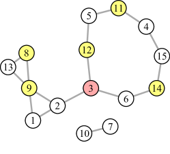
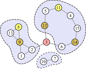
(a)	(b)

Figure 3: The graphical computation in Example 12 of the neighbourhood lattice $\mathfrak{T}_{j}(S)$ for $j=3$ and $S=\{9,8,11,12,14\}$. (a) Original graph $G$ with $j$ and $S$ specified with different colors. From this figure, it is easy to see that $S^{*}=\{9,12,14\}$ is the smallest subset of $S$ that separates $j$ from $S\setminus S^{*}$, hence $m_{j}(S)=S^{*}$. (b) Illustration of the three connected components which result after removing node $j=3$. As a result of Theorem 5, we can work in each component separately. For example, restricted to the left component $G_{1}=\{1,2,8,9,13\}$, the minimal subset of $S\cap G_{1}=\{8,9\}$ that separates $j=3$ from the rest of $S\cap G_{1}$ is $S^{*}_{1}=\{9\}$. Within $G_{1}$, $S^{*}_{1}$ separates $\{8,13\}$ from $j=3$. Hence, the restricted lattice $\mathfrak{T}_{j}(S\cap G_{1};G_{1})=[\{9\},\{9,8,13\}]$.

Example 12.

Continuing the previous examples, let $j=3$ and $S=\{9,8,11,12,14\}$. It is clear from Figure 3(a) that the smallest subset $S^{*}$ of $S$ separating $j$ from $S\setminus S^{*}$ is $\{9,12,14\}$. Hence, $m_{j}(S)=S^{*}$. Similarly, $E_{j}(S^{*})=\{4,5,7,8,10,11,13,15\}$ and $M_{j}(S)=S^{*}\cup E_{j}(S^{*})$. To verify Theorem 5, note that removing $j$ breaks $G$ into three connected components $G_{1}=\{1,2,8,9,13\}$, $G_{2}=\{7,10\}$ and $G_{3}=\{4,5,6,11,12,14,15\}$, as illustrated in Figure 3(b). Then we can compute the restricted lattices $\mathcal{T}_{j}(S\cap G_{k};G_{k}),k=1,2,3$. Using the notation $[m,M]$ to represent a lattice with minimum and maximum elements $m$ and $M$, respectively, the three lattices are: $[\{9\},\{8,9,13\}]$, $[\{12,14\},\{4,5,11,12,14,15\}]$ and $[\emptyset,\{7,10\}]$. It is clear that the minimal and maximal elements of the original lattice are the disjoint union of the corresponding elements of these three lattices.

Example 13.

Consider a Markov chain $X_{1}-X_{2}-\cdots-X_{d}$ with $V=[d]$. Define $j_{*}:=\sup\{\ell\in S:\ell<j\}$ and $j^{*}:=\inf\{\ell\in S:\ell>j\}$. Then we have for any $j$ and $S\subset V_{-j}$,

$$m(j;S) =\begin{cases}\{j_{*}\},&\{\ell\in S:\ell>j\}=\emptyset\\ \{j^{*}\},&\{\ell\in S:\ell<j\}=\emptyset\\ \{j^{*},j_{*}\},&\text{otherwise},\end{cases}$$

$$M(j;S) =\begin{cases}\{\ell\in V_{-j}:\ell<j_{*}\},&\{\ell\in S:\ell>j\}=\emptyset\\ \{\ell\in V_{-j}:\ell>j^{*}\},&\{\ell\in S:\ell<j\}=\emptyset\\ \{\ell\in V_{-j}:\ell>j_{*}\}\cup\{\ell\in V_{-j}:\ell<j^{*}\},&\text{otherwise}.\end{cases}$$

To verify Theorem 5, there are three cases: (i) $j=1$, (ii) $j=d$, and (iii) $1<j<d$. In (i) and (ii), removing $j$ results in a single connected component, corresponding to the first two cases above. In (iii), removing $j$ leaves two connected components, corresponding to the third case.

Example 14.

Recall Example 4, which describes a graphoid that is probabilistically representable but not representable as the separation graphoid of any undirected graph or directed acyclic graph. We can explicitly construct an example by considering $\nu=\mathcal{N}(0,\Sigma)$ where $\Sigma$ is defined by:

$$\Sigma^{-1}=\begin{pmatrix}3&1&1&0&0&0&0\\ 1&3&0&1&0&0&0\\ 1&0&3&1&0&0&0\\ 0&1&1&3&0&0&0\\ 0&0&0&0&4&3&-1\\ 0&0&0&0&3&5&-3\\ 0&0&0&0&-3&-3&3\\ \end{pmatrix}.$$

Consider the undirected graph $G=(V,E)$ given by the nonzero entries of $\Sigma^{-1}$. It is easy to verify that $X_{5}\mathchoice{\mathrel{\hbox to0.0pt{$\displaystyle\perp$\hss}\mkern 4.0mu{\displaystyle\perp}}}{\mathrel{\hbox to0.0pt{$\textstyle\perp$\hss}\mkern 4.0mu{\textstyle\perp}}}{\mathrel{\hbox to0.0pt{$\scriptstyle\perp$\hss}\mkern 4.0mu{\scriptstyle\perp}}}{\mathrel{\hbox to0.0pt{$\scriptscriptstyle\perp$\hss}\mkern 4.0mu{\scriptscriptstyle\perp}}}_{\!\!\!\nu}X_{6}$ but are not separated by the empty set (i.e. $(5,6)\in E$). That is, $(5,6,\emptyset)\in\mathcal{I}(\nu)$ but $(5,6,\emptyset)\notin\mathcal{I}(G)$. Thus $\mathcal{I}(G)\neq\mathcal{I}(\nu)$. Indeed, as described in Example 4, no undirected graph satisfies $\mathcal{I}(G)=\mathcal{I}(\nu)$. Nonetheless, the lattice construction still applies since $\mathcal{I}(\nu)$ is a Gaussoid. For example, suppose we wish to check the CI relation $X_{5}\mathchoice{\mathrel{\hbox to0.0pt{$\displaystyle\perp$\hss}\mkern 4.0mu{\displaystyle\perp}}}{\mathrel{\hbox to0.0pt{$\textstyle\perp$\hss}\mkern 4.0mu{\textstyle\perp}}}{\mathrel{\hbox to0.0pt{$\scriptstyle\perp$\hss}\mkern 4.0mu{\scriptstyle\perp}}}{\mathrel{\hbox to0.0pt{$\scriptscriptstyle\perp$\hss}\mkern 4.0mu{\scriptscriptstyle\perp}}}_{\!\!\!\nu}X_{6}$, which can be done via (9) with $j=5$, $i=6$, and $C=\emptyset$:

$$m(j;Ci)=m(5;\{6\})=\emptyset\subset C=\emptyset.$$

Since $\nu$ is a Gaussian, it is easy to verify that indeed $X_{5}\mathchoice{\mathrel{\hbox to0.0pt{$\displaystyle\perp$\hss}\mkern 4.0mu{\displaystyle\perp}}}{\mathrel{\hbox to0.0pt{$\textstyle\perp$\hss}\mkern 4.0mu{\textstyle\perp}}}{\mathrel{\hbox to0.0pt{$\scriptstyle\perp$\hss}\mkern 4.0mu{\scriptstyle\perp}}}{\mathrel{\hbox to0.0pt{$\scriptscriptstyle\perp$\hss}\mkern 4.0mu{\scriptscriptstyle\perp}}}_{\!\!\!\nu}X_{6}$.

7 Projection and regression interpretation

An alternative perspective on the neighbourhood lattice arises in the context of regression models in statistical applications. In particular, the notion of neighbourhood regression has played a prominent role in learning graphical models (e.g. [MB06, Rav+10, Yan+15]). This in turn bears a natural relation to orthogonal projections, which suggests a possible connection between the lattice of projections on a Hilbert space and the neighbourhood lattice. In this section, we explore these connections and illustrate the utility of the projection interpretation by providing an independent proof (based on abstract projection lattices) that partial orthogonality gives rise to a neighbourhood lattice.

7.1 The regression lattice

Let $X=(X_{j})_{j\in V}$ be a square-integrable random vector with covariance matrix $\Sigma=\operatorname{cov}(X)$ and joint distribution $\nu$. We view each $X_{j}$ as an element of the $L^{2}$ space of random variables. For any $S\subset V$, let $P_{S}$ denote the $L^{2}$ projection onto the span of $X_{S}=\{X_{i},\;i\in S\}$. For simplicity, we write $P_{j}=P_{\{j\}}$ to denote projection on the span of $\{X_{j}\}$, i.e., we drop the brackets for singleton sets. With some abuse of notation, let us also view $X$ as a set $X=\{X_{j},j\in V\}$ and recall the graphoid $\mathcal{I}(\operatorname{Proj}(X))$ defined by the partial orthogonality relation (1). Relative to $\mathcal{I}(\operatorname{Proj}(X))$, we have Markov boundaries $m(j;S)$ and the neighbourhood lattices $\mathfrak{T}_{j}(S)$ defined via (2) and (4), respectively. Throughout this section, in order to avoid ambiguity, we always explicitly reference the underlying graphoid, i.e. by writing $\mathfrak{T}_{j}(S;\nu):=\mathfrak{T}_{j}(S;\mathcal{I}(\nu))$ for the probabilistic graphoid induced by conditional independence and $\mathfrak{T}_{j}(S;\operatorname{Proj}(X)):=\mathfrak{T}_{j}(S;\mathcal{I}(\operatorname{Proj}(X)))$ for the projection graphoid induced by partial orthogonality (cf. (1)). Note that these are in general distinct.

The following, which we call the regression lattice, is closely related to the neighbourhood lattice $\mathfrak{T}_{j}(S;\operatorname{Proj}(X))$:

Definition 3 (Regression lattice).

For any $S\subset V_{-j}$, define a collection of subsets by

$$\mathcal{T}_{j}(S)=\{U\subset V_{-j}:\;P_{U}P_{j}=P_{S}P_{j}\}.$$ (18)

In other words, for any $j$, $\mathcal{T}_{j}(S)$ is the collection of subsets $U\subset V_{-j}$ such that the projection of $X_{j}$ onto $\{X_{i},\,i\in U\}$ is invariant. Note that $\mathcal{T}_{j}(S)$ is well-defined even when $\Sigma$ is rank-deficient.

The name “regression lattice” may seem peculiar by inspection of the definition alone. That $\mathcal{T}_{j}(S)$ is indeed a lattice will be established in Theorem 6 below. Let us first explain our use of the adjective “regression”: Let $\beta_{j}(S)$ be the coefficient vector obtained after regressing $X_{j}$ onto $X_{S}$, that is

$$\beta_{j}(S) :=\operatorname*{argmin}_{\beta\,\in\,\mathbb{R}^{d},\;\operatorname{supp}(\beta)\,\subset\,S}\mathbb{E}(X_{j}-\beta^{T}X)^{2},$$ (19)

where $\operatorname{supp}(a)=\{i:a_{i}\neq 0\}$ denotes the support of a vector $a$. Equivalently, $\beta_{j}(S)^{T}X$ is the orthogonal projection of $X_{j}$ onto $X_{S}$ in the space of square-integrable random variables. The coefficients in $\beta_{j}(S)$ are also known as the partial regression coefficients for the variable $j$ regressed on the variables $S$. We will often refer to them simply as regression coefficients. Then, assuming $\Sigma\succ 0$, we have:

$$\begin{split}\mathcal{T}_{j}(S)&=\{U\subset V_{-j}:\;\beta_{j}(U)=\beta_{j}(S)\}\\ &=\big{\{}U\subset V_{-j}:\;\operatorname{supp}(\beta_{j}(U))=\operatorname{supp}(\beta_{j}(S))\big{\}}.\end{split}$$ (20)

By definition, $\operatorname{supp}(\beta_{j}(S))\subset S$.

The next result shows that $\mathcal{T}_{j}(S)$ is in fact the same as the neighbourhood lattice induced by partial orthogonality with respect to the random vector $X$. As an immediate consequence, this also proves that $\mathcal{T}_{j}(S)$ is indeed a lattice.

Theorem 6.

Assume that $\Sigma:=\operatorname{cov}(X)\succ 0$. Then, we have

$$\mathcal{T}_{j}(S)=\mathfrak{T}_{j}(S;\operatorname{Proj}(X))$$ (21)

for all $j\in V$ and $S\subset V_{-j}$.

Combined with (20), Theorem 6 explains the name regression lattice. In the remainder of this section, we explore the properties of this lattice and its connection to the previously defined neighbourhood lattice.

Remark 3.

By definition, the regression lattice $\mathcal{T}_{j}(S)$ depends only on the random vector $X$, and is not defined relative to any underlying graphoid. Contrast this with the definition of the neighbourhood lattice, which explicitly requires an underlying compositional graphoid $\mathcal{I}$, which may or may be generated by the distribution of some random vector $X$. In particular, we stress that $\mathcal{T}_{j}(S)$ is not the same as $\mathfrak{T}_{j}(S;\nu)$. See also the discussion after Lemma 7 below.

7.2 Comparison of lattices

We have now defined two objects: The neighbourhood lattice and the regression lattice. Theorem 6 showed that the regression lattice is in fact the same as the neighbourhood lattice $\mathfrak{T}_{j}(S;\operatorname{Proj}(X))$ that arises from partial orthogonality, as defined in (1). In this section, we explore the relationship between the regression lattice and the neighbourhood lattice $\mathfrak{T}_{j}(S;\nu)$ that arises from conditional independence.

Consider the setting in which we have a random vector $X\in L^{2}$, so that both $\mathfrak{T}_{j}(S;\nu)$ and $\mathcal{T}_{j}(S)$ are well-defined lattices. The main result of this section shows that $\mathfrak{T}_{j}(S;\nu)$ is always a subset of $\mathcal{T}_{j}(S)$, and equality holds if $X$ is Gaussian.

Lemma 7.

Let $X=(X_{j})_{j\in V}\in L^{2}$ be a random vector. Then:

1. Without additional assumptions, $\mathfrak{T}_{j}(S;\nu)\subset\mathcal{T}_{j}(S)$.

2. If $X\sim\mathcal{N}(0,\Sigma)$ for some $\Sigma\succ 0$, then $\mathfrak{T}_{j}(S;\nu)=\mathcal{T}_{j}(S)$.

Thus, when $X\sim\mathcal{N}(0,\Sigma):=\nu$, we have

$$\mathfrak{T}_{j}(S;\nu)=\mathcal{T}_{j}(S)=\mathfrak{T}_{j}(S;\operatorname{Proj}(X)).$$ (22)

This is not true in general, however, since partial orthogonality is weaker than conditional independence.

To prove this result, we recall some important facts:

1. The regression coefficients are given by $\beta_{j}(S)=\Sigma_{S,S}^{-1}\Sigma_{S,j}$;

2. The projection lattice can be written as $\mathcal{T}_{j}(S)=\big{\{}U\subset V_{-j}:\;\operatorname{supp}(\beta_{j}(U))=\operatorname{supp}(\beta_{j}(S))\big{\}}$ (cf. (20));

3. If $X\sim\mathcal{N}(0,\Sigma)$ for some $\Sigma\succ 0$ then $X_{j}\mathchoice{\mathrel{\hbox to0.0pt{$\displaystyle\perp$\hss}\mkern 4.0mu{\displaystyle\perp}}}{\mathrel{\hbox to0.0pt{$\textstyle\perp$\hss}\mkern 4.0mu{\textstyle\perp}}}{\mathrel{\hbox to0.0pt{$\scriptstyle\perp$\hss}\mkern 4.0mu{\scriptstyle\perp}}}{\mathrel{\hbox to0.0pt{$\scriptscriptstyle\perp$\hss}\mkern 4.0mu{\scriptscriptstyle\perp}}}S-m\,\mid\,m$ for $m=\operatorname{supp}(\beta_{j}(S))$.

Proof of Lemma 7.

(a) This follows by direct calculation using (A1) and (20).

(b) Suppose $X\sim\mathcal{N}(0,\Sigma)$. Let $\mathcal{T}_{j}(S)=[m,M]$ and $U\in\mathcal{T}_{j}(S)$. Since $m=\operatorname{supp}(\beta_{j}(S))=\operatorname{supp}(\beta_{j}(U))$, (A3) implies $X_{j}\mathchoice{\mathrel{\hbox to0.0pt{$\displaystyle\perp$\hss}\mkern 4.0mu{\displaystyle\perp}}}{\mathrel{\hbox to0.0pt{$\textstyle\perp$\hss}\mkern 4.0mu{\textstyle\perp}}}{\mathrel{\hbox to0.0pt{$\scriptstyle\perp$\hss}\mkern 4.0mu{\scriptstyle\perp}}}{\mathrel{\hbox to0.0pt{$\scriptscriptstyle\perp$\hss}\mkern 4.0mu{\scriptscriptstyle\perp}}}S-m\,\mid\,m$, so that $m\in\mathfrak{T}_{j}(S;\nu)$. Similarly, $m\in\mathfrak{T}_{j}(U;\nu)$. Since these lattices are disjoint, it follows that $\mathfrak{T}_{j}(S;\nu)=\mathfrak{T}_{j}(U;\nu)$. But then $U\in\mathfrak{T}_{j}(S;\nu)$, as desired. ∎

7.3 Projection lattice approach

We now give an independent proof that $\mathcal{T}_{j}(S)$ is a convex lattice, using only the algebraic properties of projections. The proof reveals where the lattice structure of $\mathcal{T}_{j}(S)$ comes from: It is inherited from the natural lattice structure possessed by projections on a Hilbert space. We will assume that the reader is familiar with the basic theory of Hilbert spaces and their associated projection lattices; a detailed introduction to these topics can be found in [FW10, Bla06]. We provide a short overview in Section 7.3.1 below. This section can safely be skipped by the reader without interrupting the sequel.

7.3.1 Background on projection lattice

For a (separable) Hilbert space $\mathcal{H}$, let $B(\mathcal{H})$ be the space of bounded linear operators on $\mathcal{H}$. For an operator $P\in B(\mathcal{H})$, let $\operatorname{ran}(P):=P\mathcal{H}:=\{Px:\;x\in\mathcal{H}\}$ denote its range and $P^{*}$ its adjoint, defined via the relation $\langle x,P^{*}y\rangle=\langle Px,y\rangle$ for all $x,y\in\mathcal{H}$. An operator $P\in B(\mathcal{H})$ is an orthogonal projection if and only if it is self-adjoint and idempotent: $P^{*}=P=P^{2}$. The set of orthogonal projections in $B(\mathcal{H})$ is denoted as $\operatorname{Proj}(\mathcal{H})$. The range of any orthogonal projection is a closed linear subspace of $\mathcal{H}$. In fact, there is a bijection between $\operatorname{Proj}(\mathcal{H})$ and closed linear subspaces of $\mathcal{H}$. The latter can be ordered by inclusion, which induces a natural (partial) order on $\operatorname{Proj}(\mathcal{H})$ via the bijection. This order can be characterized as follows:

Lemma 8.

For $P,Q\in\operatorname{Proj}(\mathcal{H})$, the following are equivalent:

$$(a)\;P=PQ,\quad(b)\;P=QP,\quad(c)\;\operatorname{ran}(P)\subset\operatorname{ran}(Q).$$

When any of these conditions hold we write $P\leq Q$.

The equivalence of (a) and (b) follows from self-adjointness of orthogonal projections. Note that $PQ$ in Lemma 8 is not necessarily a projection (unless $P$ and $Q$ commute). One can show that the above order turns $\operatorname{Proj}(\mathcal{H})$ into a complete lattice. The join and meet of two elements $P,Q\in\operatorname{Proj}(\mathcal{H})$ can be expressed as follows:

$$P\wedge Q =\text{the projection onto $\operatorname{ran}(P)\cap\operatorname{ran}(Q)$}$$

$$P\vee Q =\text{the projection onto the closed linear span of $\operatorname{ran}(P)\cup\operatorname{ran}(Q)$.}$$

We also let $P^{\perp}:=I-P$, the orthogonal complement of $P$. Note that $P\vee P^{\perp}=I$ (the identity operator) and $P\wedge P^{\perp}=\{0\}$. Also, $P\leq Q$ iff $Q^{\perp}\leq P^{\perp}$. See for example [FW10, Section 5, p. 24 ] and [Bla06, Section II.3.2, p. 78 ] and the references therein.

7.3.2 Abstract lattice theorem

We now show that $\mathcal{T}_{j}(S)$ is a lattice isomorphic to an interval of the subset lattice, by combining two abstract results. Consider a Hilbert space $\mathcal{H}$ and a collection of vectors $\mathcal{X}=\{x_{j}\}_{j\in J}\subset\mathcal{H}$, not necessarily finite. The next result and its proof (except the convexity assertion) are due to Tristan Bice [Bic]:

Theorem 7.

For an operator $A\in B(\mathcal{H})$ and projection $P\in\operatorname{Proj}(\mathcal{H})$, define

$$\mathcal{Q}(A,P):=\{Q\in\operatorname{Proj}(\mathcal{H}):\,PA=QA\}.$$

Then $\mathcal{Q}(A,P)$ is a complete convex sublattice of $\operatorname{Proj}(\mathcal{H})$.

For any finite $S\subset\mathcal{X}$, let $P_{S}\in\operatorname{Proj}(\mathcal{H})$ be the projection onto the (closed) linear span of $S$. Recall that $\mathfrak{B}(\mathcal{X})$ is the complete lattice of all subsets of $\mathcal{X}$ ordered by inclusion. We also write $\mathfrak{B}_{\text{fin}}(\mathcal{X})$ for the lattice of all finite subsets of $\mathcal{X}$.

Proposition 2.

Assume that $\mathcal{X}\subset\mathcal{H}$ is a linearly independent set. Then,

$$\Pi(\mathcal{X}):=\{P_{S}:\;S\;\text{is a finite subset of}\;\mathcal{X}\}$$

is a sublattice of $\operatorname{Proj}(\mathcal{H})$ isomorphic to $\mathfrak{B}_{\text{fin}}(\mathcal{X})$.

The proposition implies that for any $S,T\subset\mathcal{X}$, we have $P_{S}\wedge P_{T}=P_{S\cap T}$ and $P_{S}\vee P_{T}=P_{S\cup T}$. Combining these two results, it follows that $\mathcal{T}_{j}(S)$ is lattice-isomorphic to an interval of the subset lattice since $\mathcal{T}_{j}(S)=\Pi(\{X_{i}\}_{i\in V_{-j}})\cap\mathcal{Q}(P_{X_{j}},P_{S})$.

Remark 4.

Proposition 2 and Theorem 7 apply to an infinite-dimensional Hilbert space $\mathcal{H}$ and infinitely many variables $\{X_{1},X_{2},\dots\}$. They also hold when the variables are dependent (i.e., $\Sigma$ is rank-deficient) if we remain at the level of projections (i.e., not map projections onto sets of variables).

8 Discussion

We have introduced the neighbourhood lattice for general compositional graphoids and its application to checking CI relations. Notably, this structure negates the need for a graphical representation of a graphoid, at the expense of requiring compositionality. We have shown that these lattices are efficiently computable, and have meaningful interpretations in special cases such as separation and projection graphoids. We also established a high-dimensional consistency result for Gaussian models, which we expect can be generalized to non-Gaussian settings using recent progress on nonparametric CI testing.

We conclude with some additional open questions. In Remark 2, we observed that many of the properties carry over even for non-compositional graphoids, however, a complete study of this more general case remains open. It would also be interesting to derive sharper upper bounds on the number of lattices in the lattice decomposition (Definition 2), as this has important computational implications (Section 4). It would also be interesting to explore consequences of the neighbourhood lattice for learning graphical models. In particular, since our results apply to any graphical model, this opens the door for learning more general (e.g. chain, mixed, etc.) graphical models without needing to assume faithfulness.

References

• [AAZ22] Arash Amini, Bryon Aragam and Qing Zhou “On perfectness in Gaussian graphical models” In International Conference on Artificial Intelligence and Statistics, 2022, pp. 7505–7517 PMLR
• [AC19] Mona Azadkia and Sourav Chatterjee “A simple measure of conditional dependence” In arXiv preprint arXiv:1910.12327, 2019
• [Ali+10] Constantin F Aliferis et al. “Local causal and Markov blanket induction for causal discovery and feature selection for classification Part I: Algorithms and empirical evaluation” In Journal of Machine Learning Research 11 JMLR. org, 2010, pp. 171–234
• [Ali+10a] Constantin F Aliferis et al. “Local causal and Markov blanket induction for causal discovery and feature selection for classification Part II: Analysis and extensions” In Journal of Machine Learning Research 11 JMLR. org, 2010, pp. 235–284
• [AP93] Steen Arne Andersson and Michael D Perlman “Lattice models for conditional independence in a multivariate normal distribution” In The Annals of Statistics JSTOR, 1993, pp. 1318–1358
• [ATS03] Constantin F Aliferis, Ioannis Tsamardinos and Alexander Statnikov “HITON: a novel Markov Blanket algorithm for optimal variable selection” In AMIA annual symposium proceedings 2003, 2003, pp. 21 American Medical Informatics Association
• [Bic] Tristan Bice “Collection of projection operators in finite dimension and algebraic techinques”, MathOverflow URL: http://mathoverflow.net/q/229239
• [BK19] Tobias Boege and Thomas Kahle “Construction methods for gaussoids” In arXiv preprint arXiv:1902.11260, 2019
• [Bla06] Bruce Blackadar “Operator Algebras” 122, Encyclopaedia of Mathematical Sciences Berlin, Heidelberg: Springer Berlin Heidelberg, 2006 DOI: 10.1007/3-540-28517-2
• [Bou+10] Remco Bouckaert, Raymond Hemmecke, Silvia Lindner and Milan Studeny “Efficient Algorithms for Conditional Independence Inference” In Journal of Machine Learning Research 11.112, 2010, pp. 3453–3479
• [Can+18] Clément L Canonne, Ilias Diakonikolas, Daniel M Kane and Alistair Stewart “Testing conditional independence of discrete distributions” In Proceedings of the 50th Annual ACM SIGACT Symposium on Theory of Computing, 2018, pp. 735–748
• [Daw01] A Philip Dawid “Separoids: A mathematical framework for conditional independence and irrelevance” In Annals of Mathematics and Artificial Intelligence 32.1-4 Springer, 2001, pp. 335–372
• [Daw79] A Philip Dawid “Conditional independence in statistical theory” In Journal of the Royal Statistical Society. Series B (Methodological) JSTOR, 1979, pp. 1–31
• [Daw80] A Philip Dawid “Conditional independence for statistical operations” In Annals of Statistics JSTOR, 1980, pp. 598–617
• [FW10] Ilijas Farah and Eric Wofsey “Set theory and operator algebras” In Appalachian Set Theory: 2006-2012, 2010, pp. 1–51
• [GBB18] Linda C. Gaag, Marco Baioletti and Janneke H. Bolt “A Lattice Representation of Independence Relations” In Proceedings of the Ninth International Conference on Probabilistic Graphical Models 72, Proceedings of Machine Learning Research Prague, Czech Republic: PMLR, 2018, pp. 487–498
• [GJ16] Tian Gao and Qiang Ji “Efficient Markov blanket discovery and its application” In IEEE transactions on Cybernetics 47.5 IEEE, 2016, pp. 1169–1179
• [GJ17] Tian Gao and Qiang Ji “Efficient score-based Markov blanket discovery” In International Journal of Approximate Reasoning 80 Elsevier, 2017, pp. 277–293
• [GP93] Dan Geiger and Judea Pearl “Logical and Algorithmic Properties of Conditional Independence and Graphical Models” In Ann. Statist. 21.4 The Institute of Mathematical Statistics, 1993, pp. 2001–2021 DOI: 10.1214/aos/1176349407
• [KB07] Markus Kalisch and Peter Bühlmann “Estimating High-Dimensional Directed Acyclic Graphs with the {PC}-Algorithm” In J. Mach. Learn. Res. 8 Cambridge, MA, USA: MIT Press, 2007, pp. 613–636
• [KF09] Daphne Koller and Nir Friedman “Probabilistic graphical models: principles and techniques” MIT press, 2009
• [Lau96] Steffen L Lauritzen “Graphical models” Oxford University Press, 1996
• [LM07] R Lněnička and F Matúš “On Gaussian condititional independence structures” In Kybernetika 43.3, 2007, pp. 327–342
• [LS18] Steffen Lauritzen and Kayvan Sadeghi “Unifying Markov properties for graphical models” In The Annals of Statistics 46.5 Institute of Mathematical Statistics, 2018, pp. 2251–2278
• [LS88] Steffen L Lauritzen and David J Spiegelhalter “Local computations with probabilities on graphical structures and their application to expert systems” In Journal of the Royal Statistical Society: Series B (Methodological) 50.2 Wiley Online Library, 1988, pp. 157–194
• [Mat93] František Matúš “PROBABILISTIC CONDITIONAL INDEPENDENCE STRUCTURES AND MATROID THEORY: BACKGROUND1” In International Journal Of General System 22.2 Taylor & Francis, 1993, pp. 185–196
• [Mat95] F. Matus “Conditional independences among four random variables II” Combinatorics, ProbabilityComputing, 1995
• [MB06] Nicolai Meinshausen and Peter Bühlmann “High-dimensional graphs and variable selection with the Lasso” In Annals of Statistics 34.3 Institute of Mathematical Statistics, 2006, pp. 1436–1462
• [MS95] F. Matus and Milan Studenỳ “Conditional independences among four random variables I” Combinatorics, ProbabilityComputing, 1995
• [MT99] Dimitris Margaritis and Sebastian Thrun “Bayesian network induction via local neighborhoods” In Proceedings of the 12th International Conference on Neural Information Processing Systems, 1999, pp. 505–511
• [NBW20] Matey Neykov, Sivaraman Balakrishnan and Larry Wasserman “Minimax Optimal Conditional Independence Testing” In arXiv preprint arXiv:2001.03039, 2020
• [Nie+13] Mathias Niepert, Marc Gyssens, Bassem Sayrafi and Dirk Van Gucht “On the conditional independence implication problem: A lattice-theoretic approach” In Artificial Intelligence 202 Elsevier, 2013, pp. 29–51
• [Pea09] Judea Pearl “Causality” Cambridge university press, 2009
• [Pea88] Judea Pearl “Probabilistic reasoning in intelligent systems: Networks of plausible inference” Morgan Kaufmann, 1988
• [PP85] Judea Pearl and Azaria Paz “Graphoids: A graph-based logic for reasoning about relevance relations” University of California (Los Angeles). Computer Science Department, 1985
• [PV87] Judea Pearl and Thomas Verma “The logic of representing dependencies by directed graphs” University of California (Los Angeles). Computer Science Department, 1987
• [Rav+10] Pradeep Ravikumar, Martin J Wainwright, John D Lafferty and Others “High-dimensional Ising model selection using $\ell_{1}$-regularized logistic regression” In The Annals of Statistics 38.3 Institute of Mathematical Statistics, 2010, pp. 1287–1319
• [Sad17] Kayvan Sadeghi “Faithfulness of probability distributions and graphs” In The Journal of Machine Learning Research 18.1 JMLR. org, 2017, pp. 5429–5457
• [SGS00] Peter Spirtes, Clark Glymour and Richard Scheines “Causation, prediction, and search” The MIT Press, 2000
• [SP18] Rajen D Shah and Jonas Peters “The Hardness of Conditional Independence Testing and the Generalised Covariance Measure” In arXiv preprint arXiv:1804.07203, 2018
• [Sta+13] Alexander Statnikov, Nikita I Lytkin, Jan Lemeire and Constantin F Aliferis “Algorithms for discovery of multiple Markov boundaries” In Journal of Machine Learning Research 14.Feb, 2013, pp. 499–566
• [Sta97] Richard P Stanley “Enumerative Combinatorics (Volume 1)” In Cambridge studies in advanced mathematics, 1997
• [Stu06] Milan Studeny “Probabilistic conditional independence structures” Springer Science & Business Media, 2006
• [Stu15] Milan Studenỳ “How matroids occur in the context of learning Bayesian network structure.” In UAI, 2015, pp. 832–841
• [Stu89] Milan Studený “Multiinformation and the problem of characterization of conditional independence relations” In Problems of Control and Information Theory 18.1, 1989, pp. 3–16
• [Stu90] Milan Studeny “Conditional independence relations have no finite complete characterization” Citeseer, 1990
• [STU95] MILAN STUDENÝ “DESCRIPTION OF STRUCTURES OF STOCHASTIC CONDITIONAL INDEPENDENCE BY MEANS OF FACES AND IMSETS 1st part: introduction and basic concepts” In International Journal of General Systems 23.2 Taylor & Francis, 1995, pp. 123–137
• [Sul09] Seth Sullivant “Gaussian conditional independence relations have no finite complete characterization” In Journal of Pure and Applied Algebra 213.8 Elsevier, 2009, pp. 1502–1506
• [TPP98] Jin Tian, Azaria Paz and Judea Pearl “Finding minimal d-separators” Citeseer, 1998
• [Tsa+03] Ioannis Tsamardinos, Constantin F Aliferis, Alexander R Statnikov and Er Statnikov “Algorithms for Large Scale Markov Blanket Discovery” In FLAIRS conference 2, 2003, pp. 376–380
• [Whi35] Hassler Whitney “On the Abstract Properties of Linear Dependence” In American Journal of Mathematics 57.3 JSTOR, 1935, pp. 509–533
• [WJ08] Martin J Wainwright and Michael Irwin Jordan “Graphical models, exponential families, and variational inference” Now Publishers Inc, 2008
• [WW20] Yue Wang and Linbo Wang “Causal inference in degenerate systems: An impossibility result” 108, Proceedings of Machine Learning Research Online: PMLR, 2020, pp. 3383–3392
• [Yan+15] Eunho Yang, Pradeep Ravikumar, Genevera I Allen and Zhandong Liu “Graphical models via univariate exponential family distributions” In Journal of Machine Learning Research 16, 2015, pp. 3813–3847
• [ZL20] Benito Zander and Maciej Liśkiewicz “Finding minimal d-separators in linear time and applications” In Uncertainty in Artificial Intelligence, 2020, pp. 637–647 PMLR