tBDFS: Temporal Graph Neural Network Leveraging DFS

Abstract

Temporal graph neural networks (temporal GNNs) have been widely researched, reaching state-of-the-art results on multiple prediction tasks. A common approach employed by most previous works is to apply a layer that aggregates information from the historical neighbors of a node. Taking a different research direction, in this work, we propose tBDFS – a novel temporal GNN architecture. tBDFS applies a layer that efficiently aggregates information from temporal paths to a given (target) node in the graph. For each given node, the aggregation is applied in two stages: (1) A single representation is learned for each temporal path ending in that node, and (2) all path representations are aggregated into a final node representation. Overall, our goal is not to add new information to a node, but rather observe the same exact information in a new perspective. This allows our model to directly observe patterns that are path-oriented rather than neighborhood-oriented. This can be thought as a Depth-First Search (DFS) traversal over the temporal graph, compared to the popular Breath-First Search (BFS) traversal that is applied in previous works. We evaluate tBDFS over multiple link prediction tasks and show its favorable performance compared to state-of-the-art baselines. To the best of our knowledge, we are the first to apply a temporal-DFS neural network.

1 Introduction

Graphs are ubiquitous, and nowadays, many data sources spanning over diverse domains such as the Web, cybersecurity, economics, biology, and others are being modeled as a graph. Modeling a data source as a graph allows to detect rich structural patterns which are useful for a large variety of machine learning tasks, such as link-prediction and node classification (Cai, Zheng, and Chang 2018). Learning on graphs is challenging, with an handful of different approaches that have been proposed over the recent years. Among others, Graph Neural Networks (GNNs) have demonstrated state-of-the-art results over many different datasets and tasks (Kipf and Welling 2017; Hamilton, Ying, and Leskovec 2017; Veličković et al. 2017). GNNs allow to learn rich node (and edge) representations by applying neural network layers on the graph’s structure such as convolution (CNNs) or recurrent (RNNs) neural networks (Wu et al. 2020).

While learning over graphs has been widely researched, many aspects still remain a challenge. Such aspects include, among others, scaling learning models to large graphs, extracting meaningful features from the graph’s complex structure; and the focus of our work: handling temporal graphs. A temporal graph captures the evolution of networks over time, associating each edge between any two nodes in the graph with a timestamp. Using temporal GNNs, learning on the graph occurs over time, by applying the neural network layers according to the timeline in which the graph’s topology has evolved (Skardinga, Gabrys, and Musial 2021).

Most existing GNNs (Kipf and Welling 2017; Hamilton, Ying, and Leskovec 2017; Veličković et al. 2017), and specifically temporal GNNs (da Xu et al. 2020), extract features from the graph structure by following a rule with the following question in mind: “What have your neighbors been telling you?”. Practically, this rule is implemented by aggregating for each node in the graph the information from its neighbors. This aggregation is differential, making it a general layer that can be connected to any desired deep-learning architecture, such as stacking it one over the other. While stacking the GNN layers enlarges the receptive field of a node to nodes further in the graph, it still follows the above rule, making it hard to find patterns that may follow other rules.

In this work, we take a novel perspective, by exploring a different rule over temporal graphs, which aims to answer the following question: “Tell me how did you receive this information?”. Intuitively, while previous GNNs observe the graph in a Breadth-First manner (i.e., observing neighbors at each layer), we present an algorithm that also observes the graph in a Depth-First manner (i.e., observing paths at each layer). While there are previous GNN works (Yang et al. 2019; Chen et al. 2021; Lin et al. 2021; Ying et al. 2021) that recognize the importance of observing a path in the graph (and specifically in a DFS manner), they do not leverage the rich information of the path, nor can be trivially extended to temporal graphs. We hypothesize that, some tasks and datasets on temporal graphs hold patterns that are more DFS oriented rather than BFS oriented. Traversing the graph in a DFS manner allows to capture the effective order in which information flows in the network from a source to its target. This is in comparison to a BFS traversal, which always assumes that information flows from the neighborhood first, which is not always true; For example, it might be possible in some cases that, a node along a path to the target may have multiple unrelated neighbors, and hence, may add an undesired noise to the target node’s representation.

Figure 1 further illustrates an example of a task with a DFS pattern. We notice that, while a BFS approach is challenged with the extraction of the signal (as the information should correctly propagate through 3 hops), a DFS approach is able to extract the signal directly from the path without requiring any information propagation. As a more concrete example, let us consider the Booking dataset, which is one of the datasets being studied in our work. Lets assume that the event of a user’s visit to a city is represented by a temporal edge in the graph. If that same city was already visited in the past by the same user (i.e., user-city-user), a BFS approach would have to propagate the previous user node to the next user node via the intermediate city node. When propagating to an intermediate node, the propagation is shared across all its neighbors, meaning that it will be hard for the BFS approach to “remember” the relevant neighbor out of all the given neighbors. This issue gets even worse when the path is longer, as the information exponentially vanishes the larger the path is and the more neighbors they are. By utilizing the DFS approach, the path of user-city-user is given explicitly to the model, without being required to propagate the user through the city.

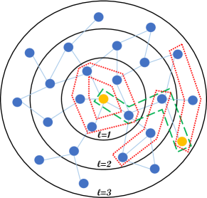
Figure 1: An illustration of how a given node (center) may depend on a distant node (bottom right). A BFS-oriented GNN is required to correctly propagate the information from the distant node through three other nodes, while also observing the “unrelated” neighbors (red-dotted area). Our DFS-oriented GNN captures the pattern directly via the path to that node (green dashed area).

Our DFS representation of a node is learned by two consecutive components: (1) Given a temporal path (as information travels in a “chronological” order in time) from a source node to a desired target node, the first component learns a path representation that is aware of all the nodes, edges, features and timestamps along that path. (2) Given the representations of all the temporal paths to a given target node from the previous component, the second component is responsible for aggregating all the paths into a final node representation.

It is important to note that, the DFS representation is presented with the exact same information as the BFS representation, with the only difference being in the way it is presented to the network. While previous works have enlarged the receptive field (which resulted with more information that is fed to the network), we demonstrate that, even without enlarging the receptive field, the same exact information can be fed to the network in a DFS way, enabling it to easily extract DFS patterns. Furthermore, we propose an efficient way to learn the DFS representation during the BFS learning phase.

Overall, we propose tBDFS – a temporal GNN architecture that given a node and a time, learns a DFS-aware representation of the node for that specific time. In order to combine between a BFS representation (using previous works (da Xu et al. 2020)) and our proposed DFS representation, we suggest learning the balance between the two representations, resulting in a final node representation that is aware of both types. We empirically evaluate tBDFS on a variety of link-prediction tasks using several real-world datasets, demonstrating its superior performance over competitive baselines.

2 Related Work

We review related works along two main dimensions which are the most relevant to ours: learning over temporal graphs and works that have leveraged paths or DFS.

2.1 Learning over Graphs

The field of learning on graphs has been studied for many years, but has grown widely in the last few years. Approaches over the years can be viewed along three “generarions”: matrix factorization, random walks, and graph neural networks.

The first generation included different factorization methods over the graph adjacency matrix. These works obtain node representations by preforming a dimensionality reduction over the adjacency matrix. This can be performed by learning to reconstruct the edges (Belkin and Niyogi 2001; Yan et al. 2006), the neighbors (Roweis and Saul 2000), or even the entire k-hop neighbors (Cao, Lu, and Xu 2015; Tenenbaum, De Silva, and Langford 2000).

The second generation proposed random walks over the graph in order to create a corpus representing the graph structure. For instance, DeepWalk (Perozzi, Al-Rfou, and Skiena 2014) represents the nodes as words and random walks as sentences, thereby reducing the problem to Word2Vec (Mikolov et al. 2013). Node2Vec (Grover and Leskovec 2016) extended this work by enabling a flexible neighborhood sampling strategy, which allows to smoothly interpolate between BFS and DFS.

The most recent generation of methods considers graph neural networks (GNN), which introduce generic layers that can be added to any desired deep learning architecture. For example, GCN (Kipf and Welling 2017) and GraphSAGE (Hamilton, Ying, and Leskovec 2017) presented a convolutional layer that computes the average neighbor representation. Graph attention networks (GAT) (Veličković et al. 2017) present an attention-based technique that learns the importance of each neighbor to the central node. (Ying et al. 2018) introduces a dedicated pooling mechanism for graphs that learns the soft clusters that should be pooled together. (Schlichtkrull et al. 2018) introduced a method that can handle different types of relation edges. Many works have demonstrated the superiority of GNNs over different tasks, such as molecules property prediction (Gilmer et al. 2017), protein-protein interaction prediction (Singer, Radinsky, and Horvitz 2020), fair job prediction (Singer and Kira 2022), human movement (Jain et al. 2016; Yan, Xiong, and Lin 2018; Feng et al. 2018), traffic forecasting (Yu, Yin, and Zhu 2018; Cui et al. 2018) and other urban dynamics (Wang and Li 2017). While GNNs are used as a layer that can be added to any architecture, some works proposed self-supervised techniques for learning node representations that can reconstruct the graph structure (Kipf and Welling 2016).

2.2 Learning over Temporal Graphs

Learning over temporal graphs (or dynamic networks) was widely studied in recent years. Earlier works applied matrix factorization or other types of aggregations over the temporal dimension (Dunlavy, Kolda, and Acar 2011; Yu, Aggarwal, and Wang 2017). Others (Nguyen et al. 2018) learned continuous dynamic embeddings using random walks that follow “chronological” paths that could only move forward in time. Such a time-sensitive random-walk has been shown to outperform static baselines (e.g., node2vec (Grover and Leskovec 2016)). More recent works utilized deep neural-networks. Among these works, (Singer, Guy, and Radinsky 2019) learned static representations for each graph snapshot and proposed an alignment method over the different snapshots. The final node representations were then obtained by using an LSTM layer that learns the evolution of each node over time. GNNs over temporal graphs was proposed in TGAT (da Xu et al. 2020), which extends GAT (Veličković et al. 2017) using the temporal dimension when aggregating the neighbors. For a given node, TGAT observes its neighbors as a sequence ordered by time of appearance. It then applies an attention layer that aggregates the information with temporal-awareness using a time encoder. Our tBDFS method extends over TGAT by adding a new layer that is responsible to capture DFS patterns in a temporal graph.

2.3 DFS in Graphs

Common to most previously studied methods (both over static and temporal graphs) is that each layer learns to aggregate the neighbors of a target node (i.e., in a BFS manner). Compared to that, in this work, we take a different approach and propose a temporal GNN that aggregates information in a DFS manner along paths that end at the target node.

Several previous works have further leveraged the “DFS view” of the graph. Among these works, (Grover and Leskovec 2016) have suggsted a random-walk approach with a flexible neighborhood sampling strategy between BFS and DFS exploration. However, their method does not handle node and edge features, nor can it be treated as a general differential layer. (Liu et al. 2019) have proposed to add a memory gate between the GNN layers, enabling to better remember how information has arrived to the target node. Yet, their method does not observe the DFS patterns, making it hard to extract specific paths that are important. (Lin et al. 2021) have proposed a method for learning over heterogeneous graphs using metapaths. Given a metapath, instances of it are sampled, while first-order nodes are aggregated separately from the higher-order ones. Therefore, their method as well does not actually leverage the DFS paths, but rather only perform aggregation of neighbors. (Yang et al. 2019) have further utilized a higher-order neighborhood by sampling nodes with shortest paths. These nodes were expected to be more relevant to the target node. Overall, none of the aforementioned works has actually leveraged the pattern of the path, nor handled temporal edges. (Chen et al. 2021) also proposed to aggregate information from higher-order nodes. To this end, for each node, a representation was first learned using a GNN. Then, random paths were sampled, where the importance of the last node of each path to the target node was learned via an LSTM model. The final representation was obtained as the weighted sum of all the last nodes. However, this method did not leverage actual information from the path, but rather has only learned its weight. Finally, (Ying et al. 2021) have proposed to leverage the entire graph structure during the GNN aggregation, while weighting the importance of two nodes by their shortest path. Yet, as the authors testify, their approach could only handle very small graphs with few nodes, which does not scale well.

2.4 Main Differences

Our work differs from previous works in several ways. Firstly, we generalize to temporal graphs which enables us to learn how information dynamically travels in the graph. Secondly, given a path, we learn both the importance of each of its nodes to its own representation; and the importance of each path to the target node representation. Thirdly, we leverage node features, edge features, and timestamps. Fourthly, we demonstrate the performance of the DFS aggregation on the exact same receptive field as the BFS aggregation. Differently from previous works, we show how actual DFS aggregation boosts performance, and not larger receptive fields. Furthermore, we sample the DFS paths recursively during the BFS aggregations, making it more efficient.

3 tBDFS Architecture

In this section we present the main building blocks that allow to learn both BFS and DFS patterns in a temporal graph. We start with basic temporal graph notations. We then shortly describe BFS graph attention and then present our proposed alternative of DFS graph attention. Our tBDFS approach is derived by combining both attention types.

Let $G=(V,E)$ now formally denote a temporal graph with nodes-set $V$ and edges-set $E$, respectively. We denote $(i,j)_{t}\in E$ as an undirected temporal edge, where node $i$ connects with a node $j$ at timestamp $t$. We denote $x_{i}\in{\mathbb{R}}^{d}$ the features of node $i\in V$, where $d$ is the number of features in the dataset. We further denote $x_{i,j}(t)\in{\mathbb{R}}^{d}$ the features of edge $(i,j)_{t}\in E$. For a given prediction task defined by a given loss function, our goal now is to find for each node $i\in V$ and timestamp $t$ a feature-vector (representation) $h_{i}(t)\in{\mathbb{R}}^{d}$ that minimizes the loss.

3.1 Functional Time Encoding

When using sequences in attention mechanisms, it is common to use positional encoding to allow the model to know the positions of the elements of the sequence (Kenton and Toutanova 2019). A problem raises when the sequence is continues rather than equally quantized (such as continues time series). In this case, positional encoding lacks to hold the continues information of the sequence. Therefore, an appropriate encoder is required. Instead of using positional embedding, we follow (da Xu et al. 2020) and leverage a continues time encoder $\Phi:T\rightarrow R^{d}$ from the time domain to a d-dimensional vector space:

$$\begin{split}\Phi(t)=\sqrt{\frac{1}{d}}\big{[}cos(w_{1}t),sin(w_{1}t),\dots,\\ cos(w_{d}t),sin(w_{d}t)\big{]}\end{split}$$ (1)

where $w_{1},..w_{d}$ are trainable parameters of the model. This encoder holds special properties following Bochner’s Theorem (Loomis 2013). We refer the reader to (da Xu et al. 2020) for additional details.

3.2 BFS Graph Attention

A common approach for learning temporal node representations $h_{i}(t)$, is to introduce a layer within a GNN setting that aggregates for each node the information from all its neighbors (Kipf and Welling 2017; Hamilton, Ying, and Leskovec 2017; Veličković et al. 2017). This can be thought of as a BFS aggregation, observing information in a Breadth-First manner.

Following (da Xu et al. 2020), given a timestamp $t$ and a node $i\in V$, with an initial feature vector $h^{(0)}_{i}=x_{i}$, a graph attention layer (at layer $l$) is used to update the node’s features $h^{(l)}_{i}$ according to its neighborhood. To this end, we first mask out neighbors in the future (where $t_{j}$ denotes the timestamp in which an edge $(i,j)$ has been formed):

$$\begin{split}\mathcal{N}_{i}(t)=\{j|(i,j)_{t_{j}}\in E\wedge t_{j}<t\}\end{split}$$ (2)

We notice that, the same neighbor may appear twice in the past. Therefore, we refer to a specific appearance in time as a “temporal neighbor”. For each temporal neighbor $j\in\mathcal{N}_{i}(t)$ that interacted with $i$ at timestamp $t_{j}<t$, we extract a feature representation that includes the neighbor’s own embedding, the edge features, and a time difference embedding:

$$\begin{split}h^{\prime(l-1)}_{j}=h^{(l-1)}_{j}(t_{j})\|x_{i,j}(t_{j})\|\Phi(\Delta t),\end{split}$$ (3)

where $\Delta t=t-t_{j}$, $\Phi$ is a time encoder as presented in Eq. 1, which embeds a time difference into a feature vector of size $d$, and $\|$ is the concatenation operator. Similarly, for the target node $i$, we apply the same logic:

$$\begin{split}h^{\prime(l-1)}_{i}=h^{(l-1)}_{i}(t)\|\bar{0}\|\Phi(\Delta t),\end{split}$$ (4)

where $\bar{0}\in{\mathbb{R}}^{d}$ is zero padding, as there is no actual edge between the target node to itself. Following (da Xu et al. 2020), we then apply a multihead cross-attention as follows:

$$\begin{split}\alpha^{m,(l)}_{ij}=\frac{exp(\mathbf{W}^{m,(l)}_{Q}h^{\prime(l-1)}_{i}\cdot\mathbf{W}^{m,(l)}_{K}h^{\prime(l-1)}_{j})}{\sum_{j\in\mathcal{N}_{i}(t)}{exp(\mathbf{W}^{m,(l)}_{Q}h^{(l-1)}_{i}\cdot\mathbf{W}^{m,(l)}_{K}h^{(l-1)}_{j})}},\\ h^{\prime(l)}_{i}(t)={\Big{\|}}^{M}_{m=1}\left(\sum_{j\in\mathcal{N}_{i}}{\alpha^{m,(l)}_{ij}\mathbf{W}^{m,(l)}_{V}h^{(l-1)}_{j}}\right),\\ h^{(l)}_{i}(t)=FFN(h^{(l-1)}_{i}(t)\|h^{\prime(l)}_{i}(t)),\end{split}$$ (5)

where $\mathbf{W}^{m,(l)}_{Q}$, $\mathbf{W}^{m,(l)}_{K}$, $\mathbf{W}^{m,(l)}_{V}\in{\mathbb{R}}^{3d\times 3d}$ are trainable parameters of the model, $M$ is the number of attention heads, and $FFN$ is a feed-forward neural-network.

Stacking multiple GNN layers one over the other allows to enlarge the receptive field of the node. Let the number of stacked layers be $L$. The final node representation is then:

$$h^{BFS}_{i}(t)=h^{(L)}_{i}(t)$$

3.3 DFS Graph Attention

While the receptive field of a given node grows with more layers, the information is being propagated in a BFS way, where information is being aggregated by observing the node’s neighbors (see Figure 1). Yet, by aggregating in such a manner, it is hard to extract information from a specific path. We therefore propose to learn an additional representation, $h^{DFS}_{i}(t)$, that observes the same receptive field as $h^{BFS}_{i}(t)$, but in a Depth-First manner.

Given a target node (as illustrated in the center of Figure 1), stacking $L$ GNN layers provides us with a $L$-hop neighborhood that effects the BFS representation. A different way of observing this exact same neighborhood, would be by extracting all the paths of length $L$ ending at the target node. Let $\mathcal{P}^{L}_{i}(t)$ represent the group of all temporal paths of length $L$ ending at node $i$ at timestamp $t$. A specific path, $p_{r}=(j_{0},j_{1},...,j_{L})\in\mathcal{P}^{L}_{i}(t)$, holds a list of all nodes in the path (ordered from the latest to the earliest in time), where $j_{0}=i$, and $j_{L}$ is the last (source) node in the path. As we want to propagate the information in a Depth-First way, we observe each path separately. In order to do so, we aggregate the nodes in the path $p_{r}$ into a single representation. We next note that, such a path may be thought as a sequence of edge formation events over time. In this work, we have chosen to leverage the attention mechanism as it demonstrated state-of-the-art results over sequential data aggregation, as follows:

$$\begin{split}\alpha^{m,(l)}_{ij}=\frac{exp(\mathbf{W}^{m,(l)}_{Q}h^{\prime(l-1)}_{i}\cdot\mathbf{W}^{m,(l)}_{K}h^{\prime(l-1)}_{j})}{\sum_{j\in p_{r}}{exp(\mathbf{W}^{m,(l)}_{Q}h^{(l-1)}_{i}\cdot\mathbf{W}^{m,(l)}_{K}h^{(l-1)}_{j})}}\\ h^{\prime(l)}_{i,r}(t)={\Big{\|}}^{M}_{m=1}\left(\sum_{j\in p_{r}}{\alpha^{m,(l)}_{ij}\mathbf{W}^{m,(l)}_{V}h^{(l-1)}_{j}}\right)\\ h^{(l)}_{i,r}(t)=FFN(h^{(l-1)}_{i,r}(t)\|h^{\prime(l)}_{i}(t))\end{split}$$ (6)

where $\mathbf{W}^{m,(l)}_{Q}$, $\mathbf{W}^{m,(l)}_{K}$, $\mathbf{W}^{m,(l)}_{V}\in{\mathbb{R}}^{3d\times 3d}$ are trainable parameters of the model, $M$ is the number of attention heads, and $FFN$ is a feed-forward neural network. We can notice that Eq. 6 is quite similar to Eq. 5. This is not by accident, as the latter performs a BFS aggregation of the neighbors, while the former performs a DFS aggregation over the path nodes. Overall, there are three main differences between the two: (1) The aggregation in Eq. 6 is over nodes in a specific path, while in Eq. 5 it is over neighbors of a specific node. (2) While BFS uses the time difference of a node from its parent, DFS uses the time difference of each node in the path from the target node. (3) The aggregation is per a single path of the target node. That actually means that, in order to obtain the target node’s final representation, we still need to combine the representation of all its associated paths.

At this point, for each node $i\in{V}$, we hold a representation for each of its possible paths, where $i$ acts as the path target. Therefore, in order to obtain a single representation for node $i$, we further aggregate all its path representations, as follows:

$$\begin{split}h^{(l)}_{i}(t)=Aggregate(\{h^{(l)}_{i,r}(t)|p_{r}\in\mathcal{P}^{L}_{i}(t)\}),\end{split}$$ (7)

where the $Aggregate$ function can be any aggregation such as average or attention. In this work, we have chosen to leverage the multi-head attention mechanism (Vaswani et al. 2017); where for each node $i$, we treat $h^{BFS}_{i}(t)$ as the query, and $\{h^{(l)}_{i,r}(t)|p_{r}\in\mathcal{P}^{L}_{i}(t)\}$ as both the keys and values.

It is important to note that, for a receptive field of $L$-hops, the BFS method proposed in Section 3.2 is required to learn a different attention layer for each hop (i.e., an attention layer for each GNN layer). Compared to that, our method requires only two layers for any given receptive field: one layer for aggregating the path into a single representation, and the second for aggregating all paths into a final node representation. This means that, we can define $h^{DFS}_{i}(t)=h^{(1)}_{i}(t)$ after only one layer, without having to stack layers in order to capture information from the desired receptive field.

3.4 tBDFS: Balancing BFS and DFS

As the trade-off between BFS and DFS may vary among graphs in the real world, we apply a final aggregation over the two representations (deriving our overall tBDFS approach):

$$h^{\prime}_{i}(t)=\alpha\cdot h^{BFS}_{i}(t)\\ +(1-\alpha)\cdot h^{DFS}_{i}(t),$$ (8)

where $\alpha\in[0,1]$ is a hyper-parameter that is responsible of balancing and smoothly interpolating between BFS and DFS.

3.5 Efficient Path Sampling

Extracting $\mathcal{P}^{L}_{i}(t)$ in a brute-force way can be very time consuming. As we need to also calculate the BFS representations (see Eq. 8), we further propose a way to capture the temporal paths during the BFS implementation, making it more efficient. Since the BFS implementation is recursive (each layer is a deeper call that “explodes” the new neighbors), in every recursive call, we explode the current path up to node $i$ with its temporal neighbors, $\mathcal{N}_{i}(t)$, into $|\mathcal{N}_{i}(t)|$ new paths (that will continue to explode in the next recursive calls). When the recursive call reaches its final depth ($L$), we notice that the group of exploded paths is equal to $\mathcal{P}^{L}_{i}(t)$. This is done without any additional computation over the BFS method. Next, all is left to do is to propagate the paths back to the initial call and run Eq. 6 and Eq. 7 on the paths in $\mathcal{P}^{L}_{i}(t)$. This, therefore, not just resolves us with the DFS node representation, but also promises that the DFS aggregation is presented with the exact same information as the BFS aggregation.

4 Evaluation

Table 1: Main results. Boldfaced results indicate a statistically significant difference.

Model		Reddit			Booking			Act-mooc			Movielens			Wikipedia
		Accuracy	F1		Accuracy	F1		Accuracy	F1		Accuracy	F1		Accuracy	F1
Temporal	tBDFS	$\mathbf{68.70(\pm 0.36)}$	$\mathbf{74.04(\pm 0.25)}$		$\mathbf{74.71(\pm 0.51)}$	$\mathbf{78.84(\pm 0.52)}$		$\mathbf{56.45(\pm 0.30)}$	$69.15(\pm 0.10)$		$\mathbf{72.94(\pm 0.09)}$	$72.76(\pm 0.59)$		$\mathbf{86.99(\pm 0.15)}$	$\mathbf{87.32(\pm 0.16)}$
	TGAT	$66.26(\pm 0.13)$	$72.23(\pm 0.11)$		$73.24(\pm 0.29)$	$78.06(\pm 0.28)$		$55.92(\pm 0.03)$	$69.08(\pm 0.17)$		$72.65(\pm 0.06)$	$72.84(\pm 0.50)$		$86.79(\pm 0.05)$	$87.03(\pm 0.06)$
	tNodeEmbed	$67.67(\pm 0.89)$	$68.59(\pm 0.46)$		$58.85(\pm 0.49)$	$55.80(\pm 0.80)$		$54.66(\pm 0.66)$	$54.43(\pm 1.30)$		$55.68(\pm 1.06)$	$38.88(\pm 4.01)$		$67.32(\pm 0.52)$	$67.44(\pm 0.31)$
	GAT+T	$65.31(\pm 0.55)$	$73.22(\pm 0.33)$		$62.56(\pm 0.27)$	$65.00(\pm 0.45)$		$52.23(\pm 0.58)$	$66.48(\pm 0.52)$		$57.25(\pm 0.90)$	$61.32(\pm 0.77)$		$76.0(\pm 0.59)$	$79.52(\pm 0.40)$
Static	VGAE	$65.47(\pm 0.23)$	$72.35(\pm 0.13)$		$60.40(\pm 0.32)$	$62.22(\pm 0.57)$		$52.15(\pm 0.20)$	$66.55(\pm 0.09)$		$56.90(\pm 0.31)$	$62.68(\pm 0.11)$		$72.69(\pm 0.17)$	$77.64(\pm 0.15)$
	GAE	$66.24(\pm 0.17)$	$72.75(\pm 0.10)$		$61.31(\pm 0.14)$	$62.63(\pm 0.18)$		$51.00(\pm 0.48)$	$66.57(\pm 0.10)$		$56.93(\pm 0.24)$	$62.67(\pm 0.35)$		$73.32(\pm 0.11)$	$77.94(\pm 0.10)$
	node2vec	$59.85(\pm 0.03)$	$70.37(\pm 0.03)$		$60.94(\pm 0.13)$	$64.69(\pm 0.18)$		$49.47(\pm 0.23)$	$57.49(\pm 0.18)$		$51.94(\pm 0.13)$	$54.82(\pm 0.23)$		$69.85(\pm 0.30)$	$75.06(\pm 0.27)$

As a concrete task for evaluating tBDFS, we now apply it on the link-prediction task over a variety of temporal graph datasets. We first describe the datasets and our experimental setup (model implementation and training, baselines and metrics). We then present the evaluation results.

4.1 Datasets

The following datasets were used in our evaluation:

• Wikipedia (Kumar, Zhang, and Leskovec 2019): A bipartite graph representing users editing Wikipedia pages. Each edge represents an edit event with its timestamp.

• Reddit (Kumar et al. 2018): A graph representing links between subreddits in the Reddit website. A link occurs when a post in one subreddit is created with a hyperlink to a post in a second subreddit.

• Act-mooc (Kumar, Zhang, and Leskovec 2019): A bipartite graph representing students taking courses. Each edge is represented with a timestamp of when the student took the course.

• MovieLens (Harper and Konstan 2015): A bipartite graph representing $1$ million users’ movie ratings. Each edge represents a rating event with its timestamp.

• Booking (Goldenberg et al. 2021): A bipartite graph used in the WSDM2021 challenge. A temporal edge represents a user visiting a city at a given time.

We split each dataset over time, with $70\%$ of the edges used for training, $15\%$ used for validation, and the rest (most recent) $15\%$ for testing.

4.2 Experimental Setup

Model implementation and training

We implement tBDFS with pytorch (Paszke et al. 2017). We use the Adam (Kingma and Ba 2015) optimizer, with a learning rate of $10^{-4}$, $\beta_{1}=0.9$, $\beta_{2}=0.999$, $\ell_{2}$, dropout $p=0.1$ and batch size of $200$. For a fair comparison, following (Kipf and Welling 2017), for all GNN baselines (including tBDFS), we set the number of layers $L=2$.

During training, for each temporal edge $(i,j)_{t}$, we sample a negative edge $(i,j^{\prime})_{t}$, and learn to contrast between the two, following the loss proposed in (da Xu et al. 2020):

$$\begin{split}Loss=-\sum_{i}\big{[}log(\sigma(FFN(h^{\prime}_{i}(t)\|h^{\prime}_{j}(t))))\\ +log(\sigma(-FFN(h^{\prime}_{i}(t)\|h^{\prime}_{j^{\prime}}(t))))\big{]},\end{split}$$ (9)

where $\sigma(\cdot)$ is the sigmoid activation function, and $FFN$ is a feed-forward neural network.

During inference, we choose amongst the most likely link, where we calculate the link probability between two candidates as follows: $\sigma(FFN(h^{\prime}_{i}(t)\|h^{\prime}_{j}(t)))$.

Baselines

• node2vec (Grover and Leskovec 2016) is a common baseline for representation learning over graphs. Its core idea is to turn the graph into “sentences” by applying different random walks. These sentences are then used for training a word2vec (Mikolov et al. 2013) model that resolves with a representation for each node.

• GAE (Kipf and Welling 2016) is a Graph-Auto-Encoder model. The encoder consists of Graph-Convolutional-Network (GCN) (Kipf and Welling 2017) layers that resolves with a representation for each node. The decoder then tries to reconstruct the edges of the graph using the dot-product between node pairs.

• VGAE (Kipf and Welling 2016) is a variational version of the GAE model.

• GAT+T (Veličković et al. 2017) is a state-of-the-art method for static GNNs. We adapt GAT by adding edge and time features. We further use the same time-encoder $\Phi$ presented in (da Xu et al. 2020) for the time features.

• tNodeEmbed (Singer, Guy, and Radinsky 2019) learns a static representation for each static graph snapshot. An alignment is then applied over the snapshots to learn node representation between consecutive snapshots. An LSTM model is then trained to learn the final node representation by aggregating the various node (snapshot) representations over time.

• TGAT (da Xu et al. 2020) is currently the state-of-the-art method for temporal GNNs. This is a BFS only version of our method (i.e., $\alpha=1$, and implemented according to Section 3.2), and therefore carries special importance.

Evaluation metrics

We evaluate the performance of our model over the temporal link prediction task. To this end, we treat existing temporal edges as “positive edges”. We further randomly sample negative edges equally to the amount of the positive edges on each dataset. We report the prediction Accuracy and F1-score (F1). We report the average metrics over $5$ different seeds, and validate statistical significance of the results using a two-tailed paired Student’s t-test for $95\%$ confidence.

4.3 Main Results

Table 2: Ablation results. Starting from the second row, a single component is removed from the model.

Model	Reddit			Booking			Act-mooc			Movielens			Wikipedia
	Accuracy	F1		Accuracy	F1		Accuracy	F1		Accuracy	F1		Accuracy	F1
tBDFS	$68.70(\pm 0.36)$	$74.04(\pm 0.25)$		$74.71(\pm 0.51)$	$78.84(\pm 0.52)$		$56.45(\pm 0.30)$	$69.15(\pm 0.10)$		$72.94(\pm 0.09)$	$72.76(\pm 0.59)$		$86.99(\pm 0.15)$	$87.32(\pm 0.16)$
-BFS	$68.42(\pm 0.46)$	$73.92(\pm 0.30)$		$74.11(\pm 0.37)$	$78.53(\pm 0.37)$		$55.61(\pm 0.16)$	$69.00(\pm 0.17)$		$72.82(\pm 0.10)$	$72.65(\pm 0.51)$		$86.94(\pm 0.12)$	$87.09(\pm 0.26)$
-DFS	$66.26(\pm 0.13)$	$72.23(\pm 0.11)$		$73.24(\pm 0.29)$	$78.06(\pm 0.28)$		$55.92(\pm 0.03)$	$69.08(\pm 0.17)$		$72.65(\pm 0.06)$	$72.84(\pm 0.50)$		$86.79(\pm 0.05)$	$87.03(\pm 0.06)$
path-avg	$66.93(\pm 0.34)$	$72.54(\pm 0.19)$		$72.76(\pm 0.45)$	$77.73(\pm 0.26)$		$56.10(\pm 0.27)$	$68.91(\pm 0.26)$		$72.42(\pm 0.19)$	$72.31(\pm 0.54)$		$85.47(\pm 0.60)$	$85.92(\pm 0.43)$
paths-avg	$69.92(\pm 0.64)$	$74.24(\pm 0.25)$		$74.64(\pm 0.67)$	$78.79(\pm 0.37)$		$56.71(\pm 0.54)$	$68.05(\pm 1.25)$		$71.79(\pm 0.24)$	$70.40(\pm 0.76)$		$86.06(\pm 0.20)$	$86.32(\pm 0.23)$
-time	$61.67(\pm 0.46)$	$62.23(\pm 0.59)$		$54.32(\pm 3.30)$	$55.52(\pm 3.97)$		$48.18(\pm 1.68)$	$51.85(\pm 3.19)$		$60.32(\pm 0.41)$	$56.34(\pm 1.44)$		$72.24(\pm 0.25)$	$67.97(\pm 0.63)$

We report the main results of our evaluation in Table 1. We first notice that the temporal baselines (tBDFS, TGAT, GAT+T, and tNodeEmbed) outperform the static baselines (node2vec, GAE, and VGAE). This indicates the importance of the temporal patterns in the datasets. As we can further observe, overall, tBDFS outperforms all baselines over all datasets. Interestingly, on some datasets, tBDFS has only a small margin of improvement over TGAT. We hypothesize that, this may be attributed to the fact that these datasets have less “DFS patterns”, meaning that most of the signal can be observed via the “BFS patterns”. Case in point is the relatively higher performance of tBDFS on the Reddit dataset. Among all datasets, this dataset is the only one in our evaluation that is a general graph, while the rest are bipartite graphs. Therefore, this implies that tBDFS has much more opportunities to leverage diverse DFS patterns that exist in this dataset.

4.4 Balancing between BFS and DFS

We next analyze the importance of the $\alpha$ parameter over four datasets (the Wikipedia dataset has a similar trend; hence is omitted for space considerations). As presented in Eq. 8, $\alpha$ is responsible for balancing and smoothly interpolating between BFS and DFS. We report in Figure 2 the performance of tBDFS using different values of $\alpha$ values in $[0,1]$. As we can observe, the best $\alpha$ is always a combination of BFS and DFS (i.e., $\alpha\in(0,1)$), and never one representation alone (i.e., $\alpha=0$ for DFS or $\alpha=1$ for BFS). This serves as a strong empirical evidence for the importance of augmenting the “traditional” BFS signal used in all previous works with the DFS-learned signal. We further observe that, except for Act-mooc, the DFS representation alone is better than the BFS representation alone. This strengthens our main hypothesis, which assumes that temporal graphs are more likely to follow a rule that aims to answer the “DFS question”, i.e., “Tell me how did you receive this information?”.

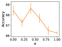
(a)

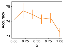
(b)

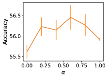
(c)

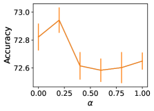
(d)

Figure 2: Balancing between BFS and DFS. $\alpha=0$ means just DFS while $\alpha=1$ means just BFS.

4.5 Ablation Study

We next report in Table 2 the results of our model’s ablation study. To this end, we remove each time a single component from the tBDFS model and measure its impact on performance. We explore a diverse set of ablations, as follows:

-DFS (-BFS): We remove the DFS (BFS) representation from the final node representation, ending up with merely a BFS (DFS) representation; setting $\alpha=1$ ($\alpha=0$). As can be noticed, removing the BFS representation or the DFS representation, considerably degrades the performance. This demonstrates that, there is no “correct” way to observe a graph, but rather by the combination of the two representations. This result was observed in many tasks on graphs. Most relevant to our work, it was observed in graph representation learning, e.g,  (Grover and Leskovec 2016) combined BFS and DFS walks during the random walks.

path-avg: We switch the attention aggregation of the path, as presented in Eq. 6, to an average aggregation instead. As we can observe, the performance degrades over all datasets and metrics. This demonstrates the importance of a smart aggregation layer over nodes in a given path.

paths-avg: We switch the paths attention aggregation, as presented in Eq. 7, to an average aggregation instead. We observe that the performance degrades in 7 out of the 10 metrics, while additional 2 remain with similar performance. We note that during the previous step (see Eq. 6), we could potentially learn that a given path is uninformative for the target node. This implies that the second step only fine-tunes the path representations from the previous step; explaining why this ablation is less effective than the “path-avg” ablation.

-time: We remove the time information in two manners: (1) In the time encoder, for any given $\Delta t$, we set $\Phi(\Delta t)=\bar{0}$; (2) The future neighbors are not masked as explained in Eq. 2. As we can see, removing the time information greatly degrades the performance also compared to the other temporal baselines. This reinforces the importance of dedicated temporal GNN architectures that leverage the temporal data.

5 Conclusions

We have explored a novel approach to observe temporal graphs. Most prior GNN works have proposed a layer that learns a node representation by aggregating information from its historical neighbors. Unlike prior GNN works, which have applied learning using a Breath-First Search (BFS) traversal over historical neighbors, we tackled the learning task from a different perspective and proposed a layer that aggregates over temporal paths ending at a given target node. The core idea of our approach lies in learning patterns using a Depth-First Search (DFS) traversal. Such a traversal has a better potential of explaining how messages have “travelled” in the graph until they have reached a desired target. The DFS representation was produced by first learning a representation for each temporal path ending in a given target node, and then aggregating all path representations into a final node representation. We empirically showed that tBDFS method outperforms state-of-the-art baselines on the temporal link prediction task, over a variety of different temporal graph datasets. To the best of our knowledge, we are the first to apply a temporal-DFS neural-network. We do not add new information to a node, but rather observe the same information by a new perspective. As future work, we wish to explore the effect of longer temporal paths and additional perspectives aside from BFS and DFS.

References

- Belkin and Niyogi (2001) Belkin, M.; and Niyogi, P. 2001. Laplacian eigenmaps and spectral techniques for embedding and clustering. In Advances in Neural Information Processing Systems, volume 14, 585–591.
- Cai, Zheng, and Chang (2018) Cai, H.; Zheng, V. W.; and Chang, K. C.-C. 2018. A comprehensive survey of graph embedding: Problems, techniques, and applications. IEEE Transactions on Knowledge and Data Engineering, 30(9): 1616–1637.
- Cao, Lu, and Xu (2015) Cao, S.; Lu, W.; and Xu, Q. 2015. Grarep: Learning graph representations with global structural information. In Proceedings of the 24th ACM international on conference on information and knowledge management, 891–900.
- Chen et al. (2021) Chen, J.; Wang, Y.; Zeng, M.; Xiang, Z.; and Ren, Y. 2021. Graph Attention Networks with LSTM-based Path Reweighting. arXiv:2106.10866.
- Cui et al. (2018) Cui, Z.; Henrickson, K.; Ke, R.; and Wang, Y. 2018. High-Order Graph Convolutional Recurrent Neural Network. arXiv preprint.
- da Xu et al. (2020) da Xu; chuanwei ruan; evren korpeoglu; sushant kumar; and kannan achan. 2020. Inductive representation learning on temporal graphs. In International Conference on Learning Representations (ICLR).
- Dunlavy, Kolda, and Acar (2011) Dunlavy, D. M.; Kolda, T. G.; and Acar, E. 2011. Temporal link prediction using matrix and tensor factorizations. TKDD, 5(2): 10.
- Feng et al. (2018) Feng, J.; Li, Y.; Zhang, C.; Sun, F.; Meng, F.; Guo, A.; and Jin, D. 2018. Deepmove: Predicting human mobility with attentional recurrent networks. In Proceedings of the 2018 world wide web conference, 1459–1468.
- Gilmer et al. (2017) Gilmer, J.; Schoenholz, S. S.; Riley, P. F.; Vinyals, O.; and Dahl, G. E. 2017. Neural message passing for quantum chemistry. In International conference on machine learning, 1263–1272. PMLR.
- Goldenberg et al. (2021) Goldenberg, D.; Kofman, K.; Levin, P.; Mizrachi, S.; Kafry, M.; and Nadav, G. 2021. Booking. com WSDM WebTour 2021 Challenge. In ACM WSDM Workshop on Web Tourism (WSDM WebTour’21).
- Grover and Leskovec (2016) Grover, A.; and Leskovec, J. 2016. node2vec: Scalable feature learning for networks. In Proceedings of the 22nd ACM SIGKDD international conference on Knowledge discovery and data mining, 855–864.
- Hamilton, Ying, and Leskovec (2017) Hamilton, W. L.; Ying, R.; and Leskovec, J. 2017. Inductive representation learning on large graphs. In Proceedings of the 31st International Conference on Neural Information Processing Systems, 1025–1035.
- Harper and Konstan (2015) Harper, F. M.; and Konstan, J. A. 2015. The movielens datasets: History and context. Acm transactions on interactive intelligent systems (tiis), 5(4): 1–19.
- Jain et al. (2016) Jain, A.; Zamir, A. R.; Savarese, S.; and Saxena, A. 2016. Structural-rnn: Deep learning on spatio-temporal graphs. In Proceedings of the ieee conference on computer vision and pattern recognition, 5308–5317.
- Kenton and Toutanova (2019) Kenton, J. D. M.-W. C.; and Toutanova, L. K. 2019. BERT: Pre-training of Deep Bidirectional Transformers for Language Understanding. In Proceedings of NAACL-HLT, 4171–4186.
- Kingma and Ba (2015) Kingma, D. P.; and Ba, J. 2015. Adam: A Method for Stochastic Optimization. In ICLR (Poster).
- Kipf and Welling (2016) Kipf, T. N.; and Welling, M. 2016. Variational Graph Auto-Encoders. NIPS Workshop on Bayesian Deep Learning.
- Kipf and Welling (2017) Kipf, T. N.; and Welling, M. 2017. Semi-supervised classification with graph convolutional networks. ICLR.
- Kumar et al. (2018) Kumar, S.; Hamilton, W. L.; Leskovec, J.; and Jurafsky, D. 2018. Community interaction and conflict on the web. In Proceedings of the 2018 World Wide Web Conference on World Wide Web, 933–943. International World Wide Web Conferences Steering Committee.
- Kumar, Zhang, and Leskovec (2019) Kumar, S.; Zhang, X.; and Leskovec, J. 2019. Predicting Dynamic Embedding Trajectory in Temporal Interaction Networks. In Proceedings of the 25th ACM SIGKDD international conference on Knowledge discovery and data mining. ACM.
- Lin et al. (2021) Lin, B.; Wang, X.; Dong, Y.; Huo, C.; Ren, W.; and Xu, C. 2021. Metapaths guided Neighbors aggregated Network for? Heterogeneous Graph Reasoning. arXiv preprint arXiv:2103.06474.
- Liu et al. (2019) Liu, Z.; Chen, C.; Li, L.; Zhou, J.; Li, X.; Song, L.; and Qi, Y. 2019. Geniepath: Graph neural networks with adaptive receptive paths. In Proceedings of the AAAI Conference on Artificial Intelligence, 4424–4431.
- Loomis (2013) Loomis, L. H. 2013. Introduction to abstract harmonic analysis. Courier Corporation.
- Mikolov et al. (2013) Mikolov, T.; Chen, K.; Corrado, G.; and Dean, J. 2013. Efficient Estimation of Word Representations in Vector Space. ICLR, abs/1301.3781.
- Nguyen et al. (2018) Nguyen, G. H.; Lee, J. B.; Rossi, R. A.; Ahmed, N. K.; Koh, E.; and Kim, S. 2018. Continuous-time dynamic network embeddings. In Proc. of WWW Companion, 969–976.
- Paszke et al. (2017) Paszke, A.; Gross, S.; Chintala, S.; Chanan, G.; Yang, E.; DeVito, Z.; Lin, Z.; Desmaison, A.; Antiga, L.; and Lerer, A. 2017. Automatic Differentiation in PyTorch. In NIPS 2017 Workshop on Autodiff.
- Perozzi, Al-Rfou, and Skiena (2014) Perozzi, B.; Al-Rfou, R.; and Skiena, S. 2014. Deepwalk: Online learning of social representations. In Proceedings of the 20th ACM SIGKDD international conference on Knowledge discovery and data mining, 701–710.
- Roweis and Saul (2000) Roweis, S. T.; and Saul, L. K. 2000. Nonlinear dimensionality reduction by locally linear embedding. SCIENCE, 290: 2323–2326.
- Schlichtkrull et al. (2018) Schlichtkrull, M.; Kipf, T. N.; Bloem, P.; Van Den Berg, R.; Titov, I.; and Welling, M. 2018. Modeling relational data with graph convolutional networks. In European semantic web conference, 593–607. Springer.
- Singer, Guy, and Radinsky (2019) Singer, U.; Guy, I.; and Radinsky, K. 2019. Node Embedding over Temporal Graphs. In Proceedings of IJCAI-19, 4605–4612. AAAI Press.
- Singer and Kira (2022) Singer, U.; and Kira, R. 2022. EqGNN: Equalized Node Opportunity in Graphs. In Proceedings of the AAAI conference on artificial intelligence.
- Singer, Radinsky, and Horvitz (2020) Singer, U.; Radinsky, K.; and Horvitz, E. 2020. On biases of attention in scientific discovery. Bioinformatics. Btaa1036.
- Skardinga, Gabrys, and Musial (2021) Skardinga, J.; Gabrys, B.; and Musial, K. 2021. Foundations and modelling of dynamic networks using dynamic graph neural networks: A survey. IEEE Access.
- Tenenbaum, De Silva, and Langford (2000) Tenenbaum, J. B.; De Silva, V.; and Langford, J. C. 2000. A global geometric framework for nonlinear dimensionality reduction. science, 290(5500): 2319–2323.
- Vaswani et al. (2017) Vaswani, A.; Shazeer, N.; Parmar, N.; Uszkoreit, J.; Jones, L.; Gomez, A. N.; Kaiser, Ł.; and Polosukhin, I. 2017. Attention is all you need. In Advances in neural information processing systems, 5998–6008.
- Veličković et al. (2017) Veličković, P.; Cucurull, G.; Casanova, A.; Romero, A.; Lio, P.; and Bengio, Y. 2017. Graph attention networks. International Conference on Learning Representations.
- Wang and Li (2017) Wang, H.; and Li, Z. 2017. Region Representation Learning via Mobility Flow. In Proceedings of the 2017 ACM on Conference on Information and Knowledge Management, 237–246.
- Wu et al. (2020) Wu, Z.; Pan, S.; Chen, F.; Long, G.; Zhang, C.; and Philip, S. Y. 2020. A comprehensive survey on graph neural networks. IEEE Transactions on Neural Networks and Learning Systems.
- Yan, Xiong, and Lin (2018) Yan, S.; Xiong, Y.; and Lin, D. 2018. Spatial Temporal Graph Convolutional Networks for Skeleton-Based Action Recognition. In Proceedings of the AAAI conference on artificial intelligence, volume 32.
- Yan et al. (2006) Yan, S.; Xu, D.; Zhang, B.; Zhang, H.-J.; Yang, Q.; and Lin, S. 2006. Graph embedding and extensions: A general framework for dimensionality reduction. IEEE transactions on pattern analysis and machine intelligence, 29(1): 40–51.
- Yang et al. (2019) Yang, Y.; Wang, X.; Song, M.; Yuan, J.; and Tao, D. 2019. SPAGAN: Shortest Path Graph Attention Network. In Proceedings of IJCAI-19, IJCAI’19, 4099–4105. AAAI Press. ISBN 9780999241141.
- Ying et al. (2021) Ying, C.; Cai, T.; Luo, S.; Zheng, S.; Ke, G.; He, D.; Shen, Y.; and Liu, T.-Y. 2021. Do Transformers Really Perform Badly for Graph Representation? In Thirty-Fifth Conference on Neural Information Processing Systems.
- Ying et al. (2018) Ying, R.; You, J.; Morris, C.; Ren, X.; Hamilton, W. L.; and Leskovec, J. 2018. Hierarchical graph representation learning with differentiable pooling. arXiv preprint arXiv:1806.08804.
- Yu, Yin, and Zhu (2018) Yu, B.; Yin, H.; and Zhu, Z. 2018. Spatio-temporal Graph Convolutional Neural Network. IJCAI.
- Yu, Aggarwal, and Wang (2017) Yu, W.; Aggarwal, C. C.; and Wang, W. 2017. Temporally factorized network modeling for evolutionary network analysis. In Proceedings of the Tenth ACM International Conference on Web Search and Data Mining, 455–464.