Solving the Poisson equation using coupled Markov chains

Abstract

This article shows how coupled Markov chains that meet exactly after a random number of iterations can be used to generate unbiased estimators of the solutions of the Poisson equation. We establish connections to recently-proposed unbiased estimators of Markov chain equilibrium expectations. We further employ the proposed estimators of solutions of the Poisson equation to construct unbiased estimators of the asymptotic variance of Markov chain ergodic averages, involving a random but finite computing time. We formally study the proposed methods under realistic assumptions on the meeting times of the coupled chains and on the existence of moments of test functions under the target distribution. We describe experiments in toy examples such as the autoregressive model, and in more challenging settings.

1 Introduction

1.1 Central Limit Theorem and the Poisson equation

Markov chain Monte Carlo (MCMC) methods form a convenient family of simulation techniques with many applications in statistics. With $(\mathbb{X},\mathcal{X})$ a measurable space and $\pi$ a probability measure of statistical interest, MCMC involves simulation of a discrete-time, time-homogeneous Markov chain $X=(X_{t})_{t\geq 0}$, with a $\pi$-invariant Markov transition kernel $P$ and some initial distribution $\pi_{0}$. Letting $L^{p}(\pi)=\{f:\pi(\left|f\right|^{p})<\infty\}$, where $\pi(f)=\int f(x)\pi({\rm d}x)$, the interest is to approximate $\pi(h)$ for some function $h\in L^{1}(\pi)$.

In particular, after simulating the chain until time $t$, one may approximate an integral of interest $\pi(h)$ via the average $t^{-1}\sum_{s=0}^{t-1}h(X_{s})$. Under weak assumptions, such averages converge almost surely to $\pi(h)$ as $t\to\infty$, and under stronger but still realistic assumptions on $\pi_{0}$, $P$ and $h$ that hold in many applications, they satisfy central limit theorems (CLTs),

$$\sqrt{t}\left(\frac{1}{t}\sum_{s=0}^{t-1}h(X_{s})-\pi(h)\right)\overset{d}{\to}N(0,v(P,h)),\qquad\text{as }t\to\infty,$$ (1.1)

where $v(P,h)$ is the asymptotic variance associated with the Markov kernel $P$ and the function $h$ (see, e.g., Jones, 2004). One standard route to proving a CLT is via a solution of the Poisson equation for $h$ associated with $P$, i.e. any function $g$ such that

$$(I-P)g=h-\pi(h)=:h_{0},$$ (1.2)

where $P$ is viewed as a Markov operator and $I$ is the identity. In particular, if $h,g\in L^{2}(\pi)$ then (1.1) holds with initial distribution $\pi$ by Douc et al. (2018, Theorem 21.2.5), and

$$v(P,h)=\mathbb{E}_{\pi}\left[\left\{g(X_{1})-Pg(X_{0})\right\}^{2}\right]=2\pi(h_{0}\cdot g)-\pi(h_{0}^{2}),$$ (1.3)

where $\mathbb{E}_{\pi}$ indicates that $X_{0}\sim\pi$. We focus on solutions $g=g_{\star}+c$ with $g_{\star}$ defined as follows.

Definition 1.

Let $h\in L^{1}(\pi)$, define $h_{0}=h-\pi(h)$ and the function

$$g_{\star}:=\sum_{t=0}^{\infty}P^{t}h_{0}.$$ (1.4)

If $g_{\star}$ is well-defined, then it is straightforward to deduce that $(I-P)g_{\star}=h_{0},$ so that $g_{\star}$ is indeed fishy. In addition, $g_{\star}+c$ is fishy for any constant $c\in\mathbb{R}$. Moreover, if $g_{\star}\in L^{1}(\pi)$ then $\pi(g_{\star})=0$, and by Douc et al. (Lemma 21.2.2, 2018) any other fishy function $g$ is equal to $g_{\star}$ up to an additive constant. Inserting the function $g_{\star}$ in place of $g$ in (1.3) leads to the expression

$$v(P,h)={\rm var}_{\pi}(h(X_{0}))+2\sum_{t=1}^{\infty}{\rm cov}_{\pi}(h(X_{0}),h(X_{t})),$$ (1.5)

where the subscript $\pi$ indicates that $X_{0}\sim\pi$. That familiar expression can be obtained with simple calculations from $\lim_{t\to\infty}{\rm var}_{\pi}(t^{-1/2}\sum_{s=0}^{t-1}h(X_{s}))$.

1.2 Monte Carlo methods using the Poisson equation

Despite its convenience for theoretical analysis, the Poisson equation is not analytically solvable for most Markov chains and functions of interest, and consistent approximations have been lacking. As a result, the asymptotic variance $v(P,h)$ is commonly estimated using batch-means, spectral variance (see, e.g., Flegal & Jones, 2010; Vats et al., 2018, 2019; Chakraborty et al., 2022), or initial sequence estimators (Geyer, 1992; Berg & Song, 2022). On the other hand, inconsistent approximations of the solution of the Poisson equation have been proposed for the purpose of variance reduction via control variates. This involves replacing $h$ by $h-\phi$ in an ergodic average, where $\phi\in L_{0}^{1}(\pi)=\{f\in L^{1}(\pi):\pi(f)=0\}$, so that $\pi(h-\phi)=\pi(h)$ and the limit of the MCMC estimator is unchanged, but the variance may be smaller with a judicious choice of $\phi$. A convenient family of $\phi$ is $\{(I-P)f:f\in L^{1}(\pi)\}$ since $\phi\in L_{0}^{1}(\pi)$ by construction and indeed an optimal choice of $f$ is $g$. Approximations of $g$ have been considered for this purpose in, e.g., Andradóttir et al. (1993); Henderson (1997); Dellaportas & Kontoyiannis (2012); Mijatović & Vogrinc (2018); Alexopoulos et al. (2023).

We aim to contribute to methodological aspects of the Poisson equation, with a focus on asymptotic variance estimation via (1.3). We develop novel approximations of the solution $g$, which are unbiased under fairly weak conditions, using coupled Markov chains. Couplings have often been used as formal techniques to analyze the marginal convergence of Markov chains (e.g. Jerrum, 1998), but many couplings are also implementable, with applications to exact sampling (Propp & Wilson, 1996), unbiased estimation (Glynn & Rhee, 2014), convergence diagnostics (Johnson, 1996), or variance reduction (Neal & Pinto, 2001). Here we find new uses for couplings of MCMC algorithms: in Section 2 we propose unbiased estimators of evaluations of the solution $g$. Then we find strong connections between these estimators and the family of unbiased estimators of $\pi(h)$ pioneered by Glynn & Rhee (2014), which we leverage to obtain new results on unbiased MCMC (Jacob et al., 2020). In Section 3 we use the proposed estimators of $g$ to approximate (1.3) in combination with unbiased MCMC, leading to novel estimators of $v(P,h)$ that are unbiased and with finite variance under fairly mild conditions. The proposed asymptotic variance estimators are studied numerically in Section 4.

2 Coupled chains and fishy functions

2.1 Coupled Markov chains

For a given $\pi$-invariant Markov kernel $P$, we consider the time-homogeneous, discrete-time Markov chain $(X,Y)=(X_{t},Y_{t})_{t\geq 0}$ with Markov kernel $\bar{P}$, which is a “faithful” coupling of $P$ with itself (Rosenthal, 1997), i.e. it satisfies

$$\bar{P}(x,y;A\times\mathbb{X})=P(x,A),\quad\bar{P}(x,y;\mathbb{X}\times A)=P(y,A),\qquad A\in\mathcal{X},$$ (2.1)

and $\bar{P}(x,x;\{(x^{\prime},y^{\prime}):x^{\prime}=y^{\prime}\})=1$ for all $x\in\mathbb{X}$. We observe that $X=(X_{t})_{t\geq 0}$ and $Y=(Y_{t})_{t\geq 0}$ are both time-homogeneous, discrete-time Markov chains with kernel $P$. We use subscripts to denote the distribution of $(X_{0},Y_{0})$. For example $\mathbb{P}_{x,y}$ is the law of $(X,Y)$ when $(X_{0},Y_{0})=(x,y)$, and $\mathbb{P}_{\nu}$ indicates $(X_{0},Y_{0})\sim\nu$. When only one chain is referenced, e.g. $X$, we may similarly write $\mathbb{P}_{x}$ and $\mathbb{P}_{\mu}$ to indicate $X_{0}=x$ and $X_{0}\sim\mu$, respectively. An important random variable when using coupled Markov chains is the meeting time,

$$\tau:=\inf\{t\geq 0:X_{t}=Y_{t}\},$$ (2.2)

which is the first time at which $X$ and $Y$ take the same value. Since $\bar{P}$ is faithful, $X_{t}=Y_{t}$ with probability $1$ for all times $t\geq\tau$. Johnson (1998); Jacob et al. (2020) and others have shown how to construct the coupled kernel $\bar{P}$ for various MCMC algorithms, such that $\tau$ has finite expectation; see Appendix A for pointers.

The main assumption throughout this paper is that $\tau$ has a finite $\kappa$th moment, $\kappa>1$, when $(X_{0},Y_{0})\sim\pi\otimes\pi$, the product measure of $\pi$ and itself.

Assumption 2.

The Markov kernel $P$ is $\pi$-irreducible and for some $\kappa>1$, $\mathbb{E}_{\pi\otimes\pi}[\tau^{\kappa}]<\infty.$

The assumption implies a polynomially decaying survival function $\mathbb{P}_{x,y}(\tau>t)$ of order $\kappa$ and, conversely, one may verify the assumption by showing that $\mathbb{P}_{x,y}(\tau>t)$ decays polynomially with order $s>\kappa$ with a dependence on $(x,y)$ that is not too strong. The proof of the next result is in Appendix D.1.

Proposition 3.

If Assumption 2 holds then for all $t\geq 0$,

$$\mathbb{P}_{x,y}(\tau>t)\leq\mathbb{E}_{x,y}[\tau^{\kappa}](t+1)^{-\kappa},$$

and $\mathbb{E}_{x,y}[\tau^{\kappa}]<\infty$ for $\pi\otimes\pi$-almost all $(x,y)$. Conversely, if for some $s>\kappa$, there exists $\tilde{C}:\mathbb{X}\times\mathbb{X}\to\mathbb{R}$ with $\pi\otimes\pi(\tilde{C})<\infty$ such that for $\pi\otimes\pi$-almost all $(x,y)$, we have for all $t\geq 0$,

$$\mathbb{P}_{x,y}(\tau>t)\leq\tilde{C}(x,y)(t+1)^{-s},$$

then $\mathbb{E}_{\pi\otimes\pi}\left[\tau^{\kappa}\right]<\infty$.

Our assumption on the moments of the meeting time allows us to employ the CLT of Theorem 4, that provides that the expression of $v(P,h)$ at the basis of our proposed estimators in Section 3. The proof in Appendix D.2 relies heavily on the strategy of Douc et al. (2018, Section 21.4.1) but features $g_{\star}$ from Definition 1 more prominently, and uses the CLT condition from Maxwell & Woodroofe (2000) rather than Douc et al. (2018, Theorem 21.4.1). Note that the CLT does not require $g_{\star}\in L_{0}^{2}(\pi)$.

Theorem 4.

Under Assumption 2, let $h\in L^{m}(\pi)$ for some $m>2\kappa/(\kappa-1)$. Then $g_{\star}\in L_{0}^{1}(\pi)$, $h_{0}\cdot g_{\star}\in L^{1}(\pi)$ and the CLT (1.1) holds for $\pi$-almost all $X_{0}$ with $v(P,h)=2\pi(h_{0}\cdot g_{\star})-\pi(h_{0}^{2})<\infty$.

2.2 Unbiased approximation of fishy functions

In the Markov chain setting, solutions of the Poisson equation for $h$, or fishy functions for brevity, have been studied extensively (see, e.g., Duflo, 1970; Glynn & Meyn, 1996; Glynn & Infanger, 2022). It is known, for example, that fishy functions exist under fairly weak conditions. We focus on the particular, and more restrictive, core expression of $g_{\star}$ from Definition 1.

Although $g_{\star}$ is not necessarily well-defined $\pi$-almost everywhere in general, Assumption 2 implies that for $p\geq 1$, $g_{\star}\in L^{p}(\pi)$ for $h\in L^{m}(\pi)$ when $\kappa$ and $m$ are sufficiently large in relation to $p$; see Theorem 24. We now define a family of fishy functions that will play a central role in what follows.

Definition 5.

For $y\in\mathbb{X}$, the function

$$g_{y}:x\mapsto g_{\star}(x)-g_{\star}(y),$$ (2.3)

is fishy if $g_{\star}$ is well-defined, since $g_{\star}(y)$ is a constant. When $y$ is fixed, in the sequel we may write $g$ instead of $g_{y}$.

A priori, links between couplings of Markov chains and fishy functions may not appear as obvious. However, the definition of $g_{y}$ lends itself naturally to unbiased approximation via coupled Markov chains.

Definition 6.

For $x\in\mathbb{X}$, the proposed estimator of $g_{y}(x)$ is, with $(X_{0},Y_{0})=(x,y)$,

$$G_{y}(x):=\sum_{t=0}^{\tau-1}h(X_{t})-h(Y_{t}),$$ (2.4)

where $(X,Y)$ and $\tau$ are defined in Section 2.1. In particular, the dependence of $G_{y}(x)$ on $x$ and $y$ is that the law of $(X,Y)$ is $\mathbb{P}_{x,y}$ in (2.4), and so we may omit the subscript $(x,y)$ when there is no ambiguity. We will also denote $G_{y}$ by $G$ below, in places where the explicit mention of $y$ is unnecessary.

The simple intuition behind Definition 6 is that we can equivalently write

$$G_{y}(x)=\sum_{t=0}^{\infty}h(X_{t})-h(Y_{t})=\sum_{t=0}^{\infty}h_{0}(X_{t})-h_{0}(Y_{t}),$$

and upon justifying the interchange of expectation and infinite sum as we do in Appendix D.3,

$$\mathbb{E}\left[G_{y}(x)\right]=\sum_{t=0}^{\infty}P^{t}h_{0}(x)-\sum_{t=0}^{\infty}P^{t}h_{0}(y)=g_{\star}(x)-g_{\star}(y).$$

We have the following, which is established in Appendix D.3 as a special case of Theorem 34.

Theorem 7.

Under Assumption 2, let $h\in L^{m}(\pi)$ for some $m>\kappa/(\kappa-1)$. For $\pi\otimes\pi$-almost all $(x,y)$, $\mathbb{E}\left[G_{y}(x)\right]=g_{\star}(x)-g_{\star}(y)$ and for $p\geq 1$ such that $\frac{1}{p}>\frac{1}{m}+\frac{1}{\kappa}$, $\mathbb{E}\left[\left|G_{y}(x)\right|^{p}\right]<\infty$.

Theorem 34 in Appendix D.3, also provides bounds on moments of $\left|G_{y}(x)\right|$. For our subsequent analysis of asymptotic variance estimators, it is important that this is a pointwise result. The random variable $G_{y}(x)$ may be simulated using Algorithm 2.1 with $L=0$. The cost of sampling $G_{y}(x)$ is the cost of running a pair of chains until they meet, which is typically comparable to twice the cost of running one chain for the same number of steps, i.e. $2\mathbb{E}_{x,y}[\tau]$ on average.

As a generalization of Definition 6 we might sample $Y_{0}\sim\nu$, for an arbitrary distribution $\nu$, and then generate $G_{Y_{0}}(x)$ given $Y_{0}$, which, under adequate assumptions, would be unbiased for the fishy function

$$g_{\nu}:x\mapsto g_{\star}(x)-\nu(g_{\star}).$$ (2.5)

Input: initial states $x$, $y$, Markov kernel $P$, coupled kernel $\bar{P}$, lag $L\geq 0$.

1. Set $X_{0}=x$, $Y_{0}=y$.

2. If $L\geq 1$, for $t=1,\ldots,L$, sample $X_{t}$ from $P(X_{t-1},\cdot)$.

3. For $t\geq L$, sample $(X_{t+1},Y_{t-L+1})$ from $\bar{P}((X_{t},Y_{t-L}),\cdot)$ until $X_{t+1}=Y_{t-L+1}$.

Output: coupled chains and the meeting time defined as the smallest $t$ at which $X_{t}=Y_{t-L}$.

Algorithm 2.1 Simulation of coupled lagged chains.

Remark 8.

The above reasoning demonstrates how one can approximate the difference between two fishy function evaluations. In contrast, to unbiasedly approximate $g_{\star}(x)$ we would need to estimate $g_{\nu}(x)$ and $\pi(g_{\nu})$ in an unbiased manner, for an arbitrary distribution $\nu$, and take their difference.

An alternative estimator to Definition 6 could employ a random “truncation” variable as in Glynn & Rhee (2014) or Agapiou et al. (2018). This would allow the use of coupled chains that do not exactly meet, as long as the distance between them goes to zero fast enough. We do not pursue this generalization here, as exact meetings can be obtained in a variety of MCMC settings (Jacob et al., 2020).

2.3 Recovering Glynn–Rhee estimators

Through the Poisson equation we can recover the unbiased estimation techniques of Glynn & Rhee (2014) and Jacob et al. (2020). First observe that we may rearrange (1.2) as

$$\pi(h)=h(x)+Pg(x)-g(x),\qquad x\in\mathbb{X},$$ (2.6)

where the left-hand side does not depend on $x$ and $g$ is any fishy function for $h$. It then seems natural to estimate $\pi(h)$ by estimating the terms on the right-hand side, for any $x$. With $g=g_{\star}$ we may write

$$\pi(h)=h(x)+\sum_{t=0}^{\infty}P^{t+1}h(x)-P^{t}h(x),$$ (2.7)

where the right-hand side is a familiar quantity in the light of Glynn & Rhee (2014). In particular, one may run Algorithm 2.1 with $L=1$: starting from $X_{0}=Y_{0}=x$, sample $X_{1}\sim P(X_{0},\cdot)$, and iteratively sample $(X_{t+1},Y_{t})\sim\bar{P}((X_{t},Y_{t-1}),\cdot)$ for $t\geq 1$, where $\bar{P}$ is as defined in Section 2.1. The generated $(X,Y)$ process is such that $(X_{t+L},Y_{t})_{t\geq 0}$ is Markov and $X_{t+L}=Y_{t}$ almost surely for all $t$ large enough. Since $P^{t}h(x)$ is the expectation of both $h(X_{t})$ and $h(Y_{t})$, the estimator $X_{0}+\sum_{t=0}^{\infty}\{h(X_{t+1})-h(Y_{t})\}$ is unbiased for $\pi(h)$ under suitable assumptions.

This same perspective on (2.6) suggests that for any $x\in\mathbb{X}$ we may define the equivalent and notationally convenient approximation $h(x)+G_{x}(X_{1})$, where $X_{1}\sim P(x,\cdot)$, and it is clear that if $\mathbb{E}[G_{y^{\prime}}(x^{\prime})]=g_{y^{\prime}}(x^{\prime})$ for $\pi$-almost all $x^{\prime}$ and $y^{\prime}=x$, then

$$\mathbb{E}_{x}\left[h(x)+G_{x}(X_{1})\right] =h(x)+\mathbb{E}_{x}\left[g_{x}(X_{1})\right]$$

$$=h(x)+\mathbb{E}_{x}\left[g_{\star}(X_{1})\right]-g_{\star}(x)$$

$$=h(x)+Pg_{\star}(x)-g_{\star}(x)$$

$$=\pi(h).$$

The initialization of the chains can be generalized from a point mass at $x\in\mathbb{X}$ to any probability distribution $\pi_{0}$. Indeed, a re-arranged and integrated Poisson equation is

$$\pi(h)=\pi_{0}(h)+\pi_{0}P(g)-\pi_{0}(g),$$ (2.8)

and this suggests the following estimator of $\pi(h)$, with essentially the same justification as above.

Definition 9.

For $h\in L^{1}(\pi)$, denote the approximation of $\pi(h)$ by

$$H=h(X_{0}^{\prime})+G_{Y_{0}^{\prime}}(X_{1}^{\prime}),$$ (2.9)

where marginally $X_{0}^{\prime}\sim\mu$, $Y_{0}^{\prime}\sim\mu$ and $X_{1}^{\prime}\sim\mu P$ for some probability measure $\mu$. We denote by $\gamma$ the joint probability measure for $(X_{1}^{\prime},Y_{0}^{\prime})$, since this features in our analysis, noting that this is a coupling of $\mu P$ and $\mu$.

The estimator in Definition 9 is identical to the estimator denoted by $H_{0}(X,Y)$ in Jacob et al. (2020) if one chooses $X_{1}^{\prime}\sim P(X_{0}^{\prime},\cdot)$ and $(X_{0}^{\prime},Y_{0}^{\prime})$ is drawn from some coupling of $\mu=\pi_{0}$ with itself. We can also retrieve the more efficient variants proposed in Jacob et al. (2020). By changing the initial distribution $\gamma$, Definition 9 also admits the estimators denoted by $H_{k}(X,Y)$ for some $k\in\mathbb{N}$ in Jacob et al. (2020), and the estimators denoted by $H_{k:m}(X,Y)$ are obtained as averages of $H_{k}(X,Y)$ over a range of values of $k$. Unbiased estimators based on chains coupled with a lag $L>1$ (Vanetti & Doucet, 2020) can be retrieved as well by considering the Poisson equation associated with the iterated Markov kernel $P^{L}$. To make this precise, we make the following definition.

Definition 10.

The $L$-lagged and $k$-offset approximation of $\pi(h)$ is

$$H_{k}^{(L)}:=h(X_{k}^{\prime})+\sum_{j=1}^{\infty}h(X_{k+jL}^{\prime})-h(Y_{k+(j-1)L}^{\prime}),$$

where $k\in\mathbb{N}$, $L\in\mathbb{N}$, $(X_{t+L}^{\prime},Y_{t}^{\prime})_{t\geq 0}$ is a time-homogeneous Markov chain with Markov kernel $\bar{P}$ , and $(X_{t}^{\prime})_{t=0}^{L}$ is a Markov chain with transition kernel $P$ and initial distribution $\pi_{0}$ and $Y^{\prime}_{0}\sim\pi_{0}$ independent of $(X^{\prime}_{0:L})$. In particular, $(X_{L}^{\prime},Y^{\prime}_{0})\sim\gamma^{(L)}=\pi_{0}P^{L}\otimes\pi_{0}$. We also define for any $k,\ell\in\mathbb{N}$ with $k\leq\ell$, the average of such estimators as

$$H_{k:\ell}^{(L)}:=\frac{1}{\ell-k+1}\sum_{t=k}^{\ell}H_{t}^{(L)}.$$

The following result is established in Appendix D.4, as a particular case of Proposition 40, where upper bounds are given for $\mathbb{E}[|H_{k:\ell}^{(L)}|^{p}]$. This result can be compared with Jacob et al. (Proposition 1, 2020) and Middleton et al. (Theorem 1, 2020), which provide only finite second moments. The latter obtains the same conditions on $\kappa$ and $m$ for $p=2$. The bounded ${\rm d}\pi_{0}/{\rm d}\pi$ assumption allows one to avoid the less explicit assumption that $\sup_{n\geq 0}\mu P^{n}(|h|^{2+\eta})<\infty$ and can often be verified in practice.

Theorem 11.

Under Assumption 2, let $h\in L^{m}(\pi)$ with $m>\kappa/(\kappa-1)$, and ${\rm d}\pi_{0}/{\rm d}\pi\leq M$ with $M<\infty$. Then for any $k,\ell\in\mathbb{N}$ with $k\leq\ell$, $\mathbb{E}[H_{k:\ell}^{(L)}]=\pi(h)$ and for $p\geq 1$ such that $\frac{1}{p}>\frac{1}{m}+\frac{1}{\kappa}$, $\mathbb{E}[|H_{k:\ell}^{(L)}|^{p}]<\infty$.

Remark 12.

By Theorem 11 it is sufficient that $\kappa>2$ and $m>2\kappa/(\kappa-2)$ for $H$ to have a finite variance. On the other hand, Theorem 4 implies that a CLT holds for $h$ if $\kappa>1$ and $m>2\kappa/(\kappa-1)$, which is weaker. The stronger condition in Theorem 11 is because finite second moment of the unbiased estimator is shown via finite second moment of the approximation of $g_{\star}$, and this requires $g_{\star}\in L_{0}^{2}(\pi)$.

Remark 13.

There are known links between bias of MCMC estimators and fishy functions. Kontoyiannis & Dellaportas (2009, Section 4) observe that the average $t^{-1}\sum_{s=0}^{t-1}h(X_{s})$ has expectation $t^{-1}\sum_{s=0}^{t-1}P^{s}h(x_{0})$ given $X_{0}=x$, thus $g_{\star}(x)$ represents the leading term in the asymptotic bias:

$$g_{\star}(x)=\lim_{t\to\infty}t\left\{\mathbb{E}_{x}\left[t^{-1}\sum_{s=0}^{t-1}h(X_{s})\right]-\pi(h)\right\}.$$ (2.10)

To numerically quantify that asymptotic bias, if $g_{\star}\in L_{0}^{1}(\pi)$ and an approximation of $g=g_{\star}+c$ is available, we may use the identity $g_{\star}=g-\pi(g)$ to approximate $g_{\star}$. On the other hand, even without accounting for $c$, the behaviour of $g$ may be informative about the asymptotic bias, e.g. how $g(x)$ changes as $|x|$ increases, as illustrated in Section 4.1.

2.4 Subsampled unbiased estimators

In practice, it can be convenient to view the estimator $H_{k:\ell}^{(L)}$ in Definition 10 as equivalent to the integral of $h$ with respect to an unbiased signed measure $\hat{\pi}$; details are presented in Appendix B. This perspective allow us to define a subsampled version of the estimator with lower computational cost, for example if evaluations of $h$ are expensive in comparison to the simulation of $\hat{\pi}$, and this is particularly beneficial for the asymptotic variance estimator proposed in the sequel. The computational benefits of subsampling in this context are related to the thinning ideas in Owen (2017).

The following result is established in Appendix D.4 as a simplification of Proposition 42. It demonstrates that the sufficient conditions for lack-of-bias and finite $p$th moments are identical for both $H_{k:\ell}^{(L)}$ and the subsampled estimator $S_{R}$ for any $R\geq 1$.

Theorem 14.

Under Assumption 2, let $h\in L^{m}(\pi)$ for some $m>\kappa/(\kappa-1)$, ${\rm d}\pi_{0}/{\rm d}\pi\leq M$, $k,\ell\in\mathbb{N}$ with $k\leq\ell$, and $\hat{\pi}=\sum_{i=1}^{N}\omega_{i}\delta_{Z_{i}}$ be the unbiased signed measure associated with $H_{k:\ell}^{(L)}$. Define for some $R\geq 1$,

$$S_{R}=\frac{1}{R}\sum_{i=1}^{R}N\omega_{I_{i}}h(Z_{I_{i}}),$$

where $I_{1},\ldots,I_{R}$ are conditionally independent ${\rm Categorial}\{\xi_{1},\ldots,\xi_{N}\}$ random variables with

$$\frac{a}{N}\leq\min_{i}\xi_{i}\leq\max_{i}\xi_{i}\leq\frac{b}{N},$$

for some constants $0<a\leq b<\infty$ independent of $N$. Then $\mathbb{E}[S_{R}]=\pi(h)$ and for $p\geq 1$ such that $\frac{1}{p}>\frac{1}{m}+\frac{1}{\kappa}$, $\mathbb{E}\left[\left|S_{R}\right|^{p}\right]<\infty$.

Remark 15.

The more detailed Proposition 42 in Appendix D.4 provides a bound on $\mathbb{E}\left[\left|S_{R}\right|^{p}\right]^{\frac{1}{p}}$ but this bound does not depend on the value of $R$. For $p=2$, we can see that increasing $R$ decreases the variance of $S_{R}$, through the law of total variance

$${\rm var}\left(S_{R}\right) =\mathbb{E}\left[{\rm var}(S_{R}\mid\hat{\pi})\right]+{\rm var}\left(\mathbb{E}\left[S_{R}\mid\hat{\pi}\right]\right)$$

$$=\frac{1}{R}\mathbb{E}\left[{\rm var}(S_{1}\mid\hat{\pi})\right]+{\rm var}(\hat{\pi}(h)).$$

Hence, there is a tradeoff between computational cost and variance, with increasing $R$ potentially improving efficiency up to point where the variance is dominated by ${\rm var}(\hat{\pi}(h))$.

3 Asymptotic variance estimation

3.1 Ergodic Poisson asymptotic variance estimator

We consider the task of estimating the asymptotic variance in the CLT, $v(P,h)$ in (1.3). Various techniques have been proposed to estimate $v(P,h)$ from one or multiple MCMC runs (see the references provided in Section 1.2), and these estimators are consistent when the length of each chain goes to infinity. Here we employ coupled Markov chains, as generated by Algorithm 2.1, to define new estimators of $v(P,h)$: we start with a consistent estimator before introducing unbiased estimators in the next section. We first re-express (1.3) as

$$v(P,h) =-v(\pi,h)+2\pi((h-\pi(h))\cdot g),$$ (3.1)

where $v(\pi,h)$ is the variance of $h(X)$ under $X\sim\pi$. Expectations with respect to $\pi$ can be consistently estimated from long MCMC runs. Using $t$ steps after burn-in we define the empirical measure $\pi^{\text{MC}}=t^{-1}\sum_{s=0}^{t-1}\delta_{X_{s}}$. We can thus approximate $\pi(h)$ and $v(\pi,h)$ using the empirical mean and variance, denoted by $\pi^{\text{MC}}(h)$ and $v^{\text{MC}}(h)$, and these are typically consistent as $t\to\infty$.

The difficulty is in the term $\pi((h-\pi(h))\cdot g)$ in (3.1), since $g$ cannot be evaluated exactly. We employ unbiased estimators $G(x)$ in Definition 6 in place of evaluations $g(x)$. This leads to the following estimator of $v(P,h)$, which we call the ergodic Poisson asymptotic variance estimator (EPAVE),

$$\hat{v}(P,h)=-v^{\text{MC}}(h)+\frac{2}{t}\sum_{s=0}^{t-1}(h(X_{s})-\pi^{\text{MC}}(h))\cdot G(X_{s}),$$ (3.2)

where each $G(X_{s})$ is conditionally independent of all others given $(X_{0},\ldots,X_{t-1})$. The proposed EPAVE might be practically relevant, but in this paper we view it as an intermediate step toward the estimators of Section 3.2, which have the advantage of being unbiased.

Remark 16.

We can compute (3.2) online by keeping track of the sums

$$\sum_{s}h(X_{s}),\sum_{s}h(X_{s})^{2},\sum_{s}G(X_{s}),\sum_{s}h(X_{s})G(X_{s}).$$

We can also modulate the relative cost of estimating the fishy function evaluations in (3.2) by generating $G(X_{s})$ only for some of the times, e.g. when $s\mod D=0$ for some $D\in\mathbb{N}$, which amounts to a thinning strategy.

In Appendix D.7, we show that this estimator is strongly consistent and satisfies a $\sqrt{t}$-CLT under Assumption 2 and moment assumptions on $h$. The following summarizes Proposition 52 and Theorem 53. An expression for the asymptotic variance can be extracted from the proof, which depends implicitly on the coupling used to define $G$. Note that standard asymptotic variance estimators do not in general converge at the Monte Carlo $\sqrt{t}$ rate (see, e.g., Chakraborty et al., 2022, regarding batch means). On the other hand, EPAVE requires unbiased fishy function estimates in addition to Markov chain trajectories.

Theorem 17.

Under Assumption 2, let $X$ be a Markov chain with Markov kernel $P$, and $h\in L^{m}(\pi)$ with $m>2\kappa/(\kappa-1)$. Then for $\pi$-almost all $X_{0}$ and $\pi$-almost all $y$,

1. The CLT holds for $h$ and $v(P,h)=-v(\pi,h)+2\pi(h_{0}\cdot g_{y})$.

2. The estimator (3.2) with $G=G_{y}$, satisfies $\hat{v}(P,h)\to_{{\rm a.s.}}v(P,h)$ as $t\to\infty$.

3. If $m>4\kappa/(\kappa-3)$, the estimator (3.2) with $G=G_{y}$ satisfies a $\sqrt{t}$-CLT.

3.2 Subsampled unbiased asymptotic variance estimator

Starting again from (3.1), we propose an unbiased estimator of $v(P,h)$ by combining unbiased estimators $G(x)$ of $g(x)$ with unbiased approximations of $\pi$ (Glynn & Rhee, 2014; Jacob et al., 2020), as reviewed in Appendix B. We thus assume that we can generate random signed measures $\hat{\pi}=\sum_{n=1}^{N}\omega_{n}\delta_{Z_{n}}$, where $N$ is a random integer, $(\omega_{n})_{n=1}^{N}$ are $\mathbb{R}$-valued random weights, and $(Z_{n})_{n=1}^{N}$ are $\mathbb{X}$-valued random variables. The random measure $\hat{\pi}$ is such that $\mathbb{E}[\hat{\pi}(h)]=\mathbb{E}[\sum_{n=1}^{N}\omega_{n}h(Z_{n})]=\pi(h)$ for a class of test functions $h$, where the expectation is with respect to coupled lagged Markov chains as generated by Algorithm 2.1, with $X_{0},Y_{0}$ initialized from an arbitrary coupling of $\pi_{0}$ with itself. Combining these measures $\hat{\pi}$ with $G(x)$ in (2.4), each term in (3.1) can be estimated without bias, as we next describe. First, unbiased estimators of $v(\pi,h)=\mathbb{V}_{\pi}[h(X)]$ can be obtained using two independent unbiased measures $\hat{\pi}^{(1)}$ and $\hat{\pi}^{(2)}$, by computing

$$\hat{v}(\pi,h)=\frac{1}{2}\{\hat{\pi}^{(1)}(h^{2})+\hat{\pi}^{(2)}(h^{2})\}-\hat{\pi}^{(1)}(h)\times\hat{\pi}^{(2)}(h).$$ (3.3)

Unbiased estimation of the term $\pi((h-\pi(h))\cdot g)$ in (3.1) is more involved. We first provide an informal reasoning that motivates the proposed estimator given below in (3.5) and described in pseudo-code in Algorithm 3.1. Consider the problem of estimating $\pi(h\cdot g)$ without bias, and assume that we can generate unbiased measures $\hat{\pi}=\sum_{n=1}^{N}\omega_{n}\delta_{Z_{n}}$ of $\pi$ and estimators $G(x)$ with expectation equal to $g(x)$ for all $x$. Then we can generate $\sum_{n=1}^{N}\omega_{n}h(Z_{n})\cdot G(Z_{n})$, where all $(G(Z_{n}))_{n=1}^{N}$ are conditionally independent of one another given $(Z_{n})$. Conditioning on $\hat{\pi}$, we have

$$\mathbb{E}\left[\left.\sum_{n=1}^{N}\omega_{n}h(Z_{n})\cdot G(Z_{n})\right|\hat{\pi}\right]=\sum_{n=1}^{N}\omega_{n}h(Z_{n})\cdot g(Z_{n})=\hat{\pi}(h\cdot g),$$

and then taking the expectation with respect to $\hat{\pi}$ yields $\pi(h\cdot g)$, under adequate assumptions on $h\cdot g$. However, the variable $\sum_{n=1}^{N}\omega_{n}h(Z_{n})\cdot G(Z_{n})$ requires estimators of the fishy function for all $N$ locations, and $N$ could be large. Alternatively, after generating $\hat{\pi}$ we can sample an index $I\in\{1,\ldots,N\}$ according to a Categorical distribution with strictly positive probabilities $\xi=(\xi_{1},\ldots,\xi_{N})$, and given $Z_{I}$ we can generate $G(Z_{I})$. Then we observe that, conditioning on $\hat{\pi}$, integrating out the randomness in $G(Z_{I})$ given $Z_{I}$, and then the randomness in $I$,

$$\mathbb{E}\left[\left.\omega_{I}\frac{h(Z_{I})G(Z_{I})}{\xi_{I}}\right|\hat{\pi}\right] =\mathbb{E}\left[\left.\mathbb{E}\left[\left.\omega_{I}\frac{h(Z_{I})G(Z_{I})}{\xi_{I}}\right|I,\hat{\pi}\right]\right|\hat{\pi}\right]$$

$$=\mathbb{E}\left[\left.\omega_{I}\frac{h(Z_{I})g(Z_{I})}{\xi_{I}}\right|\hat{\pi}\right]$$

$$=\sum_{k=1}^{N}\omega_{k}\frac{h(Z_{k})g(Z_{k})}{\xi_{k}}\xi_{k}$$

$$=\hat{\pi}(h\cdot g),$$

and therefore $\omega_{I}h(Z_{I})\cdot G(Z_{I})/\xi_{I}$ is an unbiased estimator of $\pi(h\cdot g)$ that requires only one estimation of $g$ at $Z_{I}$. The estimator proposed below employs $R\geq 1$ estimators of the fishy function for each signed measure $\hat{\pi}$, where $R$ is a tuning parameter. Its choice and the selection probabilities $\xi$ are discussed in Section 3.3.

Input: generator of unbiased signed measures $\hat{\pi}$, generator of unbiased fishy function estimators $G$, method to compute selection probabilities $\xi$, integer $R$.

1. Obtain two independent unbiased signed measures, $\hat{\pi}^{(j)}=\sum_{n=1}^{N^{(j)}}\omega_{n}^{(j)}\delta_{Z_{n}^{(j)}}$ for $j\in\{1,2\}$.

2. Compute $\hat{v}(\pi,h)$ as in (3.3).

3. For $j\in\{1,2\}$,

   1. Compute selection probabilities $(\xi_{1}^{(j)},\ldots,\xi_{N^{(j)}}^{(j)})$.

   2. Draw $I^{(r,j)}$ among $\{1,\ldots,N^{(j)}\}$ with probabilities $(\xi_{1}^{(j)},\ldots,\xi_{N^{(j)}}^{(j)})$, for $r\in\{1,\ldots,R\}$.

   3. Evaluate $h(Z_{I^{(r,j)}}^{(j)})$ and generate estimator $G(Z_{I^{(r,j)}}^{(j)})$ in (2.4), for $r\in\{1,\ldots,R\}$.

4. Return $\hat{v}(P,h)$ as in (3.5).

Algorithm 3.1 Subsampled unbiased asymptotic variance estimator (SUAVE).

We can finally introduce the proposed estimator, for which empirical performance is illustrated in Section 4. We write $\hat{\pi}^{(j)}$ as $\sum_{n=1}^{N^{(j)}}\omega_{n}^{(j)}\delta_{Z_{n}^{(j)}}$ for $j\in\{1,2\}$. Given $\hat{\pi}^{(j)}$, we sample integers $I^{(r,j)}\in\{1,\ldots,N^{(j)}\}$ with probabilities $(\xi_{1}^{(j)},\ldots,\xi_{N^{(j)}}^{(j)})$, independently for $r\in\{1,\ldots,R\}$. Noting that each $(h(x)-\pi(h))g(x)$ is the expectation of $(h(x)-\hat{\pi}^{(j)}(h))G(x)$ given $x$, we obtain

$$\pi((h-\pi(h))\cdot g)=\mathbb{E}\left[\frac{1}{2R}\sum_{i\neq j\in\{1,2\}}\sum_{r=1}^{R}\frac{\omega_{I^{(r,j)}}^{(j)}}{\xi_{I^{(r,j)}}^{(j)}}(h(Z_{I^{(r,j)}}^{(j)})-\hat{\pi}^{(i)}(h))G(Z_{I^{(r,j)}}^{(j)})\right].$$ (3.4)

Our proposed unbiased estimator of $v(P,h)$ is thus

$$\hat{v}(P,h)=-\hat{v}(\pi,h)+\frac{1}{R}\sum_{i\neq j\in\{1,2\}}\sum_{r=1}^{R}\frac{\omega_{I^{(r,j)}}^{(j)}}{\xi_{I^{(r,j)}}^{(j)}}(h(Z_{I^{(r,j)}}^{(j)})-\hat{\pi}^{(i)}(h))G(Z_{I^{(r,j)}}^{(j)}),$$ (3.5)

and its generation is described in Algorithm 3.1. The total cost of $\hat{v}(P,h)$ will typically be dominated by the cost of obtaining two signed measures $\hat{\pi}^{(j)}$ for $j\in\{1,2\}$ and $2R$ estimators of evaluations of $g$. We call $\hat{v}(P,h)$ the subsampled unbiased asymptotic variance estimator (SUAVE).

We show that under Assumption 2, $\hat{v}(P,h)$ is unbiased and has $p$ finite moments whenever $h$ has sufficiently many moments. For simplicity the statement here assumes that $\xi_{k}^{(j)}=1/N^{(j)}$ for all $k\in\{1,\ldots,N^{(j)}\}$, but the results are more flexible. The following statement combines Theorem 50 and Remark 51 in Appendix D.6.

Theorem 18.

Under Assumption 2, let $h\in L^{m}(\pi)$ for some $m>2\kappa/(\kappa-2)$. Assume $\xi_{k}^{(j)}=1/N^{(j)}$ for $k\in\{1,\ldots,N^{(j)}\}$. Then for any $R\geq 1$ and $\pi$-almost all $y$, $\mathbb{E}\left[\hat{v}(P,h)\right]=v(P,h)$ and for $p\geq 1$ such that $\frac{1}{p}>\frac{2}{m}+\frac{2}{\kappa}$, $\mathbb{E}\left[\left|\hat{v}(P,h)\right|^{p}\right]<\infty$.

Remark 19.

Parallel processors can be employed to generate $M$ independent copies $(\hat{v}^{(m)}(P,h))_{m=1}^{M}$ of $\hat{v}(P,h)$, and their average $v^{\parallel}(P,h)$ constitutes the proposed approximation of $v(P,h)$. If each $\hat{v}^{(m)}(P,h)$ has finite variance and finite expected cost, then $v^{\parallel}(P,h)$ is unbiased, consistent as $M\to\infty$ and with a variance of order $M^{-1}$.

Remark 20.

If Assumption 2 holds for all $\kappa\geq 1$ (respectively $h\in L^{m}(\pi)$ for all $m\geq 1)$, one requires only slightly more than $2$ moments of $h$ (respectively $\tau$) to estimate the asymptotic variance consistently and slightly more than $4$ moments of $h$ (respectively $\tau$) to approximate the asymptotic variance with a variance in $O(1/M)$, if $M$ is the number of independent unbiased estimators averaged. This seems close to tight, since $4$ moments of $h$ are required for the sample variance to have a finite variance in the simpler setting of independent and identically distributed random variables.

3.3 Implementation and improvements

Tuning of unbiased MCMC.

The proposed estimator relies on unbiased signed measures $\hat{\pi}$ of $\pi$. In the notation of Appendix B, for all experiments below we generate lagged chains, record the meeting times, and choose $L$ and $k$ as large quantiles of the meeting times. Then we choose $\ell$ as a multiple of $k$ such as $5k$, following the suggestions in Jacob et al. (2020): this ensures a low proportion $k/\ell$ of discarded iterations.

Choice of $y$.

The proposed estimator requires setting $y$ to define $g_{y}$ as in Definition 5 and its estimator in Definition 6. Then $G_{y}(x)$ is generated for various $x$ which are approximately distributed according to $\pi$. As $G_{y}(x)$ should preferably have a smaller cost and a smaller variance, we should set $y$ such that two chains starting at $x\sim\pi$ and $y$ are likely to meet quickly. Thus $y$ should preferably be in the center of the mass of $\pi$, or generated according to an approximation $\nu$ of $\pi$. We experiment with the choice of $y$ in Section 4.4, where we see that it can have a significant impact on computational efficiency.

Selection probabilities.

To implement SUAVE we need to choose selection probabilities $\xi=(\xi_{1},\ldots,\xi_{N^{(j)}})$ given $N^{(j)}$, the number of atoms in the signed measure $\hat{\pi}^{(j)}$. We set these probabilities to $1/N^{(j)}$ as a default choice. We can also try to minimize the variance of the resulting estimators with respect to $\xi$. This requires information on the variance of $G$. Indeed, if we condition on the realizations of $\hat{\pi}^{(j)}$, $j\in\{1,2\}$, then the variance of the term

$$\frac{\omega_{\ell^{(r,j)}}^{(j)}}{\xi_{\ell^{(r,j)}}^{(j)}}(h(Z_{\ell^{(r,j)}}^{(j)})-\hat{\pi}^{(i)}(h))G(Z_{\ell^{(r,j)}}^{(j)}),\quad\text{where}\quad\ell^{(r,j)}\sim\text{Categorical}(\xi_{1}^{(j)},\ldots,\xi_{N^{(j)}}^{(j)}),$$ (3.6)

is minimized over $\xi$ as follows. Since its expectation is independent of $\xi$, we can equivalently minimize its second moment, thus we define

$$\alpha_{n} =\{\omega_{n}^{(j)}(h(Z_{n}^{(j)})-\hat{\pi}^{(i)}(h))\}^{2}\mathbb{E}\left[G(Z_{n}^{(j)})^{2}|Z_{n}^{(j)}\right],$$

$$\xi_{n}^{\star} =\frac{\sqrt{\alpha_{n}}}{\sum_{n^{\prime}=1}^{N^{(j)}}\sqrt{\alpha_{n^{\prime}}}},\quad n=1,\ldots,N^{(j)}.$$ (3.7)

The use of $\xi^{\star}$ leads to a second moment equal to $(\sum_{n=1}^{N^{(j)}}\sqrt{\alpha_{n}})^{2}$, but for any $\xi$ such that $\sum_{n=1}^{N^{(j)}}\xi_{n}=1$, the Cauchy–Schwarz inequality implies $\sum_{n=1}^{N^{(j)}}\alpha_{n}/\xi_{n}\geq(\sum_{n=1}^{N^{(j)}}\sqrt{\alpha_{n}})^{2}$. Therefore $\xi^{\star}$ in (3.7) results in the smallest variance of the term in (3.6). It might sometimes be possible to approximate $\mathbb{E}[G(z)^{2}]$ as a function of $z$ using pilot runs. We investigate this with numerical experiments in Section 4.1.

Choice of $R$.

We also need to choose $R$, where $2R$ is the number of states in $\mathbb{X}$ at which the fishy function $g$ is estimated. We can guide the choice of $R$ numerically by monitoring the inefficiency defined as the product of expected cost and variance, which can be approximated from independent copies of the proposed estimator. In all of our experiments we observed gains in efficiency when using $R$ greater than $1$, as reported in multiple tables in Section 4. Recall that the total cost of $\hat{v}(P,h)$ is 1) the cost of generating two unbiased signed estimators of $\pi$ plus 2) the cost of $2R$ fishy function estimators. Therefore, if we choose $R$ such that these two sub-costs are matched, at most half our computing efforts are allocated sub-optimally. We note that when we run SUAVE for a given choice of $R$, we can also easily output estimators corresponding to smaller values of $R$, at no extra cost, which helps in assessing the impact of $R$.

Reservoir sampling.

A naive implementation of SUAVE with Algorithm 3.1 could incur a large memory cost when each state in $\mathbb{X}$ is large, as in phylogenetic inference (Kelly et al., 2023). Indeed storing all the atoms of the generated signed measures might be cumbersome. However, for SUAVE we only need to select within each measure $R$ atoms at which to evaluate $h$ and to estimate $g$; see Line 3c in Algorithm 3.1. We can address the memory issue by setting $\xi_{k}^{(j)}=1/N^{(j)}$ for all $k$ and by using reservoir sampling (Vitter, 1985). This technique allows to sample $\ell^{(r,j)}$ uniformly in $\{1,\ldots,N^{(j)}\}$, $R$ times independently, without knowing $N^{(j)}$ in advance and keeping only $R$ objects in memory.

We mention other methodological variations that we do not investigate further in this manuscript. Instead of sampling $R$ atoms from each signed measure with replacement, we could sample without replacement. Also the $2R$ estimators $G$ employed in (3.5) could be generated jointly instead of independently. In particular, we can couple $2R$ chains starting from $(Z_{\ell^{(r,j)}})_{r=1}^{R}$, $j\in\{1,2\}$ with a common chain starting from $y$: in other words, we could simulate a single coupling of $2R+1$ chains instead of simulating $2R$ couplings of two chains.

3.4 Multivariate extension

Using the Cramér–Wold theorem (Billingsley, 1995, Theorem 29.4), we can also consider the multivariate case where the test function $h$ takes values in $\mathbb{R}^{d}$. Write $h(x)=(h_{1}(x),\ldots,h_{d}(x))$, and write $h_{0}=h-\pi(h)$. Consider the Poisson equation for each $h_{i}$ and introduce the associated solutions denoted by $g_{i}$, and $g=(g_{1},\ldots,g_{d})$. The sum $\sum_{s=0}^{t-1}(h_{i}(X_{s})-\pi(h_{i}))$ can be re-written as $\sum_{s=1}^{t-1}(g_{i}(X_{s})-Pg_{i}(X_{s-1}))+g_{i}(X_{0})-Pg_{i}(X_{t-1})$. Observe that $S_{i}=(g_{i}(X_{t})-Pg_{i}(X_{t-1}))_{t\geq 1}$ is a martingale difference sequence for which a central limit theorem applies, with asymptotic variance as in (1.3), with $g_{i}$ instead of $g$. Write $S=(S_{1},\ldots,S_{d})$. For any vector $t\in\mathbb{R}^{d}$, we find that $t^{T}S$ is a martingale difference sequence as well, and by the Cramér–Wold theorem the multivariate asymptotic variance is

$$v(P,h)=\mathbb{E}_{\pi}\left[(g(X_{1})-Pg(X_{0}))(g(X_{1})-Pg(X_{0}))^{T}\right].$$ (3.8)

Next, the multivariate extension of the alternate representation in (3.1) is obtained by developing the product of terms, then by using $Pg=g-h_{0}$ pointwise, and elementwise. Eventually we obtain

$$v(P,h)=-\mathbb{E}_{\pi}\left[h_{0}(X)h_{0}(X)^{T}+(h(X)-\pi(h))g(X)^{T}+g(X)(h(X)-\pi(h))^{T}\right].$$ (3.9)

The $(i,j)$-th entry of that matrix can be written

$$-(\pi(h_{i}\cdot h_{j})-\pi(h_{i})\pi(h_{j}))+\mathbb{E}_{\pi}\left[(h_{i}(X)-\pi(h_{i}))g_{j}(X)+g_{i}(X)(h_{j}(X)-\pi(h_{j}))\right].$$ (3.10)

Therefore we can estimate multivariate asymptotic variances with the proposed technique, using pairs of independent unbiased signed measure approximations of $\pi$, and unbiased estimators of evaluations of each coordinate of the fishy function $g$.

3.5 Assessing the efficiency of unbiased MCMC without long runs

Although the asymptotic variance $v(P,h)$ is of independent interest, we consider how its approximation may aid tuning of unbiased MCMC estimators. Consider the following CLT for $H_{k:\ell}^{(L)}$ in Definition 10.

Proposition 21.

Assume the conditions of Theorem 4 and let $k\in\mathbb{N}$. Then $H_{k:\ell}^{(L)}$ in Definition 10 satisfies

$$\sqrt{\ell-k+1}\left\{H_{k:\ell}^{(L)}-\pi(h)\right\}\overset{d}{\to}N(0,v(P,h)),$$

as $\ell\to\infty$.

Proof.

As recalled in Appendix B, we may write $H_{t}^{(L)}=h(X_{t}^{\prime})+B_{t}$. It follows that we may write

$$\sqrt{\ell-k+1}\left\{H_{k:\ell}^{(L)}-\pi(h)\right\}=\frac{1}{\sqrt{\ell-k+1}}\sum_{t=k}^{\ell}h_{0}(X_{t}^{\prime})+\frac{1}{\sqrt{\ell-k+1}}\sum_{t=k}^{\ell}B_{t}.$$

Since $B_{t}=0$ for $t\geq\tau$, we have $\frac{1}{\sqrt{\ell-k+1}}\sum_{t=k}^{\ell}B_{t}\to 0$ in probability as $\ell\to\infty$, and by Theorem 4 and Slutsky, we may conclude. ∎

Under these conditions, for suitably large $\ell-k$ the concentration of $H_{k:\ell}^{(L)}$ is similar to the standard MCMC estimator of a similar computational cost, noting that one is simulating only a single chain after the meeting time. The approximation of the asymptotic variance $v(P,h)$ typically requires long chains. Therefore, articles on unbiased estimation such as Glynn & Rhee (2014); Agapiou et al. (2018); Jacob et al. (2020) include efficiency comparisons relative to ergodic averages based on long chains. The proposed estimator of $v(P,h)$ enables such efficiency comparisons without ever running long chains. The comparison can then be used to validate choices of $k$, $L$ and $\ell$, as well as the chosen coupling. We illustrate this in Sections 4.3 and 4.4.

4 Numerical experiments

We investigate the performance of the proposed estimators and some of their distinctive features. In Section 4.1 we start with visualizations of the fishy functions associated with two MCMC algorithms targeting the same distribution, and consider the effect of the number of selected atoms $R$ and of the selection probabilities $\xi$. Section 4.2 focuses on a simple autoregressive process, for which $v(P,h)$ can be computed analytically, and we compare SUAVE against standard asymptotic variance estimators. In Section 4.3 we consider Bayesian high-dimensional regression with shrinkage priors (Biswas et al., 2022), and we use SUAVE to assess the efficiency of unbiased MCMC. In Section 4.4 we consider a particle marginal Metropolis–Hastings algorithm (Andrieu et al., 2010; Middleton et al., 2020), which is known to be polynomially and not geometrically ergodic, and we investigate the effect of the number of particles, and of the choice of location $y$ in the definition of $g_{y}$ and $G_{y}$.

4.1 Comparing two MCMC algorithms

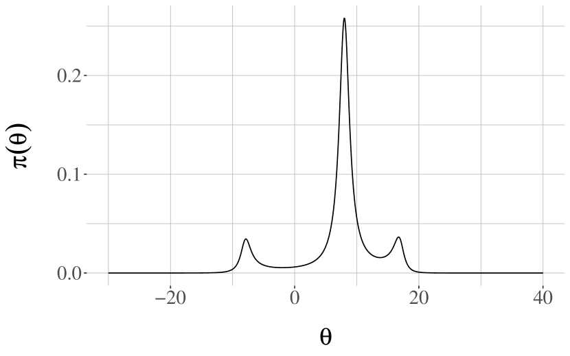
(a)

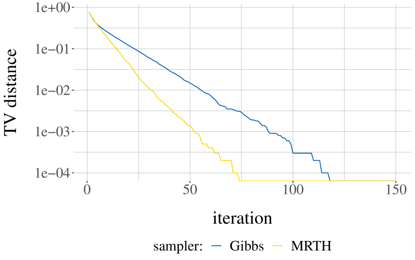
(b)

Figure 4.1: Cauchy-Normal example: target density (left) and upper bounds on $|\pi_{0}P^{t}-\pi|_{\text{TV}}$ for two algorithms (right).

The target is the posterior distribution in a Cauchy location model, with a Normal prior on the location parameter denoted by $\theta$. We observe $n=3$ measurements $z_{1}=-8,z_{2}=+8,z_{3}=+17$, assumed to be realizations of $\text{Cauchy}(\theta,1)$. The prior on $\theta$ is $\text{Normal}(0,100)$. We consider the test function $h:x\mapsto x$. The first algorithm considered here is the Gibbs sampler described in Robert (1995), alternating between Exponential and Normal draws:

$$\eta_{i}|\theta \sim\text{Exponential}\left(\frac{1+(\theta-z_{i})^{2}}{2}\right)\quad\forall i=1,\ldots,n,$$

$$\theta^{\prime}|\eta_{1},\ldots,\eta_{n} \sim\text{Normal}\left(\frac{\sum_{i=1}^{n}\eta_{i}z_{i}}{\sum_{i=1}^{n}\eta_{i}+\sigma^{-2}},\frac{1}{\sum_{i=1}^{n}\eta_{i}+\sigma^{-2}}\right),$$

where $\sigma^{2}=100$ is the prior variance. The coupling of this Gibbs sampler is done using common random numbers for the $\eta$-variables, and a maximal coupling for the update of $\theta$; see Appendix A.

We can show that Assumption 2 holds for all $\kappa$ for this coupled Gibbs sampler. Consider any pair $\theta$, $\tilde{\theta}$, and the pair of next values, $\theta^{\prime}$, $\tilde{\theta}^{\prime}$. Write $\eta$ and $\tilde{\eta}$ for the auxiliary variables in each chain. First observe that the means of the Normal distributions, being of the form

$$\frac{\sum_{i=1}^{n}\eta_{i}z_{i}}{\sum_{i=1}^{n}\eta_{i}+\sigma^{-2}}=\frac{\sum_{i=1}^{n}\eta_{i}z_{i}}{\sum_{i=1}^{n}\eta_{i}}\frac{\sum_{i=1}^{n}\eta_{i}}{\sum_{i=1}^{n}\eta_{i}+\sigma^{-2}},$$

takes values within $(-a,+a)$ with $a=\max|z_{i}|$, since it is a weighted average of $(z_{i})$ multiplied by a value in $(0,1)$. Therefore the mean of the next $\theta^{\prime}$ is within a finite interval that does not depend on the previous $\theta$. Regarding the variance $(\sum_{i=1}^{n}\eta_{i}+\sigma^{-2})^{-1}$, note that $\eta_{i}=-{2}/({1+(\theta-z_{i})^{2}})\log U_{i}$, where $U_{i}$ is Uniform$(0,1)$, thus $\eta_{i}\leq-2\log U_{i}$ and finally $(\sum_{i=1}^{n}\eta_{i}+\sigma^{-2})^{-1}\geq(\sigma^{-2}+\sum_{i=1}^{n}(-2\log U_{i}))^{-1}$. Also, $(\sum_{i=1}^{n}\eta_{i}+\sigma^{-2})^{-1}\leq\sigma^{2}$. The distribution of $\sum_{i=1}^{n}(-2\log U_{i})$ does not depend on $\theta$, thus we can define an interval $(c,d)\subset(0,\infty)$ and $\epsilon\in(0,1)$, independently of $\theta$ and $\tilde{\theta}$, such that $(\sum_{i=1}^{n}\eta_{i}+\sigma^{-2})^{-1}\in(c,d)$ and $(\sum_{i=1}^{n}\tilde{\eta}_{i}+\sigma^{-2})^{-1}\in(c,d)$ simultaneously with probability $\epsilon$.

Therefore, with probability $\epsilon$, the pair $(\theta^{\prime},\tilde{\theta}^{\prime})$ is drawn from a maximal coupling of two Normals, which means and variances are in finite intervals defined independently of $(\theta,\tilde{\theta})$. Two such Normals have a total variation distance that is bounded away from one, therefore there exists some $\delta>0$ such that, overall, $\mathbb{P}(\theta^{\prime}=\tilde{\theta}^{\prime}|\theta,\tilde{\theta})>\epsilon\delta$, for some $\epsilon>0$, $\delta>0$ and all $(\theta$,$\tilde{\theta})$. Therefore the meeting time has Geometric tails.

The second algorithm is a Metropolis–Rosenbluth–Teller–Hastings (MRTH) algorithm with Normal proposal, with standard deviation $10$. Its coupling employs a reflection-maximal coupling of the proposals. Verification of Assumption 2 can be done using Proposition 4 in Jacob et al. (2020). Indeed Jarner & Hansen (2000) describe a generic drift function for MRTH when the target is super-exponential: $\lim_{|x|\to\infty}(x/|x|)\nabla\log\pi(x)=-\infty$. This applies here because the prior is Normal and the likelihood is upper-bounded. We conclude that the meeting times have Geometric tails and thus Assumption 2 holds for any $\kappa>1$.

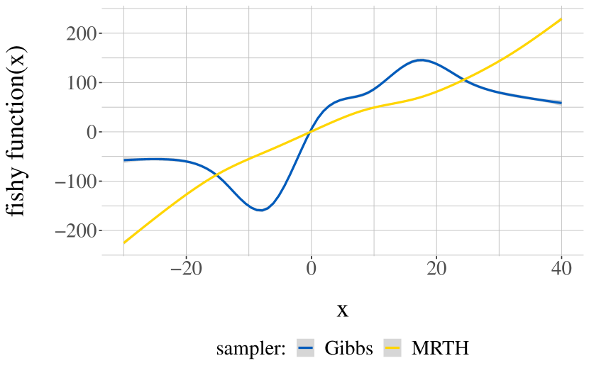
(a)

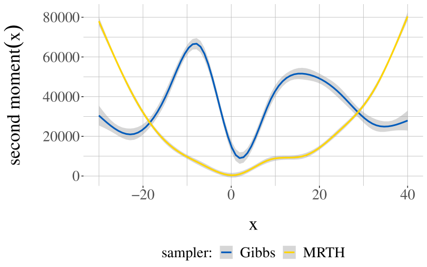
(b)

Figure 4.2: Cauchy-Normal example: estimation of $g(x)$ (left) and of second moment of the estimator, $\mathbb{E}[G(x)^{2}]$ (right).

The initial distribution, for both chains, is set to $\pi_{0}=\text{Normal}(0,1)$, for which one can verify that ${\rm d}\pi_{0}/{\rm d}\pi$ is bounded. Figure 4.1(a) shows the target density and Figure 4.1(b) provides upper bounds on $|\pi_{0}P^{t}-\pi|_{\text{TV}}$ for the two algorithms, using the method of Biswas et al. (2019). The state $y$ used to define $g=g_{y}$ in (2.3) is set to zero. Figure 4.2(a) shows the estimated fishy functions for the two algorithms, and Figure 4.2(b) shows the estimated second moments $\mathbb{E}[G(x)^{2}]$, for a grid of values of $x$ and using $10^{3}$ independent repeats of $G(x)$ for each $x$. Here the fishy functions $g$ are markedly different for both algorithms. If we interpret the fishy function as an indication of the asymptotic bias of MCMC as in Remark 13, we see that this bias diverges for MRTH whereas it seems uniformly bounded for the Gibbs sampler. Indeed by inspecting the updates of the Gibbs sampler, we note that if $|\theta|$ goes to infinity, the $\eta$-variables will be drawn from Exponential distributions with increasingly high rates, and in turn the next $\theta^{\prime}$ will be drawn from a Normal distribution with mean going to zero and variance going to $\sigma^{2}$. Thus the bias of estimators produced by the Gibbs sampler does not increase arbitrarily when the starting point diverges, as it does with the MRTH sampler.

From Figure 4.1(b) we select $k=100$, $L=100$ for the Gibbs sampler, and $k=75$, $L=75$ for MRTH. In both cases we use $\ell=5k$. We generate SUAVE estimators using different values of $R$, for both MCMC algorithms. We first use uniform selection probabilities, $\xi=1/N$. The results of $M=10^{3}$ independent runs are shown in Tables 4.1 and 4.2. Each entry shows a $95\%$ confidence interval obtained with the nonparametric bootstrap from the $M$ independent replications. The columns correspond to: 1) $R$: the number of atoms in each signed measure $\hat{\pi}$ at which fishy function estimators are generated, 2) estimate: overall estimate of $v(P,h)$, obtained by averaging $M=10^{3}$ independent estimates, 3) total cost of each proposed estimate, in units of “Markov transitions” 4) fishy cost: subcost associated with the fishy function estimates (increases with $R$), 5) empirical variance of the proposed estimators (decreases with $R$), and 6) inefficiency: product of variance and total cost (smaller is better). We observe that it is worth increasing $R$ up to the point where the fishy cost accounts for a significant portion of the total cost. From these tables we can confidently conclude that MRTH leads to a smaller asymptotic variance than the Gibbs sampler. Combined with an implementation-specific measure of the wall-clock time per iteration this can lead to a practical ranking of these two algorithms.

R	estimate	total cost	fishy cost	variance of estimator	inefficiency
1	[736 - 992]	[1049 - 1054]	[32 - 36]	[3e+06 - 6.4e+06]	[3.1e+09 - 6.7e+09]
10	[835 - 923]	[1349 - 1363]	[332 - 345]	[4.7e+05 - 5.9e+05]	[6.4e+08 - 8e+08]
50	[849 - 903]	[2686 - 2713]	[1667 - 1696]	[1.7e+05 - 2.1e+05]	[4.7e+08 - 5.6e+08]
100	[856 - 903]	[4379 - 4423]	[3361 - 3406]	[1.4e+05 - 1.7e+05]	[6.3e+08 - 7.4e+08]

Table 4.1: Cauchy-Normal example: estimators of $v(P,h)$ for the Gibbs sampler.

R	estimate	total cost	fishy cost	variance of estimator	inefficiency
1	[299 - 388]	[786 - 788]	[23 - 25]	[4e+05 - 7.3e+05]	[3.2e+08 - 5.8e+08]
10	[331 - 364]	[996 - 1003]	[233 - 240]	[6.2e+04 - 7.9e+04]	[6.3e+07 - 7.8e+07]
50	[333 - 351]	[1947 - 1966]	[1185 - 1203]	[1.9e+04 - 2.3e+04]	[3.8e+07 - 4.6e+07]
100	[335 - 349]	[3139 - 3168]	[2376 - 2405]	[1.3e+04 - 1.6e+04]	[4.2e+07 - 5e+07]

Table 4.2: Cauchy-Normal example: estimators of $v(P,h)$ for the MRTH sampler.

Using the fishy function estimates shown in Figure 4.2, we fit generalized additive models (Wood, 2017) with a cubic spline basis for the function $x\mapsto\mathbb{E}[{G}(x)^{2}]$ in order to approximate the optimal selection probabilities $\xi$ in (3.7). We then run the proposed estimators of $v(P,h)$, for both algorithms, with $R=10$ and $M=10^{3}$ independent replicates, using the approximated optimal $\xi$. The results are shown in Table 4.3. We report the fishy cost, and we note that it is impacted by the optimal tuning of selection probabilities: for Gibbs it increases, while for MRTH it decreases. The variance of the estimator decreases, as expected. Overall the inefficiency decreases by a factor of $2$ or $3$ in this example.

algorithm	selection $\xi$	fishy cost	variance of estimator	inefficiency
Gibbs	uniform	[332 - 345]	[4.7e+05 - 5.9e+05]	[6.4e+08 - 8e+08]
Gibbs	optimal	[408 - 422]	[2.2e+05 - 2.8e+05]	[3.1e+08 - 4e+08]
MRTH	uniform	[233 - 240]	[6.2e+04 - 7.8e+04]	[6.2e+07 - 7.8e+07]
MRTH	optimal	[190 - 196]	[2.2e+04 - 2.7e+04]	[2.1e+07 - 2.6e+07]

Table 4.3: Cauchy-Normal example: estimators of $v(P,h)$ for Gibbs and MRTH, using either optimal or uniform selection probabilities $\xi$.

4.2 Comparison with standard asymptotic variance estimators

We consider the autoregressive process $X_{t}=\phi X_{t-1}+W_{t}$, where $W_{t}\sim\text{Normal}(0,1)$, and $(W_{t})$ are independent. We set $\phi=0.99$. The initial distribution is $\pi_{0}=\text{Normal}(0,4^{2})$. The target distribution is $\text{Normal}(0,(1-\phi^{2})^{-1})$, and for $h:x\mapsto x$ the asymptotic variance is $v(P,h)=(1-\phi)^{-2}$. We use a reflection-maximal coupling to define the coupled kernel $\bar{P}$, see Appendix A. Appendix E verifies Assumption 2 for all $\kappa>1$. Figure 4.3(a) provides upper bounds on the TV distance to stationarity, and from this we will choose $k=500$, $L=250$, $\ell=5k$ for unbiased MCMC approximations in the sequel. The state $y\in\mathbb{X}=\mathbb{R}$, used to define $g=g_{y}$ in (2.3), is set as $y=0$. Figure 4.3(b) shows the estimated fishy function, from $100$ independent runs for a grid of values of $\phi$. We can calculate that $g_{y}$ here is the function $x\mapsto(1-\phi)^{-1}x$.

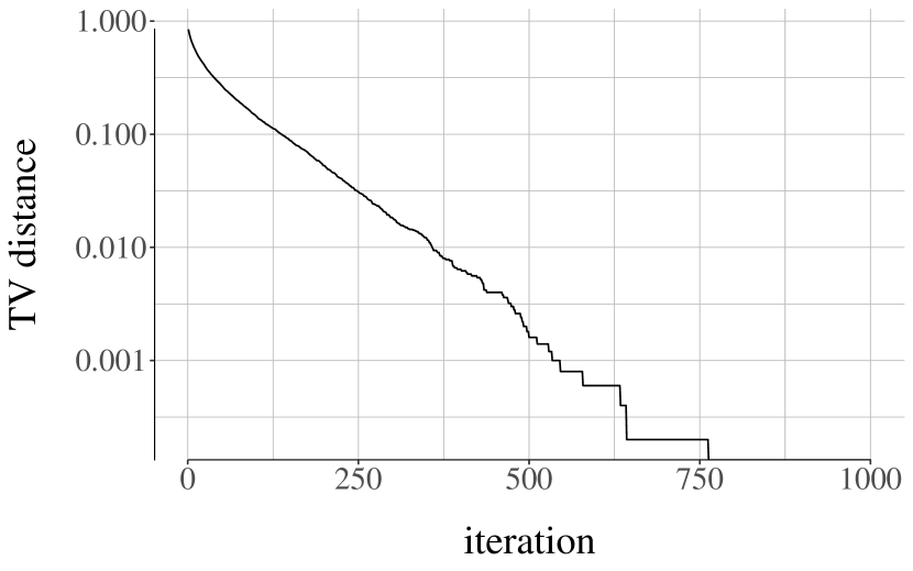
(a)

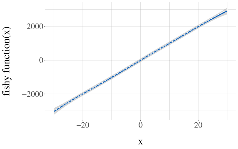
(b)

Figure 4.3: AR(1) example: upper bounds on $|\pi_{0}P^{t}-\pi|_{\text{TV}}$ (left), estimation of $g(x)$ (right) in full blue with exact $g$ in dashed white.

R	estimate	total cost	fishy cost	variance of estimator	inefficiency
1	[8178 - 10364]	[5234 - 5261]	[145 - 168]	[2.4e+08 - 4.8e+08]	[1.3e+12 - 2.5e+12]
10	[9414 - 10250]	[6676 - 6756]	[1585 - 1667]	[4e+07 - 5.5e+07]	[2.6e+11 - 3.7e+11]
50	[9748 - 10206]	[13148 - 13350]	[8069 - 8256]	[1.2e+07 - 1.5e+07]	[1.6e+11 - 2e+11]
100	[9840 - 10240]	[21259 - 21558]	[16163 - 16475]	[9.2e+06 - 1.1e+07]	[2e+11 - 2.4e+11]

Table 4.4: AR(1) example: unbiased estimation of the asymptotic variance $v(P,h)$. Here $v(P,h)=10^{4}$.

The performance of the proposed estimator of $v(P,h)$ is shown in Table 4.4. The columns are as in Tables 4.1 and 4.2 in the previous section. The results are based on $M=10^{3}$ independent replicates. We see that increasing $R$ improves the efficiency with diminishing returns. Overall we obtain accurate estimates of $v(P,h)$ with parallel runs that each costs of the order of $10^{4}$ iterations.

Next we compare the proposed estimator with the following “naive” strategy: generate a chain of length $T$ (post burn-in), compute the estimate $T^{-1}\sum_{t=0}^{T-1}h(X_{t})$, repeat $M$ times independently and compute the empirical variance of the $M$ estimates. We set $T=13,000$ to match the cost of our estimator with $R=50$. We find that the naive strategy has a bias (as $M\to\infty$) equal to $-77$, and an asymptotic variance of $2\times 10^{8}$. This is about 10 times larger than the variance of the proposed estimator reported in Table 4.4.

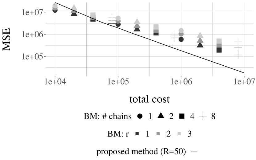
(a)

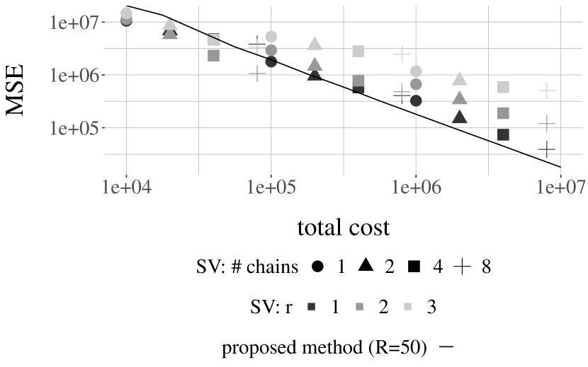
(b)

Figure 4.4: AR(1) example: mean squared error against total cost, for batch means (BM, left) and spectral variance (SV, right) estimators of $v(P,h)$. The performance of the proposed method (with $R=50$) is indicated with a full line.

We continue the comparison with two standard families of asymptotic variance estimators: “batch means” (BM) and “spectral variance” (SV) as implemented in the mcmcse package (Flegal et al., 2020). These estimators are based on batch sizes determined with the method of Liu et al. (2022). For each class of methods, we use three values of the lugsail parameter, $r\in\{1,2,3\}$. We compute these estimators of $v(P,h)$ using chains of lengths in $\{10^{4},10^{5},10^{6}\}$, and numbers of parallel chains in $\{1,2,4,8\}$. We base all the results on $400$ independent trajectories of length $10^{6}$, so for example we obtain $400$ independent estimators based on one chain, $200$ based on two chains, etc. For each configuration we approximate the mean squared error (MSE), and the total cost is equal to number of chains multiplied by the time horizon. Finally, we report the MSE that would be achieved by our proposed method, using $R=50$, if we generated sequentially a number of independent replicates of SUAVE corresponding to the given total cost. The comparison here does not account for any potential speed up on parallel architectures. The results are shown in Figure 4.4, where both axes are on logarithmic scale. Overall we note that our proposed method is competitive with standard asymptotic variance estimators. We also observe that the different estimators converge at different rates as a function of the total cost.

The experiments reported in Figure 4.4 suggest that if the practitioner’s interest lies in very cheap but not necessarily accurate estimators of $v(P,h)$, SUAVE appears worse than BM and SV, and furthermore SUAVE involves the extra effort of designing and implementing couplings. However for accurate estimates SUAVE appears valuable, particularly for practitioners with access to parallel processors.

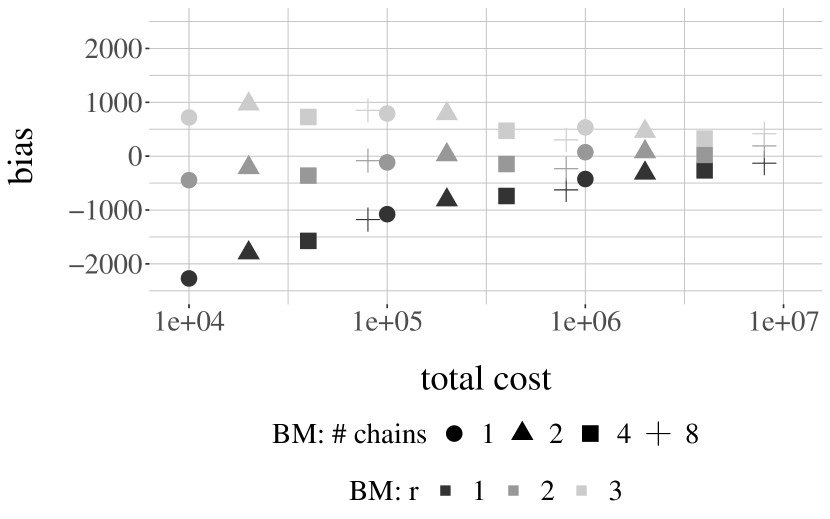
(a)

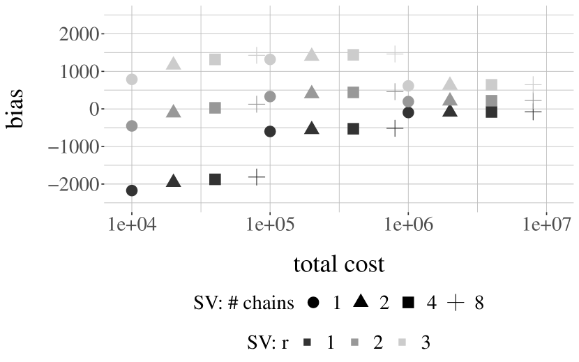
(b)

Figure 4.5: AR(1) example: bias against total cost, for batch means (BM, left) and spectral variance (SV, right) estimators of $v(P,h)$. The proposed method is, on the other hand, unbiased.

Finally we produce similar plots for the bias instead of the mean squared error, shown in Figure 4.5. The figure includes only batch means and spectral variance estimators since the proposed method is unbiased by design. We see that the $r$ lugsail parameter has a strong effect on the bias. In particular, the value $r=1$ that resulted in the smallest MSE in Figure 4.4 corresponds to a noticeable negative bias, that diminishes as the computing budget increases.

4.3 High-dimensional Bayesian linear regression

We examine a more challenging example, with a linear regression of $n=71$ responses on $p=4088$ predictors of the riboflavin data set (Bühlmann et al., 2014). The model, MCMC algorithm and its coupling are taken from Biswas et al. (2022) and a self-contained description is provided in Appendix C; essentially we use a shrinkage prior on the coefficients (e.g. Bhadra et al., 2019) and the target distribution is the posterior distribution of the regression coefficients, denoted by $\beta$, along with the global precision, the local precisions, and the variance of the observation noise. The state space is of dimension $2p+2=8178$. This example motivates the implementation of reservoir sampling to select the states at which to estimate the fishy function, as described in Section 3.3. In this example, the meeting times have been shown to have Exponential tails in Biswas et al. (2022, Proposition 6) under mild assumptions, so that Assumption 2 holds for any $\kappa$.

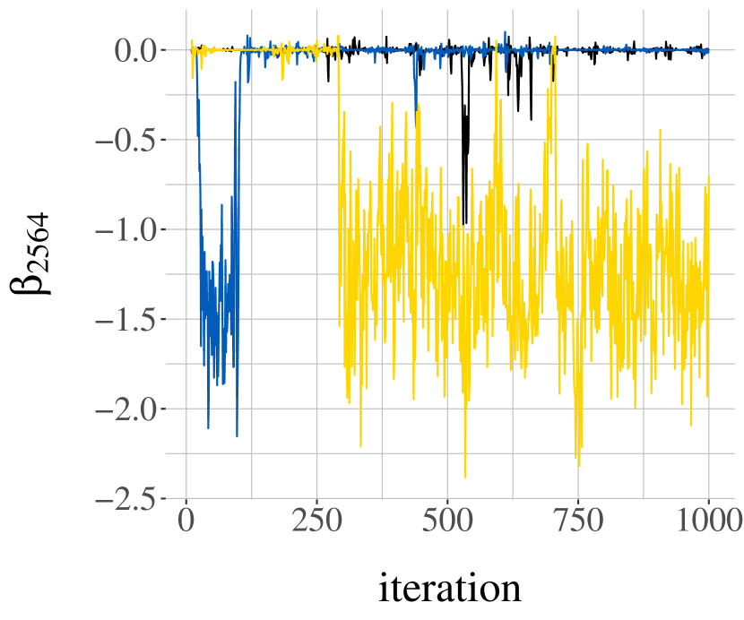
(a)

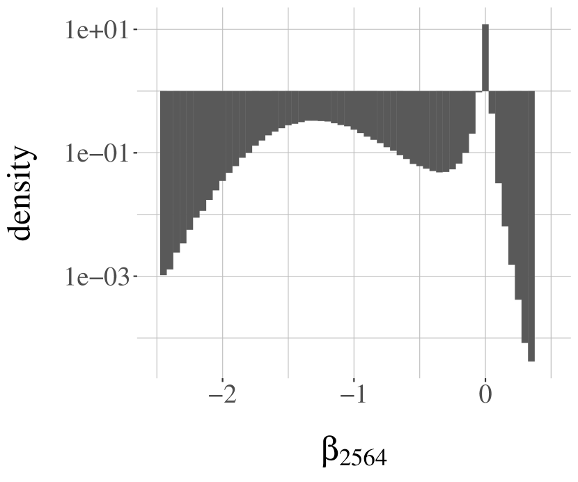
(b)

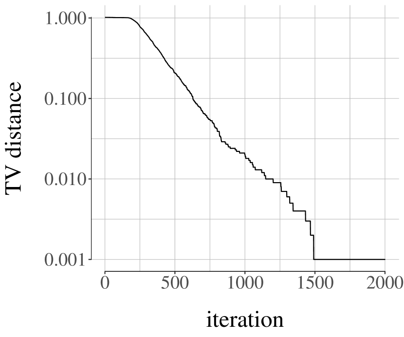
(c)

Figure 4.6: High-dimensional Bayesian linear regression example. Left: trace of the component $\beta_{2564}$ of three independent chains. Middle: histogram of $\beta_{2564}$, obtained from long MCMC runs, with $y$-axis on logarithmic scale. Right: upper bounds on $|\pi_{0}P^{t}-\pi|_{\text{TV}}$.

Based on preliminary runs, we choose the test function $h:x\mapsto\beta_{2564}$, which is a coordinate of the regression coefficients with a clearly bimodal marginal posterior distribution. Figure 4.6(a) shows three independent traces of $h(X_{t})$ over the first 1000 iterations. Figure 4.6(b) presents a histogram of $\beta_{2564}$, obtained from 10 independent chains run for 50,000 iterations each and discarding 2000 iterations as burn-in. Figure 4.6(c) shows upper bounds on $|\pi_{0}P^{t}-\pi|_{\text{TV}}$ obtained with the method of Biswas et al. (2019), using a lag $L=1000$ and $10^{3}$ independent meeting times. From this we choose $k=L=1000$ and $\ell=5k$.

To define $g=g_{y}$, we draw $y$ once from the prior, and keep it fixed. We generate $M=10^{3}$ independent estimates of $v(P,h)$, for $R\in\{1,5,10\}$. The results are summarized in Table 4.5. We again observe tangible gains in efficiency when increasing $R$, with diminishing returns. Overall we obtain relatively precise information about $v(P,h)$.

R	estimate	total cost	fishy cost	variance of estimator	inefficiency
1	[77 - 98]	[12310 - 12383]	[1522 - 1597]	[2.2e+04 - 3.3e+04]	[2.8e+08 - 4.1e+08]
5	[78 - 88]	[18466 - 18626]	[7687 - 7840]	[5.5e+03 - 6.9e+03]	[9.9e+07 - 1.3e+08]
10	[78 - 85]	[26225 - 26436]	[15437 - 15645]	[2.6e+03 - 3.1e+03]	[6.8e+07 - 8.2e+07]

Table 4.5: High-dimensional Bayesian linear regression example: proposed estimators of $v(P,h)$.

Next we illustrate the point made in Section 3.5 about the use of estimates of $v(P,h)$ to tune unbiased MCMC estimators. Here, with $k=500$, $L=500$ and $\ell=5k$, unbiased MCMC estimators of $\pi(h)$ have an expected cost of $5394$ and a variance of $0.020$, leading to an inefficiency of $106$. This is not much larger than the asymptotic variance $v(P,h)$, estimated to be around $80$. Users can then decide whether increasing the values of $k$, $L$ or $\ell$ is warranted.

4.4 Particle marginal Metropolis–Hastings

We consider the state space model (SSM) example in Middleton et al. (Section 4.2 2020), inspired by a model capturing the activation of neuron of rats when responding to a periodic stimulus. The observations are counts of neuron activations over $50$ experiments. We consider $100$ data points represented in Figure 4.7(a). They are modelled as

$$y_{t}|x_{t}\sim\text{Binomial}(50,\text{logistic}(x_{t})),$$

where $\text{logistic}:x\mapsto 1/(1+\exp(-x))$ and

$$x_{0}\sim\text{Normal}(0,1),\quad\text{and}\quad\forall t\geq 1\quad x_{t}|x_{t-1}\sim\text{Normal}(\alpha x_{t-1},\sigma^{2}).$$

The prior is $\text{Uniform}(0,1)$ on $\alpha$, and $\sigma^{2}$ is fixed to 1.5 here for simplicity. The likelihood is intractable but can be estimated using a particle filter. As in Middleton et al. (2020) we use controlled SMC (Heng et al., 2020), and we plug the likelihood estimator in the particle marginal Metropolis–Hastings algorithms (PMMH, Andrieu et al., 2010). We use 3 iterations of controlled SMC at each PMMH iteration. The proposal on $\alpha$ is a Normal random walk, with a standard deviation drawn from $\text{Uniform}(0.001,0.2)$ at each iteration. The coupling operates with a reflection-maximal coupling of the proposals, and independent runs of SMC if the proposals differ. Formal verification of Assumption 2 is difficult, but relevant elements can be found in Middleton et al. (2020, Section 2.3). We initialize the chains from the prior $\text{Uniform}(0,1)$. An approximation of the posterior distribution is shown in Figure 4.7(b), obtained from 14 chains of length $10,000$ and a burn-in of $1000$ steps.

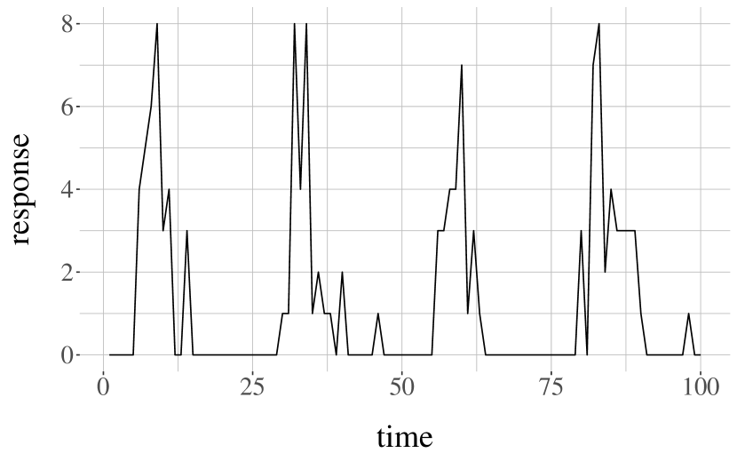
(a)

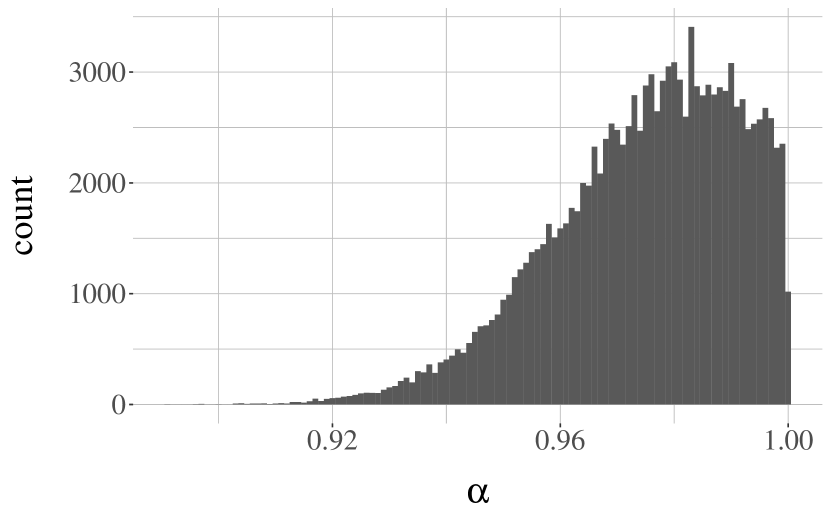
(b)

Figure 4.7: SSM example: 100 observations (left) and posterior distribution on $\alpha$ (right) approximated with particle marginal Metropolis–Hastings.

Expecting PMMH to be polynomially ergodic, we examine the tails of the distribution of the meeting times. We generate $10^{5}$ meeting times, either using 64 or 256 particles in each run of SMC within PMMH. The empirical survival functions of the meeting times $\tau$, or more exactly of $\tau-L$ with a lag $L=100$, are shown in Figure 4.8. Since both axes are on logarithmic scale, a straight line indicates a polynomial decay for $\mathbb{P}(\tau>t)$. We indeed observe straight lines on the parts of figure where $t$ is large enough. Using linear regression we estimate the polynomial rate to be around 1 when using 64 particles (focusing on $t>200$), and above 2 when using 256 particles (focusing on $t>100$).

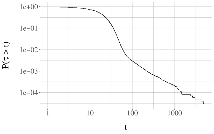
(a)

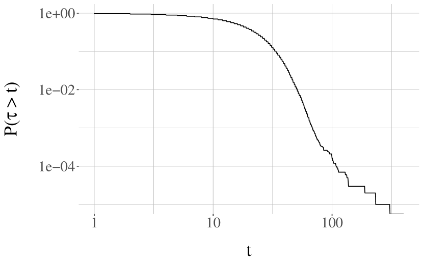
(b)

Figure 4.8: SSM example: survival function $\mathbb{P}(\tau>t)$ when using 64 particles (left) or 256 particles (right) in PMMH. Both axes use logarithmic scale.

Given the heavy tails of $\tau$ when using 64 particles, we were not able to reliably estimate the associated $v(P,h)$. We thus focus on the use of 256 particles, and we generate SUAVE to estimate $v(P,h)$, $M=500$ times independently, for $h:x\mapsto x$. We set $y=0.5$ in the definition of the fishy function estimator $G_{y}$. We use $k=L=500$ and $\ell=5k$ for unbiased MCMC approximations. We choose $R=50$, the number of atoms at which $g_{y}$ is estimated per signed measure. From the SUAVE runs, we can extract all the locations at which $g_{y}$ is estimated by $G_{y}$, along with the estimates. We then represent an approximation of $g_{y}$ in Figure 4.9(a), and a histogram of the $500$ estimates of $v(P,h)$ in Figure 4.9(b). We see that the relative variance is fairly large, and notice that many estimates are negative.

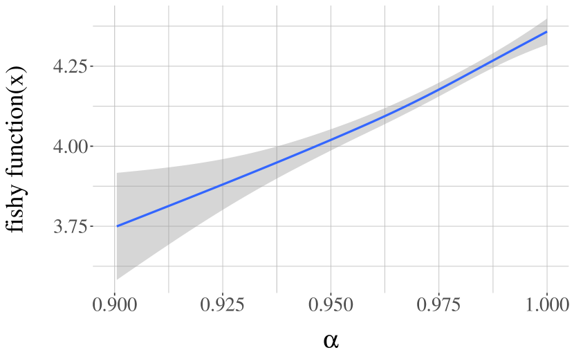
(a)

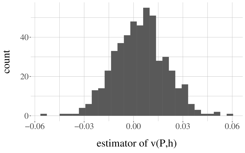
(b)

Figure 4.9: SSM example: using $y=0.5$, estimation of $g_{y}(x)$ (left) and histogram of proposed estimators of $v(P,h)$ (right).

We then change $y$ from $0.5$ to $0.975$, i.e. we place $y$ in the middle of the posterior distribution as shown in Figure 4.7(b), and reproduce the same plots in Figure 4.10. We see that the fishy function takes smaller values and its estimation is more precise. As a result, the distribution of $\hat{v}(P,h)$ is considerably more concentrated. The effect of the choice of $y$ is summarized in Table 4.6, where all entries are confidence intervals based on the nonparametric bootstrap. We observe that the choice of $y$ impacts the cost of fishy function estimation, as well as its variance and thus the variance of SUAVE. Here this results in orders of magnitude of difference in efficiency.

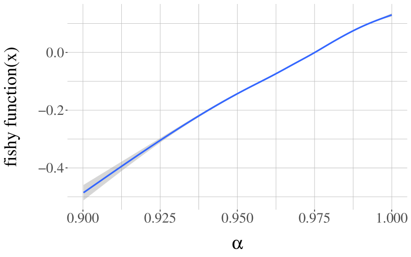
(a)

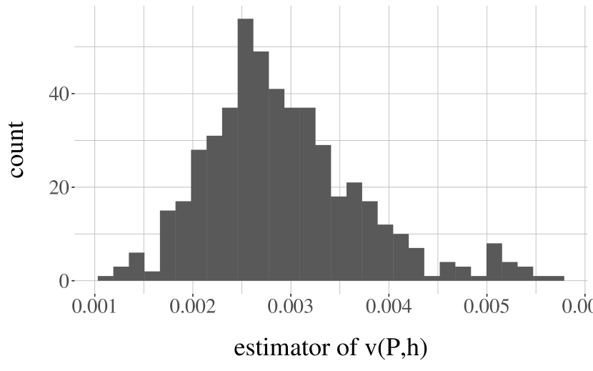
(b)

Figure 4.10: SSM example: using $y=0.975$, estimation of $g_{y}(x)$ (left) and histogram of proposed estimators of $v(P,h)$ (right).

y	estimate	fishy cost	variance of estimator	inefficiency
0.5	[2.64e-03 - 5.32e-03]	[3.62e+03 - 3.67e+03]	[2.2e-04 - 2.8e-04]	[1.9e+00 - 2.5e+00]
0.975	[2.85e-03 - 2.99e-03]	[1.01e+03 - 1.05e+03]	[5.4e-07 - 7.4e-07]	[3.3e-03 - 4.5e-03]

Table 4.6: SSM example: effect of $y$ on the proposed confidence interval for $v(P,h)$, the cost of fishy function estimation, the variance of $\hat{v}(P,h)$ and its inefficiency, based on $M=500$ independent repeats, and using $R=50$, $k=L=500$, $\ell=5k$.

Finally we can compare $v(P,h)\approx 2.9\times 10^{-3}$ to the inefficiency associated with unbiased MCMC, here with $k=L=500$ and $\ell=5k$. We compute the variance and the expected cost of unbiased MCMC estimators of $\pi(h)$ and find an inefficiency of $3.8\times 10^{-3}$, so the loss of efficiency of unbiased MCMC relative to standard MCMC is approximately $30\%$.

5 Discussion

When a Markov chain admits an accessible atom $\alpha$, a solution of the Poisson equation (e.g. Glynn & Meyn, 1996) is $g(x)=\mathbb{E}_{x}\left[\sum_{k=0}^{\sigma_{\alpha}}h_{0}(X_{k})\right]$, where $\sigma_{\alpha}=\inf\{n\geq 0:X_{n}\in\alpha\}$. This allows approximation of $g$ pointwise by simulation if one can identify entries into $\alpha$ and one can approximate $h_{0}=h-\pi(h)$ pointwise. The approach we took in this article is different in that it does not rely on identifying atoms, and hence may be applicable in scenarios where this regenerative approximation is not implementable. For example, proper atoms may not exist for a given general state space Markov chain, and identification of hitting times of an atom for a suitable split chain as in Mykland et al. (1995) is not always feasible. While it is often possible to define a modified Markov chain that admits an easily identified, accessible atom (Brockwell & Kadane, 2005; Lee et al., 2014), the corresponding solution of the Poisson equation may not be similar to that of the original chain. Note also that, when atoms can be identified, one would often use regenerative simulation to approximate the asymptotic variance (Hobert et al., 2002), which can be expressed as $v(P,h)=\pi(\alpha)\mathbb{E}_{\alpha}\left[\left\{\sum_{k=1}^{\tau_{\alpha}}h_{0}(X_{k})\right\}^{2}\right]$ (see, e.g., Bednorz et al., 2008).

Coupling techniques have been extensively used to study distances between a Markov chain at time $t$ and its limiting distribution. Couplings yield upper bounds on these distances and on the resulting mixing time, and these bounds are rarely sharp. Therefore, without matching lower bounds, coupling techniques cannot determine whether an algorithm converges faster than another. On the other hand, the proposed coupling-based asymptotic variance estimators are unbiased, even with sub-optimal couplings, under conditions presented in this article. Thus, with sufficient computing resources we can determine which algorithm leads to the smallest asymptotic variance.

Our experiments suggest that the proposed estimators of $v(P,h)$ are practical and competitive. They only apply to settings where the requisite couplings are available, so that the proposed methods demand more from the user, compared to batch means and spectral methods. On the other hand, the proposed estimators are unbiased, with the important consequence that averages of independent copies achieves the Monte Carlo rate of convergence. This compares favourably to batch means estimators, for which, under general assumptions, convergence occurs at rate $\sqrt{a_{n}}$, where $a_{n}$ is the number of batches, and $a_{n}$ is often chosen as $a_{n}=n^{1/2}$ or $a_{n}=n^{2/3}$ where $n$ is the length of the chain (see Theorem 2.1, Chakraborty et al., 2022).

As with other works on unbiased MCMC, it is worth emphasizing that the performance depends on both the MCMC algorithm under consideration, its initialization and its coupling. We refer to the bimodal target in Section 5.1 of Jacob et al. (2020) for a situation where multimodality in the target distribution combined with a poor design of the MCMC sampler gives misleading estimates in finite samples, despite the lack of bias and the finite variance. In our theoretical results, we have prioritized assumptions on the moments of meeting times of the coupled Markov chains under strong but reasonable initialization assumptions, which can be cleanly separated from assumptions on the moments of functions. Given this emphasis, the results appear to be fairly strong and provide a sensible relationship between the moments of the meeting time and of moments of estimators. In applications, however, obtaining a precise estimate of the largest $\kappa$ in Assumption 2 is not straightforward and in many ways is similar to obtaining non-asymptotic convergence bounds for Markov chains.

Appendix A contains reminders on practical couplings of MCMC algorithms, Appendix B contains reminders on unbiased MCMC, Appendix C provides details on the Gibbs sampler for high-dimensional Bayesian regression employed in Section 4.3, Appendix D contains proofs of our main results, and Appendix E verifies Assumption 2 for the AR(1) process considered in Section 4.2. Code to reproduce the figures of this article can be found at: https://github.com/pierrejacob/unbiasedpoisson/.

Acknowledgments.

Research of AL supported by EPSRC grant ‘CoSInES (COmputational Statistical INference for Engineering and Security)’ (EP/R034710/1). Research of DV supported by SERB (SPG/2021/001322).

Appendix A Coupling of MCMC algorithms

For completeness we recall some implementable coupling techniques for MCMC. We focus on Metropolis–Rosenbluth–Teller–Hastings (MRTH) algorithms (Metropolis et al. 1953, Hastings 1970). The goal is to couple generated trajectories such that exact meetings can occur. Various relevant considerations are presented in Jacob et al. (2020), Wang et al. (2021).

Algorithm A.1 describes a simple way of coupling $P(X,\cdot)$ and $P(Y,\cdot)$ where $P$ is the transition associated with MRTH, with proposal transition $q$ and acceptance rate $\alpha_{\text{MRTH}}$. In the algorithmic description, a maximal coupling of two distributions $\mu$ and $\nu$ for random variables $X$ and $Y$, respectively, refers to a joint distribution $\gamma$ for $(X,Y)$ with marginals $\mu$ and $\nu$, and such that $\mathbb{P}(X=Y)$ is maximized over all such joint distributions; examples are provided below.

1. Sample $(X^{\star},Y^{\star})$ from a maximal coupling of $q(X,\cdot)$ and $q(Y,\cdot)$.

2. Sample $U\sim\text{Uniform}(0,1)$.

3. If $U<\alpha_{\text{MRTH}}(X,X^{\star})$, set $X^{\prime}=X^{\star}$, otherwise $X^{\prime}=X$.

4. If $U<\alpha_{\text{MRTH}}(Y,Y^{\star})$, set $Y^{\prime}=Y^{\star}$, otherwise $Y^{\prime}=Y$.

5. Return $(X^{\prime},Y^{\prime})$.

Algorithm A.1 A coupled Metropolis–Rosenbluth–Teller–Hastings kernel

Next we provide details on how to sample from maximal couplings of $q(x,\cdot)$ and $q(y,\cdot)$. A possibility, mentioned in Section 4.5 of Thorisson (2000), and called $\gamma$-coupling in Johnson (1998), is described in Algorithm A.2. The algorithm requires the ability to sample from $\mu$ and $\nu$. The cost of executing Algorithm A.2 is random, its expectation is independent of $\mu$ and $\nu$, and its variance goes to infinity as $|\mu-\nu|_{\text{TV}}\to 0$. A variant of the algorithm for which the variance is bounded for all $\mu,\nu$ is described in Gerber & Lee (2020).

1. Sample $X\sim\mu$.

2. Sample $W\sim\text{Uniform}(0,1)$.

3. If $W\leq\nu(X)/\mu(X)$, set $Y=X$.

4. Otherwise, sample $Y^{\star}\sim\nu$ and $W^{\star}\sim\text{Uniform}(0,1)$
   until $W^{\star}>\mu(Y^{\star})/\nu(Y^{\star})$, and set $Y=Y^{\star}$.

5. Return $(X,Y)$.

Algorithm A.2 Sampling from a maximal coupling of $\mu$ and $\nu$.

When $\mu$ and $\nu$ are Normal distributions with the same variance, an alternative maximal coupling procedure is described in Algorithm A.3; it was proposed in Bou-Rabee et al. (2020). Its cost is deterministic and independent of $\mu$ and $\nu$. In the algorithmic description, $\varphi$ refers to the probability density function of the standard Normal distribution.

1. Let $z=\Sigma^{-1/2}(\mu_{1}-\mu_{2})$ and $e=z/|z|$.

2. Sample $\dot{X}\sim\mathcal{N}(0_{d},I_{d})$, and $W\sim\text{Uniform}(0,1)$.

3. If $\varphi(\dot{X})W\leq\varphi(\dot{X}+z)$, set $\dot{Y}=\dot{X}+z$; else set $\dot{Y}=\dot{X}-2(e^{T}\dot{X})e$.

4. Set $X=\Sigma^{1/2}\dot{X}+\mu_{1},Y=\Sigma^{1/2}\dot{Y}+\mu_{2}$, and return $(X,Y)$.

Algorithm A.3 Reflection-maximal coupling of $\text{Normal}(\mu_{1},\Sigma)$ and $\text{Normal}(\mu_{2},\Sigma)$.

In the case of univariate Normal distributions $\text{Normal}(\mu_{1},\sigma^{2})$ and $\text{Normal}(\mu_{2},\sigma^{2})$, the procedure simplifies to Algorithm A.4. We used Algorithm A.4 to couple AR(1) processes in Section 4.2.

1. Let $z=(\mu_{1}-\mu_{2})/\sigma$.

2. Sample $\dot{X}\sim\text{Normal}(0,1)$, and $W\sim\text{Uniform}(0,1)$.

3. Set $X=\mu_{1}+\sigma\dot{X}$.

4. If $W<\varphi(z+\dot{X})/\varphi(\dot{X})$, set $Y=X$; else set $Y=\mu_{2}-\sigma\dot{X}$.

5. Return $(X,Y)$.

Algorithm A.4 Reflection-maximal coupling of (univariate) $\text{Normal}(\mu_{1},\sigma^{2})$ and $\text{Normal}(\mu_{2},\sigma^{2})$.

Beyond MRTH, various MCMC algorithms can be coupled so as to trigger exact meetings, for example Hamiltonian Monte Carlo (Heng & Jacob 2019, Xu et al. 2021), Gibbs samplers to sample partitions (Nguyen et al. 2022), or samplers for phylogenetic inference (Kelly et al. 2023). However there is no automatic recipe to construct efficient couplings, and it remains a task to solve on a “per-algorithm” basis.

Appendix B Unbiased MCMC estimators

B.1 Unbiased estimators of expectations and signed measures

Glynn & Rhee (2014) show how coupled Markov chains can be employed to construct unbiased estimators of stationary expectations. These estimators were considered in the Monte Carlo setting by Agapiou et al. (2018). We recall here the variations presented in Jacob et al. (2020) and follow-up works, that rely on a coupled Markov kernel $\bar{P}$ that induces meetings of the two chains. This removes the need to specify a truncation variable as in Glynn & Rhee (2014) and Agapiou et al. (2018).

Specifically, we construct the chains with a time lag $L\in\mathbb{N}$, which is a tuning parameter. The construction is as in Algorithm 2.1. We also introduce a “starting time” $k\in\mathbb{N}$, a “prospective end time” $\ell$, with $k\leq\ell$, which are tuning parameters. Under assumptions provided in Section D.4 (see also Jacob et al. 2020, Middleton et al. 2020), the following random variable is an unbiased estimator of $\pi(h)$:

$$H_{k}^{(L)}=h(X_{k})+\sum_{j=1}^{\infty}\{h(X_{k+jL})-h(Y_{k+(j-1)L})\}.$$ (B.1)

Consider a range of integers $k,\ldots,\ell$ for $k\leq\ell$ and associated estimators $H_{k}^{(L)},\ldots,H_{\ell}^{(L)}$ obtained from the same trajectories $(X_{t},Y_{t})_{t\geq 0}$. All of these estimators $(H_{t}^{(L)})_{t=k}^{\ell}$ are unbiased, so their average is unbiased and reads

$$H_{k:\ell}^{(L)} =\frac{1}{\ell-k+1}\sum_{t=k}^{\ell}H_{t}^{(L)}$$

$$=\frac{1}{\ell-k+1}\sum_{t=k}^{\ell}h(X_{t})+\frac{1}{\ell-k+1}\sum_{s=k}^{\ell}\sum_{j=1}^{\infty}\{h(X_{s+jL})-h(Y_{s+(j-1)L})\}.$$

We can find a simpler representation for the double sum in the above equation. Denote by $v_{t}$ the number of times that the term $\Delta_{t}=h(X_{t})-h(Y_{t-L})$ appears in the double sum. Then $v_{t}$ is the number of terms of the form $s+jL$ equal to $t$ as $s$ moves in $\{k,\ldots,\ell\}$ and $j\geq 1$. We can focus on $t$ in $\{k+L,\ldots,\tau-1\}$ since $v_{t}=0$ for $t$ outside of that range. Note that, for a given $s$, there can be at most one value of $j$ such that $s+jL=t$. So

$$v_{t}=|\{s\in\{k,\ldots,\ell\}:\exists j\geq 1:s+jL=t\}|.$$

We can re-write this as

$$v_{t}=|\{n\in\{t-\ell,\ldots,t-k\}:\frac{n}{L}\in\mathbb{Z}^{+}\}|,$$

where $\mathbb{Z}^{+}$ is the set of positive integers. In other words we are counting the positive multiples of $L$ within the range $\{t-\ell,\ldots,t-k\}$, for any $t\geq k+L$. We can restrict that range to $\{\max(L,t-\ell),\ldots,t-k\}$, since we cannot find a positive multiple of $L$ smaller than $L$. Now the range is between two positive integers. This yields:

$$v_{t}=\lfloor(t-k)/L\rfloor-\lceil\max(L,t-\ell)/L\rceil+1.$$ (B.2)

Indeed for two positive integers $a\leq b$, the number of multiples of $L$ within $\{a,\ldots,b\}$ is $\lfloor b/L\rfloor-\lceil a/L\rceil+1$.

Thus we obtain

$$H_{k:\ell}^{(L)}=\frac{1}{\ell-k+1}\sum_{t=k}^{\ell}h(X_{t})+\text{BC}_{k:\ell}^{(L)},$$ (B.3)

where $\text{BC}_{k:\ell}^{(L)}$ refers to a “bias cancellation” term,

$$\text{BC}_{k:\ell}^{(L)}=\sum_{t=k+L}^{\tau^{(L)}-1}\frac{v_{t}}{\ell-k+1}\left\{h(X_{t})-h(Y_{t-L})\right\}.$$ (B.4)

Instead of the above expressions that involve a test function $h$, we can consider the signed measure

$$\hat{\pi}({\rm d}x)=\frac{1}{\ell-k+1}\sum_{t=k}^{\ell}\delta_{X_{t}}({\rm d}x)+\sum_{t=k+L}^{\tau^{(L)}-1}\frac{v_{t}}{\ell-k+1}\left\{\delta_{X_{t}}-\delta_{Y_{t-L}}\right\}({\rm d}x),$$ (B.5)

as an unbiased approximation of $\pi$. This is of the form

$$\hat{\pi}({\rm d}x)=\sum_{n=1}^{N}\omega_{n}\delta_{Z_{n}}({\rm d}x),$$ (B.6)

where $N=\max(0,\tau^{(L)}-(k+L))+(\ell-k+1)$, $Z_{n}$ are states from either $(X_{t})$ or $(Y_{t})$ and $\omega_{t}$ are either $(\ell-k+1)^{-1}$, or of the form $\pm v_{t}(\ell-k+1)^{-1}$; in particular the weights can be negative.

If we count the cost of sampling from the kernel $P$ as one unit, and the cost of sampling from $\bar{P}$ as one unit if the chains have met already, and two units otherwise, then the random cost of obtaining (B.3), or (B.5), equals $\max(L,\ell+L-\tau^{(L)})+2(\tau^{(L)}-L)$ units.

The above unbiased estimators are to be generated independently in parallel, and averaged to obtain a final approximation of $\pi$. Since they are unbiased, the mean squared error is equal to the variance. To compare unbiased estimators with different cost, e.g. to compare different configurations of the tuning parameters $k,\ell,L$, we can compute the asymptotic inefficiency defined as the expected cost multiplied by the variance, as described in Glynn & Whitt (1992); the lower value, the better.

B.2 Upper bounds on the distance to stationarity

A by-product of the above estimator is an upper bound on $|\pi_{t}-\pi|_{\text{TV}}$ (Jacob et al. 2020, Biswas et al. 2019, Craiu & Meng 2022), given by

$$|\pi_{t}-\pi|_{\text{TV}}\leq\mathbb{E}\left[\max\left(0,\left\lceil\frac{\tau^{(L)}-L-t}{L}\right\rceil\right)\right].$$ (B.7)

The upper bound can be estimated using independent replications of the meeting time $\tau^{(L)}$. To justify (B.7), first use the triangle inequality to write

$$|\pi_{t}-\pi|_{\text{TV}} \leq\sum_{j=1}^{\infty}|\pi_{t+jL}-\pi_{t+(j-1)L}|_{\text{TV}}$$

$$\leq\sum_{j=1}^{\infty}\mathbb{P}(X_{t+jL}\neq Y_{t+(j-1)L})$$

$$=\sum_{j=1}^{\infty}\mathbb{P}(\tau^{(L)}>t+jL),$$

where the second inequality comes from the employed coupling being sub-optimal, and in the last line $\tau^{(L)}$ is defined as $\inf\{t\geq 1:X_{t}=Y_{t-L}\}$. By writing $\mathbb{P}(\tau^{(L)}>t+jL)=\mathbb{E}[\mathds{1}(\tau^{(L)}>t+jL)]$, and interchanging the infinite sum and the expectation, we obtain

$$|\pi_{t}-\pi|_{\text{TV}} \leq\mathbb{E}\left[\sum_{j=1}^{\infty}\mathds{1}(\tau^{(L)}>t+jL)\right]$$

$$=\mathbb{E}\left[|\{j\in\mathbb{Z}^{+}:jL<\tau^{(L)}-t\}|\right].$$

Recall that $\mathbb{Z}^{+}=\{1,2,\ldots\}$. If $\tau^{(L)}-t\leq L$ then the set in the above display is empty. If $\tau^{(L)}-t>L$, then the set has cardinality equal to the number of multiples of $L$ within the range $\{L,\ldots,\tau^{(L)}-t-1\}$. Using the same formula as before this is $\lfloor(\tau^{(L)}-t-1)/L\rfloor-\lceil L/L\rceil+1$. Finally we observe that $\lfloor(\tau^{(L)}-t-1)/L\rfloor$ and $\lceil(\tau^{(L)}-t-L)/L\rceil$ are identical when $\tau^{(L)}-t>L$, which can be seen by considering the cases: $(\tau^{(L)}-t)/L\in\mathbb{N}$ and $(\tau^{(L)}-t)/L\notin\mathbb{N}$ separately. Thus we retrieve (B.7).

Appendix C MCMC for Bayesian linear regression with shrinkage prior

We provide details for the numerical experiments of Section 4.3. The example is taken from Biswas et al. (2022), where the authors consider couplings of the Gibbs sampler of Johndrow et al. (2020). We provide here a short and self-contained description of one particular version of the Gibbs sampler and its coupling; many more algorithmic considerations can be found in Biswas et al. (2022).

C.1 Model

The context is that of linear regression, with $n$ individuals and $p$ covariates, with $p\gg n$. The generative model is described below, where $Y$ is the outcome, $X$ the vector of explanatory variables, $\beta\in\mathbb{R}^{p}$ the regression coefficients, $\sigma^{2}\in\mathbb{R}_{+}$ the observation noise, $\xi$ is called the global precision and $\eta_{j}$ is the local precision associated with $\beta_{j}$ for $j\in\{1,\ldots,p\}$,

$$Y\sim\text{Normal}(X\beta,\sigma^{2}I_{n}),$$

$$\sigma^{2}\sim\text{InverseGamma}(a_{0}/2,b_{0}/2),$$

$$\xi^{-1/2}\sim\text{Cauchy}(0,1)^{+},$$

$$\text{for }j=1,\ldots,p\quad \beta_{j}\sim\text{Normal}(0,\sigma^{2}/\xi\eta_{j}),\quad\eta_{j}^{-1/2}\sim t(\nu)^{+}.$$

The distribution $t(\nu)^{+}$ refers to the Student t-distribution with $\nu$ degrees of freedom, truncated on $(0,\infty)$, with density $x\mapsto(1+x^{2}/\nu)^{-(\nu+1)/2}\mathds{1}(x\in(0,\infty))$ up to a multiplicative constant. The hyper-parameters are set as $a_{0}=1,b_{0}=1,\nu=2$. In our experiments we initialize Markov chains from the prior distribution.

C.2 Gibbs sampler

The main steps of the Gibbs sampler under consideration are as follows.

• For $j=1,\ldots,p$, sample each $\eta_{j}$ given $\beta,\xi,\sigma^{2}$ using slice sampling.

• Given $\eta$, sample $\beta,\xi,\sigma^{2}$:

  • $\xi$ given $\eta$ using an MRTH step,

  • $\sigma^{2}$ given $\eta,\xi$ from an Inverse Gamma distribution,

  • $\beta$ given $\eta,\xi,\sigma^{2}$ from a p-dimensional Normal distribution.

Overall the computational complexity is of the order of $n^{2}p$ operations per iteration, therefore it can be used with large $p$ and moderate values of $n$. Details on each step can be found below.

$\eta$-update.

The conditional distribution of $\eta$ given the rest has density

$$\pi(\eta|\beta,\sigma^{2},\xi)\propto\prod_{j=1}^{p}\frac{e^{-m_{j}\eta_{j}}}{\eta_{j}^{\frac{1-\nu}{2}}(1+\nu\eta_{j})^{\frac{\nu+1}{2}}}\quad\text{ where }m_{j}=\frac{\xi\beta_{j}^{2}}{2\sigma^{2}},$$

which we can target with the slice sampler described in Algorithm C.1, applied independently component-wise.

1. Sample $V\sim\text{Uniform}(0,1)$.

2. Sample $U_{j}|\eta_{j}\sim\text{Uniform}(0,(1+\nu\eta_{j})^{-\frac{\nu+1}{2}})$ by setting $U_{j}=V\times(1+\nu\eta_{j})^{-\frac{\nu+1}{2}}$.

3. Sample $\eta_{j}|U_{j}$ from the distribution with unnormalized density $\eta_{j}\mapsto\eta_{j}^{s-1}e^{-m_{j}\eta_{j}}$ on $(0,T_{j})$, with $T_{j}=(U_{j}^{-2/(1+\nu)}-1)/\nu$ and $s=(1+\nu)/2$. This can be done by sampling $U^{*}\sim\text{Uniform}(0,1)$ and setting

   $$\eta_{j}=\frac{1}{m_{j}}\gamma_{s}^{-1}\left(\gamma_{s}(m_{j}T_{j})U^{*}\right),$$

   where $\gamma_{s}(x):=\Gamma(s)^{-1}\int_{0}^{x}t^{s-1}e^{-t}dt\in[0,1]$ is the cdf of the $\mathrm{Gamma}(s,1)$ distribution.

Algorithm C.1 Iteration of slice sampling targeting $\eta_{j}\mapsto(\eta_{j}^{\frac{1-\nu}{2}}(1+\nu\eta_{j})^{\frac{\nu+1}{2}})^{-1}e^{-m_{j}\eta_{j}}$ on $(0,\infty)$.

$\xi$-update.

The conditional distribution of $\xi$ given $\eta$ has density

$$\pi(\xi|\eta\propto L(y|\xi,\eta)\pi_{\xi}(\xi),$$

where $L(y|\xi,\eta)$ is the marginal likelihood of the observations given $\xi$ and $\eta$, and $\pi_{\xi}$ is the prior density for $\xi$. We sample $\xi|\eta$ using a Metropolis–Rosenbluth–Teller–Hastings scheme. Given the current value of $\xi$, propose $\log(\xi^{*})\sim\text{Normal}(\log(\xi),\sigma_{\text{MRTH}}^{2})$, where we set $\sigma_{\text{MRTH}}=0.8$. Then calculate the ratio

$$q=\frac{L(y|\xi^{*},\eta)\pi_{\xi}(\xi^{*})\xi^{*}}{L(y|\xi,\eta)\pi_{\xi}(\xi)\xi},$$

using

$$\log(L(y|\xi,\eta))=-\frac{1}{2}\log(|M_{\xi,\eta}|)-\frac{a_{0}+n}{2}\log(b_{0}+y^{T}M_{\xi,\eta}^{-1}y).$$

where $M_{\xi,\eta}:=I_{n}+\xi^{-1}X\,\text{Diag}(\eta^{-1})\,X^{T}$. Set $\xi:=\xi^{*}$ with probability $\min(1,q)$, otherwise keep $\xi$ unchanged.

$\sigma^{2}$-update.

Using the same notation $M_{\xi,\eta}=I_{n}+\xi^{-1}X\,\text{Diag}(\eta^{-1})\,X^{T}$, the conditional distribution of $\sigma^{2}$ given $\xi,\eta$ is Inverse Gamma:

$$\sigma^{2}|\xi,\eta\sim\text{InverseGamma}\bigg{(}\frac{a_{0}+n}{2},\frac{y^{T}M_{\xi,\eta}^{-1}y+b_{0}}{2}\bigg{)}.$$

$\beta$-update.

With the notation $\Sigma=X^{T}X+\xi\text{Diag}(\eta)$, the distribution of $\beta$ given the rest is Normal with mean $\Sigma^{-1}X^{T}y$ and covariance matrix $\sigma^{2}\Sigma^{-1}$. We can sample from such Normals in a cost of order $n^{2}p$ using Algorithm C.2, as described in Bhattacharya et al. (2016).

1. Sample $r\sim\text{Normal}(0,I_{p})$, $\delta\sim\text{Normal}(0,I_{n})$

2. Compute $u=\frac{1}{\sqrt{\xi\eta}}r$, $v=Xu+\delta$.

3. Compute $v^{*}=M^{-1}(\frac{y}{\sigma}-v)$ where $M=I_{n}+(\xi)^{-1}X\text{Diag}(\eta^{-1})X^{T}$.

4. Define $U$ as $X^{T}$ with the $j$-th row divided by $\xi\eta_{j}$.

5. Return $\beta=\sigma(u+Uv^{*}).$

Algorithm C.1 Bhattacharya’s algorithm with common random numbers.

Algorithm C.2 Sampling from Normal$((X^{T}X+\xi\text{Diag}(\eta))^{-1}X^{T}y,\sigma^{2}(X^{T}X+\xi\text{Diag}(\eta))^{-1})$.

C.3 Coupled Gibbs sampler

We consider only one of the variants in Biswas et al. (2022), which is not necessarily the most efficient but achieves good performance in the experiments of Section 4.3 and is simpler than the “two-scale” coupling described in Biswas et al. (2022). We describe how to couple each update, with the first chain in state $\eta,\xi,\sigma^{2},\beta$ and the second in state $\tilde{\eta},\tilde{\xi},\tilde{\sigma}^{2},\tilde{\beta}$.

$\eta$-update.

We consider two strategies to couple the slice sampling updates of $\eta_{j}$, as described in Algorithm C.1.

1. We can use a common uniform $V$ in the first step of Algorithm C.1, to define $U_{j}$ for the first chain and $\tilde{U}_{j}$ for the second. Then we can sample from a maximal coupling of the distributions of $\eta_{j}|U_{j}$ and $\tilde{\eta}_{j}|\tilde{U}_{j}$, using Algorithm A.2. This strategy results in a non-zero probability for the event $\{\eta_{j}=\tilde{\eta}_{j}\}$.

2. We can use a common uniform $V$ in the first step of Algorithm C.1, and then a common uniform $U^{*}$ in the third step. This is a pure “common random numbers” (CRN) strategy.

We adopt a “switch-to-CRN” strategy: we scan the components $j\in\{1,\ldots,p\}$, and sample $\eta_{j},\tilde{\eta}_{j}$ using the maximal coupling strategy above. If any component fails to meet, we switch to the CRN strategy for the remaining components.

$\xi$-update.

To update $\xi,\tilde{\xi}$, we draw the proposals in the MRTH step using a maximal coupling as in Algorithm A.2. We then employ a common uniform variable for the two acceptance steps.

$\sigma^{2}$-update.

To sample $\sigma^{2},\tilde{\sigma}^{2}$, we employ a maximal coupling of Inverse Gamma distributions implemented using Algorithm A.2.

$\beta$-update.

We use a CRN strategy, which amounts to using the same draws $r,\delta$ in the first step of Algorithm C.2 to sample both $\beta$ and $\tilde{\beta}$.

Appendix D Theoretical results

D.1 Assumption on the meeting time

We first prove Proposition 3, which can be used to verify Assumption 2.

Proof of Proposition 3.

The first part follows by Markov’s inequality:

$$\mathbb{P}_{x,y}(\tau>t)=\mathbb{P}_{x,y}\left[\tau^{\kappa}\geq(t+1)^{\kappa}\right]\leq\mathbb{E}_{x,y}[\tau^{\kappa}](t+1)^{-\kappa}.$$

For the second part, we have $\mathbb{P}_{x,y}(\tau<\infty)=1$. Using Tonelli’s theorem,

$$\mathbb{E}_{\pi\otimes\pi}\left[\tau^{\kappa}\right] =\mathbb{E}_{\pi\otimes\pi}\left[\int_{0}^{\tau}\kappa u^{\kappa-1}{\rm d}u\right]$$

$$=\mathbb{E}_{\pi\otimes\pi}\left[\int_{0}^{\infty}\kappa u^{\kappa-1}{\bf 1}_{(0,\tau)}(u){\rm d}u\right]$$

$$=\int_{0}^{\infty}\kappa u^{\kappa-1}\mathbb{P}_{\pi\otimes\pi}(\tau>u){\rm d}u$$

$$=\sum_{i=0}^{\infty}\mathbb{P}_{\pi\otimes\pi}(\tau>i)\int_{i}^{i+1}\kappa u^{\kappa-1}{\rm d}u$$

$$\leq\sum_{i=0}^{\infty}\mathbb{P}_{\pi\otimes\pi}(\tau>i)\kappa(i+1)^{\kappa-1}$$

$$\leq\pi\otimes\pi(\tilde{C})\kappa\sum_{i=0}^{\infty}(i+1)^{\kappa-s-1},$$

which is finite since $s>\kappa$, and we conclude. ∎

The following sufficient condition for $g_{\star}\in L^{p}(\pi)$ is used to ensure that $g_{\star}$ is well-defined under Assumption 2 when $h$ has sufficiently many moments.

Proposition 22 (Douc et al. 2018, Prop. 21.2.3).

Let $P$ be a Markov kernel with unique invariant distribution $\pi$. Let $h_{0}\in L_{0}^{p}(\pi)$ for some $p\geq 1$. If

$$\sum_{t=0}^{\infty}\left\|P^{t}h_{0}\right\|_{L^{p}(\pi)}<\infty,$$

then $g_{\star}=\sum_{t=0}^{\infty}P^{t}h_{0}$ is fishy for $h_{0}$ and $g_{\star}\in L^{p}(\pi)$.

We consider here what Assumption 2 implies about the corresponding $P$ and its fishy functions. First, we observe that this assumption implies that $P$ is aperiodic, and also ergodic of degree $2$ (as defined e.g. in Nummelin 1984, Section 6.4), which implies e.g. that a CLT holds for ergodic averages of bounded functions.

Proposition 23.

If Assumption 2 holds then

$$\int\pi({\rm d}x)\left\|P^{t}(x,\cdot)-\pi\right\|_{{\rm TV}}\leq\mathbb{E}_{\pi\otimes\pi}[\tau^{\kappa}](t+1)^{-\kappa},$$ (D.1)

and $P$ is aperiodic and ergodic of degree 2.

Proof.

Using Proposition 3,

$$\left\|P^{t}(x,\cdot)-\pi\right\|_{{\rm TV}} =\left\|P^{t}(x,\cdot)-\pi P^{t}\right\|_{{\rm TV}}$$

$$\leq\int\pi({\rm d}y)\mathbb{P}_{x,y}(\tau>t)$$

$$\leq(t+1)^{-\kappa}\mathbb{E}_{x,\pi}[\tau^{\kappa}],$$ (D.2)

and since Assumption 2 provides $\kappa>1$ and $\mathbb{E}_{x,\pi}[\tau^{\kappa}]<\infty$ for $\pi$-almost all $x$, $\lim_{t\to\infty}\left\|P^{t}(x,\cdot)-\pi\right\|_{{\rm TV}}=0$ for $\pi$-almost all $x$ and so $P$ is aperiodic by Douc et al. (2018, Lemma 9.3.9). We also observe that (D.2) implies (D.1) and since $\kappa>1$ we have

$$\sum_{t=0}^{\infty}\int\pi({\rm d}x)\left\|P^{t}(x,\cdot)-\pi\right\|_{{\rm TV}}<\infty,$$

and $P$ is ergodic of degree 2 by Chen (1999, Theorem II.4.1). ∎

We now turn to the implication of Assumption 2 on properties of $g_{\star}$. In particular, we see that $\kappa>p$ with sufficiently many moments of $h$ implies that $g_{\star}\in L^{p}(\pi)$.

Theorem 24.

Under Assumption 2, let $h\in L_{0}^{m}(\pi)$ for some $m>\kappa/(\kappa-1)$. For $p\geq 1$ such that $\frac{1}{p}>\frac{1}{m}+\frac{1}{\kappa}$, $g_{\star}\in L_{0}^{p}(\pi)$.

Proof.

For arbitrary $t\in\mathbb{N}$, since $\pi(h)=0$ and $\pi P^{t}=\pi$,

$$\left|P^{t}h(x)\right| =\left|\mathbb{E}_{x,\pi}\left[h(X_{t})-h(Y_{t})\right]\right|$$

$$\leq\mathbb{E}_{x,\pi}\left[\mathbb{I}(\tau>t)\left\{\left|h(X_{t})\right|+\left|h(Y_{t})\right|\right\}\right],$$

and hence by Jensen’s inequality and $(a+b)^{p}\leq 2^{p-1}(a^{p}+b^{p})$ for $a,b\geq 0$,

$$\left|P^{t}h(x)\right|^{p} \leq\mathbb{E}_{x,\pi}\left[\mathbb{I}(\tau>t)\left\{\left|h(X_{t})\right|+\left|h(Y_{t})\right|\right\}\right]^{p}$$

$$\leq\mathbb{E}_{x,\pi}\left[\mathbb{I}(\tau>t)\left\{\left|h(X_{t})\right|+\left|h(Y_{t})\right|\right\}^{p}\right]$$

$$\leq 2^{p-1}\mathbb{E}_{x,\pi}\left[\mathbb{I}(\tau>t)\left\{\left|h(X_{t})\right|^{p}+\left|h(Y_{t})\right|^{p}\right\}\right].$$

Using Hölder’s inequality with $\delta=p/m$, which is in $(0,1)$ by assumption,

$$\left\|P^{t}h\right\|_{L^{p}(\pi)}^{p} =\int\pi({\rm d}x)\left|P^{t}h(x)\right|^{p}$$

$$\leq 2^{p-1}\mathbb{E}_{\pi\otimes\pi}\left[\mathbb{I}(\tau>t)\left\{\left|h(X_{t})\right|^{p}+\left|h(Y_{t})\right|^{p}\right\}\right]$$

$$\leq 2^{p}\mathbb{P}_{\pi\otimes\pi}(\tau>t)^{1-\delta}\mathbb{E}_{\pi}\left[\left|h(X_{t})\right|^{\frac{p}{\delta}}\right]^{\delta}$$

$$=2^{p}\mathbb{P}_{\pi\otimes\pi}(\tau>t)^{1-\frac{p}{m}}\pi(\left|h\right|^{m})^{\frac{p}{m}}.$$

Since $\kappa(m-p)/(mp)>1$ by assumption, using Proposition 3,

$$\sum_{t\geq 0}\left\|P^{t}h\right\|_{L^{p}(\pi)}\leq 2\left\|h\right\|_{L^{m}(\pi)}\sum_{t\geq 0}\mathbb{P}_{\pi\otimes\pi}(\tau>t)^{\frac{m-p}{mp}}<\infty,$$

and we conclude by appealing to Proposition 22. ∎

Remark 25.

The results above and Theorem 4 rely only on the existence of meeting times with polynomial survival functions, so one can deduce that they hold for any Markov kernel $P$ such that $\left\|P^{t}(x,\cdot)-\pi\right\|_{{\rm TV}}\leq M(x)(t+1)^{-s}$ with $s>\kappa$ and $\pi(M)<\infty$, since then

$$\left\|P^{t}(x,\cdot)-P^{t}(y,\cdot)\right\|_{{\rm TV}}\leq\left\{M(x)+M(y)\right\}(t+1)^{-s}.$$

Conversely, for such a Markov kernel there exists a possibly non-Markovian coupling that would satisfy Assumption 2 (see, e.g., Griffeath 1975), but we do not pursue this here.

D.2 Proof of Theorem 4

Lemma 26.

(Rio 1993, Theorem 1.1) Let $X$ and $Y$ be integrable random variables such that

$$\alpha=\sup_{A,B}\mathbb{P}(X\in A,Y\in B)-\mathbb{P}(X\in A)\mathbb{P}(Y\in B)=\sup_{A,B}{\rm cov}({\bf 1}_{A}(X),{\bf 1}_{B}(Y)),$$

where the supremum is over all measurable sets. Then

$$\left|{\rm cov}(X,Y)\right|\leq 2\int_{0}^{2\alpha}Q_{X}(u)Q_{Y}(u){\rm d}u\leq 4\int_{0}^{\alpha}Q_{X}(u)Q_{Y}(u){\rm d}u,$$

where for a random variable $Z$, $Q_{Z}$ is the tail quantile function of $|Z|$, i.e. $Q_{Z}(u)=\inf\{t:\mathbb{P}(\left|Z\right|>t)\leq u\}$.

Lemma 27.

Assume that, for all $k\in\mathbb{N}$,

$$\int\pi({\rm d}x)\left\|P^{k}(x,\cdot)-\pi\right\|_{{\rm TV}}\leq\rho_{k}.$$

Then for $g$, $h$ measurable functions, and $A$, $B$ measurable sets,

$$\left|{\rm cov}\left({\bf 1}_{A}(g(X_{0})),{\bf 1}_{B}(h(X_{k}))\right)\right|\leq\rho_{k}.$$

Proof.

Denote the preimage of $B$ under $h$ as $h^{-1}(B)=\{x:h(x)\in B\}$. We have

$$\left|\mathbb{P}_{\pi}(g(X_{0})\in A,h(X_{k})\in B)-\mathbb{P}_{\pi}(g(X_{0})\in A)\mathbb{P}_{\pi}(h(X_{k})\in B)\right|$$

$$= \left|\mathbb{E}_{\pi}\left[{\bf 1}_{A}(g(X_{0}))\mathbb{E}\left[\left\{{\bf 1}_{B}(h(X_{k}))-\mathbb{P}_{\pi}(h(X_{k})\in B)\right\}\mid\sigma(X_{0})\right]\right]\right|$$

$$= \left|\mathbb{E}_{\pi}\left[{\bf 1}_{A}(g(X_{0}))\left\{P^{k}(X_{0},h^{-1}(B))-\pi(h^{-1}(B))\right\}\right]\right|$$

$$\leq \mathbb{E}_{\pi}\left[\left|P^{k}(X_{0},h^{-1}(B))-\pi(h^{-1}(B))\right|\right]$$

$$\leq \mathbb{E}_{\pi}\left[\left\|P^{k}(X_{0},\cdot)-\pi\right\|_{{\rm TV}}\right]$$

$$\leq \rho_{k}.$$

∎

Lemma 28.

Assume that

$$\int\pi({\rm d}x)\left\|P^{n}(x,\cdot)-\pi\right\|_{{\rm TV}}\leq\rho_{n}\leq 1,\qquad n\in\mathbb{N}.$$

Then with $h$ such that $\pi(h)=0$, and $k,\ell\in\mathbb{N}$,

$$\left|\pi(P^{\ell}h\cdot P^{k}h)\right|\leq 4\int_{0}^{\rho_{\ell}\wedge\rho_{k}}Q_{0}(u)^{2}{\rm d}u,$$

where $Q_{0}$ is the tail quantile function of $|h(X_{0})|$.

Proof.

We follow the same strategy as in Douc et al. (2018, Lemma 21.4.3). By Lemma 27 with $g=P^{\ell}h$, we obtain

$$\alpha(g(X_{0}),h(X_{k}))=\sup_{A,B}{\rm cov}\left({\bf 1}_{A}(g(X_{0})),{\bf 1}_{B}(h(X_{k}))\right)\leq\rho_{k},$$

for use in Lemma 26. It follows that

$$\left|\pi(P^{\ell}h\cdot P^{k}h)\right| =\left|{\rm cov}(g(X_{0}),h(X_{k}))\right|$$

$$\leq 4\int_{0}^{\rho_{k}}Q_{g(X_{0})}(u)Q_{h(X_{k})}(u){\rm d}u,$$

where $Q_{Z}$ is the tail quantile function of $|Z|$. Since $h(X_{k})$ has the same distribution as $h(X_{0})$, $Q_{h(X_{k})}=Q_{0}$. On the other hand by Douc et al. (2018, Lemma 21.A.3) we have $\int_{0}^{a}Q_{g(X_{0})}(u)^{2}{\rm d}u\leq\int_{0}^{a}Q_{0}(u)^{2}{\rm d}u$. Hence, by Cauchy–Schwarz, we have

$$\left|\pi(P^{\ell}h\cdot P^{k}h)\right| \leq 4\int_{0}^{\rho_{k}}Q_{g(X_{0})}(u)Q_{h(X_{k})}(u){\rm d}u$$

$$\leq 4\left\{\int_{0}^{\rho_{k}}Q_{g(X_{0})}(u)^{2}{\rm d}u\right\}^{1/2}\left\{\int_{0}^{\rho_{k}}Q_{0}(u)^{2}{\rm d}u\right\}^{1/2}$$

$$\leq 4\int_{0}^{\rho_{k}}Q_{0}(u)^{2}{\rm d}u.$$

By interchanging the use of $k$ and $\ell$, we obtain the final bound. ∎

The following lemma is similar to Douc et al. (2018, Theorem 21.4.4).

Lemma 29.

Assume that

$$\int\pi({\rm d}x)\left\|P^{n}(x,\cdot)-\pi\right\|_{{\rm TV}}\leq\rho_{n}\leq 1,\qquad n\in\mathbb{N},$$

and let $h\in L_{0}^{m}(\pi)$. Then

1. $\left|\pi(P^{k}h\cdot P^{\ell}h)\right|\leq 4\left\|h\right\|_{L^{m}(\pi)}^{2}\frac{m}{m-2}\left(\rho_{k}\wedge\rho_{\ell}\right)^{\frac{m-2}{m}}$.

2. If $g_{\star}\in L_{0}^{1}(\pi)$ and $\sum_{k=0}^{\infty}\rho_{k}^{\frac{m-2}{m}}<\infty$, then $\pi(h\cdot g_{\star})<\infty$.

Proof.

We have by Markov’s inequality

$$\mathbb{P}_{\pi}(\left|h(X_{0})\right|>t)\leq\pi(|h|^{m})/t^{m},$$

from which we may deduce that $Q_{0}(u)\leq\left\|h\right\|_{L^{m}(\pi)}u^{-1/m}$ and so

$$\int_{0}^{a}Q_{0}(u)^{2}{\rm d}u\leq\left\|h\right\|_{L^{m}(\pi)}^{2}\frac{m}{m-2}a^{\frac{m-2}{m}}.$$

By Lemma 28, it follows that

$$\left|\pi(P^{k}h\cdot P^{\ell}h)\right|\leq 4\int_{0}^{\rho_{k}\wedge\rho_{\ell}}Q_{0}(u)^{2}{\rm d}u\leq 4\left\|h\right\|_{L^{m}(\pi)}^{2}\frac{m}{m-2}\left(\rho_{k}\wedge\rho_{\ell}\right)^{\frac{m-2}{m}}.$$

Moreover, if $g_{\star}\in L_{0}^{1}(\pi)$,

$$\pi(h\cdot g_{\star}) =\sum_{k=0}^{\infty}\pi(h\cdot P^{k}h)$$

$$\leq\sum_{k=0}^{\infty}\left|\pi(h\cdot P^{k}h)\right|$$

$$\leq 4\left\|h\right\|_{L^{p}(\pi)}^{2}\frac{m}{m-2}\sum_{k=0}^{\infty}\rho_{k}^{\frac{m-2}{m}},$$

from which we may conclude. ∎

Proof of Theorem 4.

Without loss of generality, assume $\pi(h)=0$. By Theorem 24, we have $g_{\star}\in L_{0}^{1}(\pi)$ since $\kappa>1$ and $m>2\kappa/(\kappa-1)>\kappa/(\kappa-1)$. Then, by Proposition 23 and Lemma 29 we obtain $\pi(h\cdot g_{\star})<\infty$. For the CLT, we appeal to Maxwell & Woodroofe (2000), for which it is sufficient to show that

$$\sum_{n\geq 1}n^{-3/2}\left\|V_{n}h\right\|_{L^{2}(\pi)}<\infty,$$ (D.3)

where $V_{n}f=\sum_{k=0}^{n-1}P^{k}f$, and $v(P,h)$ is then equal to $\lim_{n\to\infty}n^{-1}\mathbb{E}_{\pi}\left[\left\{\sum_{i=1}^{n}h(X_{i})\right\}^{2}\right]$. We find using Lemma 29,

$$\left\|V_{n}h\right\|_{L^{2}(\pi)}^{2} =\int\pi({\rm d}x)\left\{\sum_{k=0}^{n-1}P^{k}h(x)\right\}^{2}$$

$$=\int\pi({\rm d}x)\sum_{k=0}^{n-1}\sum_{\ell=0}^{n-1}P^{k}h(x)P^{\ell}h(x)$$

$$\leq\sum_{k=0}^{n-1}\sum_{\ell=0}^{n-1}\left|\int\pi({\rm d}x)P^{k}h(x)P^{\ell}h(x)\right|$$

$$\leq 4\left\|h\right\|_{L^{m}(\pi)}^{2}\frac{m}{m-2}\sum_{k=0}^{n-1}\sum_{\ell=0}^{n-1}\left(\rho_{k}\wedge\rho_{\ell}\right)^{\frac{m-2}{m}}$$

$$\leq 4\left\|h\right\|_{L^{m}(\pi)}^{2}\frac{m}{m-2}\sum_{k=0}^{n-1}\sum_{\ell=0}^{n-1}a_{k}\wedge a_{\ell},$$

where we define $a_{k}=\min\{1,\mathbb{E}_{\pi\otimes\pi}[\tau^{\kappa}]^{\frac{m-2}{m}}(k+1)^{-\kappa\frac{m-2}{m}}\}$ by Proposition 23. Since $(a_{k})$ is non-increasing, we may deduce that

$$\sum_{k=0}^{n-1}\sum_{\ell=0}^{n-1}a_{k}\wedge a_{\ell}=\sum_{k=0}^{n-1}(2k+1)a_{k}.$$

It follows that

$$\sum_{k=0}^{n-1}(2k+1)a_{k}\leq 2\sum_{k=0}^{n-1}(k+1)a_{k}\leq 2\mathbb{E}_{\pi\otimes\pi}[\tau^{\kappa}]^{\frac{m-2}{m}}\sum_{k=0}^{n-1}(k+1)^{1-\kappa\frac{m-2}{m}},$$

and this is $O(n^{1-2\epsilon})$ for some $\epsilon>0$ since $m>2\kappa/(\kappa-1)$. Hence, $\left\|V_{n}h\right\|_{L^{2}(\pi)}=O(n^{1/2-\epsilon})$ and (D.3) is satisfied. Since $\pi(h\cdot g_{\star})<\infty$, this implies that $\lim_{n\to\infty}n^{-1}\mathbb{E}\left[\left\{\sum_{i=1}^{n}h(X_{i})\right\}^{2}\right]=\pi(h\cdot g_{\star})-\pi(h^{2})$ by Douc et al. (2018, Lemma 21.2.7), and we conclude. ∎

D.3 Unbiased approximation of fishy functions

The following technical lemma will be useful to obtain bounds on the moments of the fishy function estimator in Definition 6. For a random variable $X$, we denote $\left\|X\right\|_{L^{p}}:=\mathbb{E}\left[\left|X\right|^{p}\right]^{\frac{1}{p}}$.

Lemma 30.

Let $(U_{i})$, $(V_{i})$ be sequences of random variables, $N$ a non-negative, integer-valued and almost surely finite random variable, and $p\geq 1$. Then for any $\delta_{0},\delta_{1}\in(0,1)$ with $\delta_{0}+\delta_{1}<1$,

$$\mathbb{E}\left[\left|\sum_{i=0}^{N-1}U_{i}+V_{i}\right|^{p}\right]^{\frac{1}{p}}\leq\zeta\left(\frac{1-\delta_{1}}{\delta_{0}}\right)\mathbb{E}\left(N^{\frac{p}{\delta_{0}}}\right)^{\frac{1-\delta_{1}}{p}}\left\{\sup_{i}\left\|U_{i}\right\|_{L^{\frac{p}{\delta_{1}}}}+\sup_{i}\left\|V_{i}\right\|_{L^{\frac{p}{\delta_{1}}}}\right\},$$

where $\zeta(s):=\sum_{n=1}^{\infty}n^{-s}$ is finite for $s>1$.

Proof.

By Minkowski’s inequality, Hölder’s inequality and Markov’s inequality,

$$\mathbb{E}\left[\left|\sum_{i=0}^{N-1}U_{i}+V_{i}\right|^{p}\right]^{\frac{1}{p}} =\left\|\sum_{i=0}^{N-1}U_{i}+V_{i}\right\|_{L^{p}}$$

$$\leq\left\|\sum_{i=0}^{\infty}\left|U_{i}\right|\mathbb{I}(N>i)+\left|V_{i}\right|\mathbb{I}(N>i)\right\|_{L^{p}}$$

$$\leq\sum_{i=0}^{\infty}\left\|\left|U_{i}\right|\mathbb{I}(N>i)\right\|_{L^{p}}+\left\|\left|V_{i}\right|\mathbb{I}(N>i)\right\|_{L^{p}}$$

$$\leq\sum_{i=0}^{\infty}\mathbb{P}(N>i)^{\frac{1-\delta_{1}}{p}}\left\{\left\|U_{i}\right\|_{L^{\frac{p}{\delta_{1}}}}+\left\|V_{i}\right\|_{L^{\frac{p}{\delta_{1}}}}\right\}$$

$$\leq\sum_{i=0}^{\infty}\left\{\frac{\mathbb{E}\left(N^{\frac{p}{\delta_{0}}}\right)}{(i+1)^{\frac{p}{\delta_{0}}}}\right\}^{\frac{1-\delta_{1}}{p}}\left\{\left\|U_{i}\right\|_{L^{\frac{p}{\delta_{1}}}}+\left\|V_{i}\right\|_{L^{\frac{p}{\delta_{1}}}}\right\}$$

$$\leq\zeta\left(\frac{1-\delta_{1}}{\delta_{0}}\right)\mathbb{E}\left[N^{\frac{p}{\delta_{0}}}\right]^{\frac{1-\delta_{1}}{p}}\left\{\sup_{i}\left\|U_{i}\right\|_{L^{\frac{p}{\delta_{1}}}}+\sup_{i}\left\|V_{i}\right\|_{L^{\frac{p}{\delta_{1}}}}\right\}.$$

∎

The following lemma employs dominated convergence to justify the interchange of expectation of infinite sum and thereby ensure that $G_{y}(x)$ is indeed an unbiased estimator of $g_{y}(x)$.

Lemma 31.

Under Assumption 2, let $h\in L^{m}(\pi)$ for some $m>\kappa/(\kappa-1)$. For $\pi$-almost all $x$ and $y$, if $\mathbb{P}_{x,y}(\tau<\infty)=1$ and

$$\mathbb{E}_{x,y}\left[\sum_{t=0}^{\tau-1}\left|h(X_{t})\right|+\left|h(Y_{t})\right|\right]<\infty,$$ (D.4)

then $\mathbb{E}\left[G_{y}(x)\right]=g_{y}(x)$.

Proof.

Fix $x$ and $y$, let $G_{n}=\sum_{t=0}^{n}h(X_{t})-h(Y_{t})$ with $(X_{0},Y_{0})=(x,y)$. Then

$$\mathbb{E}_{x,y}\left[G_{n}\right]=\sum_{t=0}^{n}P^{t}h(x)-P^{t}h(y)=\sum_{t=0}^{n}P^{t}h_{0}(x)-P^{t}h_{0}(y).$$

Since $m>\kappa/(\kappa-1)$, Theorem 24 provides that $g_{\star}\in L_{0}^{1}(\pi)$, and hence for $\pi$-almost all $x$ and $y$ we have

$$\lim_{n\to\infty}\mathbb{E}_{x,y}\left[G_{n}\right]=g_{\star}(x)-g_{\star}(y)=g_{y}(x).$$

Since $\mathbb{P}_{x,y}(\tau<\infty)=1$ we have $G_{n}\to G_{y}(x)$ $\mathbb{P}_{x,y}$-almost surely as $n\to\infty$, so $\mathbb{E}[G_{y}(x)]=\mathbb{E}_{x,y}\left[\lim_{n\to\infty}G_{n}\right]$. For any $n\in\mathbb{N}$,

$$\left|G_{n}\right|\leq\sum_{t=0}^{\tau-1}\left|h(X_{t})\right|+\left|h(Y_{t})\right|,$$

and so the assumed integrability of the right-hand side implies, by dominated convergence, that

$$\mathbb{E}\left[G_{y}(x)\right]=\mathbb{E}_{x,y}\left[\lim_{n\to\infty}G_{n}\right]=\lim_{n\to\infty}\mathbb{E}_{x,y}\left[G_{n}\right]=g_{y}(x).$$

∎

The following lemma is used several times to ensure that expectations of functions of $X_{t}$ are uniformly bounded in $t$ under reasonable conditions. In the first case, the conclusion is a result of stability properties of $\pi$-invariant Markov chains at almost all points, while in the second case regularity is imposed by ensuring that $\mu$ cannot place too much probability in possibly problematic regions; for example it guarantees that $\phi\in L^{1}(\mu)$. It is possible that one can weaken the condition in the second statement to ${\rm d}\mu/{\rm d}\pi\in L^{p}(\pi)$ for some $p\geq 1$ but this would require stronger conditions on $\phi$ and hence complicate subsequent results.

Lemma 32.

Let $0\leq\phi\in L^{1}(\pi)$. Under Assumption 2,

1. for $\pi$-almost all $x$

   $$\sup_{t\geq 0}\mathbb{E}_{x}\left[\phi(X_{t})\right]<\infty,$$

2. if $\mu\ll\pi$ is a probability measure such that ${\rm d}\mu/{\rm d}\pi\leq M<\infty$, then

   $$\sup_{t\geq 0}\mathbb{E}_{\mu}\left[\phi(X_{t})\right]\leq M\pi(\phi).$$

Proof.

By assumption, $P$ is $\pi$-irreducible and from Proposition 23 it is aperiodic. Since $\pi(\phi)<\infty$, we may define $f=1+\phi\geq 1$ and $\pi(f)<\infty$. By the $f$-norm ergodic theorem (Meyn & Tweedie 2009, Theorem 14.0.1), for $\pi$-almost all $x$, $P^{t}f(x)$ is finite for all $t\geq 0$ and

$$\lim_{t\to\infty}\left\|P^{t}(x,\cdot)-\pi\right\|_{f}=0,$$

where

$$\left\|P^{t}(x,\cdot)-\pi\right\|_{f}=\sup_{g:|g|\leq f}\left|P^{t}g(x)-\pi(g)\right|.$$

Since $\phi=|\phi|\leq f$,

$$P^{t}\phi(x)\leq\pi(\phi)+\left\|P^{t}(x,\cdot)-\pi\right\|_{f},$$

it follows that for $\pi$-almost all $x$,

$$\lim_{t\to\infty}\mathbb{E}_{x}\left[\phi(X_{t})\right]=\lim_{t\to\infty}P^{t}\phi(x)=\pi(\phi)<\infty,$$

and hence $\sup_{t\geq 0}\mathbb{E}_{x}\left[\phi(X_{t})\right]<\infty$. For the second part, we have

$$\mathbb{E}_{\mu}\left[\phi(X_{t})\right] =\mu P^{t}(\phi)$$

$$=\int\mu({\rm d}x)P^{t}(x,{\rm d}y)\phi(y)$$

$$=\int\pi({\rm d}x)\frac{{\rm d}\mu}{{\rm d}\pi}(x)P^{t}(x,{\rm d}y)\phi(y)$$

$$\leq M\pi P^{t}(\phi)$$

$$=M\pi(\phi),$$

which concludes the proof. ∎

The following theorem provides sufficient conditions for the estimator $G_{y}(x)$ to be unbiased and have finite $p$th moments.

Lemma 33.

Under Assumption 2, let $h\in L^{m}(\pi)$ for some $m>\kappa/(\kappa-1)$. Let $\psi(h,m,\nu)=\sup_{t\geq 0}\mathbb{E}_{\nu}\left[\left|h(X_{t})\right|^{m}\right]^{\frac{1}{m}}$, $\gamma$ be a probability measure on $\mathbb{X}\times\mathbb{X}$, and let $\gamma_{1}=\gamma(\cdot\times\mathbb{X})$ and $\gamma_{2}=\gamma(\mathbb{X}\times\cdot)$ satisfy $\gamma_{1},\gamma_{2}\ll\pi$. If $\mathbb{E}_{\gamma}[\tau^{\kappa}]$, $\psi(h,m,\gamma_{1})$ and $\psi(h,m,\gamma_{2})$ are all finite then $\mathbb{E}_{\gamma}\left[G_{Y_{0}}(X_{0})\right]=\gamma_{1}(g_{\star})-\gamma_{2}(g_{\star})$, and for $p\geq 1$ such that $\frac{1}{p}>\frac{1}{m}+\frac{1}{\kappa}$,

$$\mathbb{E}_{\gamma}\left[\left|G_{Y_{0}}(X_{0})\right|^{p}\right]^{\frac{1}{p}}\leq\zeta\left(\frac{(m-p)\kappa}{mp}\right)\mathbb{E}_{\gamma}[\tau^{\kappa}]^{\frac{m-p}{mp}}\left\{\psi(h,m,\gamma_{1})+\psi(h,m,\gamma_{2})\right\}<\infty,$$ (D.5)

where $\zeta(s)=\sum_{n=1}^{\infty}n^{-s}$ for $s>1$.

Proof.

With $(X_{0},Y_{0})\sim\gamma$, let

$$\bar{G}=\sum_{t=0}^{\tau-1}\left|h(X_{t})\right|+\left|h(Y_{t})\right|\geq\left|G_{Y_{0}}(X_{0})\right|.$$

If $p\geq 1$ and $\frac{1}{p}>\frac{1}{m}+\frac{1}{\kappa}$, $\delta_{0}=p/\kappa$ and $\delta_{1}=p/m$ are in $(0,1)$ with $\delta_{0}+\delta_{1}<1$.We may therefore use Lemma 30 with $U_{t}=\left|h(X_{t})\right|$ and $V_{t}=\left|h(Y_{t})\right|$ to deduce that

$$\mathbb{E}_{\gamma}\left[\left|\bar{G}\right|^{p}\right]^{\frac{1}{p}}\leq\zeta\left(\frac{(m-p)\kappa}{mp}\right)\mathbb{E}{}_{\gamma}\left[\tau^{\kappa}\right]^{\frac{m-p}{mp}}\left\{\sup_{t\geq 0}\mathbb{E}_{\gamma_{1}}\left[\left|h(X_{t})\right|^{m}\right]^{\frac{1}{m}}+\sup_{t\geq 0}\mathbb{E}_{\gamma_{2}}\left[\left|h(Y_{t})\right|^{m}\right]^{\frac{1}{m}}\right\},$$

from which (D.5) follows. For the lack-of-bias property, $m>\kappa/(\kappa-1)$ implies $1>\frac{1}{m}+\frac{1}{\kappa}$, so the RHS of (D.5) is finite for $p=1$, and (D.4) holds for $\gamma$-almost all $(x,y)$. Since $\mathbb{E}_{\gamma}[\tau^{\kappa}]<\infty$ implies $\mathbb{P}_{x,y}(\tau<\infty)$ for $\gamma$-almost all $(x,y)$, we deduce by Lemma 31 that $\mathbb{E}\left[G_{y}(x)\right]=g_{y}(x)$ for $\gamma$-almost all $(x,y)$. It follows that

$$\mathbb{E}_{\gamma}\left[\mathbb{E}\left[G_{Y_{0}}(X_{0})\mid\sigma(X_{0},Y_{0})\right]\right]=\mathbb{E}_{\gamma}\left[g_{\star}(X_{0})-g_{\star}(Y_{0})\right]=\gamma_{1}(g_{\star})-\gamma_{2}(g_{\star}).$$

∎

Theorem 34.

Under Assumption 2, let $h\in L^{m}(\pi)$ for some $m>\kappa/(\kappa-1)$. Let $p\geq 1$ satisfy $\frac{1}{p}>\frac{1}{m}+\frac{1}{\kappa}$, and $\zeta$ and $\psi$ be as defined in Lemma 33. Let $\gamma$ be a probability measure with $\gamma_{1}=\gamma(\cdot\times\mathbb{X})$ and $\gamma_{2}=\gamma(\mathbb{X}\times\cdot)$.

1. For $\pi$-almost all $x$ and $\pi$-almost all $y$, if $\gamma_{1}=\delta_{x}$ and $\gamma_{2}=\delta_{y}$ and $\mathbb{E}_{x,y}[\tau^{\kappa}]<\infty$ then (D.5) is finite and $\mathbb{E}\left[G_{y}(x)\right]=g_{\star}(x)-g_{\star}(y)$.

2. For $\pi\otimes\pi$-almost all $(x,y)$, if $\gamma_{1}=\delta_{x}$ and $\gamma_{2}=\delta_{y}$ then (D.5) is finite and $\mathbb{E}\left[G_{y}(x)\right]=g_{\star}(x)-g_{\star}(y)$.

3. For $\pi$-almost all $y$, if $\gamma_{1}\ll\pi$, ${\rm d}\gamma_{1}/{\rm d}\pi\leq M$ and $\gamma_{2}=\delta_{y}$,

   $$\mathbb{E}_{\gamma}\left[\left|G_{Y_{0}}(X_{0})\right|^{p}\right]^{\frac{1}{p}}\leq\zeta\left(\frac{(m-p)\kappa}{mp}\right)\mathbb{E}_{\gamma}[\tau^{\kappa}]^{\frac{m-p}{mp}}\left\{M^{\frac{1}{m}}\left\|h\right\|_{L^{m}(\pi)}+\psi(h,m,\delta_{y})\right\}<\infty,$$

   and $\mathbb{E}_{\gamma}\left[G_{Y_{0}}(X_{0})\right]=\gamma_{1}(g_{\star})-g_{\star}(y)$.

4. If $\gamma_{i}\ll\pi$, ${\rm d}\gamma_{i}/{\rm d}\pi\leq M$ for $i\in\{1,2\}$ and $\mathbb{E}_{\gamma}\left[\tau^{\kappa}\right]<\infty$ then

   $$\mathbb{E}_{\gamma}\left[\left|G_{Y_{0}}(X_{0})\right|^{p}\right]^{\frac{1}{p}}\leq 2\zeta\left(\frac{(m-p)\kappa}{mp}\right)\mathbb{E}_{\gamma}[\tau^{\kappa}]^{\frac{m-p}{mp}}M^{\frac{1}{m}}\left\|h\right\|_{L^{m}(\pi)}<\infty,$$

   and $\mathbb{E}_{\gamma}\left[G_{Y_{0}}(X_{0})\right]=\gamma_{1}(g_{\star})-\gamma_{2}(g_{\star})$.

Proof.

All of the parts are deduced from Lemma 33. For the first part, $\psi(h,m,\delta_{z})$ is finite for $\pi$-almost all $z$ by Lemma 32. For the second part, we add to this that $\mathbb{E}_{x,y}[\tau^{\kappa}]<\infty$ for $\pi\otimes\pi$-almost all $(x,y)$ by Assumption 2. For the third part, $\psi(h,m,\delta_{y})$ is finite for $\pi$-almost all $y$ and $\psi(h,m,\gamma_{1})^{m}\leq M\pi(\left|h\right|^{m})$ by Lemma 32, while

$$\mathbb{E}_{\gamma}[\tau^{\kappa}]=\mathbb{E}_{\gamma_{1},y}[\tau^{\kappa}]\leq M\int\pi({\rm d}x)\mathbb{E}_{x,y}[\tau^{\kappa}]<\infty,$$

for $\pi$-almost all $y$ by Assumption 2. For the fourth part, we add to this that $\psi(h,m,\gamma_{2})^{m}\leq M\pi(\left|h\right|^{m})$ by Lemma 32. ∎

D.4 Unbiased approximation of $\pi(h)$

We next demonstrate that the approximation in Definition 9 is indeed unbiased and has finite $p$th moments under suitable conditions. The proof of Theorem 37 is an application of Theorem 34 and its statement can be compared with Middleton et al. (2020, Theorem 1), which treats the case $p=2$, for which we essentially arrive at the same condition for $\kappa$ and $m$. The lack-of-bias condition here is less demanding, and we deduce finiteness of higher moments of $H$ for $m$ sufficiently large.

In Propositions 39–40 we establish that the properties obtained for $H$ may be deduced also for averages of lagged and offset estimators that are used in practice following Jacob et al. (2020). We use such unbiased estimators as part of the proposed asymptotic variance estimator SUAVE of Section 3.2. Finally, in Proposition 42 we show that subsampled estimators are also unbiased and have finite $p$th moments under the same conditions, because subsampling is an important aspect of SUAVE that controls its computational cost.

The following lemma guarantees that if an “independent initialization” is used, and ${\rm d}\mu/{\rm d}\pi\leq M$, then $\mathbb{E}_{\gamma}[\tau^{\kappa}]<\infty$ is guaranteed by Assumption 2, and similarly lack-of-bias results for $\gamma$-almost all $(x,y)$ may be deduced from lack-of-bias results for $\pi\otimes\pi$-almost all $(x,y)$.

Lemma 35.

Let $\gamma=\mu P\otimes\mu$ with $P$ a $\pi$-invariant Markov kernel. Then if ${\rm d}\mu/{\rm d}\pi\leq M$ then ${\rm d}\mu P/{\rm d}\pi\leq M$ and ${\rm d}\gamma/{\rm d}(\pi\otimes\pi)\leq M^{2}$.

Proof.

For $A\in\mathcal{X}$,

$$\mu P(A)=\int\mu({\rm d}x)P(x,A)\leq M\int\pi({\rm d}x)P(x,A)=M\pi(A),$$

from which we may deduce that ${\rm d}\mu P/{\rm d}\pi\leq M$. It then follows that for $A,B\in\mathcal{X}$,

$$(\mu P\otimes\mu)(A\times B)=\int\mu P(A)\mu(B)\leq M^{2}(\pi\otimes\pi)(A\times B),$$

from which we may conclude. ∎

Lemma 36.

If $h,g_{\star}\in L^{1}(\pi)$ and $\mathbb{E}\left[G_{y}(x)\right]=g_{y}(x)$ for $\gamma$-almost all $(x,y)$, then

$$\mathbb{E}\left[H\right]=\mathbb{E}\left[h(X_{0}^{\prime})+G_{Y_{0}^{\prime}}(X_{1}^{\prime})\right]=\pi(h).$$

Proof.

We have

$$\mathbb{E}\left[H\right] =\mathbb{E}\left[h(X_{0}^{\prime})+G_{Y_{0}^{\prime}}(X_{1}^{\prime})\right]$$

$$=\mathbb{E}\left[h(X_{0}^{\prime})\right]+\mathbb{E}\left[G_{Y_{0}^{\prime}}(X_{1}^{\prime})\right]$$

$$=\mathbb{E}\left[h(X_{0}^{\prime})\right]+\mathbb{E}\left[g_{\star}(X_{1}^{\prime})-g_{\star}(Y_{0}^{\prime})\right]$$

$$=\mu(h)+\mu P(g_{\star})-\mu(g_{\star})$$

$$=\mu(h)-\mu(h-\pi(h))$$

$$=\pi(h).$$

∎

Theorem 37.

Under Assumption 2, let ${\rm d}\mu/{\rm d}\pi\leq M$, $\mathbb{E}_{\gamma}[\tau^{\kappa}]<\infty$, $h\in L^{m}(\pi)$ for some $m>\kappa/(\kappa-1)$. With $H$ defined in Definition 9, $\mathbb{E}\left[H\right]=\pi(h)$, and for $p\geq 1$ such that $\frac{1}{p}>\frac{1}{m}+\frac{1}{\kappa}$,

$$\mathbb{E}\left[\left|H\right|^{p}\right]^{\frac{1}{p}}\leq M^{\frac{1}{p}}\left\|h\right\|_{L^{m}(\pi)}\zeta\left(\frac{(m-p)\kappa}{mp}\right)\left\{1+2M^{\frac{p-m}{mp}}\mathbb{E}_{\gamma}[\tau^{\kappa}]^{\frac{m-p}{mp}}\right\}<\infty.$$ (D.6)

Proof.

Since $m>\kappa/(\kappa-1)$ and $\mathbb{E}_{\gamma}[\tau^{\kappa}]<\infty$, Theorem 34 gives $\mathbb{E}\left[G_{y}(x)\right]=g_{y}(x)$ for $\gamma$-almost all $(x,y)$ and Lemma 36 then implies that $\mathbb{E}[H]=\pi(h)$. By Minkowski’s inequality, Theorem 34, ${\rm d}\mu/{\rm d}\pi\leq M$, $m>p$, and $1\leq\zeta\left(\frac{(m-p)\kappa}{mp}\right)$ we obtain

$$\mathbb{E}\left[\left|H\right|^{p}\right]^{\frac{1}{p}} \leq\mathbb{E}\left[\left|h(X_{0})^{\prime}\right|^{p}\right]^{\frac{1}{p}}+\mathbb{E}\left[\left|G_{Y_{0}^{\prime}}(X_{1}^{\prime})\right|^{p}\right]^{\frac{1}{p}}$$

$$\leq\left\|h\right\|_{L^{p}(\mu)}+2\zeta\left(\frac{(m-p)\kappa}{mp}\right)\mathbb{E}_{\gamma}[\tau^{\kappa}]^{\frac{m-p}{mp}}M^{\frac{1}{m}}\left\|h\right\|_{L^{m}(\pi)}$$

$$\leq M^{\frac{1}{p}}\left\|h\right\|_{L^{p}(\pi)}+2\zeta\left(\frac{(m-p)\kappa}{mp}\right)\mathbb{E}_{\gamma}[\tau^{\kappa}]^{\frac{m-p}{mp}}M^{\frac{1}{m}}\left\|h\right\|_{L^{m}(\pi)}$$

$$\leq M^{\frac{1}{p}}\left\|h\right\|_{L^{m}(\pi)}\left\{1+2\zeta\left(\frac{(m-p)\kappa}{mp}\right)M^{\frac{p-m}{mp}}\mathbb{E}_{\gamma}[\tau^{\kappa}]^{\frac{m-p}{mp}}\right\}$$

$$\leq M^{\frac{1}{p}}\left\|h\right\|_{L^{m}(\pi)}\zeta\left(\frac{(m-p)\kappa}{mp}\right)\left\{1+2M^{\frac{p-m}{mp}}\mathbb{E}_{\gamma}[\tau^{\kappa}]^{\frac{m-p}{mp}}\right\}.$$

∎

We now show how Theorem 37 can be used to extend the results to the approximations in Definition 10.

Remark 38.

The approximation may be viewed as the sum of $h(X_{k}^{\prime})$ and an unbiased approximation $G_{Y_{k}^{\prime}}^{(L)}(X_{k+L}^{\prime})$ of $g_{Y_{k}^{\prime}}^{(L)}(X_{k+L}^{\prime})=g_{\star}^{(L)}(X_{k+L}^{\prime})-g_{\star}^{(L)}(Y_{k}^{\prime})$, where $g_{\star}^{(L)}$ is the mean-zero solution of the Poisson equation for $(P^{L},h)$, i.e.

$$(I-P^{L})g_{\star}^{(L)}=h-\pi(h).$$

If $g_{\star}^{(L)}\in L^{p}(\pi)$ then, noting that

$$(I-P^{L})g_{\star}^{(L)}=(I-P)(\sum_{k=0}^{L-1}P^{k})g_{\star}^{(L)},$$

we obtain $g_{\star}^{(1)}=(\sum_{k=0}^{L-1}P^{k})g_{\star}^{(L)}\in L^{p}(\pi)$, since $P$ is a bounded linear operator in $L^{p}(\pi)$.

The following shows that Theorem 37 holds for general $L\geq 1$ and $k\geq 0$, and in fact increasing either of these decreases the upper bound on the moments of the estimator.

Proposition 39.

Under Assumption 2, let $h\in L^{m}(\pi)$ for some $m>\kappa/(\kappa-1)$, ${\rm d}\pi_{0}/{\rm d}\pi\leq M$. For any $L\geq 1$ , $k\geq 0$, $\mathbb{E}[H_{k}^{(L)}]=\pi(h)$ and for $p\geq 1$ such that $\frac{1}{p}>\frac{1}{m}+\frac{1}{\kappa}$,

$$\mathbb{E}\left[\left|H_{k}^{(L)}\right|^{p}\right]^{\frac{1}{p}}\leq M^{\frac{1}{p}}\left\|h\right\|_{L^{m}(\pi)}\zeta\left(\frac{(m-p)\kappa}{mp}\right)\left\{1+2M^{\frac{m-p}{mp}}\mathbb{E}_{\pi\otimes\pi}\left[\left(0\wedge\frac{\tau-k}{L}\right)^{\kappa}\right]^{\frac{m-p}{mp}}\right\}<\infty,$$ (D.7)

where $\tau=\inf\{t\geq 0:X_{t}=Y_{t}\}$ for the Markov chain $(X,Y)$ with Markov kernel $\bar{P}$.

Proof.

Recall that $a\vee b$ stands for the maximum and $a\wedge b$ for the minimum of $a$ and $b$. Since $\bar{P}^{L}$ is a coupling of $P^{L}$ with itself and $P^{L}$ is $\pi$-invariant, and following Remark 38, we seek to apply Theorem 37 to the approximation

$$h(X_{k}^{\prime})+G_{Y_{k}^{\prime}}^{(L)}(X_{k+L}^{\prime}),$$

where the second term is obtained by considering a chain $(X^{(L,k)},Y^{(L,k)})$ with Markov transition kernel $\bar{P}^{L}$, with $(X_{0}^{(L,k)},Y_{0}^{(L,k)})\sim\gamma_{k}^{(L)}$, and $\gamma_{k}^{(L)}=\gamma^{(L)}\bar{P}^{k}=(\pi_{0}P^{L}\otimes\pi_{0})\bar{P}^{k}$. This is analogous to the coupled chain described in Section 2.1 which is used in Definition 6. We define

$$\tau_{L,k}=\inf\{t\geq 0:X_{t}^{(L,k)}=Y_{t}^{(L,k)}\},$$

and we seek to verify that Assumption 2 holds for $\tau_{L,k}$ and obtain a finite bound for $\mathbb{E}_{\gamma_{k}^{(L)}}^{(L)}\left[\tau_{L,k}^{\kappa}\right]$, where $\mathbb{E}^{(L)}$ denotes expectation w.r.t. to the law of $(X^{(L,k)},Y^{(L,k)})$. In Theorem 37, we take $\mu=\pi_{0}P^{k}$.

If we define $(X,Y)$ with Markov transition kernel $\bar{P}$ and $(X_{0},Y_{0})\sim\gamma^{(L)}$, and define $\tau=\inf\{t\geq 0:X_{t}=Y_{t}\}$, we observe that $(X^{(L,k)},Y^{(L,k)})$ may be taken as a skeleton of this chain, i.e.

$$(X_{t}^{(L,k)},Y_{t}^{(L,k)})\overset{d}{=}(X_{k+tL},Y_{k+tL}),\qquad t\geq 0.$$

Therefore, we may deduce that

$$\tau_{L,k}\overset{d}{=}0\vee\left\lceil\frac{\tau-k}{L}\right\rceil,$$

and therefore $\mathbb{E}_{\pi\otimes\pi}\left[\tau^{\kappa}\right]<\infty$ implies $\mathbb{E}_{\pi\otimes\pi}^{(L)}\left[\tau_{L,k}^{\kappa}\right]<\infty$. By Lemma 35, we have ${\rm d}\mu/{\rm d}\pi={\rm d}\pi_{0}P^{k}/{\rm d}\pi\leq M$ and ${\rm d}\gamma^{(L)}/{\rm d}(\pi\otimes\pi)\leq M^{2}$, and hence

$$\mathbb{E}_{\gamma_{k}^{(L)}}^{(L)}\left[\tau_{L,k}^{\kappa}\right]=\mathbb{E}_{\gamma^{(L)}}\left[\left(0\vee\left\lceil\frac{\tau-k}{L}\right\rceil\right)^{\kappa}\right]\leq M^{2}\mathbb{E}_{\pi\otimes\pi}\left[\left(0\vee\left\lceil\frac{\tau-k}{L}\right\rceil\right)^{\kappa}\right].$$

It follows from (D.6) that for $p\geq 1$ such that $\frac{1}{p}>\frac{1}{m}+\frac{1}{\kappa}$,

$$\mathbb{E}\left[\left|H_{k}^{(L)}\right|^{p}\right]^{\frac{1}{p}} \leq M^{\frac{1}{p}}\left\|h\right\|_{L^{m}(\pi)}\zeta\left(\frac{(m-p)\kappa}{mp}\right)\left\{1+2M^{\frac{p-m}{mp}}\mathbb{E}_{\gamma^{(L)}}^{(L)}[\tau_{L,k}^{\kappa}]^{\frac{m-p}{mp}}\right\}$$

$$\leq M^{\frac{1}{p}}\left\|h\right\|_{L^{m}(\pi)}\zeta\left(\frac{(m-p)\kappa}{mp}\right)\left\{1+2M^{\frac{m-p}{mp}}\mathbb{E}_{\pi\otimes\pi}\left[\left(0\wedge\frac{\tau-k}{L}\right)^{\kappa}\right]^{\frac{m-p}{mp}}\right\}$$

$$<\infty,$$

and that $m>\kappa/(\kappa-1)$ is sufficient for $\mathbb{E}[H_{k}^{(L)}]=\pi(h)$. ∎

The following shows that the unbiased signed measure used in Section 3 and described in Appendix B is indeed unbiased for functions with suitably large moments when $\kappa$ is large enough, and that moments of averaged unbiased estimators are finite under the same conditions as for $H$.

Proposition 40.

Under Assumption 2, let $h\in L^{m}(\pi)$ for some $m>\kappa/(\kappa-1)$, ${\rm d}\pi_{0}/{\rm d}\pi\leq M$. Then for any $k,\ell\in\mathbb{N}$ with $\ell\geq k$, $\mathbb{E}[H_{k:\ell}^{(L)}]=\pi(h)$ and for $p\geq 1$ such that $\frac{1}{p}>\frac{1}{m}+\frac{1}{\kappa}$,

$$\mathbb{E}\left[\left|H_{k:\ell}^{(L)}\right|^{p}\right]^{\frac{1}{p}}\leq M^{\frac{1}{p}}\left\|h\right\|_{L^{m}(\pi)}\zeta\left(\frac{(m-p)\kappa}{mp}\right)\left\{1+2M^{\frac{m-p}{mp}}\mathbb{E}_{\pi\otimes\pi}\left[\left(0\wedge\frac{\tau-k}{L}\right)^{\kappa}\right]^{\frac{m-p}{mp}}\right\}<\infty.$$

Proof.

By Proposition 39, if $m>\kappa/(\kappa-1)>1$ then $\mathbb{E}[H_{t}^{(L)}]=\pi(h)$ for all $t\in\{k,\ldots,\ell\}$ and so $\mathbb{E}[H_{k:\ell}^{(L)}]=\pi(h)$. Using Minkowski’s inequality, we have

$$\mathbb{E}\left[\left|H_{k:\ell}^{(L)}\right|^{p}\right]^{\frac{1}{p}}=\frac{1}{\ell-k+1}\mathbb{E}\left[\left|\sum_{t=k}^{\ell}H_{t}^{(L)}\right|^{p}\right]^{\frac{1}{p}}\leq\frac{1}{\ell-k+1}\sum_{t=k}^{\ell}\mathbb{E}\left[\left|H_{t}^{(L)}\right|^{p}\right]^{\frac{1}{p}},$$

from which we may conclude using the fact that the upper bound in (D.7) is non-increasing in $k$. ∎

We now demonstrate that estimators associated with subsampling the unbiased signed measure $\hat{\pi}$ described in Appendix B are unbiased and have finite $p$th moments under the same conditions as the standard estimator.

Lemma 41.

Let $\hat{\pi}=\sum_{i=1}^{N}\omega_{i}\delta_{Z_{i}}$ be the unbiased signed measure associated with $H_{k:\ell}^{(L)}$ in Proposition 40. Let the weights be as in the statement of Proposition 42 with $Z_{1},\ldots,Z_{N}$ corresponding to those points $X_{k}^{\prime},\ldots X_{\ell}^{\prime},X_{k+L}^{\prime},Y_{k}^{\prime},\ldots,X_{\tau^{(L)}-1}^{\prime},Y_{\tau^{(L)}-1-L}^{\prime}$ such that their weights are non-zero. In particular, there may be duplicate points in $Z_{1},\ldots,Z_{N}$. Then

$$\frac{1}{\ell-k+1}\leq\min_{i}\left|\omega_{i}\right|\leq\max_{i}\left|\omega_{i}\right|\leq\frac{1}{\ell-k+1}\left(1+\frac{\ell-k}{L}\right)$$

Proof.

For the lower bound it suffices to note that if a weight is non-zero, its absolute value is necessarily greater than or equal to $1/(\ell-k+1)$. For the upper bound, we find that $\left|\omega_{i}\right|\leq 1/(\ell-k+1)$ for the first $\ell-k+1$ points, and for the remaining points,

$$\left|\omega_{i}\right| \leq\frac{\left\lfloor(t-k)/L\right\rfloor-\left\lceil\max(L,t-\ell)/L\right\rceil+1}{\ell-k+1}$$

$$\leq\frac{(t-k)/L-\max(L,t-\ell)/L+1}{\ell-k+1}$$

$$\leq\frac{(t-k)/L-(t-\ell)/L+1}{\ell-k+1}$$

$$=\frac{(\ell-k)/L+1}{\ell-k+1}$$

$$=\frac{1}{\ell-k+1}\left(1+\frac{\ell-k}{L}\right).$$

∎

Proposition 42.

Under Assumption 2, let $h\in L^{m}(\pi)$ for some $m>\kappa/(\kappa-1)$, ${\rm d}\pi_{0}/{\rm d}\pi\leq M$, $k,\ell\in\mathbb{N}$ with $k\leq\ell$, and $\hat{\pi}=\sum_{i=1}^{N}\omega_{i}\delta_{Z_{i}}$ be the unbiased signed measure associated with $H_{k:\ell}^{(L)}$ in Proposition 40:

$$\frac{1}{\ell-k+1}\sum_{t=k}^{\ell}\delta_{X_{t}^{\prime}}+\sum_{t=k+L}^{\tau^{(L)}-1}\frac{\left\lfloor(t-k)/L\right\rfloor-\left\lceil\max(L,t-\ell)/L\right\rceil+1}{\ell-k+1}\left\{\delta_{X_{t}^{\prime}}-\delta_{Y_{t-L}^{\prime}}\right\},$$

where $\tau^{(L)}=\inf\{t\geq L:X^{\prime}_{t}=Y^{\prime}_{t-L}\}$. Define for some $R\geq 1$,

$$S_{R}=\frac{1}{R}\sum_{i=1}^{R}N\omega_{K_{i}}h(Z_{K_{i}}),$$

where $K_{1},\ldots,K_{R}$ are conditionally independent ${\rm Categorial}\{\xi_{1},\ldots,\xi_{N}\}$ random variables satisfying

$$\frac{a}{N}\leq\min_{i}\xi_{i}\leq\max_{i}\xi_{i}\leq\frac{b}{N},$$

for some constants $0<a\leq b<\infty$ independent of $N$. Then $\mathbb{E}[S_{R}]=\pi(h)$ and for $p\geq 1$ such that $\frac{1}{p}>\frac{1}{m}+\frac{1}{\kappa}$,

$$\mathbb{E}\left[\left|S_{R}\right|^{p}\right]^{\frac{1}{p}}\leq a^{-1}b^{\frac{\kappa-p}{\kappa p}}\left\{\frac{1}{\ell-k+1}\left(1+\frac{\ell-k}{L}\right)\right\}\mathbb{E}\left[\left|N\right|^{\kappa}\right]^{\frac{m-p}{mp}}M^{\frac{1}{m}}\left\|h\right\|_{L^{m}(\pi)}\left\{\sum_{i=1}^{\infty}\frac{1}{i^{1+\varepsilon}}\right\}^{\frac{\kappa-p}{\kappa p}}<\infty,$$

where $\varepsilon=\frac{\kappa}{m(\kappa-p)}\cdot(\kappa m-\kappa p-mp)$.

Proof.

The signed measure $\hat{\pi}$ is such that $\hat{\pi}(h)=H_{k:\ell}^{(L)}$. Hence Proposition 40 may be applied to show that $\mathbb{E}[\hat{\pi}(h)]=\pi(h)$ when $m>\kappa/(\kappa-1)$. It follows that

$$\mathbb{E}[S_{R}]=\mathbb{E}\left[\mathbb{E}[S_{R}\mid\hat{\pi}]\right]=\mathbb{E}\left[\hat{\pi}(h)\right]=\pi(h).$$

To determine that $\mathbb{E}\left[\left|S_{R}\right|^{p}\right]<\infty$ for $1\geq\frac{1}{p}>\frac{1}{m}+\frac{1}{\kappa}$ we define $S_{1}=\omega_{K}\xi_{K}^{-1}h(Z_{K})$ where $K\mid\hat{\pi}\sim{\rm Categorial}\{\xi_{1},\ldots,\xi_{N}\}$. Then $S_{R}$ is less than $S_{1}$ in the convex order, i.e. $S_{R}\leq_{{\rm cx}}S_{1}$ (see, e.g., Shaked & Shanthikumar 2007) for any $R\geq 2$ since one may define $S_{1}$ by drawing $K\sim\frac{1}{R}\sum_{i=1}^{R}\delta_{K_{i}}$ and it is then clear that $\mathbb{E}[S_{1}\mid\sigma(K_{1:R},\omega_{1:N},Z_{1:N})]=S_{R}$. It follows that $\mathbb{E}\left[\left|S_{R}\right|^{p}\right]\leq\mathbb{E}\left[\left|S_{1}\right|^{p}\right]$ since $x\mapsto\left|x\right|^{p}$ is convex for $p\geq 1$. By Lemma 41 $\hat{\pi}$ is defined so that

$$\max_{i\in\{1,\ldots,N\}}\left|\omega_{i}\right|\leq\frac{1}{\ell-k+1}\left(1+\frac{\ell-k}{L}\right).$$

and $N\leq\ell-k+1+2\tau^{(L)}$, we have by Hölder’s inequality

$$\mathbb{E}\left[\left|S_{1}\right|^{p}\right] =\mathbb{E}\left[\left|\omega_{K}\xi_{K}^{-1}h(Z_{K})\right|^{p}\right]$$

$$\leq a^{-p}\mathbb{E}\left[\left|N\omega_{K}h(Z_{K})\right|^{p}\right]$$

$$\leq a^{-p}\left\{\frac{1}{\ell-k+1}\left(1+\frac{\ell-k}{L}\right)\right\}^{p}\mathbb{E}\left[\left|N\right|^{\kappa}\right]^{\frac{p}{\kappa}}\mathbb{E}\left[\left|h(Z_{K})\right|^{\frac{\kappa p}{\kappa-p}}\right]^{1-\frac{p}{\kappa}},$$

and since $\mathbb{E}\left[\left|N\right|^{\kappa}\right]<\infty$ by Assumption 2 it remains to show that $\mathbb{E}\left[\left|h(Z_{K})\right|^{\frac{\kappa p}{\kappa-p}}\right]<\infty$. Now, since $\mathbb{P}(K=i\mid\sigma(N,Z_{1},\ldots,Z_{N}))\leq bi^{-1}$ for all $i\geq 1$, and taking any $\varepsilon\in(0,\kappa)$, we obtain for $q=\kappa p/(\kappa-p)$,

$$\mathbb{E}\left[\left|h(Z_{K})\right|^{q}\right] =\sum_{i=1}^{\infty}\mathbb{E}\left[\mathbb{I}(K=i)\left|h(Z_{i})\right|^{q}\right]$$

$$=\sum_{i=1}^{\infty}\mathbb{E}\left[\mathbb{I}(N\geq i,K=i)\left|h(Z_{i})\right|^{q}\right]$$

$$\leq b\sum_{i=1}^{\infty}\frac{1}{i}\mathbb{E}\left[\mathbb{I}(N\geq i)\left|h(Z_{i})\right|^{q}\right]$$

$$\leq b\sum_{i=1}^{\infty}\frac{1}{i}\mathbb{E}\left[\left(\frac{N}{i}\right)^{\varepsilon}\left|h(Z_{i})\right|^{q}\right]$$

$$\leq b\mathbb{E}\left[N^{\kappa}\right]^{\frac{\varepsilon}{\kappa}}\sum_{i=1}^{\infty}\frac{1}{i^{1+\varepsilon}}\mathbb{E}\left[\left|h(Z_{i})\right|^{\frac{\kappa q}{\kappa-\varepsilon}}\right]^{1-\frac{\varepsilon}{\kappa}}.$$

For $\frac{1}{p}>\frac{1}{m}+\frac{1}{\kappa}$, it follows that we may take $\varepsilon=\kappa(m-q)/m$ so that $\kappa q/(\kappa-\varepsilon)=m$. Moreover, since $Z_{i}\sim\pi_{0}P^{t}$ for some $t\in\mathbb{N}$, $\mathbb{E}\left[\left|h(Z_{i})\right|^{m}\right]\leq M\pi(\left|h\right|^{m})$ by Lemma 32 and so using the fact that $(1-\frac{\varepsilon}{\kappa})(1-\frac{p}{\kappa})=\frac{p}{m}$, we obtain

$$\mathbb{E}\left[\left|S_{1}\right|^{p}\right] \leq a^{-p}\left\{\frac{1}{\ell-k+1}\left(1+\frac{\ell-k}{L}\right)\right\}^{p}\mathbb{E}\left[\left|N\right|^{\kappa}\right]^{\frac{p}{\kappa}}\left\{b\mathbb{E}\left[N^{\kappa}\right]^{\frac{\varepsilon}{\kappa}}M^{1-\frac{\varepsilon}{\kappa}}\pi(\left|h\right|^{m})^{1-\frac{\varepsilon}{\kappa}}\sum_{i=1}^{\infty}\frac{1}{i^{1+\varepsilon}}\right\}^{1-\frac{p}{\kappa}}$$

$$=a^{-p}b^{\frac{\kappa-p}{\kappa}}\left\{\frac{1}{\ell-k+1}\left(1+\frac{\ell-k}{L}\right)\right\}^{p}\mathbb{E}\left[\left|N\right|^{\kappa}\right]^{1-\frac{p}{m}}M^{\frac{p}{m}}\left\|h\right\|_{L^{m}(\pi)}^{p}\left\{\sum_{i=1}^{\infty}\frac{1}{i^{1+\varepsilon}}\right\}^{1-\frac{p}{\kappa}},$$

which is finite and from which we may conclude. ∎

Example 43.

Natural choices of $\xi_{i}$ are to take $\xi_{i}=1/N$ or $\xi_{i}\propto\left|\omega_{i}\right|$. In the latter case, it follows from Lemma 41 that

$$\max_{i}\frac{\left|\omega_{i}\right|}{\sum_{j=1}^{N}\left|\omega_{j}\right|}\leq\frac{\frac{1}{\ell-k+1}\left(1+\frac{\ell-k}{L}\right)}{N\frac{1}{\ell-k+1}}=\frac{1+(\ell-k)/L}{N},$$

and

$$\min_{i}\frac{\left|\omega_{i}\right|}{\sum_{j=1}^{N}\left|\omega_{j}\right|}\geq\frac{\frac{1}{\ell-k+1}}{N\frac{1}{\ell-k+1}\left(1+\frac{\ell-k}{L}\right)}=\frac{1}{N(1+\frac{\ell-k}{L})},$$

and so one may take $a=1/(1+\frac{\ell-k}{L})$ and $b=1+(\ell-k)/L$ in Proposition 42 for this choice.

D.5 Unbiased approximation of $\pi(h_{0}\cdot g)$

We now look at combinations of unbiased fishy function estimation and unbiased estimation of $\pi(h)$. This will involve estimators $G_{y}(x)$ at several points $x$ drawn randomly. We first define an alternative representation that will avoid some ambiguity in the following developments. We define a probability measure $Q$ such that, with $U\sim Q$,

$$g_{y}(x,U)\overset{d}{=}G_{y}(x),$$

and we define an extended distribution $\check{\pi}({\rm d}x,{\rm d}u)=\pi({\rm d}x)Q({\rm d}u)$ with $\check{\pi}$-invariant Markov kernel $T(x,u;{\rm d}y,{\rm d}v)=P(x,{\rm d}y)Q({\rm d}v)$, and coupled Markov kernel

$$\bar{T}(x,u,y,v;{\rm d}x^{\prime},{\rm d}u^{\prime},{\rm d}y^{\prime},{\rm d}v^{\prime})=\bar{P}(x,y;{\rm d}x^{\prime},{\rm d}y^{\prime})Q({\rm d}u^{\prime})\cdot\left\{\mathbb{I}(x^{\prime}=y^{\prime})\delta_{u^{\prime}}({\rm d}v^{\prime})+\mathbb{I}(x^{\prime}\neq y^{\prime})Q({\rm d}v^{\prime})\right\}.$$

An interpretation of this Markov kernel is that if $(X^{\prime},U^{\prime},Y^{\prime},V^{\prime})\sim\bar{T}(x,y,u,v;\cdot)$ then $(X^{\prime},Y^{\prime})\sim\bar{P}(x,y;\cdot)$ and if $X^{\prime}=Y^{\prime}$ then $V^{\prime}=U^{\prime}\sim Q$ but if $X^{\prime}\neq Y^{\prime}$ then $U^{\prime},V^{\prime}\sim Q$ independently.

We use $\check{G}^{f}$ to indicate that $\check{G}_{y,v}^{f}(x,u)$ is an unbiased approximation of the fishy function for $T$ and $f$ as opposed to $P$ and $h$, i.e. such that

$$\mathbb{E}\left[\check{G}_{y,v}^{f}(x,u)\right]=\check{g}_{y,v}^{f}(x,u):=\check{g}_{\star}^{f}(x,u)-\check{g}_{\star}^{f}(y,v),$$

where $\check{g}_{\star}^{f}(x,u):=\sum_{t=0}^{\infty}T^{t}f_{0}(x,u)$, with $f_{0}:=f-\check{\pi}(f)$, is the fishy function for $T$ and $f$ in $L_{0}^{1}(\check{\pi})$.

The Markov chain $(X,U,Y,V)$ has the same meeting time as the Markov chain $(X,Y)$ by construction, so Assumption 2 holds for this chain with $\pi$ replaced by $\check{\pi}$. Similarly if ${\rm d}\mu/{\rm d}\pi\leq M$ then with $\check{\mu}=\mu\otimes Q$ and $\check{\pi}=\pi\otimes Q$ we have ${\rm d}\check{\mu}/{\rm d}\check{\pi}\leq M$. Hence, we may apply Proposition 40 or Proposition 42 to deduce lack-of-bias of an appropriate approximation of $\check{\pi}(\phi)$ and finite $p$th moments if $\phi\in L^{m}(\check{\pi})$ and $1\geq\frac{1}{p}>\frac{1}{\kappa}+\frac{1}{m}$.

The following two lemmas provide conditions for $g_{y}\in L^{q}(\check{\pi})$ and $h\cdot g_{y}\in L^{s}(\check{\pi})$, which are used to analyze both the MCMC estimator of $v(P,h)$ of Section 3.1 and the unbiased estimators of Section 3.2.

Lemma 44.

Let $h\in L^{m}(\pi)$ for some $m>1$. Under Assumption 2, for $\pi$-almost all $y$, $g_{y}\in L^{q}(\check{\pi})$ for $q\geq 1$ such that $\frac{1}{q}>\frac{1}{m}+\frac{1}{\kappa}$.

Proof.

Taking $\gamma=\pi\otimes\delta_{y}$ in Theorem 34 we obtain that, for $\pi$-almost all $y$,

$$\check{\pi}(\left|g\right|^{q})^{\frac{1}{q}}=\mathbb{E}_{\pi}\left[\left|G_{y}(X_{0})\right|^{q}\right]^{\frac{1}{q}}\leq\zeta\left(\frac{(m-q)\kappa}{mq}\right)\mathbb{E}_{\pi,y}[\tau^{\kappa}]^{\frac{m-q}{mq}}\left\{\left\|h\right\|_{L^{m}(\pi)}+\psi(h,m,\delta_{y})\right\}<\infty.$$

∎

Lemma 45.

Let $h\in L^{m}(\pi)$ for some $m>1$. Under Assumption 2, with $\phi_{1}(x,u)=h(x)g_{y}(x,u)$, for $\pi$-almost all $y$, $\phi_{1}\in L^{s}(\check{\pi})$ for $s\geq 1$ such that $\frac{1}{s}>\frac{2}{m}+\frac{1}{\kappa}$.

Proof.

Let $f(x,u)=h(x)$. By Hölder’s inequality with $\delta\in(0,1)$,

$$\check{\pi}(\left|\phi_{1}\right|^{s}) \leq\check{\pi}(\left|f\right|^{\frac{s}{\delta}})^{\delta}\check{\pi}(\left|g\right|^{\frac{s}{1-\delta}})^{1-\delta}=\pi(\left|h\right|^{\frac{s}{\delta}})^{\delta}\check{\pi}(\left|g\right|^{\frac{s}{1-\delta}})^{1-\delta}.$$

With $q=s/(1-\delta)$, we deduce by Lemma 44 that if $\frac{1}{q}>\frac{1}{m}+\frac{1}{\kappa}$ then $\check{\pi}(\left|g_{y}\right|^{q})<\infty$ for $\pi$-almost all $y$. On the other hand, if $s<m\delta$, then $\pi(\left|h\right|^{\frac{s}{\delta}})<\infty$. Taking $\delta=\kappa/(2\kappa+m)$ we find that $m\delta=(1-\delta)(\frac{1}{m}+\frac{1}{\kappa})^{-1}$, and this implies that $\frac{1}{s}>\frac{2}{m}+\frac{1}{\kappa}$ is sufficient for $\check{\pi}(\left|\phi_{1}\right|^{s})<\infty$. ∎

Definition 46 (Estimator of $\pi(h_{0}\cdot g_{y})$).

Let $H$ be an unbiased estimator of $\pi(h)$ as defined in Proposition 40, with ${\rm d}\pi_{0}/{\rm d}\pi\leq M$. Let $\phi_{H}(x,u)=(h(x)-H)g_{y}(x,u)$ and, with random variables independent to those used to define $H$, let $\Phi_{R}$ (resp. $\Phi_{0})$ be the approximation corresponding to $S_{R}$ (resp. $H_{k:\ell}^{(L)}$) of $\check{\pi}(\phi_{H})$ in Proposition 42 (resp. Proposition 40) with the unbiased signed measure approximating $\check{\pi}$ involving random variables independent to those used to define $H$.

Proposition 47.

Under Assumption 2 with $\kappa>2$, let $h\in L^{m}(\pi)$ for some $m>2\kappa/(\kappa-2)$. Then for any $R\in\{0,1,\ldots\}$,

1. $\mathbb{E}\left[\Phi_{R}\right]=\pi(h_{0}\cdot g_{y})$.

2. For $p\geq 1$ such that $\frac{1}{p}>\frac{2}{\kappa}+\frac{2}{m}$, $\mathbb{E}\left[\left|\Phi_{R}\right|^{p}\right]^{\frac{1}{p}}<\infty$.

Proof.

We first determine $s\geq 1$ such that $\phi_{H}\in L^{s}(\check{\pi})$. Let $\phi_{1}(x,u)=h(x)g_{y}(x,u)$ and $\phi_{2,c}(x,u)=cg_{y}(x,u)$, so that $\phi_{H}=\phi_{1}-\phi_{2,H}$. We find that for a fixed $H$ and $s\geq 1$,

$$\check{\pi}(\left|\phi_{H}\right|^{s})^{\frac{1}{s}}\leq\check{\pi}(\left|\phi_{1}\right|^{s})^{\frac{1}{s}}+\check{\pi}(\left|\phi_{2,H}\right|^{s})^{\frac{1}{s}}=\check{\pi}(\left|\phi_{1}\right|^{s})^{\frac{1}{s}}+\left|H\right|\check{\pi}(\left|g_{y}\right|^{s})^{\frac{1}{s}}.$$

By Lemma 44, $\check{\pi}(\left|g_{y}\right|^{s})<\infty$ if $\frac{1}{s}>\frac{1}{m}+\frac{1}{\kappa}$. By Lemma 45, $\check{\pi}(\left|\phi_{1}\right|^{s})<\infty$ if $\frac{1}{s}>\frac{2}{m}+\frac{1}{\kappa}$. Hence, $\phi_{H}\in L^{s}(\check{\pi})$ for $\frac{1}{s}>\frac{2}{m}+\frac{1}{\kappa}$. It follows that if $\frac{1}{p}>\frac{2}{m}+\frac{2}{\kappa}$ then there exists $s\in[1,(\frac{2}{m}+\frac{1}{\kappa})^{-1})$ such that by Proposition 40,

$$\mathbb{E}\left[\left|\Phi_{0}\right|^{p}\mid H\right]\leq M\left\|\phi_{H}\right\|_{L^{s}(\check{\pi})}^{p}\zeta\left(\frac{(s-p)\kappa}{sp}\right)^{p}\left\{1+2M^{\frac{p-s}{sp}}\mathbb{E}_{\gamma}\left[\tau^{\kappa}\right]^{\frac{s-p}{sp}}\right\}^{p}<\infty,$$

and for $R\geq 1$, by Proposition 42,

$$\mathbb{E}\left[\left|S_{R}\right|^{p}\mid H\right]\leq\mathbb{E}\left[\left|N\right|^{\kappa}\right]^{\frac{s-p}{s}}M^{\frac{p}{s}}\left\|\phi_{H}\right\|_{L^{s}(\check{\pi})}^{p}\left\{\sum_{i=1}^{\infty}\frac{1}{i^{1+\varepsilon}}\right\}^{\frac{\kappa-p}{\kappa}}<\infty,$$

where $\varepsilon=\frac{\kappa}{s(\kappa-p)}\cdot(\kappa s-\kappa p-sp)$. It follows that if $\mathbb{E}\left[\left\|\phi_{H}\right\|_{L^{s}(\check{\pi})}^{p}\right]<\infty$ then $\mathbb{E}\left[\left|\Phi_{R}\right|^{p}\right]=\mathbb{E}\left[\mathbb{E}\left[\left|\Phi_{R}\right|^{p}\mid H\right]\right]<\infty$ for $R\geq 0$. We have

$$\mathbb{E}\left[\left\|\phi_{H}\right\|_{L^{s}(\check{\pi})}^{p}\right] \leq\mathbb{E}\left[\left\{\check{\pi}(\left|\phi_{1}\right|^{s})^{\frac{1}{s}}+\left|H\right|\check{\pi}(\left|g_{y}\right|^{s})^{\frac{1}{s}}\right\}^{p}\right]$$

$$\leq 2^{p}\left\{\check{\pi}(\left|\phi_{1}\right|^{s})^{\frac{p}{s}}+\mathbb{E}\left[\left|H\right|^{p}\right]\check{\pi}(\left|g_{y}\right|^{s})^{\frac{p}{s}}\right\},$$

and $\mathbb{E}\left[\left|H\right|^{p}\right]<\infty$ by Proposition 40 if $\frac{1}{p}>\frac{1}{m}+\frac{1}{\kappa}$ , which imposes no additional constraints on $p$ or $s$. Hence, we may conclude that for $\frac{1}{p}>\frac{2}{m}+\frac{2}{\kappa}$, $\mathbb{E}\left[\left|\Phi_{R}\right|^{p}\right]<\infty$ for $R\geq 0$. For the lack-of-bias property, we consider $p=1$ and if $m>2\kappa/(\kappa-2)$ then, by Proposition 40 and Proposition 42,

$$\mathbb{E}[\Phi_{R}\mid H]=\check{\pi}(\phi_{H})=\pi(h\cdot g_{y})-H\pi(g_{y}),$$

and since $\mathbb{E}[H]=\pi(h)$, we may conclude. ∎

D.6 Subsampled unbiased asymptotic variance estimator

We show that the basic and subsampled unbiased asymptotic variance estimators are indeed unbiased, and have finite $p$th moments under the same conditions.

Definition 48.

Let $H_{1}$ and $H_{2}$ be two independent unbiased estimators of $\pi(h)$ and $S$ be a unbiased estimator of $\pi(h^{2})$, all of the type described in Proposition 40. Let $R\in\{0,1,\ldots\}$ and $\Phi_{R}$ be as in Definition 46 and define

$$V_{R}=-(S-H_{1}H_{2})+2\Phi_{R}.$$

Lemma 49.

Under Assumption 2, let $h\in L^{m}(\pi)$ for some $m>2\kappa/(\kappa-1)$. Let $H_{1}$, $H_{2}$ and $S$ be as in Definition 48. Then

1. $\mathbb{E}\left[S-H_{1}H_{2}\right]=\pi(h^{2})-\pi(h)^{2}=v(\pi,h)$.

2. For $p\geq 1$ such that $\frac{1}{p}>\frac{2}{m}+\frac{1}{\kappa}$, $\mathbb{E}\left[\left|S-H_{1}H_{2}\right|^{p}\right]<\infty$.

Proof.

We note that if $h\in L^{m}(\pi)$ then $h^{2}\in L^{m/2}(\pi)$. Hence, we deduce by Proposition 40 that if $m/2>\kappa/(\kappa-1)$, i.e. $m>2\kappa/(\kappa-1)$ then $\mathbb{E}[S]=\pi(h^{2})$ and also $\mathbb{E}[H_{1}H_{2}]=\mathbb{E}[H_{1}]\mathbb{E}[H_{2}]=\pi(h)^{2}$. By Minkowski’s inequality, for $p\geq 1$:

$$\mathbb{E}\left[\left|S-H_{1}H_{2}\right|^{p}\right]^{\frac{1}{p}} \leq\mathbb{E}\left[\left|S\right|^{p}\right]^{\frac{1}{p}}+\mathbb{E}\left[\left|H_{1}H_{2}\right|^{p}\right]^{\frac{1}{p}}$$

$$=\mathbb{E}\left[\left|S\right|^{p}\right]^{\frac{1}{p}}+\mathbb{E}\left[\left|H_{1}\right|^{p}\right]^{\frac{1}{p}}\mathbb{E}\left[\left|H_{2}\right|^{p}\right]^{\frac{1}{p}},$$

and the terms on the right-hand side are finite by Proposition 40 if $\frac{1}{p}>\frac{2}{m}+\frac{1}{\kappa}$. ∎

Theorem 50.

Under Assumption 2, let $h\in L^{m}(\pi)$ for some $m>2\kappa/(\kappa-2)$. Let $V_{R}$ be as in Definition 48 with $R\geq 0$. For $\pi$-almost all $y$:

1. $\mathbb{E}\left[V_{R}\right]=v(P,h)$.

2. For $p\geq 1$ such that $\frac{1}{p}>\frac{2}{m}+\frac{2}{\kappa}$, $\mathbb{E}\left[\left|V_{R}\right|^{p}\right]<\infty$.

Proof.

By Lemma 49, $\mathbb{E}[S-H_{1}H_{2}]=v(\pi,h)$ if $m>2\kappa/(\kappa-2)$ and $\mathbb{E}\left[\left|S-H_{1}H_{2}\right|^{p}\right]<\infty$ for the range of $p$ given. By Proposition 47, for $\pi$-almost all $y$, $\mathbb{E}[\Phi_{R}]=\pi(h_{0}\cdot g_{y})$ if $m>2\kappa/(\kappa-2)$ and $\mathbb{E}[\left|\Phi_{R}\right|^{p}]$ is finite for the range of $p$ given. Hence, for $m>2\kappa/(\kappa-2)$ we have $\mathbb{E}[V_{R}]=v(P,h)$ and we may conclude the finiteness of $\mathbb{E}\left[\left|V_{R}\right|^{p}\right]$ by Minkowski’s inequality. ∎

Remark 51.

By Minkowski’s inequality we may similarly conclude that any average of estimators of the form given in Definition 48 also has lack-of-bias and moments implied by Theorem 50, and hence that the results apply to (3.5) when $\xi_{k}^{(j)}=1/N^{(j)}$ for $k\in\{1,\ldots,N^{(j)}\}$.

D.7 Ergodic Poisson asymptotic variance estimator

The asymptotic variance estimator in (3.2) can be analyzed using somewhat standard convergence theorems. For the CLT in particular, it is helpful to view the Markov chain on the extended space introduced in Section D.5.

Proposition 52.

Under Assumption 2, let $X$ be a Markov chain with Markov kernel $P$, and $h\in L^{m}(\pi)$ with $m>2\kappa/(\kappa-1)$. For $\pi$-almost all $X_{0}$, the CLT holds for $h$ and for $\pi$-almost all $y$, $v(P,h)=-v(\pi,h)+2\pi(h_{0}\cdot g_{y})$. The estimator (3.2) with $G=G_{y}$, satisfies $\hat{v}(P,h)\to_{{\rm a.s.}}v(P,h)$ as $t\to\infty$.

Proof.

We have

$$v^{{\rm MC}}(h)=\frac{1}{t}\sum_{s=0}^{t-1}h(X_{i})^{2}-\left\{\frac{1}{t}\sum_{s=0}^{t-1}h(X_{i})\right\}^{2},$$

and these terms converge almost surely to $\pi(h^{2})$ and $\pi(h)^{2}$, respectively, as $t\to\infty$ by the Markov chain law of large numbers (see, e.g., Douc et al. 2018, Theorem 5.2.9) and continuous mapping, and hence $v^{{\rm MC}}(h)\to_{{\rm a.s.}}\pi(h^{2})-\pi(h)^{2}={\rm var}_{\pi}(h)$. Now consider

$$\frac{1}{t}\sum_{s=0}^{t-1}\left\{h(X_{s})-\pi^{{\rm MC}}(h)\right\}G_{y}(X_{s})=\frac{1}{t}\sum_{s=0}^{t-1}h(X_{s})G_{y}(X_{s})-\frac{1}{t}\sum_{s=0}^{t-1}\pi^{{\rm MC}}(h)G_{y}(X_{s}).$$

The assumptions guarantee by Theorem 4 that for $\pi$-almost all $y$, $h\cdot g_{y}\in L^{1}(\pi)$ and since $\mathbb{E}\left[G_{y}(x)\right]=g_{y}(x)$ for $\pi$-almost all $x$ by Theorem 34, the first term on the right-hand side converges almost surely to $\pi(h\cdot g_{y})$ by the Markov chain law of large numbers, while similarly for the second term we have $\pi^{{\rm MC}}(h)\to_{{\rm a.s.}}\pi(h)$ and $\frac{1}{t}\sum_{s=0}^{t-1}G_{y}(X_{s})\to_{{\rm a.s.}}\pi(g_{y})$, so the second term converges almost surely to $\pi(h)\pi(g_{y})$. Hence, the left-hand side converges almost surely to $\pi(h_{0}\cdot g_{y})$, and we conclude. ∎

Theorem 53.

Under Assumption 2, let $X$ be a Markov chain with Markov kernel $P$, and $h\in L^{m}(\pi)$ with $m>4\kappa/(\kappa-3)$. For $\pi$-almost all $X_{0}$, the estimator (3.2) with $G=G_{y}$ satisfies a $\sqrt{t}$-CLT for $\pi$-almost all $y$.

Proof.

Define $f=(f_{1},\ldots,f_{4})$ with $f_{1}:(x,u)\mapsto h(x)$, $f_{2}:(x,u)\mapsto h(x)^{2}$, $f_{3}=f_{1}\cdot g_{y}$ and $f_{4}=g_{y}$. We observe that

$$\hat{v}_{t}(P,h) =\check{\pi}_{t}(f_{1})^{2}-\check{\pi}_{t}(f_{2})+2\check{\pi}_{t}(f_{3})-2\check{\pi}_{t}(f_{1})\check{\pi}_{t}(f_{4}),$$

where $\check{\pi}_{t}=\frac{1}{t}\sum_{i=0}^{t-1}\delta_{(X_{i},U_{i})}$ is the empirical measure of the Markov chain introduced in Section D.5. Hence, we define

$$Z_{t}=(\check{\pi}_{t}(f_{1}),\check{\pi}_{t}(f_{2}),\check{\pi}_{t}(f_{3}),\check{\pi}_{t}(f_{4})),$$

and $\mu_{Z}=\check{\pi}(f)=(\pi(h),\pi(h^{2}),\pi(h\cdot g_{y}),\pi(g_{y}))$. For each $i\in\{1,\ldots,4\}$, we need to check that $f_{i}\in L^{s}(\check{\pi})$ for appropriately large $s$. We find $f_{1}\in L^{s}(\check{\pi})$ for $s\leq m$, $f_{2}\in L^{s}(\check{\pi})$ for $s\leq m/2$, $f_{3}\in L^{s}(\check{\pi})$ for $s<(\frac{2}{m}+\frac{1}{\kappa})^{-1}$ by Lemma 45 and $f_{4}\in L^{s}(\pi)$ for $s<(\frac{1}{m}+\frac{1}{\kappa})^{-1}$ by Lemma 44. It follows that all of these are in $L^{s}(\check{\pi})$ if $s<(\frac{2}{m}+\frac{1}{\kappa})^{-1}$. The CLT then holds for all $f_{i}$ individually, i.e. there exists $\sigma_{i}^{2}<\infty$ such that

$$\sqrt{t}(Z_{t,i}-\check{\pi}(f_{i}))=\sqrt{t}(\check{\pi}_{t}(f_{i})-\check{\pi}(f_{i}))\to_{d}N(0,\sigma_{i}^{2}),$$

if $s>2\kappa/(\kappa-1)$ by Theorem 4, and combining these inequalities leads to the condition $\kappa>3$ and $m>4\kappa/(\kappa-3)$. Using the Cramér–Wold device, we may then deduce that $\sqrt{n}(Z_{n}-\mu_{Z})\to_{d}N(0,\Sigma)$, where

$$\Sigma_{ij}={\rm cov}_{\pi}(f_{i},f_{j})+\sum_{t=1}^{\infty}{\rm cov}_{\pi}(f_{i}(X_{0}),f_{j}(X_{t}))+{\rm cov}_{\pi}(f_{j}(X_{0}),f_{i}(X_{t}))<\infty.$$

Taking $\phi(z)=z_{1}^{2}-z_{2}+2z_{3}-2z_{1}z_{4}$, we obtain $\phi(\mu_{Z})=v(P,h)$ and by the delta method,

$$\sqrt{t}(\hat{v}_{t}(P,h)-v(P,h))=\sqrt{n}(\phi(Z_{n})-\phi(\mu_{Z}))\to_{d}N(0,\sigma^{2}),$$

where $\sigma^{2}=\nabla\phi(\mu_{Z})^{T}\Sigma\nabla\phi(\mu_{Z})<\infty$. ∎

Appendix E Verifying the assumptions in the AR(1) case

Assumption 2 may be verified abstractly using polynomial drift and minorization via the argument in Middleton et al. (2020, Theorem 2) by strengthening their Assumption 5 to include $\pi(V)<\infty$. We demonstrate here how one can verify Assumption 2 directly in the AR(1) example, for which we find that Assumption 2 holds with any $\kappa>1$ since the survival function of the meeting time decays geometrically.

A Markov chain $X$ is an ${\rm AR}(1,\phi,\sigma^{2})$ chain if for a sequence of independent $\text{Normal}(0,1)$ random variables $Z=(Z_{n})$, $X_{n}=\phi X_{n-1}+\sigma Z_{n}$ for all $n\geq 1$. We shall assume here that $\phi\in(0,1)$. We use the reflection-maximal coupling in Algorithm A.4 to construct a Markovian coupling of two AR(1,$\phi$,$\sigma^{2}$) chains $X$ and $Y$ started from $x_{0}$ and $y_{0}$, respectively. For convenience in this section, we describe the reflection-maximal coupling of $\text{Normal}(x,\sigma^{2})$ and $\text{Normal}(y,\sigma^{2})$ as follows:

1. Set $z\leftarrow(x-y)/\sigma$.

2. Sample $W\sim\text{Normal}(0,1)$.

3. Sample $B\sim{\rm Bernoulli}(1\wedge\frac{\varphi(z+W)}{\varphi(W)})$, where $\varphi$ is the standard Normal probability density function.

4. If $B=1$, output $(x+\sigma W,x+\sigma W)$.

5. If $B=0$, output $(x+\sigma W,y-\sigma W)$.

Algorithm E.1 Simulating pairs of ${\rm AR}(1,\phi,\sigma^{2})$ chains with reflection-maximal coupling.

1. Set $X_{0}\leftarrow x_{0}$, $Y_{0}\leftarrow y_{0}$.

2. For $n=1,2,\ldots$ sample $(X_{n},Y_{n})$ from the reflection-maximal coupling of $\text{Normal}(\phi X_{n-1},\sigma^{2})$ and $\text{Normal}(\phi Y_{n-1},\sigma^{2})$.

Lemma 54.

For Algorithm E.1, the meeting time $\tau=\inf\{n\geq 1:X_{n}=Y_{n}\}$ satisfies

$$\mathbb{P}_{x_{0},y_{0}}(\tau>n)=\mathbb{E}_{d_{0}}\left[\prod_{i=0}^{n-1}G(D_{i},D_{i+1})\right],$$

where $D=(D_{n})$ is an ${\rm AR}(1,\phi,1)$ chain with $d_{0}=(x_{0}-y_{0})/(2\sigma)$ and $G(x,x^{\prime})=\left(1-\exp\left\{-2\phi xx^{\prime}\right\}\right)_{+}$.

Proof.

We consider the following equivalent construction of $X$ and $Y$ as in Algorithm E.1. Let $(W_{n})$ be a sequence of independent $\text{Normal}(0,1)$ random variables. Set $X_{0}=x_{0}$ and define

$$X_{n}=\phi X_{n-1}+\sigma W_{n},\qquad n\geq 1,$$

and then let $Y^{\prime}_{0}=y_{0}$ and define

$$Y^{\prime}_{n}=\phi Y^{\prime}_{n-1}-\sigma W_{n},\qquad n\geq 1.$$

We can then define $(B_{n})$ to be a sequence of conditionally independent Bernoulli random variables with

$$B_{n}\sim{\rm Bernoulli}\left(1\wedge g(X_{n-1},Y_{n-1},W_{n})\right),$$

where $g(x,y,w)=\varphi\left(\phi\frac{(x-y)}{\sigma}+w\right)/\varphi(w)$. $X$ is the Markov chain described by the algorithm, while $Y^{\prime}$ is the Markov chain associated with the $Y$ chain when the Bernoulli random variables $B_{n}$ take the value $0$ for all $n$. In particular, if $\tau=\inf\{n\geq 1:B_{n}=1)$ then $Y_{n}=Y^{\prime}_{n}$ for $n\in\{0,\ldots,\tau-1\}$ and $Y_{n}=X_{n}$ for $n\geq\tau$. Hence, the meeting time $\tau$ can be determined by analyzing the $X$ and $Y^{\prime}$ chains, and in particular

$$\mathbb{P}_{x_{0},y_{0}}(\tau>n)=\mathbb{E}_{x_{0},y_{0}}\left[\prod_{i=0}^{n-1}(1-1\wedge g(X_{i},Y_{i},W_{i+1}))\right]=\mathbb{P}_{d_{0}}(\tau>n).$$

Now define $D_{n}=(X_{n}-Y^{\prime}_{n})/(2\sigma)$. We notice that this is an ${\rm AR}(1,\phi,1)$ chain with

$$D_{n}=\phi D_{n-1}+W_{n},$$

and that we may re-express the conditional distribution of $B_{n}$ as

$$B_{n}\sim{\rm Bernoulli}\left(1\wedge\frac{\varphi\left(2\phi D_{n-1}+W_{n}\right)}{\varphi(W_{n})}\right),$$

where

$$\frac{\varphi\left(2\phi D_{n-1}+W_{n}\right)}{\varphi(W_{n})} =\exp\left\{-2\phi D_{n-1}(\phi D_{n-1}+W_{n})\right\}$$

$$=\exp\left\{-2\phi D_{n-1}D_{n}\right\}.$$

It follows that, with $d_{0}=(x_{0}-y_{0})/(2\sigma)$,

$$\mathbb{P}_{x_{0},y_{0}}(\tau>n) =\mathbb{P}_{x_{0},y_{0}}\left(B_{1}=0,\ldots,B_{n}=0\right)$$

$$=\mathbb{P}_{d_{0}}\left(B_{1}=0,\ldots,B_{n}=0\right)$$

$$=\mathbb{E}_{d_{0}}\left[\prod_{i=1}^{n}\left(1-\exp\left\{-2\phi D_{i-1}D_{i}\right\}\right)_{+}\right]$$

$$=\mathbb{E}_{d_{0}}\left[\prod_{i=0}^{n-1}G(D_{i},D_{i+1})\right].$$

∎

This equivalence suggests the relevance of that expectation with respect to an AR$(1,\phi,1)$ chain, which we bound below. The proof is delayed to the end of this appendix as it requires several intermediate results.

Proposition 55.

Let $X$ be ${\rm AR(1,\phi,1)}$ and $P$ its corresponding Markov kernel. Then

$$\mathbb{E}_{x}\left[\prod_{i=0}^{n-1}G(X_{i},X_{i+1})\right]\leq\left(\frac{2}{\tilde{\beta}}+|x|+3\right)\left\{\tilde{\beta}^{\frac{\log(\phi)}{\log(\tilde{\beta})+\log(\phi)}}\right\}^{n},$$

where $\tilde{\beta}=\beta^{\delta}$, with $\beta=(1+\phi^{2})/2$ , $b=2-\phi^{2}$, $h=1-\frac{1}{\sqrt{2}}\exp\left\{-\frac{3\phi^{2}}{1-\phi^{2}}\right\}$, $\delta=\frac{\log h}{\log h+\log\beta-\log b}$.

Combining Lemma 54 with Proposition 55, we obtain the following.

Corollary 56.

For Algorithm E.1, the meeting time $\tau=\inf\{n\geq 1:X_{n}=Y_{n}\}$ satisfies

$$\mathbb{P}_{x_{0},y_{0}}(\tau>n)=\tilde{C}(x_{0},y_{0})\bar{\beta}^{n},$$

where with the same constants as in Proposition 55, $\tilde{C}(x,y)=\frac{2}{\tilde{\beta}}+|\frac{x-y}{2\sigma}|+3$ and $\bar{\beta}=\tilde{\beta}^{\frac{\log(\phi)}{\log(\tilde{\beta})+\log(\phi)}}$, and satisfies $\pi\otimes\pi(\tilde{C})<\infty$.

We see that the dependence on $\sigma$ and $|x-y|$ is fairly mild. On the other hand, if one calculates the dependence of $\bar{\beta}$ on $\phi$, one finds that it deteriorates quickly as $\phi\nearrow 1$, even though it remains less than $1$. In contrast, numerical experiments suggest that the true geometric rate is in fact $\phi$, but we are not aware of a proof technique that is able to capture such a rate. Indeed, the calculations we have used to provide a rigorous bound are similar to those used to provide quantitative convergence rates for Markov chains more generally and these are often loose in practice.

Lemma 57.

Let $X$ be a Markov chain with Markov kernel $P$. Assume there exists $V\geq 1$, $(\beta,b)\in(0,1)\times[1,\infty)$ such that for some set $C\subset\mathbb{X}$,

$$PV(x)\leq\beta V(x){\bf 1}_{C^{\complement}}(x)+bV(x){\bf 1}_{C}(x),$$

where $C^{\complement}$ is the complement $\mathbb{X}\setminus C$. Then for $G:\mathbb{X}\times\mathbb{X}\to[0,1]$,

$$A_{n}=\mathbb{E}_{x}\left[\prod_{i=0}^{n-1}G(X_{i},X_{i+1})\right]\leq V(x)^{\delta}\beta^{\delta n}\leq V(x)\beta^{\delta n},$$

where we may take $\delta=\log h/(\log h+\log\beta-\log b)\in(0,1)$ for any $(0,1)\ni h\geq\sup_{x\in C}\mathbb{E}_{x}\left[G(x,X_{1})\right]$.

Proof.

By Hölder’s inequality and the assumptions we have for any $\delta\in(0,1)$,

$$P\left\{G(x,\cdot)^{1-\delta}V(\cdot)^{\delta}\right\}(x) \leq\left\{PG(x,\cdot)(x)\right\}^{1-\delta}\left\{PV(x)\right\}^{\delta}$$

$$\leq{\bf 1}_{C^{\complement}}(x)\beta^{\delta}V(x)^{\delta}+{\bf 1}_{C}(x)h^{1-\delta}b^{\delta}V(x)^{\delta}$$

$$=\beta^{\delta}V(x)^{\delta},$$

where the equality is due to the specific choice of $\delta$. Now, since $0\leq G\leq 1$ and $V\geq 1$, we have

$$A_{n}\leq\mathbb{E}_{x}\left[\left\{\prod_{i=0}^{n-1}G(X_{i},X_{i+1})^{1-\delta}\right\}V(X_{n})^{\delta}\right]=:B_{n}.$$

It follows that

$$B_{n} =\mathbb{E}_{x}\left[\left\{\prod_{i=0}^{n-2}G(X_{i},X_{i+1})^{1-\delta}\right\}P\left\{G(X_{n-1},\cdot)^{1-\delta}V(\cdot)^{\delta}\right\}(X_{n-1})\right]$$

$$\leq\mathbb{E}_{x}\left[\left\{\prod_{i=0}^{n-2}G(X_{i},X_{i+1})^{1-\delta}\right\}\beta^{\delta}V(X_{n-1})^{\delta}\right]$$

$$=\beta^{\delta}B_{n-1},$$

and hence that $A_{n}\leq\beta^{n\delta}V(x)^{\delta}.$ ∎

Proposition 58.

Let $X$ be ${\rm AR(1,\phi,1)}$ and $P$ its corresponding Markov kernel. Then

$$PV(x)\leq\beta V(x){\bf 1}_{C^{\complement}}(x)+bV(x){\bf 1}_{C}(x),$$

where $V(x)=1+(1-\phi^{2})x^{2}$, $\beta=(1+\phi^{2})/2$, $C=\left\{x:x^{2}\leq\frac{3}{1-\phi^{2}}\right\}$, $b=2-\phi^{2}$, and

$$\sup_{x\in C}\mathbb{E}_{x}[G(x,X_{1})]\leq h=1-\frac{1}{\sqrt{2}}\exp\left\{-\frac{3\phi^{2}}{1-\phi^{2}}\right\}.$$

Hence,

$$\mathbb{E}_{x}\left[\prod_{i=0}^{n-1}G(X_{i},X_{i+1})\right]\leq V(x)\tilde{\beta}^{n},$$

where

$$\delta=\frac{\log h}{\log h+\log\beta-\log b}\in(0,1),\qquad\tilde{\beta}=\beta^{\delta}.$$

Proof.

Let $a=1-\phi^{2}$. We have

$$PV(x) =1+a\mathbb{E}\left[\left(\phi x+W\right)^{2}\right]$$

$$=1+a\phi^{2}x^{2}+a$$

$$=\phi^{2}V(x)+1-\phi^{2}+a.$$

Now take $\beta=(1+\phi^{2})/2$. Then we find

$$PV(x)\leq\beta V(x){\bf 1}_{C^{\complement}}(x)+bV(x){\bf 1}_{C}(x),$$

where

$$C=\left\{x:x^{2}\leq\frac{3}{1-\phi^{2}}\right\},$$

and $b=1+a=2-\phi^{2}$. With $G(x,x^{\prime})=\left(1-\exp\left\{-2\phi xx^{\prime}\right\}\right)_{+}$, we find

$$\mathbb{E}_{x}[G(x,X_{1})] =\int\left\{1-\frac{\varphi\left(2\phi x+w\right)}{\varphi(w)}\right\}_{+}\varphi(w){\rm d}w$$

$$=\int\left\{\varphi(w)-\varphi\left(2\phi x+w\right)\right\}_{+}{\rm d}w$$

$$=\left\|\text{Normal}(0,1)-\text{Normal}(-2\phi x,1)\right\|_{{\rm TV}}$$

$$=2\Phi(\phi|x|)-1$$

$$\leq 1-\frac{1}{\sqrt{2}}\exp\left\{-\left(\phi x\right)^{2}\right\},$$

and so we may take

$$h =\sup\left\{1-\frac{1}{\sqrt{2}}\exp\left\{-\left(\phi x\right)^{2}\right\}:x^{2}\leq\frac{3}{1-\phi^{2}}\right\}$$

$$=1-\frac{1}{\sqrt{2}}\exp\left\{-\frac{3\phi^{2}}{1-\phi^{2}}\right\}.$$

We conclude by Lemma 57. ∎

In combination with Lemma 54, we obtain the following.

Corollary 59.

For Algorithm E.1, the meeting time $\tau=\inf\{n\geq 1:X_{n}=Y_{n}\}$ satisfies

$$\mathbb{P}_{x_{0},y_{0}}(\tau>n)=\tilde{C}(x_{0},y_{0})\tilde{\beta}^{n},$$

where $\tilde{\beta}\in(0,1)$ is as in Proposition 58, and $\tilde{C}(x,y)=1+(1-\phi^{2})\left(\frac{x_{0}-y_{0}}{2\sigma}\right)^{2}$ satisfies $\pi\otimes\pi(\tilde{C})<\infty$.

In the above, the dependence of $\tilde{C}$ on $(x_{0}-y_{0})^{2}$ is suboptimal, and we can improve this via the following result.

Lemma 60.

Let $X$ be a Markov chain and

$$\mathbb{P}_{\nu}(\tau>n)=\mathbb{E}_{\nu}\left[\prod_{i=0}^{n-1}G(X_{i},X_{i+1})\right],\qquad n\in\mathbb{N},$$

for some $G:\mathbb{X}^{2}\to[0,1]$. Then for any distribution $\mu$, $m\in\mathbb{N}$ and $k\in\{0,\ldots,m\}$,

$$\mathbb{P}_{x}(\tau>m)\leq\mathbb{P}_{\mu}(\tau>m-k)+2\left\|P^{k}(x,\cdot)-\mu\right\|_{{\rm TV}}.$$

Proof.

Let $k\in\{0,\ldots,m\}$. With $\mu_{k}(\cdot)=P^{k}(x,\cdot)$, we have

$$\mathbb{P}_{x}(\tau>m) =\mathbb{E}_{x}\left[\prod_{i=0}^{m-1}G(X_{i},X_{i+1})\right]$$

$$\leq\mathbb{E}_{x}\left[\prod_{i=k}^{m-1}G(X_{i},X_{i+1})\right]$$

$$=\mathbb{P}_{\mu_{k}}(\tau>m-k).$$

Now $f=x\mapsto\mathbb{P}_{x}(\tau>m-k)$ takes values in $[0,1]$, and

$$\mathbb{P}_{\nu}(\tau>m-k)=\int\nu({\rm d}x)\mathbb{P}_{x}(\tau>m-k)=\nu(f).$$

Hence, by the definition of TV:

$$\left\|\mu-\nu\right\|_{{\rm TV}}=\frac{1}{2}\sup_{f:\mathbb{R}\to[-1,1]}|\mu(f)-\nu(f)|,$$

we conclude that

$$\mathbb{P}_{x}(\tau>m)\leq\mathbb{P}_{\mu_{k}}(\tau>m-k)\leq\mathbb{P}_{\mu}(\tau>m-k)+2\left\|\mu_{k}-\mu\right\|_{{\rm TV}}.$$

∎

Corollary 61.

Assume that for all $n\in\mathbb{N}$, $\left\|P^{n}(x,\cdot)-\mu\right\|_{{\rm TV}}\leq C_{1}\alpha^{n}$ and $\mathbb{P}_{\mu}(\tau>n)\leq C_{2}\beta^{n}$. Then

$$\mathbb{P}_{x}(\tau>n)\leq\left(\frac{C_{2}}{\beta}+2C_{1}\right)\left\{\beta^{\frac{\log(\alpha)}{\log(\beta)+\log(\alpha)}}\right\}^{n},$$

where $\gamma=\beta^{\frac{\log(\alpha)}{\log(\beta)+\log(\alpha)}}$ and $\mathbb{P}_{\nu}(\tau>n)$ is as in Lemma 60.

Proof.

Lemma 60 provides that

$$\mathbb{P}_{x}(\tau>n) \leq\mathbb{P}_{\mu}(\tau>n-k)+2\left\|P^{k}(x,\cdot)-\mu\right\|_{{\rm TV}}$$

$$=C_{2}\beta^{n-k}+2C_{1}\alpha^{k},$$

and it remains to choose $k$ appropriately. Let

$$k_{\star}=n\frac{\log(\beta)}{\log(\beta)+\log(\alpha)},$$

which may not be an integer. If we take $k=\lceil k_{\star}\rceil\geq k_{\star}$, we have $n-k\geq n-k_{\star}-1$. Hence we have

$$\mathbb{P}_{x}(\tau>n) \leq C_{2}\beta^{n-k_{\star}-1}+2C_{1}\alpha^{k_{\star}}$$

$$\leq\frac{C_{2}}{\beta}\beta^{n-k_{\star}}+2C_{1}\alpha^{k_{\star}}$$

$$=\left(\frac{C_{2}}{\beta}+2C_{1}\right)\left\{\beta^{\frac{\log(\alpha)}{\log(\beta)+\log(\alpha)}}\right\}^{n}.$$

∎

Proof of Proposition 55.

We denote $\mu_{n}=P^{n}(x,\cdot)=\text{Normal}(\phi^{n}x,\frac{1-\phi^{2n}}{1-\phi^{2}})$ and we take $\mu$ to be the stationary distribution $\text{Normal}(0,\frac{1}{1-\phi^{2}})$. Then we can compute

$$\left\|\mu_{k}-\mu\right\|_{{\rm TV}} \leq\frac{3}{2}\phi^{2k}+\frac{\phi^{k}|x|}{2}\sqrt{1-\phi^{2}}$$

$$\leq\frac{|x|+3}{2}\phi^{k},$$

where we have used Devroye et al. (2018, Theorem 1.3) in the first line. From Proposition 58, we find that

$$\mathbb{P}_{x}(\tau>n)\leq V(x)\tilde{\beta}^{n},$$

where $V(x)=1+(1-\phi^{2})x^{2}$ and since

$$\mathbb{P}_{\mu}(\tau>n)=\int\mu({\rm d}x)\mathbb{P}_{x}(\tau>n)\leq\mu(V)\tilde{\beta}^{n}=2\tilde{\beta}^{n},$$

we may deduce that $\mathbb{P}_{\mu}(\tau>n)\leq 2\tilde{\beta}^{n}$. Hence, we obtain by Corollary 61,

$$\mathbb{P}_{x}(\tau>n)\leq\left(\frac{2}{\tilde{\beta}}+|x|+3\right)\left\{\tilde{\beta}^{\frac{\log(\phi)}{\log(\tilde{\beta})+\log(\phi)}}\right\}^{n},$$

and obtain the final bound. ∎

References

- (1)
- Agapiou et al. (2018) Agapiou, S., Roberts, G. O. & Vollmer, S. J. (2018), ‘Unbiased Monte Carlo: Posterior estimation for intractable/infinite-dimensional models’, Bernoulli 24(3), 1726–1786.
- Alexopoulos et al. (2023) Alexopoulos, A., Dellaportas, P. & Titsias, M. K. (2023), ‘Variance reduction for Metropolis–Hastings samplers’, Statistics and Computing 33(1), 1–20.
- Andradóttir et al. (1993) Andradóttir, S., Heyman, D. P. & Ott, T. J. (1993), ‘Variance reduction through smoothing and control variates for Markov chain simulations’, ACM Transactions on Modeling and Computer Simulation (TOMACS) 3(3), 167–189.
- Andrieu et al. (2010) Andrieu, C., Doucet, A. & Holenstein, R. (2010), ‘Particle Markov chain Monte Carlo methods’, Journal of the Royal Statistical Society: Series B (Statistical Methodology) 72(3), 269–342.
- Bednorz et al. (2008) Bednorz, W., Latuszynski, K. & Latala, R. (2008), ‘A regeneration proof of the central limit theorem for uniformly ergodic Markov chains’, Electronic Communications in Probability 13, 85–98.
- Berg & Song (2022) Berg, S. & Song, H. (2022), ‘Efficient shape-constrained inference for the autocovariance sequence from a reversible Markov chain’.
- Bhadra et al. (2019) Bhadra, A., Datta, J., Polson, N. G. & Willard, B. (2019), ‘Lasso meets horseshoe: A survey’, Statistical Science 34(3), 405–427.
- Bhattacharya et al. (2016) Bhattacharya, A., Chakraborty, A. & Mallick, B. K. (2016), ‘Fast sampling with Gaussian scale mixture priors in high-dimensional regression’, Biometrika pp. 985–991.
- Billingsley (1995) Billingsley, P. (1995), Probability and Measure, third edn, John Wiley and Sons.
- Biswas et al. (2022) Biswas, N., Bhattacharya, A., Jacob, P. E. & Johndrow, J. E. (2022), ‘Coupling-based convergence assessment of some Gibbs samplers for high-dimensional Bayesian regression with shrinkage priors’, Journal of the Royal Statistical Society: Series B (Statistical Methodology) 84(3), 973–996.
- Biswas et al. (2019) Biswas, N., Jacob, P. E. & Vanetti, P. (2019), Estimating convergence of Markov chains with L-lag couplings, in ‘Advances in Neural Information Processing Systems’, pp. 7389–7399.
- Bou-Rabee et al. (2020) Bou-Rabee, N., Eberle, A. & Zimmer, R. (2020), ‘Coupling and convergence for Hamiltonian Monte Carlo’, The Annals of Applied Probability 30(3), 1209–1250.
- Brockwell & Kadane (2005) Brockwell, A. E. & Kadane, J. B. (2005), ‘Identification of regeneration times in MCMC simulation, with application to adaptive schemes’, Journal of Computational and Graphical Statistics 14(2), 436–458.
- Bühlmann et al. (2014) Bühlmann, P., Kalisch, M. & Meier, L. (2014), ‘High-dimensional statistics with a view toward applications in biology’, Annual Review of Statistics and Its Application 1, 255–278.
- Chakraborty et al. (2022) Chakraborty, S., Bhattacharya, S. K. & Khare, K. (2022), ‘Estimating accuracy of the MCMC variance estimator: Asymptotic normality for batch means estimators’, Statistics & Probability Letters 183, 109337.
- Chen (1999) Chen, X. (1999), Limit theorems for functionals of ergodic Markov chains with general state space, Vol. 139 of Memoirs of the American Mathematical Society, American Mathematical Society.
- Craiu & Meng (2022) Craiu, R. V. & Meng, X.-L. (2022), ‘Double happiness: enhancing the coupled gains of L-lag coupling via control variates’, Statistica Sinica 32, 1–22.
- Dellaportas & Kontoyiannis (2012) Dellaportas, P. & Kontoyiannis, I. (2012), ‘Control variates for estimation based on reversible Markov chain Monte Carlo samplers’, Journal of the Royal Statistical Society: Series B (Statistical Methodology) 74(1), 133–161.
- Devroye et al. (2018) Devroye, L., Mehrabian, A. & Reddad, T. (2018), ‘The total variation distance between high-dimensional Gaussians’, arXiv preprint arXiv:1810.08693 .
- Douc et al. (2018) Douc, R., Moulines, E., Priouret, P. & Soulier, P. (2018), Markov chains, Springer International Publishing.
- Duflo (1970) Duflo, M. (1970), ‘Opérateurs potentiels des chaînes et des processus de Markov irréductibles’, Bulletin de la Société Mathématique de France 98, 127–164.
- Flegal et al. (2020) Flegal, J. M., Hughes, J., Vats, D. & Dai, N. (2020), mcmcse: Monte Carlo Standard Errors for MCMC, Riverside, CA, Denver, CO, Coventry, UK, and Minneapolis, MN. R package version 1.4-1.
- Flegal & Jones (2010) Flegal, J. M. & Jones, G. L. (2010), ‘Batch means and spectral variance estimators in Markov chain Monte Carlo’, The Annals of Statistics 38(2), 1034–1070.
- Gerber & Lee (2020) Gerber, M. & Lee, A. (2020), ‘Discussion on the paper by Jacob, O’Leary, and Atchadé’, Journal of the Royal Statistical Society: Series B (Statistical Methodology) 82(3), 584–585.
- Geyer (1992) Geyer, C. J. (1992), ‘Practical Markov Chain Monte Carlo’, Statistical Science 7(4), 473 – 483.
- Glynn & Infanger (2022) Glynn, P. W. & Infanger, A. (2022), ‘Solving Poisson’s equation: Existence, uniqueness, martingale structure, and CLT’, arXiv preprint arXiv:2202.10404 .
- Glynn & Meyn (1996) Glynn, P. W. & Meyn, S. P. (1996), ‘A Liapounov bound for solutions of the Poisson equation’, The Annals of Probability pp. 916–931.
- Glynn & Rhee (2014) Glynn, P. W. & Rhee, C.-H. (2014), ‘Exact estimation for Markov chain equilibrium expectations’, Journal of Applied Probability 51(A), 377–389.
- Glynn & Whitt (1992) Glynn, P. W. & Whitt, W. (1992), ‘The asymptotic efficiency of simulation estimators’, Operations Research 40(3), 505–520.
- Griffeath (1975) Griffeath, D. (1975), ‘A maximal coupling for Markov chains’, Zeitschrift für Wahrscheinlichkeitstheorie und verwandte Gebiete 31(2), 95–106.
- Hastings (1970) Hastings, W. K. (1970), ‘Monte Carlo sampling methods using Markov chains and their applications’, Biometrika 57(1), 97–109.
- Henderson (1997) Henderson, S. G. (1997), Variance reduction via an approximating Markov process, PhD thesis, Stanford University.
- Heng et al. (2020) Heng, J., Bishop, A. N., Deligiannidis, G. & Doucet, A. (2020), ‘Controlled sequential Monte Carlo’, The Annals of Statistics 48(5), 2904–2929.
- Heng & Jacob (2019) Heng, J. & Jacob, P. E. (2019), ‘Unbiased Hamiltonian Monte Carlo with couplings’, Biometrika 106(2), 287–302.
- Hobert et al. (2002) Hobert, J. P., Jones, G. L., Presnell, B. & Rosenthal, J. S. (2002), ‘On the applicability of regenerative simulation in Markov chain Monte Carlo’, Biometrika 89(4), 731–743.
- Jacob et al. (2020) Jacob, P. E., O’Leary, J. & Atchadé, Y. F. (2020), ‘Unbiased Markov chain Monte Carlo methods with couplings’, Journal of the Royal Statistical Society Series B (with discussion) 82(3), 543–600.
- Jarner & Hansen (2000) Jarner, S. F. & Hansen, E. (2000), ‘Geometric ergodicity of Metropolis algorithms’, Stochastic processes and their applications 85(2), 341–361.
- Jerrum (1998) Jerrum, M. (1998), Mathematical foundations of the Markov chain Monte Carlo method, in ‘Probabilistic methods for algorithmic discrete mathematics’, Springer, pp. 116–165.
- Johndrow et al. (2020) Johndrow, J., Orenstein, P. & Bhattacharya, A. (2020), ‘Scalable approximate MCMC algorithms for the horseshoe prior’, Journal of Machine Learning Research 21(73).
- Johnson (1996) Johnson, V. E. (1996), ‘Studying convergence of Markov chain Monte Carlo algorithms using coupled sample paths’, Journal of the American Statistical Association 91(433), 154–166.
- Johnson (1998) Johnson, V. E. (1998), ‘A coupling-regeneration scheme for diagnosing convergence in Markov chain Monte Carlo algorithms’, Journal of the American Statistical Association 93(441), 238–248.
- Jones (2004) Jones, G. L. (2004), ‘On the Markov chain central limit theorem’, Probability surveys 1, 299–320.
- Kelly et al. (2023) Kelly, L. J., Ryder, R. J. & Clarté, G. (2023), ‘Lagged couplings diagnose Markov chain Monte Carlo phylogenetic inference’, Annals of Applied Statistics (to appear) .
- Kontoyiannis & Dellaportas (2009) Kontoyiannis, I. & Dellaportas, P. (2009), ‘Notes on using control variates for estimation with reversible MCMC samplers’, arXiv preprint arXiv:0907.4160 .
- Lee et al. (2014) Lee, A., Doucet, A. & Łatuszyński, K. (2014), ‘Perfect simulation using atomic regeneration with application to sequential Monte Carlo’, arXiv preprint arXiv:1407.5770 .
- Liu et al. (2022) Liu, Y., Vats, D. & Flegal, J. M. (2022), ‘Batch size selection for variance estimators in MCMC’, Method. Comput. Appl. Prob. 24(1), 65–93.
- Maxwell & Woodroofe (2000) Maxwell, M. & Woodroofe, M. (2000), ‘Central limit theorems for additive functionals of Markov chains’, The Annals of Probability 28(2), 713–724.
- Metropolis et al. (1953) Metropolis, N., Rosenbluth, A., Rosenbluth, M., Teller, A. & Teller, E. (1953), ‘Equations of state calculations by fast computing machines’, J. Chem. Phys. 21(6), 1087–1092.
- Meyn & Tweedie (2009) Meyn, S. & Tweedie, R. (2009), Markov chains and stochastic stability, 2 edn, Cambridge University Press.
- Middleton et al. (2020) Middleton, L., Deligiannidis, G., Doucet, A. & Jacob, P. E. (2020), ‘Unbiased Markov chain Monte Carlo for intractable target distributions’, Electronic Journal of Statistics 14(2), 2842–2891.
- Mijatović & Vogrinc (2018) Mijatović, A. & Vogrinc, J. (2018), ‘On the Poisson equation for Metropolis–Hastings chains’, Bernoulli 24(3), 2401–2428.
- Mykland et al. (1995) Mykland, P., Tierney, L. & Yu, B. (1995), ‘Regeneration in Markov chain samplers’, Journal of the American Statistical Association 90(429), 233–241.
- Neal & Pinto (2001) Neal, R. M. & Pinto, R. L. (2001), Improving Markov chain Monte Carlo estimators by coupling to an approximating chain, Technical report, Department of Statistics, University of Toronto.
- Nguyen et al. (2022) Nguyen, T. D., Trippe, B. L. & Broderick, T. (2022), Many processors, little time: MCMC for partitions via optimal transport couplings, in ‘International Conference on Artificial Intelligence and Statistics’, PMLR, pp. 3483–3514.
- Nummelin (1984) Nummelin, E. (1984), General irreducible Markov chains and non-negative operators, number 83, Cambridge University Press.
- Owen (2017) Owen, A. B. (2017), ‘Statistically efficient thinning of a Markov chain sampler’, Journal of Computational and Graphical Statistics 26(3), 738–744.
- Propp & Wilson (1996) Propp, J. G. & Wilson, D. B. (1996), ‘Exact sampling with coupled Markov chains and applications to statistical mechanics’, Random structures and Algorithms 9(1-2), 223–252.
- Rio (1993) Rio, E. (1993), Covariance inequalities for strongly mixing processes, in ‘Annales de l’IHP Probabilités et statistiques’, Vol. 29, pp. 587–597.
- Robert (1995) Robert, C. P. (1995), ‘Convergence control methods for Markov chain Monte Carlo algorithms’, Statistical Science 10(3), 231–253.
- Rosenthal (1997) Rosenthal, J. S. (1997), ‘Faithful couplings of Markov chains: now equals forever’, Advances in Applied Mathematics 18(3), 372 – 381.
- Shaked & Shanthikumar (2007) Shaked, M. & Shanthikumar, J. G. (2007), Stochastic orders, Springer.
- Thorisson (2000) Thorisson, H. (2000), Coupling, stationarity, and regeneration, Vol. 14, Springer New York.
- Vanetti & Doucet (2020) Vanetti, P. & Doucet, A. (2020), ‘Discussion on the paper by Jacob, O’Leary, and Atchadé’, Journal of the Royal Statistical Society: Series B (Statistical Methodology) 82(3), 584–585.
- Vats et al. (2018) Vats, D., Flegal, J. M. & Jones, G. L. (2018), ‘Strong consistency of multivariate spectral variance estimators in Markov chain Monte Carlo’, Bernoulli 24(3), 1860–1909.
- Vats et al. (2019) Vats, D., Flegal, J. M. & Jones, G. L. (2019), ‘Multivariate output analysis for markov chain monte carlo’, Biometrika 106(2), 321–337.
- Vitter (1985) Vitter, J. S. (1985), ‘Random sampling with a reservoir’, ACM Transactions on Mathematical Software (TOMS) 11(1), 37–57.
- Wang et al. (2021) Wang, G., O’Leary, J. & Jacob, P. E. (2021), Maximal couplings of the metropolis–hastings algorithm, in ‘International Conference on Artificial Intelligence and Statistics’, PMLR, pp. 1225–1233.
- Wood (2017) Wood, S. (2017), Generalized Additive Models: An Introduction with R, 2 edn, Chapman and Hall/CRC.
- Xu et al. (2021) Xu, K., Fjelde, T. E., Sutton, C. & Ge, H. (2021), Couplings for Multinomial Hamiltonian Monte Carlo, in ‘International Conference on Artificial Intelligence and Statistics’, PMLR, pp. 3646–3654.