Dynamical spontaneous scalarization in Einstein-Maxwell-scalar models in anti-de Sitter spacetime

Abstract

The phenomenon of spontaneous scalarization of charged black holes has attracted a lot of attention. In this work, we study the dynamical process of the spontaneous scalarization of charged black hole in asymptotically anti-de Sitter spacetimes in Einstein-Maxwell-scalar models. Including various non-minimal couplings between the scalar field and Maxwell field, we observe that an initial scalar-free configuration suffers tachyonic instability and both the scalar field and the black hole irreducible mass grow exponentially at early times and saturate exponentially at late times. For fractional couplings, we find that though there is negative energy distribution near the black hole horizon, the black hole horizon area never decreases. But when the parameters are large, the evolution endpoints of linearly unstable bald black holes will be spacetimes with naked singularity and the cosmic censorship is violated. The effects of the black hole charge, cosmological constant and coupling strength on the dynamical scalarization process are studied in detail. We find that large enough cosmological constant can prevent the spontaneous scalarization.

I Introduction

Black hole (BH) physics has been an intriguing subject over decades. Recently high-precision observations have further stimulated interest to study this topic Berti:2015 ; Barack:2018 . After the detection of gravitational wave from BH binaries merger Abbott:2016 ; Abbott:2017 ; Abbott:2018 and the observation of BH shadow by Event Horizon Telescope Cunha:2018 ; K.Akiyama:2015 ; K.Akiyama:2017 ; K.Akiyama:2018 , we have more new windows to disclose deep physics in BHs and examine the validity of general relativity (GR). In GR there is a no-hair theorem in BH physics, which indicates that except the mass $M$, charge $Q$ and angular momentum $J$, there is no extra information we can learn from BHs Werner:1967 ; Carter:1971 ; Chrusciel:2012 . But the no-hair theorem encounters challenges. Violations were observed in many gravity theories which allow hairy BH solutions, such as those with Yang-Mills field Volkov:1989 ; Bizon:1990 ; Greene:1993 ; Maeda:1994 , Skyrme field Luckock:1986 ; Droz:1991 , conformally-coupled scalar field Bekenstein:1974 and the dilaton Kanti:1996 ; Zhang:2021 ; Zhang:2022 .

In addition to finding new hairy BH solutions to violate the no-hair theorem, it is of great interest to examine whether there are some relations between the no-hair BHs and hairy BHs, especially whether there is a mechanism to allow the transition between them. Recently a peculiar dynamical mechanism, the spontaneous scalarization, generating the hairy BHs has been revived. This mechanism was first found in the study of neutron stars in scalar-tensor theory Damour:1993 ; Damour:1996 ; Harada:1997 . The black holes can also be spontaneously scalarized if it is surrounded by sufficient amount of matter Cardoso:20131 ; Cardoso:2013 ; Zhang:2014 . The BH spontaneous scalarization is triggered by the tachyonic instability of the scalar field, through the non-minimal coupling between the scalar field $\phi$ and a source term $I$. The back-reaction of the scalar instability can destroy the bald BH and lead to the formation of a stable scalarized BH which is both thermodynamically and dynamically favored. The source term $I$ can be the Gauss-Bonnet invariant Doneva:2018 ; Silva:2018 ; Antoniou:2018 ; Blazquez:20180 , the Ricci scalar for nonconformally invariant black holes Herdeiro:2019 , Chern-Simons invariant Brihaye:2019 or Maxwell invariant etc.Herdeiro:2018 . The study of BH spontaneous scalarization began in the extended scalar-tensor Gauss-Bonnet (eSTGB) theory and its potential relevance in astrophysics has been addressed Antoniou:2017 ; Myung:2018 ; Minamitsuji:2019 ; Cunha:2019 ; Macedo:2019sem ; Herdeiro:2020wei ; Berti:2020kgk ; Dima:2020yac ; Bakopoulos:2018nui . However, the equations of motion in the eSTGB theory are difficult to be solved because of the challenging ill-posedness problem in numerical computations Ripley:20219 ; Ripley:2020 ; East:2020 ; East:2021 , so that many works limit their dynamical studies in the decoupling limit Doneva:2021dqn ; Kuan:2021lol ; Doneva:2021tvn ; Silva:2020omi ; Doneva:2022byd . The Einstein-Maxwell-scalar (EMS) theory is considered as a technically simpler model, which has attracted many attentions in examining the dynamics of scalarization, without losing the general interest Fernandes:2019 ; Salcedo:2020 ; Myung:20190 ; Astefanesei:2019 ; Brihave:2020 ; Fernandes:20191 ; Xiong:2022ozw . It would be fair to say that most available discussions have been concentrated on the static solutions in asymptotically flat spacetimes. It is of great interest to generalize the discussion to other spacetimes and reveal deeper physics in the dynamical process of scalarization.

Considering the special asymptotic boundary in the anti-de Sitter (AdS) spacetime, which behaves as a reflection mirror, it is intriguing to examine whether there are some special properties of the spontaneous scalarization in the AdS spacetime Guo:2021 ; Zhang:20211 ; zhang:20222 . On the other hand it is known that the stability of the scalarized BH depends on the coupling function and the appropriate ranges of parameters in the system Doneva:2018 ; Silva:2018 ; Blazquez:20180 . In this work, we will carefully investigate the dynamical BH spontaneous scalarization in EMS theory in AdS spacetimes, and uncover quantitatively the dependence of the dynamical process on the coupling strength between the scalar field and electromagnetic field. Furthermore we will reveal the influence of the negative cosmological constant together with other parameters on the dynamical spontaneous scalarization. This can help to have an insight into the special properties of the scalarization in AdS spacetime.

This work is organised as follows. In section 2, we discuss the general framework, introduce the source terms in the EMS theory, and write out the equations of motion in the Eddington-Finkelstein coordinate. In section 3, we give the conditions generating spontaneous scalarization, the choices of coupling functions and the boundary conditions of AdS spacetime. The numerical results are presented in section 4. Finally, we summarize and discuss the results obtained.

II Model setup

II.1 The Action and Equations of Motion

The action we consider in this work is

$$S=-\frac{1}{16\pi}\int d^{4}x\sqrt{-g}[R-2\Lambda-2\partial{{}_{\mu}}\phi\partial{{}^{\mu}}\phi-f_{i}(\phi)I(\psi;g)].$$ (1)

Here $R$ is the Ricci scalar, $\Lambda=-3/L^{2}$ is the cosmological constant with the AdS radius $L$. The scalar field $\phi$ is minimally coupled to the metric $g_{\mu\nu}$ and non-minimally coupled to the source term $I(\psi,g)$ which generically depends on the spacetime metric $g_{\mu\nu}$ and the extra matter fields, collectively denoted by $\psi$. The subscript $i$ in coupling function $f_{i}(\phi)$ will be used to label the various coupling choices. In EMS theory the extra matter field is a gauge field $A_{\mu}$ with

$$I(\psi,g)=F_{\mu\nu}F^{\mu\nu}$$ (2)

in which $F_{\mu\nu}=\partial_{\mu}A_{\nu}-\partial_{\nu}A_{\mu}$ is electromagnetic field strength tensor. In eSTGB theory, the source term is Gauss-Bonnet invariant $I(\psi;g)=R^{2}-4R_{\mu\nu}R^{\mu\nu}+R_{\mu\nu\rho\sigma}R^{\mu\nu\rho\sigma}$ and $\psi=0$, $i.e.$ without any extra material fields.

The field equations obtained by varying the action with respect to the $g_{\mu\nu}$, $\phi$ and $A_{\mu}$ are

$$R_{\mu\nu}-\frac{1}{2}Rg_{\mu\nu}+\Lambda g_{\mu\nu}={} 2\Bigl{[}\partial_{\mu}\phi\partial_{\nu}\phi-\frac{1}{2}g_{\mu\nu}\partial_{\rho}\phi\partial^{\rho}\phi+f(\phi)(F_{\mu\rho}{F_{\nu}}^{\rho}-\frac{1}{4}g_{\mu\nu}F_{\rho\sigma}F^{\rho\sigma})\Bigr{]}.$$ (3)

$$\frac{1}{\sqrt{-g}}\partial_{\mu}\left(\sqrt{-g}\partial^{\mu}\phi\right)={} \frac{1}{4}\frac{df(\phi)}{d\phi}F_{\rho\sigma}F^{\rho\sigma}.$$ (4)

$$\partial_{\mu}\left(\sqrt{-g}f(\phi)F^{\mu\nu}\right)={} 0.$$ (5)

II.2 Conditions for Spontaneous Scalarization of Black Holes

We assume that the model admits scalar-free solutions, i.e., $\phi=0$ satisfies the equations of motion (3)-(5). The coupling function $f(\phi)$ must obey the following criteria:

1) $f(\phi)\mid_{\phi=0,r\to\infty}=1$. The system approaches the electromagnetic vacuum in the far region.

2) ${\frac{df(\phi)}{d\phi}}\mid_{\phi=0}=0$. This allows the existence of scalar-free solution;

3) $\frac{d^{2}f(\phi)}{d\phi^{2}}\mid_{\phi=0}>0$. This guarantees the appearance of the tachyonic instability which drives the system away from the scalar-free solution.

In fact, to guarantee the existence of non-trivial scalarized BHs, one can also derive the constraints equivalent to conditions 1) and 3) from eq. (4) in the case of purely electric (or magnetic) RN BHs, which is the so-called Bekenstein–type inequality $f(\phi)_{,\phi\phi}>0$ and $\phi{f_{,\phi}>0}$ Astefanesei:2019 .

II.3 Selection of Coupling Function

In this work we simulate the dynamical evolution of the BH spontaneous scalarization in EMS theory in AdS spacetime with coupling functions satisfying the above conditions, which include

$i){}$: a fractional coupling $f_{F}(\phi)=\frac{1}{1+b\phi^{2}}$;

$ii){}$: a hyperbolic cossine coupling $f_{H}(\phi)=\cosh(\sqrt{-2b}\phi)$;

$iii){}$: a power coupling $f_{P}(\phi)=1-b\phi^{2}$.

The parameter $b$ is a dimensionless constant in all cases. Note that they have the same leading order expansion for small $\phi$.

III Numerical Setup

III.1 Equations of Motion in Eddington-Finkelstein Coordinate

We study the dynamical formation of a charged scalarized BHs from a spherically symmetric scalar-free RN-AdS BH suffering tachyonic instability in EMS theory, by adopting the ingoing Eddington-Finkelstein coordinate ansatz

$$ds^{2}=-\alpha(t,r)dt^{2}+2dtdr+\zeta(t,r)^{2}\left(d\theta^{2}+\sin^{2}\theta d\varphi^{2}).\right.$$ (6)

Here $\alpha(t,r)$ and $\zeta(t,r)$ are the metric functions. They are regular on the BH apparent horizon which satisfies $g^{\mu\nu}\partial_{\mu}{\zeta}\partial_{\nu}{\zeta}=0.$ We choose the gauge field as

$$A_{\mu}dx^{\mu}=A\left(t,r\right)dt.$$ (7)

Plugging the above ansatz into (5) yields the first integral

$$\partial_{r}A=\frac{Q}{\zeta^{2}f\left(\phi\right)},$$ (8)

in which Q is an integral constant interpreted as the electric charge. To implement the numerical method, we introduce auxiliary variables

$$S =\partial_{t}\zeta+\frac{1}{2}\alpha\partial_{r}\zeta.$$ (9)

$$P =\partial_{t}\phi+\frac{1}{2}\alpha\partial_{r}\phi.$$ (10)

Substituting these into (3), we get

$$\partial_{t}S={} \frac{1}{2}S\partial_{r}\alpha+\frac{\alpha}{2}\left(\frac{2S\partial_{r}\zeta-1}{2\zeta}+\frac{1}{2}\zeta\Lambda+\frac{Q^{2}}{2\zeta^{3}f(\phi)}\right)-\zeta P^{2}.$$ (11)

$$\partial^{2}_{r}\alpha={} -4P\partial_{r}\phi+\frac{4S\partial_{r}\zeta-2}{\zeta^{2}}+\frac{4Q^{2}}{\zeta^{4}f(\phi)}.$$ (12)

$$\partial_{r}S={} \frac{1-2S\partial_{r}\zeta}{2\zeta}-\frac{\zeta\Lambda}{2}-\frac{Q^{2}}{2\zeta^{3}f(\phi)}.$$ (13)

$$\partial^{2}_{r}\zeta={} -\zeta\left(\partial_{r}\phi\right)^{2}.$$ (14)

The scalar equation (4) gives

$$\partial_{r}P=-\frac{P\partial_{r}\zeta+S\partial_{r}\phi}{\zeta}-\frac{Q^{2}}{4\zeta^{4}f(\phi)^{2}}\frac{df(\phi)}{d\phi}.$$ (15)

As long as the initial $\phi$ is given, we can integrate constraint equations (12)-(15) to get initial $\alpha,S,\zeta,P$. The $\phi$ on the next time slice can be obtained from the evolution equation (10). This formulation has been widely used to simulate the nonlinear dynamics in AdS spacetimes due to its simplicity and high accuracy Zhang:20211 ; zhang:20222 ; Chesler:2009 ; Bhaseen:2013 ; Chesler:2013 ; Janik:2017 ; Chesler:2019 ; Bosch:2016 ; Bosch:2019 .

III.2 Boundary Conditions of AdS Spacetime

To solve the set of differential equations numerically, we have to implement suitable boundary conditions. An asymptotic approximation of the variables in the far region takes the form

$$\phi={} \frac{\phi_{3}(t)}{r^{3}}+\frac{3}{8\Lambda r^{4}}\left(-bQ^{2}-8\phi^{\prime}_{3}(t)\right)+O\left(r^{-5}\right).$$ (16)

$$\alpha={} -\frac{\Lambda}{3}r^{2}+1-\frac{2M}{r}+\frac{Q^{2}}{r^{2}}+\frac{\Lambda}{5r^{4}}\phi^{2}_{3}(t)+O\left(r^{-5}\right).$$ (17)

$$\zeta={} r-\frac{3\phi^{2}_{3}(t)}{10r^{5}}+\frac{3\phi_{3}(t)}{14\Lambda r^{6}}\left(-bQ^{2}-8\phi^{\prime}_{3}(t)\right)+O\left(r^{-7}\right).$$ (18)

$$S={} -\frac{\Lambda}{6}r^{2}+\frac{1}{2}-\frac{M}{r}+\frac{Q^{2}}{2r^{2}}-\frac{3\Lambda}{20r^{4}}\phi^{2}_{3}(t)+O\left(r^{-5}\right).$$ (19)

$$P={} \frac{\Lambda\phi_{3}(t)}{2r^{2}}+\frac{1}{r^{3}}\left(\frac{-bQ^{2}}{4}-\phi^{\prime}_{3}(t)\right)+\frac{3}{2\Lambda r^{4}}\phi^{\prime\prime}_{3}(t)+O\left(r^{-5}\right).$$ (20)

in which $\phi^{\prime}_{3}(t)=\frac{d\phi_{3}(t)}{dt}$. This series expansion contains three constants: the ADM mass $M$, the charge $Q$ of BH, and the cosmological constant $\Lambda$. Hereafter, we fix the value of ADM mass as $M=1$ in this work to implement the dimensionless of the physical quantities. Meanwhile, we study the BH irreducible mass $M_{ir}$ and the rescaled Misner-Sharp mass $M_{ms}$, which are respectively defined as

$$M_{ir} =\sqrt{\frac{A_{H}}{4\pi}}=\zeta\left(t,r_{H}\right),$$ (21)

$$M_{ms} =\frac{m}{4\pi}=\frac{1}{2}\zeta\left(1-\frac{\Lambda}{3}\zeta^{2}-g^{\mu\nu}\partial_{\mu}{\zeta}\partial_{\nu}{\zeta}\right).$$ (22)

Here $A_{H}=4\pi\zeta^{2}\left(t,r_{H}\right)$ and $r_{H}$ stands for the coordinate location of the BH apparent horizon. The irreducible mass equals the horizon area radius. At static case, $\phi_{3}$ can be viewed as the scalar charge indicating the existence of the scalar hair. But it is unknown here and needs to determined by evolution. Notice that some of the variables in the series expansion above like $\alpha,\zeta,S$ are divergent at infinity. Therefore, the following new variables are introduced for numerical calculation.

$$\zeta\equiv r\sigma,\quad\alpha\equiv r^{2}a,\quad S\equiv r^{2}s,\quad P\equiv\frac{1}{r}p.$$ (23)

In addition, the scalar perturbation in AdS spacetime can reach the spacial infinity at finite coordinate time and be bounced back to the bulk. So the spacial infinity must be included in the computational domain. The effective way is to compactify the radial direction by a coordinate transformation $i.e.\leavevmode\nobreak\ z=\frac{r}{r+M}$. In this new coordinates, the computational domain that we take as $(z_{i},1)$, and where $z_{i}$ is close but smaller than the initial BH apparent horizon and $z=1$ corresponds to spacial infinity. From the above conditions, we can obtain that the boundary conditions at infinity:

$$\sigma=1,\sigma^{\prime}=0,s= -\frac{\Lambda}{6},s^{\prime}=0,s^{\prime\prime}=6\left(M-1\right),p=0,$$ (24)

$$a= -\frac{\Lambda}{3},a^{\prime}=0,a^{\prime\prime}=12\left(M-1\right).$$

Here the prime denotes the derivative with respect to $z$. For the initial profiles of the scalar field, we take the Gaussian wave packet

$$\phi_{0}=ae^{-\left({\frac{r-cM}{wM}}\right)^{2}}.$$ (25)

Here $a,c,w$ parameterize the initial amplitude, center and width of the Gaussian wave, respectively.

IV Numerical Results

IV.1 Results for Fractional Coupling

IV.1.1 Scalar field for fractional coupling $f_{F}(\phi)$

We first investigate the final spatial distribution of the scalar field when the system reaches equilibrium starting from an unstable RN-AdS BH with fractional coupling function under initial scalar perturbation. As shown in Fig. 1, an obvious feature is that the scalar field piles up at the horizon. It is nodeless and monotonically tends to zero in all situations. The final scalar field value on the BH horizon grows with $Q$ and $-b$, while decreases with $\Lambda$.

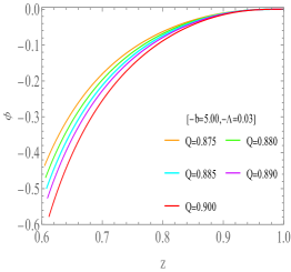
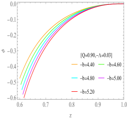
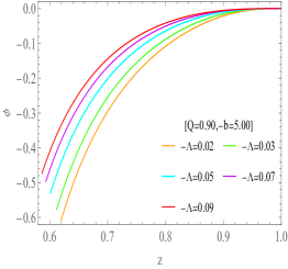
Figure 1: The spatial distribution of the scalar field $\phi$ outside the horizon for various charge $Q$, coupling constant $b$ and cosmological constant $\Lambda$ when the system reaches equilibrium.

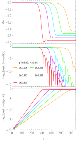
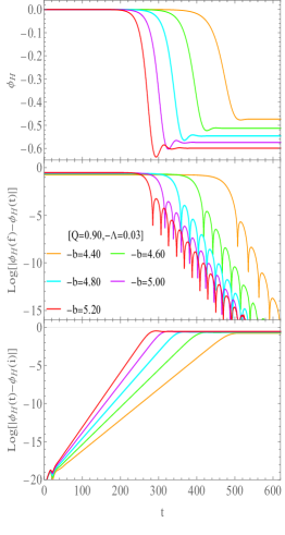
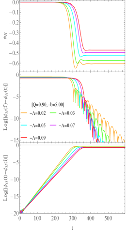
Figure 2: The upper row shows the evolution of the scalar field value $\phi_{H}$ on the horizon. The lower and center rows indicate that $\phi_{H}$ grows exponentially at first and then saturates to an equilibrium value with damped oscillation.

To figure out how the system evolves from the initial bald RN-AdS BH to the final hairy BH, we show the evolution of the scalar field value on the horizon $\phi_{H}$ in the upper row of Fig. 2. One can find that the BH is decorated with scalar hair faster and more heavily for larger $Q$ and stronger coupling $-b$ between the scalar field and Maxwell field. On the contrary, the cosmological constant $\Lambda$ suppresses this phenomenon. These are consistent with the results from Fig. 1.

In the middle and lower rows of Fig. 2, we show the evolution of $\log|\phi_{H}(f)-\phi_{H}(t)|$ and $\log|\phi_{H}(t)-\phi_{H}(i)|$. Here $\phi_{H}(i)=0$ and $\phi_{H}(f)$ are the initial and final scalar field value on the horizon, respectively. The lower row implies that if the RN-AdS BH is in the unstable regime, any initial arbitrarily small perturbation will result in an exponential growth of the scalar field at early times. The middle row implies that the scalar field saturates to an equilibrium value at late times and the final equilibrium BH is endowed with scalar hair. Hence the evolution of the scalar field on the horizon can be approximated by

$$\phi_{H}\approx\begin{cases}\exp(\nu_{i}{t}+\nu_{1}),&\text{early times,}\\ \phi_{H}(f)-\exp(-\nu_{f}{t}+\nu_{2}),&\text{late times.}\end{cases}$$ (26)

Here $\nu_{i}$ is the growth rate of $\phi_{H}$ at early times and $\nu_{f}$ is the imaginary part of dominant mode frequency at late times. $\nu_{1,2}$ are some subdominant terms depending on $Q$, $b$ and $\Lambda$. The lower row of Fig. 2 reveals that $\nu_{i}$ is positively related to $Q$ and $-b$, and negatively related to $-\Lambda$, which means that the time of scalarized BH bifurcating from the initial RN-AdS BH will be shortened during the growth stage for larger $Q$ and $-b$, and prolonged for larger $-\Lambda$. At late times, however, the central row of Fig. 2 shows that during the saturation stage, $\phi_{H}$ takes longer time to converge to its final value for larger $Q,-b$ and smaller $-\Lambda$. On the other hand, the relations between $\nu_{f}$ and $Q,b,\Lambda$ are contrary to those of $\nu_{i}$.

IV.1.2 Misner-Sharp mass of fractional coupling

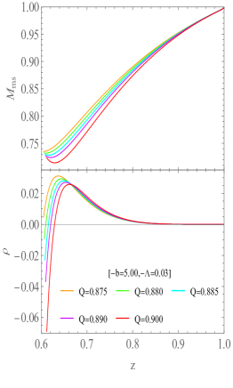
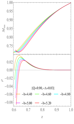
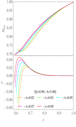
Figure 3: Fractional coupled scalarized BH solutions exhibit negative energy densities $\rho$ in the vicinity of horizon. Note that the left endpoints locate on the BH horizon and we only show the distribution outside the horizon.

The Misner-Sharp mass $M_{ms}$ of scalarized solutions is a function of radius and time. Its final distribution when the system reaches equilibrium is exhibited in the upper row of Fig. 3. It increases to the ADM mass $M=1$ as the radius tends to infinity. However, in the near horizon region, the $M_{ms}$ decreases with radius for large $Q,-b$ and small $-\Lambda$. This implies that there are negative energy distribution near the black hole. In fact, for static solution, the energy density can be expressed as

$$\rho=\frac{\alpha}{2}\left(\frac{\partial{\phi}}{\partial{r}}\right)^{2}+\frac{Q^{2}(1+b\phi^{2})}{2\zeta^{4}},$$ (27)

which follows from $\rho=T_{\mu\nu}Z^{\mu}Z^{\nu}$. Here $T_{\mu\nu}$ is the stress energy tensor in eq. (3), and $Z^{\mu}=(\partial_{t})^{\mu}/\sqrt{\alpha}$. The energy density distribution is shown in the lower row of Fig. 3. One can find that the scalarized BH solution obtained with fractional coupling does have negative energy density in the vicinity of horizon. This is similar to the results found in asymptotically flat spacetime Fernandes:2019 . Actually, the negative energy originates from the second term in eq. (27) since $1+b\phi^{2}<0$ in the vicinity of the horizon. The negative contribution is more significant for stronger coupling and larger charge.

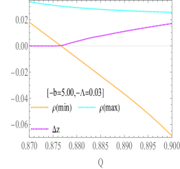
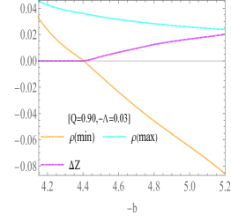
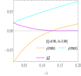
Figure 4: The maximum and minimum of the energy density $\rho$ outside the horizon, the negative energy band $\Delta{z}$ and the minimum of the Misner-Sharp mass versus $Q,b$ and $\Lambda$.

The extremum of $\rho$ and the negative energy band $\Delta{z}$ are shown in Fig. 4. The $\rho(min)$ decreases monotonically with $Q$ or $-b$, while $\Delta{z}$ first remains zero and then increases. This result can also be explained by eq. (27) in which the first term is always positive outside the horizon. For small $Q$ or $-b$, the final scalarized BH has less hair so that the first term is larger than the second term, so the energy density $\rho$ is positive and the negative energy band $\Delta{z}$ is zero. On the one hand, the right row of Fig. 4 shows that the increase of $-\Lambda$ suppresses the negative energy distribution outside the horizon.

IV.1.3 Naked singularity

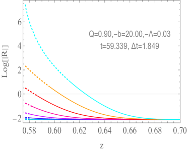
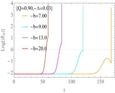
Figure 5: Left: the evolution of scalar curvature $R$ when $Q=0.9,-\Lambda=0.03$ and $-b=20$. The time step between adjacent curves is $\Delta{t}=1.8546$. The upper most curve corresponding to $t=59.3390$, after which our code crashes soon. The dashed parts represent the results in the interior of the apparent horizon. Right: the evolution of scalar curvature on the apparent horizon $R_{H}$ for various $b$ when $Q=0.9,-\Lambda=0.03$ before our code crashes.

The above subsection shows that the negative energy becomes more significant for stronger coupling parameter $-b$. Here we show that $-b$ can not be too large, otherwise a naked singularity will appears inevitably. The left panel of Fig. 5 shows the evolution of the Ricci scalar for $Q=0.9,-\Lambda=0.03$ and $-b=20$. The Ricci scalar explodes in the interior of the apparent horizon. Although our code crashes at late times, we suggest that the curvature singularity moves outwards rapidly and finally passes through the apparent horizon such that a naked singularity forms. From another viewpoint, we show the evolution of the scalar curvature on the apparent horizon $R_{H}$ in the right panel. The $R_{H}$ also explodes with time. For larger $-b$, the $R_{H}$ increases faster and our code crashed earlier. We conclude that for large $-b$, the evolution endpoint of a linearly unstable RN-AdS black hole is a spacetime with naked singularity such that the weak cosmic censorship is violated Wald:1997wa . The cosmic censorship has been tested in EMS theory Corelli:2021ikv , in which they found that naked singularities do not form for certain coupling functions. We will show later that for hyperbolic and power couplings, naked singularities also do not form. In eSTGB theory, the the cosmic censorship has been tested very recently Corelli:2022pio ; Corelli:2022phw . They simulated the mass loss due to evaporation at the classical level using an auxiliary phantom field and suggested that either the weak cosmic censorship is violated or horizonless remnants are produced. Here we find that without introducing phantom field, the cosmic censorship can also be violated.

IV.1.4 Irreducible mass of fractional coupling

Fig. 6 displays the evolution of the BH irreducible mass $M_{ir}$ for various $Q,-b,-\Lambda$. The irreducible mass equals the BH apparent horizon area radius. In the upper row one can find that the irreducible mass never decreases during the evolution, although the weak energy condition is violated, as discussed in the above subsection. This is permissible since the the weak energy condition is a sufficient but not necessary condition for the black hole area increase law HawkingEllis ; Nielsen:2008cr . The nonlinear evolution exhibits no other obvious pathologies apart from the negative energy density. The scalarized solutions are both thermodynamically and dynamically preferred.

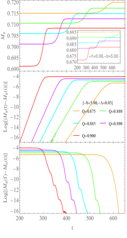
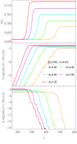
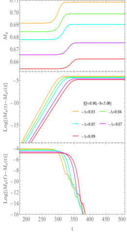
Figure 6: The evolution of irreducible mass $M_{ir}$ for various coupling constant $b$, charge $Q$ and cosmological constants $\Lambda$.

The irreducible mass increases with $Q$ and $-b$. This can be understood from the coupling term between the Maxwell field and the scalar field in the action. For larger $Q$ or $-b$, the coupling is stronger. More energy will be transferred from the Maxwell field to the scalar field. The BH can swallow more scalar field and its area grows. The cosmological constant $\Lambda$, however, puts more stringent condition for the spontaneous scalarisation. Comparing the evolution of $M_{ir}$ at different $\Lambda$ in the upper-left inset of Fig. 6, within certain parameter ranges, the original scalar-free BH is stabilized due to the increase of $-\Lambda$. In fact, in asymptotic AdS spacetime, the tachyonic instability occurs only when its effective mass-squared is less than the Breitenlohner-Freedman bound $\mu^{2}_{BF}=\frac{3\Lambda}{4}$ BFbound ; Zhang:20211 ; Guo:2021 . For large enough $-\Lambda$, the tachyonic instability can be quenched.

Another interesting feature is that the evolution of irreducible mass $M_{ir}$ can be roughly divided into two stages. The center and lower rows of Fig. 6 illustrate that both the early stage and the late stages follow exponential evolution:

$$M_{ir}(t)\approx\begin{cases}M_{ir}(i)+\exp(\gamma_{i}{t}+\gamma_{1}),&\text{early times,}\\ M_{ir}(f)-\exp(-\gamma_{f}{t}+\gamma_{2}),&\text{late times.}\end{cases}$$ (28)

Here $\gamma_{i}$ and $\gamma_{f}$ are the exponential growth rate and saturation rate of $M_{ir}$, respectively. $M_{ir}(i)$ and $M_{ir}(f)$ are the initial and final irreducible mass of the BH, respectively. $\gamma_{1,2}$ are some terms less important. Note that $M_{ir}(i)$ of the initial RN-AdS BH depends on $Q$ and $\Lambda$. From the middle row of Fig. 6, the relationship between $\gamma_{i}$ and $Q,b,\Lambda$ is analogous to those of the $\phi_{H}$ at the horizon. However, the saturation stage is stepped rather than damped oscillation, as shown in the lower row of Fig. 6.

IV.1.5 $\phi_{3}$ of fractional coupling

Now we investigative the evolution of coefficient $\phi_{3}$ of the scalar field at spacial infinity. Fig. 7 shows that the evolution of $\phi_{3}$ resembles the evolution of $\phi_{H}$, which can also be divided roughly into two stages. At early stage, it increases exponentially. At late time, it converges to the equilibrium value $\phi_{3}(f)$ with damped oscillation which resembles the quasinormal mode. Its evolution can be approximated by

$$\phi_{3}\approx\begin{cases}\exp(\eta_{i}{t}+\eta_{1}),&\text{early times,}\\ \phi_{3}(f)-\exp(-\eta_{f}{t}+\eta_{2}),&\text{late times.}\end{cases}$$ (29)

Here $\eta_{i}$ is the grows rate of $\phi_{3}$ at early times, and $\eta_{f}$ the imaginary part of the dominant mode frequency of $\phi_{3}$ at late times. $\eta_{1,2}$ are some terms less important. The lower row of Fig. 7 shows that $\eta_{i}$ is positively related to $Q,-b$ and negatively related to $\Lambda$. Meanwhile $\eta_{f}$ has contrary relations to $Q,-b,\Lambda$.

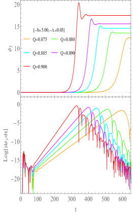
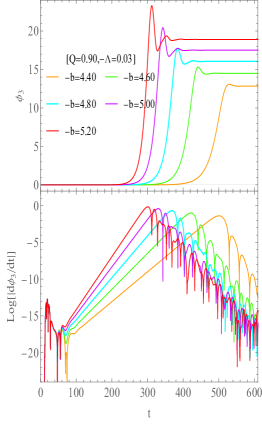
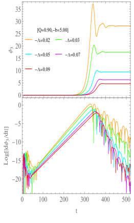
Figure 7: The evolution of $\phi_{3}$. It resembles the evolution of $\phi_{H}$ , although the sign is reversed (upper row). The lower row shows the evolution of $\log|\frac{d\phi_{3}}{dt}|$.

There are universal and robust relationships between $\phi_{H}$, $M_{ir}$ and $\phi_{3}$ during the evolution:

$$\gamma_{i}=2\nu_{i}=2\eta_{i},\gamma_{f}=2\nu_{f}=2\eta_{f}.$$ (30)

This relationship can be understood for an intermediate solution which can be approximated by a static solution. For a static solution, the variables $S$, $\alpha$ and $P$ are zero on the horizon. So combining (9,10,11,13) and (15) one can find $\partial_{t}S$, $\partial_{t}\zeta\propto{\delta\phi^{2}}$ for the intermediate solution. Since $S(r_{H},t)=0$ and (21) states that $M_{ir}=\zeta(r_{H},t)$, we can deduce that $\dot{M}_{ir}=\dot{\zeta}(r_{H},t)=-\frac{\partial_{t}S}{\partial_{r}S}\partial_{r}\zeta+\partial_{t}\zeta|_{r_{H}}\propto{\dot{\phi}_{H}^{2}}$. Since at early and late times, the evolution can be approximated by the perturbations for the initial and final BHs, respectively, this leads to the relations (30). These relations have been found in other cases Zhang:2022 ; Zhang:20211 ; zhang:20221 ; zhang:20222 .

IV.2 Results for Power-Law and Hyperbolic Coupling

In this subsection, we consider the dynamics of the spontaneous scalarization with coupling functions $f_{H}=\cosh{\sqrt{-2b}\phi}$ and $f_{P}=1-b\phi^{2}$. The results are shown in Fig. 8. It can be seen that the evolution of $M_{ir}$ and $\phi_{H},\phi_{3}$ still obeys the exponential growth at early stage and saturates to the equilibrium value at late times. But now the Misner-Sharp mass monotonically increases to the ADM mass at spacial infinity. In other words, there is no negative energy distribution outside the BH horizon. We find that the dynamical features of the spontaneous scalarization for power-law and hyperbolic coupling $f_{E}=\exp(-b\phi^{2})$ in the AdS-EMS gravity model are similar to the case with exponential coupling which has been studied in Zhang:20211 , and we will not repeat the text.

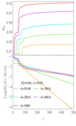
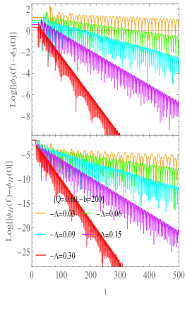
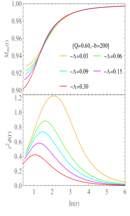
Figure 8: Left column: the evolution of the irreducible mass $M_{ir}$ for models with hyperbolic coupling function. Middle column: the evolution of $\phi_{3}$ and $\phi_{H}$. Right column: the final profiles of the Misner-Sharp mass and $r^{2}\phi$ for different $\Lambda$.

V Conclusion

We have focused attention on the dynamical spontaneous scalarization in the asymptotically AdS spacetime in EMS models. We have discussed three different forms of coupling function, which share the same form of the leading-order expansion $1-b\phi^{2}$ in the limit of small scalar field. Under certain conditions, we have found that the bald RN-AdS BH can be transformed into scalarized BH, which is preferred in thermodynamics. We have explored the effects of the BH charge $Q$, coupling strength parameter $b$ and cosmological constant $\Lambda$ on the dynamical process in the scalarization. When the system reaches equilibrium, the extreme value of $\phi$ always locates at the horizon (denoted as $\phi_{H}$). Starting from the initial bald RN-AdS BH, we find that $\phi_{H}$ grows exponentially at the early stage of the dynamical evolution in the scalarization. At the late stage in the process of scalarization, $\phi_{H}$ converges to an equilibrium value through damped oscillation. We find that the scalarization is enhanced by larger values of $Q,-b$ but suppressed with the increase of $\Lambda$. We hae also investigated the evolution of $\phi_{3}$, and find $\phi_{3}$ evolves similarly to $\phi_{H}$.

The irreducible mass $M_{ir}$ never decreases during the dynamical spontaneous scalarization of the BH. Since $M_{ir}$ is the horizon area radius and the BH entropy is proportional to the horizon area, this feature is a signal that the second law of thermodynamics is obeyed, although the weak energy condition is violated in models with fractional coupling function. $M_{ir}$ grows exponentially at early times and saturates also exponentially to the final value at late times. The corresponding growth coefficient $\gamma_{i}$ and saturation coefficient $\gamma_{f}$ increase with $Q$ and $-b$. The increase of $\gamma_{i,f}$ can shorten the growth and saturation time of $M_{ir}$. On the other hand, the cosmological constant plays a contrary role that prolongs the time for dynamical scalarization.

For EMS model with fractional coupling, there is negative energy distribution near the BH horizon such that the weak energy condition is violated. The negative energy region is stretched with the increase of $Q$ and $-b$ and narrowed with $\Lambda$. However, $Q$ and $-b$ cannot be too large. Once these parameters reach maximum thresholds, a naked singularity will appears and the weak cosmic censorship is violated. Compared with fractional coupling, the cases with hyperbolic coupling $f_{H}(\phi)$ and power-law coupling $f_{P}(\phi)$ in AdS spacetime do not violate energy condition. Note that $f_{H}(\phi)$, $f_{P}(\phi)$ and exponential coupling $f_{E}(\phi)$ share the same leading order expansion in perturbations. Therefore, the dynamic evolution features of $f_{H}(\phi)$ and $f_{P}(\phi)$ can be similar to those with the exponential coupling $f_{E}(\phi)$ Zhang:20211 .

References

- (1) E. Berti et al., “Testing General Relativity with Present and Future Astrophysical Observations,” Class. Quant. Grav., vol. 32, p. 243001, 2015.
- (2) L. Barack et al., “Black holes, gravitational waves and fundamental physics: a roadmap,” 2018.
- (3) B. P. Abbott et al., “Observation of Gravitational Waves from a Binary Black Hole Merger,” Phys. Rev. Lett., vol. 116, no. 6, p. 061102, 2016.
- (4) B. P. Abbott et al., “GW170104: Observation of a 50-Solar-Mass Binary Black Hole Coalescence at Redshift 0.2,” Phys. Rev. Lett., vol. 118, no. 22, p. 221101, 2017.
- (5) B. P. Abbott et al., “GWTC-1: A Gravitational-Wave Transient Catalog of Compact Binary Mergers Observed by LIGO and Virgo during the First and Second Observing Runs,” 2018.
- (6) P. V. P. Cunha and C. A. R. Herdeiro., “Shadows and strong gravitational lensing: a brief review,” Gen. Rel. Grav., vol. 50, no. 4, p. 42, 2018.
- (7) K. Akiyama et al. [Event Horizon Telescope], “First M87 Event Horizon Telescope Results. I. The Shadow of the Supermassive Black Hole,” Astrophys. J., vol. 875, no. 1, L1, 2019.
- (8) K. Akiyama et al. [Event Horizon Telescope], “First M87 Event Horizon Telescope Results. IV. Imaging the Central Supermassive Black Hole,” Astrophys. J. Lett., vol. 875, no. 1, L4, 2019.
- (9) K. Akiyama et al. [Event Horizon Telescope], “First M87 Event Horizon Telescope Results. VI. The Shadow and Mass of the Central Black Hole,” Astrophys. J. Lett., vol. 875, no. 1, L6, 2019.
- (10) Werner Israel., “Event horizons in static vacuum space-times,” Phys. Rev., vol. 164, no. 10, p. 1776, 1967.
- (11) B. Carter., “Axisymmetric Black Hole Has Only Two Degrees of Freedom,” Phys, Rev. Lett., vol. 26, no. 10, p. 331, 1971.
- (12) P. T. Chrusciel, J. Lopes Costa, and M. Heusler, “Stationary Black Holes: Uniqueness and Beyond,” Living Rev. Rel., vol. 15, p. 7, 2012.
- (13) M. S. Volkov and D. V. Galtsov., “Non-Abelian Einstein Yang-Mills black holes,” JETP Lett., vol. 50, no. 7, p. 346, 1989.
- (14) P. Bizon., “Colored black holes,” Phys. Rev. Lett., vol. 64, no. 24, p. 2884, 1990.
- (15) B. R. Greene, S. D. Mathur, and C. M. O’Neill., ”Eluding the no hair conjecture: Black holes in spontaneously broken gauge theories,” Phys. Rev., vol. D 47, no. 6, p. 2242, 1993.
- (16) K. I. Maeda, T. Tachizawa, T. Torii, and T. Maki., “Stability of nonAbelian black holes and catastrophe theory,” Phy. Rev. Lett., vol. 72, no. 4, p. 450, 1994.
- (17) H. Luckock and I. Moss., “Black holes have skyrmion hair,” Phys. Lett., vol. B 176, no. 3-4, p. 341, 1986.
- (18) S. Droz, M. Heusler and N. Straumanm., “New black hole solutions with hair,” Phys. Lett., vol. B 268, no. 3-4, p. 371, 1991.
- (19) J. D. Bekenstein., “Exact solutions of Einstein conformal scalar equations,” Annals Phys., vol. 82, no. 2, p. 535, 1974.
- (20) P. Kanti, N. E. Mavromatos, J. Rizos, K. Tamvakis, and E. Winstanley., “Dilatonic black holes in higher curvature string gravity,” Phys. Rev., vol. D 54, no. 8, p. 5049, 1996.
- (21) C. Y. Zhang, P. Liu, Y. Liu, C. Niu, and B. Wang., “Evolution of Anti-de Sitter black holes in Einstein-Maxwell-dilaton theory,” Phys. Rev., vol. D 105, no. 2, p. 024010, 2022.
- (22) C. Y. Zhang, P. Liu, Y. Liu, C. Niu, and B. Wang., “Dynamical scalarization in Einstein-Maxwell-dillton theory,” Phys. Rev., vol. D 105, no. 2, p. 024073, 2022.
- (23) T. Damour and G. Esposito-Farese., “Nonperturbative strong field effects in tensor-scalar theories of gravitation,” Phys. Rev. Lett., vol. 70, no. 15, p. 2220, 1993.
- (24) T. Damour and G. Esposito-Farese., “Tensor-scalar gravity and binary pulsar experiments,” Phys. Rev., vol. D 54, no. 2, p. 1474, 1996.
- (25) T. Harada, “Stability analysis of spherically symmetric star in scalar-tensor theories of gravity,” Prog. Theor. Phys., vol. 98, no. 2, p. 359, 1997.
- (26) V. Cardoso, I. P. Carucci, P. Pani, and T. P. Sotiriou., “Black holes with surrounding matter in scalar-tensor theories,” Phys. Rev. Lett., vol. 111, no. 11, p. 111101, 2013.
- (27) V. Cardoso, I. P. Carucci, P. Pani, and T. P. Sotiriou., “Matter around Kerr black holes in scalar-tensor theories: scalarization and superradiant instability,” Phys. Rev., vol. D 88, no. 4, p. o44056, 2013.
- (28) C. Y. Zhang, S. J. Zhang, and B. Wang., “Superradiant instability of Kerr-de Sitter black holes in scalar-tensor theory,” JHEP 1408, 011(2014).
- (29) G. Antoniou, A. Bakopoulos, and P. kanti., “Evasion of No-Hair Theorems and Novel Black-Hole Solutions in Gauss-Bonnet Theories,” Phys. Rev. Lett., vol. 120, no. 13, p. 131102, 2018.
- (30) D. D. Doneva and S. S. Yazadjiev., “New Gauss-Bonnet Black Holes with Curvature-Induced Scalarization in Extended Scalar-Tensor Theories,” Phys. Rev. Lett., vol. 120, no. 13, p. 131103, 2018.
- (31) H. O. Silva, J. Sakstein, L. Gualtieri, T. S. Sotiriou, and Emanuele., “Spontaneous scalarization of black holes and compact stars from a Gauss-Bonnet coupling,” Phys. Rev. Lett., vol. 120, no. 13, p. 131104, 2018.
- (32) J. L. Blázquez-Salcedo, D. D. Doneva, J. Kunz and S. S. Yazadjiev., ”Radial perturbations of the scalarized Einstein-Gauss-Bonnet black holes,” Phys. Rev., vol. D 98, no. 8, p. 084011, 2018.
- (33) C. A. R. Herdeiro and E. Radu., “Black hole scalarisation from the breakdown of scale invariance,” Phys. Rev., vol. D 99, no. 8, p. 084039, 2019.
- (34) Y. Brihaye, C. Herdeiro, and E. Radu., “The scalarized Schwarzschild-NUT spacetime,” Phys. Lett., vol. B 788, p. 295, 2019.
- (35) C. A. R. Herdeiro, E. Radu, N. Sanchis-Gual, and J. A. Font., “Spontaneous Scalarization of Charged Black Holes,” Phys. Rev. Lett., vol. 121, no. 10, p. 101102, 2018.
- (36) G. Antoniou, A. Bakopoulos, and P. Kanti., “Black-hole solutions with scalar hair in Einstein-scalar-Gauss-Bonnet theories,” Phys. Rev., vol. D 97, no. 8, p. 084037, 2018.
- (37) Y. S. Myung and D. C. Zou., “Gregory-Laflamme instability of black hole in Einstein-scalar-Gauss-Bonnet theories,” Phys. Rev., vol. D 98, no. 2, p. 024030, 2018.
- (38) M. Minamitsuji and T. Ikeda., ”scalarized black holes in the presence of the coupling to Gauss-Bonnet gravity,” Phys. Rev., vol. D 99, no. 4, p. 044017, 2019.
- (39) P. V. P. Cunha, C. A. R. Herdeiro, and E. Radu., “Spontaneously Scalarized Kerr Black Holes in Extended-Scalar-Tensor-Gauss-Bonnet Gravity,” Phys. Rev. Lett., vol. 1223, no. 1, p. 011101,2019.
- (40) C. F. B. Macedo, J. Sakstein, E. Berti, L. Gualtieri, H. O. Silva, and T. P. Sotiriou, “Self-interactions and Spontaneous Black Hole Scalarization,” Phys. Rev., vol. D 99, no. 10, p. 104041, 2019. [arXiv:1903.06784 [gr-qc]].
- (41) C. A. R. Herdeiro, E. Radu, H. O. Silva, T. P. Sotiriou, and N. Yunes, “Spin-induced scalarized black holes,” Phys. Rev. Lett., vol. 126, no. 1, p. 011103, 2021. [arXiv:2009.03904 [gr-qc]].
- (42) E. Berti, L. G. Collodel, B. Kleihaus, and J. Kunz, “Spin-induced black-hole scalarization in Einstein-scalar-Gauss-Bonnet theory,” Phys. Rev. Lett., vol. 126, no. 1, p. 011104, 2021. [arXiv:2009.03905 [gr-qc]].
- (43) A. Dima, E. Barausse, N. Franchini, and T. P. Sotiriou, “Spin-induced black hole spontaneous scalarization,” Phys. Rev. Lett., vol. 125, no.23, p. 231101, 2020. [arXiv:2006.03095 [gr-qc]].
- (44) A. Bakopoulos, G. Antoniou, and P. Kanti, “Novel Black-Hole Solutions in Einstein-Scalar-Gauss-Bonnet Theories with a Cosmological Constant,” Phys. Rev., vol. D 99, no. 6, p. 064003, 2019. [arXiv:1812.06941 [hep-th]].
- (45) J. L. Ripley and F. Pretorius, “Hyperbolicity in Spherical Gravitational Collapse in a Horndeski Theory,” Phys. Rev., vol. D 99, no. 8, p. 084014, 2019. [arXiv:1902.01468 [gr-qc]].
- (46) J. L. Ripley and F. Pretorius, “Dynamics of a Z2 symmetric EdGB gravity in spherical symmetry,” Class. Quant. Grav., vol. 37, no. 15, p. 155003, 2020. [arXiv:2005.05417 [gr-qc]].
- (47) W. E. East and J. L. Ripley, “Evolution of Einstein-scalar-Gauss-Bonnet gravity using a modified harmonic formulation,” Phys. Rev., vol. D 103, no.4, p. 044040, 2021. [arXiv:2011.03547 [gr-qc]].
- (48) W. E. East and J. L. Ripley, “Dynamics of Spontaneous Black Hole Scalarization and Mergers in Einstein-Scalar-Gauss-Bonnet Gravity,” Phys. Rev. Lett., vol. 127, no.10, p. 101102, 2021. [arXiv:2105.08571 [gr-qc]].
- (49) D. D. Doneva and S. S. Yazadjiev, “Dynamics of the nonrotating and rotating black hole scalarization,” Phys. Rev., vol. D 103, no. 6, p. 064024, 2021. [arXiv:2101.03514 [gr-qc]].
- (50) H. J. Kuan, D. D. Doneva, and S. S. Yazadjiev, “Dynamical Formation of Scalarized Black Holes and Neutron Stars through Stellar Core Collapse,” Phys. Rev. Lett., vol. 127, no.16, p. 161103, 2021. [arXiv:2103.11999 [gr-qc]].
- (51) D. D. Doneva and S. S. Yazadjiev, “Beyond the spontaneous scalarization: New fully nonlinear mechanism for the formation of scalarized black holes and its dynamical development,” Phys. Rev., vol. D 105, no.4, p. L041502, 2022. [arXiv:2107.01738 [gr-qc]].
- (52) H. O. Silva, H. Witek, M. Elley, and N. Yunes, “Dynamical Descalarization in Binary Black Hole Mergers,” Phys. Rev. Lett., vol. 127, no.3, p. 031101, 2021. [arXiv:2012.10436 [gr-qc]].
- (53) D. D. Doneva, A. Vañó-Viñuales, and S. S. Yazadjiev, “Dynamical descalarization with a jump during black hole merger,” [arXiv:2204.05333 [gr-qc]].
- (54) P. G. S. Fernandes, C. A. R. Herdeiro, A. M. Pombo E. Radu, and N. Sanchis-Gual., “Spontaneous Scalarisation of Charged Black Holes: coupling Dependence and Dynamical Features,” Class. Quant. Grav., vol. 36, no. 13, p. 134002, 2019.
- (55) J. L. Blázquez-Salcedo, C. A. Herdeiro, J. Kunz, A. M. Pombo, and E. Radu., “Einstein-Maxwell-scalar black holes: the hot, the cold and the bald,” Phys. Lett., vol. B 806, p. 135439, 2020.
- (56) Y. S. Myung and D. C. Zou., “Instability of Reissner-Nordstr’́om black hole in Einsten-Maxwell-scalar theory,” Eur. Phys. J, vol. 79, no. 3, p. 273, 2019.
- (57) D. Astefanesei, C. Herdeiro, and A. Pombo., “Einstein-Maxwell-scalar black holes: classes of solutions, dyons and extremality,” JHEP, vol. 10, p. 078, 2019.
- (58) Y. Brihave, C. Herdeiro, and E. Radu., “Black Hole Spontaneous Scalarisation with a Positive Cosmological Constant,” Phys. Lett. B., vol. 802, p. 135269, 2020.
- (59) P. G. S. Fernandes, C. A. R. Herdeiro, A. M. Pombo, E. Radu, and N. Sanchis-gual., “Charged black holes with axionic-type couplings: Classes of solutions and dynamical scalarization,” Phys. Rev. D, vol. 100, no. 4, p. o44004, 2019.
- (60) W. Xiong, P. Liu, C. Niu, C. Y. Zhang, and B. Wang, “Dynamical spontaneous scalarization in Einstein-Maxwell-scalar theory,” [arXiv:2205.07538 [gr-qc]].
- (61) G. Guo, P. Wang, and H. Wu., “Scalarized Einstein-Maxwell-scalar black holes in anti-de Sitter spacetime,” Eur. Phys. J. C., vol. 81, no. 10, p. 864, 2021.
- (62) C. Y. Zhang, P. Liu, Y. Liu, C. Niu, and B. Wang., “Dynamical charged black hole spontaneous scalarisation in anti-de Sitter spacetimes,” Phys. Rev. D, vol. 104, no. 8, p. 084089, 2021.
- (63) C. Y. Zhang, Q. Chen, Y. Liu, W. K. Luo, Y. Tian, and B. Wang., “Dynamical transitions in scalarization and descalarization through black hole accretion,” [arXiv:2204.09260 [gr-qc]].
- (64) P. M. Chesler and L. G. Yaffe., “Horizon Formation and Far-From-Equilibrium Isotropization in Supersymmetric Yang-Mills Plasma,” Phys. Rev. Lett., vol. 102, no. 21, p. 211601, 2009.
- (65) M. J. Bhaseen, J. P. Gauntlett, B. D. Simons, J. Sonner, and T. Wiseman, “Holographic Superfluids and the Dynamics of Symmetry Breaking,” Phys. Rev. Lett., vol. 110, p. 015301, 2013.
- (66) P. M. Chesler and L. G. Yaffe, ”Numerical solution of gravitational dynamics in asymptotically anti-de Sitter spacetimes,” JHEP 07, 086 (2014) [arXiv:1309.1439 [hep-th]].
- (67) R. A. Janik, J. Jankowski, and H. Soltanpanahi, “Real-Time Dynamics and Phase Separation in a Holographic First Order Phase Transition,” Phys. Rev. Lett., vol. 119, no. 26, p. 261601, 2017
- (68) P. M. Chesler and D. A. Lowe, “Nonlinear Evolution of the AdS4 Superradiant Instability,” Phys. Rev. Lett., vol. 122, no. 18, p. 181101, 2019.
- (69) P. Bosch, S. R. Green, and L. Lehner, “Nonlinear Evolution and Final Fate of Charged Anti-de Sitter Black Hole Superradiant Instability,” Phys. Rev. Lett., vol. 116, no. 14, p. 141102, 2016.
- (70) P. Bosch, S. R. Green, L. Lehner, and H. Roussille, “Excited hairy black holes: Dynamical construction and level transitions,” Phys. Rev.,vol. D 102, no. 4, p. 044014, 2020.
- (71) R. M. Wald, “Gravitational collapse and cosmic censorship,” [arXiv:gr-qc/9710068 [gr-qc]].
- (72) F. Corelli, T. Ikeda and P. Pani, “Challenging cosmic censorship in Einstein-Maxwell-scalar theory with numerically simulated gedanken experiments,” Phys. Rev. D 104, no.8, 084069 (2021) [arXiv:2108.08328 [gr-qc]].
- (73) F. Corelli, M. De Amicis, T. Ikeda and P. Pani, “What is the fate of Hawking evaporation in gravity theories with higher curvature terms?,” [arXiv:2205.13006 [gr-qc]].
- (74) F. Corelli, M. De Amicis, T. Ikeda and P. Pani, “Nonperturbative gedanken experiments in Einstein-dilaton-Gauss-Bonnet gravity: nonlinear transitions and tests of the cosmic censorship beyond General Relativity,” [arXiv:2205.13007 [gr-qc]].
- (75) S. W. Hawking and G. F. R. Ellis, “The large scale structure of space-time,” Cambridge University Press 1973.
- (76) A. B. Nielsen, “Black holes and black hole thermodynamics without event horizons,” Gen. Rel. Grav. 41, 1539-1584 (2009) [arXiv:0809.3850 [hep-th]].
- (77) P. Breitenlohner and D. Z. Freedman., “Stability in gauged extended supergravity,” Ann. Phys. (N.Y.), vol. 144, no. 4, p. 249, 1982.
- (78) C. Y. Zhang, Q. Chen, Y. Liu, W. K. Luo, Y. Tian, and B. Wang., “Critical phenomena in dynamical scalarization of charged black hole,” Phys. Rev. Lett., vol. 128, no. 16, p. 161105, 2022.