Meromorphic functions with a polar asymptotic value

Abstract.

This paper is part of a general program in complex dynamics to understand parameter spaces of transcendental maps with finitely many singular values.

The simplest families of such functions have two asymptotic values and no critical values. These families, up to affine conjugation, depend on two complex parameters. Understanding their parameter spaces is key to understanding families with more asymptotic values, just as understanding quadratic polynomials was for rational maps more generally.

The first such families studied were the one-dimensional slices of the exponential family, $\exp(z)+a$, and the tangent family $\lambda\tan z$. The exponential case exhibited phenomena not seen for rational maps: Cantor bouquets in both the dynamic and parameter spaces, and no bounded hyperbolic components. The tangent case, with its two finite asymptotic values $\pm\lambda i$, is closer to the rational case, a kind of infinite degree version of the latter.

In this paper, we consider a general family that interpolates between $\exp(z)+a$ and $\lambda\tan z$. Our new family has two asymptotic values and a one-dimensional slice for which one of the asymptotic values is constrained to be pole, the “polar asymptotic value” of the title. We show how the dynamic and parameter planes for this slice exhibit behavior that is a surprisingly delicate interplay between that of the $\exp(z)+a$ and $\lambda\tan z$ families.

1. Introduction

A general principle in complex dynamics is that a function’s singular values, the points over which it is not a local homeomorphism,“control” the eventually periodic stable dynamics. Since rational maps have only finitely many singular values, and all stable behavior is eventually periodic, (see [Sul]), a given family exhibits only finitely many different stable dynamical phenomena. The same is true for families of transcendental functions with finitely many singular values, (see [BKL4]), but in this case some of these values must be asymptotic, in the sense that, if $f$ is the map, there is a path $\gamma(t)$ such that $\lim_{t\to 1}\gamma(t)=\infty$, then $\lim_{t\to 1}f(\gamma(t))=v$. Where transcendental functions and rational functions part company more seriously is due to transcendentals having infinite degree, and having a point, infinity, that is an essential singularity and not in the domain. This paper is part of a program to understand both the dynamical properties of functions in such families and the structure of their parameter spaces.

The artistry here is in describing families that are natural and have something interesting to say. The obvious starting point (see for example, [D1, DG, S] was the exponential family $E_{a}(z)=\exp(z)+a$. Here infinity not only has no forward image, it also has no preimages. It is, however, an asymptotic value of $E_{a}$. The only other singular value is the asymptotic value $a$ and as $a$ varies, so do the dynamics. For example, the unstable set contains “Cantor bouquets” of curves, which are families of curves whose cross-section is a Cantor set; and in addition, all components of the parameter plane in which the functions have topologically conjugate dynamics are unbounded.

One natural family, then, generalizes $E_{a}(z)$ to transcendental meromorphic functions with no critical values and exactly two asymptotic or omitted values. In addition to the exponential, this family contains the tangent family, $\lambda\tan z$; its asymptotic values are $\pm\lambda i$ and their orbits are symmetric. Thus, the dynamics are “controlled” by the behavior of either of the asymptotic values. There are parameter values for which the asymptotic values of the functions are prepoles, and these play a special role in the structure of the parameter plane. See [ABF, FK, KK].

Another variation on this theme is to consider the family of functions with two finite asymptotic values and one attracting fixed point. Fixing the derivative at the attracting fixed point determines a one dimensional parameter space. There are tangent maps contained in this family and the local dynamical structure is similar to what we see for $\lambda\tan z$. Because the asymptotic values are not symmetric, however, the parameter plane has properties similar to both the tangent family and rational maps of degree $2$ with an attracting fixed point. See [CJK2, CJK3].

In this paper, we are going to look at a family ${\mathcal{FP}}_{2}$ of functions with two asymptotic values, one of which is fixed and is a pole — the “polar asymptotic value”. The family ${\mathcal{FP}}_{2}$ can be thought of as a hybrid of the tangent and exponential families: in both the dynamical and parameter planes, we have behavior that reflects properties from each of these two families. The significance of having a polar asymptotic value stems from the general fact that an attracting periodic cycle must attract an asymptotic value, but it cannot attract the pole, so the only other asymptotic value must be attracted to it. This implies there can be only one attractive cycle, and its basin of attraction is the full stable set.

On the one hand, this behavior is similar to the exponential family, where one asymptotic value is infinity (a pole of order 0). On the other hand, because here there are prepoles, the non-zero asymptotic value can be a prepole, so we also see similarities with the tangent family. It is this interplay that raises new problems and makes this family of particular interest.

Our analysis of ${\mathcal{FP}}_{2}$ extends ideas introduced in a rather different context, [FK], which studies families with any finite number of singular values, none of which is infinity. For these families we did the analogous procedure for getting a one-dimensional slice: fix the behavior of all but one of the singular values so that each is attracted to a cycle, and let the last one, an asymptotic value, remain free. There are components of this slice in which the functions have topologically conjugate dynamics. In these families, the functions are hyperbolic, meaning that the orbits of the singular values are disjoint from the unstable set, the orbit of the from the Julia set. Hyperbolicity allows these components to be fully characterized, and in particular, it was shown that they have a unique special boundary point that can be characterized in two ways: first, the free asymptotic value is a prepole and second, as this boundary point is approached from within the component, the derivative along the attracting cycle tends to zero. We called points with these properties virtual cycle parameters and virtual centers, respectively.

To return to our family ${\mathcal{FP}}_{2}$: The polar asymptotic value always belongs to the unstable set, so the functions in ${\mathcal{FP}}_{2}$ can not be hyperbolic. Nevertheless, the parameter space contains components in which the dynamics are topologically conjugate. We will describe how these “pseudo-hyperbolic components” are situated as a function of the free asymptotic value. There are values of the parameter for which the free asymptotic value is a prepole, and here we use ideas from [FK] and from . These values are virtual cycle parameters, and they again play a role as virtual centers, in this case, for the pseudo-hyperbolic components.

Before getting to the general theorems, let us look at the somewhat special case where the attractive cycle is a fixed point, whose dynamical picture is very much like that of $E_{a}(z)$, where $a$ is attracted to a fixed point. By analogy to that case we prove:

Theorem (Theorem A).

The Julia set contains Cantor bouquets at infinity as well as at each of the poles and prepoles and if $f$ has an attracting fixed point, the stable set is a completely invariant connected set and the Cantor bouquets comprise its full complement.

Going back to the early work on quadratic maps (see e.g. [DH]), a standard approach to studying both the dynamic and parameter spaces is to find a combinatorial scheme to encode the dynamics. The idea is to label the inverse branches of a function with integers by assigning an integer $k$ to each pole and to the inverse branch $F_{k}$ that maps infinity to that pole. For definiteness, we assume that $0$ is the polar asymptotic value and $F_{0}(\infty)=0$. In this way, we assign to each prepole a sequence of integers called its kneading sequence. In particular, if a parameter is a virtual cycle parameter, it has a kneading sequence.

We also define a kneading sequence for each attractive cycle by going backwards around the cycle and reading from right to left. This is again consistent with past experience. Now, however, the polar asymptotic value makes the situation much more interesting, because of the inverse branch that takes infinity to the polar asymptotic value. Points in the attractive cycle can bounce back and forth from a neighborhood of infinity to a neighborhood of the polar asymptotic value. If that doesn’t happen, we call the cycle regular. If part of the cycle bounces, we call the cycle hybrid, and if the whole cycle bounces, we call it unipolar.

We can completely characterize the types of kneading sequences that can occur:

Theorem (Theorem B).

Let $f$ be a pseudo-hyperbolic map whose attracting cycle $\{z_{0},\ldots,z_{n-1}\}$ has period $n$. Let $F_{k_{i}}$ denote the branch of $f^{-1}$ such that $F_{k_{i}}(z_{i})=z_{i-1}$, $i=n-1,\ldots 2$. For reasons that will be clear later, we use the symbol $*$ for the branch that takes $z_{1}$ to $z_{0}$. We write the kneading sequence as $*k_{1}\cdots k_{n-1}$.

The kneading sequence for $f$ is one of:

1. Regular sequence: $*k_{1}\cdots k_{n-1}$ where $k_{n-1}\neq 0$ or

2. Unipolar sequence: $*k_{1}0\cdots k_{n-2}0$, the period is odd so the sequence contains an even number of digits after the $*$; all the even ones but not all the odd ones are zero,

3. Hybrid sequence: $*k_{1}\cdots k_{l}k_{l+1}0\cdots k_{n-2}0$, $l>1$, $k_{l},k_{l+1}\neq 0$.

Functions in the same pseudo-hyperbolic component have the same kneading sequences, so the kneading sequences can be used to label these components. Because these functions have no critical values, the derivative at any point in the cycle can never be zero. A boundary point at which this derivative does have limit $0$ is again called a virtual center. Using techniques similar to those in [FK] we prove

Theorem (Theorem C).

Every pseudo-hyperbolic component has a unique virtual center and this boundary point is a virtual cycle parameter.

The main result is essentially a converse to this theorem.

Theorem (Theorem D).

1. Given any unipolar kneading sequence, there is a pseudo-hyperbolic component with this kneading sequence. It is unbounded in the half plane, and as the parameter tends to $\infty$ in the component, the multiplier tends to zero.

2. Given any regular kneading sequence, there is a component with this sequence and its virtual center is the virtual cycle parameter corresponding to the sequence.

3. Given any hybrid kneading sequence, there is a component with this sequence; its virtual center is the virtual cycle parameter corresponding to the first $l$ terms of the sequence .

The paper is organized as follows:

We start by briefly reviewing the basic theory. The family ${\mathcal{FP}}_{2}$ and its virtual cycles are defined, and then the rest of the first half of the paper is devoted to proving Theorems A and B. A key first step to understanding the dynamics is to examine the effect of the polar asymptotic value on the structure of the pre-asymptotic tracts of both asymptotic values. This leads to a proof of theorem A. We can then define kneading sequences for ${\mathcal{FP}}_{2}$, which leads into the proof of theorem B.

In the second half of the paper, we turn to the parameter space and prove theorems C and D. We conclude with some results about parameters in the complement of the pseudo-hyperbolic components and describe some interesting open questions.

This paper is dedicated to Dennis Sullivan who brought the second author into this field in the his early years as Einstein Professor. He showed how her work in Teichmüller theory could be the foundation for looking at the newly developing theory of complex dynamics. This helped her see a new direction for her research and led to some of the work of which she is proudest.

2. Dynamics

Here we review the basic definitions, concepts and notations we will use. We refer the reader to standard sources on meromorphic dynamics for details and proofs. See e.g. [B, BF, BKL1, BKL2, BKL3, BKL4, DK, KK].

We denote the complex plane by ${\mathbb{C}}$, the Riemann sphere by $\widehat{\mathbb{C}}$ and the unit disk by ${\mathbb{D}}$. We denote the punctured plane by ${\mathbb{C}}^{*}={\mathbb{C}}\setminus\{0\}$ and the punctured disk by ${\mathbb{D}}^{*}={\mathbb{D}}\setminus\{0\}$.

Given a family of meromorphic functions, $\{f_{\lambda}(z)\}$, we look at the orbits of points formed by iterating the function $f(z)=f_{\lambda}(z)$. If $f^{k}(z)=\infty$ for some $k>0$, $z$ is called a prepole of order $k$ — a pole is a prepole of order $1$. For meromorphic functions, the poles and prepoles have finite orbits that end at infinity. The Fatou set or stable set, $F_{f}$, consists of those points at which the iterates form a normal family. The Julia set $J_{f}$ is the complement of the Fatou set and contains all the poles and prepoles.

A point $z$ such that $f^{n}(z)=z$ is called periodic. The minimal such $n>0$ is called the period. Periodic points are classified by their multipliers, $m(z)=(f^{n})^{\prime}(z)$ where $n$ is the period: they are repelling if $|m(z)|>1$, attracting if $0<|m(z)|<1$, super-attracting if $m=0$ and neutral otherwise. A neutral periodic point is parabolic if $m(z)=e^{2\pi ip/q}$ for some rational $p/q$. The Julia set is the closure of the repelling periodic points. For meromorphic $f$, it is also the closure of the prepoles, (see e.g. [BKL1]).

If $D$ is a component of the Fatou set, either $f^{n}(D)\subseteq f^{m}(D)$ for some integers $n,m$ or $f^{n}(D)\cap f^{m}(D)=\emptyset$ for all pairs of integers $m\neq n$. In the first case $D$ is called eventually periodic and in the latter case it is called wandering. The periodic cycles of stable domains are classified as follows:

• Attracting or super attracting if the periodic cycle of domains contains an attracting or superattracting cycle in its interior.

• Parabolic if there is a parabolic periodic cycle on its boundary.

• Rotation if $f^{n}:D\rightarrow D$ is holomorphically conjugate to a rotation map. Rotation domains are either simply connected or topological annuli. These are called Siegel disks and Herman rings respectively.

• Essentially parabolic, or Baker, if there is a point $z_{\infty}\in\partial D$ such that for every $z\in D$, $\lim_{k\to\infty}f^{nk}(z)=z_{\infty}$ and $f$ is not defined at the point $z_{\infty}$.

A point $v$ is a singular value of $f$ if $f$ is not a regular covering map over $v$.

• $v$ is a critical value if for some $z$, $f^{\prime}(z)=0$ and $f(z)=v$.

• $v$ is an asymptotic value for $f$ if there is a path $\gamma(t)$ such that $\lim_{t\to\infty}\gamma(t)=\infty$ and $\lim_{t\to\infty}f(\gamma(t))=v$.

• $v$ is a logarithmic asymptotic value if $U$ is a neighborhood of $v$ and there is some component $V$ of $f^{-1}(U\setminus\{v\})$, called an asymptotic tract of $v$, on which $f$ is a universal covering.. Isolated asymptotic values are always logarithmic.

• The set of singular values $S_{f}$ consists of the closure of the critical values and the asymptotic values. The post-singular set is

  $$P_{f}=\overline{\cup_{v\in S_{f}}\cup_{n=0}^{\infty}f^{n}(v)}.$$

  For notational simplicity, if a prepole $p$ of order $n$ is a singular value, $\cup_{n=0}^{n}f^{n}(p)$ is a finite set with $f^{n}(p)=\infty$.

A standard result in dynamics is that each attracting, superattracting, parabolic or Baker cycle of domains contains a singular value. Moreover, unless the cycle is superattracting, the orbit of the singular value is infinite and accumulates on the cycle, or the fixed point of the Baker domain. The boundary of each rotation domain is contained in the accumulation set of the forward orbit of a singular value. (See e.g. [M], chap 8-11 or [B], Sect.4.3.)

The meromorphic functions in the family ${\mathcal{FP}}_{2}$, which are the focus of this paper, have no critical values and exactly two finite simple asymptotic values, one of which is always pole. Since the derivative of such a function is never zero, no function in ${\mathcal{FP}}_{2}$ can have a superattracting cycle.

It follows from [DK, BKL4] that functions in ${\mathcal{FP}}_{2}$ never have wandering domains and from [DK] that they do not have Baker domains. The arguments in [CK2] that prove that there are no Herman rings for the family $\lambda\tan^{p}z^{q}$ also show the same is true for the family ${\mathcal{FP}}_{2}$.

3. The family ${\mathcal{FP}}_{2}$

Functions with exactly two asymptotic values and no critical values are Möbius transformations of the exponential function $e^{kz}$ for arbitrary $k\in\mathbb{C}^{*}$. Because the dynamics are invariant under conjugation by a conformal isomorphism, we may fix the essential singularity at infinity and set $k=2$. We will restrict to those functions for which one asymptotic value is a pole, and we may take that pole to be $0$. If the other asymptotic value is denoted by $\lambda\in{\mathbb{C}}^{*}$, the function can be written as

$$f_{\lambda}(z)=f(z)=\frac{\lambda}{1-e^{-2z}}.$$

Set ${\mathcal{FP}}_{2}=\{f_{\lambda}(z),\lambda\in{\mathbb{C}}^{*}\}$. Since the asymptotic value $0$ is a pole, the dynamics of $f_{\lambda}$ are determined only by the orbit of $\lambda$. We call this the family of unipolar maps.

Note that

$$f_{\lambda}:\mathbb{C}\to\widehat{\mathbb{C}}\setminus\{0,\lambda\}$$

is a universal covering and therefore there are infinitely many inverse branches $F_{k}$ which we can define by setting $F_{k}(\infty)=k\pi i$, $k\in\mathbb{Z}$.

Definition 1.

Let $p$ be a prepole of $f_{\lambda}$ of order $n$, that is, $f^{n}_{\lambda}(p)=\infty$ for some smallest integer $n$. If $F_{k_{1}}\circ\cdots\circ F_{k_{n}}(\infty)=p$, we define the address of $p$ as $k_{1}\cdots k_{n}$.

For example, the address of the pole $k\pi i$ is $k$.

3.1. Virtual cycles

Previous work, [ABF, FK, KK, CK1, CK2, CJK1, CJK2, CJK3], contains the following definition.

Definition 2.

Suppose $f$ is in a holomorphic family of meromorphic functions whose dynamics depend on the parameter $\lambda$ and that $v(\lambda)$ is an asymptotic value for $f$. If, for some value $\lambda^{*}$, and some integer $n$, $f^{n}(v(\lambda^{*}))=\infty$, then the orbit $\{v(\lambda^{*}),f(v(\lambda^{*})),\ldots,f^{n-1}(v(\lambda^{*})),\infty\}$ is called a virtual cycle for $f$ of period $n+1$.

The cycle is virtual in the sense that there exists an asymptotic path $\gamma(t)$ for $v(\lambda^{*})$, such that $\lim_{t\to 1}f(\gamma(t))=\lim_{t\to 1}f^{n+2}(\gamma(t))=v(\lambda^{*})$; that is both $\gamma(t)$ and $f^{n+1}(\gamma(t))$ are asymptotic paths for $v(\lambda^{*})$.

3.1.1. Virtual cycles in $\mathcal{FP}_{2}$

In the works cited above, virtual cycles are of interest because they occur for functions in a family where periodic cycles have “disappeared”. The functions in the family $\mathcal{FP}_{2}$ have two asymptotic values $0$ and $\lambda$. Since $0$ is a pole for all the functions in our family, it belongs to a virtual cycle for ALL our functions and so these virtual cycles are not like those already studied. We will see that those functions for which $\lambda$ is also a prepole are like those in the cited works.

Definition 3.

Let $\gamma_{1}(t)$ be an asymptotic path for the asymptotic value $0$ of $f_{\lambda}$ such that

$$\lim_{t\to 1^{-}}\gamma_{1}(t)=-\infty,\,\lim_{t\to 1^{-}}f_{\lambda}(\gamma_{1}(t))=0\,\mbox{ and }\lim_{t\to 1^{-}}f^{2}_{\lambda}(\gamma_{1}(t))=-\infty.$$

Then, as a limit, $\{0,-\infty\}$ is a period $2$ virtual cycle that is called the zero virtual cycle. Note that we write $-\infty$ for the second point because it is a limit of a path in the left half plane.

For a certain subset of parameter values, the functions in ${\mathcal{FP}}_{2}$ have an additional virtual cycle. It can be one of the following two types.

Definition 4.

1. Suppose $\lambda^{*}$ is a prepole of $f=f_{\lambda^{*}}$ of order $n-1$ so that $f^{n-2}(\lambda^{*})=k\pi i$ for some $k\neq 0$ and let $\gamma(t)$ be an asymptotic path for $\lambda^{*}$ such that $\lim_{t\to 1^{-}}f^{n}(\gamma(t))=\infty$. If $\lim_{t\to 1^{-}}f^{n+1}(\gamma(t))=\lambda^{*}$ so that $f^{n}(\gamma(t))$ is an asymptotic path for $\lambda^{*}$, then, as a limit, the cycle $\{\lambda^{*},f(\lambda^{*}),\ldots,+\infty\}$ is called a regular virtual cycle.

2. If, as above, $\lambda^{*}$ is a prepole of $f=f_{\lambda^{*}}$ of order $n-1$ so that $f^{n-2}(\lambda^{*})=k\pi i$ for some $k\neq 0$ and $\gamma(t)$ is an asymptotic path for $\lambda^{*}$ such that for all $0\leq j<m$,

   $$\lim_{t\to 1^{-}}f^{n+2j}(\gamma(t))=-\infty,\lim_{t\to 1^{-}}f^{n+2j+1}(\gamma(t))=0\mbox{ and }\lim_{t\to 1^{-}}f^{n+2m}(\gamma(t))=+\infty,$$

   then, as a limit, the cycle $\{\lambda^{*},f(\lambda^{*}),\ldots,k\pi i,-\infty,0,-\infty\ldots,0,+\infty\}$ is called an $n+2m$ hybrid virtual cycle.

In the next section we will prove that for $n>1$ and every $\lambda^{*}$ such that $\lambda^{*}$ is a prepole of order $n-1$, of $f_{\lambda^{*}}$, $f_{\lambda^{*}}$ has a unique regular virtual cycle and for every $m=1,2,\ldots$, $f_{\lambda^{*}}$ also has infinitely many $n+2m$ hybrid virtual cycles. Note that because $f_{\lambda}$ is not defined for $\lambda=0$, $f_{0}(0)$ is not defined.

Note that the points in the zero cycle are always in the Julia set and, if $f_{\lambda^{*}}$ has a virtual cycle containing $\lambda^{*}$, the points of its virtual cycle are also in the Julia set.

The following estimates for $z$ near the zero cycle will used a number of times throughout the paper:

If $\Re z<<0,$

(1) $$f(z)=\lambda/(1-e^{-2z})\sim-\lambda/e^{-2z}\ {\mbox{a}nd}\ f^{2}(z)\sim-e^{-2z}/2.$$

Proposition 3.1.

The multiplier of any virtual cycle, taken as a limit, is $0$.

Proof.

For any $\lambda$, if $z$ is near $k\pi i$ for some $k\in\mathbb{Z}$, then

$$f_{\lambda}(z)=\frac{\lambda}{1-e^{-2z}}\sim\frac{\lambda}{2(z-k\pi i)}\text{ and }f^{\prime}_{\lambda}(z)=\frac{-\lambda e^{-2z}}{(1-e^{-2z})^{2}}\sim\frac{-\lambda}{4(z-k\pi i)^{2}},$$

and

$$f_{\lambda}^{\prime}(f_{\lambda}(z))=\frac{-\lambda e^{-2f_{\lambda}(z)}}{(1-e^{-2f_{\lambda}(z)})^{2}}.$$

Therefore

$$f_{\lambda}^{\prime}(f_{\lambda}(z))\sim-\lambda e^{-2f_{\lambda}(z)}\sim-\lambda e^{\frac{-\lambda}{z-k\pi i}}$$

if $\Re(\lambda/(z-k\pi i))>>0$, and

$$f_{\lambda}^{\prime}(f_{\lambda}(z))\sim-\lambda e^{-2f_{\lambda}(z)}\sim\frac{-\lambda}{e^{\frac{-\lambda}{z-k\pi i}}}$$

if $\Re(\lambda/(z-k\pi i))<<0$.

Thus, in either case

(2) $$f^{\prime}_{\lambda}(z)\cdot f^{\prime}_{\lambda}(f_{\lambda}(z))\to 0,\ \text{as}\ \Re(\lambda/(z-k\pi i)\to\pm\infty.$$

Therefore the limit of the multiplier taken along the asymptotic path $\gamma_{1}$ defining the zero virtual cycle is $0$.

If $\lambda^{*}$ is a prepole of order $n-1$ then for $j<n-2$, there exist $k,K$ such that

$$0<k<|(f^{j})^{\prime}(\lambda^{*})|<K<\infty.$$

Using the estimates above, it follows that if $\gamma(t)$ is an asymptotic path defining the $n+2m$ virtual cycle at $\lambda^{*}$, the limit of the multiplier of this cycle is $0$. ∎

Remark 3.1.

By virtue of this proposition, although they do not contain critical values the virtual cycles behave, in some sense, like super attracting cycles.

An immediate corollary of this proposition is

Corollary 3.2.

For any $f_{\lambda}$, there is an $M=M(\lambda)<<0$ such that the line segment $x<M$ belongs to the Julia set.

Proof.

From the estimates in  (1) above, it follows that $\lim_{n\to\infty}f_{\lambda}^{n}(x)=\{0,-\infty\}$. so that the family $f_{\lambda}^{n}$ is not normal in a neighborhood of $x$. ∎

3.2. L-R Structure of the pre-asymptotic tracts in the dynamic plane

In this section we see how the asymptotic tracts of $0$ and $\lambda$ and their preimages are deployed in the dynamic plane of $f=f_{\lambda}$. We have normalized the functions so that the asymptotic tract of $0$ is always in a left half plane $L$ and that of $\lambda$ is in a right half plane $R$. How the preimages of these half planes are arranged changes with $\lambda$. We call the preimages, or pullbacks, of $L$ and $R$ obtained by iteration using all the branches of $f_{\lambda}^{-1}$, the L-R structure of $f_{\lambda}$. The L-R structure is not only useful in understanding the dynamic plane, but as we shall see later, in understanding the parameter plane.

Let $M=M(\lambda)>0$ be such that $R_{M}=\{z\ |\ \Re{z}>M\}$ and $L_{M}=\{z\ |\ \Re{z}<-M\}$ are asymptotic tracts for $\lambda$ and $0$ respectively. Note that $M$ depends on $\lambda$ but, for any $M_{1}>M$, $R_{M_{1}},L_{M_{1}}$ are also asymptotic tracts of $\lambda$ and $0$ respectively. Fix $\lambda$ and $M$, and for readability omit them from the notation; that is, set $L=L_{M},R=R_{M}$.

The set $U_{0}=f(L)\cup\{0\}$ is a neighborhood of $0$ and the set $V=f(U_{0})$ is a neighborhood of infinity. Let $U_{j}=U_{0}+j\pi i=\{z\ |\ z-j\pi i\in U_{0}\}$ be neighborhoods of the poles. By the periodicity of $f$, $V=f(U_{j})$ also.

In each neighborhood $U_{j}$, there are preimages of $L$ and $R$ as follows: set $L_{j}=F_{j}(L)\cap U_{j}$ and $R_{j}=F_{j}(R)\cap U_{j}$.

Because $0$ is an asymptotic value and $0$ is on the boundary of $L_{0}$ and $R_{0}$, the sets $L_{k0}=F_{k}(L_{0})$ and $R_{k0}=F_{k}(R_{0})$, $k\in{\mathbb{Z}}$, are unbounded subsets of $L$. We assume the inverse maps are defined so that if, given $M$ and $\epsilon>0$ small, we define the half strip

$$L_{M,\epsilon,k}=\{z=x+iy\,|\,x<-M,k\pi+\frac{\pi}{4}+\epsilon<y<k\pi+\frac{3\pi}{4}-\epsilon\},$$

then $L_{k0}\subset L_{M,\epsilon,k}$. From the estimates in equation 1, $L_{00}$ contains the segment $\Re z<<M$.

We next consider the preimages of these sets at each of the poles. Taking preimages again we have $L_{jk0}=F_{j}(L_{k0})\subset U_{j}$ and $R_{jk0}=F_{j}(R_{k0})\subset U_{j}$.

Next, we can pull the sets $L_{0k0}$ and $R_{0k0}$ in $U_{0}$ back to the asymptotic tract again and then pull these new sets back to each of the poles. Inductively, writing $k_{i}$ for the non-zero indices, we have

$$L_{k_{1}0k_{2}0\cdots k_{n}0}\mbox{ and }R_{k_{1}0k_{2}0\cdots k_{n}0}\subset L_{k_{1}0\cdots k_{n-1}0}$$

in the left half plane and

$$L_{k_{1}k_{2}0k_{3}0\cdots k_{n}0}\subset L_{k_{1}}\mbox{ and }R_{k_{1}k_{2}0k_{3}0\cdots k_{n}0}\subset L_{k_{1}}$$

at the pole with address $k_{1}$.

The sets at the poles have preimages at all the finite prepoles since $f$ is a local homeomorphism everywhere except the asymptotic values. In particular, $F_{0}$ takes finite, non-zero values at all the non-zero poles and at all the prepoles of order greater than one.

Remark 3.2.

If $z\in L\mbox{ or }R$ then $F_{0}(z)=-(1/2)\log(1-\lambda/z)$ and $F_{0}(z)\sim\lambda/2z$. Moreover, $\arg(\lambda/2z)=\arg\lambda-\arg 2z\sim arg\lambda-(0\mbox{ or }\pi)$. It follows that if $I=x_{0}+iy$ is a vertical line in $L$, $\lim_{y\to+\infty}\arg F_{0}(I)=\arg\lambda-\pm\pi/2$, depending on the sign of $\Re\lambda$. By proposition 3.2, the real axis intersects $L_{00}$. Thus we can determine how the relative ordering of the $L_{0k}$ and $R_{0k}$ in L determine the relative ordering of their preimages at $0$.

We summarize the properties of this structure in the following proposition.

Proposition 3.3.

The preimages of $L$ and $R$ under $f^{-n}$ form an infinite tree-like structure of nested sets at the poles, prepoles and the asymptotic tract $L$.

1. In $L$ the sets are $L_{k_{1}0k_{2}0k_{3}0\cdots k_{n}0}$.

2. At the pole $0$ the sets are

   $$L_{0k_{1}0k_{2}0k_{3}0\cdots k_{n}0}\mbox{ and }R_{0k_{1}0k_{2}0k_{3}0\cdots k_{n}0}\subset L_{0}.$$

3. At the prepole with address $k_{1}k_{2}\cdots k_{l}$ the sets are

   $$L_{k_{1}\cdots k_{l}k_{l+1}0k_{l+3}0\cdots k_{n-2}0}\mbox{ and }R_{k_{1}\cdots k_{l}k_{l+1}0k_{l+3}0\cdots k_{n-2}0}.$$

Definition 5.

We call full collection of preasymptotic tracts

$$L_{k_{1}\cdots k_{l}k_{l+1}0k_{l+3}0\cdots k_{n-2}0}\text{ and }R_{k_{1}\cdots k_{l}k_{l+1}0k_{l+3}0\cdots k_{n-2}0}$$

the L-R structure associated to $f$ and the subscript, $k_{1}\cdots k_{l}k_{l+1}0k_{l+3}0\cdots k_{n-2}0$ the index of the set $L_{k_{1}\cdots k_{l}k_{l+1}0k_{l+3}0\cdots k_{n-2}0}$.

We end this section with

Proposition 3.4.

Given $f\in{\mathcal{FP}}_{2}$ such that $\lambda$ is a prepole of order $l$, $f$ has a regular virtual cycle and hybrid virtual cycles of all orders.

Proof.

If we choose an asymptotic path $\gamma(t)$ for $\lambda$, such that $f(\gamma(t))$ is in the appropriate $R_{k_{1}\cdots k_{l}k_{l+1}0k_{l+3}0\cdots k_{n-2}0}$ of the L-R structure of $f$, the limits along the iterates of $\gamma(t)$ define the virtual cycle. ∎

4. Pseudo-hyperbolic maps

The post-singular set of a hyperbolic meromorphic map is disjoint from its Julia set. Since one asymptotic value of the functions in ${\mathcal{FP}}_{2}$ is always a pole and so belongs to the Julia set, none of these functions is hyperbolic. The following definition defines functions in the family that behave somewhat like hyperbolic maps.

Definition 6.

A map $f_{\lambda}\in\mathcal{FP}_{2}$ is called pseudo-hyperbolic if it has an attracting periodic cycle $\mathbf{z}=\{z_{0},\ldots z_{n-1}\}$ where $z_{i}=f_{\lambda}(z_{i-1})$, $i=1,\cdots,n-1$, and $f_{\lambda}(z_{n-1})=z_{0}$.

Recall that because $f_{\lambda}$ has no critical points, this cycle cannot be super-attracting. Moreover, since $0$ is a pole, it cannot belong to an attracting cycle.

Assume $f_{\lambda}$ is pseudo-hyperbolic and $\{A_{0},\ldots,A_{n-1}\}$ is the immediate basin of the attracting cycle $\mathbf{z}=\{z_{0},\ldots z_{n-1}\}$ with $z_{i}\in A_{i}$. As the immediate basin must contain a singular value, and $0$ is a pole, $\lambda\in A_{i}$ for some $i$. Because it is open, it also contains a neighborhood of $\lambda$. Since $\lambda$ has no preimages, the asymptotic tract of $\lambda$ is also in the immediate basin. By convention, we suppose $A_{0}$ contains the asymptotic tract of $\lambda$, so that $\lambda\in A_{1}$.

Proposition 4.1.

If $\lambda$ is pseudo-hyperbolic, the prepoles are all accessible boundary points of the full basin of the attracting cycle $\mathbf{z}=\{z_{0},\ldots z_{n-1}\}$. In particular, in every component of the basin whose boundary contains a given prepole contains a path that lands there.

Proof.

Let $\gamma(t)$ be an unbounded path from the fixed point $z_{0}$ in $A_{0}$ to $+\infty$. Then successively pull back by $f$. ∎

Corollary 3.2 implies the following theorem which is the first part of theorem A.

Theorem 4.2.

If $\lambda$ is pseudo-hyperbolic, the Julia set always contains Cantor bouquets of curves that meet at the prepoles.

Proof.

The arguments in [DK] apply directly to show that these pullbacks form Cantor bouquets. ∎

Before we talk more about pseudo-hyperbolic maps in general, we first consider the special case $n=1$.

Proposition 4.3.

If $n=1$, $A_{0}$ is completely invariant. That is, $A_{0}$ is the only Fatou component.

Proof.

Because $n=1$ both the fixed point $z_{0}$ and $\lambda$ are in $A_{0}$. Let $U\subset A_{0}$ be a simply connected open set containing the fixed point $z_{0}$ and $\lambda$ (we can find this set by thickening a path from $\lambda$ to $z_{0}$). Then for every branch of the inverse, $f^{-1}_{\lambda}(U)\subset A_{0}$ is a simply connected unbounded set containing all the preimages of $z_{0}$. Therefore $f^{-1}_{\lambda}(A_{0})=A_{0}$; that is, $A_{0}$ is completely invariant. ∎

Thus, applying theorem 4.2 we obtain the second half of theorem A.

Corollary 4.4.

If $n=1$, the Fatou set is completely invariant and the Julia set contains Cantor bouquets at infinity and at each of the poles and prepoles.

Note that because there is a right half plane $R$ in $A_{0}$, the Cantor bouquet at infinity is contained in a left half plane. This bouquet at infinity pulls back to Cantor bouquets at all the prepoles. The preimages of $R$ are also in $A_{0}$ so the bouquets cannot intersect any of the R-sets in the L-R structure.

Now suppose $n\geq 2$. In the notation above, $\lambda\in A_{1}$. Then using local linearization around the cycle as in proposition 3.1 in [FK], we have

Proposition 4.5.

[[FK], Prop 3.1]. If $n>1$ all the components in the full basin of attraction are simply connected.

Moreover, $f:A_{0}\rightarrow A_{1}\setminus\{\lambda\}$ is a universal covering map, $A_{0}$ is unbounded and contains a right half plane $R=\{z\ |\ \Re z>M\}$ for some $M>0$; all other maps $f:A_{k}\rightarrow A_{k+1}$ are one to one. Therefore each $A_{k}$, $k>0$ is contained in a strip the left half plane with height no more than $\pi$; that is, $A_{k}\subset\{z\ |\ \Re z<M\}$, and for $z_{1},z_{2}\in A_{k}$, $|\Im z_{1}-\Im z_{2}|<\pi$. In particular, for those $j$ for which $A_{j}$ is unbounded, it is unbounded only to the left; that is, there exists a sequence $z_{m}\in A_{j}$ such that $\Re z_{m}\to-\infty$ as $m\to\infty$. Since such an $A_{j}$ is a pullback of $A_{0}$, going backwards around the cycle, it contains the pullback $R_{k_{j}\ldots k_{n-1}0}$ of $R$.

4.1. Kneading sequences

In [CJK2, FK, KK] it was shown that there is a fairly simple relationship between the inverse branches going around the cycles that attract the “free asymptotic value” and the inverse branches that define the prepoles. Because in ${\mathcal{FP}}_{2}$, $0$ is not only a pole but also an asymptotic value of each function, this relationship is more complicated.

We see the L-R structure for a pseudo-hyperbolic map reflected in its Fatou components because the inverse branches that define the R sets of the L-R structure also define the Fatou components. To see how this works, we define a coding map that assigns to each pseudo-hyperbolic $\lambda$ a sequence of integers that characterizes how the Fatou components in the immediate basin of the attracting cycle are situated.

Assume first that $f_{\lambda}$ is a pseudo-hyperbolic map with an attracting cycle of period $n>1$. We are going to associate each map $f_{\lambda}$ with a sequence of symbols by using the consecutive inverse branches defined by the cycle on each component of the immediate basin of attraction. Recall that the inverses are defined by the condition $F_{k}(\infty)=k\pi i$, $k\in\mathbb{Z}$. As we saw in proposition 4.3, if $n=1$ there is only one component in the Fatou set.

Now assume that $f_{\lambda}$ is a pseudo-hyperbolic map with an attracting cycle of period $n$ greater than $1$.

On the immediate basin, $f_{\lambda}:A_{i}\to A_{i+1}$ for $i=1,\cdots,n-1$ is one to one and so each branch $F_{k_{i}}:A_{i+1}\to A_{i}$, $i=1,\cdots,n-1$ is well-defined. Recall that $A_{n}=A_{0}$ and $z_{n}=z_{0}$.

Because $A_{1}$ contains the asymptotic value $\lambda$, the inverse map from the component $A_{1}$ to $A_{0}$ is not well defined. In the definition below, following the notation of [DFJ], we use the symbol $*$ as a place holder to indicate this.

Definition 7.

For each pseudo-hyperbolic map $f_{\lambda}$ with an attracting cycle of period greater than $1$, if the inverse of the conformal map $f:A_{i}\to A_{i+1}$ is $F_{k_{i}}$, $i=1,\cdots,n-1$, the kneading sequence of $\lambda$ is a sequence of $n$ symbols as $S(\lambda)=*k_{1}\cdots k_{n-1}$; the first symbol is $*$ and the others belong to ${\mathbb{Z}}$. If the period of $f_{\lambda}$ is $1$, the kneading sequence is defined as $S(\lambda)=*$ and if the period is $2$ the kneading sequence is $*k$.

Remark 4.1.

Suppose $S(\lambda)=*k_{1}\cdots k_{n-1}$ and the attracting cycle of $f_{\lambda}$ is $\{z_{0},\ldots,z_{n-1}\}$. It follows from the above definition that $F_{k_{i}}(z_{i+1})=z_{i}$ for $i=1,\ldots n-1$ and so $z_{1}=F_{k_{1}}\circ\ldots F_{k_{n-1}}(z_{n})$. We also have an inverse map $F_{k_{0}}$ such that $F_{k_{0}}(z_{1})=z_{0}$ so that the $*$ stands in for $k_{0}$. When we work in the parameter plane, however, we will see that the maps with the same kneading sequence, but not necessarily the same $k_{0}$ are topologically conjugate and this is why we use the $*$-notation.

In defining the L-R structure, we saw that the role of the inverse map $F_{0}$ was different from the other inverse functions; every time $F_{0}$ is applied we get infinitely many new unbounded sets nested inside the unbounded sets that are already in the left half plane, but if $F_{k},k\neq 0$, is applied, the unbounded sets we already have are pulled back to the pole $k\pi i$.

If $n=1$, all the preasymptotic tracts of $\lambda$ in the L-R structure are contained in the completely invariant component $A_{0}$. If $n>1$, however, each of the preasymptotic tracts $R_{k_{1}\cdots k_{l}k_{l+1}0\cdots k_{n-2}0}$ is contained in its own Fatou component. In particular,

Proposition 4.6.

Suppose $n>1$ and $f_{\lambda}$ has kneading sequence

$$S(\lambda)=*k_{1}\cdots k_{l}k_{l+1}0\cdots k_{n-2}0.$$

Then in the L-R structure, $R_{k_{1}\cdots k_{l}k_{l+1}0\cdots k_{n-2}0}\subset A_{1}$. That is, the index of the $R$ component contained $A_{1}$ equals the kneading sequence (without the $*$).

Proof.

Since $A_{0}$ contains the asymptotic tract $R$ for $\lambda$, $f^{-1}(R)\subset A_{n-2}$. Taking inverse branches defined by the kneading sequence $*k_{1}\cdots k_{l}k_{l+1}0\cdots k_{n-2}0$, it follows that $R_{k_{1}\cdots k_{l}k_{l+1}0\cdots k_{n-2}0}\subset A_{1}$. ∎

The indices of the rest of the L-R components determine which inverse branches of $A_{0}$ contain them.

The next three lemmas contain the technical results we need to prove theorem B. In both $f$ is assumed pseudo-hyperbolic and $n>1$.

Figures 2 and  3 illustrate the different cases in the lemmas.

Because $+\infty\in\partial f^{n}(A_{0})$, $\partial A_{n-1}$ must contain a pole. It follows that the prepoles on $\partial A_{0}$ of lowest order must have order less or equal to $n$.

In the next lemma we assume $\partial A_{0}$ contains a pole. Note that if it contains one pole, by periodicity it contains them all.

Lemma 4.7.

If $0\in\partial A_{0}$ and the period $n$ of the attracting cycle is greater than $1$, the component $A_{1}$ is unbounded, $n$ is odd and the kneading sequence is $*k_{1}0\cdots 0k_{n-2}0$, where for some odd $j$, $k_{n_{j}}\neq 0$.

Proof.

By propositions 3.1 and 4.1, there is a path $\gamma_{0}\subset A_{0}$, such that $\lim_{t\to 0^{+}}\gamma_{0}(t)\to+\infty$ and $\lim_{t\to 1^{-}}\gamma_{0}(t)\to 0$; that is, it goes from R into $L_{0}\cap A_{0}$. Because the pole $0\in\partial A_{0}$, going forward around the cycle,

$$\lim_{t\to 1^{-}}\gamma_{1}(t)=\lim_{t\to 1^{-}}f(\gamma_{0}(t))\to\infty.$$

If $\lim_{t\to 1^{-}}\Re\gamma_{1}(t)=+\infty$, for $t$ close to $1$, $\gamma_{1}\cap A_{0}\neq\emptyset$ and $A_{1}=A_{0}$ which can’t happen since $n>1$. Therefore

$$\lim_{t\to 1^{-}}\Re\gamma_{1}(t)=-\infty$$

and $A_{1}$ is unbounded and intersects the left half plane which is an asymptotic tract for $0$; $\gamma_{1}(t)$ goes from $\lambda$ to $-\infty$.

Continuing around the cycle, $-\infty\in\partial A_{1}$ implies $0\in\partial A_{2}$. Thus, we see that for $j$ odd, $A_{j}$ is unbounded and for $j$ even, $0\in\partial A_{j}$. Taking images of the path $\gamma_{1}(t)$, $\lim_{t\to 1}\gamma_{n-1}=0$ and $\lim_{t\to 1}\gamma_{n}=+\infty$ so that $n$ must be odd.

Now go backwards around the cycle: by the above, the inverse maps are given by the sequence is $*k_{1}0\cdots k_{n-2}0$ so that the even entries are zero. Denote the successive preimages of $\gamma_{0}$ by $\beta_{n-j}$ so that the domain $A_{n-j}$ contains the curve $\beta_{n-j}$.

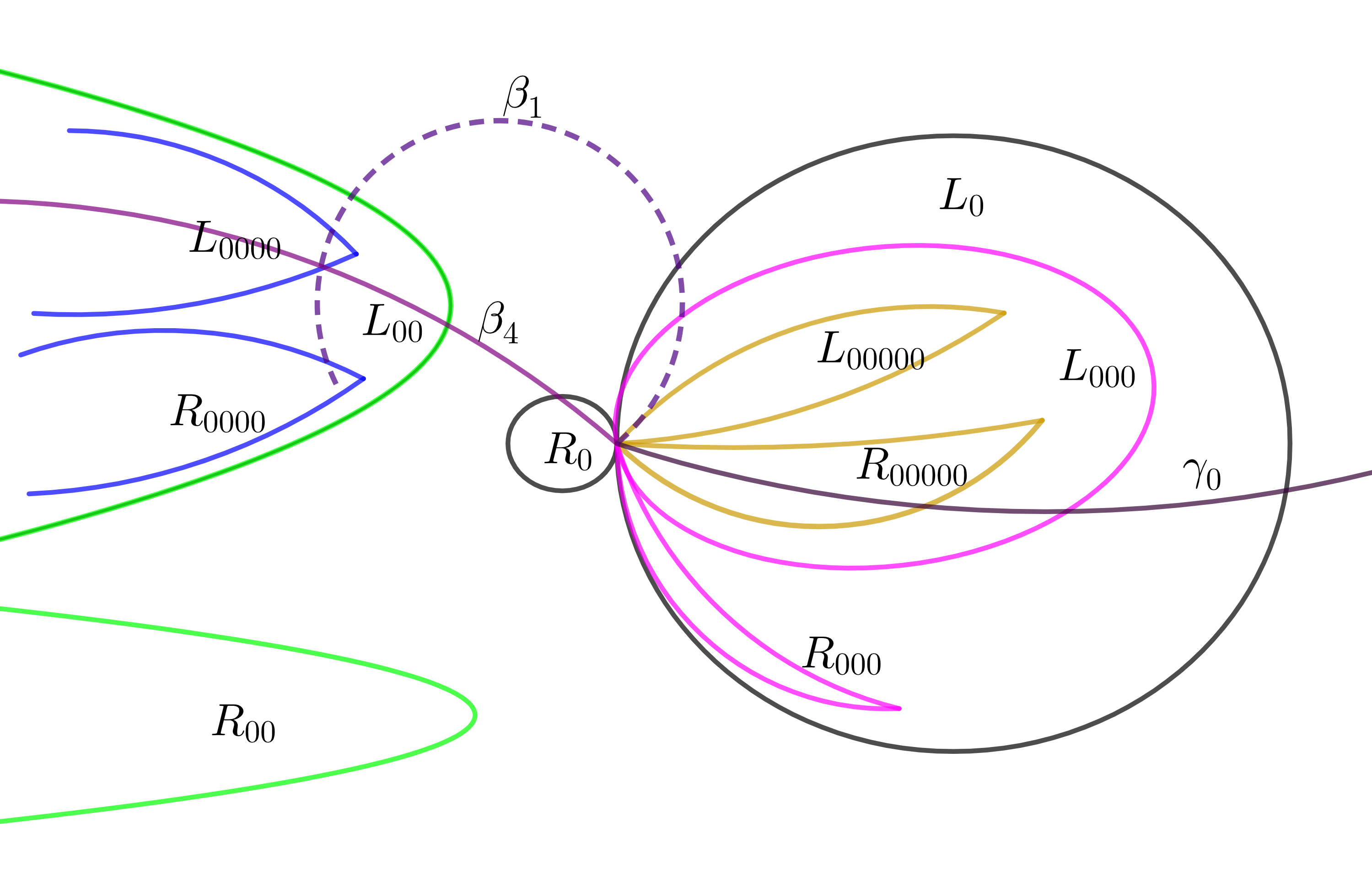
Figure 1. A period $5$ example that shows the kneading sequence cannot be $*0000$.

We next claim $k_{n-2j}\neq 0$ for some $j=1,\ldots(n-1)/2$. By proposition 4.6, we can choose $\gamma_{0}$ such that the part of $\gamma_{0}$ in $L_{0}$ approaches $0$ through $R_{k_{1}0\cdots 0k_{n-2}0}$. Pulling back, $\beta_{n-1}$ in $A_{n-1}$ goes from $L_{k_{2}0\ldots k_{n-2}0}\subset L_{00}$ to $R_{0}$. By remark 3.2, the region $L_{00}$ contains a segment of ${\mathbb{R}}^{-}$ and the argument of $\lambda$ determines whether $R_{00}$ is above or below $L_{00}$. Pulling back the vertical direction to $0$, the relative order of the regions $R_{00\ldots 0}$ and $L_{00\ldots 0}$, where the number of zeros is between $1$ and $n-1$, is unchanged. Suppose for argument’s sake that $L_{00}$ lies above $R_{00}$ as in figure 1. Otherwise the figure is reflected in the real axis. On the left, the $L_{0\ldots 0}$ have an even number of indices and are nested, converging onto a segment of ${\mathbb{R}}^{-}$. The region $R_{0\ldots 0}$ with $2j$ zeros lies below the region $L_{0\ldots 0}$ with $2j$ zeros and inside the region $L_{0\ldots 0}$ with $2j-2$ zeros.

If all the $k_{n-2j}$ were $0$, $\gamma_{0}$ would go from $R_{00\ldots 00}$ to $R$, where the number of $0$’s is $n-1$. Similarly $\beta_{n-1}$ would start in $L_{00\ldots 0}$, where the number of $0$’s is $n-2$ and end in $R_{0}$. Thus the union of the curves $\gamma_{0}\cup\beta_{n-1}$ would divide the plane. In particular, on the left it would separate the regions $R_{0\cdots 0}$, with $n-1$ $0$’s and $L_{0\cdots 0}$, with $n$ $0$’s. Since proposition 4.6 implies both these regions are in $A_{1}$, the assumption all $k_{n-2j}=0$ implies $A_{1}=A_{n-1}$ and $n=2$, a contradiction. Therefore one of the $\beta_{n-2j}$ even must join $-\infty$ to the non-zero pole $k_{n-2j}\pi i$. ∎

The following lemma will be proved in section 5.3 but we state it here to complete the ideas of this section.

Lemma 4.8.

If $n=2m$, $m>0$, the kneading sequence cannot have the form $S(\lambda)=*0k_{2}0\ldots 0k_{2m-2}0$; in particular, if $n=2$, $S(\lambda)=*k_{1}$, $k_{1}\neq 0$. In particular, if $n=2$, the kneading sequence must be $*k$ with $k\neq 0$.

Lemma 4.9.

Assume now that $n>2$ and $0\notin\partial A_{0}$. If the kneading sequence of $f_{\lambda}$ is $S(\lambda)=*k_{1}\cdots k_{n-1}$ we have the following dichotomy:

1. Either $k_{n-1}\neq 0$ and there is a unique prepole on the boundary of $A_{1}$ whose order is $n-1$ and whose address is $k_{1}\cdots k_{n-1}$,

2. Or $k_{n-1}=0$ and there is a largest integer $l$, $1\leq l<n-2$, such that $k_{l},k_{l+1}\neq 0$.

   $$S(\lambda)=*k_{1}\cdots k_{l}k_{l+1}0\cdots k_{n-2}0$$

   where $k_{l+2}=0$ and $k_{n-1}=0$.

   There is a unique prepole of lowest order on the boundary of $A_{1}$; its order is $l$ and its address is $k_{1}\cdots k_{l}$. There are also unique prepoles of order $l-j$ on $\partial A_{j+1}$ with address $k_{1}\cdots k_{l-j}$ and there are infinitely many prepoles on the boundary of $A_{0}$ of order $n-l-1$ but not any prepoles of lower order.

In both cases, $A_{1}$ is bounded.

Proof.

As in the proof of lemma 4.7, we argue by going backward around the cycle. If $k_{n-1}\neq 0$, the pole $p_{k_{n-1}}\in\partial A_{n-1}$ and $F_{k_{n-1}}(\partial A_{0})$ is bounded as $0\notin\partial A_{0}$. Therefore, the rest of the Fatou components in the cycle except $A_{0}$ are bounded. The boundary point $k_{n-1}\pi i$ on $\partial A_{n-1}$ is the only pole on the boundary of the whole immediate basin. Its preimages are the pre-poles of lowest order on the respective pullbacks. Thus the pole of lowest order on $\partial A_{1}$ has address $k_{1}\cdots k_{n-1}$.

Now suppose $k_{n-1}=0$ so that the pole on $\partial A_{n-1}$ is $0$. Then, $R_{k_{2}0}\subset A_{n-2}$, it is unbounded, and there is a pole $p_{k_{n-2}}\in\partial A_{n-3}$. If this pole is not zero, as above $A_{n-3}$ is bounded as are all its preimages. The pullbacks of $p_{k_{n-2}}$ to $A_{0}$ are prepoles of order $n-3$ and the sequence of pullbacks gives the address. If the pole is zero, $A_{n-4}$ is unbounded and we repeat the argument. Continuing in this way until we reach a non-zero pole, every other index is $0$. If no two adjacent indices were non-zero, we would never reach a non-zero pole, the sequence would be $*0k_{2}0\cdots k_{n-2}0$ and the period would be even. As we saw in lemma 4.8, this cannot happen, so there must be two adjacent non-zero indices, $k_{l},k_{l+1}$. ∎

The cases described in these lemmas lead us to make the following definitions:

Definition 8.

Let $f_{\lambda}$ be pseudo-hyperbolic and assume its immediate basin has kneading sequence $S(\lambda)=*k_{1}\cdots k_{n-1}$.

1. If $k_{n-1}\neq 0$, $S(\lambda)$ is called a regular sequence and $f_{\lambda}$ is called regular pseudo-hyperbolic.

2. If $S(\lambda)=*k_{1}0\cdots k_{n-2}0$, $n$ is odd and all the even entries are $0$, $S(\lambda)$ is called a unipolar sequence and $f_{\lambda}$ is called unipolar pseudo-hyperbolic.

3. If $S(\lambda)=*k_{1}\cdots k_{l}k_{l+1}0\cdots k_{n-2}0$, $l>1$, $k_{l},k_{l+1}\neq 0$, $S(\lambda)$ is called a hybrid sequence and $f_{\lambda}$ is called hybrid pseudo-hyperbolic.

The lemmas above show that if $\lambda$ is pseudo-hyperbolic and $n>1$, not all entries in the kneading sequence can be zero and that if $n$ is even, the sequence cannot have the form $*0k_{2}0\ldots 0k_{n-1}0$. Thus we have

Definition 9.

A kneading sequence is allowable, if it is of one of the above forms. In particular, if $n>1$, not all entries in the kneading sequence can be zero and if $n$ is even, the sequence cannot have the form $*0k_{2}0\ldots 0k_{n-1}0$.

The two lemmas immediately imply

Theorem 4.10 (Theorem B).

Let $f_{\lambda}$ be a pseudo-hyperbolic map whose attracting cycle has period $n$. Then it has a unique kneading sequence $S(\lambda)=*k_{1}\cdots k_{n-1}$ that is either regular, unipolar or hybrid.

Remark 4.2.

In the dynamics of regular pseudo-hyperbolic maps the polar asymptotic value $0$ is not on the boundary of any of the components of the immediate basin. It is therefore similar to the dynamics of hyperbolic maps investigated in earlier work on purely meromorphic functions, all of whose asymptotic values are finite, see [KK, DK, FK, CJK1, CJK2, CJK2, CK1, CK2]. This is not true for unipolar pseudo-hyperbolic maps since $0$ is always on the boundary of $A_{n-1}$. For these maps, the dynamics also exhibit properties similar to those of exponential maps (see e.g. [DFJ, S]); note that for these exponential maps, one asymptotic value is infinity — and thus a pole of order $0$. This similarity is particularly evident when the sequence is unipolar. In our discussion of parameter space below, it will be useful to separate the unipolar from the regular and hybrid cases.

4.2. Examples

In this section we show examples of the dynamical plane for functions with each of the types of kneading sequences. In figure 2, the figure on the left is for a period 1 function with $S(\lambda)=*$ and the figure on the right is in a regular period 5 component with kneading sequence $*1211$. Figure 3 shows two period 5 examples; on the left is a unipolar example with kneading sequence $*0020$ and on the right is a hybrid example with sequence $*1110$.

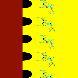
(a) Regular Period $1$                               

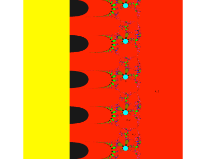
(b) Regular Period $3$

Figure 2.

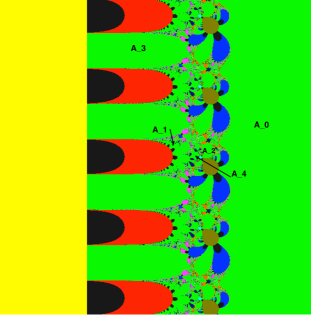
(a) Unpolar period $5$

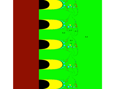
(b) Hybrid period $5$

Figure 3.

5. The Parameter plane of $\mathcal{FP}_{2}$

We now turn our attention to how the dynamics change as we vary the parameter $\lambda\in\mathbb{C}^{*}$. Note that $\lambda=0$ is a singularity since $f_{\lambda}$ is not defined.

Lemma 5.1.

The parameter space is symmetric with respect to the real line.

Proof.

It is easy to check that

$$\overline{f_{\lambda}(z)}=f_{\overline{\lambda}}(\overline{z}),$$

that is $f_{\lambda}(z)$ and $f_{\overline{\lambda}}(z)$ are conjugate. ∎

In section 3.1 we saw that there are functions in $\mathcal{FP}_{2}$ for which the asymptotic value $\lambda$ is a prepole and is thus part of a regular or hybrid virtual cycle. They are of particular interest in our study of the parameter plane so we give them a name.

Definition 10.

If the asymptotic value $\lambda^{*}$ of $f_{\lambda^{*}}$ is a prepole, and hence part of a regular or hybrid virtual cycle, we call $\lambda^{*}$ a virtual cycle parameter.

5.1. Pseudo-hyperbolic components

Although there are no hyperbolic maps in $\mathcal{FP}_{2}$, like the tangent family studied in [KK] or the families studied in [ABF, CK1, FK], the parameter space contains open sets of topologically conjugate pseudo-hyperbolic maps separated by a bifurcation locus. In the earlier work, [ABF, FK], the hyperbolic components that are universal covering maps of the punctured disk under the multiplier map are called shell components because of their shape; and their properties were studied in detail. The family $\mathcal{FP}_{2}$ is an example of what was called an exceptional family in [ABF] because one of the polar asymptotic value.

Since functions in ${\mathcal{FP}}_{2}$ do not have critical points, the multiplier map which maps the multiplier of the attracting cycle of a point in a pseudo-hyperbolic component into the unit disk cannot take the value $0$.

Definition 11.

Let $\mathcal{H}_{n}$ be the set of all $\lambda$ such that $f_{\lambda}$ has an attracting cycle of period $n$ and denote any connected subset of $\mathcal{H}_{n}$ by $\Omega_{n}$. We call the component $\Omega_{n}$ of pseudo-hyperbolic maps a shell component.

The proof of the following proposition is identical to the proof in [FK]. Since it uses standard techniques involving quasiconformal surgery on the basin of attraction of the attracting cycle we omit it.

Proposition 5.2.

Suppose $\lambda_{0}\in\mathcal{H}_{n}$. Then there is a neighborhood $U$ of $\lambda_{0}\in{\mathbb{C}}^{*}$ such that if $\lambda\in U$, $f_{\lambda}$ is pseudo hyperbolic with attracting cycle of period $n$; that is any component $\Omega_{n}$ is open. Moreover, all the maps in a given component are quasi-conformally and hence topologically conjugate.

This says that the pseudo-hyperbolic maps in a given component have the same dynamics and, in particular, that they all share the same kneading sequence.

Definition 12.

The bifurcation locus ${\mathcal{B}}={\mathcal{B}}(\mathcal{FP}_{2})$ is the set of parameters that are not structurally stable.

By the proposition above, ${\mathcal{B}}$ is contained in the complement of $\cup_{n}\mathcal{H}_{n}$.

By theorem 6.4 and its corollary 6.5, and by theorem 6.13 in the paper [FK], the multiplier map $m:\Omega_{n}\rightarrow{\mathbb{D}}^{*}$ that assigns the multiplier $m(\mathbf{z}_{\lambda})=\Pi_{i=0}^{n-1}f_{\lambda}^{\prime}(z_{i}(\lambda))$ to the cycle $\mathbf{z}_{\lambda}=\{z_{0}(\lambda),\ldots z_{n-1}(\lambda)\}$ is a universal covering map. It extends continuously to the boundary.

The boundary of $\Omega$ is analytic along curves where $m(\mathbf{z}_{\lambda})=e^{i\theta}$, $\theta\neq 2\pi k$ for any integer $k$ and it has a cusp if $\theta=2\pi k$. It is this property of the component that gives it the appearance of a shell, hence the name.

The universal cover is conformally equivalent to a half plane so that $\Omega$ is simply connected. It therefore has a unique boundary point corresponding to the point at infinity on the boundary of this half plane. This is a point where the boundary is non-analytic and we give it a name.

Definition 13.

Let $\lambda_{n}$ be a sequence of points in $\Omega_{n}$ such that $\lim_{n\to\infty}\lambda_{n}=\lambda^{*}\in\partial\Omega_{n}$ or $\lim_{n\to\infty}\lambda_{n}=\infty\in\partial\Omega_{n}$ and suppose $\lim_{n\to\infty}m(\mathbf{z}_{\lambda_{n}})=0$. Then the boundary point $\lambda^{*}$ or infinity is called a virtual center of $\Omega_{n}$.

It follows from proposition 5.2 that the parameters in a given $\Omega$ are either all regular pseudo-hyperbolic or all unipolar pseudo-hyperbolic or all hybrid pseudo-hyperbolic. We therefore define

Definition 14.

If $\Omega$ is a shell component containing regular parameters we call it a regular shell component, (or just a regular component); if $\Omega$ is a shell component containing unipolar parameters we call it a unipolar shell component, or just a (unipolar component) and if $\Omega$ is a shell component containing hybrid parameters we call it a hybrid shell component, (or just a hybrid component).

Figure 4 depicts the parameter plane. The black and white regions correspond to round-off errors. The large component on the right (yellow) is $\Omega_{1}$. The unbounded components on the left are the unipolar components. The largest (red) are period $3$ and the next largest, between the period $3$’s are period $5$’s (bright green). The bounded bulb-like components tangent to $\Omega_{1}$ are regular components of varying periods: the largest (cyan) are period $2$, the next smaller ones are period $3$ red, and so on.

Figure 5 shows two different blow-ups of areas of figure 4. On the left in we have zoomed in near $0$ and we see period $3$ unipolar components at the top and bottom left. The unipolar period $5$ components are more visible here, as are the period $7$’s (dark blue) between them and the period $9$’s (orange) between the $7$’s. On the right we have zoomed in on the period $2$ component with virtual center at $\pi i$. The largest hybrid components of period $4$ (khaki) that share this virtual center are now visible and there are period $6$ (royal blue) components visible between them. There are also regular period $4$ and $6$ components budding off of the period $2$ component.

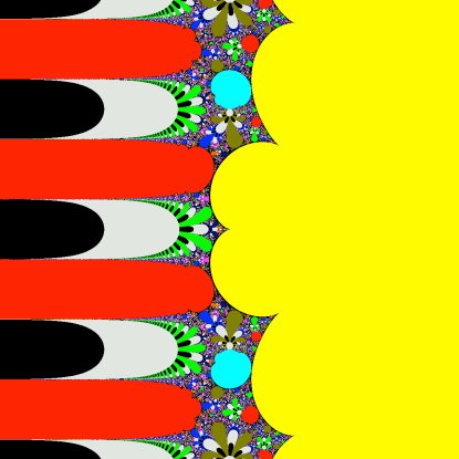
Figure 4. The parameter plane

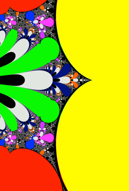
(a) zoom in near $0$

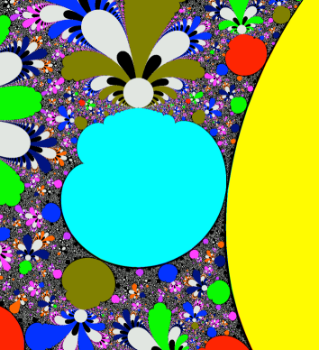
(b) Zoom in near $\pi i$

Figure 5.

The following proposition except for case (3c) was proved in [FK] as proposition 6.8 and the proof goes through here without modification.

Proposition 5.3.

Suppose $\Omega$ is a shell component of period $n\geq 1$ and let $\lambda_{k}$ be a sequence of points in $\Omega$ such that $\lim_{k\to\infty}\lambda_{k}=\lambda^{*}\in\partial\Omega\cap\widehat{\mathbb{C}}^{*}$. Let $\mathbf{z}^{k}=\{z_{0}^{k},\ldots,z_{n-1}^{k}\}$ be the periodic cycle of $f_{k}=f_{\lambda_{k}}$ attracting $\lambda_{k}$.

1. If the cycle $\mathbf{z}^{k}$ stays bounded as $k\to\infty$, then $f_{\lambda^{*}}$ has an indifferent periodic cycle $\mathbf{z}^{*}$ whose period divides $n$ and $\mathbf{z}^{k}\to\mathbf{z}^{*}$.

2. If $n=1$, and $|z_{0}^{k}|\to\infty$ as $k\to\infty$, then $\Re z_{0}^{k}\to+\infty$, $\lambda_{k}\to+\infty$ and $m(\mathbf{z}^{k})\to 0$.

3. If $n>1$ and $|z_{j}^{k}|\to\infty$ as $k\to\infty$ for some $0\leq j<n$, then

   1. If $\Omega$ is a regular component, $f_{\lambda^{*}}^{j-1}(\lambda^{*})$ is a non-zero pole and $j=n$.

   2. If $\Omega$ is a hybrid component, $j$ is the smallest index such that $f_{\lambda^{*}}^{j-1}(\lambda^{*})=k_{l}\pi i$ where $n=j+2m$ and $k_{l}\neq 0$ is defined in definition 8; thus, $k_{l}=k_{n-j}$.

   3. If $\Omega$ is a unipolar component, $\Re\lambda\rightarrow-\infty$, $n=2m+1$, $j$ is odd and the limit cycle is $\{+\infty,-\infty,0,-\infty,\ldots,-\infty,0\}$.

In cases (3a) and (3b) $\lambda^{*}$ is a virtual cycle parameter as well as a virtual center. In case (3a) its address is given by the sequence and in case (3b) its address is given by the first part of the sequence, $k_{1}\ldots k_{l}$. In case (3c), we don’t have a virtual cycle because $\lambda^{*}$ is the parameter singularity $\infty$. As $\lambda$ tends to $\infty$ in the unipolar component, the immediate basin of $f_{\lambda}$ contains a cycle of paths with endpoints on the boundary. All the odd components but the last contain a path in the left half plane tending to $-\infty$, all the even components contain a path ending at $0$ and $A_{0}$ contains a path in the right half plane whose endpoint is $+\infty$.

Proof of (3c).

By definition if $\lambda$ is in a unipolar component it has kneading sequence $*k_{1}0\cdots 0k_{n-2}0$. From the proof of lemma 4.7 it follows that $A_{j}^{k}$ is unbounded in the left half plane for all odd $j$. Therefore if $|z_{j}^{k}|\to\infty$, $\Re z_{j}^{k}\to-\infty$ and $z_{j+1}^{k}\to 0$. Moreover, $z_{j-1}^{k}$ tends to a pole. If the pole is not $0$, $\lambda$ is not in a unipolar component so the pole is zero and $|z_{j-2}^{k}|\to\infty$. Continuing to pull back around the cycle we get $\Re z_{1}^{k}\to-\infty$ and $\Re z_{0}^{k}\to+\infty$. ∎

This proposition and lemma 6.9 in [FK] quoted above imply

Theorem 5.4 (Theorem C).

If $\Omega$ is a pseudo-hyperbolic shell component of ${\mathcal{FP}}_{2}$ and $\lambda^{*}\in\partial\Omega$ is its virtual center, then $\lambda^{*}$ is a virtual cycle parameter.

In the next section we prove that the converse holds: we construct shell components at each virtual cycle parameter and these are their virtual centers.

5.2. The set $\mathcal{H}_{1}$

Theorem 5.5.

The set $\mathcal{H}_{1}$ consists of a single connected component $\Omega_{1}$ which is an unbounded simply connected open set contained in the right half plane. It does not, however, contain any bi-infinite vertical strip. The point $+\infty$ acts as its virtual center.

See the component on the right in figure 4.

Proof.

For any $\lambda$, any fixed point $z=z(\lambda)$ of the map $f_{\lambda}$ satisfies the equation

$$\frac{\lambda}{1-e^{-2z}}=z$$

and its multiplier is

$$m=m(z)=m(z(\lambda))=\frac{-2\lambda e^{-2z}}{(1-e^{-2z})^{2}}=\frac{-2ze^{-2z}}{1-e^{-2z}}.$$

It is easy to check that

$$\lim_{\Re z\to+\infty}\frac{-2ze^{-2z}}{1-e^{-2z}}=0$$

and

$$\lim_{\Re z\to-\infty}\frac{-2ze^{-2z}}{1-e^{-2z}}=\infty.$$

Therefore $m(z)$ has two asymptotic values, $0$ and $\infty$, each with a single asymptotic tract in the right and left half planes respectively. It follows that $m^{-1}({\mathbb{D}}^{*})$ is a simply connected set in a right half plane; that is, there is a $B\in{\mathbb{R}}$ such that $m^{-1}({\mathbb{D}}^{*})\subset\{\Re z>B\}$.

We claim the intersection of any vertical line and $m^{-1}(\mathbb{D}^{*})$ is contained in a finite segment of the line. To see this, set $z=z(\lambda)=M+iy$ and let $M>0$; then for small $|y|$,

$$|m|=|\frac{-2ze^{-2z}}{1-e^{-2z}}|\leq\frac{|2z|e^{-2M}}{1+e^{-2M}}<1$$

and for large for $|y|$,

$$|m|=|\frac{-2ze^{-2z}}{1-e^{-2z}}|\geq\frac{|2z|e^{-2M}}{1-e^{-2M}}>1.$$

This implies that $m^{-1}({\mathbb{D}}^{*})\cap\{z=M+iy\}$ is contained within a finite line segment.

Finally, since $\lambda=z(1-e^{-2z})$ and

$$\frac{\lambda}{z}=1-e^{-2z}\to 1,$$

as $\Re z\to\infty$, the real parts of both the fixed point and $\lambda$ tend to $+\infty$. Thus $\Omega_{1}$ is contained in, but does not contain any full right half plane.

It has a boundary point at $+\infty$ where the limit of $m$ is zero, so this acts like a virtual center. Because $0$ is an omitted value for $m$, at any finite boundary point the multiplier is non-zero and therefore there is no finite virtual center. ∎

Remark 5.1.

Suppose $z=iy$ is a fixed point. Then

$$|m|^{2}=\frac{4y^{2}}{2-2\cos(2y)}=\frac{y^{2}}{\sin^{2}y}\geq 1,$$

so the fixed point cannot attract $\lambda$. Since the fixed point is a holomorphic function of $\lambda$, it follows that if $z$ is an attracting fixed point, it must be in the right half plane. On the left in figure 5, $\Omega_{1}$ is the large domain on the right. Close to the cusp boundary point at $0$, there are clearly points $\lambda\in\Omega_{1}$ with $\Re\lambda<0$. By the above, however, the fixed points corresponding to such $\lambda$’s are in the right half plane.

Lemma 5.6.

The positive real line $\lambda=x,x>0$ is contained in $\Omega_{1}$.

Proof.

For any real $\lambda>0$,

$$\lim_{x\to 0^{+}}f_{\lambda}(x)=\infty\mbox{ and }\lim_{x\to\infty}f_{\lambda}(x)=\lambda.$$

Therefore the equation $f_{\lambda}(x)=x$, written out as

$$\frac{\lambda}{1-e^{-2x}}=x,$$

always has a positive solution. Rewriting as $\lambda=x(1-e^{-2x})$, we see that the fixed point $x$ is increasing with respect to $\lambda$. In particular, $x\to 0$ as $\lambda\to 0^{+}$ and $x\to\infty$ as $\lambda\to\infty$.

As above, the multiplier of the fixed point is

$$\frac{-2\lambda e^{-2x}}{(1-e^{-2x})^{2}}=\frac{-2xe^{-2x}}{1-e^{-2x}}.$$

It tends to $-1$ as $x\to 0^{+}$ and to $0$ as $x\to\infty$. ∎

Remark 5.2.

On the positive real line, the multiplier of the fixed point is between $0$ and $-1$. In particular, the multiplier approaches $-1$ as $\lambda$ approaches $0$. There is, however, no period doubling at $0$ at this point because it is a singularity of the parameter space.

5.3. No virtual center at $0$

From theorem C, there is a virtual cycle parameter which is a pole of order $1$ on the boundary of each component in $\mathcal{H}_{2}$, so it is the point $\pi ik$ for some $k\in{\mathbb{Z}}$. That is, it is a solution to $f_{\lambda}(\lambda)=\frac{\lambda}{1-e^{-2\lambda}}=\infty$. There is also a virtual cycle parameter at each hybrid component where the address of the pole is $k_{1}\ldots k_{l}$.

Note that $\lim_{\lambda\to 0}\frac{\lambda}{1-e^{-2\lambda}}=1/2$, so that zero cannot be a virtual center parameter, even as a limit, and therefore it cannot be a virtual cycle parmeter. Thus we have

Lemma.

4.8 There is no pseudo-hyperbolic $f_{\lambda}$ whose kneading sequence has the form $*0$ or $*0k_{2}0\cdots k_{n-2}0$.

Proof.

If there were such an $f_{\lambda}$, it would be in a component whose virtual center would be $0$ and we saw above that cannot happen. ∎

An immediate corollary is

Corollary 5.7.

The kneading sequence of every pseudo-hyperbolic map is an allowable sequence.

In the next section we will show that for any integer $k$, $k\neq 0$, there is a regular shell component whose kneading sequence is $*k$.

5.4. The set $\mathcal{H}_{n}$

The injective inverse branches of $f_{\lambda}$ defined by going backwards $n-1$ times from the component containing $\lambda$ around a periodic $n$ cycle always depend holomorphically on $\lambda$. This immediately proves

Proposition 5.8.

If $n\geq 2$, every attracting cycle of $f_{\lambda}$ in a fixed component $\Omega_{n}$ has the same kneading sequence.

Therefore, we may identify the kneading sequence of any one of these cycles with the component and set $S(\Omega)=*k_{1}\cdots k_{n-1}$.

6. Existence of pseudo-hyperbolic components

In this section we give a full description of how the pseudo-hyperbolic components in the parameter plane are situated. In particular, we prove that every virtual cycle parameter is the virtual center of one regular and infinitely many hybrid pseudo-hyperbolic components. We also show that there are components corresponding to all allowable kneading sequences.

Theorem 6.1 (Theorem D).

Given any allowable kneading sequence $S=*k_{1}k_{2}\ldots k_{n-1}$ with $n>1$:

1. If $S$ is a unipolar sequence, $S=*k_{1}0\cdots 0k_{n-2}0$, $n$ is odd and there is a unipolar pseudo-hyperbolic component associated to it. This component is unbounded in the left half plane and, as $\Re{\lambda}\to-\infty$ in the component, the multiplier of the attracting cycle goes to $0$.

2. If $S$ is a regular sequence, $S=*k_{1}\cdots k_{n-1}$, where $k_{n-1}\neq 0$, then there is a regular component associated it, and its virtual center is the virtual cycle parameter with the same address.

3. If $S$ is a hybrid sequence, $S=*k_{1}\cdots k_{l-1}k_{l}k_{l+1}0\cdots k_{n-2}0$, then the first part of sequence, $k_{1}\cdots k_{l},$ is the address of a regular virtual cycle parameter and there is a hybrid component whose virtual center is this virtual cycle parameter and it has kneading sequence $S$.

Note that a regular sequence may have an even period. Since there are infinitely many kneading sequences that share a given first part, corollary of this theorem is

Corollary 6.2.

There are infinitely many hybrid components that share a virtual center with one regular component.

Remark 6.1.

Although infinity is not a parameter, it is a boundary point of infinitely many components for which it acts as a virtual center: the regular period $1$ component whose kneading sequence $*$ contains no first part and the infinitely many pure unipolar components that are defined by sequences that consist only of the pole followed by alternating $0$’s.

We prove each part of the theorem separately. The proof of the first part takes advantage of the fact that, restricted to neighborhoods of $0$ and $\infty$, the second iterate of a map in ${\mathcal{FP}}_{2}$ acts like an exponential map and the structure of the unipolar pseudo-hyperbolic components is reminiscent of the structure of the hyperbolic components of exponential maps described in [DFJ, S]. The proof of the second part is very similar to the proof of Theorem B in [CK1] in which the dynamics of a function whose asymptotic value is a prepole is perturbed. The proof of the third part combines techniques in the first two.

6.1. Proof of theorem 6.1 part $(1)$: unipolar maps

It follows from proposition 4.6 and lemma 4.7, that to prove the existence of a $\lambda$ with the given kneading sequence $*k_{1}0\cdots 0k_{n-2}0$ we need to show there is a $\lambda$ such that in the L-R structure of $f_{\lambda}$, $\lambda\in R_{k_{1}0\ldots k_{n-2}0}(\lambda)$. For such a $\lambda$,

$$R_{k_{1}0\cdots 0k_{n-2}0}(\lambda)\subset L_{k_{1}0\cdots 0k_{n-4}0}(\lambda)\subset L_{k_{1}0\ldots 0k_{n-6}0}(\lambda)\cdots\subset L_{k_{1}0}(\lambda)\subset L$$

so that $f_{\lambda}^{n-1}(\lambda)$ is contained in a right half plane; it is clear, that $n-1$ must be even.

We will need the basic estimates in  (1) for the exponential map which we will use to follow the orbit of $\lambda$.

To construct the pseudo-hyperbolic components we proceed inductively. The first step is to construct a component of period $3$ with $S(\lambda)=*k0$. Since we have assumed the sequence is allowable, $k\neq 0$. We first construct a “candidate” strip using the estimates above. Then we prove that for $\lambda$ in that strip, $f_{\lambda}$ has an attracting cycle of period $3$.

We have seen that the parameter space is symmetric about the real axis and that there is an infinite segment of the positive real axis contained in a period $1$ component. In this proof we will consider strips about the lines whose imaginary parts are odd multiples of $\pi$. In order to keep the labeling consistent with the symmetry, and because $k\neq 0$, we will label these lines by $2k-1$ in the upper half plane where $k>0$ and by $2k+1$ in the lower half plane where $k<0$.

Theorem 6.3.

Given the kneading sequence $S(\lambda)=*k0$, $k\neq 0$, there exists a large $M>0$ and a small $\epsilon>0$ such that if $-2\lambda$ is in the half strip of the right half plane centered along the line whose imaginary part is an odd multiple of $\pi$, that is, for $k>0$

$$-2\lambda\in{\mathcal{R}}_{k,M,\epsilon}^{odd}=\{z=x+iy\ |\ x>M,(2k-1)\pi-\frac{\pi}{2}+\epsilon<y<(2k-1)\pi+\frac{\pi}{2}-\epsilon\},$$

and for $k<0$

$$-2\lambda\in{\mathcal{R}}_{k,M,\epsilon}^{odd}=\{z=x+iy\ |\ x>M,(2k+1)\pi-\frac{\pi}{2}+\epsilon<y<(2k+1)\pi+\frac{\pi}{2}-\epsilon\},$$

then $f_{\lambda}$ has an attracting cycle of period $3$ with the given kneading sequence.

Proof.

Set $w_{0}=\lambda$ and $w_{n}=f_{\lambda}^{n}(\lambda)$, $n=1,2,\cdots$. Note that each $w_{n}$ is a holomorphic function of $\lambda$. Using the estimates above, if for $M$ large enough, $-2\lambda\in{\mathcal{R}}^{odd}_{k,M,\epsilon}$ then

$$w_{1}=\frac{\lambda}{1-e^{-2\lambda}}\sim-\frac{\lambda}{e^{-2\lambda}}\sim 0$$

so that

$$w_{2}=\frac{\lambda}{1-e^{-2w_{1}}}\sim\frac{\lambda}{2w_{1}}\sim-\frac{e^{-2\lambda}}{2}$$

and for small $\epsilon$, $\Re w_{2}>e^{M}\sin\epsilon$.

Choose and fix a $\lambda$ such that $-2\lambda\in{\mathcal{R}}^{odd}_{k,M,\epsilon}$ and consider its dynamic plane. We will show $f_{\lambda}$ has an attracting period $3$ cycle. Let $U_{2}=\{z\ |\ \Re z>\Re w_{2}-1\}$, $U_{1}$ the component of $f^{-1}_{\lambda}(U_{2})$ containing $w_{1}$, and $U_{0}$ the component of $f^{-1}_{\lambda}(U_{1})$ containing $\lambda$; then $0\in\partial U_{1}$. Since $f^{2}_{\lambda}:U_{0}\to U_{2}$ is conformal, its inverse is well-defined; denote it by $h_{1}$. By the Koebe $1/4$ theorem,

$$dist(\lambda,\partial U_{0})\geq\frac{|h^{\prime}_{1}(w_{2})|}{4} =\frac{1}{4}\frac{1}{|f^{\prime}_{\lambda}(w_{1})|}\frac{1}{|f^{\prime}_{\lambda}(\lambda)|}$$

$$=\frac{1}{4}\frac{|(1-e^{-2w_{1}})^{2}|}{|\lambda e^{-2w_{1}}|}\frac{|(1-e^{-2\lambda})^{2}|}{|\lambda e^{-2\lambda}|}$$

$$\sim\frac{1}{4}\frac{|4w_{1}^{2}|}{|\lambda|}\frac{|(1-e^{-2\lambda})^{2}|}{|\lambda e^{-2\lambda}|}=|\frac{w_{1}^{2}(1-e^{-2\lambda})^{2}}{\lambda^{2}e^{-2\lambda}}|=|e^{2\lambda}|$$

Furthermore, for any $z\in U_{2}$,

$$|f_{\lambda}(z)-\lambda|=\frac{|\lambda e^{-2z}|}{|1-e^{-2z}|}<\alpha e^{2}|\lambda e^{-2w_{2}}|\sim\alpha e^{2}|\lambda e^{-e^{-2\lambda}}|$$

for some positive constant $\alpha<2$ depending on $M$ and $\epsilon$.

Choosing $M$ and $\epsilon$ respectively large and small enough, we can assure that $w_{2}>>0$ and $|e^{2\lambda}|>\alpha e^{2}|\lambda e^{-e^{-2\lambda}}|$ so that $f_{\lambda}^{3}(U_{0})$ is properly contained in $U_{0}$. Therefore by the Schwarz lemma, there is an attracting cycle in $U_{0},U_{1},U_{2}$ and the set $R_{k0}$ of the L-R structure for $f_{\lambda}$ is contained in $U_{0}$. ∎

It follows that for all $M^{\prime}>M$ and $\epsilon^{\prime}>\epsilon$, there is a unipolar pseudo-hyperbolic component of period $3$ with kneading sequence $*k0$. Moreover, for each $\lambda$ such that $-2\lambda\in{\mathcal{R}}^{odd}_{M,k,\epsilon}$, if $k>0$, the set $R_{k0}(\lambda)$ of the L-R structure of the dynamic plane $f_{\lambda}$ is contained in the left half strip

$${\mathcal{L}}_{M/2,\epsilon,k}=\{z=x+iy\,|\,x<-M/2,k\pi-\frac{3\pi}{4}+\epsilon<y<k\pi+\frac{\pi}{4}-\epsilon\}$$

and for $k<0$ it is contained in the left half strip

$${\mathcal{L}}_{M/2,\epsilon,k}=\{z=x+iy\,|\,x<-M/2,k\pi+\frac{\pi}{4}+\epsilon<y<k\pi+\frac{3\pi}{4}-\epsilon\}.$$

Since the strips are open, $\cap R_{k0}(\lambda)\neq\emptyset$ and the intersection is contained in the asymptotic tract of $0$ for each $f_{\lambda}$. It follows that we can identify this intersection with a neighborhood of infinity in the parameter plane ${\mathbb{C}}$ and this neighborhood is contained in a period $3$ pseudo-hyperbolic component.

To prove theorem 6.1 part $(2)$ for all kneading sequences $S=*k_{1}0\ldots k_{n-2}0$, we generalize the construction above. Because the period is odd, we set $n=2m+1$. Then, using the kneading sequence, we create pairs of disjoint strips in the left and right half planes where again $\lambda$ is in the strip in the left half plane but now $w_{2m}=f^{2m}_{\lambda}(\lambda)$ is in the strip in the right half plane.

More precisely, to find the attracting cycles of period $2m+1$, we need to look for $\lambda$’s, whose orbits $\{w_{0},w_{1},\cdots,w_{2m}\}$ satisfy

• $w_{2i-1}$, $i=1,\cdots,m$ is sufficiently close to zero,

• $w_{0},w_{2},\cdots w_{2m-2}$ are in the left plane and their real parts have sufficiently large absolute values.

• $w_{2m}$ is in the right half plane with sufficiently large real part.

To do this, we need to define a structure on the parameter plane that is analogous to the L-R structure we defined in the dynamic planes of each of the functions $f_{\lambda}$. We define strips in the right half plane centered on the lines whose imaginary parts, $2k\pi$, are even multiples of $\pi$,

$$\mathcal{R}_{k,M,\epsilon}^{even}=\{\lambda=x+iy\ |\ x>M,2k\pi-\frac{\pi}{2}+\epsilon<y<2k\pi+\frac{\pi}{2}-\epsilon\}.$$

Note that Assume $M>0$ is large and $\epsilon>0$ is small. For readability set $E(z)=e^{z}$.

The following theorem is a restatement of the first assertion in theorem 6.1 part $(1)$.

Theorem 6.4.

Given $n$ and an allowable unipolar kneading sequence $S=*k_{1}0\cdots 0k_{n-2}0$, there is a $\lambda\in{\mathbb{C}}^{*}$ such that $f_{\lambda}$ has an attracting cycle of period $n$ with this kneading sequence. In particular, there is a $\lambda$ such that for $i=1,\cdots,m-2$,

$$E^{i}(-2\lambda)\in\mathcal{R}^{even}_{k_{2i+1},M,\epsilon}$$

and

$$E^{m-1}(-2\lambda)\in\mathcal{R}^{odd}_{k_{n-2},M,\epsilon}.$$

Proof.

If $M$ is sufficiently large and $\epsilon$ is sufficiently small, by periodicity, for any $k$, $I=E({\mathcal{R}}^{even}_{k,M,\epsilon})$ is a region outside the disk $|z|<e^{M}$ and contained between the rays $te^{\pm\epsilon i}$, $t>e^{M}$. That is, it is a sector at infinity in the right half plane, symmetric with respect to the real line and lying outside the disk $|z|<e^{M}$. To insure that the disk intersects the line $\Re z=M$, we choose $\epsilon$ small enough so that $e^{M}\sin\epsilon>M$. Note that for all $k$ and $\Re z$ large enough, all the strips $\mathcal{R}^{even}_{k,M,\epsilon}$ and $\mathcal{R}^{odd}_{k,M,\epsilon}$ intersect $I$. Figure 6 illustrates this.

Note that for any $k$, and for any $\lambda$ with $-2\lambda\in\mathcal{R}_{k,M,\epsilon}^{even}$, $E(-2\lambda)\in I$; thus $w_{2}\sim-E(-2\lambda)/2$ is in the left half plane. In particular, this is true for $k=k_{1}$.

Now choose $\lambda$ so that $-2\lambda\in\mathcal{R}^{even}_{k_{1},M,\epsilon}$ and also require that its image $E(-2\lambda)$ is in $I\cap\mathcal{R}^{even}_{k_{2},M,\epsilon}$. Then,

$$w_{3}=\frac{\lambda}{1-e^{-2w_{2}}}\sim-\frac{\lambda}{e^{-2w_{2}}}\sim-\frac{\lambda}{e^{e^{-2\lambda}}}\sim 0$$

and

$$w_{4}=\frac{\lambda}{1-e^{-2w_{3}}}\sim\frac{\lambda}{2w_{3}}\sim-\frac{e^{e^{-2\lambda}}}{2}=\frac{-E^{2}(-2\lambda)}{2}.$$

As above, $E^{2}(-2\lambda)$ is contained in $I$ and $\Re E^{2}(-2\lambda)>e^{e^{M}\sin\epsilon}\sin\epsilon/2$; thus $w_{4}\sim-E^{2}(-2\lambda)/2$ is in the left half plane and even further to the left than $w_{2}$. See figure 6 again.

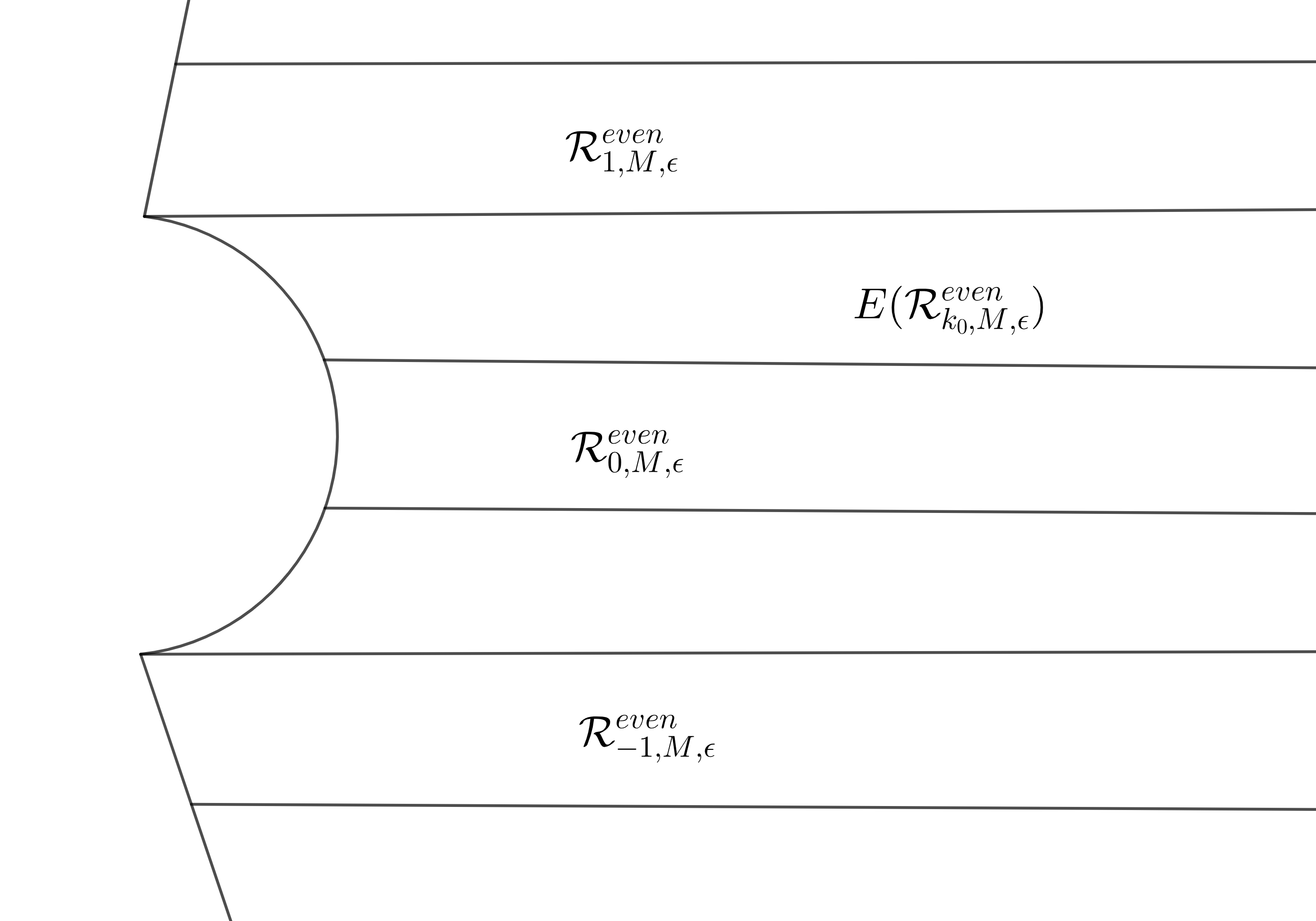
Figure 6. The intersection of the image $I$ of $E(\mathcal{R}^{even}_{k,M,\epsilon})$ for any $k$, with the strips $I\cap\mathcal{R}^{even}_{{k_{i}},M,\epsilon}$

We can iterate this procedure, choosing $\lambda$ so that for $i=1,\ldots,n-2$, the successive images $E^{i}(-2\lambda)$ lie in the strips $I\cap\mathcal{R}^{even}_{{k_{i}},M,\epsilon}$. Having done this, $w_{i}$ is in the left half plane,

$$w_{2i-1}=\frac{\lambda}{1-e^{-2{w_{2i-2}}}}\sim-\frac{\lambda}{e^{-2w_{2i-2}}}\sim-\frac{\lambda}{E^{i}(-2\lambda)}\sim 0$$

and

$$w_{2i}=\frac{\lambda}{1-e^{-2w_{2i-1}}}\sim\frac{\lambda}{2w_{2i-1}}\sim\frac{-E^{i}(-2\lambda)}{2}.$$

Now, modify the choice of $\lambda$ so that, in addition to the above, it satisfies $E^{m-1}(-2\lambda)\in\mathcal{R}^{odd}_{k_{n-1},M,\epsilon}$. Then, for such a $\lambda$, $w_{2i}\sim-E^{i}(-2\lambda)/2$, $i=0,\cdots,m-1$, is in the the left half plane, and $w_{2m}\sim-e^{E^{n-1}(-2\lambda)}/2$ is in the right half plane.

Let $\tilde{V}$ denote the set of $\lambda$’s defined by the intersection of all these regions. A $\lambda\in\tilde{V}$ is a candidate to have an attractive cycle of period $n=2m+1$. We now show it does.

Fix the candidate $\lambda$, and look at the dynamical plane of $f_{\lambda}$. Let $U_{2m}=\{z\ |\ \Re z>\Re w_{2m}-1\}$, and let $U_{2m-i}$ be the component of $f^{-i}_{\lambda}(U_{2m})$ containing $w_{i}$, for $i=1,\cdots,2m$. Then $0\in\partial U_{2i-1}$ and $U_{2i}$ is unbounded. Since $f^{2m}_{\lambda}:U_{0}\to U_{2m}$ is conformal, its inverse is well-defined; denote it by $h_{n}$. By the Koebe $1/4$ theorem,

$$dist(\lambda,\partial U_{0})\geq\frac{|h^{\prime}_{n}(w_{2m})|}{4} =\frac{1}{4}\frac{1}{|f^{\prime}_{\lambda}(\lambda)|}\frac{1}{|f^{\prime}_{\lambda}(w_{1})|}\cdots\frac{1}{|f^{\prime}_{\lambda}(w_{2m-2})|}\cdot\frac{1}{|f^{\prime}_{\lambda}(w_{2m-1})|}$$

$$=\frac{1}{4}\frac{|(1-e^{-2\lambda})^{2}|}{|\lambda e^{-2\lambda}|}\cdot\frac{|(1-e^{-2w_{1}})^{2}|}{|\lambda e^{-2w_{1}}|}\cdots\frac{|(1-e^{-2w_{2m-2}})^{2}|}{|\lambda e^{-2w_{2m-2}}|}\cdot\frac{|(1-e^{-2w_{2m-1}})^{2}|}{|\lambda e^{-2w_{2m-1}}|}$$

$$\sim\frac{1}{4}\frac{|(1-e^{-2\lambda})^{2}|}{|\lambda e^{-2\lambda}|}\frac{|4w_{1}^{2}|}{|\lambda|}\cdots\frac{|(1-e^{-2w_{2m-2}})^{2}|}{|\lambda e^{-2w_{n-2}}|}\frac{|4w_{2m-1}^{2}|}{|\lambda|}$$

$$=\frac{1}{4}\Big{|}\frac{w_{1}^{2}(1-e^{-2\lambda})^{2}}{\lambda^{2}e^{-2\lambda}}\Big{|}\cdots\Big{|}\frac{w_{2m-1}^{2}(1-e^{-2w_{2m-2}})^{2}}{\lambda^{2}e^{-2w_{2m-2}}}\Big{|}$$

$$=\frac{4^{n-1}}{|E(-2\lambda)\cdots E^{n}(-2\lambda)|}$$

Furthermore, for any $z\in U_{2m}$,

$$|f_{\lambda}(z)-\lambda|=\frac{|\lambda e^{-2z}|}{|1-e^{-2z}|}<\alpha e^{2}|\lambda e^{-2w_{2m}}|\sim\alpha e^{2}|\lambda E^{n+1}(-2\lambda)|$$

for some constant $0<\alpha<2$.

It is obvious now, that there exist $M,\epsilon>0$ and a $\lambda$ that satisfies the conditions:

$$E^{i}(-2\lambda)\in\mathcal{R}^{even}_{k_{i},M,\epsilon}\mbox{for }i=0,\cdots,n-2,$$

$$E^{n-1}(-2\lambda)\in\mathcal{R}^{odd}_{k_{n-1},M,\epsilon},$$

$$E^{i}(-2\lambda)\in\mathcal{R}^{even}_{k_{2i+1},M,\epsilon}\mbox{for }i=0,\cdots,m-2,$$

$$E^{m-1}(-2\lambda)\in\mathcal{R}^{odd}_{k_{n-2},M,\epsilon},$$

$$\Re w_{2m}>>0\mbox{ and }$$

$$\frac{4^{m-1}}{|E(-2\lambda)\cdots E^{m}(-2\lambda)|}>\alpha e^{2}|\lambda E^{m+1}(-2\lambda)|.$$

Therefore $f_{\lambda}^{2m+1}(U_{0})$ is properly contained in $U_{0}$ so by the Schwarz lemma, there is an attracting cycle in $U_{0},U_{1},\cdots,U_{2m}$.

It is clear from the construction that the set $R_{0k_{2}0\ldots 0k_{n-2}0}(\lambda)$ of the L-R structure of $f_{\lambda}$ is a subset of $U_{0}(\lambda)$ and that for these $\lambda$’s the intersection of the $R_{0k_{2}0\ldots 0k_{n-2}0}(\lambda)$ is not empty. This interesection is contained in the asymptotic tracts of $0$ for each $f_{\lambda}$. If we identify this intersection with a neighborhood of the parameter plane, we obtain an open set in a pseudo-hyperbolic component all of whose $\lambda$’s have the given kneading sequence. ∎

We have shown that there exists a unipolar parameter $\lambda=x+iy$ with an attracting cycle and given allowable kneading sequence. Let $\Omega$ denote the pseudo-hyperbolic component containing $\lambda$. From the proof, it is clear that any $\lambda^{\prime}=x^{\prime}+iy$, $x^{\prime}<x$, is in $\Omega$.

Proposition 6.5.

Suppose $\{\lambda_{j}\}\in\Omega$, with $\Re\lambda_{j}\to-\infty$ and let $m(\mathbf{z^{j}})$ be the multipler of the attracting cycle of period $2m+1$ of $f_{\lambda_{j}}$. Then $\lim_{j\to\infty}m(\mathbf{z^{j}})=0$.

Proof.

We showed above that $f^{2m+1}$ contracts $U_{0}$ exponentially and that this contraction factor goes to zero with $\lambda$. It follows that the multiplier must also go to zero.

∎

Theorem 6.4 together with this proposition prove part $(1)$ of theorem 6.1.

Remark 6.2.

It follows from construction in the proof above that components with kneading sequences $*00\ldots k0$ for fixed $k$ and increasing length converge to a segment the negative real axis which we know cannot be inside a hyperbolic component.

Note also that because the parameter plane is symmetric about the real axis, complex conjugation sends a component with kneading sequence $*k_{1}\ldots k_{n-1}$ to one with kneading sequence $*-k_{1}\ldots-k_{n-1}$. This gives us another insight into lemma 4.7: if there were a component with sequence $0\ldots 0$, it would have to be symmetric with respect to the real line and would therefore have to contain it.

This theorem together with theorem 5.5 prove that infinity is like an ideal virtual cycle parameter. It acts as the virtual center of one regular component of period $1$ and infinitely many unipolar components of period $2n+1$, $n\in{\mathbb{N}}$.

6.2. Proof of theorem 6.1 part $(2)$: Regular maps

We restate theorem 6.1 part $(2)$ as

Theorem 6.6.

Let $\lambda_{0}$ be a virtual cycle parameter whose address is $k_{1}\ldots k_{n}$. Then there is a regular pseudo-hyperbolic component with virtual center $\lambda_{0}$ whose attracting cycles have kneading sequence $S=*k_{1}\ldots k_{n}$.

The theorem follows from the more technical theorem below.

In the L-R structure of $f_{\lambda_{0}}$, let $U=R_{k_{1}\ldots k_{n}}$ be the pullback of the asymptotic tract of $\lambda_{0}$ to $\lambda_{0}$. Let $i:N\rightarrow{\mathbb{C}}$ be the identity map from a neighborhood $N$ of $\lambda_{0}$ in the dynamic plane of $f_{\lambda_{0}}$ to the parameter plane. Let $R_{M}$ be a right half plane contained in the asymptotic tract of $\lambda_{0}$.

Because $f_{\lambda}^{n}(\lambda)$ is holomorphic in $\lambda$ and $f_{\lambda_{0}}^{n}(\lambda_{0})=\infty$, there exists a subset $\widetilde{V}\subset i(U)$ with $\lambda_{0}$ on the boundary such that, for $\lambda\in\widetilde{V}$, $f_{\lambda}^{n}(\lambda)$ is in a right half plane $R_{M^{\prime}}$ for some $M^{\prime}>0$ close to $M$. The point is that $\widetilde{V}$ is contained in a regular pseudo-hyperbolic component.

For any $\lambda$, define $w_{0}=\lambda$, $w_{i}(\lambda)=f_{\lambda}^{i}(\lambda)$, $i=1,\ldots,n$, as points in the dynamic plane of $f_{\lambda}$.

Theorem 6.7.

Let $\lambda_{0}$ be a virtual cycle parameter $\lambda_{0}$ whose address is $k_{1}\ldots k_{n}$. In the L-R structure of $f_{\lambda_{0}}$, let $R_{k_{1}\ldots k_{n}}$ be the pullback of the asymptotic tract of $\lambda_{0}$ to $\lambda_{0}$ and identify it with a set $\widetilde{V}$ in the parameter plane. Then there exists a $V\subset\widetilde{V}$ such that for any $\lambda\in V$, the map $f_{\lambda}$ has an attracting cycle of period $n+1$. Moreover, as $\lambda\to\lambda_{0}$ in $V$, the multiplier of the cycle tends to zero.

The proof is similar to the proof of theorem 6.4 so we leave it to the reader to carry out.

6.3. Proof of theorem 6.1 part $(3)$: Hybrid maps

Finally we prove that in a neighborhood of a virtual cycle parameter $\lambda_{0}$ whose address is $k_{1}\ldots k_{l}$, $k_{l}\neq 0$, for all $j\in{\mathbb{N}}$ and all choices of $k_{l+1},\ldots k_{+2j-1}$, with $k_{l+1}\neq 0$, $k_{l+2}=0$, there are hybrid components with attracting cycles whose kneading sequences are $S(\lambda)=*k_{1}\dots k_{l}k_{l+1}0\cdots k_{l+2j-1}0$.

As in part $(1)$ we have a virtual cycle parameter to use as starting point in the parameter plane. We look at the L-R structure of $f_{\lambda_{0}}$ and let $N$ be a neighborhood of $\lambda_{0}$ in the dynamic plane. Now, however, let $\widetilde{U}=L_{k_{1}\ldots k_{n}}$ be the pullback of the asymptotic tract of $0$ to $\lambda_{0}$; and let $i:N\rightarrow{\mathbb{C}}$ the identity map into the parameter plane; set $\widetilde{V}=i(\widetilde{U})$ in the parameter plane. As above, $w(\lambda)=f_{\lambda}(\lambda)$ is holomorphic and the points $w_{0}=\lambda$ and $w_{i}(\lambda)=f_{\lambda}^{i}(\lambda)$, $i=1,\ldots,n$ are in the dynamic plane of $f_{\lambda}$.

Given $M>>0$, there exists a sector $V\subset\widetilde{V}$ at $\lambda_{0}$ such that for $\lambda\in V$, $\Re w_{n}<-M$. Then

$$w_{l+1}=\frac{\lambda}{1-e^{-2w_{l}}}\sim-\frac{\lambda}{e^{-2w_{l}}}\sim 0$$

and

$$w_{l+2}=\frac{\lambda}{1-e^{-2w_{l+1}}}\sim\frac{\lambda}{2w_{l+1}}\sim-\frac{e^{-2w_{l}}}{2}.$$

Applying these inequalities inductively as we did in the proofs of the two theorems above gives a proof of the existence part of part $(3)$ of theorem 6.1. That is,

Theorem 6.8.

For any $j\in\mathbb{N},$ there exists a sector $V\subset\widetilde{V}$ such that for any $\lambda\in V$, $f_{\lambda}$ has an attracting cycle of period $n=l+2j+1$. Moreover, for any given sequence $k_{1},\cdots,k_{l}\in{\mathbb{Z}}$, for $i=l+1,1,\cdots,l+2j-2-1$, $E^{i}(-2w_{n})\in{\mathcal{R}}^{even}_{k_{i},M,\epsilon}$, and $E^{l+2j}(-2w_{n})\in{\mathcal{R}}^{odd}_{k_{j-1},M,\epsilon}$.

It is clear from the construction that the virtual cycle parameter $\lambda_{0}$ is on the boundary of $V$. Let $\Omega$ be the pseudo-hyperbolic component with kneading sequence $S$ constructed above. To conclude the proof of theorem 6.1 we need to prove $\lambda_{0}$ is a virtual center.

Proposition 6.9.

Suppose $\{\lambda_{m}\}\in\Omega$, with $\lambda_{m}\to\lambda_{0}$ and let $m(\mathbf{z^{m}})$ be the multipler of the attracting cycle of of $f_{\lambda_{m}}$ of period $n+2j+1$. Then $\lim_{m\to\infty}m(\mathbf{z^{m}})=0$.

This is the analogue of proposition 6.5 and the proof is the same.

6.4. Escaping parameters

Recall the definition of the zero cycle $\{0,-\infty\}$ from section 3. As we see below, it is possible that $\lambda$ is attracted to this virtual cycle. Such a $\lambda$, however, cannot be not pseudo-hyperbolic.

Proposition 6.10.

If $\lambda<0$, the asymptotic value $\lambda$ is attracted by the zero virtual cycle.

Proof.

For any $\lambda<0$ and $x$ real, the function $f_{\lambda}(x)$ is increasing, $\lim_{t\to 0^{+}}f_{\lambda}(t)=-\infty$, $\lim_{t\to 0^{-}}f_{\lambda}(t)=+\infty$, $\lim_{t\to-\infty}f_{\lambda}(t)=0$ and $\lim_{t\to+\infty}f_{\lambda}(t)=\lambda$. To show that $\lambda$ is attracted by the zero cycle, we only need to show $f^{2}_{\lambda}(x)<x$ for any $x>0$.

It is easy to check that for any $t\neq 0$,

(3) $$1-e^{-t}<t.$$

This inequality and $\lambda<0$, imply that for any $x>0$,

$$f_{\lambda}(x)=\frac{\lambda}{1-e^{-2x}}<\frac{\lambda}{2x}<0.$$

Since $f_{\lambda}(x)$ is increasing, it follows that

(4) $$f_{\lambda}(f_{\lambda}(x))<f_{\lambda}(\frac{\lambda}{2x})=\frac{\lambda}{1-e^{-\frac{\lambda}{x}}}$$

Let $t=\lambda/x$, and apply inequality (3) again, to get

$$1-e^{-\frac{\lambda}{x}}<\frac{\lambda}{x}.$$

Since

$$1-e^{-\frac{\lambda}{x}}<0,$$

it follows that

$$\frac{\lambda}{1-e^{-\frac{\lambda}{x}}}<x$$

Together with inequality (4), this implies that $f^{2}_{\lambda}(x)<x$ for all $x>0$. ∎

Definition 15.

If $f_{\lambda}^{2}(\lambda)$ approaches the zero virtual cycle in the sense that $f^{2n}_{\lambda}(\lambda)\to 0$ and $\Re f^{2n+1}_{\lambda}(\lambda)\to-\infty$ (or with odd and even iterates interchanged), we call $\lambda$ an escaping parameter.

Note that escaping parameters belong to the bifurcation set.

The construction in the section 6.1 gives a proof of the following criterion for a parameter to be escaping.

Proposition 6.11.

If, given $\lambda$ in the parameter plane, there exists an $n$ such that $E^{i}(-2w_{n})\in\mathcal{R}^{even}_{k,M,\epsilon}$ for all $i=0,1,\cdots$, then $w_{n+2i+1}(\lambda)\to 0$ and $\Re w_{n+2i}\to-\infty$; that is, $\lambda$ is escaping.

Escaping exponential maps have been thoroughly investigated in [FRS]; in particular, it was shown that the set of escaping parameters consists of uncountably many disjoint curves in $\mathbb{C}$ tending to infinity, (see Theorem 1 in [FRS]). The above proposition indicates that the set of escaping parameters of ${\mathcal{FP}}_{2}$ also contains infinitely many such paths that extend $\infty$ as well as sets of infinitely many disjoint curves tending to each virtual center parameter. We can characterize these escaping parameters by assigning them infinite kneading sequences. For example, by proposition 6.10, the kneading sequence of parameters in ${\mathbb{R}}^{-}$ is $*0\ldots 0\ldots$.

Proposition 6.12.

If, given $\lambda$ in the parameter plane, $S(\lambda)$ is an infinite kneading sequence $S=*k_{1}k_{2}\ldots k_{n}0k_{n+2}0k_{n+4}0\ldots k_{n+2j}0\ldots$, then $\lambda$ is an escaping parameter.

Proof.

From its kneading sequence we see that $\lambda\in L_{k_{1}k_{2}\ldots k_{n}0k_{n+2}0k_{n+4}0\ldots k_{n+2j}0\ldots}$ for all $j$ so that $\lambda$ must be escaping. ∎

These propositions imply

Theorem 6.13.

If $\lambda$ is an escaping parameter, and if the entries in its infinite kneading sequence are bounded, then $f_{\lambda}$ is not structurally stable.

Proof.

Suppose the kneading sequence corresponding to the escaping parameter $\lambda_{0}$ is $S=*k_{1}k_{2}\ldots k_{n}0k_{n+2}0k_{n+4}0\ldots k_{n+2j}0\ldots$. It follows as above that $\lambda_{0}\in L_{k_{1}k_{2}\ldots k_{n}0k_{n+2}0k_{n+4}0\ldots k_{n+2j}0\ldots}$.

As we did in the proof of theorem 6.1, we can identify the sets of R-L structure with a sets in the parameter space. Then, in the parameter space, for each $j$ we can choose a $\lambda_{j}$ in the image of $R_{k_{1}k_{2}\ldots k_{n}0k_{n+2}0k_{n+4}0\ldots k_{n+2j}0}$ so that $\lambda_{j}\to\lambda_{0}$. By theorem 6.8, for each $j$, $E^{i}(-2w_{n}(\lambda_{j}))\in{\mathcal{R}}^{even}_{k_{i},M,\epsilon}$, and $E^{j-1}(-2w_{n}(\lambda_{j}))\in{\mathcal{R}}^{odd}_{k_{j-1},M,\epsilon}$. The boundedness condition implies that we can choose $\lambda_{j}$ so that $\Re\lambda_{j}$ does not go to $-\infty$ or to a virtual cycle parameter. Then each $f_{\lambda_{j}}$ is in a different pseudo-hyperbolic component. ∎

The structural instability of exponential maps $f_{\lambda}=\lambda e^{z}$ was first shown to exist for $\lambda=1$ in [D1], then for $\lambda>e^{-1}$ in [ZL], and then at all escaping parameters at [Y]. Our proposition 6.11 indicates that maps are structurally unstable at uncountably many paths in the set of escaping parameters.

We conclude the paper with a set of open questions:

• Are there other curves or continua of escaping parameters in the bifurcation locus?

• Do the Julia sets of escaping parameters contain special curves?

• If $\lambda$ is an escaping parameter, is $f_{\lambda}$ ergodic on its Julia set?

• If $f$ is a virtual cycle parameter so that the Julia set is the whole sphere is it non-ergodic?

References

- [ABF] M. Astorg, A. M. Benini and N. Fagella, Bifurcation loci of families of finite type meromorphic maps. arXiv:2107.02663.
- [B] W. Bergweiler, Iteration of meromorphic functions. Bull. Amer. Math. Soc. 29 (1993), 151-188.
- [BF] B. Branner, N. Fagella. Quasiconformal surgery in holomorphic dynamics. Cambridge University Press, 2014.
- [BKL1] I. N. Baker, J. Kotus and Y. Lü, Iterates of meromorphic functions II: Examples of wandering domains. J. London Math. Soc. 42(2) (1990), 267-278.
- [BKL2] I. N. Baker, J. Kotus and Y. Lü, Iterates of meromorphic functions I. Ergodic Th. and Dyn. Sys 11 (1991), 241-248.
- [BKL3] I. N. Baker, J. Kotus and Y. Lü, Iterates of meromorphic functions III: Preperiodic Domains. Ergodic Th. and Dyn. Sys 11 (1991), 603-618.
- [BKL4] I. N. Baker, J. Kotus and Y. Lü, Iterates of meromorphic functions IV: Critically finite functions. Results in Mathematics 22 (1991), 651-656.
- [CJK1] T. Chen, Y. Jiang and L. Keen, Cycle doubling, merging, and renormalization in the tangent family. Conform. Geom. Dyn. 22, 271-314 (2018).
- [CJK2] T. Chen, Y. Jiang and L. Keen, Accessible Boundary Points in the Shift Locus of a Family of Meromorphic Functions with Two Finite Asymptotic Values. Arnold Math J. (2021).
- [CJK3] T. Chen, Y. Jiang and L. Keen, Slices of parameter space for meromorphic maps with two asymptotic values, Ergodic Theory and Dynamical Systems. 18, online October 2021, pp. 1-41
- [CK1] T. Chen, L. Keen, Slices of parameter spaces of generalized Nevanlinna functions, 2019, 39(10): 5659-5681.
- [CK2] T. Chen, L. Keen, Capture Components of the family , New Zealand Journal of Mathematics Vaughan Jones Memorial Special Issue, Vol 52 (2021), 469-510.
- [D1] R. Devaney, The structural instability of , Proc. Amer. Math. Soc. 94 (1985), 545-548.
- [DFJ] R. Devaney, N. Fagella, and X. Jarque, Hyperbolic components of the complex exponential family, Fund. Math., 174 (2002), no. 3, 193-215.
- [DG] R. Devaney, L.R. Goldberg, Uniformization of attracting basins for exponential maps. Duke Math. J. 55 (1987), no. 2, 253–266.
- [DH] A. Douady, J.H. Hubbard Étude dynamique des polynômes complexes. Parties I and II. (French) [Dynamical study of complex polynomials. Parts I,II] Publications Mathématiques d’Orsay [Mathematical Publications of Orsay], 85-4, 84-2. Université de Paris-Sud, Département de Mathématiques, Orsay, 1984-5.
- [DK] R. Devaney, L. Keen, Dynamics of meromorphic functions: functions with polynomial Schwarzian derivative, Ann. Sci. Éc. Norm. Supér. (4) 22 (1989), 55-79.
- [FK] N. Fagella, L. Keen, Stable Components in the Parameter Plane of Transcendental Functions of Finite Type, J Geom Anal 31 (2021), 4816-4855 .
- [FRS] M. Förster, L. Rempe, and D. Schleicher. Classification of Escaping Exponential Maps, Proceedings of the American Mathematical Society 136, no. 2 (2008): 651-663.
- [KK] L. Keen, J. Kotus, Dynamics of the family of , Conform. Geom. Dyn. Vol. 1 (1997), 28-57 .
- [M] J. Milnor, Dynamics in one complex variable. Third edition. Annals of Mathematics Studies, 160. Princeton University Press, Princeton, NJ, 2006.
- [S] D. Schleicher, Attracting Dynamics of Exponential Maps, Ann. Acad. Sci. Fenn. Math., 28 (2003), 3-34.
- [Sul] D. Sullivan, Quasiconformal homeomorphisms and dynamics. I. Solution of the Fatou-Julia problem on wandering domains. Ann. of Math. (2) 122 (1985), no. 3, 401-418.
- [Y] Z. Ye, Structural instability of exponential functions; Tran. of the Ame. of Math. Soc., 344 (1994), no.1. 379–389.
- [ZL] J. Zhou and Z. Li, structural instability of mapping , Sei. China Ser. A 30(1989), 1153-1161.