Integrability and adapted complex
structures to smooth vector fields on the plane

Abstract

Singular complex analytic vector fields on the Riemann surfaces enjoy several geometric properties (singular means that poles and essential singularities are admissible). We describe relations between singular complex analytic vector fields ${\mathbb{X}}$ and smooth vector fields $X$. Our approximation route studies three integrability notions for real smooth vector fields $X$ with singularities on the plane or the sphere. The first notion is related to Cauchy–Riemann equations, we say that a vector field $X$ admits an adapted complex structure $J$ if there exists a singular complex analytic vector field ${\mathbb{X}}$ on the plane provided with this complex structure, such that $X$ is the real part of ${\mathbb{X}}$. The second integrability notion for $X$ is the existence of a first integral $f$, smooth and having non vanishing differential outside of the singularities of $X$. A third concept is that $X$ admits a global flow box map outside of its singularities, i.e. the vector field $X$ is a lift of the trivial horizontal vector field, under a diffeomorphism. We study the relation between the three notions. Topological obstructions (local and global) to the three integrability notions are described. A construction of singular complex analytic vector fields ${\mathbb{X}}$ using canonical invariant regions is provided.

1 Introduction

Our aim is to characterize dynamically the real vector fields that coincide with the real parts of singular complex analytic vector fields. Let $\SS^{2}={\mathbb{R}}^{2}\cup\{\infty\}$, we consider a set $\mathfrak{S}\subset{\mathbb{R}}^{2}$, having at most a finite number of accumulation points. Let $X\in\mathfrak{X}^{\infty}({\mathbb{R}}^{2}\backslash\mathfrak{S})$ be a $C^{\infty}$ vector field with two kind of singularities

$\mathchoice{\mathbin{\vbox{\hbox{\scalebox{0.5}{$\displaystyle\bullet$}}}}}{\mathbin{\vbox{\hbox{\scalebox{0.5}{$\textstyle\bullet$}}}}}{\mathbin{\vbox{\hbox{\scalebox{0.5}{$\scriptstyle\bullet$}}}}}{\mathbin{\vbox{\hbox{\scalebox{0.5}{$\scriptscriptstyle\bullet$}}}}}$ smooth zeros at $\mathcal{Z}(X)\subset{\mathbb{R}}^{2}\backslash\mathfrak{S}$, and

$\mathchoice{\mathbin{\vbox{\hbox{\scalebox{0.5}{$\displaystyle\bullet$}}}}}{\mathbin{\vbox{\hbox{\scalebox{0.5}{$\textstyle\bullet$}}}}}{\mathbin{\vbox{\hbox{\scalebox{0.5}{$\scriptstyle\bullet$}}}}}{\mathbin{\vbox{\hbox{\scalebox{0.5}{$\scriptscriptstyle\bullet$}}}}}$ wide singularities, i.e. points in $\mathfrak{S}$ where $X$ is undefined or non $C^{\infty}$.

Consider $\mathfrak{P}=\mathfrak{S}\cup\mathcal{Z}(X)$, thus ${\mathbb{R}}^{2}\backslash\mathfrak{P}$ is a plane with topological punctures. There are plenty of complex structures $\{J\}$ such that $({\mathbb{R}}^{2}\backslash\mathfrak{P},J)$ is a Riemann surface.

Let $X\in\mathfrak{X}^{\infty}({\mathbb{R}}^{2}\backslash\mathfrak{S})$, under which conditions are there a complex structure $J$ and a singular complex analytic vector field ${\mathbb{X}}$ on the Riemann surface $({\mathbb{R}}^{2}\backslash\mathfrak{P},J)$, such that

$$\rho X={\mathfrak{Re}\left({\mathbb{X}}\right)}\ ?$$ (1)

Here $\rho$ is a $C^{\infty}$ non vanishing reparametrization on ${\mathbb{R}}^{2}\backslash\mathfrak{P}$ and ${\mathfrak{Re}\left({\mathbb{X}}\right)}$ denotes the real part of ${\mathbb{X}}$. The adjective singular means that ${\mathbb{X}}$ may have poles and essential singularities at $\mathcal{S}\cup\infty$. For affirmative cases, we say that $J$ is an adapted complex structure to the vector field $X$. In fortunate situations, $J$ defines conformal punctures at $\mathfrak{P}$ and a maximal Riemann surface $({\mathbb{R}}^{2},J)$ emerges (conformally equivalent to the plane ${\mathbb{C}}$ or the Poincaré disk $\Delta$). The problem (1) for meromorphic vector fields ${\mathbb{X}}$ on compact orientable surfaces, was studied in [11].

Secondly, we define that $X$ is integrable if there exists an integrating factor $\mu$ and a Hamiltonian vector field $X_{f}$ of a function $f$, with $df$ non vanishing on ${\mathbb{R}}^{2}\backslash\mathfrak{P}$, such that

$$\mu X=X_{f},$$ (2)

here $\mu$ and $f$ are $C^{\infty}$ on ${\mathbb{R}}^{2}\backslash\mathfrak{P}$. Under which conditions $X$ is integrable?

In fact, the non vanishing of $df$ on ${\mathbb{R}}^{2}\backslash\mathfrak{P}$ is the innovative condition, looking to other integrability concepts in the literature.

Our third notion is as follows. A vector field $X$ admits a global flow box if there exists an scaling factor $\rho$ and a probably multivalued map such that

$$(g,f):{\mathbb{R}}^{2}\backslash\mathfrak{P}\longrightarrow{\mathbb{R}}^{2},\ \ (g,f)_{*}(\rho X)=\frac{\partial}{\partial\tau},$$ (3)

here $\rho$ and $(g,f)$ are $C^{\infty}$ on ${\mathbb{R}}^{2}\backslash\mathfrak{P}$. Under which conditions $X$ admits a global flow box?

Geometrically, (3) means that, outside of its singularities the vector field $X$ is a lift of the horizontal vector field $\partial/\partial\tau$ on ${\mathbb{R}}^{2}$ under a probably multivalued map. Liftable vector fields appear in singularity theory V. I. Arnold [4] p. 561 or A. A. du Plessis et al. [14] p. 120, and in Riemann surface theory [5], [6].

In our framework, a singular complex analytic, additively automorphic, single valued or multivalued function $\Psi:({\mathbb{R}}^{2}\backslash\mathfrak{P},J)\longrightarrow{\mathbb{C}}$ has meromorphic local branchs and single valued differential $d\Psi$. In some cases, $\Psi$ extends to $\mathfrak{S}\cup\infty$ meromorphically and/or having essential singularities. A source of nice affirmative examples for equations (1)–(3) is as follows.

Theorem 1 (A dictionary).

There exists a one to one correspondence between:

1. Singular complex analytic vector fields ${\mathbb{X}}$ on a Riemann surface $({\mathbb{R}}^{2}\backslash\mathfrak{P},J)$.

2. Singular complex analytic (additively automorphic, single valued or multivalued) functions

   $\Psi=g+\sqrt{-1}f+c$  on $({\mathbb{R}}^{2}\backslash\mathfrak{P},J)$, $c\in{\mathbb{C}}$.

3. Integrable $C^{\infty}$ real vector fields $X$ on ${\mathbb{R}}^{2}\backslash\mathfrak{P}$.

4. $C^{\infty}$ real vector fields $X$ admitting a global flow box $(g,f)$ on ${\mathbb{R}}^{2}\backslash\mathfrak{P}$.

Moreover, the correspondence is such that

$$\rho X={\mathfrak{Re}\left({\mathbb{X}}\right)},\ \ \Psi_{*}{\mathbb{X}}=\frac{\partial}{\partial t},\ \ f={\mathfrak{Im}\left(\Psi\right)}\ \hbox{ and }\ df(X)=0,$$

here $t=\tau+\sqrt{-1}\sigma$ denotes the complex time of ${\mathbb{X}}$.

What does a singular complex analytic vector field ${\mathbb{X}}$ look like? As usual let us denote, $\mathbb{H}^{2}$ the open half plane, $\Delta_{R}$ the open disk of radius $R\geq 1$ in ${\mathbb{C}}$, and $\overline{(\ \,)}$ the topological closure. A dynamical/constructive characterization of vector fields ${\mathbb{X}}$ is as follows.

Theorem 2 (Decomposition for singular complex analytic vector fields).

Let $M\subseteq\SS^{2}$ be an open connected surface.

1. Assume that $M$ is obtained by the paste of a finite or infinite number of closed canonical regions of type

   $$\left(\overline{\mathbb{H}}^{2},\frac{\partial}{\partial z}\right),\ \left(\{0\leq{\mathfrak{Im}\left(z\right)}\leq h\},\frac{\partial}{\partial z}\right),\ \left(\overline{\Delta}_{1},\frac{-2\pi iz}{r}\frac{\partial}{\partial z}\right),\ \left(\overline{\Delta}_{R}\backslash\Delta_{1},\frac{-2\pi iz}{r}\frac{\partial}{\partial z}\right),$$

   $h,\,r,R\in{\mathbb{R}}^{*}$. Then there exist a complex structure $J$ and a singular complex analytic vector field ${\mathbb{X}}$ on $(M,J)$, extending the vector fields of the canonical regions.

2. Conversely, let ${\mathbb{X}}$ be a singular complex analytic vector field on $(M,J)$, having at most a locally finite set of real incomplete trajectories $\{z_{\vartheta}(\tau)\}$.

   Then ${\mathbb{X}}$ admits a locally finite decomposition in regions as above.

As a novel aspect we present decompositions with an infinite number of pieces. In order to study the questions (2) and (3) we require some concepts.

A vector field $X\in\mathfrak{X}^{\infty}({\mathbb{R}}^{2}\backslash\mathfrak{S})$ has the following remarkable trajectory sets:

The separatrix trajectories $\Gamma(X)=\{q_{j}\}\cup\{\zeta_{\varsigma}\}$ of $X$ are

$\mathchoice{\mathbin{\vbox{\hbox{\scalebox{0.5}{$\displaystyle\bullet$}}}}}{\mathbin{\vbox{\hbox{\scalebox{0.5}{$\textstyle\bullet$}}}}}{\mathbin{\vbox{\hbox{\scalebox{0.5}{$\scriptstyle\bullet$}}}}}{\mathbin{\vbox{\hbox{\scalebox{0.5}{$\scriptscriptstyle\bullet$}}}}}$ points $q_{j}\in(\mathfrak{P}\cup\{\infty\})\backslash\{\hbox{topological centers, sources or sinks}\}$,

$\mathchoice{\mathbin{\vbox{\hbox{\scalebox{0.5}{$\displaystyle\bullet$}}}}}{\mathbin{\vbox{\hbox{\scalebox{0.5}{$\textstyle\bullet$}}}}}{\mathbin{\vbox{\hbox{\scalebox{0.5}{$\scriptstyle\bullet$}}}}}{\mathbin{\vbox{\hbox{\scalebox{0.5}{$\scriptscriptstyle\bullet$}}}}}$ non stationary $\zeta_{\varsigma}=\zeta_{\varsigma}(\tau)$ trajectories, such that do not admit an open neighbourhood in ${\mathbb{R}}^{2}\backslash\mathfrak{P}$ filled by trajectories having the same topology.

The separatrix skeleton $X$ is $\Gamma(X)=\{q_{j}\}\cup\{\zeta_{\varsigma}\}$, a graph with vertices $\{q_{j}\}$ and edges $\{\zeta_{\varsigma}\}$.

The attractors $\mathcal{A}(X)$ of $X$ are

$\mathchoice{\mathbin{\vbox{\hbox{\scalebox{0.5}{$\displaystyle\bullet$}}}}}{\mathbin{\vbox{\hbox{\scalebox{0.5}{$\textstyle\bullet$}}}}}{\mathbin{\vbox{\hbox{\scalebox{0.5}{$\scriptstyle\bullet$}}}}}{\mathbin{\vbox{\hbox{\scalebox{0.5}{$\scriptscriptstyle\bullet$}}}}}$ points $q_{j}\in\mathfrak{P}$ which admits topological parabolic sectors (in particular, topological sources or sinks),

$\mathchoice{\mathbin{\vbox{\hbox{\scalebox{0.5}{$\displaystyle\bullet$}}}}}{\mathbin{\vbox{\hbox{\scalebox{0.5}{$\textstyle\bullet$}}}}}{\mathbin{\vbox{\hbox{\scalebox{0.5}{$\scriptstyle\bullet$}}}}}{\mathbin{\vbox{\hbox{\scalebox{0.5}{$\scriptscriptstyle\bullet$}}}}}$ periodic trajectories and polycycles (union of separatrices $\zeta_{\varsigma}$, points $q_{j}\in\mathfrak{P}\cup\{\infty\}$ homeomorphic to a circle $\SS^{1}\subset{\mathbb{R}}^{2}$), whose holonomy germ is different from the identity.

Corollary 1 (Global flow box for $C^{\infty}$ real vector fields).

Let ${\mathbb{X}}$ be a complex analytic vector field on $({\mathbb{R}}^{2}\backslash\mathfrak{P},J)$ with a locally finite set of incomplete real trajectories. Then the vector field $X={\mathfrak{Re}\left({\mathbb{X}}\right)}\in\mathfrak{X}^{\infty}({\mathbb{R}}^{2}\backslash\mathfrak{S})$ be a vector field that satisfies the following conditions:

1. The separatrices $\Gamma(X)$ determine a locally finite set of trajectories in ${\mathbb{R}}^{2}\backslash\mathfrak{P}$.

2. The periodic trajectories and polycycles in $\Gamma(X)$ have $C^{\infty}$ identity as holonomy or first return maps.

3. The holonomy of each hyperbolic sector at $q_{j}\in\mathfrak{P}\cup\{\infty\}$ is a $C^{\infty}$ diffeomorphism.

4. For each $q_{j}\in\mathfrak{P}\cup\{\infty\}$ a topological multi–saddle with $2k+2\geq 2$ topological hyperbolic sectors, $X$ is $C^{\infty}$ equivalent to

   ${\mathfrak{Re}\left(\frac{1}{z^{k}}\frac{\partial}{\partial z}\right)}={\mathfrak{Re}\left(\frac{1}{z^{k}}\right)}\frac{\partial}{\partial x}+{\mathfrak{Im}\left(\frac{1}{z^{k}}\right)}\frac{\partial}{\partial y},\ \ \ k\in{\mathbb{N}}\cup\{0\},$

   in a punctured neighbourhood of $q_{j}$.

In particular, the limit cycles are obstructions in order to get affirmative solutions questions (1)–(3). About our hypothesis ‘‘${\mathbb{X}}$ having locally finite set of incomplete real trajectories’’: on ${\widehat{\mathbb{C}}}$ this set is finite if and only if $X$ is rational, see Corollary 5. In particular the existence of an essential singularity for ${\mathbb{X}}$ implies an infinite number of incomplete real trajectories. Let us recall that our vector fields enjoy two geometric properties.

Corollary 2.

Let $X\in\mathfrak{X}^{\infty}({\mathbb{R}}^{2}\backslash\mathfrak{S})$ be a vector field as in Theorem 1.

1. There exists a $C^{\infty}$ flat Riemannian metric $g_{X}$ on ${\mathbb{R}}^{2}\backslash\big{(}\mathcal{Z}(X)\cup\mathfrak{S}\cup\mathcal{A}(X)\big{)}$, such that $X$ is a geodesic vector field.

2. $X$ is one of the two linearly independent infinitesimal generators of a $C^{\infty}$ local $({\mathbb{R}}^{2},+)$–action on ${\mathbb{R}}^{2}\backslash\big{(}\mathcal{Z}(X)\cup\mathfrak{S}\cup\mathcal{A}(X)\big{)}$.

Among the families of $C^{\infty}$ vector fields satisfying the hypothesis in Theorem 1 there are; Hamiltonian vector fields $X_{f}$ and gradient $C^{\infty}$ vector fields $\nabla f$, from $f\in C^{\infty}({\mathbb{R}}^{2},{\mathbb{R}})$, having all its zeros of Morse type.

The Uniformization Theorem asserts that any complex structure $J$ on ${\mathbb{R}}^{2}$ makes it conformally equivalent to ${\mathbb{C}}$ or the Poincaré disk $\Delta$; however the recognizing problem is hard. Using vector fields $X$ with adapted complex structures $({\mathbb{R}}^{2},J)$ as in Theorem 1, we want to recognize the induced complex analytic structure. Let us define that $X$ has a finite trajectory gap if in $\big{(}({\mathbb{R}}^{2},J),X\big{)}$ there exists a holomorphic local flow box $\Psi:\mathcal{U}\subset{\mathbb{R}}^{2}\to{\mathbb{C}}$ such that the image of the ideal boundary of ${\mathbb{R}}^{2}$ under $\Psi$ is a simple path $\beta$ in ${\mathbb{C}}$, see Definition 3 and Figure 5.

Corollary 3.

Let $X\in\mathfrak{X}^{\infty}({\mathbb{R}}^{2}\backslash\mathfrak{P})$ be real a vector field which is the real part of a singular complex analytic vector field ${\mathbb{X}}$ on $({\mathbb{R}}^{2}\backslash\mathfrak{P},J)$.

1) If $X$ has a finite trajectory gap at a point $q$ of $\mathfrak{P}$, then $q$ is a conformal hole.

2) If $J$ extends to $\mathfrak{P}$ (i.e. all the points in $\mathfrak{P}$ are conformal punctures) and the respective $({\mathbb{R}}^{2},J)$ has a finite trajectory gap, then it is biholomorphic to the Poincaré disk $\Delta$.

Convention. By notational simplicity, we work in the $C^{\infty}$ category, however all the results remain valid under $C^{1}$ hypothesis.

The authors are very grateful with Alvaro Alvarez–Parrilla by several illustrative conversations.

2 First integrals and integrating factors

We provide an explanation/review for the integrability equation (2). Let

$$X(x,y)=a(x,y)\frac{\partial}{\partial x}+b(x,y)\frac{\partial}{\partial y}\ \in\ \mathfrak{X}^{\infty}({\mathbb{R}}^{2}\backslash\mathfrak{S}),$$

be a vector field, it has three associated objects:

$\mathchoice{\mathbin{\vbox{\hbox{\scalebox{0.5}{$\displaystyle\bullet$}}}}}{\mathbin{\vbox{\hbox{\scalebox{0.5}{$\textstyle\bullet$}}}}}{\mathbin{\vbox{\hbox{\scalebox{0.5}{$\scriptstyle\bullet$}}}}}{\mathbin{\vbox{\hbox{\scalebox{0.5}{$\scriptscriptstyle\bullet$}}}}}$ The sheaf of rings of first integrals of $X$

$\mathcal{FI}(X)=\{f\ |\ \mathcal{L}_{X}(f)\equiv 0\},$

under addition and multiplication. As a matter of record: let $\{U_{\tt j}\}$ be the cover by open sets of ${\mathbb{R}}^{2}\backslash\mathfrak{S}$, the $C^{\infty}$ sheaf of rings $\mathcal{FI}(X)$ associates to each open $U_{\tt j}$ the ring of the $C^{\infty}$ first integrals $f_{\alpha}:U_{\tt j}\longrightarrow{\mathbb{R}}$ of $X$, considering addition $f_{\alpha}+f_{\beta}$ and multiplication $f_{\alpha}f_{\beta}$ as ring operations. Analogous $C^{\infty}$ sheaf notions apply for groups and Lie algebras below.

$\mathchoice{\mathbin{\vbox{\hbox{\scalebox{0.5}{$\displaystyle\bullet$}}}}}{\mathbin{\vbox{\hbox{\scalebox{0.5}{$\textstyle\bullet$}}}}}{\mathbin{\vbox{\hbox{\scalebox{0.5}{$\scriptstyle\bullet$}}}}}{\mathbin{\vbox{\hbox{\scalebox{0.5}{$\scriptscriptstyle\bullet$}}}}}$ The sheaf of groups of integrating factors of $X$

$\mathcal{IF}(X)=\{\mu\ |\ \mu X\hbox{ is Hamiltonian}\},$

under addition $\mu_{1}+\mu_{2}$.

$\mathchoice{\mathbin{\vbox{\hbox{\scalebox{0.5}{$\displaystyle\bullet$}}}}}{\mathbin{\vbox{\hbox{\scalebox{0.5}{$\textstyle\bullet$}}}}}{\mathbin{\vbox{\hbox{\scalebox{0.5}{$\scriptstyle\bullet$}}}}}{\mathbin{\vbox{\hbox{\scalebox{0.5}{$\scriptscriptstyle\bullet$}}}}}$ The sheaf of Lie algebras of infinitesimal symmetries of $X$

$Sym(X)=\{Y\ |\ [X,Y]=\nu X,\ \nu\hbox{ function}\},$

under the Lie bracket operation $[Y_{1},Y_{2}]$.

The classical relations between these objects are described by the operators

(4)

Here, the first operator and its inverse are

$$\begin{array}[]{rcl}\mathfrak{c}_{1}:\mathcal{FI}(X)&\longrightarrow&\mathcal{IF}(X)\\ f&\longmapsto&\frac{-1}{a}\frac{\partial f}{\partial y}=\frac{1}{b}\frac{\partial f}{\partial x}\\ \int^{(x,y)}\mu(-bdx+ady)&\longmapsfrom&\mu.\end{array}$$ (5)

The second operator is not canonical, we use

$$\begin{array}[]{ccccccc}\mathfrak{c}_{2}:&\mathcal{FI}(X)&\longrightarrow&Sym(X),&f&\longmapsto&Y=\frac{1}{-b\frac{\partial f}{\partial x}+a\frac{\partial f}{\partial y}}\left(-b\frac{\partial}{\partial x}+a\frac{\partial}{\partial y}\right)=\frac{\nabla f}{\|\nabla f\|^{2}}.\\ \end{array}$$ (6)

The right equality follows from $\mathcal{L}_{X}=af_{x}+bf_{y}=0$, $a=-b(f_{y}/f_{x})$, $b=-a(f_{x}/f_{y})$ and a direct substitution in the first expression of $Y$. Note that $\mathfrak{c}_{2}$ is not onto, since the resulting infinitesimal symmetries $\mathfrak{c}_{2}(f)=Y$ and $X$ are always orthogonal and this condition is not fulfilled for every $Y\in Sym(X)$. In the reverse direction, an usual choice is

$$\begin{array}[]{ccccccc}\mathfrak{c}_{3}:&Sym(X)&\longrightarrow&\mathcal{FI}(X),&Y=c\frac{\partial}{\partial x}+d\frac{\partial}{\partial y}&\longmapsto&f(x,y)=\int^{(x,y)}\frac{-bdx+ady}{ad-bc}.\\ \end{array}$$ (7)

The local geometric meaning of the first integral $f=\mathfrak{c}_{3}(Y)$ is

$f(x,y)-f(x_{0},y_{0})=\left\{\begin{array}[]{l}\text{time of }Y\text{required to travel between the}\\ \text{trajectories of }X\text{ by }(x,y)\text{ and }(x_{0},y_{0})\end{array}\right\}$.

The first integrals $f=\mathfrak{c}_{3}(Y)$ are in general multivalued (for example when $X$ has a source or sink). Therefore, the sheaf structure on $\mathcal{FI}(X)$ allow us to use multivalued functions.
As an observation, $\mathfrak{c}_{2}$ do not becoming the inverse operator to $\mathfrak{c}_{3}$.

The remarkable Lie integrating factor $\mu$, [7] p. 267., determines the operator

$$\begin{array}[]{ccccccc}\mathfrak{c}_{5}:&Sym(X)&\longrightarrow&\mathcal{IF}(X),&Y=c\frac{\partial}{\partial x}+d\frac{\partial}{\partial y}&\longmapsto&\mu=\frac{-1}{ad-bc},\\ \end{array}$$ (8)

We propose the fourth operator as

$$\begin{array}[]{ccccccc}\mathfrak{c}_{4}:&\mathcal{IF}(X)&\longrightarrow&Sym(X),&\mu&\longmapsto&Y=\left\{\begin{array}[]{ll}\frac{1}{\|\nabla\mu\|^{2}}\nabla\mu&\hbox{ if }X\hbox{ is Hamiltonian}\\ \frac{1}{\mu^{2}div(X)}X_{\mu}&\hbox{ if }X\hbox{ is non Hamiltonian.}\\ \end{array}\right.\\ \end{array}$$ (9)

If $X$ is a Hamiltonian vector field, then each integrating factor is a first integral. However, $\mathfrak{c}_{5}$ and $\mathfrak{c}_{4}$ are not inverse one of the other.

Example 1.

In general, the domains where the first integrals, symmetries and integrating factors are $C^{\infty}$ do not coincide. The Lotka–Volterra vector field is

$X(x,y)=(\alpha x+\delta xy)\frac{\partial}{\partial x}+(\beta y+\eta xy)\frac{\partial}{\partial y},\ \ \ \alpha,\beta,\delta,\eta\in{\mathbb{R}},\ \alpha,\beta\neq 0.$

Let us consider

$f(x,y)=\alpha\ln y-\beta\ln x+\delta y-\eta x\ \in\ \mathcal{FI}(X)\ \ \ \hbox{on }U_{1}\doteq{\mathbb{R}}^{2}\backslash\{xy=0\}.$

The operators $\mathfrak{c}_{1}$ and $\mathfrak{c}_{2}$ determine an integrating factor and a symmetry

$\begin{array}[]{c}\mathfrak{c}_{1}\big{(}f(x,y)\big{)}=\displaystyle-\frac{1}{xy},\\ \mathfrak{c}_{2}\big{(}f(x,y)\big{)}=\displaystyle\frac{xy}{(\alpha+\delta y)^{2}x^{2}+(\beta+\eta x)^{2}y^{2}}\left(-(\beta y+\eta xy)\frac{\partial}{\partial x}+(\alpha x+\delta xy)\frac{\partial}{\partial y}\right)\end{array}$

on domains $U_{1}={\mathbb{R}}^{2}\backslash\{xy=0\}$ and $U_{2}\doteq{\mathbb{R}}^{2}\backslash\big{(}\overline{0}\cup(-\frac{\beta}{\eta},-\frac{\alpha}{\delta})\big{)}$.

3 Proof of Theorem 1.

As motivation consider a naive question. Under what conditions the Hamiltonian and the gradient vector fields of a function commute? Let $J_{0}$ be the canonical complex structure on ${\mathbb{R}}^{2}$.

Corollary 4.

1. On ${\mathbb{C}}\doteq({\mathbb{R}}^{2},J_{0})$ the following assertions are equivalent.

   1. The function $V:{\mathbb{R}}^{2}\longrightarrow{\mathbb{R}}$ is a harmonic.

   2. The Hamiltonian $X_{V}$ and the gradient vector field $\nabla V$ of $V$ commute on ${\mathbb{R}}^{2}$ up to reparametrization by

      $\rho=(V_{x}^{2}+V_{y}^{2})^{-1}$,    thus $[\rho X_{V},\rho\nabla V]=0$.

2. Moreover, for any Riemann surface $({\mathbb{R}}^{2}\backslash\mathfrak{S},J)$, the equivalence (i)–(ii) remains true for $J$–harmonic functions, where $\rho$ depends on $J$.

Proof.

The function $V$ determines a pair of 1–forms and its dual vector fields,

$\begin{array}[]{ll}\omega_{X}\doteq V_{x}dx+V_{y}dy&\omega_{Y}\doteq-V_{y}dx+V_{x}dy\\ X\doteq\rho\nabla V=\frac{1}{V_{x}^{2}+V_{y}^{2}}\left(V_{x}\frac{\partial}{\partial x}+V_{y}\frac{\partial}{\partial y}\right)&Y\doteq\rho X_{V}=\frac{1}{V_{x}^{2}+V_{y}^{2}}\left(-V_{y}\frac{\partial}{\partial x}+V_{x}\frac{\partial}{\partial y}\right),\end{array}$

see L. V. Ahlfors [1], pp. 162–163. Now, the equivalence (i)–(ii) is a routine computation. ∎

Proposition 1.

1. On ${\mathbb{C}}$ there exists a natural one to one correspondences between singular complex analytic vector fields ${\mathbb{X}}$, singular complex analytic 1–forms $\omega$ and singular complex analytic maps $\Psi$ (probably multivalued but having single valued differential ), as the diagram shows

   (10)

   the correspondence with $\Psi$ is up to additive constant.

2. Moreover, the following equalities hold

   $$\omega({\mathbb{X}})=1,\ \ \ d\Psi=\omega,\ \ \ \Psi_{*}{\mathbb{X}}=\frac{\partial}{\partial t},$$ (11)

   here $t=\tau+\sqrt{-1}\sigma$ is the target variable of $\Psi$ and complex time of ${\mathbb{X}}$.

3. For any Riemann surface $({\mathbb{R}}^{2}\backslash\mathfrak{P},J)$, the analogous correspondence (10) remains true. $\Box$

The left arrow in (10) is implicit in Ahlfors [1], pp. 162–163, see also [12], [11] and [3]. The accurate application of (10) can be conducted as in the following possibilities 1–4, depending on the starting data.

1. Let $X=u\frac{\partial}{\partial x}+v\frac{\partial}{\partial y}\in\mathfrak{X}^{\infty}({\mathbb{R}}^{2}\backslash\mathfrak{S})$ be a real vector field satisfying the Cauchy–Riemann equations.

Let $Y\doteq-v\frac{\partial}{\partial x}+u\frac{\partial}{\partial y}$ be the rotated vector field, under the canonical complex structure $J_{0}$, we obtain a complex analytic vector field

$${\mathbb{X}}=\big{(}u+\sqrt{-1}v\big{)}\frac{\partial}{\partial z}=\frac{1}{2}\big{(}X-\sqrt{-1}{J_{0}}X\big{)},$$

see Kobayashi et al. [10] p. 129, , Prop. 2.11. By definition,

$$X\doteq{\mathfrak{Re}\left({\mathbb{X}}\right)}\ \ \ \hbox{and}\ \ \ Y\doteq{\mathfrak{Im}\left({\mathbb{X}}\right)}$$ (12)

are the real and imaginary part of ${\mathbb{X}}$. They commute and are linearly independent on $M_{1}\doteq{\mathbb{R}}^{2}\backslash(\mathcal{Z}(X)\cup\mathfrak{S})$.

The dual frame of real 1–forms is

$\omega_{X}=\frac{1}{u^{2}+v^{2}}(udx+vdy)\ ,\ \ \omega_{Y}=\frac{1}{u^{2}+v^{2}}(-vdx+udy),$

satisfying

$$\begin{array}[]{ccc}\omega_{X}(X)=1&,&\omega_{X}(Y)=0,\\ \omega_{Y}(X)=0&,&\omega_{Y}(Y)=1,\end{array}$$ (13)

that is the first equation in (11). The (multivalued) global flow box is

$$\Psi(x,y)=\big{(}U(x,y),V(x,y)\big{)}=\Big{(}\int^{(x,y)}\omega_{X},\int^{(x,y)}\omega_{Y}\Big{)}:{\mathbb{R}}^{2}\backslash\mathfrak{P}\longrightarrow{\mathbb{R}}^{2}$$

for $X$ and $Y$ respectively ($U,\ V$ remain real analytic at the poles of ${\mathbb{X}}$).

The third equation in (11) assumes the real form

$$(U,V)_{*}X=\frac{\partial}{\partial\tau}\ ,\ \ (U,V)_{*}Y=\frac{\partial}{\partial\sigma}.$$ (14)

2. Let $\Psi=(U,V):{\mathbb{R}}^{2}\backslash\mathfrak{S}\longrightarrow{\mathbb{R}}^{2}$ be a $C^{\infty}$ map, satisfying the Cauchy–Riemann equations.

Considering a critical points $\Sigma(U,V)\doteq\{(x,y)\in{\mathbb{R}}^{2}\backslash\mathfrak{S}\ |\ U^{2}_{x}+U^{2}_{y}=0\}$. We get two canonically associated real vector fields

$$X \doteq \frac{1}{V^{2}_{x}+V^{2}_{y}}\left(V_{y}\frac{\partial}{\partial x}-V_{x}\frac{\partial}{\partial y}\right)=\frac{-X_{V}}{V^{2}_{x}+V^{2}_{y}},$$ (15)

$$Y \doteq \frac{1}{U^{2}_{x}+U^{2}_{y}}\left(-U_{y}\frac{\partial}{\partial x}+U_{x}\frac{\partial}{\partial y}\right)=\frac{X_{U}}{U^{2}_{x}+U^{2}_{y}}=\frac{1}{V_{x}^{2}+V_{y}^{2}}\left(V_{x}\frac{\partial}{\partial x}+V_{y}\frac{\partial}{\partial y}\right).$$

The associated singular complex analytic vector field is

${\mathbb{X}}=\frac{1}{2}\Big{(}X+\sqrt{-1}{J_{2}}X\Big{)}=\Big{(}\frac{1}{U+\sqrt{-1}V}\Big{)}\frac{\partial}{\partial z}.$

Note that $J_{2}=J_{0}$, $Y$ is linearly independent with $X$ on $M_{2}\doteq{\mathbb{R}}^{2}\backslash\big{(}\Sigma(U,V)\cup\mathfrak{S}\big{)}$ and $[X,Y]=0$.

The dual frame of 1–forms is

$$\omega_{X}=U_{x}dx+U_{y}dy=dU\ ,\ \ \omega_{Y}=V_{x}dx+V_{y}dy=dV$$

satisfying (13). Therefore (14) remains true in this case.

3. Let $(g,f):{\mathbb{R}}^{2}\backslash\mathfrak{S}\to{\mathbb{R}}^{2}$ be a $C^{\infty}$ map, which is a local diffeomorphism and a set $\mathfrak{S}$ with at most a finite number of accumulation points. No Cauchy–Riemann conditions are required.

The singular set as a map is $\Sigma(g,f)=\{(x,y)\in{\mathbb{R}}^{2}\backslash\mathfrak{S}\ |\ g_{x}f_{y}-f_{x}g_{y}=0\}$. Using equation (11), we get two canonically associated real vector fields

$$X\doteq(g,f)^{*}\frac{\partial}{\partial t}=\frac{1}{g_{x}f_{y}-f_{x}g_{y}}\left(f_{y}\frac{\partial}{\partial x}-f_{x}\frac{\partial}{\partial y}\right)=\frac{-X_{f}}{g_{x}f_{y}-f_{x}g_{y}},$$

$$Y\doteq(g,f)^{*}\frac{\partial}{\partial s}=\frac{1}{g_{x}f_{y}-f_{x}g_{y}}\left(-g_{y}\frac{\partial}{\partial x}+g_{x}\frac{\partial}{\partial y}\right)=\frac{X_{g}}{g_{x}f_{y}-f_{x}g_{y}}.$$

Note that $Y$ is linearly independent with $X$ on $M_{3}\doteq{\mathbb{R}}^{2}\backslash(\Sigma(g,f)\cup\mathfrak{S})$ and clearly $[X,Y]=0$.

The dual frame of $1$–forms is

$$\omega_{X}=g_{x}dx+g_{y}dy=dg\ ,\ \ \omega_{Y}=f_{x}dx+f_{y}dy=df.$$

We regard to the canonical complex structure, say $J_{3}$, on the target $\{(\tau,\sigma)\}=\{\tau+\sqrt{-1}\sigma\}$ of $(g,f)$ and the pull–back complex structure on the domain

$$J_{3}(X)\doteq Y\ ,\ \ J_{3}(Y)\doteq-X.$$ (16)

Note that, a priori $J_{3}\neq J_{0}$, it is different from the canonical structure on $M_{3}$. As a result, the map $(g,f):(M_{3},J_{3})\longrightarrow{\mathbb{C}}$ becomes a local biholomorphism between Riemann surfaces, [10] p. 115. Therefore,

$${\mathbb{X}}=\frac{1}{2}\big{(}X+\sqrt{-1}J_{3}X\big{)}$$

is a singular complex analytic vector field respect to $J_{3}$, see [10] p. 122.

By definition given a pair $(g,f)$ as above, $g$ is the mate of $f$.

4. Let $X=a\frac{\partial}{\partial x}+b\frac{\partial}{\partial y}\in\mathfrak{X}^{\infty}({\mathbb{R}}^{2}\backslash\mathfrak{S})$ be a real vector field admitting a second one $Y=c\frac{\partial}{\partial x}+{\tt d}\frac{\partial}{\partial y}$ that commutes, this is $[X,Y]\equiv 0$.

The $C^{\infty}$ singular set is $Sing(X,Y)=\{(x,y)\in{\mathbb{R}}^{2}\ |\ a{\tt d}-bc=0\}$. We consider

$M_{4}\doteq{\mathbb{R}}^{2}\backslash(Sing(X,Y)\cup\mathfrak{S})$

and define an adapted complex structure $J_{4}$ as

$$J_{4}X\doteq Y\ ,\ \ J_{4}(Y)\doteq-X.$$ (17)

Then the pair $(M_{4},J_{4})$ is a Riemann surface. The dual frame of 1–forms is

$\omega_{X}=\frac{1}{a{\tt d}-bc}({\tt d}dx-cdy)\ ,\ \ \omega_{Y}=\frac{1}{a{\tt d}-bc}(-bx+ady),$

satisfying (13). They are closed 1–forms by the integrability hypothesis. There are two (probably multivalued) first integrals

$$\big{(}g(x,y),f(x,y)\big{)}=\Big{(}\int^{(x,y)}\omega_{X},\int^{(x,y)}\omega_{Y}\Big{)}:{\mathbb{R}}^{2}\backslash\big{(}Sing(X,Y)\cup\mathfrak{S}\big{)}\longrightarrow{\mathbb{R}}^{2}$$ (18)

of $Y$ and $X$ respectively, such that the map $(g,f):(M_{4},J_{4})\to{\mathbb{C}}$ is a local biholomorphism, see [10] p. 122. Therefore,

$${\mathbb{X}}=\frac{1}{2}(X+\sqrt{-1}{J_{4}}X)$$

is a complex analytic vector field, respect to ${J_{4}}$. The real form of (11) remains true.

$X$ is the infinitesimal generator of a locally free $({\mathbb{R}}^{2},+)$–action on $M_{4}$.

We summarize the diagram and the possibilities 1–4 as follow.

Proposition 2.

1. On the respective non singular loci $M_{\iota}$, $\iota\in 1,\ldots,4$, there exists a natural one to one correspondence

   (19)

   here in the left column, $z$ is a complex variable respect to the suitable adapted complex structure.

2. The complex analytic ${\mathbb{X}}$, real ${\mathfrak{Re}\left({\mathbb{X}}\right)}$ and Hamiltonian $X_{f}$ vector fields in (19) admit

   1. global flow box $\Psi=g+\sqrt{-1}f$,

      $\Psi_{*}{\mathbb{X}}=\frac{\partial}{\partial t},\ \ \ (g,f)_{*}X_{f}=\frac{\partial}{\partial\tau}$,

   2. and the adapted complex structures $J_{\iota}$ are such that

      $X={\mathfrak{Re}\left({\mathbb{X}}\right)}=X_{f}$.

Proof.

By simple inspection, we start with the respective non singular object on $(M_{\iota},J_{\iota})$ and calculate the other three objects. ∎

Let us make some observations about (19). Two vector fields $X$, $Y\in\mathfrak{X}^{\infty}(M_{4})$ are orthogonal and $|X|=|Y|$ if and only if the corresponding $J_{4}$ is the canonical complex structure $J_{0}$.

Remark 1 (Non uniqueness of the global flow box map $(g,f)$ in (3), (19)).

The group of $C^{\infty}$ diffeomorphisms of ${\mathbb{R}}^{2}=\{(\tau,\sigma)\}$ preserving the vector field $\partial/\partial\tau$ is generated by diffeomorphisms of type; $\phi_{\iota}(\tau,\sigma)=(\tau+h_{\iota}(\sigma),\sigma)$   called shear or Jonquière maps and $\phi_{j}(\tau,\sigma)=(\tau,h_{j}(\sigma))$, here $h(\sigma)\in\hbox{ Diff}^{\infty}({\mathbb{R}},{\mathbb{R}})$.

Hence, the global flow box map $(g,f)(x,y)=(\tau,\sigma)$ of $X$ is far from being unique, i.e. the transversal structure of $X$ is non canonical.

Proof of Theorem 1 follows by simple inspection of Proposition 2.

4 Canonical regions for complex vector fields

Proposition 3.

There exists a flat Riemannian metric $g_{\mathbb{X}}$ associated to ${\mathbb{X}}$ on $({\mathbb{R}}\backslash\mathfrak{P},J)$, such that the real trajectories of ${\mathfrak{Re}\left({\mathbb{X}}\right)}$ are unitary geodesics. $\Box$

Proof.

For the proof see [12], [11], or/and [9], [15] for the quadratic differentials point of view. ∎

Definition 1.

1. The open canonical regions of are pairs (domain & holomorphic vector field) as follows

   $$\begin{array}[]{rcr}\hbox{\it half plane }\mathscr{H}=\big{(}\mathbb{H}^{2},\frac{\partial}{\partial z}\big{)},&&\hbox{\it strip }\mathscr{S}=\big{(}\{0<{\mathfrak{Im}\left(z\right)}<h\},\frac{\partial}{\partial z}\big{)},\\ &&\vspace{-.2cm}\hfil\\ \hbox{\it half cylinder }\mathscr{C}=\Big{(}\Delta_{1},\dfrac{-2\pi iz}{r}\frac{\partial}{\partial z}\Big{)},&&\hbox{\it annulus }\mathscr{A}=\Big{(}\Delta_{R}\backslash\overline{\Delta}_{1},\dfrac{-2\pi iz}{r}\frac{\partial}{\partial z}\Big{)},\\ &&\vspace{-.3cm}\hfil\end{array}$$ (20)

   here $\mathbb{H}^{2}=\{{\mathfrak{Im}\left(z\right)}>0\}$ is the open half plane and $\Delta_{R}=\{|z|<R\}$ is an open disk.

2. Given ${\mathbb{X}}$ on $({\mathbb{R}}^{2}\backslash\mathfrak{P},J)$, a pair $(\mathcal{U},{\mathbb{X}})$ is a canonical region of ${\mathbb{X}}$ when it is holomorphically equivalent to one element in (20) and it is maximal. See Figure (1).

The canonical regions are ${\mathfrak{Re}\left({\mathbb{X}}\right)}$–invariant, in particular their real trajectories $\{\tau\mapsto z(\tau)\}$ are well defined for all real time each canonical region. The boundaries of the canonical regions are geodesics in the metric $g_{\mathbb{X}}$. The factor $-2\pi iz/r$ in (20) makes the geodesic boundaries of $g_{\mathbb{X}}$–lenght $r>0$, in the case of half cylinder and annulus.

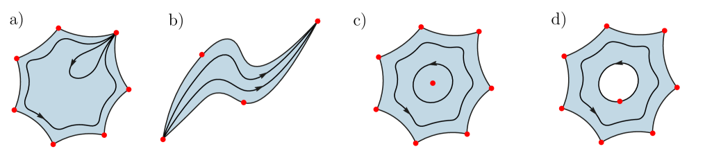
Figure 1: Real phase portraits of canonical regions of singular complex analytic vector fields ${\mathbb{X}}$, in their boundaries, pieces of trajectories and singular points (in red) appear.

Definition 2.

Let ${\mathbb{X}}$ be a singular complex analytic vector field on $({\mathbb{R}}\backslash\mathfrak{P}),J)$, the separatrix skeleton $\Gamma({\mathbb{X}})=\{z_{\vartheta}(\tau)\}$ of ${\mathbb{X}}$ is the union of its ${\mathbb{R}}$–incomplete trajectories.

Example 2.

A pole of order $k$. Let ${\mathbb{X}}$ be singular complex vector field on ${\widehat{\mathbb{C}}}$, having a pole of order $k\geq 1$, the diagram from Equation (19) is

The canonical decomposition of ${\mathbb{X}}$ is

${\widehat{\mathbb{C}}}\backslash\Gamma({\mathbb{X}})=\bigcup_{\alpha=1}^{2k+2}\big{(}{{\mathbb{H}}}^{2},\frac{\partial}{\partial z}\big{)}_{\alpha},$

having complete separatrix skeleton

$\Gamma({\mathbb{X}})=\left\{{\mathfrak{Im}\left(z^{k}\right)}=0\right\}\cup\left\{\infty\right\}\subset{\widehat{\mathbb{C}}}.$

Looking at $\infty,0\in{\widehat{\mathbb{C}}}$, the germs of ${\mathbb{X}}$ and admissible words are

$\big{(}({\mathbb{C}}_{z},0),\frac{1}{z^{k}}\frac{\partial}{\partial w}\big{)}\longleftrightarrow\underbrace{H\cdots H}_{2k+2},\ \ \ \big{(}({\mathbb{C}}_{w},0),w^{k-2}\frac{\partial}{\partial w}\big{)}\longleftrightarrow\underbrace{E\cdots E}_{2(k-2)},$ for $k\geq 3.$

Here $H$, $E$ means the hyperbolic, elliptic angular sectors of ${\mathfrak{Re}\left({\mathbb{X}}\right)}$, see Table 1 and Figure 4.a–b.

Example 3.

Consider the complex rational vector field as follows

${\mathbb{X}}(z)=\frac{z}{z^{4}-1}\frac{\partial}{\partial z}$,    $X(x,y)\doteq\rho(x,y){\mathfrak{Re}\left(\frac{z}{z^{4}-1}\frac{\partial}{\partial z}\right)}$,

for suitable $\rho$, the last is $C^{\infty}$ on ${\mathbb{R}}^{2}$. Using Figure 2.a, we note that ${\mathbb{C}}\backslash\Gamma({\mathbb{X}})$ is a union de eight strips and eight half planes.

Example 4.

The complex exponential vector field on ${\widehat{\mathbb{C}}}$. The diagram is

The vector field $X={\mathfrak{Re}\left({\mathbb{X}}\right)}$ have an infinite number of horizontal Reeb’s components on ${\mathbb{C}}$, Figure 2.c. The decomposition in canonical regions is

${\widehat{\mathbb{C}}}\backslash\Gamma({\mathbb{X}})=\bigcup_{\alpha=-\infty}^{\infty}\big{(}{\mathbb{H}}^{2},\frac{\partial}{\partial z}\big{)}_{\alpha},$

having separatrix skeleton

$\Gamma({\mathbb{X}})=\{{\mathfrak{Im}\left(z\right)}=k\pi\ |\ k\in{\mathbb{Z}}\}\cup\{\infty\}.$

Looking ${{\mathbb{X}}}$ at the point $\infty\in{\widehat{\mathbb{C}}}$, the germ and admissible word are

$\big{(}({\mathbb{C}}_{w},0),-w^{2}{\text{\myfont e}}^{-w}\frac{\partial}{\partial w}\big{)}\longleftrightarrow\mathscr{E}\mathscr{E}.$

Here $\mathscr{E}$ means the entire sector of ${\mathfrak{Re}\left({\mathbb{X}}\right)}$, see Equation (22) and Figure 4.d-e, the entire sectors come from ${\mathbb{X}}$ on $\{z\ |\ {\mathfrak{Im}\left(z\right)}>0\}$ and $\{z\ |\ {\mathfrak{Im}\left(z\right)}<0\}$.

Example 5.

An infinite number of isochronous centers. Recalling that, a simple zero with pure imaginary linear part determines an isochronous center, we consider

see Figure 3.b. The canonical decomposition is

${\widehat{\mathbb{C}}}\backslash\Gamma({\mathbb{X}})=\bigcup_{\varsigma=1}^{\infty}\big{(}\Delta_{1},\pm iz\frac{\partial}{\partial z}\big{)}_{\varsigma},$

having an infinite number of half cylinders (isochronous centers).

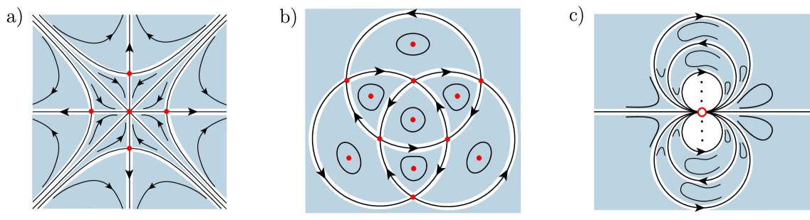
Figure 2: Decomposition in canonical regions without accumulation of singular points (in red) of ${\mathbb{X}}$ at $\infty\in{\widehat{\mathbb{C}}}_{z}$. (a) and (b) are rational vector fields, (c) is the complex exponential vector field (the small red circle denotes $\infty$).

5 Proof of Theorem 2

Proof assertion $(1)$ in Theorem 2. The main technical result for the proof is the following.

Lemma 1 ([15] p. 57, [12], [11]; Isometric glueing).

Let $(\overline{N}_{1},{\mathbb{X}}_{1})$, $(\overline{N}_{2},{\mathbb{X}}_{2})$ be two canonical regions and let $z_{1}(\tau)\subset\partial\overline{N}_{1}$, $z_{2}(\tau)\subset\partial\overline{N}_{2}$ be segments in trajectories of ${\mathfrak{Re}\left({\mathbb{X}}_{1}\right)}$ and ${\mathfrak{Re}\left({\mathbb{X}}_{2}\right)}$, having the same length. The isometric glueing of them along these geodesic boundary preserving the orientation of ${\mathfrak{Re}\left({\mathbb{X}}_{1}\right)}$ and ${\mathfrak{Re}\left({\mathbb{X}}_{2}\right)}$, is well defined, and provides a new flat surface (a Riemann surface structure) on $\overline{N}_{1}\cup\overline{N}_{2}$ arising from a new complex analytic vector field ${\mathbb{X}}$. $\Box$

By hypothesis $M$, is obtained by the paste of closed canonical regions

$$\left(\overline{\mathbb{H}}^{2},\frac{\partial}{\partial z}\right),\ \Big{(}\{0\leq{\mathfrak{Im}\left(z\right)}\leq h\},\frac{\partial}{\partial z}\Big{)},\ \left(\overline{\Delta}_{1},\frac{-2\pi iz}{r}\frac{\partial}{\partial z}\right),\ \left(\overline{\Delta}_{R}\backslash\Delta_{1},\frac{-2\pi iz}{r}\frac{\partial}{\partial z}\right),$$

$h,\,r\in{\mathbb{R}}^{*}$. Here the paste uses isometries that preserve the orientation of the real trajectories in their boundaries. The assertion follows from the Corollary 1.

Proof assertion (2) in Theorem 2. By hypothesis, the incomplete trajectories of ${\mathfrak{Re}\left({\mathbb{X}}\right)}$ are locally finite in $(M,J)$. Then, we remove the separatrix skeleton, thus $M\backslash\Gamma({\mathbb{X}})$ is an finite or infinite union of open sets invariant under the flow of ${\mathfrak{Re}\left({\mathbb{X}}\right)}$. It is well known that interior of the open sets are necessarily as in Definition 1. Thus, the Riemann surface $(M,J)$ has a decomposition

$$\begin{array}[]{r}M=\bigcup_{{\tt a}}\left(\overline{\mathbb{H}}^{2},\frac{\partial}{\partial z}\right)\bigcup_{{\tt b}}\left(\{0\leq{\mathfrak{Im}\left(z\right)}\leq h_{\tt b}\},\frac{\partial}{\partial z}\right)\bigcup_{{\tt c}}\left(\overline{\Delta}_{1},\frac{2\pi iz}{r_{\tt c}}\frac{\partial}{\partial z}\right)\bigcup_{\tt d}\left(\overline{\Delta}_{R_{\tt d}}\backslash\Delta_{1},\frac{2\pi iz}{r_{\tt d}}\frac{\partial}{\partial z}\right).\end{array}$$ (21)

The Theorem 2 is done.

Example 6.

Singular complex analytic vector fields having an infinite decomposition in canonical regions. In Figure 3 drawing (a) is the complex exponential, (b) is $isin(z)\frac{\partial}{\partial z}$. The (c)–(f) use Theorem 2; they illustrate accumulation of poles and zeros to an essential singularity at $\infty$.

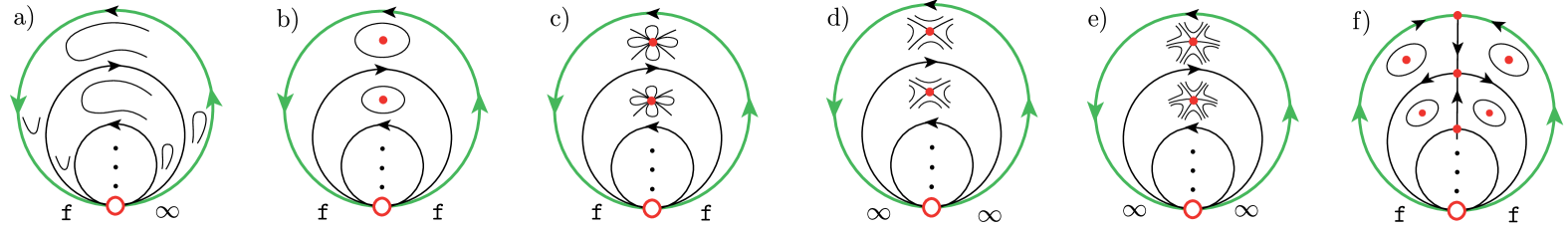
Figure 3: Singular complex analytic vector fields ${\mathbb{X}}$ on a half plane, with an infinite number of canonical pieces, accumulation of singular points (in red) and infinite number of real incomplete trajectories of ${\mathfrak{Re}\left({\mathbb{X}}\right)}$ at $\infty\in{\widehat{\mathbb{C}}}_{z}$.

Some results on the set of incomplete trajectories $\Gamma({\mathbb{X}})$ are in order.

The local analytic normal forms for poles and zeros of meromorphic complex analytic vector fields, Table 1, is well known, here in the right column $H,\,E,\,P$ means topological hyperbolic, elliptic and parabolic topological sectors for ${\mathfrak{Re}\left(X\right)}$.

Table 1: Local analytic normal forms for poles and zeros of ${\mathbb{X}}$.

normal form	analytic invariants	flat metrics	$\Psi(z)$	top. invariants
of ${\mathbb{X}}$	order & residue	$g_{\mathbb{X}}$		words
$\frac{\partial}{\partial z}$	$\hskip 22.76228pt0\hskip 22.76228pt0$	cone angle $2\pi$	$z$	$\underbrace{H\cdots H}_{2}$
$\frac{1}{z^{k}}\frac{\partial}{\partial z}$	$-k\leq-1\hskip 17.07182pt0$	cone angle $(2k+2)\pi$	$\frac{z^{k+1}}{k+1}$	$\underbrace{H\cdots H}_{2k+2}$
$\lambda z\frac{\partial}{\partial z}$	$s=1\ \ \ \ \ \lambda\in i{\mathbb{R}}^{*}$	$\mathbb{S}^{1}_{1\pi|\lambda|}\times(0,\infty)$	$\lambda log(z)$	$C$
$\lambda z\frac{\partial}{\partial z}$	$s=1\ \ \ \ \ \lambda\in{\mathbb{C}}\backslash{\mathbb{R}}$	$\mathbb{S}^{1}_{1\pi|\lambda|}\times(0,\infty)$	$\lambda log(z)$	$P$
$\frac{z^{s}}{1-\lambda z^{s-1}}\frac{\partial}{\partial z}$	$2\leq s\ \ \ \ \ \lambda\in{\mathbb{R}}$	$(2s-2)\ \hbox{copies}\ (\overline{{\mathbb{H}}}^{2},\infty)$	$\frac{1}{(1-s)z^{s-1}}+\lambda log(z)$	$\underbrace{E\cdots E}_{2s-2}$
		$(2s-2)\ \hbox{copies}\ (\overline{{\mathbb{H}}}^{2},\infty)$
$\frac{z^{s}}{1-\lambda z^{s-1}}\frac{\partial}{\partial z}$	$2\leq s\ \ \ \ \ \lambda\in{\mathbb{C}}\backslash{\mathbb{R}}$	and a strip	$\frac{1}{(1-s)z^{s-1}}+\lambda log(z)$	$\underbrace{E\cdots E}_{2s-2}P$

Corollary 5.

Let ${\mathbb{X}}$ a singular complex analytic vector field on a simply connected Riemann surface $(M,J)$ as above. The following assertions are equivalent.

1) $(M,J)={\mathbb{C}}$ or ${\widehat{\mathbb{C}}}$ and in any case ${\mathbb{X}}$ is (the restriction of) a rational vector field on ${\widehat{\mathbb{C}}}$.

2) For each rotated vector field ${\text{\myfont e}}^{i\theta}{\mathbb{X}}$, its set of incomplete real trajectories $\Gamma({\text{\myfont e}}^{i\theta}{\mathbb{X}})$ is finite.

3) The decomposition of ${\mathbb{X}}$ on $(M,J)$ has a finite number of canonical regions and no finite trajectory gap, i.e. a segment of geodesic in the boundary of a canonical region that is not identified in $(M,J)$.

Proof.

Assume Table.1 and let ${\mathbb{X}}$ be a complex rational vector field on ${\widehat{\mathbb{C}}}_{z}$. The incomplete trajectories are the separatrices at poles, hence they are finite number for each rotated vector field ${\mathfrak{Re}\left({\text{\myfont e}}^{i\theta}{\mathbb{X}}\right)}$, we perform the assertion (2). If we assume (2), then the separatrices are a finite number, and the decomposition in canonical pieces is finite. Moreover, the poles and zeros are conformal punctures of the complex structure $(M,J)$, this is no gap trajectory can appear; see Corollary 1 and its proof in $\mathchar 632\relax$ 6. We leave the converse assertions for the reader. ∎

Moreover, a local version of Theorem 2 provides new non isolated singularities of complex analytic vector fields, we give a very brief description. The topological hyperbolic, elliptic and parabolic sectors for real vector fields of vector fields germs are illustrated in Figure 4.a–c. Moreover they are analytic germs and suitable flat metrics as follows.

The germs of singular complex analytic vector fields $\big{(}({\mathbb{C}},q),\mathbb{X}\big{)}$ on angular sectors are as follows:

$$\begin{array}[]{lll}\hbox{a \emph{isochronous center at } }q=0&&C=\left(({\mathbb{C}},0),\ \frac{iz}{r}\frac{\partial}{\partial z}\right),\ r\in{\mathbb{R}}^{+},\\ \hbox{a \emph{hyperbolic sector at } }q=0&&H=\left(\big{(}\overline{{\mathbb{H}}}^{2},0\big{)},\ \frac{\partial}{\partial z}\right),\\ \hbox{an \emph{elliptic sector at } }q=\infty&&E=\left(\big{(}\overline{{\mathbb{H}}}^{2},\ \infty\big{)},\frac{\partial}{\partial z}\right),\\ \hbox{a \emph{parabolic sector, at } }q=+\infty&&P=\left(\left(\{0\leq{\mathfrak{Im}\left(z\right)}\leq h\},\pm\infty\right),\ \frac{\partial}{\partial z}\right),\ h\in{\mathbb{R}}^{+},\\ \hbox{a \emph{1--class entire sector at }}q=\infty&&\mathscr{E}_{1}=\left(\big{(}\overline{{\mathbb{H}}}^{2},\infty\big{)},\ {\text{\myfont e}}^{z}\frac{\partial}{\partial z}\right).\end{array}$$ (22)

Figure 4: Hyperbolic, elliptic and parabolic sectors are sketched in (a)–(c). Entire sector in (d)–(e). Other interesting sectors in (f)–(i). The signs ${\tt f}$ and $\infty$ in the boundaries, describe the finite or infinite time of the boundary separatrix to reach at the singularity at the vertex.

In order to recombine the angular sectors in Figure 4 for perform new singularities, we consider as combinatorial information a finite cyclic word

$$\mathcal{W}=W_{1}\cdots W_{k}\ ,\ \ \ W_{\iota}\ \hbox{ in the Figure 4 alphabet}.$$ (23)

The following conditions are satisfied by $\mathcal{W}$.

Each $W_{\iota}$ can be interpreted also as a Riemannian manifold and an angular vector field germ $((\mathcal{A}_{\iota},q_{\iota}),{\mathbb{X}}_{\iota})\cong W_{\iota}$.

The geodesic boundary of $W_{\iota}$ has orientation and time to reach the singular point denoted ${\tt f}$ when is finite or $\infty$, in our figures. We consider cyclic words in the sense that

$W_{k+1}\doteq W_{1}$.

In order to perform the geometric paste of the angular sectors, we require the following additional rule; if the orientation and the time ${\tt t}$ or $\infty$ coincide
then the two trajectories can be pasted together. We have a new version of the result in [3] p. 167:

Corollary 6.

1. The paste as above of a finite number of angular sectors $\mathcal{W}$ determines a germ of singular complex analytic vector field $\big{(}({\mathbb{C}},0),{\mathbb{X}}\big{)}$ with singularity at $0$.

2. The singularity $0$ is a pole or zero of ${\mathbb{X}}$ if and only if a center, a finite number of hyperbolic, elliptic and/or parabolic sectors appear at $0$, recall Table 1. $\Box$

In the above, the vertex of the angular sectors is a conformal puncture, hence the singularity is a zero, a pole or an essential singularity of ${\mathbb{X}}$. The alphabet in Figure 4 is far from begin complete, however it shows the wealth of the theory.

6 On the conformal type problem

Definition 3.

Let $J$ be complex structure on $M\subset{\mathbb{R}}^{2}$ such that $X={\mathfrak{Re}\left({\mathbb{X}}\right)}$ is the real part of a complex analytic vector field ${\mathbb{X}}$ on $(M,J)$. ${\mathbb{X}}$ has a finite trajectory gap at the ideal boundary $\infty$ if there exists a local (holomorphic) flow box

$$\Psi:(U\subset M,J)\longrightarrow{\mathbb{C}},\ \text{such that}\ \lim_{U\ni(x,y)\to\infty}\psi(x,y)=\beta\subset{\mathbb{C}},$$

where $(x,y)\to\infty$ means that $(x,y)$ tends to the ideal boundary of $M$, and $\beta$ is a simple path in ${\mathbb{C}}$ different from a point, see Figure 5.

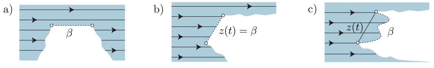
Figure 5: A finite trajectory gap means that the ideal boundary of the metric $g_{\mathbb{X}}$ (under a local flow box) is $\beta$.

Proof of Corollary 3. Using the vector fields, we provide elementary arguments, compare with [2] Ch. 10. Let $X$ be a vector field on a simply connected $(M,J)$ having a finite trajectory gap.

Case 1. The path $\beta\in{\mathbb{C}}$, gap is a segment of trajectory of ${\mathbb{X}}$. i.e. there exists in $\big{(}({\mathbb{R}}^{2},J),X\big{)}$ a holomorphic local flow box $\Psi:U\subset{\mathbb{R}}^{2}\to(0,\epsilon)\times(0,i\epsilon)\subset{\mathbb{C}}$ such that $\Psi^{-1}(x+i0)$ is in the ideal boundary of ${\mathbb{R}}^{2}$, Figure 5.a.

We proceed by contradiction, let $\pi:{\mathbb{C}}\to({\mathbb{R}}^{2},J)$ the uniformization of the adapted complex structure to $X$. The map $\pi^{-1}$ sends the ideal boundary of ${\mathbb{R}}^{2}$ to $\infty\in{\widehat{\mathbb{C}}}$.

Then the composition $(\frac{1}{z})\circ\pi\circ\psi:(0,\epsilon)\times(0,i\epsilon)\to{\mathbb{C}}$ is a biholomorphic map, continuous and real valued in $\{x+i0\}$. Using the reflection principle, we can extend $(\frac{1}{z})\circ\pi\circ\psi$ to a holomorphic $\phi:(0,\epsilon)\times(-i\epsilon,i\epsilon)\to{\mathbb{C}}$, defining $\phi(x+iy)\doteq\overline{(\frac{1}{z})\circ\pi\circ\psi}(x-iy)$ for $x+iy$ in the lower rectangle, $(\overline{\ \ })$ is the complex conjugation. As a result $\phi$ is a local biholomorphism in the upper and low open rectangles and $\phi(x+i0)\equiv 0$, that is a contradiction.

Case 2. The path $\beta\in{\mathbb{C}}$ is a straight line segment. There exists a rotation ${\text{\myfont e}}^{i\theta}$, such that $\psi^{-1}(\beta)$ coincides with a trajectory of ${\text{\myfont e}}^{i\theta}X$, see Figure 5.b. Hence we can apply the above argument.

Case 3. The path $\beta$ has arbitrary shape in ${\mathbb{C}}$. Assume by a moment that there is a trajectory $z(t)$ of ${\text{\myfont e}}^{i\theta}X$ that determine a secant of $\beta$, see Figure 5.c. By case 2 the conformal structure on the surface $(M^{\prime}\subset{\mathbb{R}}^{2},J)$ bounded by $z(t)$ has conformal hole. The region $(U^{\prime}J)$ bounded by $z(t)$ and $\beta$ is biholomorphic to the Poincaré disk $\Delta$. If we consider the paste of $(M^{\prime}\cup\Delta,J)$ obviously also has a conformal hole.

The finite trajectory gap concept can be used for vector field germs $X={\mathfrak{Re}\left({\mathbb{X}}\right)}$ on $(({\mathbb{R}}^{2}\backslash\{\overline{0}\},\overline{0}),J)$, where the ideal boundary to be consider is $\overline{0}$. In this case, the existence of a finite trajectory gap, means that $0$ is a conformal hole of $(({\mathbb{R}}^{2}\backslash\{\overline{0}\},\overline{0}),J)$. $\Box$

7 Complex structures around isolated singularities

Recall assertion (1) in Corollary 1. Let $H\subset{\mathbb{R}}^{2}$ be a topological hyperbolic sector of $X$ above, having as boundary a vertex at $p\in\mathfrak{P}\cup\{\infty\}$ and two separatrix trajectories $\zeta_{1}$, $\zeta_{2}\subset\partial H\cap{\mathbb{R}}^{2}$, with $\alpha$ and $\omega$–limits at $p$ (or viceversa). Let $q_{j}\in\zeta_{j}$ $j=1,2$, be two nonsingular points of $X$ and consider $C^{\infty}$ embedded transversals to $X$,

$\sigma_{j}:[0,\epsilon)\longrightarrow\Sigma_{j}\subset H,\ \ \sigma_{j}(0)=q_{j}$

as manifolds with boundary. There exists a holonomy map of $X$

$$hol:(\Sigma_{1},q_{1})\longrightarrow(\Sigma_{2},q_{2}),\ \ (x,y)\longmapsto\phi_{\tau(x,y)}(x,y),\\$$ (24)

here $\phi_{\tau}(\ ,\ )$ is the flow of $X$ and $\tau=\tau(x,y)$ is a suitable time function on $\Sigma_{1}\backslash\{q_{1}\}$. The map $hol$ is a $C^{\infty}$ diffeomorphism in the interior points of $\Sigma_{1},\Sigma_{2}$.

Definition 4.

The holonomy of an hyperbolic sector $H$ is a $C^{\infty}$ diffeomorphism when the germ $hol:(\Sigma_{1},q_{1})\longrightarrow(\Sigma_{2},q_{2})$ is a $C^{\infty}$ diffeomorphism of manifolds with boundary, see Figure 6.

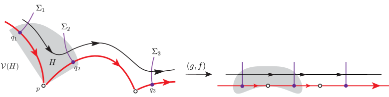
Figure 6: The composition of holonomy maps, must be a $C^{\infty}$ diffeomorphism between transversals including their boundary points $q_{1},q_{2}\in\Gamma(X)$ inside of separatrices arriving or leaving $p\in\mathfrak{P}\cup\{\infty\}$, according to Definition 4.

As far as we known, Definition 4 is due to W. Kaplan [8] p. 224, it was called evenly spread, in J. L. Weiner [16] p. 201 is $\infty$–normal, and also appeared in H. Zoladek [17].

Corollary 1 is now clear, we provide some interesting examples related to real vector fields.

Example 7.

A prototype. The holonomy of a linear hyperbolic sector $H$ of

$X(x,y)=\lambda_{1}x\frac{\partial}{\partial x}+\lambda_{2}y\frac{\partial}{\partial y}$, $\lambda_{1}\lambda_{2}<0$,

is a $C^{\infty}$ diffeomorphism if and only if $\lambda_{1}=-\lambda_{2}$. Moreover, in this case the first integral is $f(x,y)=xy$ and the infinitesimal symmetry is

$Y(x,y)=\frac{1}{x^{2}+y^{2}}\big{(}y\frac{\partial}{\partial x}+x\frac{\partial}{\partial y}\big{)}$.

Example 8.

A holonomy map which is not a $C^{\infty}$ diffeomorphism, M.–P. Muller [13]. Let us consider

$X(x,y)=-x^{4}\frac{\partial}{\partial x}+(x^{3}y+2xy+2)\frac{\partial}{\partial y}\ \in C^{\infty}({\mathbb{R}}^{2}).$

The holonomy of the hyperbolic sector $H$, with vertex in $\infty\in\SS^{2}$ which is bounded by the separatrices $\zeta_{1}=\{(0,\tau)\ |\ \tau<0\}$, $\zeta_{2}=\{(\tau,-1/\tau)\ |\ 0<\tau<1\ \},$ of the vector field $X$ is not a diffeomorphism. For this computation Muller used the Liouvillian first integral $f(x,y)=(xy+1){\text{\myfont e}}^{-1/x^{2}}$. The infinitesimal symmetry $Y=\nabla{f}/\|\nabla{f}\|^{2}$ is not $C^{1}$ at $\zeta_{1}$.

Example 9.

The cusp; a removable singularity. The Hamiltonian vector field

$X_{f}(x,y)=my^{m-1}\frac{\partial}{\partial x}+nx^{n-1}\frac{\partial}{\partial y}\ \ \ \hbox{on }\mathbb{R}^{2}$

of the function $f(x,y)=x^{n}-y^{m}$, where $n,m\geq 2$ and $(n,m)=1$, have at $\overline{0}$ a 2–saddle. The union of the separatrices is the singular cusp $\{x^{n}-y^{n}=0\}$ at $\overline{0}$. If $n$ is even $\rho(x,y)={\text{\myfont e}}^{-x}/(mx^{m-1}+ny^{n})$ is a scaling factor for $X_{f}$ and there exists a second vector field

$Y_{g}(x,y)=-{\text{\myfont e}}^{x}\frac{\partial}{\partial x}+y{\text{\myfont e}}^{x}\frac{\partial}{\partial y}$

linearly independent with $X_{f}$, such that $[\rho X_{f},\rho Y_{g}]\equiv 0$ on $\mathbb{R}^{2}$. The Proposition 2 applies and there exists a global flow box

$\Psi(x,y)=(y{\text{\myfont e}}^{x},x^{m}-y^{n})$

for $\rho X_{f}$ on ${\mathbb{R}}^{2}\backslash\{0\}$. Analogously, if $n$ is odd, there exist a scaling factor $\rho(x,y)={\text{\myfont e}}^{-y}/(mx^{m}+ny^{n-1})$ and a global flow box $\Psi(x,y)=(x{\text{\myfont e}}^{y},x^{m}-y^{n})$ for $\rho X_{f}$.

Example 10.

Topological saddles with zero linear part. The vector field

$X(x,y)=x^{3}\frac{\partial}{\partial x}-y^{3}\frac{\partial}{\partial y}$

determines a topological saddle on $({\mathbb{R}}^{2},\overline{0})$. Its foliation $\mathcal{F}(X)$ is symmetric respect to reflection on both axes, hence the holonomy of each hyperbolic sector is a $C^{\infty}$ diffeomorphism on a punctured neighbourhood of $\overline{0}$. There exists a single valued local diffeomorphism $\Xi:({\mathbb{R}}^{2}\backslash\{\overline{0}\},\overline{0})\longrightarrow({\mathbb{R}}^{2}-\{\overline{0}\},\overline{0})$ such that

$$\Xi_{*}(\rho_{2}(x,y)X(x,y))=x\frac{\partial}{\partial x}-y\frac{\partial}{\partial y},$$

for suitable $\rho_{2}$. The flow box around $\overline{0}$ exists, and is $\Xi\circ\Psi$.

Example 11.

The saddle node. Let $X\in\mathfrak{X}^{\infty}({\mathbb{R}}^{2},\overline{0})$ be a saddle node

$X(x,y)=x^{2}\frac{\partial}{\partial x}-\lambda y\frac{\partial}{\partial y},\ \ \ \lambda\in{\mathbb{R}}^{+}$.

The function ${\tt f}(x,y)=e^{\lambda/x}/y$ is a Liouvillian first integral. The holomomy of the hyperbolic sectors is not a $C^{\infty}$ diffeomorphism. Hence, even in the punctured germ domain $({\mathbb{R}}^{2}\backslash\{\overline{0}\},\overline{0})$ does not exist an adapted complex structure making $X$ the real part of a singular complex analytical vector field. Using a reparametrization

$\rho(x,y)X(x,y)=\frac{1}{(x^{2}+y^{2})}\left(x^{2}\frac{\partial}{\partial x}-\lambda y\frac{\partial}{\partial y}\right),$

the trajectories of $\rho X$ arrives $\overline{0}$ at finite time. Moreover, if we remove the origin and the positive real $x$ axis; there exists an adapted complex structure making to $\rho X$ the real part of a holomorphic vector field on $({\mathbb{R}}^{2}\backslash\{(x,0)\ |\ x\geq 0\},J)$, see Figure 7. In fact, we consider an embedded transversal to $\rho X$,

$\sigma:(-\epsilon,\epsilon)\longrightarrow\Sigma_{1}\subset{\mathbb{R}}^{2}\backslash\{(x,y)\ |\ (x,0),x\geq 0\}$.

The vector field $Y$ tangent to $\Sigma_{1}$ is transversal to $\rho X$. We extend this transversal data over the whole domain ${\mathbb{R}}^{2}\backslash\{(x,0)\ |\ 0\leq x\}$ using the flow of $\rho X$; this produces a vector field $Y$, such that $[\rho X,Y]=0$. Figure 7 shows the target of the global flow box $\Psi=(g,f)$ and the shape of the associated flat surface. When we identify the two right boundaries of the regions $H$, the origin 0 becomes a finite trajectory gap (a conformal hole) of the resulting $({\mathbb{R}}^{2}\backslash\{0\},J)$ where $J(\rho X)=Y$ and $J(Y)=-\rho X$.

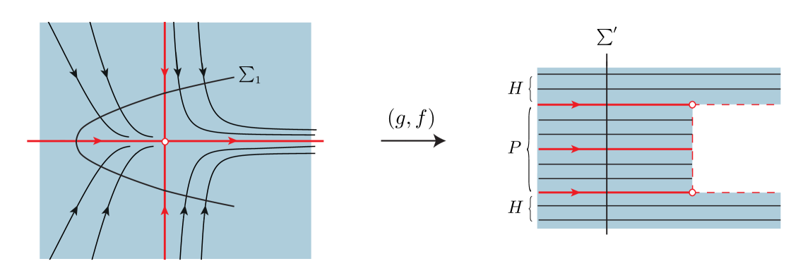
Figure 7: The saddle node $X(x,y)=x^{2}\frac{\partial}{\partial x}-\lambda y\frac{\partial}{\partial y}$ determines the word $HPH$ at $\overline{0}$; a global flow box exists on the plane minus a ray $\{(x,0)\ |\ 0\leq x\}$, here $\rho X$ becomes the real part of a holomorphic vector field.

The converse of Corollary 1 is the goal of a future work.

References

[1]
L. V. Ahlfors,
Complex Analysis
Third Ed.
(McGraw–Hill, Tokyo, 1979).
[2]
L. V. Ahlfors,
Conformal Invariants: Topics in Geometric Function Theory
(McGraw–Hill, U.S.A. 1973).
[3]
A. Alvarez–Parrilla and J. Muciño–Raymundo,
‘‘Complex analytic vector fields with essential singularities I,’’
Conf. Geom. Dyn. 21, 126–224
(2017).
[4]
V. I. Arnold,
‘‘Wave front evolution an equivariant Morse lemma,’’
Comm. Pure Appl. Math.
29, 557–582 (1976).
[5]
W. M. Boothby,
‘‘The topology of level curves of harmonic functions with critical points,’’
Amer. J. Math. 73, 3, 512–53 (1951).
[6]
R. Bott,
‘‘Marston Morse and his mathematical works,’’
Bull. Amer. Math. Soc.
3, 3, 907–950 (1980).
[7]
N. H. Ibragimov,
Elementary Lie Group Analysis and Ordinary Differential Equations,
(John Wiley & Sons, Chichester, 1999).
[8]
W. Kaplan,
‘‘On partial differential equations of first order,’’
in Topics in Analysis, Jyväskylä 1970
(Lecture notes in Math. 419, Springer, Berlin, 1974),
pp. 221–231.
[9]
J. A. Jenkins,
Univalent Functions and Conformal Mapping,
(Springer–Verlag, Berlin, 1958).
[10]
S. Kobayashi and K. Nomizu,
Foundations of Differential Geometry,
Vol. II.
(John Wiley & Sons, New York, 1969).
[11]
J. Muciño–Raymundo,
‘‘Complex structures adapted to smooth vector fields,’’
Math. Annalen, 322, 229–265 (2003).
[12]
J. Muciño–Raymundo and C. Valero–Valdéz,
‘‘Bifurcations of meromorphic vector fields on the Riemann sphere,’’
Ergod. Th. & Dynam. Sys. 15, 1211-1222 (1995).
[13]
M. P. Muller,
‘‘An analytic foliations of the plane without weak first integrals of
class ,’’
Boletín de la Soc. Mat. Mex., (2) 21, 1, 1–5 (1976).
[14]
A. A. Du Plessis and Ch. T. C. Wall,
Discriminants and vector fields, in
Singularities, Progress in Mathematics, Vol. 162,
Birkhäuser, 119–140 (1998).
[15]
K. Strebel,
Quadratic Differentials
(Springer–Verlag, Berlin, New York, 1984).
[16]
J. L. Weiner,
‘‘First integrals for a direction field on a simply connected plane domain,’’
Pacific J. Math. 132, 1, 195–208 (1988).
[17]
H. Zoladek,
‘‘On the first integrals for polynomial differential equations on the line,’’
Studia Math., 107, 2, 205–211 (1993).