Parameter Convex Neural Networks

Abstract

Deep learning utilizing deep neural networks (DNNs) has achieved a lot of success recently in many important areas such as computer vision, natural language processing, and recommendation systems. The lack of convexity for DNNs has been seen as a major disadvantage of many optimization methods, such as stochastic gradient descent, which greatly reduces the genelization of neural network applications. We realize that the convexity make sense in the neural network and propose the exponential multilayer neural network (EMLP), a class of parameter convex neural network (PCNN) which is convex with regard to the parameters of the neural network under some conditions that can be realized. Besides, we propose the convexity metric for the two-layer EGCN and test the accuracy when the convexity metric changes. For late experiments, we use the same architecture to make the exponential graph convolutional network (EGCN) and do the experiment on the graph classificaion dataset in which our model EGCN performs better than the graph convolutional network (GCN) and the graph attention network (GAT).

1 Introduction

Deep neural networks have received flood of attention on account of unbeatable success in many fields, such as computer vision Krizhevsky et al. (2012), natural language processing Hinton et al. (2012) and recommendation system Guo et al. (2017). Despite good performance by some first-order gradient based optimization algorithms such as stochastic gradient descent (SGD), it is still theoretically incomprehensible that how and why such algorithms can train deep neural networks (DNNs) successfully. Optimization algorithms such as stochastic gradient descent (SGD) cause many problems that the optimization algorithms are not sure to converge to a stable point and the global minimum points are hard to get. However, even though the optimization algorithms can converge to a stable point, it’s still hard to decide whether the stable point is a global minimum point even local minimum point.

The global minimum point is hard to solve in nonconvex problems and deep learing is just a representative nonconvex problem that the object function is very complicated and nonconvex. The loss function has many critical points to make the problem more difficult and there are many works about how a critical point can be a global minimum point. For deep linear neural networks, a sufficient and necessary condition that the critical point of the objective function is the global minimum point is proposed by Yun et al. (2017). Besides, Haeffele and Vidal (2017) also shows that the global minimum point can just be the local minimum point under sufficient conditions, and when they make the network output and regularization to be positive homogeneous functions of network parameters with the regularization design used to control the size of the network, the local descent method can achieve the global minimum under any initialization conditions. Boob and Lan (2017) shows that for a broad class of differentiable activation functions, the first-order optimal solution can be global minimum point as long as the hidden layer is non-singular. Nguyen and Hein (2017) shows that (almost) so, in fact almost all local minimun points are global optimal minimun points, and that the fully connected network with square losses and the analytic activation function assume that the number of hidden quantitative units in a layer of networks is greater than the training fraction, and that the network structure of this layer is pyramidal. The most popular algorithm for deep learning optimization is stochastic gradient descent and there are lots of works about the global minimum point when utilizing SGD under different limited conditions. Li and Yuan (2017) shows that SGD converges to the global minimum point with a polynomial number of steps and is initialized with the standard deviation $O(1/d)$ when the input follows from a Gaussian distribution. Kawaguchi and Huang (2019) proves theoretically that gradient descent method can find the global minimum point of non-convex optimization for all layers of nonlinear deep neural networks of various sizes. Unlike gradient descent and quasi-Newton methods, other works put forward some different algorithms that may get the solution which is the global minimum point. Dauphin et al. (2014) proposes a new second-order optimization method, the saddle-free Newton method, which can avoid high dimensional saddle points quickly. Also, Wu et al. (2019) proposes an adaptive gradient algorithm and proves that for two-layer over-parameterized neural networks, if the width of the net is large enough (polynomially), the algorithm converges to the global minimum point in polynomial time. Besides, some unique works get the global minimum point in unexpected way. Gradient descent method achieves zero loss in the train dataset in polynomial time for a deep overparameterized neural network Du et al. (2019) with residual connections (ResNet). Sun et al. (2020) points out that there may be suboptimal local minimum points in generalized neural networks under certain hypothetical conditions, and discuss some strict results of geometric properties of generalized neural networks, such as no bad basin, and elimination of suboptimal local minimum points and reduction of paths to infinity.

Convergence is also a popular hotspot for training the deep neural networks. When the initialization is correct in the multiparticle limit, the gradient flow, though non-convex, converges to a global minimum point Chizat and Bach (2018). For shallow neural networks with $m$ hidden nodes activated by ReLU and training data, Du et al. (2018) proves that as long as $m$ is large enough and there are no two parallel inputs, the randomly initialized gradient descent function converges to the global optimal minimum solution at a linear convergence rate. Wang and others (2018) proves that the convergence rate of deep neural network approximations is exponential for low dimensional analytic functions. Allen-Zhu et al. (2019) shows that simple algorithms, such as stochastic gradient descent (SGD), can find global minimum point on training datasets in polynomial time, provided that the input does not degenerate and the network is over-parameterized. Sun et al. (2020) briefly discusses some convergence results and their relationship with the neural network landscape results. Zhou et al. (2021) shows that as long as the loss is less than a threshold value, in an over-parameterized double-layer neural network, all the student neurons will converge to one of the teacher neurons and the loss will approach zero.

In this paper, we don’t analyse the global minimum point and convergence for deep neural networks. Instead, we remould the deep neural networks and propose the Parameter Convex Neural Network (PCNN) which is convex to the parameters. We first transform the multilayer neural network (MLP) to exponential multilayer neural network (EMLP) and use the same technique to make the exponential graph convolutional network (EGCN) converted from the GCN. As far as we know, this is the fisrt time that the convex neural network to parameters but not input is proposed. Besides, we experiment our model on classification assignment and get excellent results.

2 Models

2.1 Notations, Definitions and Theorems

Respectively, we denote the matrices, vectors and scalars as uppercase bold letters (such as $\boldsymbol{A}$), lowercase bold letters (such as $\boldsymbol{a}$) and lowercase letters (such as $a$). To denote a vector or matrix of zeros, we use $\boldsymbol{0}$, where the size is acquired from the context. In addition, We list some notations for the future use.
$\boldsymbol{A}\odot\boldsymbol{B}$  Hadamard product
$\boldsymbol{A}\otimes\boldsymbol{B}$  Kronecker product
$\boldsymbol{A}^{n}$  $n$ times Hadamard product of $A$
diag($\boldsymbol{x}$)  turn a vector into a diagonal matrix
$vec(\boldsymbol{W})$  vec operator transforms a matrix into a vector by stacking the columns of the matrix one underneath the other
$a^{\boldsymbol{W}}$  exponential operator transforms a matrix into another matrix with the same size and transform every element $\boldsymbol{W}_{ij}$ into $a^{\boldsymbol{W}_{ij}}$
$log_{a}(\boldsymbol{W})$  logarithm operator transforms a matrix into another matrix with the same size and transform every element $\boldsymbol{W}_{ij}$ into $log_{a}(\boldsymbol{W}_{ij})$
$\boldsymbol{x}>(\geq)\boldsymbol{0}$  every element $\boldsymbol{x}_{i}>(\geq)0$
$\boldsymbol{A}\succ(\succeq)0$   $\boldsymbol{A}$ is a positive (semi)definite matrix
$\boldsymbol{A}\prec(\preceq)0$   $\boldsymbol{A}$ is a negative (semi)definite matrix

To make a class of the PCNN, we first recall the second-order conditions of convex functions. We now assume that $f$ is twice differentiable, that is, its Hessian or second derivative $\bigtriangledown^{2}f$ exists at each point in dom $f$, which is open. Then $f$ is convex if and only if dom $f$ is convex and its Hessian is positive semidefinite:

$$\forall\boldsymbol{x}\in domf,\bigtriangledown^{2}f(\boldsymbol{x})\succeq 0.$$

Because the parameters of the neural network are a series of matrices, we need first to define the Hessian of functions when independent variables are matrices. If $f(\boldsymbol{X})$ is a scalar function in which $X$ is a matrix, then the Hessian can be simply defined:

$$H=f_{vec(\boldsymbol{X})(vec(\boldsymbol{X}))^{T}}$$

which can be equivalent to the Hessian of $f$ to $vec(\boldsymbol{X})$. This method is very hard to calculate, so we calculate the Hessian with another method in this paper:

$$d^{2}f=(d\,vec(\boldsymbol{X}))^{T}\boldsymbol{B}\,d\,vec(\boldsymbol{X})$$

so that

$$H=\dfrac{1}{2}(\boldsymbol{B}+\boldsymbol{B}^{T}).$$

For more information with the Hessian, you can see the book Magnus and Neudecker (2019) to learn more accurate definition of the Hessian and more methods to calculate. We now define the convex matrix funtion of matrices.

Definition 1 (convex matrix funtion).

Given a matrix function $\boldsymbol{F}(\boldsymbol{x})$ (vector function $\boldsymbol{f}(\boldsymbol{x})$ or scalar function $f(\boldsymbol{x})$) in whcih $\boldsymbol{x}$ is a scalar, vector, matrix or their conbinations, we say $\boldsymbol{F}(\boldsymbol{x})$ is (strictly) convex corresponding to $\boldsymbol{x}$ if and only if each element of $\boldsymbol{F}(\boldsymbol{x})$ is (strictly) convex corresponding to $\boldsymbol{\theta}$ which is a column vector denotation of $\boldsymbol{x}$.

This definition means that no matter what $\boldsymbol{x}$ is, we just consider the $\boldsymbol{x}$ as a column vector to judge the convex function. Then we define the PCNN and ICNN in details.

Definition 2 (PCNN,ICNN).

$\boldsymbol{F}(\boldsymbol{x},\boldsymbol{\theta})$ is a neural network, in which $\boldsymbol{x}$ is input and $\boldsymbol{\theta}$ represents parameters. We say $\boldsymbol{F}(\boldsymbol{x},\boldsymbol{\theta})$ is a Parameter Convex Neural Network (PCNN) if and only if $\boldsymbol{F}(\boldsymbol{x},\boldsymbol{\theta})$ is convex with regard to $\boldsymbol{\theta}$. Say $\boldsymbol{F}(\boldsymbol{x},\boldsymbol{\theta})$ is the Input Convex Neural Network (ICNN) if and only if $\boldsymbol{F}(\boldsymbol{x},\boldsymbol{\theta})$ is convex with regard to $\boldsymbol{x}$.

The late proof will calculate the Hessian when the argument $\boldsymbol{W}$ is a matrix. Just as the definition of the PCNN and the ICNN, we calculate the gradient and Hessian for $vec(\boldsymbol{W})$.

2.2 Multilayer Neural Network

A simple layer of the multilayer neural network (MLP) $f(\boldsymbol{W},\boldsymbol{x})$ can be defined as:

$$\boldsymbol{x}^{(n+1)}=\sigma({\boldsymbol{W}_{n}}\boldsymbol{x}^{(n)})$$ (1)

in which $\boldsymbol{W}_{n}$ is the parameters of the $n$-th layer, $\boldsymbol{x}^{(n)}$ is the $n-$th layer and $\sigma$ is the activation function with $\boldsymbol{x}^{(0)}=\boldsymbol{x}$ is the input and $\boldsymbol{W}$ is all parameters of $f$. We define the MLP $f_{n}(\boldsymbol{W},\boldsymbol{x})$ of $n$ layers as:

$$f_{n}(\boldsymbol{W},\boldsymbol{x})=\boldsymbol{x}^{(n)}={\boldsymbol{W}_{n-1}}\boldsymbol{x}^{(n-1)}$$ (2)

We just calculate the Hessian of the MLP (input and output are scalars) of two layers:

$$f(\boldsymbol{W},\boldsymbol{x})=\boldsymbol{W}_{1}^{T}\sigma(\boldsymbol{W}_{0}x).$$ (3)

in which $\boldsymbol{W}_{1}$ and $\boldsymbol{W}_{0}$ are column vectors. We just list the result of the computing without calculation details:

$$f_{\boldsymbol{W}_{1}\boldsymbol{W}_{1}} =0$$ (4)

$$f_{\boldsymbol{W}_{1}\boldsymbol{W}_{0}} =x\otimes diag(\sigma^{{}^{\prime}}(\boldsymbol{W}_{0}x))$$ (5)

$$f_{\boldsymbol{W}_{0}\boldsymbol{W}_{0}} =x^{2}diag(\sigma^{{}^{\prime\prime}}(\boldsymbol{W}_{0}x)\odot\boldsymbol{W}_{1}).$$ (6)

Then we can get the Hessian:

$$H(f)=\begin{bmatrix}f_{\boldsymbol{W}_{1}\boldsymbol{W}_{1}}&f_{\boldsymbol{W}_{1}\boldsymbol{W}_{0}}\\ f^{T}_{\boldsymbol{W}_{1}\boldsymbol{W}_{0}}&f_{\boldsymbol{W}_{0}\boldsymbol{W}_{0}}\end{bmatrix}$$ (7)

in which we just use the symbol $f_{\boldsymbol{W}\boldsymbol{W}}$ to replace $f_{vec(\boldsymbol{W})(vec(\boldsymbol{W}))^{T}}$ for simplicity. For the computing details, you can learn methods from the book Magnus and Neudecker (2019). From the Hessian, we can know that to make the Hessian positive definite, we need to transform the Hessian to make $f_{\boldsymbol{W}_{1}\boldsymbol{W}_{1}}\succeq 0$.

2.3 Exponential Multilayer Neural Network

We think a lot of methods to make $f_{\boldsymbol{W}\boldsymbol{W}}\succeq 0$, such as transforming $\boldsymbol{W}$ to $\boldsymbol{W}^{2}$ or $a^{\boldsymbol{W}}$. The model that we create is the Exponential Multilayer Neural Network (EMLP). Just as its name implies, EMLP uses exponential layer. The exponential layer is defined as:

$$\boldsymbol{x}^{(n+1)}=\sigma(a^{\boldsymbol{W}_{n}}\boldsymbol{x}^{(n)}).$$ (8)

in which $\boldsymbol{x}^{(n)}$ is the $n$-th layer of the EMLP and $\sigma$ is the activation function with the exponential hyperparameter $a$. We define the EMLP $f_{a,n}(\boldsymbol{W},\boldsymbol{x})$ of $n$ layers as:

$$f_{a,n}(\boldsymbol{W},\boldsymbol{x})=\boldsymbol{x}^{(n)}=a^{\boldsymbol{W}_{n-1}}\boldsymbol{x}^{(n-1)}$$ (9)

in which $\boldsymbol{x}^{(n-1)}$ can be get from the iteration equation 8 and $\boldsymbol{x}^{(0)}=\boldsymbol{x}$ with the exponential hyperparameter $a$. The last layer of the EMLP $f_{a}(\boldsymbol{W},\boldsymbol{x})$ is with no activation function which is natural for regression assignments. For classifiction assignments, we take softmax funcion as one part of the cross entropy function.

We first prove the convexity of a simply condition of the EMLP. All the proofs are put in supplementary material.

Theorem 1.

Let scalar $x>0$, $\sigma(x)>0$, $\sigma^{{}^{\prime}}(x)>0$, $\sigma^{{}^{\prime\prime}}(x)>0$, $a>0$ and $a\neq 1$. Let

$$f(\boldsymbol{W})=a^{\boldsymbol{W}_{2}^{T}}\sigma(a^{\boldsymbol{W}_{1}}x)$$

in which $\boldsymbol{W}_{1}$ and $\boldsymbol{W}_{2}$ are column vectors and $\boldsymbol{W}$ represents parameters $\boldsymbol{W}_{1}$ and $\boldsymbol{W}_{2}$. Then $f(\boldsymbol{W})$ is convex corresponding to $\boldsymbol{W}$ if and only if

$$\forall x>0,x\sigma^{{}^{\prime\prime}}(x)\sigma(x)+\sigma(x)\sigma^{{}^{\prime}}(x)\geq x\sigma^{{}^{\prime}2}(x).$$

Theorem 1 just presents the simplest condition of the EMLP. We will give a more general of the EMLP int the following theorems.

Theorem 2.

Suppose $\boldsymbol{x}>\boldsymbol{0}$, $\sigma(\boldsymbol{x})>\boldsymbol{0}$, $\sigma^{{}^{\prime}}(\boldsymbol{x})>\boldsymbol{0}$, $\sigma^{{}^{\prime\prime}}(\boldsymbol{x})>\boldsymbol{0}$, $a>0$ and $a\neq 1$. And the activation function meets with:

$$\forall x>0,x\sigma^{{}^{\prime\prime}}(x)\sigma(x)+\sigma(x)\sigma^{{}^{\prime}}(x)\geq x\sigma^{{}^{\prime}2}(x).$$

Then $f_{a,2}(\boldsymbol{W},\boldsymbol{x})$ is convex corresponding to $\boldsymbol{W}$ or we say $f_{a,2}(\boldsymbol{W},\boldsymbol{x})$ is a PCNN.

Theorem 2 shows that a two-layer EMLP is a PCNN under some conditions. We will show the conditions of $n$-layer EMLP which is more complicated.

Theorem 3.

Suppose $\boldsymbol{x}>\boldsymbol{0}$, $\sigma(\boldsymbol{x})>\boldsymbol{0}$, $\sigma^{{}^{\prime}}(\boldsymbol{x})>\boldsymbol{0}$, $\sigma^{{}^{\prime\prime}}(\boldsymbol{x})>\boldsymbol{0}$, $a>0$ and $a\neq 1$. And the activation function meets with:

$$\forall x>0,\sigma^{{}^{\prime\prime}}(x)\sigma(x)\geq\sigma^{{}^{\prime}2}(x).$$

Then

$$f(\boldsymbol{\theta})=a^{\boldsymbol{\theta}_{1}^{T}}\sigma(\boldsymbol{\theta}_{2})$$

is convex corresponding to $\boldsymbol{\theta}$ in which

$$\boldsymbol{\theta}=[\boldsymbol{\theta}_{1}^{T},\boldsymbol{\theta}_{2}^{T}]$$

and $\boldsymbol{\theta}_{1}$ and $\boldsymbol{\theta}_{2}$ are column vectors.

Theorem 4.

Suppose $\boldsymbol{x}>\boldsymbol{0}$, $\sigma(\boldsymbol{x})>\boldsymbol{0}$, $\sigma^{{}^{\prime}}(\boldsymbol{x})>\boldsymbol{0}$, $\sigma^{{}^{\prime\prime}}(\boldsymbol{x})>\boldsymbol{0}$, $a>0$ and $a\neq 1$. And the activation function meets with:

$$\forall x>0,\sigma^{{}^{\prime\prime}}(x)\sigma(x)\geq\sigma^{{}^{\prime}2}(x).$$

Then $f_{a,n}(\boldsymbol{W},\boldsymbol{x})$ is a PCNN.

2.4 Graph Convolutional Neural Network

A two-layer GCN model takes the simple form:

$$\boldsymbol{f}(\boldsymbol{X},\boldsymbol{W})=\boldsymbol{A}\sigma(\boldsymbol{A}\boldsymbol{X}\boldsymbol{W}_{0})\boldsymbol{W}_{1}$$

in which $\boldsymbol{A}$ is the adjacency matrix. Our model Exponential Graph Convolutional Network (EGCN) of two layers can be defined as:

$$\boldsymbol{f}_{a,2}(\boldsymbol{X},\boldsymbol{W})=\boldsymbol{A}\sigma(\boldsymbol{A}\boldsymbol{X}a^{\boldsymbol{W}_{0}})a^{\boldsymbol{W}_{1}}.$$ (10)

We define the EMLP $f_{a,n}(\boldsymbol{W},\boldsymbol{x})$ of $n$ layers as:

$$\boldsymbol{f}_{a,n}(\boldsymbol{X},\boldsymbol{W})=\boldsymbol{X}^{(n)}=\boldsymbol{A}\boldsymbol{X}^{(n-1)}a^{\boldsymbol{W}_{n-1}}.$$ (11)

We first prove the condition of a two-layer EGCN.

Theorem 5.

Suppose $\boldsymbol{X}>\boldsymbol{0}$, $\sigma(\boldsymbol{X})>\boldsymbol{0}$, $\sigma^{{}^{\prime}}(\boldsymbol{X})>\boldsymbol{0}$, $\sigma^{{}^{\prime\prime}}(\boldsymbol{X})>\boldsymbol{0}$, $a>0$ and $a\neq 1$. And the activation function meets with: $\forall x>0,x\sigma^{{}^{\prime\prime}}(x)\sigma(x)+\sigma(x)\sigma^{{}^{\prime}}(x)\geq x\sigma^{{}^{\prime}2}(x)$. Then $\boldsymbol{f}_{a,2}(\boldsymbol{X},\boldsymbol{W})$ is a PCNN.

Then, we prove the condition of the EGCN with $n$ layers.

Theorem 6.

Suppose $\boldsymbol{X}>\boldsymbol{0}$, $\sigma(\boldsymbol{X})>\boldsymbol{0}$, $\sigma^{{}^{\prime}}(\boldsymbol{X})>\boldsymbol{0}$, $\sigma^{{}^{\prime\prime}}(\boldsymbol{X})>\boldsymbol{0}$, $a>0$ and $a\neq 1$. And the activation function meets with:

$$\forall x>0,\sigma^{{}^{\prime\prime}}(x)\sigma(x)\geq\sigma^{{}^{\prime}2}(x).$$

Then $\boldsymbol{f}_{a,n}(\boldsymbol{X},\boldsymbol{W})$ is a PCNN.

3 Convexity of parameter convex neural network

To meet the limited condition of parameter convex neural network, we need do some preprocesss.

3.1 Data preprocess

One of the limited conditions is that the input must be greater than zero. All the datasets that we utilize are no less than zero so that we need transform the input to meet with the condition. The method we put forward is:

$$\begin{cases}\boldsymbol{X}_{ij}\to b^{\boldsymbol{X}_{ij}},\,\boldsymbol{X}_{ij}>0\\ \boldsymbol{X}_{ij}\to\epsilon,\,\boldsymbol{X}_{ij}=0\\ \end{cases}$$ (12)

in which $b$ is a constant and $\epsilon$ is a small decimal. We set $\epsilon$ to meet with the condition ($\boldsymbol{X}>0$) and $b$ is to make the elements that are greater than zero more bigger than $\epsilon$.

3.2 Activation function

We have two different conditions for the activation function. The fisrt condition is:

$$\forall x>0,\,\sigma(x)>0,\,\sigma^{{}^{\prime}}(x)>0,\,\sigma^{{}^{\prime\prime}}(x)>0,x\sigma^{{}^{\prime\prime}}(x)\sigma(x)+\sigma(x)\sigma^{{}^{\prime}}(x)\geq x\sigma^{{}^{\prime}2}(x).$$

We find three activation functions meeting with the first condition:

$$relu(x)=\max(x,0),softplus(x)=\ln(1+e^{x}),bend(x)=\dfrac{\sqrt{x^{2}+1}-1}{2}+x.$$

We need to notice that the three activation functions plus any nonnegative constant and the combinations of the three activation function meet the first condition.

The second condition is:

$$\forall x>0,\,\sigma(x)>0,\,\sigma^{{}^{\prime}}(x)>0,\,\sigma^{{}^{\prime\prime}}(x)>0,\sigma^{{}^{\prime\prime}}(x)\sigma(x)\geq\sigma^{{}^{\prime}2}(x).$$

We find no activation functions meeting with the second condition and some other funtions like $e^{x}$ will make many problems such as the output will be infinite so that we use just do the experiments with the EGCN of two-layers.

3.3 Convex optimization

For classification assign, we have no idea how to transform it to a convex function because the softmax function will make a problem. The softmax function:

$$f(\boldsymbol{x})=\dfrac{e^{\boldsymbol{x}}}{\boldsymbol{1}^{T}e^{\boldsymbol{x}}}$$

is not monotone increasing or monotone decreasing which means

$$\bigtriangledown f(\boldsymbol{x})\geq\boldsymbol{0}\,(or\leq\boldsymbol{0})$$

is not satisfactory.

3.4 Convexity metric

The convexity metric reflects the convexity of the convex funtion and the The second derivative can report the curve flexibility. We define the convexity metric of $f(\boldsymbol{x})$ is the determinant of the Hessian:

$$\mathcal{C}=|H(f(\boldsymbol{x}))|.$$

From the supplementary materials, we get the Hessian of the two-layer EGCN:

$$H(f)=\begin{bmatrix}f_{\boldsymbol{W}_{1}\boldsymbol{W}_{1}}&f^{T}_{\boldsymbol{W}_{2}\boldsymbol{W}_{1}}\\ f_{\boldsymbol{W}_{2}\boldsymbol{W}_{1}}&f_{\boldsymbol{W}_{2}\boldsymbol{W}_{2}}\end{bmatrix}$$ (13)

in which

$$f_{\boldsymbol{W}_{2}\boldsymbol{W}_{2}} =\ln^{2}a\,diag(\sigma(a^{\boldsymbol{W}_{1}}x)\odot a^{\boldsymbol{W}_{2}})$$ (14)

$$f_{\boldsymbol{W}_{2}\boldsymbol{W}_{1}} =x\ln^{2}a\,diag(\sigma^{{}^{\prime}}(a^{\boldsymbol{W}_{1}}x)\odot a^{\boldsymbol{W}_{2}+\boldsymbol{W}_{1}})$$ (15)

$$f_{\boldsymbol{W}_{1}\boldsymbol{W}_{1}} =x^{2}\ln^{2}a\,diag(\sigma^{{}^{\prime\prime}}(a^{\boldsymbol{W}_{1}}x)\odot a^{\boldsymbol{W}_{2}+2\boldsymbol{W}_{1}})$$ (16)

$$+x\ln^{2}a\,diag(\sigma^{{}^{\prime}}(a^{\boldsymbol{W}_{1}}x)\odot a^{\boldsymbol{W}_{2}+\boldsymbol{W}_{1}}).$$ (17)

Because of the properties of partitioned matrices, we can get the convexity metirc:

$$\mathcal{C}=|f_{\boldsymbol{W}_{2}\boldsymbol{W}_{2}}f_{\boldsymbol{W}_{1}\boldsymbol{W}_{1}}-f_{\boldsymbol{W}_{2}\boldsymbol{W}_{1}}f_{\boldsymbol{W}_{2}\boldsymbol{W}_{1}}|.$$

This definition is very complicated and hard to tell which convexity metric is bigger so that we get the simple definition:

$$\mathcal{C}=\int_{0}^{1}x\sigma^{{}^{\prime\prime}}(x)\sigma(x)+\sigma(x)\sigma^{{}^{\prime}}(x)-x\sigma^{{}^{\prime}2}(x)dx$$

4 Experiments

Experiments on classification problems are led on the three datasets summarized in Table 1. This section summarizes our experimental setup and results.

Table 1: Summary of the datasets used in our experiments.

	Cora	CiteSeer	PubMed
# Nodes	2708 (1 graph)	3327 (1 graph)	19717 (1 graph)
# Edges	5429	4732	44338
# Features	1433	3703	500
# Classes	7	6	3
# Training Nodes	140	120	60
# Validation Nodes	500	500	500
# Test Nodes	1000	1000	1000

4.1 Datasets

We utilize three standard citation network datasets: Citeseer, Cora and Pubmed Sen et al. (2008) which closely follow the transductive experimental setup in Yang et al. (2016). For training, we only use 20 labels per class, but all feature vectors. The predictive power of the trained models is evaluated on 1000 test nodes, and we use 500 additional nodes for validation purposes (the same ones as used by Kipf and Welling (2016)). The Cora dataset contains 2708 nodes, 5429 edges, 7 classes and 1433 features per node. The Citeseer dataset contains 3327 nodes, 4732 edges, 6 classes and 3703 features per node. The Pubmed dataset contains 19717 nodes, 44338 edges, 3 classes and 500 features per node.

4.2 Experiment setup

We train a two-layer EGCN described in Section 2.4 and evaluate prediction accuracy on a test set of 1,000 labeled examples. We choose the same dataset splits as in Yang et al. (2016) with an additional validation set of 500 labeled examples. We train Cora and CiteSeer with the hidden layer of 16 nodes for a maximum of 200 epochs(training iterations) and PubMed with the hidden layer of 8 nodes for a maximum of 400 epochs using Adam Kingma and Ba (2014) with a learning rate of 0.01 without dropout and save the model and test when the predicted accuracy rate of the validation set is biggest . We initialize weights using the default random initialization. For data preprocess, we set $b=2$ for all models, and $\epsilon=0.088$ for Cora and $\epsilon=0.1$ for CiteSeer and PubMed. The activation funtion for all models is softplus ($\ln(1+e^{x})$). The exponential hyperparameter $a$ for all models we set is $2$.

4.3 Results

The results of our comparative evaluation experiments are summarized in Table 2. For the classification tasks, we report the classification accuracy rate on the test nodes of our model, and reuse the metrics already reported in Yang et al. (2016) for state-of-the-art techniques.

Table 2: Summary of results in terms of classification accuracies, for Cora, CiteSeer and Pubmed on test datasets.

Method	Cora	CiteSeer	PubMed
MLP	55.1%	46.5%	71.4%
Planetoid Yang et al. (2016)	75.7%	64.7%	77.2%
MoNet Monti et al. (2017)	81.7%	-	78.8%
Chebyshev Defferrard et al. (2016)	81.2%	69.8%	74.4%
GCN Kipf and Welling (2016)	81.5%	70.2%	78.9%
GAT Veličković et al. (2017)	83.7%	71.7%	78.9%
EGCN_bend (ours)	83.8%	71.9%	81.4%
EGCN_relu (ours)	84.6%	73.6%	82.4%
EGCN_softplus (ours)	84.6%	73.6%	82.4%

From the Table 2, we can see that our model EGCN is best in those model. We think this is because our model have better generalization ability so that we present the accuracy on validation datasets.

Table 3: Summary of results in terms of classification accuracies, for Cora, CiteSeer and Pubmed on validation datasets.

Method	Cora	CiteSeer	PubMed
GCN Kipf and Welling (2016)	77.8%	70.3%	78.8%
GAT Veličković et al. (2017)	82.2%	71.6%	79.6%
EGCN (ours)	81.8%	73.6%	82.8%

To explore the relationship between $\mathcal{C}$ and the accuracy, we do some other experiments. When $\sigma(x)=relu(x)$, we can get the $\mathcal{C}=0$ which means the activation function $relu(x)$ is a very good function to do the experiment. We just need turn $relu(x)$ to $relu(x)+c$ so that $c$ is just the convexity measure. We do the experiments on the three datasets with $relu(x)+c$ when $c$ changes from 0 to 99 and the result is below. We can see that the accuracy on PubMed dataset decreases as the convexity measure $c$ increases and the accuracy on other two datasets tends to decrease generally as the the convexity measure $c$ increases.

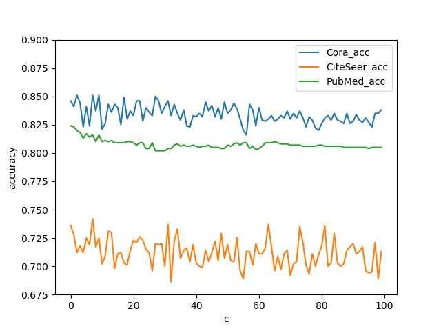
Figure 1: Accuracies of different convexity measures on three datasets.

5 Discussion

5.1 Limitations of EMLP and EGCN

Approximation capability

We can just think the EMLP as just a kind of the neural network and our model EGCN as a kind of GCN but with all the parameters are larger than zero. The parameters are all limited in the open half space when we train the EGCN which means the approximation capability of EGCN is lower than GCN. The limitaion will cause problems such as the train loss will be much large and the predicted values will deviate much from the real values when the parameters of the trained GCN are mostly less than zero and the parameters of the trained EGCN are mostly be close to negative infinity. Thus, only when the parameters of the trained GCN are mostly nonnegative, the model EGCN can make a satisfactory solution.

Convexity limits

To get the convexity of the loss function, we give many limits. one of the limits of input is that $\boldsymbol{x}>\boldsymbol{0}$ which is a very strict restriction that in many dataset, input can’t meet with it. The activation function that meets with condition is also infrequent. Besides, when training EGCN, it may happen that the value is out of range.

5.2 Future work

We hope that we can make more kinds of PCNN besides EMLP and EGCN and transform other neural network to be equiped with convexity such as CNN. For EMLP and EGCN, we can think deeply how to reduce of the limited conditions of convexity. At the same time, we can also reflect on how to enhance approximation capability.

6 Conclusion

In this paper, we transform the neural network to be a convex function of the parameters which is the first convex neural network in our opinion. Besides, we introduce the concept of PCNN and propose the general technique to make two classes of PCNN: EMLP and EGCN and do experiments on graph classification datasets which perform better than GCN and GAT.

References

- Allen-Zhu et al. [2019] Zeyuan Allen-Zhu, Yuanzhi Li, and Zhao Song. A convergence theory for deep learning via over-parameterization. In International Conference on Machine Learning, pages 242–252. PMLR, 2019.
- Boob and Lan [2017] Digvijay Boob and Guanghui Lan. Theoretical properties of the global optimizer of two layer neural network. arXiv preprint arXiv:1710.11241, 2017.
- Chizat and Bach [2018] Lenaic Chizat and Francis Bach. On the global convergence of gradient descent for over-parameterized models using optimal transport. Advances in neural information processing systems, 31, 2018.
- Dauphin et al. [2014] Yann N Dauphin, Razvan Pascanu, Caglar Gulcehre, Kyunghyun Cho, Surya Ganguli, and Yoshua Bengio. Identifying and attacking the saddle point problem in high-dimensional non-convex optimization. Advances in neural information processing systems, 27, 2014.
- Defferrard et al. [2016] Michaël Defferrard, Xavier Bresson, and Pierre Vandergheynst. Convolutional neural networks on graphs with fast localized spectral filtering. Advances in neural information processing systems, 29, 2016.
- Du et al. [2018] Simon S Du, Xiyu Zhai, Barnabas Poczos, and Aarti Singh. Gradient descent provably optimizes over-parameterized neural networks. arXiv preprint arXiv:1810.02054, 2018.
- Du et al. [2019] Simon Du, Jason Lee, Haochuan Li, Liwei Wang, and Xiyu Zhai. Gradient descent finds global minima of deep neural networks. In International conference on machine learning, pages 1675–1685. PMLR, 2019.
- Guo et al. [2017] Huifeng Guo, Ruiming Tang, Yunming Ye, Zhenguo Li, and Xiuqiang He. Deepfm: a factorization-machine based neural network for ctr prediction. arXiv preprint arXiv:1703.04247, 2017.
- Haeffele and Vidal [2017] Benjamin D Haeffele and René Vidal. Global optimality in neural network training. In Proceedings of the IEEE Conference on Computer Vision and Pattern Recognition, pages 7331–7339, 2017.
- Hinton et al. [2012] Geoffrey Hinton, Li Deng, Dong Yu, George E Dahl, Abdel-rahman Mohamed, Navdeep Jaitly, Andrew Senior, Vincent Vanhoucke, Patrick Nguyen, Tara N Sainath, et al. Deep neural networks for acoustic modeling in speech recognition: The shared views of four research groups. IEEE Signal processing magazine, 29(6):82–97, 2012.
- Kawaguchi and Huang [2019] Kenji Kawaguchi and Jiaoyang Huang. Gradient descent finds global minima for generalizable deep neural networks of practical sizes. In 2019 57th Annual Allerton Conference on Communication, Control, and Computing (Allerton), pages 92–99. IEEE, 2019.
- Kingma and Ba [2014] Diederik P Kingma and Jimmy Ba. Adam: A method for stochastic optimization. arXiv preprint arXiv:1412.6980, 2014.
- Kipf and Welling [2016] Thomas N Kipf and Max Welling. Semi-supervised classification with graph convolutional networks. arXiv preprint arXiv:1609.02907, 2016.
- Krizhevsky et al. [2012] Alex Krizhevsky, Ilya Sutskever, and Geoffrey E Hinton. Imagenet classification with deep convolutional neural networks. Advances in neural information processing systems, 25, 2012.
- Li and Yuan [2017] Yuanzhi Li and Yang Yuan. Convergence analysis of two-layer neural networks with relu activation. Advances in neural information processing systems, 30, 2017.
- Magnus and Neudecker [2019] Jan R Magnus and Heinz Neudecker. Matrix differential calculus with applications in statistics and econometrics. John Wiley & Sons, 2019.
- Monti et al. [2017] Federico Monti, Davide Boscaini, Jonathan Masci, Emanuele Rodola, Jan Svoboda, and Michael M Bronstein. Geometric deep learning on graphs and manifolds using mixture model cnns. In Proceedings of the IEEE conference on computer vision and pattern recognition, pages 5115–5124, 2017.
- Nguyen and Hein [2017] Quynh Nguyen and Matthias Hein. The loss surface of deep and wide neural networks. In International conference on machine learning, pages 2603–2612. PMLR, 2017.
- Sen et al. [2008] Prithviraj Sen, Galileo Namata, Mustafa Bilgic, Lise Getoor, Brian Galligher, and Tina Eliassi-Rad. Collective classification in network data. AI magazine, 29(3):93–93, 2008.
- Sun et al. [2020] Ruoyu Sun, Dawei Li, Shiyu Liang, Tian Ding, and Rayadurgam Srikant. The global landscape of neural networks: An overview. IEEE Signal Processing Magazine, 37(5):95–108, 2020.
- Veličković et al. [2017] Petar Veličković, Guillem Cucurull, Arantxa Casanova, Adriana Romero, Pietro Lio, and Yoshua Bengio. Graph attention networks. arXiv preprint arXiv:1710.10903, 2017.
- Wang and others [2018] Qingcan Wang et al. Exponential convergence of the deep neural network approximation for analytic functions. arXiv preprint arXiv:1807.00297, 2018.
- Wu et al. [2019] Xiaoxia Wu, Simon S Du, and Rachel Ward. Global convergence of adaptive gradient methods for an over-parameterized neural network. arXiv preprint arXiv:1902.07111, 2019.
- Yang et al. [2016] Zhilin Yang, William Cohen, and Ruslan Salakhudinov. Revisiting semi-supervised learning with graph embeddings. In International conference on machine learning, pages 40–48. PMLR, 2016.
- Yun et al. [2017] Chulhee Yun, Suvrit Sra, and Ali Jadbabaie. Global optimality conditions for deep neural networks. arXiv preprint arXiv:1707.02444, 2017.
- Zhou et al. [2021] Mo Zhou, Rong Ge, and Chi Jin. A local convergence theory for mildly over-parameterized two-layer neural network. In Conference on Learning Theory, pages 4577–4632. PMLR, 2021.