Boosting unstable particles

Abstract

In relativity, there is no absolute notion of simultaneity, because two clocks that are in different places can always be desynchronized by a Lorentz boost. Here, we explore the implications of this effect for the quantum theory of unstable particles. We show that, when a wavefunction is boosted, its tails travel one to the past and the other to the future. As a consequence, in the new frame of reference, the particle is in a quantum superposition “decayed + non decayed”, where the property “decayed-ness” is entangled with the position. Since a particle cannot be localised in a region smaller than the Compton wavelength, there is a non-zero lower bound on this effect, which is fundamental in nature. The surprising implication is that, in a quantum world, decay probabilities can never be Lorentz-invariant. We show that this insight was the missing ingredient to reconcile the seemingly conflicting views about time dilation in relativistic quantum mechanics and quantum field theory.

Introduction - The problem of how to rigorously formulate a relativistic quantum theory for unstable particles has been a subject of debate for sixty years Zwanziger (1963); Kawai and Gotō (1969); Weldon (1976); Alicki et al. (1986); Stefanovich (1996); Shirokov (2004, 2005); Stefanovich (2006, 2006); Alavi and Giunti (2015); Urbanowski (2014); Urbanowski and Raczyńska (2014); Urbanowski (2017); Exner (1983); Havlíček and Exner (1973); Stefanovich (2005); Giacosa (2016, 2018); Stefanovich (2018). Although a lot of progress has been made, two fundamental questions still remain unanswered:

• Is it possible for two observers in relative motion to disagree on whether an unstable particle is in a decayed state or not Exner (1983); Havlíček and Exner (1973); Stefanovich (2005); Giacosa (2016)?

• Concerning the decay law of moving particles, are there any quantum corrections to the relativistic dilation of time Shirokov (2004, 2005); Stefanovich (2006, 2006); Alavi and Giunti (2015); Urbanowski (2014)?

Clearly, these questions have very broad relevance, since in highly energetic events (such as supernovae, cosmic-ray showers, accelerator experiments, and the early Universe) unstable particles travel in space with very high speeds Bailey et al. (1977, 1979); Baerwald et al. (2012); Lipari (2012); Farley (2015); Schröder (2017); Jaeckel et al. (2018). The topic also has important implications for neutrino physics, as all constraints on neutrino lifetimes Joshipura et al. (2002); Gomes et al. (2015); Chacko et al. (2021); Moss et al. (2018) have time dilation as an built-in assumption.

The goal of this article is to finally resolve the debate around the above questions, in a way that is both rigorous and intuitive. We will show that the seemingly contradictory results found by many authors Stefanovich (1996); Shirokov (2004, 2005); Stefanovich (2006, 2006); Alavi and Giunti (2015); Urbanowski (2014); Urbanowski and Raczyńska (2014); Urbanowski (2017); Exner (1983); Havlíček and Exner (1973); Stefanovich (2005); Giacosa (2016, 2018); Stefanovich (2018) are a necessary consequence of the relativity of simultaneity (the mechanism by which two clocks are desynchronized in a Lorentz boost Wald (1984); Gourgoulhon (2013); Gavassino (2022)). In a nutshell, we will prove that, when a particle is unstable, position uncertainty is Lorentz-transformed into “decayed-ness” uncertainty, because the simultaneity hyperplane is redefined. As a consequence, the decay probability is not a Lorentz scalar.

Throughout the paper, we adopt the signature $(-,+,+,+)$ and work in natural units $c=\hbar=1$. For exposition purposes, we take the neutron, which is unstable to $\beta$-decay

$$n\rightarrow p^{+}+e^{-}+\bar{\nu}_{e}\,,$$ (1)

as our reference particle. However, our results can be straightforwardly generalised to any unstable particle.

The “Alavi-Giunti argument” - It is useful, as a first step, to review a couple of apparently contradictory arguments, which are actually the key to understanding our article. The first argument is due to Alavi and Giunti (2015). According to them, “being a neutron”, or “being a proton + an electron + a neutrino”, are absolute factual truths (valid in all reference frames), because neutrons and, e.g, protons have very different observational signatures. They reason that, if a neutron passes through a detector, it leaves a different track with respect to a proton, and such track can be seen by all observers, independently from their state of motion.

Let us make this argument a little more formal, by considering a concrete observable. The electric four-current $j^{\mu}(x)$ transforms under a Lorentz boost $\Lambda$ as below :

$$U^{\dagger}(\Lambda)j^{\mu}(x)U(\Lambda)=\Lambda\indices{{}^{\mu}_{\rho}}\,j^{\rho}(\Lambda^{-1}x)\,.$$ (2)

Here, ${U}(\Lambda)$ is the unitary representation of $\Lambda$. Averaging (2) over a state $\ket{\alpha}$, defining $\ket{\Lambda\alpha}:={U}(\Lambda)\ket{\alpha}$, and setting $x=0$, we obtain

$$\bra{\Lambda\alpha}j^{\mu}(0)\ket{\Lambda\alpha}=\Lambda\indices{{}^{\mu}_{\rho}}\bra{\alpha}j^{\rho}(0)\ket{\alpha}\,.$$ (3)

Now, it is evident that, if $\ket{\alpha}$ models an isolated neutron at rest near the origin, it will impress a characteristic “neutronic footprint” on $\bra{\alpha}j^{\rho}\ket{\alpha}$. In fact, a neutron does not have a net charge, but it carries a measurable Ampèrian magnetic moment (i.e., a closed of loop of electric current Jackson (1977); Boyer (1988); Mezei (1988); Zyla et al. (2020)). On the other hand, equation (2) tells us that, when we make a Lorentz boost, the quantum average of the electric four-current transforms like a classical vector. Hence, the boost sets the magnetic moment in motion. But this implies that we cannot interpret the state $\ket{\Lambda\alpha}$ as $p^{+}+e^{-}+\bar{\nu}_{e}$, because two sharply separated charges (the proton and the electron) cannot be confused with a single (connected ) loop of electric four-current. Thus, a neutron in proximity of the origin is “perceived as a neutron” by all observers who sit in the origin, independently from their state of motion.

The “Exner-Stefanovich theorem” - There is a simple mathematical theorem Exner (1983); Havlíček and Exner (1973); Stefanovich (2005) that seems to contradict the reasoning above. Let’s take a look at it. Suppose that there is a projector $\mathcal{Q}$, which returns “$\,1\,$” if the state models a neutron, and “$\,0\,$” otherwise. If $K_{1}$ is the generator of the boosts in the direction $1$, and $P^{1}$ is the first component of the four-momentum, we can write down the Jacobi identity:

$$[{\mathcal{Q}},[{K}_{1},{P}^{1}]]+[{K}_{1},[{P}^{1},{\mathcal{Q}}]]+[{P}^{1},[{\mathcal{Q}},{K}_{1}]]=0\,.$$ (4)

On the other hand, $[{K}_{1},{P}^{1}]=i{H}$, where $H$ is the Hamiltonian Weinberg (1995). Furthermore, if a state $\ket{\alpha}$ has a certain probability of being a neutron, the state $e^{-iP^{j}a_{j}}\ket{\alpha}$, which is just a copy of $\ket{\alpha}$ translated in space, should have exactly the same probability of being a neutron. Hence, $\mathcal{Q}$ is invariant under space translations:

$$e^{iP^{j}a_{j}}\,\mathcal{Q}\,e^{-iP^{j}a_{j}}=\mathcal{Q}\quad\quad\quad(\forall\,a_{j}\in\mathbb{R}^{3})\,.$$ (5)

This implies that $[P^{j},\mathcal{Q}]=0$, and equation (4) becomes

$$i[{H},{\mathcal{Q}}]=[{P}^{1},[{\mathcal{Q}},{K}_{1}]]\,.$$ (6)

Since the neutron decays, the operator ${\mathcal{Q}}$ cannot be a conserved quantity. Therefore, $[{H},{\mathcal{Q}}]\neq 0$. It follows from equation (6) that also $[\mathcal{Q},K_{1}]\neq 0$, which implies

$$U^{\dagger}(\Lambda)\,\mathcal{Q}\,U(\Lambda)\neq\mathcal{Q}\,.$$ (7)

This is telling us that, if $\ket{\alpha}$ is a neutron, it is not guaranteed that also $\ket{\Lambda\alpha}$ will be a neutron. This seems to be in stark contrast with the argument of Alavi and Giunti (2015). But, is there really a contradiction?

A thought experiment - Consider the following experimental set up. In Alice’s frame, $\{t_{A},x_{A}^{j}\}$, there are two small boxes at rest, which are kept closed. One box is located at $x_{A}^{1}=0$. The other box is located at $x_{A}^{1}=-L$, where $L>0$ is a very large distance. At $t_{A}=0$, a neutron $n$ is in a pure state $\ket{\psi}$, with $1/2$ probability of being in one box, and $1/2$ probability of being in the other box:

$$\ket{\psi}=\dfrac{\ket{n\text{ in box ``}{-L}\text{''}}+\ket{n\text{ in box ``}0\text{''}}}{\sqrt{2}}\,.$$ (8)

After some time (say, $T=\text{``}5\text{ lifetimes of }n\text{''}$), the neutron is transformed, by unitary evolution, into $p^{+}+e^{-}+\bar{\nu}_{e}$, inside both boxes, with probability $1-e^{-5}\approx 1$. Hence,

$$e^{-i{H}T}\!\ket{\psi}\approx\dfrac{\ket{p,e,\bar{\nu}\text{ in box ``}{-L}\text{''}}+\ket{p,e,\bar{\nu}\text{ in box ``}0\text{''}}}{\sqrt{2}}\,.$$ (9)

The Minkowski diagram of this process is shown in figure 1.

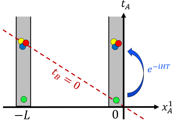
Figure 1: Minkowski diagram of our thought experiment. In Alice’s frame, there is $\{1/2,1/2\}$ probability of having a neutron (green circles) in either of two boxes (grey areas), at $t_{A}=0$. After a time $T$, the neutron decays into $p^{+}+e^{-}+\bar{\nu}_{e}$ (blue+yellow+red circles) in both boxes. Bob moves with velocity $-v$ with respect to Alice. His line of contemporary events (red dashed line) is oblique, and intersects the two boxes at two different times for Alice. As a consequence, in Bob’s frame there is $1/2$ probability of having a neutron in the right box, and $1/2$ probability of having a proton, an electron, and a neutrino in the left box. Therefore, the Lorentz boost has entangled two observables: the neutron projector $\mathcal{Q}$, and the position of the center of mass of the system.

Now, suppose that Bob moves with velocity $-v$ with respect to Alice, and assume that $vL\equiv T$. What is the state of the neutron in Bob’s frame at $t_{B}=0$, assuming that Bob is in the origin? The hyperplane $\{t_{B}=0\}$ coincides with the hyperplane $\{t_{A}=-vx_{A}^{1}\}$, and is plotted in figure 1. As we can see, it intersects the two boxes at two different Alice’s times. In particular, the left box intersects the hyperplane in the event $(T,-L)$, while the right box intersects the hyperplane in the origin. On the other hand, we know that at $(T,-L)$ the neutron has decayed, while in the origin it has not decayed yet. Therefore, if $\Lambda$ is the boost that connects Alice and Bob, namely

$$\Lambda=\begin{bmatrix}\gamma&\gamma v\\ \gamma v&\gamma\\ \end{bmatrix},$$ (10)

we can write

$$U(\Lambda)\ket{\psi}\approx\dfrac{\ket{p,e,\bar{\nu}\text{ in box ``}{-L}\text{''}}+\ket{n\text{ in box ``}0\text{''}}}{\sqrt{2}}\,.$$ (11)

Recalling the definition of $\mathcal{Q}$, we immediately see that

$$1=\bra{\psi}\mathcal{Q}\ket{\psi}\neq\bra{\psi}U^{\dagger}(\Lambda)\,\mathcal{Q}\,U(\Lambda)\ket{\psi}\approx\dfrac{1}{2}\,.$$ (12)

The physical meaning of equation (7) is finally clarified: in the relativistic transformation of time, $t_{B}=\gamma(t_{A}+vx_{A}^{1})$, the term “$\,vx_{A}^{1}\,$” can convert future events into present events, anticipating a decay. This effect becomes stronger the further the particle is from the origin. As a consequence, in equation (11), the “decayed-ness” is correlated with the position. Measuring which box is heavier (i.e. where the particles are) automatically collapses the wavefunction into a state in which the neutron has decayed with a probability that is either $0$ or $1$.

Note that the present thought experiment does not contradict the argument of Alavi and Giunti (2015): if two observers look at the same spacetime event, they agree on whether such event contains a neutron or its decay products (because a loop of four-current cannot be Lorentz-transformed into two point charges). On the other hand, by relativity of simultaneity, two observers can disagree on whether that specific event belongs to the past, present, or future. This is the physical mechanism by which a boost can effectively “cause a decay”.

A more formal proof - For completeness, we provide here a more formal derivation of equation (11). Suppose that $\ket{\alpha}$ models a neutron at rest in the origin. Then, $\bra{\alpha}\mathcal{Q}\ket{\alpha}=1$. Since the origin is a fixed point of Lorentz boosts ($\Lambda 0=0$), we can invoke the argument of Alavi and Giunti (2015), and assume that $\ket{\Lambda\alpha}={U}(\Lambda)\ket{\alpha}$ is still a neutron: $\bra{\Lambda\alpha}\mathcal{Q}\ket{\Lambda\alpha}\approx 1$. Now, let’s consider the state

$$\ket{\Lambda\beta}:=U(\Lambda)\ket{\beta}\,,\quad\text{with}\quad\ket{\beta}:=e^{iP^{1}L}\ket{\alpha}\,.$$ (13)

Using the transformation law of the four-momentum Srednicki (2007),

$$U(\Lambda)\begin{bmatrix}H\\ P^{1}\\ \end{bmatrix}U^{\dagger}(\Lambda)=\Lambda^{-1}\begin{bmatrix}H\\ P^{1}\\ \end{bmatrix}=\gamma\begin{bmatrix}H-vP^{1}\\ P^{1}-vH\\ \end{bmatrix}\,,$$ (14)

we can rewrite $\ket{\Lambda\beta}$ as follows:

$$\ket{\Lambda\beta}=U(\Lambda)e^{iP^{1}L}\ket{\alpha}=e^{iP^{1}\gamma L}e^{-iH\gamma vL}\ket{\Lambda\alpha}\,.$$ (15)

Averaging $\mathcal{Q}$ over $\ket{\Lambda\beta}$, and recalling equation (5), we obtain

$$\bra{\Lambda\beta}\mathcal{Q}\ket{\Lambda\beta}=\bra{\Lambda\alpha}e^{iH\gamma vL}\mathcal{Q}e^{-iH\gamma vL}\ket{\Lambda\alpha}\xrightarrow{L\to\infty}0\,.$$ (16)

As we can see, combining a translation of $-L$, and a boost with velocity $v$, “moves” the neutron forward in time of an amount $\gamma vL$, causing a decay, for large $L$. Ultimately, this is also the physical meaning of equation (6): “time evolution” (left-hand side) is the result of combining a space translation and a boost (right-hand side) Keister and Polyzou (1991).

Now, to recover equation (11), we can just invoke the linearity of $U(\Lambda)$, and make the identification

$$\ket{\psi}\equiv\dfrac{\ket{\beta}+\ket{\alpha}}{\sqrt{2}}\,.$$ (17)

Also, note that the event $(0,-L)$ occurs, in Bob’s frame, at time $t_{B}=-\gamma vL$, so that (16) is geometrically consistent with the Minkowski diagram in figure 1.

Sometimes the decay is inescapable - In the previous section, we “cheated” a bit. In fact, we considered a state $\ket{\alpha}$ that models a neutron “in the origin”. But there is a problem: there is always a little uncertainty $\Delta x^{1}$ about the position of a particle. Therefore, when we boost any wavefunction, its tails (no matter how short) are pushed one to the future and the other to the past, causing a little decay. How important is this effect?

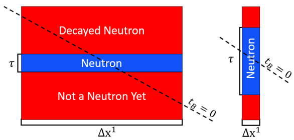
Figure 2: Minkowski diagrams of the wavefunction of a neutron for two different values of the ratio $\Delta x^{1}/\tau$. Left diagram: if $\Delta x^{1}\gg\tau$, the hypersurface $\{t_{B}=0\}$ of a moving observer (dashed line) covers a large region of spacetime where the particle is not a neutron (in red), so that $\bra{\Lambda\alpha}\mathcal{Q}\ket{\Lambda\alpha}\ll 1$. Right diagram: the condition $\Delta x^{1}\ll\tau$ restores $\bra{\Lambda\alpha}\mathcal{Q}\ket{\Lambda\alpha}\approx 1$, because the hypersurface $\{t_{B}=0\}$ intersects only the “neutron region” (in blue).

Suppose that $\ket{\alpha}$ is a neutron wavepacket with center in the origin and zero average velocity. By contraction of lengths, the tails of the wavefunction $\ket{\Lambda\alpha}$ extend till $|x^{1}|\sim\Delta x^{1}/\gamma$. To estimate the tail “desynchronization”, we can just evaluate equation (2) on one tail (for $t=0$):

$$\bra{\Lambda\alpha}j^{\mu}(0,\Delta x^{1}/\gamma)\ket{\Lambda\alpha}=\Lambda\indices{{}^{\mu}_{\rho}}\bra{\alpha}j^{\rho}(-v\Delta x^{1},\Delta x^{1})\ket{\alpha}\,.$$ (18)

Comparing the times at which $j$ is evaluated, we can conclude that the desynchronization timescale between $\ket{\alpha}$ and $\ket{\Lambda\alpha}$ is $\Delta t\sim v\,\Delta x^{1}$. If this timescale becomes comparable to the decay time $\tau$, the neutron decays along the tails of the wavefunction, just by relativity of simultaneity. To avoid this possibility for all values of $v$, we must require that (see also figure 2)

$$\Delta x^{1}\ll\tau\,.$$ (19)

This is the central inequality of the paper: when it is respected, one has $\bra{\Lambda\alpha}\mathcal{Q}\ket{\Lambda\alpha}\approx 1$, provided that the wavepacket is centered in the origin. This is also confirmed by the explicit calculation of Stefanovich (2005). However, if (19) is broken, a boost causes a measurable decay, no matter where we set the origin! Of course, an example of a state that violates (19) is the state $\ket{\psi}$ of our thought experiment (see figure 1).

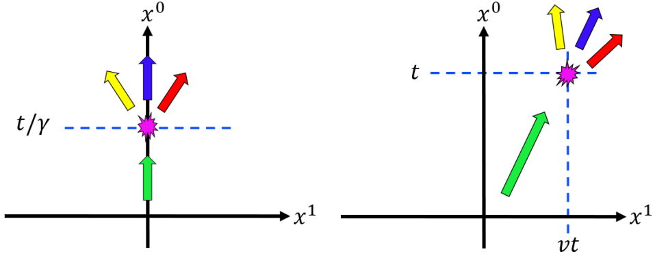
Figure 3: Minkowski diagrams of $\bra{\beta}e^{-iHt/\gamma}\ket{\alpha}$ (left panel) and $\bra{\Lambda\beta}e^{iP^{1}vt}e^{-iHt}\ket{\Lambda\alpha}$ (right panel). The two processes are mapped into each other by a Lorentz boost. As a consequence, the value of the probability amplitude is exactly the same. Everything goes as Special Relativity predicts: when we boost, $t/\gamma$ is “stretched” into $t$ (time dilation). The translation $e^{i\hat{P}^{1}vt}$ is necessary: the boosted neutron travels a distance $vt$ before decaying, so that we must project on $e^{-i\hat{P}^{1}vt}\ket{\Lambda\beta}$, not on $\ket{\Lambda\beta}$.

In the Appendix, we compute explicitly the average $\bra{\Lambda\alpha}\mathcal{Q}\ket{\Lambda\alpha}$, under the assumption that $\ket{\alpha}$ is a Gaussian wavepacket (at rest in the origin) with $\bra{\alpha}\mathcal{Q}\ket{\alpha}=1$. We obtain the approximate formula below:

$$\bra{\Lambda\alpha}\mathcal{Q}\ket{\Lambda\alpha}\approx e^{a^{2}}\text{erfc}|a|\quad\text{with }a:=\dfrac{v\Delta x^{1}}{\tau\sqrt{2}}\,,$$ (20)

where “ erfc ” is the complementary error function. As expected, if (19) is obeyed (i.e. $a\rightarrow 0$), the above expression converges to $1$. But if (19) is violated, then $\bra{\Lambda\alpha}\mathcal{Q}\ket{\Lambda\alpha}\sim a^{-1}$, which tends to zero for large $a$.

Now, there is an important fact to note. A particle cannot be localised in a region of space that is smaller than the Compton wavelength $M^{-1}$ Berestetskii et al. (1973); Kaloyerou (1988); Eberhard and Ross (1989); Barat and Kimball (2003). Therefore, a single-particle state that obeys (19) is allowed to exist only if $M^{-1}\ll\tau$. As a consequence, we can always find two observers that disagree on whether a “resonance particle”, with $M^{-1}\sim\tau$ (i.e. $M\sim\Gamma:=\tau^{-1}$ Alavi and Giunti (2015)), exists or not. In other words, the inequality $M^{-1}\ll\tau$ is a necessary (but not sufficient!) condition for establishing the (approximate) Lorentz-invariance of $\braket{\mathcal{Q}}$.

Quantum deviations from time dilation - We are finally able to discuss the problem of time dilation. We first summarize the state of the art. Let $\ket{\chi}$ be an isolated neutron in an arbitrary state of motion. Since it is a neutron with probability $1$, we know that $\bra{\chi}\mathcal{Q}\ket{\chi}=1$. We let it evolve for a time $t$. The state now is $e^{-iHt}\ket{\chi}$, and the probability that we still have a neutron is

$$\mathcal{P}(t)=\bra{\chi}e^{iHt}\mathcal{Q}e^{-iHt}\ket{\chi}\,.$$ (21)

Since $\mathcal{Q}$ and $P^{j}$ are commuting observables, they can be diagonalised simultaneously. Thus, there is a set of neutron momentum eigenstates $\ket{n,\textbf{p},\sigma}$ such that ($\sigma$ is the spin)

$$\begin{split}{\mathcal{Q}}\ket{n,\textbf{p},\sigma}={}&\ket{n,\textbf{p},\sigma}\,,\\ {P}^{j}\ket{n,\textbf{p},\sigma}={}&p^{j}\ket{n,\textbf{p},\sigma}\,.\\ \end{split}$$ (22)

One can expand $\mathcal{Q}$ and $\ket{\chi}$ using these states. All that remains is to calculate the characteristic amplitudes

$$\mathcal{A}(t)=\bra{n,\textbf{p},\sigma}e^{-iHt}\ket{n,\textbf{p},\sigma}\,.$$ (23)

Let us jump directly to the result. Depending on the level of detail, the exact formula may change slightly, but all authors agree Shirokov (2005); Stefanovich (2006); Urbanowski (2014); Giacosa (2016) that the decay timescale of a neutron with momentum p can be expressed as

$$\tau(\textbf{p})=\tau\,\dfrac{\sqrt{M^{2}+\textbf{p}^{2}}}{M}\bigg{[}1+\mathcal{O}\bigg{(}\dfrac{M^{-1}}{\tau}\bigg{)}\bigg{]}\,.$$ (24)

Outside the bracket, we have the usual time-dilated decay time “$\,\tau\gamma\,$”. The bracket is a pure quantum correction, which deviates from 1 only when the Compton wavelength $M^{-1}$ is comparable to the rest-frame decay time $\tau$. This correction has been a source of debate for a long time: is it just a mathematical artefact Alavi and Giunti (2015), or are we observing a breakdown of Special Relativity (SR) Stefanovich (2005)? As we are going to show, neither. This effect is physical, and it does not contradict SR.

First, let us consider the identity below:

$$e^{-iHt/\gamma}=U^{\dagger}(\Lambda)e^{iP^{1}vt}e^{-iHt}U(\Lambda)\,.$$ (25)

It can be easily proved by inverting equation (14). Its matrix element between two generic states $\bra{\beta}$ and $\ket{\alpha}$ is

$$\bra{\beta}e^{-iHt/\gamma}\ket{\alpha}=\bra{\Lambda\beta}e^{iP^{1}vt}e^{-iHt}\ket{\Lambda\alpha}\,.$$ (26)

To understand the physical meaning of this exact identity, consider the case in which $\ket{\alpha}$ is a neutron at rest near the origin, and $\ket{\beta}$ is a triplet $p^{+}+e^{-}+\bar{\nu}_{e}$. Then, the amplitudes above can be schematically plotted in a “Feynman-Minkowski” diagram, as in figure 3. As we can see, the phenomenon of time dilation is perfectly well captured by the quantum theory: the amplitude for $\ket{\alpha}$ to transform into $\ket{\beta}$ in a time $t/\gamma$ is equal to the amplitude for $\ket{\Lambda\alpha}$ to transform into $e^{-i\hat{P}^{1}vt}\ket{\Lambda\beta}$ in a (longer) time $t$. There is no “quantum breakdown of SR”.

However, there is a complication. If $M^{-1}\gtrsim\tau$, then it is impossible for $\ket{\alpha}$ to obey (19) without breaking the Compton limit ($\Delta x^{1}\gtrsim M^{-1}$). As a result, if $\ket{\alpha}$ is a neutron, in the sense that $\bra{\alpha}\mathcal{Q}\ket{\alpha}=1$, then in general $\ket{\Lambda\alpha}$ is not a perfect neutron: $\bra{\Lambda\alpha}\mathcal{Q}\ket{\Lambda\alpha}<1$. Thus, we cannot construct moving neutron states by applying Lorentz boosts to neutrons at rest. Vice versa, if we take a moving neutron, and we boost to its rest frame, we no longer have a neutron. This implies that the mathematical identity (26) cannot be used to relate the decay amplitude of a neutron at rest with that of a neutron in motion, because $\ket{\Lambda\alpha}$ (the “boosted neutron”) and $\ket{\chi}$ (the moving neutron) are different states!

On the other hand, if $M^{-1}\ll\tau$, then it is possible to construct couples of states $\ket{\alpha}$ and $\ket{\Lambda\alpha}$ that are both neutrons, because (19) does not violate the Compton limit. Now yes: we can use (26) to relate the decay amplitudes for neutrons in different states of motion, and time dilation must be restored. This explains why the quantum correction in (24) tends to zero in this limit. Indeed, in their derivation of time dilation, Alavi and Giunti (2015) were forced to assume that $M^{-1}\ll\Delta x^{1}\ll\tau$.

In conclusion, equation (20) acts as a bridge between the analysis of Alavi and Giunti (2015) and the theorem of Exner (1983) and Stefanovich (2005). In fact, in the regime considered by Alavi-Giunti (namely, $\Delta x^{1}\ll\tau$), equation (20) reduces to $\bra{\Lambda\alpha}\mathcal{Q}\ket{\Lambda\alpha}\approx 1$, restoring our intuition that a neutron is perceived as a neutron in all reference frames. On the other hand, when $\Delta x^{1}$ becomes comparable to $\tau$, the operator $\mathcal{Q}$ ceases to be Lorentz-invariant, and $\bra{\Lambda\alpha}\mathcal{Q}\ket{\Lambda\alpha}<1$, in agreement with the Exner-Stefanovich theorem.

Application 1: neutrino decay - Massive neutrinos may decay, and there are many possible decay channels outside the standard model Gomes et al. (2015). As a proof of principle, let us see what happens if the heaviest neutrino has mass $M=0.05\,$eV and rest-frame decay time $\tau=10^{-13}\,$s (such extremely short lifetime is consistent with observational constraints Gomes et al. (2015)). With the choice of parameters above, we get $M^{-1}/\tau\approx 0.83$. Hence, time dilation breaks down completely [see equation (24)]. This is a serious problem, because all constraints on the neutrino lifetime assume from the start that time dilation is valid Baerwald et al. (2012). Furthermore, if we set $\Delta x^{1}\approx M^{-1}$ and $v\approx 1$ in (20), we obtain $\bra{\Lambda\alpha}\mathcal{Q}\ket{\Lambda\alpha}\approx 0.57$, meaning that a boosted neutrino has only $57\%$ of probability of existing as a neutrino!

Application 2: sterile neutrinos - Moss et al. (2018) consider a hypothetical sterile neutrino species, $\nu_{4}$, with very short lifetime: $\tau\approx 10^{-16}\,$s. Taking again $v\sim 1$ and $\Delta x^{1}\approx M^{-1}$, and assuming $M=1\,$eV, we obtain $\bra{\Lambda\alpha}\mathcal{Q}\ket{\Lambda\alpha}\approx 0.02$. This means that such sterile neutrino disappears almost completely when we boost it.

Application 3: boosting pions - The lifetime of the neutral pion, $\pi^{0}$, is $\tau\approx 8.5\times 10^{-17}\,$s Zyla et al. (2020). If we apply an ultra-relativistic boost ($v\sim 1$) to a wavefunction having rest-frame position uncertainty $\Delta x^{1}\approx 5\times 10^{-8}\,$m, we obtain $\bra{\Lambda\alpha}\mathcal{Q}\ket{\Lambda\alpha}\approx 0.34$. Whether values of $\Delta x^{1}$ of the order of $10^{-8}\,$m are actually attained in experiments will be subject of future investigation (note that in the laboratory frame the position uncertainty is shorter of a factor $1/\gamma$ ). But if this happens, an ultra-relativistic $\pi^{0}$ exists only with probability $\sim 1/3$, provided that its existence probability is $1$ in the rest frame.

Future perspectives - The role that relativity of simultaneity can play in the quantum dynamics of an unstable system has been overlooked till now . Here, we were focusing on what happens when we boost a single unstable particle. However, also larger systems should exhibit such counterintuitive effects. It would be interesting to apply this same set of ideas to an unstable field Lima (2013), and see if similar “paradoxes” occur. We leave this as a subject of future investigation.

-
L.G. acknowledges support by the Polish National Science Centre grant OPUS 2019/33/B/ST9/00942. F. G. acknowledge support from the Polish National Science Centre grant OPUS 2019/33/B/ST2/00613.

APPENDIX

I A simple formula

In this section, we derive a simple analytical formula for the probability $\mathcal{P}(t=0)=\bra{\Lambda\alpha}\mathcal{Q}\ket{\Lambda\alpha}$ that a boosted neutron (located nearby the origin) is still a neutron (at $t=0$). It is only a rough estimate, but it is important to have an expression that can be used in “back-of-the-envelope calculations”. For simplicity, we work in 1+1 dimensions.

We start from a simple observation: if there is only one baryon, the projector $\mathcal{Q}$ may be interpreted as the “neutron number”, namely an effective (non-conserved) charge that counts “how many neutrons are there”, across all space. A quantum number of this kind can be expressed (see Section 15.8 of Bjorken and Drell (1965)) as the flux of some associated current $J^{\nu}$ through hyperplanes $\{\text{time}=\text{const}\}$, namely

$$\mathcal{Q}=\int_{t=\text{const}}\!\!\!\!\!\!\!\!\!d\Sigma_{\nu}\,J^{\nu}=\int dx\,J^{0}\,.$$ (27)

The decay of the neutron is possible because $J^{\nu}$ is not a Noether current of the field theory, so that $\partial_{\nu}J^{\nu}\neq 0$, and

$$\dfrac{d\mathcal{Q}}{dt}=\int dx\,\partial_{t}J^{0}=\int dx\,\partial_{\nu}J^{\nu}\neq 0\,.$$ (28)

We can immediately see the problem: the standard proof of the Lorentz-invariance of a charge Weinberg (1972) makes explicit use of the condition $\partial_{\nu}J^{\nu}=0$. In fact, one has to apply the Gauss theorem in the spacetime volume enclosed by the surfaces of constant time of Alice and Bob, which are tilted by relativity of simultaneity (see Misner et al. (1973), figure 5.3.c). If $\partial_{\nu}J^{\nu}\neq 0$, Alice and Bob can disagree on the average value of $\mathcal{Q}$. Our goal, now, is to quantify the disagreement.

The state $\ket{\alpha}$ models a Gaussian neutron wavepacket at rest in the origin. Following Exner (1983), we assume that the wavefunction does not “spread around” over the decay timescale $\tau$ [i.e. $\Delta x(\tau)\approx\Delta x(0)=:\Delta x$], and we postulate (for simplicity) a purely exponential decay law. Then, working in the Heisenberg picture, we can write

$$\bra{\alpha}J^{0}(t,x)\ket{\alpha}\approx\dfrac{e^{-|t|/\tau}}{\sqrt{2\pi}\,\Delta x}\exp\bigg{[}-\dfrac{x^{2}}{2\Delta x^{2}}\bigg{]}\,,\quad\quad\quad\bra{\alpha}J^{1}(t,x)\ket{\alpha}\approx 0\,.$$ (29)

This expression is not extremely accurate, but it “captures the essence”. In particular, if the neutron does not decay ($\tau=+\infty$), we recover $\bra{\alpha}\partial_{\nu}J^{\nu}\ket{\alpha}=0$. But if the neutron decays (finite $\tau$), then $\bra{\alpha}\partial_{\nu}J^{\nu}\ket{\alpha}=\partial_{t}\bra{\alpha}J^{0}\ket{\alpha}\neq 0$. Note the presence of the absolute value in the time-dependence: equation (29) is valid also for negative times. To see that $e^{-|t|/\tau}$ is the correct time-dependence for all $t\in\mathbb{R}$ (also negative), one can just invoke the Breit-Wigner formula, for a particle (at rest) with mass $M$ and decay rate $\Gamma=\tau^{-1}\,$:

$$\bra{\alpha}e^{iHt}\mathcal{Q}e^{-iHt}\ket{\alpha}\,\,\overset{\text{B.W.}}{\approx}\,\,\bigg{|}\int\dfrac{dm}{2\pi}\,\dfrac{\Gamma e^{-imt}}{(m-M)^{2}+\Gamma^{2}/4}\bigg{|}^{2}=e^{-|t|/\tau}\,.$$ (30)

Now we only have to boost from the state $\ket{\alpha}$ to the state $\ket{\Lambda\alpha}=U(\Lambda)\ket{\alpha}$. To this end, we need to remember that the current $J^{\nu}$ is a vector field: it transforms according to the formula Srednicki (2007)

$$U^{\dagger}(\Lambda)\begin{bmatrix}J^{0}(t,x)\\ J^{1}(t,x)\\ \end{bmatrix}U(\Lambda)=\gamma\begin{bmatrix}J^{0}(\gamma t-\gamma vx,\gamma x-\gamma vt)+vJ^{1}(\gamma t-\gamma vx,\gamma x-\gamma vt)\\ J^{1}(\gamma t-\gamma vx,\gamma x-\gamma vt)+vJ^{0}(\gamma t-\gamma vx,\gamma x-\gamma vt)\\ \end{bmatrix}\,.$$ (31)

Averaging the zeroth component of the above equation over $\ket{\alpha}$, we obtain

$$\bra{\Lambda\alpha}J^{0}(t,x)\ket{\Lambda\alpha}\approx\dfrac{\gamma\,e^{-\gamma|t-vx|/\tau}}{\sqrt{2\pi}\,\Delta x}\exp\bigg{[}-\dfrac{\gamma^{2}(x-vt)^{2}}{2\Delta x^{2}}\bigg{]}\,.$$ (32)

Evaluating this formula at $t=0$, integrating over $x$, and recalling equation (27), we obtain (assume $v>0$ for clarity)

$$\bra{\Lambda\alpha}\mathcal{Q}\ket{\Lambda\alpha}\approx\int dx\,\dfrac{\gamma\,e^{-\gamma v|x|/\tau}}{\sqrt{2\pi}\,\Delta x}\,\exp\bigg{[}-\dfrac{\gamma^{2}x^{2}}{2\Delta x^{2}}\bigg{]}\,.$$ (33)

Note the presence of the factor $e^{-\gamma v|x|/\tau}\,$: by relativity of simultaneity, the time-dependence coming from $e^{-|t|/\tau}$ has been converted into a space dependence! The above integral can be solved analytically, giving

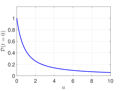
Figure 4: Graph of $\mathcal{P}(t=0)=\bra{\Lambda\alpha}\mathcal{Q}\ket{\Lambda\alpha}$ as a function of the characteristic ratio $a=v\Delta x/\tau\sqrt{2}$. The quantity $\mathcal{P}(t=0)$ expresses the probability that a boosted neutron is detected as neutron (at $t=0$). The deviations of $\bra{\Lambda\alpha}\mathcal{Q}\ket{\Lambda\alpha}$ from $1$ are possible only because the decay in time, $e^{-|t|/\tau}$, is transformed (by relativity of simultaneity) into a decay in space, $e^{-\gamma v|x|/\tau}$. The dimensionless parameter $a$ quantifies the importance of this effect.

$$\mathcal{P}(t=0)=\bra{\Lambda\alpha}\mathcal{Q}\ket{\Lambda\alpha}\approx e^{a^{2}}\text{erfc}(a)\,,\quad\quad\quad\text{with }\,a:=\dfrac{v\,\Delta x}{\tau\sqrt{2}}\,,$$ (34)

where “ erfc ” denotes the complementary error function. We plot (34) in figure 4. As we can see, if $v\rightarrow 0$, or the position uncertainty is small, or the lifetime of the particle is long, then $\bra{\Lambda\alpha}\mathcal{Q}\ket{\Lambda\alpha}\approx 1$. But if the particle is strongly delocalised and short-lived, and $v\sim 1$, the boost causes an effective decay: $\bra{\Lambda\alpha}\mathcal{Q}\ket{\Lambda\alpha}\rightarrow 0$.

Why does $\bra{\Lambda\alpha}\mathcal{Q}\ket{\Lambda\alpha}$ depend only on $a\,$? There is a simple geometrical explanation for that. By length contraction, the uncertainty on the neutron’s position is $\Delta x\,\gamma^{-1}$. On the other hand, the neutron “is really a neutron” only if it is found in a location where the decay factor $e^{-\gamma v|x|/\tau}$ is close to $1\,$, otherwise (instead of detecting a neutron) we detect the decay products of the neutron: $p^{+}+e^{-}+\bar{\nu}_{e}$. Since the decay factor $e^{-\gamma v|x|/\tau}$ falls on a length scale $\tau(\gamma v)^{-1}$, the ratio between $\tau(\gamma v)^{-1}$ and $\Delta x\,\gamma^{-1}$ quantifies the “neutron-ness” of the state $\ket{\Lambda\alpha}$. Such ratio coincides with $a^{-1}$, apart from the factor $\sqrt{2}$. Indeed, in the limit of large $a$, one has the asymptotic behaviour

$$\bra{\Lambda\alpha}\mathcal{Q}\ket{\Lambda\alpha}\approx\dfrac{1}{a\sqrt{\pi}}=\dfrac{\tau\,\sqrt{2}}{v\,\Delta x\,\sqrt{\pi}}\,.$$ (35)

II Direct amplitude calculation

In the previous section, we derived equation (34) by expressing $\mathcal{Q}$ as the charge associated to a non-conserved current $J^{\nu}$. However, decay amplitudes are usually calculated in a different way. Typically, one expands the state $\ket{\alpha}$ in terms of four-momentum eigenstates, and computes the average $\bra{\alpha}e^{iHt}\mathcal{Q}e^{-iHt}\ket{\alpha}$ integrating over the four-momentum eigenbasis. It is natural to ask whether the same strategy can be adopted to compute $\bra{\alpha}U^{\dagger}(\Lambda)\mathcal{Q}U(\Lambda)\ket{\alpha}$. Unfortunately, this kind of calculation leads to very complicated nested integrals in momentum and mass space Stefanovich (2005). Obtaining a simple and transparent formula seems out of the question. However, the qualitative features of (34) remain. This is what we are going to show now. But we must warn the reader: this is a very technical and tedious calculation.

II.1 Completeness relation

First, let us set up some notation. We follow the same strategy of Peskin and Schroeder (1995), Section 7.1, equation (7.2), and we construct the completeness relation below (we work 3+1 dimensions):

$$\mathbb{I}=\ket{\text{VAC}}\bra{\text{VAC}}+\sum_{g}\int\dfrac{d^{3}p}{(2\pi)^{3}}\dfrac{\ket{\,g,\textbf{p}\,}\bra{\,g,\textbf{p}\,}}{2E_{g}(\textbf{p})}\,,$$ (36)

where $\mathbb{I}$ is the identity operator, $\ket{\text{VAC}}$ is the vacuum state, and $\ket{\,g,\textbf{p}\,}$ are four-momentum eigenstates with mass $m_{g}$,

$$P^{j}\ket{\,g,\textbf{p}\,}=p^{j}\ket{\,g,\textbf{p}\,}\quad\quad\quad H\ket{\,g,\textbf{p}\,}=E_{g}(\textbf{p})\ket{\,g,\textbf{p}\,}=\sqrt{m_{g}^{2}+\textbf{p}^{2}}\ket{\,g,\textbf{p}\,}\,.$$ (37)

Consistently with Peskin and Schroeder (1995), we had to include the denominator “$\,2E_{g}(\textbf{p})\,$” in (36), because we are adopting the covariant normalization

$$\braket{\,\tilde{g},\textbf{q}\,}{\,g,\textbf{p}\,}=2E_{g}(\textbf{p})(2\pi)^{3}\delta^{3}(\textbf{q}-\textbf{p})\delta_{\tilde{g},g}\,.$$ (38)

For this choice of normalization, we have the transformation law

$$U(\Lambda)\ket{\,g,\textbf{p}\,}=\ket{\,g,\Lambda\textbf{p}\,}\,,$$ (39)

where the notation “$\,\Lambda\textbf{p}\,$” just means that we construct the four-vector $(E_{g},\textbf{p})$, we boost it, and we take the space part of the boosted vector. In particular, if $\Lambda$ is a boost of velocity $v$ in the $x^{1}$ direction, we have that

$$\Lambda\textbf{p}=(\,\gamma p^{1}{+}\gamma vE_{g}(\textbf{p}),\,p^{2},\,p^{3}\,)\,.$$ (40)

II.2 Neutron projector

For simplicity, we set the neutron’s spin to zero, so that the projector $\mathcal{Q}$ can be expressed as follows:

$$\mathcal{Q}=\int\dfrac{d^{3}p}{(2\pi)^{3}}\ket{\,n,\textbf{p}\,}\bra{\,n,\textbf{p}\,}\,.$$ (41)

The states $\ket{\,n,\textbf{p}\,}$ are not eigenstates of the Hamiltonian, because $[H,\mathcal{Q}]\neq 0$. Hence, we cannot introduce a covariant normalization, like (38), but we need to “stick to the standard one”:

$$\braket{\,n,\textbf{q}\,}{\,n,\textbf{p}\,}=(2\pi)^{3}\delta^{3}(\textbf{q}-\textbf{p})\,.$$ (42)

Note that $\ket{\,n,\textbf{p}\,}$ are exact momentum eigenstates:

$$P^{j}\ket{\,n,\textbf{p}\,}=p^{j}\ket{\,n,\textbf{p}\,}\,.$$ (43)

This is possible because, as we said in the main text, the neutron projector must be invariant under space translations: $[\mathcal{Q},P^{j}]=0$. Comparing (37) and (43), we conclude that

$$\braket{\,g,\textbf{q}\,}{\,n,\textbf{p}\,}=f(g,\textbf{p})\sqrt{2E_{g}(\textbf{p})}\,(2\pi)^{3}\delta^{3}(\textbf{q}-\textbf{p})\,.$$ (44)

where $f(g,\textbf{p})$ is some complex distribution. Clearly, $\mathcal{Q}\ket{\text{VAC}}=0$, which implies $\braket{\,n,\textbf{p}\,}{\text{VAC}}=0$. Therefore, we can use the completeness relation to derive a condition on $\braket{\,g,\textbf{q}\,}{\,n,\textbf{p}\,}$:

$$(2\pi)^{3}\delta^{3}(\textbf{q}-\textbf{p})=\braket{\,n,\textbf{q}\,}{\,n,\textbf{p}\,}=\bra{\,n,\textbf{q}\,}\mathbb{I}\ket{\,n,\textbf{p}\,}=\sum_{g}\int\dfrac{d^{3}k}{(2\pi)^{3}}\dfrac{\braket{\,n,\textbf{q}\,}{\,g,\textbf{k}\,}\braket{\,g,\textbf{k}\,}{\,n,\textbf{p}\,}}{2E_{g}(\textbf{k})}\,.$$ (45)

Invoking (44), this equation reduces to a normalization requirement on $f\,$:

$$\sum_{g}|f(g,\textbf{p})|^{2}=1\quad\quad\quad\forall\,\textbf{p}\in\mathbb{R}^{3}\,.$$ (46)

II.3 Boosted decay law

We are finally ready to compute the formula for the decay law of a boosted neutron state. We start with a neutron state $\ket{\alpha}$, and we introduce the function

$$\alpha(\textbf{p}):=\braket{\,n,\textbf{p}\,}{\alpha}\quad\quad\quad\text{with}\quad\quad\quad\braket{\alpha}{\alpha}=\braket{\alpha}{\mathcal{Q}}{\alpha}=\int\dfrac{d^{3}p}{(2\pi)^{3}}|\alpha(\textbf{p})|^{2}=1\,.$$ (47)

Clearly, if $\ket{\alpha}$ is a neutron with probability $1$, then $\mathcal{Q}\ket{\alpha}=\ket{\alpha}$ and $\braket{\text{VAC}}{\alpha}=0$. As a consequence, we can write the following chain of identities:

$$\ket{\alpha}=\mathbb{I}\mathcal{Q}\ket{\alpha}=\sum_{g}\int\dfrac{d^{3}p}{(2\pi)^{3}}\dfrac{d^{3}q}{(2\pi)^{3}}\dfrac{\ket{\,g,\textbf{p}\,}}{2E_{g}(\textbf{p})}\braket{\,g,\textbf{p}\,}{\,n,\textbf{q}\,}\braket{\,n,\textbf{q}\,}{\alpha}\,.$$ (48)

Using (44) and (47), this simplifies to

$$\ket{\alpha}=\sum_{g}\int\dfrac{d^{3}p}{(2\pi)^{3}}\,\alpha(\textbf{p})\,f(g,\textbf{p})\,\dfrac{\ket{\,g,\textbf{p}\,}}{\sqrt{2E_{g}(\textbf{p})}}\,.$$ (49)

Now, we apply a Lorentz boost and we evolve the resulting state in time:

$$e^{-iHt}U(\Lambda)\ket{\alpha}=\sum_{g}\int\dfrac{d^{3}p}{(2\pi)^{3}}\,\alpha(\textbf{p})\,f(g,\textbf{p})\,\dfrac{e^{-iE_{g}(\Lambda\textbf{p})t}\ket{\,g,\Lambda\textbf{p}\,}}{\sqrt{2E_{g}(\textbf{p})}}$$ (50)

As usual, we introduce the notation $\ket{\Lambda\alpha}:=U(\Lambda)\ket{\alpha}$. Furthermore, we change variable in the integral from p to $\textbf{q}=\Lambda\textbf{p}$, and recall that the invariant volume element in momentum space is

$$\dfrac{d^{3}p}{2E_{g}(\textbf{p})}=\dfrac{d^{3}q}{2E_{g}(\textbf{q})}\,,$$ (51)

so that (50) becomes

$$e^{-iHt}\ket{\Lambda\alpha}=\sum_{g}\int\dfrac{d^{3}q}{(2\pi)^{3}}\dfrac{\sqrt{2E_{g}(\Lambda^{-1}\textbf{q})}}{2E_{g}(\textbf{q})}\,\alpha(\Lambda^{-1}\textbf{q})\,f(g,\Lambda^{-1}\textbf{q})\,e^{-iE_{g}(\textbf{q})t}\ket{\,g,\textbf{q}\,}\,.$$ (52)

Now we can project this state on a generic neutron state $\ket{\,n,\textbf{k}}$. The result is

$$\bra{\,n,\textbf{k}}e^{-iHt}\ket{\Lambda\alpha}=\sum_{g}\sqrt{\dfrac{E_{g}(\Lambda^{-1}\textbf{k})}{E_{g}(\textbf{k})}}\,\alpha(\Lambda^{-1}\textbf{k})\,f(g,\Lambda^{-1}\textbf{k})\,f^{*}(g,\textbf{k})\,e^{-iE_{g}(\textbf{k})t}\,.$$ (53)

The decay law of the state $\ket{\Lambda\alpha}$ is the function

$$\mathcal{P}(t)=\bra{\Lambda\alpha}e^{iHt}\mathcal{Q}e^{-iHt}\ket{\Lambda\alpha}=\int\dfrac{d^{3}k}{(2\pi)^{3}}|\bra{\,n,\textbf{k}\,}e^{-iHt}\ket{\Lambda\alpha}|^{2}\,.$$ (54)

Using equation (53) we finally obtain an integral expression for $\mathcal{P}\,$:

$$\mathcal{P}(t)=\int\dfrac{d^{3}k}{(2\pi)^{3}}\bigg{|}\sum_{g}\sqrt{\dfrac{E_{g}(\Lambda^{-1}\textbf{k})}{E_{g}(\textbf{k})}}\,\alpha(\Lambda^{-1}\textbf{k})\,f(g,\Lambda^{-1}\textbf{k})\,f^{*}(g,\textbf{k})\,e^{-iE_{g}(\textbf{k})t}\bigg{|}^{2}\,.$$ (55)

This formula generalizes equation (13.75) of Stefanovich (2005), and it is essentially exact: it is valid in any relativistic quantum theory, including QFT. The only approximation is that we have neglected the spin of the neutron. Note that the function $\alpha$ cannot be taken out of the summation, because the notation “$\,\Lambda^{-1}\textbf{k}\,$” stands for [see equation (40)]

$$\Lambda^{-1}\textbf{k}=(\,\gamma k^{1}{-}\gamma vE_{g}(\textbf{k}),\,k^{2},\,k^{3}\,)\,,$$ (56)

and depends on $g$ through $E_{g}$.

II.4 A quick check: space-translated states

Before studying the dependence of $\mathcal{P}(0)$ on the position uncertainty, let us see what happens if we replace the state $\ket{\alpha}$ with $\ket{\beta}=e^{iP^{1}L}\ket{\alpha}$. First of all, we note that

$$\beta(\textbf{p})=\bra{\,n,\textbf{p}\,}e^{iP^{1}L}\ket{\alpha}=e^{ip^{1}L}\alpha(\textbf{p})\,.$$ (57)

Thus, in equation (55), we just need to replace “$\,\alpha(\Lambda^{-1}\textbf{k})\,$” with

$$\beta(\Lambda^{-1}\textbf{k})=e^{ik^{1}\gamma L}e^{-iE_{g}(\textbf{k})\gamma vL}\alpha(\Lambda^{-1}\textbf{k})\,.$$ (58)

Now, the factor $e^{ik^{1}\gamma L}$ does not depend on $g$. Thus, in equation (55), we can take it out of the summation over $g$, and the absolute value cancels it. The factor $e^{-iE_{g}(\textbf{k})\gamma vL}$, on the other hand, depends on $g$, and it can be combined with the exponential $e^{-iE_{g}(\textbf{k})t}$. The result is that the decay law of $\ket{\Lambda\beta}$ can be obtained directly from the decay law of $\ket{\Lambda\alpha}$, equation (55), just making the replacement

$$t\longrightarrow t+\gamma vL\,.$$ (59)

This is in perfect agreement with our results of the main text: “space translation + boost = time evolution”. From equation (55), we can easily see what happens if we take the limit of large $L$: the exponential $e^{-iE_{g}(\textbf{k})\gamma vL}$ becomes highly oscillating, and the contributions coming from all possible values of $g$ (which give rise to a continuum of energies) average to zero, leading to a decay.

II.5 A couple of simplifications

Let us go back to $\mathcal{P}(t)=\bra{\Lambda\alpha}e^{iHt}\mathcal{Q}e^{-iHt}\ket{\Lambda\alpha}$. Stefanovich (2005) has shown, using equation (55), that if $\Delta x^{1}\ll\tau$ (equivalently, $a\rightarrow 0$), and the wavepacket is not too far from the origin, then $\mathcal{P}(0)\approx 1$, coherently with figure 4. We will not repeat those calculations here. We are more interested in the limit $a\rightarrow+\infty$. In this case,

$$v\,\Delta x^{1}\gg\tau\,,$$ (60)

and the boost causes a decay, namely $\mathcal{P}(0)=\bra{\Lambda\alpha}\mathcal{Q}\ket{\Lambda\alpha}\approx 0$. Since we want to verify this analytically, we first need to simplify (55), capturing its “essence”, without getting lost in irrelevant details.

First of all, we consider that each state $g$ has an associated rest mass $m_{g}$, and it is convenient to rewrite $f$, introduced in (44), as a function of the mass:

$$f(g,\textbf{p})=f(m_{g},\textbf{p})\,.$$ (61)

Of course, if the mass eigenvalues are degenerate, there may be two different states $\ket{\,g,\textbf{p}\,}$, with same mass and momentum, but different $f$, making the above change of variables impossible. However, for our purposes, (61) is a reasonable simplification. This also allows us to convert the sum over $g$ into an integral over the masses:

$$\sum_{g}=\int dm\,\rho(m)\,.$$ (62)

The non-negative distribution $\rho(m)=\sum_{g}\delta(m-m_{g})$ is the density of mass eigenstates. It is usually quite smooth close to the mass of the unstable particle, because the mass eigenstates form a continuum there Peskin and Schroeder (1995); Stefanovich (2005); Exner (1983). Therefore, in equation (55), it is convenient to build a single function out of all those contributions that do not depend on $\alpha$:

$$\mathcal{Z}(m,\textbf{k}):=\rho(m)\sqrt{\dfrac{E_{m}(\Lambda^{-1}\textbf{k})}{E_{m}(\textbf{k})}}\,f(m,\Lambda^{-1}\textbf{k})\,f^{*}(m,\textbf{k})\,.$$ (63)

Finally, it is clear that the transverse momenta $k^{2}$ and $k^{3}$ do not play an essential role in our analysis. Thus, we can just impose that there is no transverse motion:

$$\alpha(\textbf{p})=2\pi\,\alpha(p^{1})\,\sqrt{\delta(p^{2})\delta(p^{3})}\,.$$ (64)

In this way, the integrals in $dk^{2}$ and $dk^{3}$ cancel with the Dirac deltas, and we are left with an effectively one-dimensional problem. Combining these simplifications, (55) becomes, for $t=0$,

$$\mathcal{P}(0)=\int\dfrac{dk}{2\pi}\,\bigg{|}\int dm\,\mathcal{Z}(m,k)\,\alpha\big{(}\gamma k-\gamma v\sqrt{m^{2}+k^{2}}\big{)}\bigg{|}^{2}\,,$$ (65)

where we dropped the “$\,1\,$” from “$\,k^{1}\,$”, to lighten the notation.

II.6 Decay caused by boosts

We need to estimate the integral in (65). We change the integration variable from $m$ to $\xi:=\gamma v\sqrt{m^{2}+k^{2}}$ (which is possible because $v\neq 0$). Then, using the relation

$$\dfrac{\xi^{2}}{\gamma^{2}v^{2}}=m^{2}+k^{2}\quad\quad\quad\Longrightarrow\quad\quad\quad\dfrac{\xi d\xi}{\gamma^{2}v^{2}}=mdm\,,$$ (66)

we obtain

$$\mathcal{P}(0)=\int\dfrac{dk}{2\pi}\,\bigg{|}\int\dfrac{\xi d\xi}{m\gamma^{2}v^{2}}\,\mathcal{Z}(m,k)\,\alpha\big{(}\gamma k-\xi\big{)}\bigg{|}^{2}\,.$$ (67)

Of course, in this equation, $m$ is regarded as a function of $k$ and $\xi$, through the formula

$$m=\sqrt{\dfrac{\xi^{2}}{\gamma^{2}v^{2}}-k^{2}}\,.$$ (68)

Recall that we are interested in states with very high position uncertainty: $\Delta x^{1}\rightarrow+\infty$. Considering that $\Delta x^{1}\Delta p^{1}\sim 1$, this corresponds to taking the limit $\Delta p^{1}\rightarrow 0$. Therefore, if $\ket{\alpha}$ models a neutron at rest, the function $\alpha\big{(}\gamma k-\xi\big{)}$ is well peaked around $\xi=\gamma k$, meaning that all other quantities are effectively constant over the support of $\alpha$, and can be taken out of the integral. When we do it, we must evaluate the mass $m$ at $\xi=\gamma k$, and (68) becomes $m=k/\gamma v$. Therefore, we obtain

$$\mathcal{P}(0)=\int\dfrac{dk}{2\pi v^{2}}\bigg{|}\mathcal{Z}\bigg{(}\dfrac{k}{\gamma v},k\bigg{)}\bigg{|}^{2}\,\times\,\bigg{|}\int dp\,\alpha(p)\bigg{|}^{2}\,.$$ (69)

In the integral involving $\alpha$, we have performed a second change of integration variable: $p=\gamma k-\xi$ (with $dp=-d\xi$). As a result, now we have two separate integrals in (69), which can be easily estimated.

Let us first consider the integral in $p$. Analogously to section I, we assume that $\ket{\alpha}$ is a Gaussian wavepacket at rest in the origin. The normalization of $\alpha(p)$ can be determined from (47) by comparison with the normal distribution:

$$\int\dfrac{dp}{2\pi}\,|\alpha(p)|^{2}=1=\int\dfrac{dp}{\Delta p^{1}\sqrt{2\pi}}\exp\bigg{[}-\dfrac{p^{2}}{2(\Delta p^{1})^{2}}\bigg{]}\quad\quad\Longrightarrow\quad\quad\alpha(p)=\dfrac{(2\pi)^{1/4}}{\sqrt{\Delta p^{1}}}\exp\bigg{[}-\dfrac{p^{2}}{4(\Delta p^{1})^{2}}\bigg{]}\,.$$ (70)

For Gaussian wavepackets, we have that $\Delta x^{1}\Delta p^{1}\equiv 1/2$, and the integral over $p$ in (69) becomes

$$\int dp\,\alpha(p)=2^{5/4}\pi^{3/4}\sqrt{\Delta p^{1}}=\dfrac{(2\pi)^{3/4}}{\sqrt{\Delta x^{1}}}\,.$$ (71)

Let us now focus on the first integral in (69). It is well known Stefanovich (2005) that the absolute value of $f(m,\textbf{p})$ has a very weak dependence on p. Actually, in some interaction models, one can even show that $|f(m,\textbf{p})|$ is a pure function of $m$. Therefore, in our estimates, we can just replace $|\rho(m)f(m,\Lambda^{-1}\textbf{k})\,f^{*}(m,\textbf{k})|$ with $\rho(m)\,|f(m,0)|^{2}$. On the other hand, the function $\rho(m)\,|f(m,0)|^{2}$ is just the distribution of energy of the neutron at rest (equivalently, its distribution of mass). To see this, one can average an arbitrary power of the Hamoltonian over $\ket{\,n,0\,}\,$:

$$\dfrac{\bra{\,n,0\,}H^{N}\ket{\,n,0\,}}{\braket{\,n,0\,}{\,n,0\,}}=\sum_{g}\int\dfrac{d^{3}p\,E_{g}^{N}(\textbf{p})}{(2\pi)^{6}\delta^{3}(0)}\dfrac{|\braket{\,g,\textbf{p}\,}{\,n,0\,}|^{2}}{2E_{g}(\textbf{p})}=\int dm\,m^{N}\,\rho(m)\,|f(m,0)|^{2}\,.$$ (72)

Therefore, the qualitative behaviour of $|\mathcal{Z}(m,\textbf{k})|^{2}$ is very well capture by the Breit-Wigner approximation:

$$|\mathcal{Z}(m,\textbf{k})|^{2}\approx\dfrac{E_{m}(\Lambda^{-1}\textbf{k})}{E_{m}(\textbf{k})}\bigg{|}\dfrac{\Gamma/2\pi}{(m-M)^{2}+\Gamma^{2}/4}\bigg{|}^{2}\,,$$ (73)

where $M$ is the neutron’s average mass, and $\Gamma=\tau^{-1}$ its decay rate. Furthermore, note that, since in (69) we evaluate $\mathcal{Z}$ for $k^{2}=k^{3}=0$ and $m=k/\gamma v$, the ratio $E_{m}(\Lambda^{-1}\textbf{k})/E_{m}(\textbf{k})$ is equal to $\gamma^{-1}$. This enables us to perform the integration analytically:

$$\int\dfrac{dk}{2\pi v^{2}}\bigg{|}\mathcal{Z}\bigg{(}\dfrac{k}{\gamma v},k\bigg{)}\bigg{|}^{2}=\int\dfrac{dk}{2\pi\gamma v^{2}}\,\bigg{|}\dfrac{\Gamma/2\pi}{(k/\gamma v-M)^{2}+\Gamma^{2}/4}\bigg{|}^{2}=\dfrac{\tau}{2\pi^{2}v}\,.$$ (74)

Plugging (71) and (74) into (69), we finally obtain

$$\mathcal{P}(0)\overset{a\rightarrow\infty}{\approx}\dfrac{\tau\sqrt{2}}{v\,\Delta x^{1}\,\sqrt{\pi}}\,.$$ (75)

We have recovered equation (35). It is quite surprising that two such different approaches resulted in exactly the same final formula, with the factors $\sqrt{2}$ and $\sqrt{\pi}$ in the right position. This is the magic of Quantum Field Theory!

References

- Zwanziger (1963) D. Zwanziger, Physical Review 131, 2818 (1963).
- Kawai and Gotō (1969) T. Kawai and M. Gotō, Nuovo Cimento B Serie 60, 21 (1969).
- Weldon (1976) H. A. Weldon, Phys. Rev. D 14, 2030 (1976).
- Alicki et al. (1986) R. Alicki, M. Fannes, and A. Verbeure, Journal of Physics A Mathematical General 19, 919 (1986).
- Stefanovich (1996) E. V. Stefanovich, International Journal of Theoretical Physics 35, 2539 (1996).
- Shirokov (2004) M. Shirokov, International Journal of Theoretical Physics 43, 1541 (2004).
- Shirokov (2005) M. I. Shirokov, arXiv e-prints , quant-ph/0508087 (2005), arXiv:quant-ph/0508087 [quant-ph] .
- Stefanovich (2006) E. V. Stefanovich, arXiv e-prints , physics/0603043 (2006), arXiv:physics/0603043 [physics.gen-ph] .
- Alavi and Giunti (2015) S. A. Alavi and C. Giunti, EPL 109, 60001 (2015), arXiv:1412.3346 [quant-ph] .
- Urbanowski (2014) K. Urbanowski, Phys. Lett. B 737, 346 (2014), arXiv:1408.6564 [hep-ph] .
- Urbanowski and Raczyńska (2014) K. Urbanowski and K. Raczyńska, Physics Letters B 731, 236 (2014), arXiv:1303.6975 [astro-ph.HE] .
- Urbanowski (2017) K. Urbanowski, Acta Phys. Polon. B 48, 1847 (2017), arXiv:1711.06096 [physics.gen-ph] .
- Exner (1983) P. Exner, Phys. Rev. D 28, 2621 (1983).
- Havlíček and Exner (1973) M. Havlíček and P. Exner, Czechoslovak Journal of Physics 23, 594 (1973).
- Stefanovich (2005) E. V. Stefanovich, (2005), arXiv:physics/0504062 .
- Giacosa (2016) F. Giacosa, Acta Phys. Polon. B 47, 2135 (2016), arXiv:1512.00232 [hep-ph] .
- Giacosa (2018) F. Giacosa, Adv. High Energy Phys. 2018, 4672051 (2018), arXiv:1804.02728 [hep-ph] .
- Stefanovich (2018) E. V. Stefanovich, Adv. High Energy Phys. 2018, 4657079 (2018), arXiv:1801.01549 [physics.gen-ph] .
- Bailey et al. (1977) J. Bailey et al., Nature 268, 301 (1977).
- Bailey et al. (1979) J. Bailey et al. (CERN-Mainz-Daresbury), Nucl. Phys. B 150, 1 (1979).
- Baerwald et al. (2012) P. Baerwald, M. Bustamante, and W. Winter, J. Cosmology Astropart. Phys. 2012, 020 (2012), arXiv:1208.4600 [astro-ph.CO] .
- Lipari (2012) P. Lipari, Nuclear Instruments and Methods in Physics Research A 692, 106 (2012).
- Farley (2015) F. J. M. Farley, 60 YEARS OF CERN EXPERIMENTS AND DISCOVERIES. Edited by SCHOPPER HERWIG ET AL. Published by World Scientific Publishing Co. Pte. Ltd 23, 371 (2015).
- Schröder (2017) F. G. Schröder, Progress in Particle and Nuclear Physics 93, 1 (2017).
- Jaeckel et al. (2018) J. Jaeckel, P. C. Malta, and J. Redondo, Phys. Rev. D 98, 055032 (2018), arXiv:1702.02964 [hep-ph] .
- Joshipura et al. (2002) A. S. Joshipura, E. Massó, and S. Mohanty, Phys. Rev. D 66, 113008 (2002), arXiv:hep-ph/0203181 [hep-ph] .
- Gomes et al. (2015) R. A. Gomes, A. L. G. Gomes, and O. L. G. Peres, Physics Letters B 740, 345 (2015), arXiv:1407.5640 [hep-ph] .
- Chacko et al. (2021) Z. Chacko, A. Dev, P. Du, V. Poulin, and Y. Tsai, Phys. Rev. D 103, 043519 (2021), arXiv:2002.08401 [astro-ph.CO] .
- Moss et al. (2018) Z. Moss, M. H. Moulai, C. A. Argüelles, and J. M. Conrad, Phys. Rev. D 97, 055017 (2018).
- Wald (1984) R. M. Wald, General relativity (Chicago Univ. Press, Chicago, IL, 1984).
- Gourgoulhon (2013) E. Gourgoulhon, Special Relativity in General Frames: From Particles to Astrophysics, 1st ed., Graduate Texts in Physics (Springer-Verlag Berlin Heidelberg, 2013).
- Gavassino (2022) L. Gavassino, Phys. Rev. X 12, 041001 (2022).
- Note (1) Note that the lifetime of the neutron is subject to uncertainties due to incompatible results obtained with experimental different methods Wietfeldt and Greene (2011). It has been speculated that this anomaly is due to Beyon-Standard-Model physics Fornal and Grinstein (2018); Berezhiani (2019) or the Anti-Zeno effect Giacosa and Pagliara (2020).
- Note (2) Equation (2\@@italiccorr) is just the transformation law of a vector field Misner et al. (1973); Weinberg (1972) in Quantum Field Theory Streater and Wightman (1964); Bjorken and Drell (1965); Nakanishi and Ojima (1990); Ticciati (1999); Peskin and Schroeder (1995). For a rigorous proof of (2\@@italiccorr) in the context of (fully interacting) quantum electrodynamics see appendix B of Zumino (1960). Note that equation (2\@@italiccorr) is valid also in the context of (fully interacting) Relativistic Quantum Dynamics, see equation (9.4) of Keister and Polyzou (1991).
- Jackson (1977) J. D. Jackson, CERN report 77-17 (1977).
- Boyer (1988) T. H. Boyer, American Journal of Physics 56, 688 (1988).
- Mezei (1988) F. Mezei, Acta Physica Hungarica 64 (1988).
- Zyla et al. (2020) P. A. Zyla et al. (Particle Data Group), PTEP 2020, 083C01 (2020).
- Note (3) All observers agree on the spacetime topology Hawking and Ellis (2011) of the support of a tensor field.
- Weinberg (1995) S. Weinberg, The Quantum Theory of Fields, Vol. 1 (Cambridge University Press, 1995).
- Srednicki (2007) M. Srednicki, Quantum Field Theory (Cambridge University Press, 2007).
- Keister and Polyzou (1991) B. D. Keister and W. N. Polyzou, Adv. Nucl. Phys. 20, 225 (1991).
- Berestetskii et al. (1973) V. Berestetskii, E. Lifshitz, and L. Pitaevskii, Relativistic Quantum Theory, v. 4 (Pergamon Press, 1973).
- Kaloyerou (1988) P. N. Kaloyerou, Physics Letters A 129, 285 (1988).
- Eberhard and Ross (1989) P. H. Eberhard and R. R. Ross, Found. Phys. 2, 127 (1989).
- Barat and Kimball (2003) N. Barat and J. C. Kimball, Physics Letters A 308, 110 (2003), arXiv:quant-ph/0111060 [quant-ph] .
- Note (4) For bottonomium decays, the produced pions can have . Hence, m corresponds to nm in the laboratory frame.
- Note (5) There is a similar problem also in relativistic hydrodynamics: many hydrodynamic theories end up being unstable, if the implications of relativity of simultaneity are not considered carefully Hiscock and Lindblom (1985); Gavassino et al. (2020); Gavassino and Antonelli (2021); Gavassino (2022).
- Lima (2013) W. C. C. Lima, Phys. Rev. D 88, 124005 (2013).
- Wietfeldt and Greene (2011) F. E. Wietfeldt and G. L. Greene, Rev. Mod. Phys. 83, 1173 (2011).
- Fornal and Grinstein (2018) B. Fornal and B. Grinstein, Phys. Rev. Lett. 120, 191801 (2018), [Erratum: Phys.Rev.Lett. 124, 219901 (2020)], arXiv:1801.01124 [hep-ph] .
- Berezhiani (2019) Z. Berezhiani, Eur. Phys. J. C 79, 484 (2019), arXiv:1807.07906 [hep-ph] .
- Giacosa and Pagliara (2020) F. Giacosa and G. Pagliara, Phys. Rev. D 101, 056003 (2020), arXiv:1906.10024 [hep-ph] .
- Misner et al. (1973) C. W. Misner, K. S. Thorne, and J. A. Wheeler, San Francisco: W.H. Freeman and Co., 1973 (1973).
- Weinberg (1972) S. Weinberg, Gravitation and Cosmology: Principles and Applications of the General Theory of Relativity (1972).
- Streater and Wightman (1964) R. F. Streater and A. S. Wightman, PCT, spin and statistics, and all that (Princeton University Press, 1964).
- Bjorken and Drell (1965) J. D. Bjorken and S. D. Drell, Relativistic Quantum Fields (McGraw-Hill Book Company, 1965).
- Nakanishi and Ojima (1990) N. Nakanishi and I. Ojima, Covariant Operator Formalism of Gauge Theories and Quantum Gravity (World Scientific, 1990).
- Ticciati (1999) R. Ticciati, Quantum Field Theory for Mathematicians, Encyclopedia of Mathematics and its Applications (Cambridge Univ. Press, Cambridge, 1999).
- Peskin and Schroeder (1995) M. E. Peskin and D. V. Schroeder, An introduction to quantum field theory (Addison-Wesley, Reading, USA, 1995).
- Zumino (1960) B. Zumino, Journal of Mathematical Physics 1, 1 (1960).
- Hawking and Ellis (2011) S. W. Hawking and G. F. R. Ellis, The Large Scale Structure of Space-Time, Cambridge Monographs on Mathematical Physics (Cambridge University Press, 2011).
- Hiscock and Lindblom (1985) W. Hiscock and L. Lindblom, Physical review D: Particles and fields 31, 725 (1985).
- Gavassino et al. (2020) L. Gavassino, M. Antonelli, and B. Haskell, Physical Review D 102 (2020), 10.1103/physrevd.102.043018.
- Gavassino and Antonelli (2021) L. Gavassino and M. Antonelli, Frontiers in Astronomy and Space Sciences 8, 92 (2021), arXiv:2105.15184 [gr-qc] .
- Note (6) The invariance of under space translations is a direct consequence of equation (27\@@italiccorr). To see this, one can just invoke the well-known Srednicki (2007) identity , and change the integration variable in (27\@@italiccorr) from to , obtaining .