Stochastic Zeroth Order Descent with Structured Directions

Abstract

We introduce and analyze Structured Stochastic Zeroth order Descent (S-SZD), a finite difference approach which approximates a stochastic gradient on a set of $l\leq d$ orthogonal directions, where $d$ is the dimension of the ambient space. These directions are randomly chosen, and may change at each step. For smooth convex functions we prove almost sure convergence of the iterates and a convergence rate on the function values of the form $O(d/lk^{-c})$ for every $c<1/2$, which is arbitrarily close to the one of Stochastic Gradient Descent (SGD) in terms of number of iterations. Our bound shows the benefits of using $l$ multiple directions instead of one. For non-convex functions satisfying the Polyak-Łojasiewicz condition, we establish the first convergence rates for stochastic zeroth order algorithms under such an assumption. We corroborate our theoretical findings in numerical simulations where assumptions are satisfied and on the real-world problem of hyper-parameter optimization in machine learning, observing very good practical performances.

Keywords. Zeroth-order optimization, stochastic optimization, finite differences
AMS Mathematics Subject Classification: 90C56, 90C15, 90C25, 90C30

1 Introduction

A problem common in economics, robotics, statistics, machine learning, and many more fields, is the minimization of functions for which no analytical form is accessible or the explicit calculation of the gradient is too expensive, see e.g. [52, 35, 10, 18, 55, 12]. In this context, only function evaluations are available, often corrupted by some noise which is typically stochastic. This problem is called stochastic zeroth order or derivative free optimization, and a number of different approaches have been proposed to compute solutions, see for example [12, 17, 40, 9, 8, 7, 22] and references therein. Next, we recall two main classes of approaches for which convergence guarantees can be proved, namely direct search and finite-difference methods. Direct search methods are iterative procedures that, at every step, compute a set of directions (pooling set) and update the current solution estimate by choosing a direction where the function decreases (descending direction) [30]. To derive convergence properties, the pooling set generated must be a positive spanning set, which implies that the cardinality of the set is at least $d+1$. Hence, in the worst case, to select a descending direction, $d+1$ evaluations of the function are required at each step. Recently, the idea of considering a random directions [24, 48] has been studied to reduce the cardinality of the pooling set, and the corresponding number of function evaluations. However, these procedures are analyzed assuming exact function evaluations, except for deterministic DS methods [1, 29]. Non-smooth problems are also considered in [45, 21, 44]. The second class of algorithms is based on mimicking first-order optimization strategies (such as stochastic gradient descent), but replacing gradients by finite difference approximations in random directions  [40, 17]. These works consider only convex (possibly non smooth) objective functions but do not use structured directions. The latter have been recently considered in [33, 32] in a deterministic setting with no noise. In this paper, we extend these results proposing and analyzing S-SZD (Structured Stochastic Zeroth order Descent) a derivative-free algorithm for stochastic zeroth order optimization which approximates the gradient with finite differences on a set of $l\leq d$ structured directions. We theoretically investigate the performance of S-SZD in convex and non-convex settings. Our main contributions are deriving convergence rates on the function values of order $\mathcal{O}((d/l)k^{-c})$ with $c<1/2$ for smooth convex functions, where $k$ is the iteration counter and providing the convergence of iterates. Note that this can be arbitrarily close (depending on $c$) to the rate achieved by Stochastic Gradient Descent (SGD), which is $O(k^{-1/2})$. While this dependence on the dimension $d/l$ is not optimal, the convergence rate $\mathcal{O}((\sqrt{d/l})k^{-c})$ can be achieved after at most $d/l$ iterations with a bigger step-size. Our approach allows us to consider one or more possible structured directions, and the theoretical results clearly show the benefit of using more than one direction at once. Specifically, we observe that the corresponding bound is better than similar bounds for deterministic direct search [13, 14]. Moreover, in our analysis, we also provided the convergence of iterates that was not considered in previous works [40, 16, 18, 9] in stochastic setting. Further, we consider non-convex objective functions satisfying the Polyak-Łojasiewicz condition [6]. In this case, we prove convergence and corresponding rates for S-SZD. To the best of our knowledge these are the first results for stochastic zeroth order under these assumptions. Our theoretical findings are illustrated by numerical results that confirm the benefits of the proposed approach on both simulated data and hyper-parameter tuning in machine learning.

The paper is organized as follows. In 2 we discuss the problem setting and the proposed algorithm, S-SZD. In 3 we state and discuss our main results. In 4, we present numerical experiments, and give some final remarks in 5.

2 Problem Setting & Algorithm

Given a probability space $(\Omega,\mathcal{F},\mathbb{P})$ and a set $\mathcal{Z}$, consider a random variable $Z:\Omega\to\mathcal{Z}$ and $F:\mathbb{R}^{d}\times\mathcal{Z}\rightarrow\mathbb{R}$. Define $f:\mathbb{R}^{d}\rightarrow\mathbb{R}$

$$f(x):=\operatorname{\mathbb{E}}_{Z}[F(x,Z)].$$

Assuming that $f$ has at least a minimizer, consider the problem

$$x^{*}\in\operatornamewithlimits{arg\,min}\limits_{x\in\mathbb{R}^{d}}f(x).$$ (1)

Next, we propose to solve the above problem with a stochastic zeroth order iterative algorithm. Given a sequence $(Z_{k})_{k\in\mathbb{N}}$ of independent copies of $Z$, at every step $k\in\mathbb{N}$, for a realization $z_{k}$ of $Z_{k}$, the stochastic gradient is approximated with finite differences computed along a set of $l\leq d$ structured directions $(p_{k}^{(i)})_{i=1}^{l}$. These directions are collected by the columns of random matrices $P_{k}\in\mathbb{R}^{d\times l}$, each one satisfying the following structural assumption.

Assumption 1 (Orthogonal directions).

Given a probability space $(\Omega^{\prime},\mathcal{F}^{\prime},\mathbb{P}^{\prime})$ and $1\leq l\leq d$, $P:\Omega^{\prime}\rightarrow\mathbb{R}^{d\times l}$ is a random variable such that

$$\mathbb{E}_{P}[PP^{\intercal}]=I\quad\text{and}\quad P^{\intercal}P\stackrel{{\scriptstyle\text{a.s.}}}{{=}}\frac{d}{l}I.$$

Examples of matrices satisfying this assumption are described in Appendix C.4, and include coordinate and spherical directions. Given $P\in\mathbb{R}^{d\times l}$ satisfying Assumption 1 and a discretization parameter $h>0$, define $D_{(P,h)}F(x,z)\in\mathbb{R}^{l}$ with entries

$$[D_{(P,h)}F(x,z)]_{i}:=\frac{F(x+hp^{(i)},z)-F(x,z)}{h}\qquad i=1,\cdots,l$$

with $p^{(i)}\in\mathbb{R}^{d}$ the $i$-th column of $P$. Then, consider the following approximation

$$\nabla_{(P,h)}F(x,z):=PD_{(P,h)}F(x,z)=\sum\limits_{i=1}^{l}\frac{F(x+hp^{(i)},z)-F(x,z)}{h}p^{(i)}.$$ (2)

Two approximations of the classic stochastic gradient of $f$ are performed. The first consists in approximating the gradient using $l$, instead of $d$, random directions,

$$\nabla_{P}F(x,z):=\sum\limits_{i=1}^{l}\left\langle{\nabla F(x,z)},{p^{(i)}}\right\rangle p^{(i)}$$

(note that here with the notation $\nabla F(x,z)$ we mean the gradient of $F$ with respect to the $x$ variable). The second replaces the stochastic directional derivatives with finite differences as in (2). We then define the following iterative procedure:

Algorithm 1 S-SZD: Structured Stochastic Zeroth order Descent

1:  Input: $x_{0}\in\mathbb{R}^{d}$, $(\alpha_{k})_{k\in\mathbb{N}}\subset\mathbb{R}_{+},(h_{k})_{k\in\mathbb{N}}\subset\mathbb{R}_{+},l\in\mathbb{N}$ s.t. $1\leq l\leq d$

2:  for $k=0,\cdots$ do

3:     build $P_{k}\in\mathbb{R}^{d\times l}$ satisfying Assumption 1

4:     observe $z_{k}\in\mathcal{Z}$, a realization of the random variable $Z_{k}$

5:     compute

$$x_{k+1}=x_{k}-\alpha_{k}\nabla_{(P_{k},h_{k})}F(x_{k},z_{k}).$$ (3)

6:  end for

The above iteration has the structure of stochastic gradient descent with stochastic gradients replaced by the surrogate in eq. (2). Each step depends on the direction matrices and two free parameters: the step-size $\alpha_{k}>0$ and $h_{k}>0$. Our main contribution is the theoretical and empirical analysis of this algorithm, with respect to these parameter choices.

2.1 Related work

Several zeroth-order methods are available for deterministic and stochastic optimization. Typical algorithms use directional vectors to perform a direct search, see [30, 31, 5, 24, 48], or mimic first order strategies by approximating the gradient with finite differences, see [17, 40, 33, 32, 22, 8, 7, 9, 25].
Direct Search. Direct Search (DS) methods build a set of directions $G_{k}$ (called pooling set) at every step $k\in\mathbb{N}$, and evaluates the objective function at the points $x_{k}+\alpha_{k}g$ with $g\in G_{k}$ and $\alpha_{k}>0$. If one of the trial points satisfies a sufficient decrease condition, this point becomes the new iterate $x_{k+1}$ and the step-size parameter $\alpha_{k}$ is (possibly) increased. Otherwise, the current point $x_{k}$ does not change ($x_{k+1}=x_{k}$) and the step-size $\alpha_{k}$ is diminished. These methods can be split in two categories: deterministic and probabilistic. In deterministic DS, the cardinality of the set $G_{k}$ is at least $d+1$ and the bound on the number of required function evaluations such that $\left\lVert{\nabla f(x)}\right\rVert\leq\epsilon$ (with $\epsilon$ tolerance) is $O(d^{2}\epsilon^{-2})$ [14, 13]. Deterministic DS methods have been applied to stochastic minimization in [29], under very specific noise assumptions and in [1] without convergence rates. Probabilistic direct search has been introduced to improve the dependence on $d$. Pooling sets can be randomly generated and while they do not form a positive spanning set, they can still provide a good approximation of each vector in $\mathbb{R}^{d}$, [24, 48]. For example, results in [48] show better complexity bounds using a method based on a subspace of $\mathbb{R}^{d}$ and a pooling set within this subspace. Deterministic and probabilistic DS methods select only one direction at each step. Every previous function evaluation on non-descending directions is discarded and different pooling sets may be generated to perform a single step. For instance, this is the case for large step-sizes and when many reductions have to be performed to generate a descending direction. A core difference between DS and Algorithm 1 is that our method uses all the $l$ sampled directions to perform an update which is the key feature to provide better performances.
Finite differences based. Our approach belongs to the category of finite differences based methods. This class of algorithms was introduced in [28] (see also [55]) and has been investigated both for deterministic and stochastic optimization, under various assumptions on the objective function, ranging from smooth to nonsmooth optimization. The vast majority of methods use a single direction vector to approximate a (stochastic) gradient, and accelerated approaches are available (see e.g. [40, 25]). In [40, 9, 17, 22] the direction vector is randomly sampled from a Gaussian or a spherical distribution. In [8, 7], the direction is sampled according to a different distribution, and with a slightly different noise model. The advantages of using multiple directions have been empirically shown on reinforcement learning problems [35, 52], and have been theoretically investigated in [8, 7, 17, 16], where the directions are independently sampled and are not structured. A key feature of our approach is the use of structured multiple directions, allowing for a better exploration of the space. A similar approximation is considered in [4, Section 2.2]. However, the authors analyzed only the quality of the approximation in the case $l=d$ with a different noise model. In [23], a finite difference approximation of the gradient with multiple coordinate directions is proposed but the algorithm is different and it was analyzed only in deterministic setting. Moreover, our analysis is performed for a more general class of directions. Our method can be seen as a generalization to the stochastic setting of the approach proposed in [33]. Moreover, if for all $k\in\mathbb{N}$, we set $h_{k}=h$ and $h$ approaches $0$, iteration  (3) can be written as

$$x_{k+1}=x_{k}-\alpha_{k}P_{k}P_{k}^{\intercal}\nabla F(x_{k},z_{k}),$$

which is the extension of the algorithm in [32] to the stochastic setting. As already noted our results seem to be the first to study convergence rates for the stochastic non-convex Polyak-Łojasiewicz setting.
Other methods. Other approaches, like [56, 46, 20], consist in approximating the objective function with a statistical model and using the approximation to select the next iterate (Bayesian optimization). However, these algorithms consider functions defined only on a bounded subset of $\mathbb{R}^{d}$, and the computational cost scales exponentially in $d$. Recent methods [46, 53, 51] scale better in number of iterations, but the exponential dependency on the dimension is still present in the cumulative regret bounds. A further class of algorithms is called meta-heuristics [26, 54, 52]. Recently there has been an increasing interest in the theoretical study of such methods (see for instance [57, 19]), but convergence rates in terms of function evaluations are not available yet.

3 Main Results

In this section, we analyze Algorithm 1 discussing the main theoretical results. The proofs are provided in Appendix A and B. To improve readability, from this section, we denote with $z_{k}$ the realization of the random variable $Z_{k}$ sampled at iteration $k\in\mathbb{N}$. Specifically, we analyze Algorithm 1 for functions that satisfy the following assumptions.

Assumption 2 ($\lambda$-smoothness).

For every $z\in\mathcal{Z}$, the function $x\mapsto F(x,z)$ is differentiable and its gradient is $\lambda$-Lipschitz continuous for some $\lambda>0$.

Assumption 3 (Unbiasedness and bounded variance).

For every $x\in\mathbb{R}^{d}$, there exists a constant $G>0$ such that

$$\mathbb{E}_{Z}[\nabla F(x,Z)]=\nabla f(x),\qquad\qquad\mathbb{E}_{Z}\Big{[}\left\lVert{\nabla F(x,Z)-\nabla f(x)}\right\rVert^{2}\Big{]}\leq G.$$ (4)

Note that Assumptions 2 and 3 imply that the function $f$ is differentiable with $\lambda$-Lipschitz gradient. In Assumption 3, we just require that $\nabla F(\cdot,z)$ is an unbiased estimator of $\nabla f(\cdot)$ and that its variance is uniformly bounded by the constant $G$. This is a standard assumption presented and used in other works, see for instance [17, 3]. Specifically, equation (4) holds under Assumption 2 if there exists $\bar{x}\in\mathbb{R}^{d}$ such that $\operatorname{\mathbb{E}}_{Z}[\left\lVert{\nabla F(\bar{x},Z)}\right\rVert]<+\infty$. To perform the analysis, we make the following assumptions on the parameters of the algorithm, namely the step size and the discretization.

Assumption 4 (Summable discretization and step-size).

Let $\alpha_{k}$ be a positive sequence of step-sizes and $h_{k}$ a positive sequence of discretization parameters, then

$$\alpha_{k}\not\in\ell^{1},\qquad\alpha_{k}^{2}\in\ell^{1}\qquad\text{and}\qquad\alpha_{k}h_{k}\in\ell^{1}.$$

Moreover, it exists $\bar{\alpha}$ such that, for every $k\in\mathbb{N},\quad 0<\alpha_{k}\leq\bar{\alpha}<{l}/(d\lambda).$

This assumption is required in order to guarantee convergence to a solution. Note that a similar assumption is used in [33]. An example of choices of step-sizes and discretization parameters that satisfy the assumption above is $\alpha_{k}=\alpha/k^{1/2+\delta}$ and $h_{k}=h/k^{r}$ with $0<\delta\leq 1/2$, $r\geq 1/2$, $\alpha<l/d\lambda$ and $h>0$.

3.1 Convex case

We start stating the results for convex objective functions. In particular, we assume the following hypothesis.

Assumption 5 (Convexity).

For every $z\in\mathcal{Z}$, the map $x\mapsto F(x,z)$ is convex.

Note that this assumption implies that also $f$ is convex. Now, we state the main theorem on rates for the functional values and convergence of the iterates. Then, we show how these rates behave for specific choices for $\alpha_{k}$ and $h_{k}$.

Theorem 1 (Convergence and rates).

Under assumptions 1, 2, 3, 4 and 5, let $(x_{k})$ be the random sequence generated by Algorithm 1 and let $\Delta=({1}/{\lambda}-{\bar{\alpha}d}/{l})$. Let $\bar{x}_{k}=\sum_{i=0}^{k}\alpha_{i}x_{i}/(\sum_{i=0}^{k}\alpha_{i})$. Then, for each $k\in N$ and any minimizer $x^{*}$ of $f$

$$\operatorname{\mathbb{E}}[f(\bar{x}_{k})-\min f]\leq{C}/\bigg{(}\sum\limits_{i=0}^{k}\alpha_{i}\bigg{)},\quad\text{with}\quad C=\frac{l\Delta+d\bar{\alpha}}{2l\Delta}\bigg{(}S+\sum\limits_{j=0}^{+\infty}\rho_{j}\Big{(}\sqrt{S}+\sum\limits_{i=0}^{j}\rho_{i}\Big{)}\bigg{)}$$

and

$$S=\left\lVert{x_{0}-x^{*}}\right\rVert^{2}+\sum\limits_{j=0}^{+\infty}\Big{(}\frac{\alpha_{j}^{2}d}{l}\Big{)}\Big{(}\frac{\lambda^{2}h_{j}^{2}d^{2}}{2l}+2G\Big{)},\quad\rho_{k}=\frac{\lambda d\sqrt{d}}{l}\alpha_{k}h_{k}.$$

Moreover, there exists $x^{*}\in\operatornamewithlimits{arg\,min}f$ such that $x_{k}\rightarrow x^{*}$ a.s.

In order to clarify the previous result, we state a corollary in which we show the convergence rates for a specific choice of $\alpha_{k}$ and $h_{k}$.

Corollary 1.

Under the Assumptions of Theorem 1 and the choice of $\alpha_{k}=\alpha/k^{c}$ and $h_{k}=h/k^{r}$ with $1/2<c<1$, $h>0$, $r>1/2$ and $\alpha<l/(d\lambda)$. Let $\bar{x}_{k}$ be the averaged iterate at iteration $k\in\mathbb{N}$. Then we have that, for every $k\in\mathbb{N}$,

$$\operatorname{\mathbb{E}}[f(\bar{x}_{k})-\min f] \leq\frac{d}{l}\frac{C^{\prime}}{k^{1-c}}+o\Big{(}\frac{1}{k^{1-c}}\Big{)},$$

where only the dependence on $l,d$ and $k$ is shown and the constant $C^{\prime}>0$ is given in the proof. Moreover, the number of function evaluations required to obtain an error $\epsilon>0$, is

$$\mathcal{O}\Bigg{(}\frac{1}{l^{\frac{c}{1-c}}}\Big{(}\frac{d}{\epsilon}\Big{)}^{\frac{1}{1-c}}\Bigg{)}.$$

Discussion

The bound in Theorem 1 depends on three terms: the initialization $\left\lVert{x_{0}-x^{*}}\right\rVert^{2}$; the error generated by the finite differences approximation, involving the discretization $h_{k}$; and a term representing the stochastic noise, involving the bound on the variance $G$. Since the convergence rate is inversely proportional to the sum of the step sizes, we would like to take the step sizes as large as possible. On the other hand, from Assumption 4, the sequence of the step sizes $\alpha_{k}$ needs to converge to zero for $k\to+\infty$, to make the stochastic error vanish. A balancing choice for this trade-off is given in Corollary 1. Our result is similar to the one in [33] but slightly worse due to the stochastic setting. In particular, for $c$ approaching to $1/2$, the rate approaches $1/\sqrt{k}$, which is the rate for SGD. Note that the choice of $r$ has no strong impact on the rate since it affects only terms that decrease faster than $1/k^{1-c}$ - see Appendix B.2. In our choice of $\alpha_{k}$ we did not explicitly include the factor $\sqrt{l/d}$ as the authors did in [17]. This would let us get a dependence from the dimension of $\sqrt{d/l}$ instead of $d/l$. Specifically, for $k>d/l$, we have that $\alpha_{k}=\sqrt{l/d}\lambda^{-1}k^{-c}$ satisfies Assumption 4. Note that the rate, given in terms of function evaluations, improves for $l$ increasing. This shows the importance of taking more than one structured direction at each iteration (see Section 4 for the empirical counterpart of this statement). On the other hand, with $l=1$, we get a similar complexity bound to Probabilistic Direct Search [24, 48]. Note that our complexity bound is better than deterministic direct search bound [14, 13]. However, an exact comparison of our results with Direct Search methods is not straightforward since the considered quantities are different. Moreover, note that our analysis neither relies on smoothing properties of finite differences e.g. [40, 18, 9] nor on a specific distribution [40, 16, 18] from which directions are sampled. Therefore the results hold for a more general class of directions (e.g. our analysis works also using coordinate directions). Moreover, note that our analysis also provides the convergence of iterates that was not considered in previous works [40, 16, 18] in stochastic setting. Finally, we remark that the same bounds can be stated for the best iterate, instead of the averaged one.

3.2 Non-convex case

We now consider the setting where the objective $f$ is non-convex but satisfies the following Polyak-Łojasiewicz condition [6].

Assumption 6 (Polyak-Łojasiewicz condition).

We assume that the function $f$ is $\gamma$-PL; namely that, for $\gamma>0$,

$$(\forall x\in\mathbb{R}^{d})\qquad\left\lVert{\nabla f(x)}\right\rVert^{2}\geq\gamma(f(x)-\min f).$$

Note that the following results hold also for strongly convex functions since strong convexity implies the Assumption 6.

Theorem 2 (Convergence Rates: PL case).

Assume 1, 2, 3, 4 and 6. Let $(x_{k})$ be the random sequence generated by Algorithm 1. Then, for every $k\in\mathbb{N}$,

$$\operatorname{\mathbb{E}}[f(x_{k+1})-\min f] \leq(1-C_{1}\alpha_{k})\operatorname{\mathbb{E}}[f(x_{k})-\min f]+C_{2}\alpha_{k}h_{k}^{2}+C_{3}\alpha_{k}^{2},$$ (5)

where $C_{1}=\gamma/2$, $C_{2}=(1/2+(\lambda\bar{\alpha}d)/l)({\lambda d}/{(2\sqrt{l})})^{2}$ and $C_{3}={\lambda dG}/{2l}$.

The bound in (5) is composed by three parts: a term depending from the previous iterate, a term representing the approximation error (involving $h_{k}$) and a term representing the error generated by the stochastic information (involving $G$). In the following corollary, we explicitly show convergence rates by choosing $\alpha_{k}$ and $h_{k}$.

Corollary 2.

Under the assumptions of Theorem 2, let $\alpha_{k}={\alpha}{k^{-c}}$ with $1/2<c\leq 1$ and $h_{k}={h}{k^{-c/2}}$, with $\alpha<{l}/{d\lambda}$ and $h>0$. We get that, for every $k\in\mathbb{N}$,

$$\operatorname{\mathbb{E}}[f(x_{k})-\min f]\leq\begin{cases}o({k^{-t}}),\text{ for every }t<c&\text{if }c<1\\ \ &\\ \mathcal{O}({k^{-\mu}})&\text{if }c=1\end{cases}$$

with $\mu=({\alpha\gamma}/{2})$.In particular, there is a constant $\tilde{C}>0$ such that

$$\mathbb{E}\left[f(x_{k})-\min f\right]\leq\tilde{C}/k^{c}$$

The proof of this corollary is in Appendix B.4.

Discussion

Theorem 2 proves convergence in expectation to the global minimum of the function. To the best of our knowledge, Theorem 2 is the first convergence result for a zeroth order method in a stochastic setting for non-convex functions. Looking at the statement of Theorem 2, convergence cannot be achieved for a constant step-size. This is due to the presence of non-vanishing stochastic and discretization errors. For a constant step-size choice, we can however observe a linear convergence towards the minimum plus an additive error. Convergence is then derived by suitably choosing decreasing step-sizes and discretization parameters. In the corollary, we derive a convergence rate arbitrarily close to $1/k$, which is the same of the SGD in the strongly convex case. For the limit choice $\alpha_{k}=1/k$ the rate deteriorates and depends on the condition number $\gamma/\lambda$ of the function and on the ratio $d/\ell$. This behavior is similar to the one of SGD applied to strongly convex functions, see e.g. [39, 49]. As we notice looking at the constants, increasing the number of directions improves the worst case bound for non-convex PL case. Indeed, when we increase $l$, the error in the constants becomes smaller. Comparing the result obtained in Theorem 2 with the analysis of PL case in [33], we observe that we get a similar bound. However, since we are in stochastic case and we cannot take $\alpha_{k}$ constant or lower-bounded, only [33, Theorem 6.5] holds with different constants given by the stochastic information.

4 Experiments

In this section, we study the empirical performance of S-SZD: we start by analyzing performances of S-SZD by increasing the number of directions $l$ and then we compare it with different direct search algorithms. We consider Stochastic Three Points (STP) [5], Probabilistic DS (ProbDS) [24] and its reduced space variants (ProbDS-RD) [48]. Note that a convergence analysis for these direct search methods is not available in the stochastic setting [48, Conclusions], and therefore convergence is not guaranteed. For S-SZD we consider different strategies to choose the direction matrices: coordinate (S-SZD-CO) and spherical directions (S-SZD-SP) - see Appendix C.4 for details. For ProbDS/ProbDS-RD we use independent and orthogonal directions. Sketching matrices for ProbDS-RD are built by using vectors uniform on a sphere and orthogonal vectors - for details see [48]. The number of directions used for pooling matrices of ProbDS is $2d$, the number of directions in sketching matrices of ProbDS-RD is equal to $l=d/2$ i.e. number of directions for S-SZD. We refer to Appendix C for further details and results.

Increasing the number of directions

In these experiments, we fix a budget of $5000$ function evaluations and we observe how the performances of S-SZD change by increasing $l$. We report mean and standard deviation using $10$ repetitions.

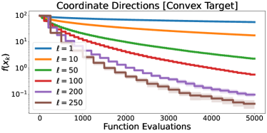
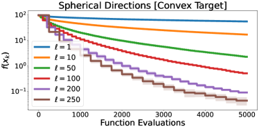
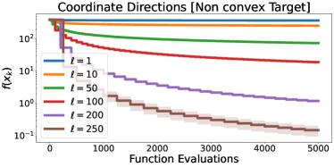
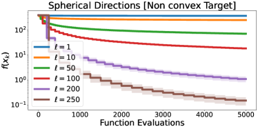
Figure 1: From left to right, function values per function evaluation in optimizing the target function using coordinate and spherical directions with different numbers of directions.

In Figure 1, we show the objective function values, which are available in this controlled setting after each function evaluation. When $l>1$, values are repeated $l$ times indicating that we have to perform at least $l+1$ function evaluations to update the objective function value. Note that for a budget large enough, increasing the number of directions $l$, provides better results w.r.t. a single direction. We also observe that taking orthogonal directions on a sphere provides better performances than coordinate directions when $l$ is small. We argue that this may happen since the random choice of a direction on the sphere allows to better explore the domain with respect to random coordinate directions.

Illustrative Experiments

We consider the problem of minimizing functions that satisfy Assumptions 5 and/or 6. Specifically, we consider the optimization of four functions - details in Appendix C. We plot the mean and standard deviation using $10$ repetitions.

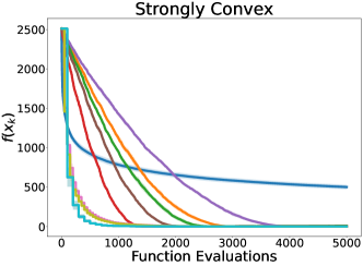
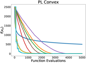
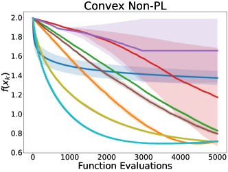
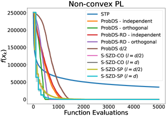
Figure 2: Comparison of different algorithms on a strongly convex, a PL convex, a convex, and a non-convex PL function.

In Figure 2, we plot the objective function values with respect to the number of function evaluations. As we can observe S-SZD obtains the highest performances. While S-SZD performs an update every $l+1$ function evaluations, direct search methods may (or not) need more function evaluations since the step size could be reduced in order to find a descent direction. Looking at the best-performing algorithms, ProbDS and S-SZD, we note that ProbDS with cardinality of the pooling set equal to $d/2$ will perform $d/2$ function evaluation only in worst-case iterations while S-SZD with $l=d/2$ always performs $d/2+1$ function evaluations, however, S-SZD provides better performances in terms of function values decrease. Moreover, note that Direct search algorithms may perform more function evaluations than the cardinality of the pooling set (for instance when the step size is high and there is no descent direction in the pooling set). Thus, ProbDS $d/2$ potentially can perform more than $d/2+1$ function evaluation to perform a single update while S-SZO guarantees to perform no more than $l+1$ function evaluations. Moreover, we note by visual inspection that S-SZD is more stable than ProbDS.

Falkon Tuning

In this section, we consider the problem of parameter tuning for the large-scale kernel method Falkon [50]. Falkon is based on a Nyström approximation of kernel ridge regression. In these experiments, the goal is to minimize the hold-out cross-validation error with respect to two classes of parameters: the length-scale parameters of the Gaussian kernel $\sigma_{1},\cdots,\sigma_{d}$, in each of the $d$ input dimensions; the regularization parameter $\lambda$. We report mean and standard deviation using $5$ repetitions. See additional details in Appendix C.2.

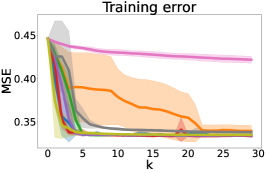
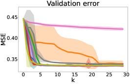
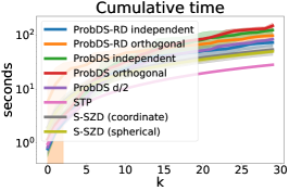
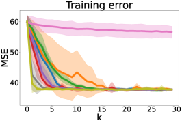
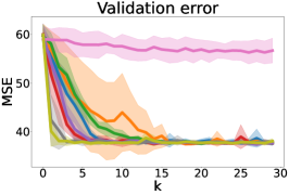
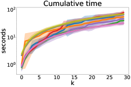
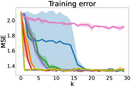
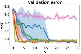
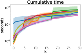
Figure 3: From left to right, training error, validation error and cumulative time obtained by tuning FALKON with different optimizers. From top to bottom, results for HTRU2, CASP and California Housing datasets

From Figure 3, we observe that Algorithm 1 provides the best performances considering both validation error and cumulative time. Despite the iterations of STP are cheaper (it performs 3 function evaluations per iteration, while S-SZD needs $\ell+1>3$ function evaluations per iteration), STP does not perform well on the validation error. Comparing S-SZD with the other algorithms (STP excluded), we see that it achieves the best performances almost always. The test error obtained with Falkon tuned with S-SZD is similar to the best result of other methods - see also Table 3. To conclude, our algorithm outperforms direct search methods in simulated experiments (where assumptions are satisfied) and behaves similarly when assumptions are not satisfied (i.e. in parameter tuning experiments).

5 Conclusion

We presented and analyzed S-SZD, a stochastic zeroth order algorithm for smooth minimization. We derived convergence rates for smooth convex functions and nonconvex functions, under the Polyak-Łojasiewicz assumption. We empirically compared our algorithm with a variety of zeroth order methods, and the numerical results suggest that our algorithm outperforms direct search methods when the assumptions needed for convergence are satisfied. In addition, our algorithm works well also on practical parameter tuning experiments. Our work opens a number of possible research directions. In particular, an interesting question could be the development of an adaptive strategy to choose the direction matrices along the iterations.

Appendix A Auxiliary Results

In this appendix, we provide the preliminary results used to prove the main theorems. Here $z_{k}$ is a realization of $Z_{k}$, $D_{k}F_{k}=D_{(P_{k},h_{k})}F(x_{k},z_{k})$ and $F_{k}=F(x_{k},z_{k})$. We denote by $\mathcal{G}_{k}$ be the filtration $\sigma(P_{1},\cdots,P_{k-1})$ and $\mathcal{F}_{k}$ the filtration $\sigma(Z_{1},\ldots,Z_{k-1})$. The next proposition is a direct consequence of Assumption 1.

Proposition 1.

Let $P_{k}\in\mathbb{R}^{d\times l}$ a direction matrix satisfying Assumption 1 and let $v\in\mathbb{R}^{l}$ and let $w\in\mathbb{R}^{d}$. Then,

$$\|P_{k}v\|^{2}\stackrel{{\scriptstyle\text{a.s.}}}{{=}}\frac{d}{l}\left\lVert{v}\right\rVert^{2}\quad\text{and}\quad\operatorname{\mathbb{E}}[\left\lVert{P_{k}^{\intercal}w}\right\rVert^{2}|\mathcal{G}_{k}]=\left\lVert{w}\right\rVert^{2}.$$

Next we bound the error between our surrogate and the stochastic gradient.

Lemma 1 (Bound on error norm).

Let $z\in\mathcal{Z}$, $F$ a function satisfying Assumption 2 and $P$ a matrix satisfying Assumption 1. Then, $\forall x\in\mathbb{R}^{d}$,

$$\left\lVert{D_{(P,h)}F(x,z)-P^{\intercal}\nabla F(x,z)}\right\rVert\stackrel{{\scriptstyle\text{a.s}}}{{\leq}}\frac{\lambda dh}{2\sqrt{l}}.$$

Proof.

By the definition of the norm, for every $x\in\mathbb{R}^{d}$, and for every $z\in\mathcal{Z}$

$$\left\lVert{D_{(P,h)}F(x,z)-P^{\intercal}\nabla F(x,z)}\right\rVert\stackrel{{\scriptstyle\text{a.s}}}{{=}}\sqrt{\sum\limits_{i=1}^{l}\Big{(}[D_{(P,h)}F(x,z)]_{i}-\left\langle{\nabla F(x,z)},{p^{(i)}}\right\rangle\Big{)}^{2}}.$$ (6)

By the Descent Lemma [43], we have that

$$\Big{|}F(x+hp^{(i)},z)-F(x,z)-h\left\langle{\nabla F(x,z)},{p^{(i)}}\right\rangle\Big{|}\stackrel{{\scriptstyle\text{a.s}}}{{\leq}}\frac{\lambda h^{2}}{2}\left\lVert{p^{(i)}}\right\rVert^{2}.$$

Assumption 1 implies

$$\Big{|}[D_{(P,h)}F(x,z)]_{i}-\left\langle{\nabla F(x,z)},{p^{(i)}}\right\rangle\Big{|}\stackrel{{\scriptstyle\text{a.s}}}{{\leq}}\frac{\lambda hd}{2l}.$$

Using this inequality in equation (6), we get the claim. ∎

The above lemma states that the distance between the finite difference approximations and the directional derivatives is bounded and goes to $0$ when $h\rightarrow 0$. In the next lemma, we show a bound related to the function value decrease along the iterations.

Lemma 2 (Function decrease).

Assume 1, 3, 4. Let the random sequence $(x_{k})$ be generated by Algorithm 1. Then, for every $k\in\mathbb{N}$,

$$\operatorname{\mathbb{E}}_{Z}[\operatorname{\mathbb{E}}_{P}[f_{k+1}|\mathcal{G}_{k}]|\mathcal{F}_{k}]-f_{k} \leq-\frac{\alpha_{k}}{2}\left\lVert{\nabla f_{k}}\right\rVert^{2}+\Big{(}\frac{1}{2}+\frac{\lambda\alpha_{k}d}{l}\Big{)}\Big{(}\frac{\lambda d}{2\sqrt{l}}\Big{)}^{2}\alpha_{k}h_{k}^{2}+\frac{\lambda dG}{2l}\alpha_{k}^{2}.$$

Proof.

Let $f_{k}=\operatorname{\mathbb{E}}_{Z}[F(x_{k},Z)]$. Note that, as $x_{k}$ depends on $z_{1},\cdots,z_{k-1}$, $f_{k}$ is a random variable. By the Descent Lemma, equation (3) and Proposition 1 we have

$$f_{k+1}-f_{k} \leq\left\langle{\nabla f_{k}},{x_{k+1}-x_{k}}\right\rangle+\frac{\lambda}{2}\left\lVert{x_{k+1}-x_{k}}\right\rVert^{2}$$

$$\leq\underbrace{-\alpha_{k}\left\langle{P_{k}^{\intercal}\nabla f_{k}},{D_{k}F_{k}}\right\rangle}_{\textbf{=:a}}+\underbrace{\frac{\lambda d}{2l}\alpha_{k}^{2}\left\lVert{D_{k}F_{k}}\right\rVert^{2}}_{\textbf{=:b}}.$$

Bound on a

Denote $e_{k}:=D_{k}F_{k}-P_{k}^{\intercal}\nabla F_{k}$. Thus

$$-\alpha_{k}\left\langle{P_{k}^{\intercal}\nabla f_{k}},{D_{k}F_{k}}\right\rangle =-\alpha_{k}\left\langle{P_{k}^{\intercal}\nabla f_{k}},{e_{k}}\right\rangle-\alpha_{k}\left\langle{P_{k}^{\intercal}\nabla f_{k}},{P_{k}^{\intercal}\nabla F_{k}}\right\rangle.$$

Bound on b

Adding and subtracting $P_{k}^{\intercal}\nabla F_{k}$ and using Lemma 1, we have

$$\frac{\lambda d}{2l}\alpha_{k}^{2}\left\lVert{D_{k}F_{k}-P_{k}^{\intercal}\nabla F_{k}+P_{k}^{\intercal}\nabla F_{k}}\right\rVert^{2} \leq\frac{\lambda d}{2l}\Big{(}\frac{\lambda d}{2\sqrt{l}}\Big{)}^{2}\alpha_{k}^{2}h_{k}^{2}+\frac{\lambda d}{2l}\alpha_{k}^{2}\left\lVert{P_{k}^{\intercal}\nabla F_{k}}\right\rVert^{2}$$

$$+\frac{\lambda d}{l}\alpha_{k}^{2}\left\langle{e_{k}},{P_{k}^{\intercal}\nabla F_{k}}\right\rangle.$$

Combining the previous bounds, since

$$\left\langle{e_{k}},{P_{k}^{\intercal}\nabla F_{k}}\right\rangle=\left\langle{e_{k}},{P_{k}^{\intercal}\nabla F_{k}-P_{k}^{\intercal}\nabla f_{k}}\right\rangle+\left\langle{e_{k}},{P_{k}^{\intercal}\nabla f_{k}}\right\rangle,$$

we have

$$f_{k+1}-f_{k} \leq\alpha_{k}\Big{(}\frac{\lambda d}{l}\alpha_{k}-1\Big{)}\left\langle{P_{k}^{\intercal}\nabla f_{k}},{e_{k}}\right\rangle-\alpha_{k}\left\langle{P_{k}^{\intercal}\nabla f_{k}},{P_{k}^{\intercal}\nabla F_{k}}\right\rangle+\frac{\lambda d}{2l}\Big{(}\frac{\lambda d}{2\sqrt{l}}\Big{)}^{2}\alpha_{k}^{2}h_{k}^{2}$$

$$+\frac{\lambda d}{2l}\alpha_{k}^{2}\left\lVert{P_{k}^{\intercal}\nabla F_{k}}\right\rVert^{2}+\frac{\lambda d}{l}\alpha_{k}^{2}\left\langle{e_{k}},{P_{k}^{\intercal}\nabla F_{k}-P_{k}^{\intercal}\nabla f_{k}}\right\rangle.$$

By Cauchy-Schwartz inequality and Lemma 1, we get

$$f_{k+1}-f_{k} \leq\alpha_{k}\Big{(}\frac{\lambda d}{l}\alpha_{k}-1\Big{)}\left\langle{P_{k}^{\intercal}\nabla f_{k}},{e_{k}}\right\rangle-\alpha_{k}\left\langle{P_{k}^{\intercal}\nabla f_{k}},{P_{k}^{\intercal}\nabla F_{k}}\right\rangle$$

$$\quad+\frac{\lambda d}{2l}\Big{(}\frac{\lambda d}{2\sqrt{l}}\Big{)}^{2}\alpha_{k}^{2}h_{k}^{2}+\frac{\lambda d}{2l}\alpha_{k}^{2}\left\lVert{P_{k}^{\intercal}\nabla F_{k}}\right\rVert^{2}$$

$$\quad+\frac{\lambda d}{l}\Big{(}\frac{\lambda d}{2\sqrt{l}}\Big{)}\alpha_{k}^{2}h_{k}\left\lVert{P_{k}^{\intercal}(\nabla F_{k}-\nabla f_{k})}\right\rVert.$$

From Young’s inequality we derive that $\left\langle{P_{k}^{\intercal}\nabla f_{k}},{e_{k}}\right\rangle\leq\frac{1}{2}\|P_{k}^{T}\nabla f_{k}\|^{2}+\frac{1}{2}\Big{(}\frac{\lambda d}{2\sqrt{l}}\Big{)}^{2}h_{k}^{2}$ and $h_{k}\|P_{k}^{T}(\nabla F_{k}-\nabla f_{k})\|\leq\frac{h_{k}^{2}}{2}+\frac{1}{2}\|P_{k}^{T}(\nabla F_{k}-\nabla f_{k})\|^{2}$, therefore, taking into account that $\alpha_{k}<l/(\lambda d)$:

$$f_{k+1}-f_{k} \leq\frac{\alpha_{k}}{2}\Big{(}1-\frac{\lambda d}{l}\alpha_{k}\Big{)}\left\lVert{P_{k}^{\intercal}\nabla f_{k}}\right\rVert^{2}+\frac{\alpha_{k}}{2}\Big{(}1-\frac{\lambda d}{l}\alpha_{k}\Big{)}\Big{(}\frac{\lambda d}{2\sqrt{l}}\Big{)}^{2}h_{k}^{2}$$

$$-\alpha_{k}\left\langle{P_{k}^{\intercal}\nabla f_{k}},{P_{k}^{\intercal}\nabla F_{k}}\right\rangle+\frac{\lambda d}{2l}\Big{(}\frac{\lambda d}{2\sqrt{l}}\Big{)}^{2}\alpha_{k}^{2}h_{k}^{2}+\frac{\lambda d}{2l}\alpha_{k}^{2}\left\lVert{P_{k}^{\intercal}\nabla F_{k}}\right\rVert^{2}$$

$$+\frac{\lambda d}{2l}\Big{(}\frac{\lambda d}{2\sqrt{l}}\Big{)}^{2}\alpha_{k}^{2}h_{k}^{2}+\frac{\lambda d}{2l}\alpha_{k}^{2}\left\lVert{P_{k}^{\intercal}(\nabla F_{k}-\nabla f_{k})}\right\rVert^{2}.$$

Observe that $\left\langle{P_{k}^{\intercal}\nabla f_{k}},{P_{k}^{\intercal}\nabla F_{k}}\right\rangle=\left\langle{P_{k}P_{k}^{\intercal}\nabla f_{k}},{\nabla F_{k}}\right\rangle$. Taking the conditional expectation with respect to $\mathcal{G}_{k}$, Proposition 1 implies

$$\operatorname{\mathbb{E}}_{P}[f_{k+1}|\mathcal{G}_{k}]-f_{k} \leq\frac{\alpha_{k}}{2}\Big{(}1-\frac{\lambda d}{l}\alpha_{k}\Big{)}\left\lVert{\nabla f_{k}}\right\rVert^{2}+\frac{\alpha_{k}}{2}\Big{(}1-\frac{\lambda d}{l}\alpha_{k}\Big{)}\Big{(}\frac{\lambda d}{2\sqrt{l}}\Big{)}^{2}h_{k}^{2}$$

$$-\alpha_{k}\left\langle{\nabla f_{k}},{\nabla F_{k}}\right\rangle+\frac{\lambda d}{2l}\Big{(}\frac{\lambda d}{2\sqrt{l}}\Big{)}^{2}\alpha_{k}^{2}h_{k}^{2}+\frac{\lambda d}{2l}\alpha_{k}^{2}\left\lVert{\nabla F_{k}}\right\rVert^{2}$$

$$+\frac{\lambda d}{2l}\Big{(}\frac{\lambda d}{2\sqrt{l}}\Big{)}^{2}\alpha_{k}^{2}h_{k}^{2}+\frac{\lambda d}{2l}\alpha_{k}^{2}\left\lVert{\nabla F_{k}-\nabla f_{k}}\right\rVert^{2}.$$

Note that $\|\nabla F_{k}\|^{2}=\|\nabla F_{k}-\nabla f_{k}\|^{2}+\|\nabla f_{k}\|^{2}+2\left\langle{\nabla F_{k}-\nabla f_{k}},{\nabla f_{k}}\right\rangle$. Taking the conditional expectation with respect to the filtration $\mathcal{F}_{k}$, we get

$$\operatorname{\mathbb{E}}_{Z}[\operatorname{\mathbb{E}}_{P}[f_{k+1}|\mathcal{G}_{k}]|\mathcal{F}_{k}]-f_{k} \leq\frac{\alpha_{k}}{2}\Big{(}1-\frac{\lambda d}{l}\alpha_{k}\Big{)}\left\lVert{\nabla f_{k}}\right\rVert^{2}+\frac{\alpha_{k}}{2}\Big{(}1-\frac{\lambda d}{l}\alpha_{k}\Big{)}\Big{(}\frac{\lambda d}{2\sqrt{l}}\Big{)}^{2}h_{k}^{2}$$

$$-\alpha_{k}\left\lVert{\nabla f_{k}}\right\rVert^{2}+\frac{\lambda d}{2l}\Big{(}\frac{\lambda d}{2\sqrt{l}}\Big{)}^{2}\alpha_{k}^{2}h_{k}^{2}+\frac{\lambda Gd}{2l}\alpha_{k}^{2}$$

$$+\frac{\lambda d}{2l}\alpha_{k}^{2}\left\lVert{\nabla f_{k}}\right\rVert^{2}+\frac{\lambda d}{2l}\Big{(}\frac{\lambda d}{2\sqrt{l}}\Big{)}^{2}\alpha_{k}^{2}h_{k}^{2}+\frac{\lambda Gd}{2l}\alpha_{k}^{2}.$$

Rearrangin the terms, we get the claim. ∎ Note that both Lemma 1 and Lemma 2 hold also for non-convex functions. In the next appendix, we provide preliminary results for the convex case.

A.1 Preliminary results: Convex case

We start studying the convergence properties of Algorithm 1 by a fundamental energy estimate.

Lemma 3 (Convergence).

Under Assumptions 1,2,3,5, let $(x_{k})$ be the random sequence generated by Algorithm 1. Define, for every $k\in\mathbb{N}$,

$$C_{k}=\frac{\lambda^{2}d^{3}}{2l^{2}}\alpha_{k}^{2}h_{k}^{2}+\frac{2dG}{l}\alpha_{k}^{2}\quad\text{and}\quad\rho_{k}=\frac{\lambda d\sqrt{d}}{l}\alpha_{k}h_{k}.$$ (7)

Let $\bar{x}\in\operatornamewithlimits{arg\,min}f$ and let $u_{k}=\left\lVert{x_{k}-\bar{x}}\right\rVert$. Then, for every $k\in\mathbb{N}$,

$$\operatorname{\mathbb{E}}_{Z}[\operatorname{\mathbb{E}}_{P}[u_{k+1}^{2}|\mathcal{G}_{k}]|\mathcal{F}_{k}]-u_{k}^{2} \leq C_{k}+\frac{2d}{l}\alpha_{k}^{2}\left\lVert{\nabla f_{k}}\right\rVert^{2}+2\alpha_{k}\left\langle{\nabla f_{k}},{\bar{x}-x_{k}}\right\rangle+\rho_{k}u_{k}.$$ (8)

Moreover, under Assumption 4, the sequence $\left\lVert{x_{k}-\bar{x}}\right\rVert$ is a.s. convergent,

$$\alpha_{k}\left\lVert{\nabla f_{k}}\right\rVert^{2}\in\ell^{1},\qquad\alpha_{k}(f_{k}-\min f)\in\ell^{1},\qquad\liminf\limits_{k}f_{k}\stackrel{{\scriptstyle\text{a.s.}}}{{=}}\min f.$$

and there exists $x^{*}\in\operatornamewithlimits{arg\,min}f$ such that $x_{k}\rightarrow x^{*}$ a.s.

Proof.

Let, $\bar{x}\in\operatornamewithlimits{arg\,min}f$. Using the definition of $x_{k+1}$ in Algorithm 1 we derive

$$\left\lVert{x_{k+1}-\bar{x}}\right\rVert^{2}-\left\lVert{x_{k}-\bar{x}}\right\rVert^{2}=\underbrace{\alpha_{k}^{2}\left\lVert{P_{k}D_{k}F_{k}}\right\rVert^{2}}_{\text{\bf=:a}}+\underbrace{2\alpha_{k}\left\langle{P_{k}D_{k}F_{k}},{\bar{x}-x_{k}}\right\rangle}_{\text{\bf=:b}}.$$

Denoting with $e_{k}:=D_{k}F_{k}-P_{k}^{\intercal}\nabla F_{k}$, we bound separately the two terms. To bound a, we use Proposition 1 and we add and subtract $P_{k}^{\intercal}\nabla F_{k}$, to obtain

$$\left\lVert{P_{k}D_{k}F_{k}}\right\rVert^{2}\stackrel{{\scriptstyle\text{a.s.}}}{{=}}\frac{d}{l}\left\lVert{D_{k}F_{k}-P_{k}^{\intercal}\nabla F_{k}+P_{k}^{\intercal}\nabla F_{k}}\right\rVert^{2}\leq\frac{2d}{l}\left\lVert{e_{k}}\right\rVert^{2}+\frac{2d}{l}\left\lVert{P_{k}^{\intercal}\nabla F_{k}}\right\rVert^{2}.$$

Moreover, it follows from Lemma 1 that $\left\lVert{e_{k}}\right\rVert^{2}\leq({\lambda d}/{2\sqrt{l}})^{2}\alpha_{k}^{2}h_{k}^{2}$. To bound b, we add and subtract $P_{k}P_{k}^{\intercal}\nabla F_{k}$ and we derive

$$2\alpha_{k}\left\langle{P_{k}D_{k}F_{k}},{\bar{x}-x_{k}}\right\rangle =2\alpha_{k}\left\langle{P_{k}P_{k}^{\intercal}\nabla F_{k}},{\bar{x}-x_{k}}\right\rangle+2\alpha_{k}\left\langle{P_{k}e_{k}},{\bar{x}-x_{k}}\right\rangle$$

$$\leq 2\alpha_{k}\left\langle{P_{k}P_{k}^{\intercal}\nabla F_{k}},{\bar{x}-x_{k}}\right\rangle+2\sqrt{\frac{d}{l}}\Big{(}\frac{\lambda d}{2\sqrt{l}}\Big{)}\alpha_{k}h_{k}\left\lVert{\bar{x}-x_{k}}\right\rVert,$$

where in the last inequality we used Cauchy-Schwartz, Proposition 1 and Lemma 1. Using the upper-bounds above, we have

$$u_{k+1}^{2}-u_{k}^{2} \leq\frac{2d}{l}\Bigg{(}\frac{\lambda d}{2\sqrt{l}}\Bigg{)}^{2}\alpha_{k}^{2}h_{k}^{2}+\frac{2d}{l}\alpha_{k}^{2}\left\lVert{P_{k}^{\intercal}\nabla F_{k}}\right\rVert^{2}+2\alpha_{k}\left\langle{P_{k}P_{k}^{\intercal}\nabla F_{k}},{\bar{x}-x_{k}}\right\rangle+2\sqrt{\frac{d}{l}}\Big{(}\frac{\lambda d}{2\sqrt{l}}\Big{)}\alpha_{k}h_{k}u_{k}.$$

Taking the conditional expectation with respect to $\mathcal{G}_{k}$, and using Proposition 1,

$$\operatorname{\mathbb{E}}_{P}[u_{k+1}^{2}|\mathcal{G}_{k}]-u_{k}^{2} \leq\frac{2d}{l}\Bigg{(}\frac{\lambda d}{2\sqrt{l}}\Bigg{)}^{2}\alpha_{k}^{2}h_{k}^{2}+\frac{2d}{l}\alpha_{k}^{2}\left\lVert{\nabla F_{k}}\right\rVert^{2}+2\alpha_{k}\left\langle{\nabla F_{k}},{\bar{x}-x_{k}}\right\rangle+2\sqrt{\frac{d}{l}}\Big{(}\frac{\lambda d}{2\sqrt{l}}\Big{)}\alpha_{k}h_{k}u_{k}.$$

Adding and subtracting $\nabla f_{k}$ in the term $\left\lVert{\nabla F_{k}}\right\rVert^{2}$, we get

$$\operatorname{\mathbb{E}}_{P}[u_{k+1}^{2}|\mathcal{G}_{k}]-u_{k}^{2} \leq\frac{2d}{l}\Bigg{(}\frac{\lambda d}{2\sqrt{l}}\Bigg{)}^{2}\alpha_{k}^{2}h_{k}^{2}+\frac{2d}{l}\alpha_{k}^{2}\left\lVert{\nabla F_{k}-\nabla f_{k}}\right\rVert^{2}+\frac{2d}{l}\alpha_{k}^{2}\left\lVert{\nabla f_{k}}\right\rVert^{2}$$

$$+\frac{4d}{l}\alpha_{k}^{2}\left\langle{\nabla F_{k}-\nabla f_{k}},{\nabla f_{k}}\right\rangle+2\alpha_{k}\left\langle{\nabla F_{k}},{x^{*}-x_{k}}\right\rangle$$

$$+2\sqrt{\frac{d}{l}}\Big{(}\frac{\lambda d}{2\sqrt{l}}\Big{)}\alpha_{k}h_{k}u_{k}.$$

Define $C_{k}$ and $\rho_{k}$ as in (7). Taking the conditional expectation, by Lemma 1, we derive equation (8). In order to prove the second part of the statement, we apply Fubini’s Theorem and Young’s inequality with parameter $\tau_{k}$ in (8). We get

$$\operatorname{\mathbb{E}}_{P}[\operatorname{\mathbb{E}}_{Z}[u_{k+1}^{2}|\mathcal{F}_{k}]|\mathcal{G}_{k}]-u_{k}^{2} \leq C_{k}+\frac{2d}{l}\alpha_{k}^{2}\left\lVert{\nabla f_{k}}\right\rVert^{2}+2\alpha_{k}\left\langle{\nabla f_{k}},{\bar{x}-x_{k}}\right\rangle$$

$$+\frac{1}{2\tau_{k}}\Big{(}\frac{\lambda d\sqrt{d}}{l}\Big{)}^{2}\alpha_{k}^{2}h_{k}^{2}+\frac{\tau_{k}}{2}u_{k}^{2}.$$

Next we set $\tau_{k}=({d\sqrt{d}}/{l})\alpha_{k}h_{k}$, $\tilde{C}_{k}=({d}/{l})\alpha_{k}\Big{(}({\lambda^{2}d^{2}}/({2l}))\alpha_{k}h_{k}^{2}+2G\alpha_{k}+{\lambda^{2}\sqrt{d}}/{2}h_{k}\Big{)}$ and $\tilde{\rho}_{k}=({d\sqrt{d}}/({2l}))\alpha_{k}h_{k}$. Rearranging the terms, we get

$$\operatorname{\mathbb{E}}_{P}[\operatorname{\mathbb{E}}_{Z}[u_{k+1}^{2}|\mathcal{F}_{k}]|\mathcal{G}_{k}]-(1+\tilde{\rho}_{k})u_{k}^{2} \leq\tilde{C}_{k}+\frac{2d}{l}\alpha_{k}^{2}\left\lVert{\nabla f_{k}}\right\rVert^{2}+2\alpha_{k}\left\langle{\nabla f_{k}},{\bar{x}-x_{k}}\right\rangle.$$ (9)

Baillon-Haddad Theorem [2] and Assumption 4 yield,

$$\operatorname{\mathbb{E}}_{P}[\operatorname{\mathbb{E}}_{Z}[u_{k+1}^{2}|\mathcal{F}_{k}]|\mathcal{G}_{k}]-(1+\tilde{\rho}_{k})u_{k}^{2} \leq\tilde{C}_{k}-2\Big{(}\frac{1}{\lambda}-\frac{\bar{\alpha}d}{l}\Big{)}\alpha_{k}\left\lVert{\nabla f_{k}}\right\rVert^{2}.$$

Thus,

$$\operatorname{\mathbb{E}}_{P}[\operatorname{\mathbb{E}}_{Z}[u_{k+1}^{2}|\mathcal{F}_{k}]|\mathcal{G}_{k}]-(1+\tilde{\rho}_{k})u_{k}^{2}+2\Big{(}\frac{1}{\lambda}-\frac{\bar{\alpha}d}{l}\Big{)}\alpha_{k}\left\lVert{\nabla f_{k}}\right\rVert^{2} \leq\tilde{C}_{k}.$$

Note that $(\frac{1}{\lambda}-\frac{\bar{\alpha}d}{l})>0$. By Assumption 4, $\tilde{C}_{k}$ and $\tilde{\rho}_{k}$ belong to $\ell^{1}$. Denoting with $\mathcal{H}_{k}=\sigma(P_{1},Z_{1},\cdots,P_{k-1},Z_{k-1})$, by Fubini’s Theorem, we have

$$\operatorname{\mathbb{E}}_{P}[\operatorname{\mathbb{E}}_{Z}[u_{k+1}^{2}|\mathcal{F}_{k}]|\mathcal{G}_{k}]=\operatorname{\mathbb{E}}_{(P,Z)}[u_{k+1}^{2}|\mathcal{H}_{k}].$$

Then Robbins-Siegmund Theorem [47] implies that the sequence $u_{k}=\left\lVert{x_{k}-\bar{x}}\right\rVert$ is a.s. convergent and that a.s. $\alpha_{k}\left\lVert{\nabla f_{k}}\right\rVert^{2}\in\ell^{1}$. Since $f$ is convex, we derive from equation (9) that

$$\operatorname{\mathbb{E}}_{(P,Z)}[u_{k+1}^{2}|\mathcal{H}_{k}]-(1+\tilde{\rho}_{k})u_{k}^{2}+2\alpha_{k}(f_{k}-f^{*}) \leq\tilde{C}_{k}+\frac{2d}{l}\alpha_{k}^{2}\left\lVert{\nabla f_{k}}\right\rVert^{2}.$$

Since $\alpha_{k}^{2}\left\lVert{\nabla f_{k}}\right\rVert^{2}\in\ell^{1}$, again by Robbins-Siegmund Theorem, we conclude that a.s. $\alpha_{k}(f_{k}-\min f)\in\ell^{1}.$ By Assumption 4, the sequence $\alpha_{k}$ does not belong to $\ell^{1}$, so that the previous result implies

$$\liminf\limits_{k}f_{k}\stackrel{{\scriptstyle\text{a.s.}}}{{=}}\min f.$$ (10)

Now consider Lemma 2. Recalling that $\alpha_{k}\left\lVert{\nabla f_{k}}\right\rVert^{2}\in\ell^{1}$ and Assumption 4, we know that $\operatorname{\mathbb{E}}_{(P,Z)}[f_{k+1}|\mathcal{H}_{k}]-f_{k}$ is bounded by a sequence belonging to $\ell^{1}$. Then, using Robbins-Siegmund Theorem, we know that a.s. there exists the limit of $f_{k}$ for $k\to+\infty$. Then, combining with Eq. (10), we have that $\lim\limits_{k}f_{k}\stackrel{{\scriptstyle\text{a.s.}}}{{=}}\min f.$ In particular, every a.s. cluster point of the sequence $(x_{k})$ is a.s. a minimizer of the function $f$. Recall also that $\left\lVert{x_{k}-x^{*}}\right\rVert$ is a.s. convergent for every $x^{*}\in\operatornamewithlimits{arg\,min}f$. Then, by Opial’s Lemma, there exists $x^{*}\in\operatornamewithlimits{arg\,min}f$ such that $x_{k}\rightarrow x^{*}$ a.s. ∎

Lemma 4 is the extension to the stochastic setting of [33, Lemma 5.1]. The difference between equation (8) and [33, Lemma 5.1] is the presence of an extra term containing $G$ and related to the stochastic information. Now, to get convergence rates from the previous energy estimation, we need to upper bound the two quantities $\sqrt{\operatorname{\mathbb{E}}[\left\lVert{x_{k}-x^{*}}\right\rVert^{2}]}$ and $\sum\limits_{j=0}^{k}\alpha_{j}\operatorname{\mathbb{E}}[\left\lVert{\nabla f_{j}}\right\rVert^{2}]$.

Lemma 4.

Let Assumptions 1, 2, 3, 4 and 5 hold and $(x_{k})$ be the random sequence generated by Algorithm 1. Then, for each $k\in\mathbb{N}$ and any minimizer $x^{*}$ of $f$

$$\sqrt{\operatorname{\mathbb{E}}[\left\lVert{x_{k}-x^{*}}\right\rVert^{2}]}\leq\sqrt{S_{k-1}}+\sum\limits_{j=0}^{k}\rho_{j},$$ (11)

where

$$S_{k}=\operatorname{\mathbb{E}}[\left\lVert{x_{0}-x^{*}}\right\rVert^{2}]+\sum\limits_{j=0}^{k}\frac{d}{l}\Bigg{(}\frac{\lambda^{2}d^{2}}{2l}h_{j}^{2}+2G\Bigg{)}\alpha_{j}^{2}\qquad\text{and}\qquad\rho_{k}:=\frac{d\sqrt{d}}{2l}\alpha_{k}h_{k}.$$ (12)

Denoting with $\Delta=\Big{(}\frac{1}{\lambda}-\frac{\bar{\alpha}d}{l}\Big{)}$, we have that, for all $k\in\mathbb{N}$ and any minimizer of $f$

$$\sum\limits_{j=0}^{k}\alpha_{j}\operatorname{\mathbb{E}}[\left\lVert{\nabla f_{j}}\right\rVert^{2}]\leq\frac{1}{2\Delta}\Big{(}S_{k}+\sum\limits_{j=0}^{k}\rho_{j}\sqrt{\operatorname{\mathbb{E}}[\left\lVert{x_{j}-x^{*}}\right\rVert^{2}]}\Big{)}.$$ (13)

Proof.

Let $C_{k}=\frac{d}{l}\Big{(}\frac{\lambda^{2}d^{2}}{2l}h_{k}^{2}+2G\Big{)}\alpha_{k}^{2}$. The Baillon-Haddad Theorem applied in equation (8) implies

$$\operatorname{\mathbb{E}}_{P}[\operatorname{\mathbb{E}}_{Z}[\left\lVert{x_{k+1}-x^{*}}\right\rVert^{2}|\mathcal{F}_{k}]|\mathcal{G}_{k}]-\left\lVert{x_{k}-x^{*}}\right\rVert^{2} \leq C_{k}-2\alpha_{k}\Delta\left\lVert{\nabla f_{k}}\right\rVert^{2}+\rho_{k}\left\lVert{x^{*}-x_{k}}\right\rVert.$$

Taking the total expectation and letting $u_{k}:=\sqrt{\operatorname{\mathbb{E}}[\left\lVert{x_{k+1}-x^{*}}\right\rVert^{2}]}$, we get

$$u_{k+1}^{2}-u_{k}^{2}\leq C_{k}-2\alpha_{k}\Delta\operatorname{\mathbb{E}}[\left\lVert{\nabla f_{k}}\right\rVert^{2}]+\rho_{k}u_{k}.$$

Summing the previous inequality from $0$ to $k$ we derive

$$u_{k+1}^{2}+2\Delta\sum\limits_{j=0}^{k}\alpha_{j}\operatorname{\mathbb{E}}[\left\lVert{\nabla f_{j}}\right\rVert^{2}]\leq S_{k}+\sum\limits_{j=0}^{k}\rho_{j}u_{j},$$

from which we obtain equation (12). To derive (11), we observe that $\rho_{k}$ is non-negative, $S_{k}$ is non-decreasing and $S_{0}\geq u_{0}^{2}$. Since $u_{k+1}^{2}\leq S_{k}+\sum\limits_{j=0}^{k}\rho_{j}u_{j}$, we conclude by the (discrete) Bihari’s Lemma [33, Lemma 9.8]. ∎

Appendix B Proofs of the main results

In this section, we provide proofs for Theorem 1, Theorem 2, Corollary 1 and Corollary 2.

B.1 Proof of Theorem 1

Let $C_{k}=\frac{d}{l}\Big{(}\frac{\lambda^{2}d^{2}}{2l}h_{k}^{2}+2G\Big{)}\alpha_{k}^{2}$. By Lemma 3

$$\operatorname{\mathbb{E}}_{Z}[\operatorname{\mathbb{E}}_{P}[\left\lVert{x_{k+1}-x^{*}}\right\rVert^{2}|\mathcal{G}_{k}]|\mathcal{F}_{k}]-\left\lVert{x_{k}-x^{*}}\right\rVert^{2} \leq C_{k}+\frac{2d}{l}\alpha_{k}^{2}\left\lVert{\nabla f_{k}}\right\rVert^{2}+2\alpha_{k}\left\langle{\nabla f_{k}},{x^{*}-x_{k}}\right\rangle+\rho_{k}\left\lVert{x^{*}-x_{k}}\right\rVert.$$

Let us denote with $u_{k}=\sqrt{\operatorname{\mathbb{E}}[\left\lVert{x_{k}-x^{*}}\right\rVert^{2}]}$. Taking the total expectation, the convexity of $f$ implies

$$u_{k+1}^{2}-u_{k}^{2}\leq C_{k}+\frac{2d}{l}\alpha_{k}^{2}\operatorname{\mathbb{E}}[\left\lVert{\nabla f_{k}}\right\rVert^{2}]-2\alpha_{k}\operatorname{\mathbb{E}}[(f_{k}-f^{*})]+\rho_{k}u_{k}$$

and therefore

$$u_{k+1}^{2}-u_{k}^{2}+2\alpha_{k}\operatorname{\mathbb{E}}[(f_{k}-f^{*})]\leq C_{k}+\frac{2d}{l}\alpha_{k}^{2}\operatorname{\mathbb{E}}[\left\lVert{\nabla f_{k}}\right\rVert^{2}]+\rho_{k}u_{k}.$$

Summing from $0$ to $k$, we have

$$u_{k+1}^{2}+2\sum\limits_{j=0}^{k}\alpha_{j}\operatorname{\mathbb{E}}[(f_{j}-f^{*})]\leq\underbrace{u_{0}^{2}+\sum\limits_{j=0}^{k}C_{j}}_{=S_{k}}+\sum\limits_{j=0}^{k}\frac{2d}{l}\alpha_{j}^{2}\operatorname{\mathbb{E}}[\left\lVert{\nabla f_{j}}\right\rVert^{2}]+\sum\limits_{j=0}^{k}\rho_{j}u_{j}.$$

Clearly $u_{k}^{2}\geq 0$ and by Assumption 4, $0<\alpha_{k}\leq\bar{\alpha}<\frac{l}{d\lambda}$ for each $k\in\mathbb{N}$. Then,

$$2\sum\limits_{j=0}^{k}\alpha_{j}\operatorname{\mathbb{E}}[(f_{j}-f^{*})]\leq S_{k}+\frac{2\bar{\alpha}d}{l}\sum\limits_{j=0}^{k}\alpha_{j}\operatorname{\mathbb{E}}[\left\lVert{\nabla f_{j}}\right\rVert^{2}]+\sum\limits_{j=0}^{k}\rho_{j}u_{j}.$$

Equations (11) and (12) of Lemma 4 yield

$$2\sum\limits_{j=0}^{k}\alpha_{j}\operatorname{\mathbb{E}}[(f_{j}-f^{*})] \leq S_{k}+\frac{\bar{\alpha}d}{\Delta l}S_{k}+\frac{\bar{\alpha}d}{\Delta l}\sum\limits_{j=0}^{k}\rho_{j}u_{j}+\sum\limits_{j=0}^{k}\rho_{j}u_{j}$$

$$\sum\limits_{j=0}^{k}\alpha_{j}\operatorname{\mathbb{E}}[(f_{j}-f^{*})] \leq\underbrace{\frac{\bar{\alpha}d+\Delta l}{2\Delta l}\Bigg{(}S_{k}+\sum\limits_{j=0}^{k}\rho_{j}\Bigg{(}\sqrt{S_{j-1}}+\sum\limits_{i=0}^{j}\rho_{i}\Bigg{)}\Bigg{)}}_{=D_{k}}.$$

As $S_{k},\rho_{k}$ and $C_{k}$ are in $\ell^{1}$, we have that $D_{k}\leq C<\infty$. Moreover, by convexity,

$$\operatorname{\mathbb{E}}[f(\bar{x}_{k})-\min f]\leq\frac{\sum\limits_{j=0}^{k}\alpha_{j}\operatorname{\mathbb{E}}[f(x_{j})-\min f]}{\sum\limits_{j=0}^{k}\alpha_{j}},$$

which concludes the proof.

B.2 Proof of Corollary 1

From Theorem 1, we have

$$\operatorname{\mathbb{E}}[f(\bar{x}_{k})-\min f]\leq{C_{k}}/\Big{(}{\sum\limits_{i=0}^{k}\alpha_{i}}\Big{)},$$ (14)

where $C_{k}=\frac{l\Delta+d\bar{\alpha}}{2l\Delta}\Big{(}S_{k}+\sum\limits_{j=0}^{k}\rho_{j}\Big{(}\sqrt{S_{j}}+\sum\limits_{i=0}^{j}\rho_{i}\Big{)}\Big{)}$ with $\rho_{k}=\alpha_{k}\frac{\lambda h_{k}d\sqrt{d}}{l}$ and

$$S_{k} =\left\lVert{x_{0}-x^{*}}\right\rVert^{2}+\sum\limits_{j=0}^{k}\frac{d}{l}\Big{(}\frac{\lambda^{2}d^{2}}{2l}h_{j}^{2}+2G\Big{)}\alpha_{j}^{2}.$$

Replacing $\alpha_{k}$ and $h_{k}$ with the sequences above, we have that

$$\rho_{k}=k^{-(c+r)}\frac{\alpha h\lambda d\sqrt{d}}{l}.$$ (15)

Now, we bound the different terms in eq. (14). Let $C_{1}=\frac{\lambda^{2}}{2(1-2c-2r)}$ and $C_{2}=\frac{2G}{1-2c}$. Then,

$$S_{k}\leq\left\lVert{x_{0}-x^{*}}\right\rVert^{2}+C_{1}\frac{\alpha^{2}d^{3}h^{2}}{l^{2}}k^{-2(c+r)+1}+C_{2}\frac{d\alpha^{2}}{l}k^{-2c+1}.$$

Let $\Lambda=d\lambda/l$. Using the bound on $S_{k}$ and equation (15), we have

$$C_{k} \leq\frac{1}{1-\bar{\alpha}\Lambda}\Big{(}\left\lVert{x_{0}-x^{*}}\right\rVert^{2}+C_{1}\frac{\alpha^{2}h^{2}d^{3}}{l^{2}}k^{1-2(c+r)}+C_{2}\frac{\alpha^{2}d}{l}k^{1-2c}$$

$$+C_{3}\frac{\alpha hd\sqrt{d}}{l}\left\lVert{x_{0}-x^{*}}\right\rVert k^{1-c-r}+C_{4}\frac{\alpha^{2}h^{2}d^{3}}{l^{2}}k^{3/2-2c-2r}$$

$$+C_{5}\frac{\alpha^{2}hd^{2}}{l\sqrt{l}}k^{3/2-2c-r}+C_{6}\frac{\alpha^{2}h^{2}d^{3}}{l^{2}}k^{2-2c-2r}\Big{)},$$

where $C_{3}=\frac{\lambda}{1-c-r}$, $C_{4}=\frac{\lambda\sqrt{C_{1}}}{3/2-2c-2r}$,$C_{5}=\frac{\sqrt{C_{2}}\lambda}{3/2-2c-r}$ and $C_{6}=\frac{\lambda^{3}}{(1-c-r)(2-2c-2r)}$. Then, dividing by $\sum\limits_{i=0}^{k}\alpha_{i}$ and taking $\alpha=\frac{1}{2\Lambda}$, we get

$${C_{k}}/\Big{(}{\sum\limits_{i=0}^{k}\alpha_{i}}\Big{)}\leq\frac{d}{l}\frac{C^{\prime}}{k^{1-c}}+o\Big{(}\frac{1}{k^{1-c}}\Big{)}\quad\text{with}\quad C^{\prime}=\frac{2\Lambda\left\lVert{x_{0}-x^{*}}\right\rVert^{2}}{(1-c)}.$$

Recall that each step of the algorithm requires $l+1$ function evaluations. Then, given a tolerance $\epsilon\in(0,1)$, the number of function evaluations to reach the $\epsilon$ tolerance is proportional to

$$(l+1)\Big{(}\frac{d}{l\epsilon}\Big{)}^{\frac{1}{1-c}}.$$

B.3 Proof of Theorem 2

Using Lemma 2 and Assumption 4, we get

$$\operatorname{\mathbb{E}}_{Z}[\operatorname{\mathbb{E}}_{P}[f_{k+1}|\mathcal{G}_{k}]|\mathcal{F}_{k}]-f_{k} \leq-\frac{\alpha_{k}}{2}\left\lVert{\nabla f_{k}}\right\rVert^{2}+C\alpha_{k}h_{k}^{2}+\frac{\lambda Gd}{2l}\alpha_{k}^{2}.$$

Where $C=\Big{(}\frac{1}{2}+\frac{\lambda\bar{\alpha}d}{l}\Big{)}\Big{(}\frac{\lambda d}{2\sqrt{l}}\Big{)}^{2}$. By Assumption 6, we obtain

$$\operatorname{\mathbb{E}}_{Z}[\operatorname{\mathbb{E}}_{P}[f_{k+1}|\mathcal{G}_{k}]|\mathcal{F}_{k}]-f_{k} \leq-\frac{\alpha_{k}}{2}\gamma(f_{k}-f^{*})+C\alpha_{k}h_{k}^{2}+\frac{\lambda Gd}{2l}\alpha_{k}^{2}.$$

Taking the full expectation, we get the claim.

B.4 Proof of Corollary 2

We start by fixing $\alpha_{k}=\alpha/k^{c}$ and $h_{k}=h/k^{c/2}$ with $0<\alpha<l/(d\lambda)$, $h>0$ and $c>0$. By Theorem 2, we get

$$\operatorname{\mathbb{E}}[f(x_{k+1})-\min f] \leq\Big{(}1-\frac{C_{1}\alpha}{k^{c}}\Big{)}\operatorname{\mathbb{E}}[f(x_{k})-\min f]+\frac{\alpha(C_{2}h^{2}+C_{3}\alpha)}{k^{2c}},$$ (16)

where $C_{1}=\gamma/2$, $C_{2}=\Big{(}\frac{1}{2}+\frac{\lambda{\alpha}d}{l}\Big{)}\Big{(}\frac{\lambda d}{2\sqrt{l}}\Big{)}^{2}$ and $C_{3}=\frac{\lambda d}{2l}G$. We conclude the proof by Chung’s Lemma [11].

Appendix C Experiment Details

Here we report details on the experiments performed. We implemented every script in Python3 and used scikit-learn[42], numpy[27] and pytorch[41] libraries.

C.1 Synthetic experiments

In this appendix, we provide details about synthetic experiments presented in Section 4. We performed four experiments on functions that satisfy Assumptions 5 and/or 6. Specifically, we considered a strongly convex, a PL convex, a convex and a PL non-convex function. The dimension of the domain is set to $d=100$ for strongly convex (F1), PL convex (F2), and PL non-convex (F3) targets. In particular, these functions are defined in Table 1.

Table 1: Target function used in synthetic experiments.

Name	Function	Details
F1	$f(x)=1/d\left\lVert{Ax}\right\rVert^{2}$	$A\in\mathbb{R}^{d\times d}$ full rank
F2	$f(x)=1/d\left\lVert{Ax}\right\rVert^{2}$	$A\in\mathbb{R}^{d\times d}$ rank deficient
F3	$f(x)=1/d\left\lVert{Ax}\right\rVert^{2}+3\sin^{2}(c^{\intercal}x)$	$A\in\mathbb{R}^{d\times d}$ and $Ac=c$

Both three functions have $x^{*}=[0,\cdots,0]^{\intercal}\in\operatornamewithlimits{arg\,min}f$. In these experiments, at each time step $k$, Algorithm 1 observes a $z_{k}$ which represents a row of the matrix $A$ (in all the three cases) and performs the iteration described in equation (3). For DS methods, we used the sufficient decrease condition (instead of the simple decrease condition for STP[5]) with forcing function $\rho(\alpha)=\min\{10^{-5},10^{-5}\alpha^{2}\left\lVert{d}\right\rVert^{2}\},$ where $d$ is the direction selected and a sketched direction for ProbDS-RD [48]. The initial step-size is set to $\alpha_{0}=1.0$ and for STP, the step-size is decreased as $\alpha_{k}=\alpha_{0}/(k+1)$. Expansion and contraction factors are set to $2$ and $1/2$ respectively. The maximum step size is set to $5$ for the strongly convex and PL convex functions and to $10$ for non-convex functions. For S-SZD, we set $\alpha_{k}=({l}/{d})*10^{-2}*k^{-(1/2+\delta)}$ and $h_{k}=10^{-8}/\sqrt{k}$ for convex and non-convex functions. While in the first experiment of Section 4, for $\delta=10^{-10}$, we set $\alpha_{k}$ and $h_{k}$ as $5\times 10^{-3}\frac{l}{d}k^{-(1/2+\delta)}$ and $10^{-7}/\sqrt{k}$ respectively.

Convex non-PL case

For the experiment on the convex non-PL function, we generated some synthetic data from two multivariate Gaussian distributions and we optimized a logistic regressor in order to perform classification. Specifically, we generated a synthetic binary classification dataset composed of two classes both of $500$ points in $20$ dimensions. Then, we trained a logistic regressor in order to perform classification. The optimization task involved by logistic regression is then solved using the zeroth order strategies indicated in Section 4. Specifically, at every S-SZD step, we observe a random point of the dataset and compute the surrogate (2) instead of the gradient. We used a step-size $\alpha_{k}=k^{-(1/2+10^{-10})}$ and a discretization $h_{k}=10^{-8}/\sqrt{k}$.

C.2 Falkon tuning experiments details

In this appendix, we describe how datasets are preprocessed, split and how parameters of the optimizers are selected to perform Falkon experiments. As indicated in Section 4, we focus on tuning kernel and regularization parameters. Given a dataset $D=\{(x_{i},y_{i})\}_{i=1}^{n}$ where $y_{i}=f(x_{i})+\epsilon_{i}$, we want to approximate $f$ with a surrogate $f_{w}$ which depends on some parameters $w$. To avoid overfitting, we split the dataset in two, the first part including the data from 1 to $n_{1}$ (training) and the second one including the remaining points (validation). The training part (composed of the $80\%$ of the points) is used to build $f_{w}$. The validation part (composed of the remaining $20\%$ of the points) is used to choose hyperparameters $\lambda$ and $\sigma=(\sigma_{1},\ldots,\sigma_{d})$. Specifically, the problem we want to solve is the following

$$w_{\lambda,\sigma}^{*}\in\operatornamewithlimits{arg\,min}\limits_{w\in W}\sum\limits_{i=1}^{n_{1}}(f_{w}(x_{i},\sigma)-y_{i})^{2}+\lambda\|w\|^{2}$$ (17)

$$(\lambda^{*},\sigma^{*})\in\operatornamewithlimits{arg\,min}\limits_{\lambda\in\mathbb{R}_{+},\,\sigma\in\mathbb{R}^{d}_{+}}\sum\limits_{i=n_{1}+1}^{n}(f_{w^{*}_{\lambda,\sigma}}(x_{i},\sigma)-y_{i})^{2}+\lambda\|w^{*}_{\lambda,\sigma}\|^{2}$$ (18)

The problem we solve usins SSZD is the one to select $\sigma$ and $\lambda$. In experiments in Section 4, we modelled $f_{w}$ with Falkon [50, 37].

Preprocessing

Before training Falkon, data are standardized to zero mean and unit standard deviation and, for binary classification problems, labels are set to be $-1$ and $1$. After preprocessing, datasets are split into training and test parts. Specifically, for each dataset, we used $80\%$ as training set (use to tune parameters) and $20\%$ as test set (used to evaluated the model) - see Table 2.

Falkon Parameters

Falkon has different parameters: a kernel function, a number of points (Nyström centers) used to compute the approximation and a regularization parameter. We used a Gaussian kernel $k$ with many length-scale parameters $\sigma_{1},\cdots,\sigma_{d}$ with $d$ number of features of the dataset which is defined as follows

$$k(x,x^{\prime})=e^{-\frac{1}{2}x\Sigma^{-1}x^{\prime}}\qquad\text{with}\qquad\Sigma=\operatorname{diag}{(\sigma^{2}_{1},\cdots,\sigma^{2}_{d})}.$$

Nyström centers are uniformly randomly selected and the number of centers $M$ is fixed as $20$ for HTRU2[34, 15], $50$ for CASP[15] and $100$ for California Housing datasets while the other parameters are optimized. Falkon library [37, 36] used can be found at the following URL: https://github.com/FalkonML/falkon. Code for Direct search methods is inspired by the implementation proposed in [48] which can be downloaded at the following URL: https://github.com/lindonroberts/directsearch.

Table 2: Datasets used to perform FALKON tuning experiments and S-SZD parameters.

Name	d	Training size	Test size	$l$	$\alpha_{k}$	$h_{k}$
HTRU2	8	14316	3580	4	$50/\sqrt{k}$	$10^{-2}/k$
California Housing	8	16512	4128	5	$10/\sqrt{k}$	$10^{-2}/k$
CASP	9	36583	9146	5	$0.125/\sqrt{k}$	$1/k$

Parameters of optimizers

For DS optimizers, we used $2$ as expansion factor and $0.5$ as contraction factor. Maximum expansion is set to $10$ on HTRU2 dataset, and $5$ on CASP and California Housing datasets. Instability is observed using higher values. The initial step size is set to $1$. For reduced ProbDS [48], we used sketched matrices of the same size as S-SZD direction matrices. The choice of $l$ is made by considering the execution time of a single finite difference approximation. Obviously, the time cost will increase if we increase $l$ Direction matrices of S-SZD are generated s.t. Assumption 1 hold - see Appendix C.4. The choice of parameters is summarized in Table 2.We report in Table 3 the mean and standard deviation of test error, obtained with Falkon tuned with different optimizers.

Table 3: Mean $\pm$ standard deviation of test error (MSE) over 5 runs.

	HTRU2	CASP	California Housing
STP	$0.421\pm 0.0040$	$55.739\pm 2.0870$	$1.815\pm 0.0160$
ProbDS independent	$0.334\pm 0.0005$	$36.968\pm 0.0360$	$1.289\pm 0.0065$
ProbDS orthogonal	$0.333\pm 0.0001$	$36.918\pm 0.1551$	$1.288\pm 0.0033$
ProbDS $d/2$	$0.334\pm 0.0004$	$36.952\pm 0.0295$	$1.289\pm 0.0110$
ProbDS-RD independent	$0.334\pm 0.0005$	$36.992\pm 0.2417$	$1.294\pm 0.0001$
ProbDS-RD orthogonal	$0.339\pm 0.0064$	$36.994\pm 0.1899$	$1.293\pm 0.0001$
S-SZD coordinate	$0.337\pm 0.0009$	$36.972\pm 0.0295$	$1.290\pm 0.0004$
S-SZD spherical	$0.334\pm 0.0002$	$36.924\pm 0.0806$	$1.294\pm 0.0033$

From Table 3, we observe that Falkon with parameters tuned with S-SZD obtains similar performances to the one obtained using with DS methods (except STP).

C.3 Comparison with Finite-differences methods

In this appendix, we focus on comparing S-SZD with algorithms proposed in Nesterov & Spokoiny [40], Duchi et al.[17], Flaxman et al.[18] and Berahas et al.[4, Section 2.4]. Note that all four methods are based on non-structured finite differences approximations. We compare these algorithms to solve four problems: a strongly convex and a non-convex PL functions (indicated with F1 and F3 in Table 1); a logistic regression problem and a linear regression problem. We fix a budget of $5000$ function evaluations. The parameters of the algorithms are fixed according to the theory or, when not possible, they are tuned. The structure of the logistic regression problem is described in Appendix C.1. For the linear regression problem, we generated a synthetic dataset $\{(x_{i},y_{i})\}_{i=1}^{N}$ with $N=1000$, and for $i=1,\cdots,N$, $x_{i}\in\mathbb{R}^{100}$ and $y_{i}=w^{\intercal}x_{i}+\epsilon_{i}$ with $\epsilon_{i}\sim\mathcal{N}(0,0.01)$. For all four problems, the number of directions used in S-SZD and [17, 4] is equal to input dimension.

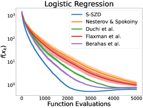
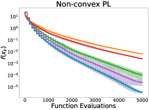
Figure 4: Comparison of finite differences algorithms in terms of function evaluations in four different problems. Results are plotted as mean $\pm$ standard deviation of $10$ repetitions.

In Figure 4, we can observe that S-SZD outperforms the other finite-differences methods in all problems. This result can be explained by observing that a gradient approximation built with Gaussian finite differences as in [40, 17] can be arbitrarily bad even when the directions chosen are near the direction of the gradient (this is because Gaussian distribution has infinite support). Note also that structured directions provide a better local exploration of the space than non-structured ones, reducing the probability to generate bad directions (i.e. when all directions chosen are far from the direction of the gradient). This result is also confirmed in terms of gradient accuracy in [4] where the authors empirically show that to obtain a gradient accuracy comparable to methods that use orthogonal directions, smoothing methods (Gaussian or spherical) can require significantly more samples.

C.4 Strategies to build direction matrices

We show here two examples of how to generate direction matrices $P_{k}$ for Algorithm 1. Specifically, we can have coordinate directions or spherical directions.
Coordinate Directions. The easiest way to build a direction matrix which satisfies Assumption 1 consists in taking the identity matrix $I\in\mathbb{R}^{d\times d}$ and sample $l$ columns uniformly at random (without replacement). Then for each sampled column, we flip the sign (we multiply by $-1$) with probability $1/2$ and we multiply the matrix by $\sqrt{d/l}$.
Spherical Directions. A different way to build a direction matrix satisfying Assumption 1, consists in taking directions orthogonal and uniform on a sphere [38]. The algorithm consists in generating a matrix $Z\in\mathbb{R}^{d\times d}$ s.t. $Z_{i,j}\sim\mathcal{N}(0,1)$ and computing the QR-decomposition. Then, the matrix $Q$ is truncated by taking the first $0<l\leq d$ directions and multiplied by $\sqrt{d/l}$.

Appendix D Limitations

In this appendix, we discuss the main limitations of Algorithm 1. A limitation of S-SZD consists in requiring multiple function evaluations to perform steps. Indeed, in many contexts, evaluating the function can be very time-expensive (e.g., running simulations). In such contexts, to get good performances in time, we would need to reduce $l$. However, as we observe in Section 4, we get worse performances. Moreover, in many practical scenarios, the stochastic objective function cannot be evaluated at different $x$ with the same $z$ (e.g., bandit feedback [20]). Also note that if the sequence $h_{k}$ decreases too fast we can have numerical instability in computing (2).

Appendix E Expanded discussion

In this appendix, we compare S-SZD 1 with stochastic zeroth order methods proposed in previous works. We compare convergence rates obtained for solving problem (1) considering different settings. In [40], the authors obtain a convergence rate of $\mathcal{O}({d}/{k}^{1/2})$ while with S-SZD, we obtain $\mathcal{O}(({d}/{l}){1/k^{1-c}})$ with $1/2<c<1$. Note that, with $l=1$ our algorithm almost recover that rate. Specifically, taking $c=1/2+\delta$ with $\delta>0$ small and $l=1$, our rate is arbitrary near to the rate in [40]. For $l>1$, we get a better dependence on dimension showing that taking more than one direction provides better performances. In [17], the authors propose a stochastic zeroth-order algorithm which approximates the gradient with a set of unstructured directions. The convergence rate in convex case is $\mathcal{O}\Big{(}(1+d/l)^{1/2}/k^{1/2}\Big{)}$. However, they obtain this rate by choosing the following parameters

$$\alpha_{k}=\frac{\alpha R}{2G\max\{\sqrt{d/l},1\}\sqrt{k}}\qquad\text{and}\qquad h_{k}=\frac{hG}{\lambda d^{3/2}k}$$

Note that the Lipschitz constant of the gradient $\lambda$ is included in the choice of parameters and this implies (in practice) that we should know it in order to use these parameters and thus obtain such rate. Moreover, their dependence on dimension appears to be better than our since they included a $({l/d})^{1/2}$ in the step-size. By including a $({l/d})^{1/2}$ in our step-size, we would improve our rate obtaining $\mathcal{O}((d/l)^{1/2}k^{c-1})$ - see discussion of Corollary 1. Note that the dependence on the iteration $k$ is slightly better than ours (depending on the choice of $c$). However, they considered a stricter setting than ours. Specifically, they assume that for every $x$, $\left\lVert{x-x^{*}}\right\rVert^{2}\leq(1/2)R^{2}$ for some $R<+\infty$ - see [17, Assumption A] while in our setting we do not make this assumption. Moreover, they assume that $\operatorname{\mathbb{E}}[\left\lVert{\nabla F(x,z)}\right\rVert^{2}]$ is uniformly bounded by a constant (see [17, Assumption B]) while our Assumption 3 (second equation) is more general. In Table 4 we summarize the convergence rates of S-SZD and [40, 17] including also the choice of parameters considered. We underline the fact that for [40] and [17] the non-convex case is not analyzed. Note that for the deterministic setting, the result obtained in [33] hold since our algorithm is its direct generalization to the stochastic setting.

Table 4: Comparison with finite-difference based algorithms in stochastic convex setting.

Algorithm	Rate	$\alpha_{k}$	$h_{k}$
Nesterov et al. [40]	$\mathcal{O}(\frac{d}{\sqrt{k}})$	see [40]	see [40]
Duchi et al. [17]	$\mathcal{O}(\sqrt{\frac{d}{l}}\frac{1}{\sqrt{k}})$	$\frac{\alpha R}{2G\max\{\sqrt{d/l},1\}\sqrt{k}}$	$\frac{hG}{\lambda d^{3/2}k}$
S-SZD	$\mathcal{O}(\frac{d}{l}\frac{1}{k^{1-c}})$	$\frac{\alpha}{k^{c}}$	$\frac{h}{k^{r}}$

References

• [1] Edward J. Anderson and Michael C. Ferris. A direct search algorithm for optimization with noisy function evaluations. SIAM Journal on Optimization, 11(3):837–857, 2001.
• [2] Jean Bernard Baillon and Georges Haddad. Quelques propriétés des opérateurs angle-bornés etn-cycliquement monotones. Israel Journal of Mathematics, 26(2):137–150, Jun 1977.
• [3] Krishnakumar Balasubramanian and Saeed Ghadimi. Zeroth-order (non)-convex stochastic optimization via conditional gradient and gradient updates. Advances in Neural Information Processing Systems, 31, 2018.
• [4] Albert S Berahas, Liyuan Cao, Krzysztof Choromanski, and Katya Scheinberg. A theoretical and empirical comparison of gradient approximations in derivative-free optimization. Foundations of Computational Mathematics, 22(2):507–560, 2022.
• [5] El Houcine Bergou, Eduard Gorbunov, and Peter Richtárik. Stochastic three points method for unconstrained smooth minimization. SIAM Journal on Optimization, 30(4):2726–2749, 2020.
• [6] Jérôme Bolte, Aris Daniilidis, Olivier Ley, and Laurent Mazet. Characterizations of Łojasiewicz inequalities: Subgradient flows, talweg, convexity. Transactions of The American Mathematical Society - TRANS AMER MATH SOC, 362:3319–3363, 06 2009.
• [7] Hanqin Cai, Yuchen Lou, Daniel Mckenzie, and Wotao Yin. A zeroth-order block coordinate descent algorithm for huge-scale black-box optimization. In Proceedings of the 38th International Conference on Machine Learning, volume 139 of Proceedings of Machine Learning Research, pages 1193–1203. PMLR, 18–24 Jul 2021.
• [8] HanQin Cai, Daniel McKenzie, Wotao Yin, and Zhenliang Zhang. Zeroth-order regularized optimization (zoro): Approximately sparse gradients and adaptive sampling. SIAM Journal on Optimization, 32(2):687–714, 2022.
• [9] Ruobing Chen and Stefan Wild. Randomized Derivative-Free Optimization of Noisy Convex Functions. arXiv e-prints, page arXiv:1507.03332, July 2015.
• [10] Krzysztof Choromanski, Mark Rowland, Vikas Sindhwani, Richard Turner, and Adrian Weller. Structured evolution with compact architectures for scalable policy optimization. In Jennifer Dy and Andreas Krause, editors, Proceedings of the 35th International Conference on Machine Learning, volume 80 of Proceedings of Machine Learning Research, pages 970–978. PMLR, 10–15 Jul 2018.
• [11] K. L. Chung. On a stochastic approximation method. The Annals of Mathematical Statistics, 25(3):463–483, 1954.
• [12] Andrew R. Conn, Katya Scheinberg, and Luís Nunes Vicente. Introduction to derivative-free optimization. In MPS-SIAM series on optimization, 2009.
• [13] M. Dodangeh and L. N. Vicente. Worst case complexity of direct search under convexity. Mathematical Programming, 155(1):307–332, Jan 2016.
• [14] M. Dodangeh, L. N. Vicente, and Zaikun Zhang. On the optimal order of worst case complexity of direct search. Optimization Letters, 10(4):699–708, April 2016.
• [15] Dheeru Dua and Casey Graff. UCI machine learning repository, 2017.
• [16] John C. Duchi, Peter L. Bartlett, and Martin J. Wainwright. Randomized smoothing for stochastic optimization. SIAM Journal on Optimization, 22(2):674–701, 2012.
• [17] John C. Duchi, Michael I. Jordan, Martin J. Wainwright, and Andre Wibisono. Optimal rates for zero-order convex optimization: The power of two function evaluations. IEEE Transactions on Information Theory, 61(5):2788–2806, 2015.
• [18] Abraham Flaxman, Adam Tauman Kalai, and Brendan McMahan. Online convex optimization in the bandit setting: Gradient descent without a gradient. In SODA ’05 Proceedings of the sixteenth annual ACM-SIAM symposium on Discrete algorithms, pages 385–394, January 2005.
• [19] Massimo Fornasier, Timo Klock, and Konstantin Riedl. Consensus-based optimization methods converge globally in mean-field law, 2021.
• [20] Peter I Frazier. A tutorial on bayesian optimization. arXiv preprint arXiv:1807.02811, 2018.
• [21] R. Garmanjani and L. N. Vicente. Smoothing and worst-case complexity for direct-search methods in nonsmooth optimization. IMA Journal of Numerical Analysis, 33(3):1008–1028, 2013.
• [22] Alexander Gasnikov, Anton Novitskii, Vasilii Novitskii, Farshed Abdukhakimov, Dmitry Kamzolov, Aleksandr Beznosikov, Martin Takac, Pavel Dvurechensky, and Bin Gu. The power of first-order smooth optimization for black-box non-smooth problems. In Proceedings of the 39th International Conference on Machine Learning, volume 162 of Proceedings of Machine Learning Research, pages 7241–7265. PMLR, 17–23 Jul 2022.
• [23] Geovani Nunes Grapiglia. Worst-case evaluation complexity of a derivative-free quadratic regularization method. 2022.
• [24] S. Gratton, C. W. Royer, L. N. Vicente, and Z. Zhang. Direct search based on probabilistic descent. SIAM Journal on Optimization, 25(3):1515–1541, 2015.
• [25] Jordan R. Hall and Varis Carey. Accelerating Derivative-Free Optimization with Dimension Reduction and Hyperparameter Learning. arXiv e-prints, page arXiv:2101.07444, January 2021.
• [26] Nikolaus Hansen. The CMA Evolution Strategy: A Comparing Review, volume 192, pages 75–102. 06 2007.
• [27] Charles R. Harris, K. Jarrod Millman, Stéfan J. van der Walt, Ralf Gommers, Pauli Virtanen, David Cournapeau, Eric Wieser, Julian Taylor, Sebastian Berg, Nathaniel J. Smith, Robert Kern, Matti Picus, Stephan Hoyer, Marten H. van Kerkwijk, Matthew Brett, Allan Haldane, Jaime Fernández del Río, Mark Wiebe, Pearu Peterson, Pierre Gérard-Marchant, Kevin Sheppard, Tyler Reddy, Warren Weckesser, Hameer Abbasi, Christoph Gohlke, and Travis E. Oliphant. Array programming with NumPy. Nature, 585(7825):357–362, September 2020.
• [28] J. Wolfowitz J. Kiefer. Stochastic estimation of the maximum of a regression function. The Annals of Mathematical Statistics, 23(3):462––466, 1952.
• [29] Sujin Kim and Dali Zhang. Convergence properties of direct search methods for stochastic optimization. pages 1003–1011, 12 2010.
• [30] Tamara G. Kolda, Robert Michael Lewis, and Virginia Torczon. Optimization by direct search: New perspectives on some classical and modern methods. SIAM Review, 45(3):385–482, 2003.
• [31] Jakub Konečný and Peter Richtárik. Simple complexity analysis of simplified direct search. Workingpaper, ArXiv, October 2014. 21 pages, 5 algorithms, 1 table.
• [32] David Kozák, Stephen Becker, Alireza Doostan, and Luis Tenorio. A stochastic subspace approach to gradient-free optimization in high dimensions. Comput. Optim. Appl., 79:339–368, 2021.
• [33] David Kozak, Cesare Molinari, Lorenzo Rosasco, Luis Tenorio, and Silvia Villa. Zeroth order optimization with orthogonal random directions, 2021.
• [34] R. J. Lyon, B. W. Stappers, S. Cooper, J. M. Brooke, and J. D. Knowles. Fifty years of pulsar candidate selection: from simple filters to a new principled real-time classification approach. Monthly Notices of the Royal Astronomical Society, 459(1):1104–1123, 04 2016.
• [35] Horia Mania, Aurelia Guy, and Benjamin Recht. Simple random search of static linear policies is competitive for reinforcement learning. In Proceedings of the 32nd International Conference on Neural Information Processing Systems, NIPS’18, page 1805–1814, Red Hook, NY, USA, 2018. Curran Associates Inc.
• [36] Giacomo Meanti, Luigi Carratino, Ernesto De Vito, and Lorenzo Rosasco. Efficient hyperparameter tuning for large scale kernel ridge regression. In Proceedings of The 25th International Conference on Artificial Intelligence and Statistics, 2022.
• [37] Giacomo Meanti, Luigi Carratino, Lorenzo Rosasco, and Alessandro Rudi. Kernel methods through the roof: Handling billions of points efficiently. In H. Larochelle, M. Ranzato, R. Hadsell, M. F. Balcan, and H. Lin, editors, Advances in Neural Information Processing Systems, volume 33, pages 14410–14422. Curran Associates, Inc., 2020.
• [38] Francesco Mezzadri. How to generate random matrices from the classical compact groups. Notices of the American Mathematical Society, 54:592–604, 10 2006.
• [39] Eric Moulines and Francis Bach. Non-asymptotic analysis of stochastic approximation algorithms for machine learning. In Advances in Neural Information Processing Systems, volume 24. Curran Associates, Inc., 2011.
• [40] Yurii Nesterov and Vladimir Spokoiny. Random gradient-free minimization of convex functions. Found. Comput. Math., 17(2):527–566, apr 2017.
• [41] Adam Paszke, Sam Gross, Francisco Massa, Adam Lerer, James Bradbury, Gregory Chanan, Trevor Killeen, Zeming Lin, Natalia Gimelshein, Luca Antiga, Alban Desmaison, Andreas Kopf, Edward Yang, Zachary DeVito, Martin Raison, Alykhan Tejani, Sasank Chilamkurthy, Benoit Steiner, Lu Fang, Junjie Bai, and Soumith Chintala. Pytorch: An imperative style, high-performance deep learning library. In Advances in Neural Information Processing Systems 32, pages 8024–8035. Curran Associates, Inc., 2019.
• [42] F. Pedregosa, G. Varoquaux, A. Gramfort, V. Michel, B. Thirion, O. Grisel, M. Blondel, P. Prettenhofer, R. Weiss, V. Dubourg, J. Vanderplas, A. Passos, D. Cournapeau, M. Brucher, M. Perrot, and E. Duchesnay. Scikit-learn: Machine learning in Python. Journal of Machine Learning Research, 12:2825–2830, 2011.
• [43] Boris T Polyak. Introduction to optimization. Optimization Software Inc., Publications Division, New York, 1:32, 1987.
• [44] Dobrivoje Popovic and Andrew R Teel. Direct search methods for nonsmooth optimization. In 2004 43rd IEEE Conference on Decision and Control (CDC)(IEEE Cat. No. 04CH37601), volume 3, pages 3173–3178. IEEE, 2004.
• [45] Christopher John Price, M Reale, and BL Robertson. A direct search method for smooth and nonsmooth unconstrained optimization. ANZIAM Journal, 48:C927–C948, 2006.
• [46] Marco Rando, Luigi Carratino, Silvia Villa, and Lorenzo Rosasco. Ada-bkb: Scalable gaussian process optimization on continuous domains by adaptive discretization. In Proceedings of The 25th International Conference on Artificial Intelligence and Statistics, volume 151 of Proceedings of Machine Learning Research, pages 7320–7348. PMLR, 28–30 Mar 2022.
• [47] H. Robbins and D. Siegmund. A convergence theorem for non negative almost supermartingales and some applications. In Jagdish S. Rustagi, editor, Optimizing Methods in Statistics, pages 233–257. Academic Press, 1971.
• [48] Lindon Roberts and Clément W. Royer. Direct search based on probabilistic descent in reduced spaces, 2022.
• [49] Lorenzo Rosasco, Silvia Villa, and Bang Công Vũ. Convergence of stochastic proximal gradient algorithm. Applied Mathematics & Optimization, 82(3):891–917, Dec 2020.
• [50] Alessandro Rudi, Luigi Carratino, and Lorenzo Rosasco. Falkon: An optimal large scale kernel method. In Advances in Neural Information Processing Systems, volume 30, 2017.
• [51] Sudeep Salgia, Sattar Vakili, and Qing Zhao. A domain-shrinking based bayesian optimization algorithm with order-optimal regret performance. In NeurIPS, 2021.
• [52] Tim Salimans, Jonathan Ho, Xi Chen, and Ilya Sutskever. Evolution strategies as a scalable alternative to reinforcement learning. ArXiv, abs/1703.03864, 2017.
• [53] Shubhanshu Shekhar and Tara Javidi. Gaussian process bandits with adaptive discretization. Electronic Journal of Statistics, 12(2):3829 – 3874, 2018.
• [54] Dr. Narinder Singh. Review of particle swarm optimization. International Journal of Computational Intelligence and Information Security, April 2012, Vol. 3:34–44, 01 2012.
• [55] James C. Spall. Introduction to Stochastic Search and Optimization. John Wiley & Sons, Inc., USA, 1 edition, 2003.
• [56] Niranjan Srinivas, Andreas Krause, Sham M Kakade, and Matthias Seeger. Gaussian process optimization in the bandit setting: No regret and experimental design. In Proceedings of the 27th International Conference on International Conference on Machine Learning, pages 1015–1022, 2010.
• [57] Claudia Totzeck. Trends in consensus-based optimization. In Active Particles, Volume 3, pages 201–226. Springer, 2022.