The Exactness of the $\ell_{1}$ Penalty Function for a Class of Mathematical Programs with Generalized Complementarity Constraints

Abstract

In a Mathematical Program with Generalized Complementarity Constraints (MPGCC), complementarity relationships are imposed between each pair of variable blocks. MPGCC includes the traditional Mathematical Program with Complementarity Constraints (MPCC) as a special case. On account of the disjunctive feasible region, MPCC and MPGCC are generally difficult to handle. The $\ell_{1}$ penalty method, often adopted in computation, opens a way of circumventing the difficulty. Yet it remains unclear about the exactness of the $\ell_{1}$ penalty function, namely, whether there exists a sufficiently large penalty parameter so that the penalty problem shares the optimal solution set with the original one. In this paper, we consider a class of MPGCCs that are of multi-affine objective functions. This problem class finds applications in various fields, e.g., the multi-marginal optimal transport problems in many-body quantum physics and the pricing problem in network transportation. We first provide an instance from this class, the exactness of whose $\ell_{1}$ penalty function cannot be derived by existing tools. We then establish the exactness results under rather mild conditions. Our results cover those existing ones for MPCC and apply to multi-block contexts.

1 Introduction

A Mathematical Program with Complementarity Constraints (MPCC) takes the form

$$\begin{array}[]{cl}\min\limits_{\mathbf{x},\mathbf{y}}&g(\mathbf{x},\mathbf{y})\\ \mathrm{s.}~{}\mathrm{t.}&\mathbf{h}(\mathbf{x},\mathbf{y})\leq 0,\\ &\mathbf{x}\geq 0,~{}\mathbf{y}\geq 0,~{}\left\langle\mathbf{x},\mathbf{y}\right\rangle=0,\end{array}$$ (1.1)

where $\mathbf{x}$, $\mathbf{y}\in\mathbb{R}^{m}$, $g:\mathbb{R}^{2m}\to\mathbb{R}$, and $\mathbf{h}:\mathbb{R}^{2m}\to\mathbb{R}^{q}$. MPCC has found wide applications in economics and engineering design. For a review on this topic, interested readers may refer to [27, 30] and the references therein. If $g$ and $\mathbf{h}$ are affine, the MPCC equation 1.1 reduces to a Linear Program with Complementarity Constraints (LPCC). For problems with multiple variable blocks, the complementarity relationships imposed between each block pair leads to the following Mathematical Program with Generalized Complementarity Constraints (MPGCC)

$$\begin{array}[]{cl}\min\limits_{\mathbf{x}_{1},\ldots,\mathbf{x}_{n}}&\tilde{g}(\mathbf{x}_{1},\ldots,\mathbf{x}_{n})\\ \mathrm{s.}~{}\mathrm{t.}&\tilde{\mathbf{h}}(\mathbf{x}_{1},\ldots,\mathbf{x}_{n})\leq 0,\\ &\mathbf{x}_{i}\geq 0,~{}i=1,\ldots,n,\\ &\left\langle\mathbf{x}_{i},\mathbf{x}_{j}\right\rangle=0,~{}\forall~{}i,j\in\{1,\ldots,n\}:i\neq j,\end{array}$$ (1.2)

where $\mathbf{x}_{i}\in\mathbb{R}^{m}$ for $i=1,\ldots,n$, $\tilde{g}:\mathbb{R}^{mn}\to\mathbb{R}$, and $\tilde{\mathbf{h}}:\mathbb{R}^{mn}\to\mathbb{R}^{q}$.

It is worth mentioning that MPCC equation 1.1 and MPGCC equation 1.2 violate standard constraint qualifications at any feasible point, such as the Mangasarian-Fromovitz constraint qualification (MFCQ) [16]. Consequently, the local solutions, and of course optimal solutions, do not necessarily satisfy the associated Karush-Kuhn-Tucker conditions, which renders these problems particularly difficult to cope with. It can also be proved that globally solving a general MPCC or MPGCC is NP-complete [11, 20, 23]. To this end, several tailored constraint qualifications and stationarity notions have been proposed for MPCC; see [15, 16, 17, 19, 29, 32, 34] for example.

Instead of facing the original MPCC equation 1.1 or MPGCC equation 1.2, one could alternatively penalize the (generalized) complementarity constraints using $\ell_{1}$ penalty term, and then turn to consider the penalty problem. Taking the MPGCC equation 1.2 as an instance, we write its $\ell_{1}$ penalty counterpart as

$$\begin{array}[]{cl}\min\limits_{\mathbf{x}_{1},\ldots,\mathbf{x}_{n}}&\tilde{g}_{\beta}(\mathbf{x}_{1},\ldots,\mathbf{x}_{n}):=\tilde{g}(\mathbf{x}_{1},\ldots,\mathbf{x}_{n})+\beta p(\mathbf{x}_{1},\ldots,\mathbf{x}_{n})\\ \mathrm{s.}~{}\mathrm{t.}&\tilde{\mathbf{h}}(\mathbf{x}_{1},\ldots,\mathbf{x}_{n})\leq 0;~{}\mathbf{x}_{i}\geq 0,~{}i=1,\ldots,n,\end{array}$$ (1.3)

where $\beta>0$ refers to the penalty parameter and the $\ell_{1}$ penalty term

$$p(\mathbf{x}_{1},\ldots,\mathbf{x}_{n}):=\sum_{i=1}^{n}\sum_{j>i}\left\langle\mathbf{x}_{i},\mathbf{x}_{j}\right\rangle,\quad\forall~{}\mathbf{x}_{1},\ldots,\mathbf{x}_{n}\in\mathbb{R}^{m}.$$ (1.4)

The penalty problem equation 1.3 enjoys several nice properties: (i) there is no need to take absolute value for $p$ because of the nonnegative constraints and, therefore, no nonsmoothness is introduced; (ii) the problem equation 1.3 is free of complementarity constraints and standard constraint qualifications may readily hold. Nevertheless, it remains unclear about the exactness of the $\ell_{1}$ penalty function, i.e., whether or not the optimal solution sets of equation 1.2 and equation 1.3 coincide for all sufficiently large $\beta$.

In this paper, we consider a class of MPGCC that reads

$$\begin{array}[]{cl}\displaystyle\min_{\mathbf{x}_{1},\ldots,\mathbf{x}_{n}}&\displaystyle f(\mathbf{x}_{1},\ldots,\mathbf{x}_{n})\\ \mathrm{s.}~{}\mathrm{t.}&\mathbf{x}_{i}\in\Omega_{i},~{}\mathbf{x}_{i}\geq 0,~{}i=1,\ldots,n,\\ &\left\langle\mathbf{x}_{i},\mathbf{x}_{j}\right\rangle=0,~{}\forall~{}i,j\in\{1,\ldots,n\}:i\neq j.\end{array}\Hy@raisedlink{\hypertarget{MPGCC}{}}$$ (P)

Here $f:\mathbb{R}^{mn}\to\mathbb{R}$ is multi-affine, i.e., for $i=1,\ldots,n$, it is affine with respect to $\mathbf{x}_{i}$ after fixing the other $n-1$ blocks. The sets $\{\Omega_{i}\}_{i=1}^{n}$ are polyhedrons in $\mathbb{R}^{m}$. In the sequel, we denote the feasible region of equation P by $\mathcal{F}$ and let $\mathbf{z}:=(\mathbf{x}_{1},\ldots,\mathbf{x}_{n})\in\mathbb{R}^{mn}$, $\Omega_{i}^{+}:=\Omega_{i}\cap\mathbb{R}^{m}_{+}$ ($i=1,\ldots,n$) for brevity.

The relationships among the general LPCC, MPCC, MPGCC as well as the scope of the model equation P are depicted in Figure 1. The cyan ellipsoid with solid boundary stands for MPGCC, the larger cyan disk with dashed boundary for MPCC, and the smaller cyan disk with dotted boundary for LPCC. The red ellipsoid with dashdotted boundary refers to the scope of the model equation P.

Figure 1: Relationships among the general LPCC, MPCC, MPGCC as well as the scope of equation P.

The model equation P can be found in various fields. In [21, 22], the authors formulate the discretized multi-marginal optimal transport problems arising in quantum physics under the so-called Monge-like ansatz into an MPGCC as equation P. The generalized complementarity constraints are present to prevent the unfavorable clustering of electrons. As an LPCC or MPCC, equation P is able to model sequential decision processes such as pricing in network taxation [7, 8, 24, 25], biofuel production [2], airline industry [13], and telecommunication services [4, 5, 6].

Similar to equation 1.3, the $\ell_{1}$ penalized equation P reads

$$\min_{\mathbf{z}}~{}f_{\beta}(\mathbf{z}):=f(\mathbf{z})+\beta p(\mathbf{z}),\quad\mathrm{s.}~{}\mathrm{t.}~{}\mathbf{x}_{i}\in\Omega_{i}^{+},~{}i=1,\ldots,n.$$ (P_β)

Recall that $p$ is defined in equation 1.4. We denote the feasible region of equation P_β as $\Omega:=\prod_{i=1}^{n}\Omega_{i}^{+}$, where “$\prod$” stands for the Cartesian product among sets.

The aim of this paper is to establish the exactness of the $\ell_{1}$ penalty function for equation P via exploring the relationship between the optimal solution sets of equation P and equation P_β. The global optimization algorithms for equation P and equation P_β go beyond the range of this work.

1.1 Literature Review

We review in this part the literatures on the exactness of the $\ell_{1}$ penalty function for MPGCC. These existing results can be divided into two parts: one is devoted to the general MPCC equation 1.1, while the other focuses on the special cases of the model equation P. The limitations are gathered at the end of each part, from which we draw our motivation.

For the general MPCC equation 1.1, one could establish the exactness of the $\ell_{1}$ penalty function by imposing additional regularity assumptions. In [27, 28], the authors analyze the exactness with the aid of the strict complementarity condition and the following error bound

$$\exists~{}\tau>0,~{}\mathrm{s.}~{}\mathrm{t.}~{}\mathrm{dist}\left((\mathbf{x},\mathbf{y}),\tilde{\mathcal{F}}\right)\leq\tau\left\langle\mathbf{x},\mathbf{y}\right\rangle,\quad\forall~{}(\mathbf{x},\mathbf{y})\in\tilde{\Omega},$$ (1.5)

where $\tilde{\mathcal{F}}$ and $\tilde{\Omega}$ refer to the feasible regions of equation 1.2 and equation 1.3, respectively. Here the strict complementarity condition means that $\mathbf{x}+\mathbf{y}>0$ for any $(\mathbf{x},\mathbf{y})\in\tilde{\mathcal{F}}$. Later on, the authors of [26] establish the exactness under the so-called positive-multiplier nondegeneracy condition and the MFCQ of the penalty problem. The above mentioned regularity assumptions may appear to be restrictive. The strict complementarity condition in [27, 28] can easily fail for a general MPCC [21, 26]. Moreover, it is nontrivial to check priorly whether the nondegeneracy condition in [26] holds at the points of interest. As for the general MPGCC equation 1.2, the theoretical properties of the $\ell_{1}$ penalty function have not yet been investigated.

There are also works dedicated to the $\ell_{1}$ exact penalty for equation P with affine objectives and two variable blocks. The authors of [9, 10] show the exactness based upon the finiteness of extreme point sets; see also earlier works [1, 24, 25, 33], where any optimal solution of equation P is proved to solve equation P_β but the reverse direction is ignored. All the works just mentioned concentrate on equation P with affine objectives and two variable blocks, while no theoretical results are known for the $n>2$ cases or when the objectives are nonlinear. Nevertheless, the authors of [21] report rather encouraging numerical results in solving an MPGCC as equation P via the $\ell_{1}$ penalty method.

To sum up, the limitations of the existing works motivate us to pursue the $\ell_{1}$ penalty exactness result on equation P with arbitrary $n\geq 2$ and nonlinear objectives under weaker assumptions than those in [26, 27, 28].

1.2 Contributions

We provide an example of equation P, the exactness of whose $\ell_{1}$ penalty function cannot be implied by the existing results. Leveraging on the special structure of equation P, we show the exactness of the $\ell_{1}$ penalty function under a rather mild assumption. Our results cover those for LPCC in [1, 9, 10, 24, 25, 33] and applies to the multi-block settings with nonlinear objectives. For a view of our position, please refer to the red ellipsoid in Figure 1.

1.3 Notations and Organization

We denote scalars, vectors, and matrices by lower-case letters, bold lower-case letters, and upper-case letters, respectively. The notations $\mathbf{1}$ and $I$ stand for the all-one vector and identity matrix in proper dimension, respectively. The support of a matrix $X=(X_{ij})$ is presented by $\mathrm{supp}(X):=\{(i,j):X_{ij}\neq 0\}$. We use “$\mathrm{vec}(\cdot)$” to vectorize matrices by column stacking. The Kronecker product between two matrices is denoted by “$\otimes$”. The operator “$\left\langle\cdot,\cdot\right\rangle$” represents the standard inner product of two vectors or matrices, while “$\|\cdot\|$” represents the induced norm.

We denote respectively the extreme point sets of $\Omega_{i}^{+}$ by $\overline{\Omega_{i}^{+}}$ for $i=1,\ldots,n$, the extreme point set of $\Omega$ by $\bar{\Omega}$, the optimal solution set of equation P by $S^{\mathrm{opt}}$, and the optimal solution set of equation P_β by $S_{\beta}^{\mathrm{opt}}$ for any $\beta\in\mathbb{R}$. Let $\bar{S}^{\mathrm{opt}}:=\bar{\Omega}\cap S^{\mathrm{opt}}$ and $\bar{S}_{\beta}^{\mathrm{opt}}:=\bar{\Omega}\cap S_{\beta}^{\mathrm{opt}}$ denote the extreme-point optimal solution of equation P and equation P_β, respectively. The cardinality of a set $S$ is represented by $\left|S\right|$. The line segment connected by two points, $\mathbf{a}$ and $\mathbf{b}$, is denoted by $\ell(\mathbf{a},\mathbf{b}):=\{(1-\lambda)\mathbf{a}+\lambda\mathbf{b}:\lambda\in[0,1]\}$. The notation $\mathrm{rbd}~{}S$ refers to the relative boundary of a set $S$. The distance between a point $\mathbf{a}$ and a closed set $S$ is represented by $\mathrm{dist}(\mathbf{a},S):=\min_{\mathbf{w}\in S}\|\mathbf{a}-\mathbf{w}\|$.

We organize this paper as follows. The example of equation P falling outside the literatures is detailed in section 2. The main results of the $\ell_{1}$ penalty exactness on equation P are elaborated in section 3. We draw conclusions and perspectives in section 4.

2 The $\ell_{1}$ Penalty Exactness beyond the Existing Works

We give an instance of equation P, related to real applications [21, 22], whose $\ell_{1}$ penalty exactness cannot be implied by the existing works. Specifically, it is not an LPCC analyzed in [1, 9, 10, 24, 25, 33]. Moreover, neither the strict complementarity condition nor the error bound equation 1.5 in [27, 28] is satisfied.

Consider the following MPCC with three matrix variables

$$\begin{array}[]{cl}\min\limits_{Z}&\displaystyle\sum_{i=1}^{3}\left\langle X_{i},C\right\rangle+\sum_{i=1}^{3}\sum_{j>i}\left\langle X_{i},X_{j}C\right\rangle\\ \mathrm{s.}~{}\mathrm{t.}&X_{i}\mathbf{1}=\mathbf{1},~{}X_{i}^{\top}\mathbf{1}=\mathbf{1},~{}\mathrm{Tr}(X_{i})=0,~{}X_{i}\geq 0,~{}i=1,2,3,\\ &\left\langle X_{1},X_{2}\right\rangle=0,~{}\left\langle X_{1},X_{3}\right\rangle=0,~{}\left\langle X_{2},X_{3}\right\rangle=0,\end{array}$$ (2.1)

where $K\in\mathbb{N}$, $X_{1}$, $X_{2}$, $X_{3}\in\mathbb{R}^{K\times K}$, $Z:=(X_{1},X_{2},X_{3})\in\prod_{i=1}^{3}\mathbb{R}^{K\times K}$, $C=(C_{ij})\in\mathbb{R}^{K\times K}$ is defined as

$$C_{ij}=\left\{\begin{array}[]{ll}\dfrac{1}{\left|i-j\right|h},&\text{if}~{}i\neq j,\\ 0,&\text{otherwise}\end{array}\right.~{}\text{with}~{}h:=\frac{1}{K}.$$

The problem equation 2.1 is in the form of equation P with $n=3$, $m=K^{2}$, $\mathbf{x}_{i}=\mathrm{vec}(X_{i})$ ($i=1,2,3$), $f(\mathbf{z})=\sum_{i=1}^{3}\left\langle\mathbf{a},\mathbf{x}_{i}\right\rangle+\sum_{i=1}^{3}\sum_{j>i}\left\langle\mathbf{x}_{i},R\mathbf{x}_{j}\right\rangle$, $\mathbf{a}=\mathrm{vec}(C)$, $R=\frac{1}{2}\begin{bmatrix}0&C\otimes I\\ C\otimes I&0\end{bmatrix}$, and

$$\Omega_{1}=\Omega_{2}=\Omega_{3}=\left\{\mathbf{w}\in\mathbb{R}^{K^{2}}:\begin{bmatrix}\mathbf{1}^{\top}\otimes I\\ I\otimes\mathbf{1}^{\top}\\ \mathrm{vec}(I)^{\top}\end{bmatrix}\mathbf{w}=\begin{bmatrix}\mathbf{1}\\ \mathbf{1}\\ 0\end{bmatrix}\right\},~{}\mathcal{F}=\left\{\mathbf{z}\in\prod_{i=1}^{3}\Omega_{i}^{+}:p(\mathbf{z})=0\right\}.$$

This instance is derived from the one-dimensional multi-marginal optimal transport model arising in many-body quantum physics [21, 22], particularly with four electrons, constant density, and uniform discretization over the interval $[0,1]$. By [12], if $K$ can be divided by $4$, we are able to explicitly write down one optimal solution $Z^{*}:=(X_{1}^{*},X_{2}^{*},X_{3}^{*})$ to equation 2.1:

$$(X_{1}^{*})_{ij} =\left\{\begin{array}[]{ll}1,&\text{if}~{}i-j=\frac{3K}{4}~{}\text{or}~{}j-i=\frac{K}{4},\\ 0,&\text{otherwise},\end{array}\right.$$ (2.4)

$$(X_{2}^{*})_{ij} =\left\{\begin{array}[]{ll}1,&\text{if}~{}i-j=\frac{K}{2},~{}\text{or}~{}j-i=\frac{K}{2},\\ 0,&\text{otherwise},\end{array}\right.$$ (2.7)

$$(X_{3}^{*})_{ij} =\left\{\begin{array}[]{ll}1,&\text{if}~{}i-j=\frac{K}{4}~{}\text{or}~{}j-i=\frac{3K}{4},\\ 0,&\text{otherwise}.\end{array}\right.$$ (2.10)

An illustration of $Z^{*}$ can be found in Figure 2.

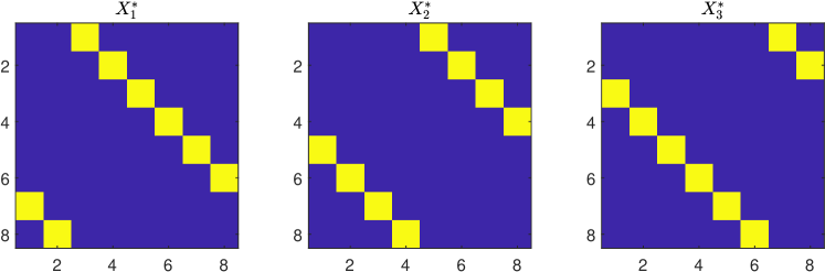
Figure 2: The illustration of $Z^{*}$ when $K=8$. Each yellow block stands for the value of $1$, while each deep blue block for the value of $0$.

Since $n>2$ and $f$ is nonlinear, equation 2.1 cannot be covered by the existing works on the special cases of equation P. Moreover, the strict complementarity condition is violated on equation 2.1 due to the zero-trace constraints. Next, we argue that the error bound equation 1.5 fails to hold on equation 2.1 whenever $K>4$ and $\bmod(K,4)=0$.

Theorem 1.

For equation 2.1 with $K:K>4$ and $\bmod(K,4)=0$, there does not exist $\tau>0$ such that

$$\mathrm{dist}(Z,\mathcal{F})\leq\tau p(Z),\quad\forall~{}Z\in\Omega.$$ (2.11)

Proof.

In light of the optimal solution $Z^{*}$ in equation 2.7, for any $\varepsilon\in(0,1)$, we come up with $Z(\varepsilon):=(X_{1}(\varepsilon),X_{2}^{*},X_{3}(\varepsilon))$ (see Figure 3 for illustration) where $X_{1}(\varepsilon)$ and $X_{3}(\varepsilon)$ are defined as

$$(X_{1}(\varepsilon))_{ij} =\left\{\begin{array}[]{ll}1-\varepsilon,&\text{if}~{}i-j=\frac{3K}{4}~{}\text{or}~{}j-i=\frac{K}{4},\\ \varepsilon,&\text{if}~{}i-j=\frac{3K}{4}-1~{}\text{or}~{}j-i=\frac{K}{4}+1,\\ 0,&\text{otherwise},\end{array}\right.$$

$$(X_{3}(\varepsilon))_{ij} =\left\{\begin{array}[]{ll}1-\varepsilon,&\text{if}~{}i-j=\frac{K}{4}~{}\text{or}~{}j-i=\frac{3K}{4},\\ \varepsilon,&\text{if}~{}i-j=\frac{3K}{4}-1~{}\text{or}~{}j-i=\frac{K}{4}+1,\\ 0,&\text{otherwise}.\end{array}\right.$$

It is easy to verify that $Z(\varepsilon)\in\Omega$ but $p(Z(\varepsilon))=K\varepsilon^{2}$ for any $\varepsilon\in(0,1)$ (since $K>4$), and $Z(\varepsilon)\to Z^{*}$ as $\varepsilon\to 0+$.

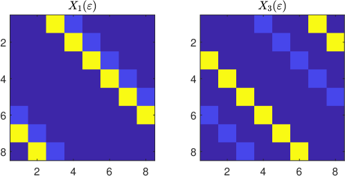
Figure 3: The illustration of $X_{1}(\varepsilon)$ and $X_{3}(\varepsilon)$ when $K=8$. Each yellow block stands for the value of $1-\varepsilon$, each light blue block for the value of $\varepsilon$, while each deep blue block for the value of $0$.

If it happens that $Z^{*}\in\operatorname*{arg\,min}_{Z\in\mathcal{F}}\|Z-Z(\varepsilon)\|$, then

$$\mathrm{dist}(Z(\varepsilon),\mathcal{F})=\|Z^{*}-Z(\varepsilon)\|=2\sqrt{K}\varepsilon=\frac{2}{\sqrt{K}\varepsilon}p(Z(\varepsilon)).$$

Passing $\varepsilon\to 0+$ yields the nonexistence of a uniform $\tau>0$ in equation 2.11.

If $Z^{*}\notin\operatorname*{arg\,min}_{Z\in\mathcal{F}}\|Z-Z(\varepsilon)\|$, we will show that

$$\limsup_{\varepsilon\to 0+}\frac{\mathrm{dist}(Z(\varepsilon),\mathcal{F})}{\varepsilon}>0,$$ (2.12)

leading again to the failure of equation 2.11. Suppose otherwise that

$$\mathrm{dist}(Z(\varepsilon),\mathcal{F})=\|\tilde{Z}(\varepsilon)-Z(\varepsilon)\|=o(\varepsilon)~{}\text{as}~{}\varepsilon\to 0+,$$ (2.13)

where $\tilde{Z}(\varepsilon):=(\tilde{X}_{1}(\varepsilon),\tilde{X}_{2}(\varepsilon),\tilde{X}_{3}(\varepsilon))\in\mathcal{F}$. Since the nonzero entries of $X_{1}(\varepsilon)$ and $X_{3}(\varepsilon)$ are either $1-\varepsilon$ or $\varepsilon$ and, by equation 2.13, $\left|(X_{i}(\varepsilon))_{jk}-(\tilde{X}_{i}(\varepsilon))_{jk}\right|=o(\varepsilon)$ for $i=1,3$ and $j,k=1,\ldots,K$, we know that $\mathrm{supp}(\tilde{X}_{i}(\varepsilon))\supseteq\mathrm{supp}(X_{i}(\varepsilon))$ for $i=1,3$. Note that $\tilde{X}_{1}(\varepsilon)$, $\tilde{X}_{3}(\varepsilon)\geq 0$. Hence, $\left\langle\tilde{X}_{1}(\varepsilon),\tilde{X}_{3}(\varepsilon)\right\rangle>0$ because $\left\langle X_{1}(\varepsilon),X_{3}(\varepsilon)\right\rangle>0$. This contradicts with $\tilde{Z}(\varepsilon)\in\mathcal{F}$ and validates equation 2.12. Combining the above two cases, we complete the proof. ∎

As a result, the exactness of the $\ell_{1}$ penalty function for equation P cannot be achieved as in the literatures [1, 9, 10, 24, 25, 27, 28, 33]. We next rigorously prove this exactness under a rather mild assumption by exploiting the structure of equation P.

3 Main Results

In this part, we elaborate the proof of $\ell_{1}$ penalty exactness on equation P. For a reference of notations, please look back to subsection 1.3. We make the following weak assumption on $\Omega$ hereafter.

Assumption 1.

The set $\Omega$ is nonempty and compact.

Assumption 1 usually automatically holds in real applications [21, 24]. With this assumption, the attainment of the optimal value of equation P_β for any $\beta\in\mathbb{R}$ is ensured.

The first result states that, for any $\beta\in\mathbb{R}$, $\bar{S}^{\mathrm{opt}}_{\beta}\neq\emptyset$, i.e., there exists at least one extreme-point optimal solution for equation P_β. Its proof hinges on the multi-affine structure of $f_{\beta}$ and the separability of $\Omega$ with respect to variable blocks.

Lemma 1.

Suppose Assumption 1 holds. Then $\bar{S}^{\mathrm{opt}}_{\beta}\neq\emptyset$ for any $\beta\in\mathbb{R}$.

Proof.

By Assumption 1, $S_{\beta}^{\mathrm{opt}}\neq\emptyset$ for any $\beta\in\mathbb{R}$. Pick $\hat{\mathbf{z}}:=(\hat{\mathbf{x}}_{1},\ldots,\hat{\mathbf{x}}_{n})\in S^{\mathrm{opt}}_{\beta}$. If it happens that $\hat{\mathbf{z}}\in\bar{\Omega}$, we are done. Otherwise, consider a linear program

$$\min_{\mathbf{x}_{1}\in\Omega_{1}^{+}}~{}~{}f_{\beta}(\mathbf{x}_{1},\hat{\mathbf{x}}_{2},\ldots,\hat{\mathbf{x}}_{n}).$$ (3.1)

Let $\mathbf{x}_{1}^{*}\in\overline{\Omega_{1}^{+}}$ be its extreme-point optimal solution, whose existence is guaranteed by Bauer maximum principle [3] and Assumption 1. Then by the optimality of $\mathbf{x}_{1}^{*}$ and the feasibility of $\hat{\mathbf{x}}_{1}$, one has $f_{\beta}(\mathbf{x}_{1}^{*},\hat{\mathbf{x}}_{2},\ldots,\hat{\mathbf{x}}_{n})\leq f_{\beta}(\hat{\mathbf{x}}_{1},\ldots,\hat{\mathbf{x}}_{n})$. Next, for any $j\geq 2$, consider successively linear program of the form

$$\min_{\mathbf{x}_{j}\in\Omega_{j}^{+}}~{}~{}f_{\beta}(\mathbf{x}_{1}^{*},\ldots,\mathbf{x}_{j-1}^{*},\mathbf{x}_{j},\hat{\mathbf{x}}_{j+1},\ldots,\hat{\mathbf{x}}_{n}),$$

and let $\mathbf{x}_{j}^{*}\in\overline{\Omega_{j}^{+}}$ be its extreme-point optimal solution, whose existence is ensured similarly. Clearly, it holds, for any $j\in\{2,\ldots,n\}$, that

$$f_{\beta}(\mathbf{x}_{1}^{*},\ldots,\mathbf{x}_{j-1}^{*},\mathbf{x}_{j}^{*},\hat{\mathbf{x}}_{j+1},\ldots,\hat{\mathbf{x}}_{n})\leq f_{\beta}(\mathbf{x}_{1}^{*},\ldots,\mathbf{x}_{j-1}^{*},\hat{\mathbf{x}}_{j},\hat{\mathbf{x}}_{j+1},\ldots,\hat{\mathbf{x}}_{n}).$$

Together, we have a chain

$$f_{\beta}(\mathbf{x}_{1}^{*},\ldots,\mathbf{x}_{n}^{*})\leq f_{\beta}(\mathbf{x}_{1}^{*},\ldots,\hat{\mathbf{x}}_{n})\leq\cdots\leq f_{\beta}(\mathbf{x}_{1}^{*},\hat{\mathbf{x}}_{2},\ldots,\hat{\mathbf{x}}_{n})\leq f_{\beta}(\hat{\mathbf{x}}_{1},\ldots,\hat{\mathbf{x}}_{n}).$$

Note that due to the separability of $\Omega$, $\bar{\Omega}=\prod_{i=1}^{n}\overline{\Omega_{i}^{+}}$ and $\mathbf{z}^{*}:=(\mathbf{x}_{1}^{*},\ldots,\mathbf{x}_{n}^{*})\in\bar{\Omega}$. Moreover, since $\hat{\mathbf{z}}$ is an optimal solution of equation P_β, one has $\mathbf{z}^{*}\in S^{\mathrm{opt}}_{\beta}$ in view of the last inequality chain. This completes the proof. ∎

Utilizing the finiteness of $\bar{\Omega}$ and Lemma 1, we could show the following partial exact penalty result.

Theorem 2.

Suppose Assumption 1 holds. Then there exists $\bar{\beta}>0$ such that $\bar{S}^{\mathrm{opt}}_{\beta}\subseteq S^{\mathrm{opt}}\subseteq S^{\mathrm{opt}}_{\beta}$ for any $\beta\geq\bar{\beta}$.

Proof.

We begin with the proof of $\bar{S}_{\beta}^{\mathrm{opt}}\subseteq S^{\mathrm{opt}}$ for all sufficiently large $\beta$ by contradiction. Suppose that there exists $\{\beta^{(k)}>0\}\to\infty$ and a corresponding $\{\mathbf{z}^{(k)}\}\subseteq\bar{S}_{\beta^{(k)}}^{\mathrm{opt}}\setminus S^{\mathrm{opt}}$ (due to Lemma 1). Clearly, if $\mathbf{z}\in S_{\beta}^{\mathrm{opt}}$ for some $\beta>0$ and $p(\mathbf{z})=0$, then $\mathbf{z}\in S^{\mathrm{opt}}$. It then holds that $p(\mathbf{z}^{(k)})>0$ for each $k$. Since $\{\Omega_{i}^{+}\}_{i=1}^{n}$ are polyhedral, one has $\left|\bar{\Omega}\right|<\infty$ and

$$\inf_{l}f(\mathbf{z}^{(l)})>-\infty~{}\text{and}~{}\inf_{l}p(\mathbf{z}^{(l)})>0.$$ (3.2)

Given any $\mathbf{z}$ feasible for equation P, it holds, for any $k$, that

$$\infty>f(\mathbf{z}) =f(\mathbf{z})+\beta^{(k)}p(\mathbf{z})\geq f_{\beta^{(k)}}(\mathbf{z}^{(k)})$$

$$=f(\mathbf{z}^{(k)})+\beta^{(k)}p(\mathbf{z}^{(k)})$$

$$\geq\inf_{l}f(\mathbf{z}^{(l)})+\beta^{(k)}\inf_{l}p(\mathbf{z}^{(l)}).$$

Based upon equation 3.2, we reach a contradiction after passing $k$ to $\infty$ in the last inequality. Therefore, there exists $\bar{\beta}>0$ such that $\bar{S}_{\beta}^{\mathrm{opt}}\subseteq S^{\mathrm{opt}}$ holds for any $\beta\geq\bar{\beta}$.

Now we show the second inclusion, i.e., given $\beta\geq\bar{\beta}$, for any $\mathbf{z}^{*}\in S^{\mathrm{opt}}$ and $\mathbf{z}\in\Omega$, $f_{\beta}(\mathbf{z}^{*})\leq f_{\beta}(\mathbf{z})$. By Lemma 1, $\bar{S}_{\beta}^{\mathrm{opt}}\neq\emptyset$. Pick $\hat{\mathbf{z}}\in\bar{S}_{\beta}^{\mathrm{opt}}$. From the first inclusion, we know that $\hat{\mathbf{z}}\in S^{\mathrm{opt}}$. Hence $f_{\beta}(\mathbf{z}^{*})=f(\mathbf{z}^{*})=f(\hat{\mathbf{z}})=f_{\beta}(\hat{\mathbf{z}})$. Since $\hat{\mathbf{z}}\in S^{\mathrm{opt}}_{\beta}$, we further have $f_{\beta}(\hat{\mathbf{z}})\leq f_{\beta}(\mathbf{z})$. Combining with the last equality chain, one concludes that $f_{\beta}(\mathbf{z}^{*})\leq f_{\beta}(\mathbf{z})$. ∎

To complete the exactness, it suffices to show the reverse direction: $S_{\beta}^{\mathrm{opt}}\subseteq S^{\mathrm{opt}}$. We begin with the following lemma, which states that the optimal solution of equation P_β with only one non-extreme variable block must be optimal for equation P.

Lemma 2.

Suppose Assumption 1 holds. For a given $\beta\geq\bar{\beta}$, let $\hat{\mathbf{z}}:=(\hat{\mathbf{x}}_{1},\ldots,\hat{\mathbf{x}}_{n})\in S_{\beta}^{\mathrm{opt}}$. If there exists only one index $i\in\{1,\ldots,n\}$ such that $\hat{\mathbf{x}}_{i}\notin\overline{\Omega_{i}^{+}}$, then $\hat{\mathbf{z}}\in S^{\mathrm{opt}}$.

Proof.

Without loss of generality, we assume $i=1$. Suppose, on the contrary, that $\hat{\mathbf{z}}\notin S^{\mathrm{opt}}$. Then we must have $p(\hat{\mathbf{z}})>0$. Since $\hat{\mathbf{z}}\in S_{\beta}^{\mathrm{opt}}$, $\hat{\mathbf{x}}_{1}$ solves the linear program equation 3.1 and $\hat{\mathbf{x}}_{1}\in\mathrm{rbd}~{}\Omega_{1}^{+}$. Due to $\hat{\mathbf{x}}_{1}\notin\overline{\Omega_{1}^{+}}$, equation 3.1 is degenerate on a face, say $\hat{F}_{1}$, of $\Omega_{1}^{+}$ where $\hat{\mathbf{x}}_{1}$ lies and, therefore, each point in $\hat{F}_{1}$ solves equation 3.1. In particular, by Theorem 2, each extreme point of $\hat{F}_{1}$, together with $\{\hat{\mathbf{x}}_{j}\}_{j=2}^{n}$, solves equation P. Denote by $\{\bar{\mathbf{x}}_{1}^{(i)}\}_{i\in\hat{I}_{1}}$ the extreme points of $\hat{F}_{1}$, where $\hat{I}_{1}\subseteq\mathbb{N}$ is a finite index set. Note that $\hat{F}_{1}$ is convex compact. By Minkowski’s theorem (see, e.g., [31, Corollary 18.5.1]), $\hat{F}_{1}$ is the convex hull of $\{\bar{\mathbf{x}}_{1}^{(i)}\}_{i\in\hat{I}_{1}}$. Since $\hat{\mathbf{x}}_{1}\notin\overline{\Omega_{1}^{+}}$, $\left|\hat{I}_{1}\right|\geq 2$.

Pick any two elements in $\hat{I}_{1}$, e.g., $i=1,2$. Then $(\bar{\mathbf{x}}_{1}^{(i)},\hat{\mathbf{x}}_{2},\ldots,\hat{\mathbf{x}}_{n})\in S^{\mathrm{opt}}$ and $p(\bar{\mathbf{x}}_{1}^{(i)},\hat{\mathbf{x}}_{2},\ldots,\hat{\mathbf{x}}_{n})=0$ for $i=1,2$. Since the function $p$ is linear with respect to the first block, one must have $p(\mathbf{x}_{1},\hat{\mathbf{x}}_{2},\ldots,\hat{\mathbf{x}}_{n})=0$ for any $\mathbf{x}_{1}\in\ell(\bar{\mathbf{x}}_{1}^{(1)},\bar{\mathbf{x}}_{1}^{(2)})$.

Invoking the arguments in the former paragraph repeatedly, we could deduce that the function $p\equiv 0$ on $\mathrm{rbd}~{}\hat{F}_{1}$. If $\hat{\mathbf{x}}_{1}\in\mathrm{rbd}~{}\hat{F}_{1}$, we then reach a contradiction. Otherwise, since $\hat{F}_{1}$ is convex compact, $\hat{\mathbf{x}}_{1}$ must lies on the line segment connected by two points in $\mathrm{rbd}~{}\hat{F}_{1}$. Again, since $p$ is linear with respect to the first block, $p(\hat{\mathbf{z}})=0$, leading to a contradiction. The proof is complete. ∎

We then prove the exactness result by mathematical induction.

Theorem 3.

Suppose Assumption 1 holds. For a given $\beta\geq\bar{\beta}$, $S_{\beta}^{\mathrm{opt}}=S^{\mathrm{opt}}$.

Proof.

The “$\supseteq$” part is ensured by Theorem 2. Below, we deal with the “$\subseteq$” part. We prove by mathematical induction that, for $r\in\{0,1,\ldots,n\}$, any $\hat{\mathbf{z}}\in S_{\beta}^{\mathrm{opt}}$ with only $r$ indice $\{i_{1},\ldots,i_{r}\}\subseteq\{1,\ldots,n\}$ for which $\hat{\mathbf{x}}_{i_{s}}\notin\overline{\Omega_{i_{s}}^{+}}$, $s=1,\ldots,r$, must belong to $S^{\mathrm{opt}}$. It is easy to check that if this claim holds true, the desired result will follow. The cases $r=0$ and $r=1$ is valid in view of Theorem 2 and Lemma 2, respectively. Now suppose the claim is valid for $r=t$ where $t\in\{1,\ldots,n-1\}$ and we show the $r=t+1$ case.

Without loss of generality, we assume $i_{s}=s$ for $s=1,\ldots,t+1$. Suppose otherwise $\hat{\mathbf{z}}\notin S^{\mathrm{opt}}$. Then we have $p(\hat{\mathbf{z}})>0$. Since $\hat{\mathbf{z}}\in S_{\beta}^{\mathrm{opt}}$, $\hat{\mathbf{x}}_{t+1}$ solves the following linear program

$$\min_{\mathbf{x}_{t+1}\in\Omega_{t+1}^{+}}~{}~{}f_{\beta}(\hat{\mathbf{x}}_{1},\ldots,\hat{\mathbf{x}}_{t},\mathbf{x}_{t+1},\hat{\mathbf{x}}_{t+2},\ldots,\hat{\mathbf{x}}_{n}).$$ (3.3)

Due to $\hat{\mathbf{x}}_{t+1}\notin\overline{\Omega_{t+1}^{+}}$, equation 3.3 is degenerate on a face, say $\hat{F}_{t+1}$, of $\Omega_{t+1}^{+}$ where $\hat{\mathbf{x}}_{t+1}$ lies and, therefore, each point in $\hat{F}_{t+1}$ solves equation 3.3. By the optimality of objective value, each extreme point of $\hat{F}_{t+1}$, together with $\{\hat{\mathbf{x}}_{j}\}_{j\neq t+1}$, solves equation P_β. Denote by $\{\bar{\mathbf{x}}_{t+1}^{(i)}\}_{i\in\hat{I}_{t+1}}$ the extreme points of $\hat{F}_{t+1}$, where $\hat{I}_{t+1}\subseteq\mathbb{N}$ is a finite index set, and let $\bar{\mathbf{z}}^{(i)}:=(\hat{\mathbf{x}}_{1},\ldots,\hat{\mathbf{x}}_{t},\bar{\mathbf{x}}_{t+1}^{(i)},\hat{\mathbf{x}}_{t+2},\ldots,\hat{\mathbf{x}}_{n})$ for any $i\in\hat{I}_{t+1}$. Then $\{\bar{\mathbf{z}}^{(i)}\}_{i\in\hat{I}_{t+1}}\subseteq S_{\beta}^{\mathrm{opt}}$. For each $i\in\hat{I}_{t+1}$, notice that there are only $t$ variable blocks in $\bar{\mathbf{z}}^{(i)}$ that do not lie in their corresponding extreme point sets. By induction, we get $\{\bar{\mathbf{z}}^{(i)}\}_{i\in\hat{I}_{t+1}}\subseteq S^{\mathrm{opt}}$ and, therefore, $p(\bar{\mathbf{z}}^{(i)})=0$ for any $i\in\hat{I}_{t+1}$. By similar arguments on $\hat{F}_{t+1}$ as in Lemma 2, we could arrive a contradiction. Hence, the claim is true for $r=t+1$.

By mathematical induction, the claim holds true for any $r\in\{0,1,\ldots,n\}$, which completes the proof. ∎

4 Conclusions and Perspectives

In this paper, we prove the exactness of the $\ell_{1}$ penalty function for the model equation P. Without restrictive assumptions such as the strict complementarity condition or the positive-multiplier nondegeneracy condition in the literatures, we manage to show $S^{\mathrm{opt}}=S^{\mathrm{opt}}_{\beta}$ for all sufficiently large $\beta$ by exploiting the multi-affine structure of the objective function and generalized complementarity constraints. Our results cover those existing ones for LPCC and apply to the multi-block settings with nonlinear objective functions. We also put forward an instance of equation P, the exactness of whose $\ell_{1}$ penalty function cannot be implied by the existing results, but is ensured by ours.

The computational aspects of the model equation P deserve future investigation. Specifically, in virtue of the applications in [21], it is essential to design tailor-made efficient solvers that produce approximate optimal solutions for equation P_β.

Moreover, the results stated in this paper can be easily extended to a class of multi-affine optimization problems in the form

$$\begin{array}[]{cl}\min\limits_{\mathbf{z}}&\tilde{f}(\mathbf{x}_{1},\ldots,\mathbf{x}_{n})\\ \mathrm{s.}~{}\mathrm{t.}&\mathbf{x}_{i}\in\Omega_{i},~{}i=1,\ldots,n,\\ &h_{j}(\mathbf{x}_{1},\ldots,\mathbf{x}_{n})=0,~{}j=1,\ldots,q,\end{array}$$

where $\tilde{f}$, $h_{j}:\mathbb{R}^{mn}\to\mathbb{R}$ ($j=1,\ldots,p$) are multi-affine, $\{\Omega_{i}\}_{i=1}^{n}$ are polyhedrons; for $j=1,\ldots,q$, $h_{j}\geq 0$ over $\prod_{i=1}^{n}\Omega_{i}$. The related $\ell_{1}$ penalty function $\tilde{f}_{\beta}(\mathbf{z})=\tilde{f}(\mathbf{z})+\beta\sum_{j=1}^{q}h_{j}(\mathbf{z})$. For more details on the general multi-affine optimization, see [14, 18] and the references therein.

Declaration of Competing Interest

The authors declare that they have no conflicts of interest in this work.

References

- [1] G. Anandalingam and D. J. White. A solution method for the linear static Stackelberg problem using penalty functions. IEEE Trans. Automat. Control, 35(10):1170–1173, 1990.
- [2] J. F. Bard, J. Plummer, and J. C. Sourie. A bilevel programming approach to determining tax credits for biofuel production. European J. Oper. Res., 120(1):30–46, 2000.
- [3] H. Bauer. Minimalstellen von funktionen und extremalpunkte. Arch. Math. (Basel), 9(4):389–393, 1958.
- [4] M. Bouhtou and G. Erbs. A continuous optimization model for a joint problem of pricing and resource allocation. RAIRO Oper. Res., 43(2):115–143, 2009.
- [5] M. Bouhtou, G. Erbs, and M. Minoux. Pricing and resource allocation for point-to-point telecommunication services in a competitive market: a bilevel optimization approach. In Telecommunications Planning: Innovations in Pricing, Network Design and Management, pages 1–16. Springer, 2006.
- [6] M. Bouhtou, G. Erbs, and M. Minoux. Joint optimization of pricing and resource allocation in competitive telecommunications networks. Networks, 50(1):37–49, 2007.
- [7] L. Brotcorne, M. Labbé, P. Marcotte, and G. Savard. A bilevel model and solution algorithm for a freight tariff-setting problem. Transp. Sci., 34(3):289–302, 2000.
- [8] L. Brotcorne, M. Labbé, P. Marcotte, and G. Savard. A bilevel model for toll optimization on a multicommodity transportation network. Transp. Sci., 35(4):345–358, 2001.
- [9] M. Campêlo, S. Dantas, and S. Scheimberg. A note on a penalty function approach for solving bilevel linear programs. J. Global Optim., 16(3):245, 2000.
- [10] M. Campêlo and S. Scheimberg. Theoretical and computational results for a linear bilevel problem. In Advances in Convex Analysis and Global Optimization, pages 269–281. Springer, 2001.
- [11] S.-J. Chung. NP-completeness of the linear complementarity problem. J. Optim. Theory Appl., 60(3):393–399, 1989.
- [12] M. Colombo, L. De Pascale, and S. Di Marino. Multimarginal optimal transport maps for one-dimensional repulsive costs. Can. J. Math., 67(2):350–368, 2015.
- [13] J.-P. Côté, P. Marcotte, and G. Savard. A bilevel modelling approach to pricing and fare optimisation in the airline industry. J. Revenue Pricing Manag., 2(1):23–36, 2003.
- [14] R. F. Drenick. Multilinear programming: duality theories. J. Optim. Theory Appl., 72(3):459–486, 1992.
- [15] M. L. Flegel and C. Kanzow. Abadie-type constraint qualification for mathematical programs with equilibrium constraints. J. Optim. Theory Appl., 124(3):595–614, 2005.
- [16] M. L. Flegel and C. Kanzow. On the Guignard constraint qualification for mathematical programs with equilibrium constraints. Optimization, 54(6):517–534, 2005.
- [17] M. L. Flegel and C. Kanzow. A direct proof for M-stationarity under MPEC-GCQ for mathematical programs with equilibrium constraints. In Optimization with Multivalued Mappings, pages 111–122. Springer, 2006.
- [18] W. Gao, D. Goldfarb, and F. E. Curtis. ADMM for multiaffine constrained optimization. Optim. Methods Softw., 35(2):257–303, 2020.
- [19] L. Guo and X. Chen. Mathematical programs with complementarity constraints and a non-Lipschitz objective: optimality and approximation. Math. Program., 185(1):455–485, 2021.
- [20] P. Hansen, B. Jaumard, and G. Savard. New branch-and-bound rules for linear bilevel programming. SIAM J. Sci. Stat. Comput., 13(5):1194–1217, 1992.
- [21] Y. Hu, H. Chen, and X. Liu. A global optimization approach for multi-marginal optimal transport problems with Coulomb cost. arXiv preprint arXiv:2110.07352, October 2021.
- [22] Y. Hu and X. Liu. The convergence properties of infeasible inexact proximal alternating linearized minimization. arXiv preprint arXiv:2204.06182, April 2022.
- [23] R. G. Jeroslow. The polynomial hierarchy and a simple model for competitive analysis. Math. Program., 32(2):146–164, 1985.
- [24] M. Labbé, P. Marcotte, and G. Savard. A bilevel model of taxation and its application to optimal highway pricing. Manag. Sci., 44(12-part-1):1608–1622, 1998.
- [25] M. Labbé, P. Marcotte, and G. Savard. On a class of bilevel programs. In Nonlinear Optimization and Related Topics, pages 183–206. Springer, 2000.
- [26] G. Liu, J. Han, and J. Zhang. Exact penalty functions for convex bilevel programming problems. J. Optim. Theory Appl., 110(3):621–643, 2001.
- [27] Z.-Q. Luo, J.-S. Pang, and D. Ralph. Mathematical Programs with Equilibrium Constraints. Cambridge University Press, 1996.
- [28] Z.-Q. Luo, J.-S. Pang, D. Ralph, and S. Wu. Exact penalization and stationarity conditions of mathematical programs with equilibrium constraints. Math. Program., 75(1):19–76, 1996.
- [29] J. Outrata. Optimality conditions for a class of mathematical programs with equilibrium constraints. Math. Oper. Res., 24(3):627–644, 1999.
- [30] D. Ralph. Nonlinear programming advances in mathematical programming with complementarity constraints. Royal Society, http://www3.eng.cam.ac.uk/~dr241/Papers/MPCC-review.pdf, 2007.
- [31] R. T. Rockafellar. Convex Analysis. Princeton University Press, 1970.
- [32] H. Scheel and S. Scholtes. Mathematical programs with complementarity constraints: stationarity, optimality, and sensitivity. Math. Oper. Res., 25(1):1–22, 2000.
- [33] D. J. White and G. Anandalingam. A penalty function approach for solving bi-level linear programs. J. Global Optim., 3(4):397–419, 1993.
- [34] J. Ye. Necessary and sufficient optimality conditions for mathematical programs with equilibrium constraints. J. Math. Anal. Appl., 307(1):350–369, 2005.