Neural Laplace: Learning diverse classes of differential equations
in the Laplace domain

Abstract

Neural Ordinary Differential Equations model dynamical systems with ODEs learned by neural networks. However, ODEs are fundamentally inadequate to model systems with long-range dependencies or discontinuities, which are common in engineering and biological systems. Broader classes of differential equations (DE) have been proposed as remedies, including delay differential equations and integro-differential equations. Furthermore, Neural ODE suffers from numerical instability when modelling stiff ODEs and ODEs with piecewise forcing functions. In this work, we propose Neural Laplace, a unified framework for learning diverse classes of DEs including all the aforementioned ones. Instead of modelling the dynamics in the time domain, we model it in the Laplace domain, where the history-dependencies and discontinuities in time can be represented as summations of complex exponentials. To make learning more efficient, we use the geometrical stereographic map of a Riemann sphere to induce more smoothness in the Laplace domain. In the experiments, Neural Laplace shows superior performance in modelling and extrapolating the trajectories of diverse classes of DEs, including the ones with complex history dependency and abrupt changes.

1 Introduction

Learning differential equations that govern dynamical systems is of great practical interest in the natural and social sciences. Chen et al. (2018) introduced neural Ordinary Differential Equation (ODE) to model the temporal states $\mathbf{x}(t)$ according to an ODE $\dot{\mathbf{x}}=\mathbf{f}(t,\mathbf{x}(t))$, where the function $\mathbf{f}$ is unknown a priori and is learned by a neural network.

However, there exists much broader classes of DEs, for which Neural ODE cannot model or describe (Table 1). These DEs are formulated to capture more general temporal dynamics, which are beyond an ODE’s modeling capacity.

For example, the delay differential equation (DDE) and the integro-differential equation (IDE) both include historical states $\mathbf{x}(t-\tau)$, $\forall\tau>0$; they thus offer a natural way of capturing the impact from history (Forde, 2005; Koch et al., 2014). In contrast, ODEs are inadequate to represent such history dependency because they determine the temporal derivative $\dot{\mathbf{x}}$ by the current state $\mathbf{x}(t)$ alone. As a remedy, the users of ODEs often resort to introducing latent variables or additional states, which may not have any semantic meaning or physical interpretation, making the model less transparent (Dupont et al., 2019; Rubanova et al., 2019).

Table 1: Families of DEs captured by Neural Laplace.

Model	Equation
ODE	$\dot{\mathbf{x}}=\mathbf{f}(t,\mathbf{x}(t))$
DDE	$\dot{\mathbf{x}}=\mathbf{f}(t,\mathbf{x}(t),\mathbf{x}(t-\tau)),\tau\in\mathbb{R}^{+}$
IDE	$\dot{\mathbf{x}}=\mathbf{f}(t,\mathbf{x}(t))+\int_{0}^{t}\mathbf{h}(\tau,\mathbf{x}(\tau))d\tau$
Forced ODE	$\dot{\mathbf{x}}=\mathbf{f}(t,\mathbf{x}(t),\mathbf{u}(t))$
Stiff ODE	$\dot{\mathbf{x}}=\mathbf{f}(t,\mathbf{x}(t)),\exists\ i,j,\dot{x}_{i}\gg\dot{x}_{j}$

Furthermore, there also exists sub-classes of ODEs that cannot be adequately modeled by Neural ODEs. Two prime examples are forced ODEs and stiff ODEs (Table 1). In the former case, the system dynamics are influenced by an external forcing function $\mathbf{u}(t)$ which may be only piecewise continuous in time. In the latter case, the system often involves states operating at different time scales, i.e. $\dot{x}_{i}\gg\dot{x}_{j}$ for some $i,j$. However, in both cases, the numerical solver employed by Neural ODE would encounter difficulty in accurately solving the initial value problem (IVP, Equation 1), which causes problems in training and inference.

$$\begin{split}\mathbf{x}(t)&=\mathbf{x}(0)+\int_{0}^{t}f(\tau,\mathbf{x}(\tau))d\tau=\text{Solve}(\mathbf{x}(0),f,t)\end{split}$$ (1)

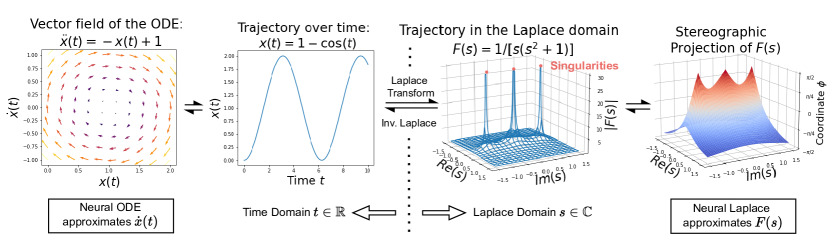
Figure 1: Comparison between Neural Laplace and Neural ODE’s modeling approaches. Neural Laplace models DE solutions in the Laplace domain $F(s)$ and uses the inverse Laplace transform to generate the time solution $x(t)$ at any time in the time domain. The Laplace representation $F(s)$ can represent broader classes of DE solutions than that of an ODE. Neural Laplace further uses a stereographic projection to remove the singularities $\infty$ of $F(s)$, forming a continuous and compact domain that improves learning. In contrast, Neural ODE models $\dot{x}$ in the time domain using a stepwise numerical ODE solver to generate the time solution.

Prior works have attempted to address these limitations separately and individually, which leads to a suite of methods that are often incompatible with each other. Whilst there has been some work on adapting Neural ODE to model DDEs specifically (Anumasa & PK, 2021; Zhu et al., 2020), their specialized architecture and inference methods rule out the possibility to model other classes of DEs (e.g. IDE or forced ODE). Similarly, the works on modeling stiff ODEs have proposed alternative system parameterizations that are invalid for other classes of DEs (Biloš et al., 2021).

In this work, we take a holistic approach and propose a unified framework, Neural Laplace, to learn a broad range of DEs (Table 1) which have vast applications (Appendix A). Importantly, Neural Laplace does not require the user to specify the class of DE a priori (e.g. choosing between ODE and DDE). Rather with the same network, the appropriate class of DE will be determined implicitly in a data-driven way. This significantly extends the flexibility and modeling capability of the existing works.

Unlike the existing works in Neural ODE, which solve the ODE in the time domain (Equation 1), Neural Laplace leverages the Laplace transform and models the DE in the Laplace domain (Figure 1). This brings two immediate advantages. First, many classes of DEs including DDE and IDE can be easily represented and solved in the Laplace domain (Cooke, 1963; Yi et al., 2006; Pospisil & Jaros, 2016; Cimen & Uncu, 2020; Smith, 1997). Secondly, Neural Laplace bypasses the numerical ODE solver and constructs the time solution $\mathbf{x}(t)$ with global summations of complex exponentials (through the inverse Laplace transform, Figure 2). It is worth highlighting that the conventional Laplace transform method is used to solve a known DE with an analytical form; yet Neural Laplace focuses on learning an unknown DE with neural networks and leverages the Laplace transform as a component.

Contributions. We propose Neural Laplace—a unified framework of learning diverse classes of DEs for modeling dynamical systems. Unlike Neural ODE, Neural Laplace uses neural networks to approximate the DEs in the Laplace domain, which allows it to model general DEs. To facilitate learning and generalization in the Laplace domain, Neural Laplace leverages the stereographic projection of the complex plane on the Reimann sphere. Empirically, we show on diverse datasets that Neural Laplace is able to accurately predict DE dynamics with complex history dependencies, abrupt changes, and piecewise external forces, where Neural ODE falls short.

We have released a PyTorch (Paszke et al., 2017) implementation of Neural Laplace, including GPU implementations of several ILT algorithms. The code for this is at https://github.com/samholt/NeuralLaplace.

2 Related work

Table 2: Comparison with existing works. Neural Laplace is a unified framework of learning diverse classes of DEs.

		Quantity	Initial	Representable classes of DEs
Method	Reference	Modeled	Condition	ODE	DDE	IDE	Forced DE	Stiff DE
Neural ODE	Chen et al. (2018)	$\dot{\mathbf{x}}(t)$	$\mathbf{x}(0)$	✓	✗	✗	✗	✗
ANODE	Dupont et al. (2019)	$\dot{\mathbf{x}}(t),\dot{\mathbf{z}}(t)$	$\mathbf{x}(0),\mathbf{0}$	✓	✗	✗	✗	✗
Latent ODE	Rubanova et al. (2019)	$\dot{\mathbf{z}}(t)$	$\mathbf{z}(0)$	✓	✗	✗	✗	✗
ODE2VAE	Yildiz et al. (2019)	$\dot{\mathbf{x}}(t),\ddot{\mathbf{x}}(t)$	$\mathbf{x}(0),\dot{\mathbf{x}}(0)$	✓	✗	✗	✗	✗
Neural DDE	Zhu et al. (2020)	$\dot{\mathbf{x}}(t)$	$\mathbf{x}(t),t\leq 0$	✗	✓	✗	✗	✗
Neural Flow	Biloš et al. (2021)	$\mathbf{x}(t)$	$\mathbf{x}(0)$	✓	✗	✗	✗	✓
Neural IM	Gwak et al. (2020)	$\dot{\mathbf{x}}(t)$	$\mathbf{x}(0)$	✓	✗	✗	✓	✗
Neural Laplace	This work	$\mathbf{F}(\mathbf{s})$	$\mathbf{p}$	✓	✓	✓	✓	✓

Table 2 summarizes the key features of the related works and compares them with Neural Laplace.

Neural ODEs model temporal dynamics with ODEs learned by neural networks (Chen et al., 2018). As a result, Neural ODE inherits the fundamental limitations of ODEs. Specifically, the temporal dynamics $\dot{\mathbf{x}}(t)$ only depends on the current state $\mathbf{x}(t)$ but not on the history. This puts a theoretical limit on the complexity of the trajectories that ODEs can model, and leads to practical consequences (e.g. ODE trajectories cannot intersect). Some existing works mitigate this issue by explicitly augmenting the state space (Dupont et al., 2019), introducing latent variables (Rubanova et al., 2019) or higher order terms (Yildiz et al., 2019). However, they still operate in the ODE framework and cannot model broader classes of DEs. Recently, Zhu et al. (2020) proposes a specialized neural architecture to learn a DDE, but the method is unable to learn the more complex IDE and often suffers from numerical instability. Kidger et al. (2020b) proposes to learn history dependency with controlled DEs, but the method requires the trajectory to be twice-differentiable (thus not applicable to systems with abrupt changes).

Another limitation of Neural ODE and extensions is that they struggle to model certain types of dynamics due to numerical instability. This is because Neural ODE relies on a numerical ODE solver (Equation 1) to predict the trajectory (forward pass) and to compute the network gradients (backward pass). Two common scenarios where standard numerical ODE solvers fail are (1) systems with piecewise external forcing or abrupt changes (i.e. discontinuities) and (2) stiff ODEs (Ghosh et al., 2020), both are common in engineering and biological systems (Schiff, 1999). Some existing works address this limitation by using more powerful numerical solvers. Specifically, when modelling stiff systems, Neural ODE requires special treatment in its computation: either using a very small step size or a specialized IVP numerical solver (Kim et al., 2021). Both lead to a substantial increase in computation cost. However, Neural Laplace does not require special treatment or significant increase in computation for stiff systems. Biloš et al. (2021) proposes to model the trajectory $\mathbf{x}(t)$ directly with a neural network, removing the need to use numerical solvers. However, their method cannot model broader classes of DEs or trajectories with abrupt changes. Jia & Benson (2019) propose methods that specifically deal with changing external forcing functions, but their proposals are not applicable to other DDEs and IDEs.

Furthermore, the Laplace transform has been used to construct input feature filters in the context of scale space theory (Lindeberg & Fagerström, 1996; Lindeberg, 2022).

3 Problem and Background

Notation. For a system with $D\in\mathbb{N}^{+}$ dimensions, the state of dimension $d$ at time $t$ is denoted as $x_{d}(t),\forall d=1,\dots,D,\forall t\in\mathbb{R}$. We elaborate that the trajectory $x_{d}:\mathbb{R}\to\mathbb{R}$ is a function of time, whereas the state $x_{d}(t)\in\mathbb{R},\forall t\in\mathbb{R}$ is a point on the trajectory. Thus the state vector is $\mathbf{x}(t):=[x_{1}(t),\dots,x_{D}(t)]^{T}\in\mathbb{R}^{D}$ and the vector-valued trajectory is $\mathbf{x}:=[x_{1},\dots,x_{D}]$. The state observations are made at discrete times of $t\in\mathcal{T}=\{t_{1},t_{2},\dots,T\}$.

Laplace Transform. The Laplace transform of trajectory $\mathbf{x}$ is defined as (Schiff, 1999)

$$\mathbf{F}(\mathbf{s})=\mathcal{L}\{\mathbf{x}\}(\mathbf{s})=\int_{0}^{\infty}e^{-\mathbf{s}t}\mathbf{x}(t)dt,$$ (2)

where $\mathbf{s}\in\mathbb{C}^{d}$ is a vector of complex numbers and $\mathbf{F}(\mathbf{s})\in\mathbb{C}^{d}$ is called the Laplace representation. The $\mathbf{F}(\mathbf{s})$ may have singularities, i.e. points where $\mathbf{F}(\mathbf{s})\to\mathbf{\infty}$ for one component (Schiff, 1999). Importantly, the Laplace transform is well-defined for trajectories that are piecewise continuous, i.e. having a finite number of isolated and finite discontinuities (Poularikas, 2018). This property allows a learned Laplace representation to model a larger class of DE solutions, compared to the consistently smooth ODE solutions given by Neural ODE and variants (Dupont et al., 2019).

Inverse Laplace Transform. The inverse Laplace transform (ILT) is defined as

$$\hat{\mathbf{x}}(t)=\mathcal{L}^{-1}\{\mathbf{F}(\mathbf{s})\}(t)=\frac{1}{2\pi i}\int_{\sigma-i\infty}^{\sigma+i\infty}\mathbf{F}(\mathbf{s})e^{\mathbf{s}t}d\mathbf{s},$$ (3)

where the integral refers to the Bromwich contour integral in $\mathbb{C}^{d}$ with the contour $\sigma>0$ chosen such that all the singularities of $\mathbf{F}(\mathbf{s})$ are to the left of it (Schiff, 1999). Many algorithms have been developed to numerically evaluate Equation 3. On a high level, they involve two steps: (Dubner & Abate, 1968; De Hoog et al., 1982; Kuhlman, 2013).

$$\mathcal{Q}(t) =\text{ILT-Query}(t)$$ (4)

$$\hat{\mathbf{x}}(t) =\text{ILT-Compute}\big{(}\{\mathbf{F}(\mathbf{s})|\mathbf{s}\in\mathcal{Q}(t)\}\big{)}$$ (5)

To evaluate $\mathbf{x}(t)$ on time points $t\in\mathcal{T}\subset\mathbb{R}$, the algorithms first construct a set of query points $\mathbf{s}\in\mathcal{Q}(\mathcal{T})\subset\mathbb{C}$ (Appendix B). They then compute $\hat{\mathbf{x}}(t)$ using the $\mathbf{F}(\mathbf{s})$ evaluated on these points. The number of query points scales linearly with the number of time points, i.e. $|\mathcal{Q}(\mathcal{T})|=b|\mathcal{T}|$, where the constant $b>1$, denotes the number of reconstruction terms per time point and is specific to the algorithm. Importantly, the computation complexity of ILT only depends on the number of time points, but not their values (e.g. ILT for $t=0$ and $t=100$ requires the same amount of computation). The vast majority of ILT algorithms are differentiable with respect to $\mathbf{F}(\mathbf{s})$, which allows the gradients to be back propagated through the ILT transform. We further discuss the selected ILT in Section 4 and Appendix B.

Intuitively, the inverse Laplace transform (ILT) (Equation 3) reconstructs the time solution with the basis functions of complex exponentials $e^{\mathbf{s}t}$, which exhibit a mixture of sinusoidal and exponential components (Schiff, 1999; Smith, 1997; Kuhlman, 2013). Figure 2 shows an illustration of these basis function representations.

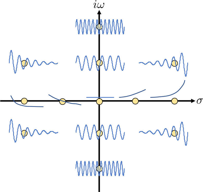
Figure 2: Individual pole points, $s=\sigma+i\omega$ and their time complex exponential reconstructions in blue, illustrated for one dimension of the $s$-domain. $\omega$ is the frequency along the imaginary axis, and $\sigma$ the real component. The complex frequency and its complex conjugate, mean the representation is symmetrical about the real axis $\sigma$. Also the Laplace transform can be seen as a complex generalisation of the Fourier transform, as we get the Fourier transform when $\sigma=0$, i.e. the imaginary axis in our Laplace representation.

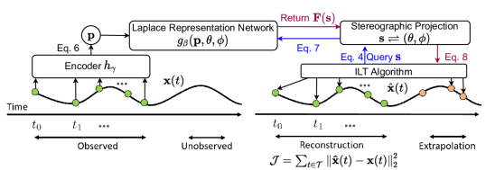
Figure 3: Block diagram of Neural Laplace. The query points $\mathbf{s}$ are given by the ILT algorithm based on the time points to reconstruct or extrapolate. The gradients can be back-propagated through the ILT algorithm and stereographic projection to train networks $h_{\gamma}$ and $g_{\beta}$.

Solving DEs in the Laplace domain. A key application of the Laplace transform is to solve broad classes of DEs, including the ones presented in Table 1 (Podlubny, 1997; Yousef & Ismail, 2018; Yi et al., 2006; Kexue & Jigen, 2011). Due to the Laplace derivative theorem (Schiff, 1999), the Laplace transform can convert a DE into an algebraic equation even when the DE contains historical states $\mathbf{x}(t-\tau)$ (as in DDE), integration terms $\int_{0}^{t}\mathbf{h}(\tau,\mathbf{x}(\tau))d\tau$ (as in IDE) or piecewise continuous terms (as in Forced ODE). It also applies to coupled DEs and can allow decoupled solutions to coupled DEs for dynamical systems (Åström & Murray, 2010). The resulting algebraic equation can either be solved analytically or numerically to obtain the solution of the DE, $\mathbf{F}(\mathbf{s})$, in the Laplace domain. Finally, one can obtain the time solution $\mathbf{x}(t)$ by applying the ILT on $\mathbf{F}(\mathbf{s})$. As we will show in the next Section, this approach of solving general DEs serves as the foundation of Neural Laplace.

There also exist numerical simulation techniques in the Laplace domain, the Laplace Transform Boundary Element (LTBE) as a numerical method for solving diffusion-type PDEs (Kuhlman, 2013; Moridis & Reddel, 1991; Moridis, 1992; Crann, 2005) and the Laplace Transform Finite Difference (LTFD) for simulation of single-phase compressible liquid flow through porous media (Moridis & Reddell, 1991; Moridis et al., 1994; Zahra et al., 2017).

4 Method

Overview of Neural Laplace. The Neural Laplace architecture involves three main components: 1. an encoder that learns to infer and represent the initial condition of the trajectory, 2. a Laplace representation network that learns to represent the solutions of DEs in the Laplace domain, and 3. an ILT algorithm that converts the Laplace representation back to the time domain. The block diagram is shown in Figure 3. We now discuss each component.

Learning to represent initial conditions. The solution of a DE depends on the initial condition of the trajectory. Different classes of DEs have different types of initial conditions. For a first-order ODE (e.g. Neural ODE), it is simply $\mathbf{x}(0)$. For a second-order ODE, it is the vector $(\mathbf{x}(0),\dot{\mathbf{x}}(0))$. And for a DDE with delay $\tau$, it is the function values $\mathbf{x}(t)$, $\forall-\tau\leq t\leq 0$. Note that we only observe the trajectories but do not know the class of DE that generates the data. Hence, we need to infer the appropriate initial condition, which implicitly determines the class of DE. To achieve this goal, Neural Laplace uses an encoder network to learn a representation of the initial condition. We highlight that the observations encoded can be at irregular times.

$$\mathbf{p}=h_{\gamma}((\mathbf{x}(t_{1}),t_{1}),(\mathbf{x}(t_{2}),t_{2}),\ldots,(\mathbf{x}(T),T))$$ (6)

The vector $\mathbf{p}\in\mathbb{R}^{K}$ is the learned initial condition representation, where $K\geq D$ is a hyper-parameter. The encoder $h$ has trainable weights $\gamma$. Neural Laplace is agnostic to the exact choice of encoder architecture. In the experiments, we use the reverse time gated recurrent unit, similar to Chen et al. (2018), for a fair comparison with the benchmarks.

Learning DE solutions in the Laplace domain. Given the initial condition representation $\mathbf{p}$, we need to learn a function ${l}:\mathbb{R}^{K}\times\mathbb{C}^{b}\to\mathbb{C}^{D}$ that models the Laplace representation of the DE solution, i.e. $\mathbf{F}(\mathbf{s})=l(\mathbf{p},\mathbf{s})$. However, the Laplace representation $\mathbf{F}(\mathbf{s})$ often involves singularities (Schiff, 1999), which are difficult for neural networks to approximate or represent (Baker & Patil, 1998). We instead propose to use a stereographic projection $(\theta,\phi)=u(s)$ to translate any complex number $s\in\mathbb{C}$ into a coordinate on the Riemann Sphere $(\theta,\phi)\in\mathcal{D}=(-{\pi},{\pi})\times(-\frac{\pi}{2},\frac{\pi}{2})$ (Rudin, 1987), i.e.

$$u(s)=\left(\arctan\left(\frac{\imaginary(s)}{\real(s)}\right),\arcsin\left(\frac{|s|^{2}-1}{|s|^{2}+1}\right)\right)$$ (7)

The inverse transform, $v:\mathcal{D}\rightarrow\mathbb{C}$, is given as

$$s=v(\theta,\phi)=\tan\left(\frac{\phi}{2}+\frac{\pi}{4}\right)e^{i\theta}$$ (8)

This produces desirable geometrical properties, that a complex point at $\infty$ is the north pole of the sphere $\phi=\frac{\pi}{2},\forall\theta$ (Rudin, 1987). With the stereographic projection, we introduce a feed-forward neural network $g$ to learn the Laplace representation of the DE solution.

$$\mathbf{F}(\mathbf{s})=v\Big{(}g_{\beta}\big{(}\mathbf{p},u(\mathbf{s})\big{)}\Big{)},$$ (9)

where projections $u$ and $v$ are defined in Equations 7 and 8 respectively, the vector $\mathbf{p}$ is the output of the encoder (Equation 6), and $\beta$ is the trainable weights. Here the neural network’s inputs and outputs are the coordinates on the Riemann Sphere, which is bounded and free from singularities. Empirically this aids learning and generalization, demonstrating that it can reduce the test RMSE dramatically compared to learning without the map (Section 5.2). The improved smoothness with the singularity mapping is shown in Figure 1, and geometry in Figure 4, for the stereographic projection map of Equation 7. A nice example of this map is the function of $1/s$, which corresponds to a rotation of the Riemann-sphere $180^{\circ}$ about the real axis. Therefore a representation of $1/s$ under this transformation becomes the map $\theta,\phi\mapsto-\theta,-\phi$ (Rudin, 1987).

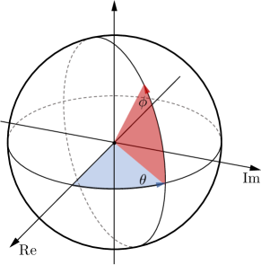
Figure 4: Geometry of the Riemann sphere map for a complex number $\mathbb{C}$ into a spherical co-ordinate representation of $\theta,\phi$.

Inverse Laplace transform. After obtaining the Laplace representation $\mathbf{F}(\mathbf{s})$ from Equation 9, we compute the predicted or reconstructed state values $\hat{\mathbf{x}}(t)$ using the ILT. We highlight that we can evaluate $\hat{\mathbf{x}}(t)$ at any time $t\in\mathbb{R}$ as the Laplace representation is independent of time once learnt. In practice, we use the well-known ILT Fourier series inverse algorithm (ILT-FSI), which can obtain the most general time solutions whilst remaining numerically stable (Dubner & Abate, 1968; De Hoog et al., 1982; Kuhlman, 2013). In Appendix B, we provide more details of the ILT-FSI and comparisons with other ILT algorithms.

We note that numerically estimating the LT on the observations $x(t)$ only gives $\mathbf{F}(\mathbf{s})$ on a finite set, $\forall\mathbf{s}\in\mathcal{U}\subset\mathbb{C}$, where $\mathcal{U}$ is determined by the observation times. Thus, this cannot generalize for extrapolation or interpolation. Whereas Neural Laplace learns $\mathbf{F}(\mathbf{s}),\forall\mathbf{s}\in\mathbb{C}$ on the entire complex domain $\mathbb{C}$.

Loss function. Neural Laplace is trained end-to-end using the mean squared error loss,

$$\mathcal{J}=\sum_{t\in\mathcal{T}}\left\|\mathbf{\hat{x}}(t)-\mathbf{x}(t)\right\|_{2}^{2},$$ (10)

where $\mathbf{\hat{x}}(t)$ is the reconstructed trajectory (Equation 5). We minimize the above loss function $\mathcal{J}$ to learn the encoder $h_{\gamma}$ and the Laplace representation network $g_{\beta}$. This training is summarized in Algorithm 1. We can also constrain the ILT reconstruction frequencies with a low pass filter, smoothing the reconstructed signal, and we empirically show a toy noise removal task of this in Appendix C.

Algorithm 1 Neural Laplace Training Procedure

  Input: Observed trajectory $\mathbf{x}(t),t\in\mathcal{T}$

  Input: Training iterations $I$

  for $i\in 1:I$ do

     $\mathbf{p}=h_{\gamma}\big{(}\{\mathbf{x}(t)|t\in\mathcal{T}\}\big{)}$ Eq. 6

     for $t\in\mathcal{T}$ do

        $\mathcal{Q}=\text{ILT-Query}(t)$ Eq. 4

        for $s\in\mathcal{Q}$ do

           $\mathbf{F}(\mathbf{s})=v\Big{(}g_{\beta}\big{(}\mathbf{p},u(\mathbf{s})\big{)}\Big{)}$ Eq. 9

        end for

        $\hat{\mathbf{x}}(t)=\text{ILT-Compute}\big{(}\{\mathbf{F}(\mathbf{s})|\mathbf{s}\in\mathcal{Q}\}\big{)}$ Eq. 5

     end for

     $\mathcal{J}=\sum_{t\in\mathcal{T}}\left\|\mathbf{\hat{x}}(t)-\mathbf{x}(t)\right\|_{2}^{2}$ Eq. 10

     Compute gradients of $\mathcal{J}$ via back propagation.

     Update neural network weights $\gamma$ and $\beta$.

  end for

  Output: the trained neural networks $h_{\gamma}$ and $g_{\beta}$

Table 3: Each DE system we use for comparison against the benchmarks, and their properties for comparison.

System	Piecewise	Discontinuous	Integro	Delay	Stiff	Periodic
	DE	differential	DE	DE	solutions	solutions
Spiral DDE	✓	✓	✗	✓	✗	✗
Lotka-Volterra DDE	✓	✓	✗	✓	✗	✗
Mackey–Glass DDE	✓	✓	✗	✓	✗	✗
Stiff Van der Pol Oscillator DE	✗	✓	✗	✗	✓	✓
ODE with piecewise forcing function	✓	✗	✗	✗	✗	✗
Integro DE	✗	✗	✓	✗	✗	✗

Comparison with Neural ODE. Here we articulate the three main differences between Neural Laplace and Neural ODE. (1) The encoders of these two frameworks serves different purposes. The Neural ODE encoder is tasked to infer the initial condition $\mathbf{x}(0)$ when it is observed with noise or unobserved (e.g. measurement starts at $t>0$). On the other hand, the Neural Laplace encoder needs to learn an appropriate representation of the initial condition and implicitly decide the class of DE to use. The representation $\mathbf{p}$ may include more information than $\mathbf{x}(0)$. (2) Neural ODE uses a neural network to approximate $\dot{\mathbf{x}}(t)$ while Neural Laplace uses a neural network to approximate $\mathbf{F}(s)$ after the stereographic projection. As a result, Neural ODE can only model twice-differentiable trajectories $\mathbf{x}(t)$ while Neural Laplace can model non-smooth trajectories. (3) Neural ODE uses numerical IVP solvers while Neural Laplace uses ILT algorithms. The ILT algorithms can handle stiff ODEs and piecewise forcing functions, where most numerical IVP solvers fail (Biloš et al., 2021). Furthermore, the time complexity of ILT for predicting $\mathbf{x}(t)$ does not depend on $t$, while numerical IVP solvers do. This brings computational benefits to Neural Laplace when the application involves a long time horizon.

5 Experiments

We evaluate Neural Laplace on a broad range of dynamical systems arising from engineering and natural sciences. These systems are governed by different classes of DEs. We show that Neural Laplace is able to model and predict these systems better than the ODE based methods.

Benchmarks. We compare against the standard and augmented Neural ODE (NODE, and ANODE respectively) with an input fixed initial condition (Dupont et al., 2019; Chen et al., 2018). We also compare with ODE models with an encoder-decoder architecture: Latent ODE with an ODE-RNN encoder (Rubanova et al., 2019), Neural Flows (NF) Coupling, and Neural Flows ResNet (Biloš et al., 2021). To ensure a fair comparison, we set the number of hidden units per layer such that all models have roughly the same number of total parameters. Further details of hyperparameters and implementation details are in Appendix D.

Evaluation. To test whether the models are able to accurately uncover the temporal dynamics, we evaluate their accuracy in predicting the future states of the system, i.e. the root mean square error (RMSE). We also evaluate the model’s ability to capture the state space distribution $P(\mathbf{x}(t))$ by calculating the conditional mutual information (CMI) between the true and the predicted distributions conditioning on the initial value distribution . We split each sampled trajectory into two equal parts $[0,\frac{T}{2}]$, $[\frac{T}{2},T]$, encoding the first half and predicting the second half. For each dataset equation we sample $1,000$ trajectories of $200$ time points in the interval of $t\in[0,20]$, with each sampled from a different initial condition giving rise to a unique trajectory defined by the same differential equation system. We divide the trajectories into a train-validation-test split of $80:10:10$, for training, hyperparameter tuning, and evaluation respectively. See Appendix E for details on how we sampled each DE system.

Dynamical systems for comparison. We selected a broad range of dynamical systems from applied sciences, and each have unique properties of interest, see Table 3 for a comparison. The systems are detailed as follows.

Spiral DDE, (Zhu et al., 2020) these are common in healthcare and biological systems, for example cardiac tissue models (Moreira Gomes et al., 2019), biological networks (Glass et al., 2021) and modelling gene dynamics (Verdugo & Rand, 2007).

$$\begin{split}\mathbf{\dot{x}}(t)=\mathbf{A}\tanh(\mathbf{x}(t)+\mathbf{x}(t-\tau)),\quad t>0\\ \end{split}$$ (11)

with the time delay $\tau=2.5$ and $\mathbf{A}\in\mathbb{R}^{2\times 2}$ a constant matrix. We generate trajectories by sampling from a grid for each state dimension of the fixed initial history $\mathbf{x}(t),t\leq 0$ in the interval $[-2,2]$.

Table 4: Test RMSE for datasets analyzed. Best results bolded. Averaged over $5$ runs.

	Spiral	Lotka-Volterra	Mackey-Glass	Stiff Van der	ODE piecewise	Integro
Method	DDE	DDE	DDE	Pol Oscillator DE	forcing function	DE
NODE	.0389 $\pm$ .0029	.3102 $\pm$ .0151	.8225 $\pm$ .0403	.2833 $\pm$ .0032	.2274 $\pm$ .0298	.0730 $\pm$ .0016
ANODE	.0365 $\pm$ .0011	.2930 $\pm$ .0239	.8214 $\pm$ .0415	.2444 $\pm$ .0167	.0644 $\pm$ .0211	.0036 $\pm$ .0003
Latent ODE	.0481 $\pm$ .0033	.2182 $\pm$ .0153	.0385 $\pm$ .0217	.1932 $\pm$ .0154	.1401 $\pm$ .0457	.0109 $\pm$ .0009
NF Coupling	.6938 $\pm$ .1036	.7266 $\pm$ .0310	.0539 $\pm$ .0181	.1829 $\pm$ .0209	.0752 $\pm$ .0052	.0042 $\pm$ .0013
NF ResNet	.1905 $\pm$ .0479	.2257 $\pm$ .0608	.0350 $\pm$ .0223	.1468 $\pm$ .0396	.0399 $\pm$ .0119	.0027 $\pm$ .0004
Neural Laplace	.0331 $\pm$ .0023	.0475 $\pm$ .0061	.0282 $\pm$ .0246	.1314 $\pm$ .0218	.0035 $\pm$ .0004	.0014 $\pm$ .0005

Lotka-Volterra DDE (Bahar & Mao, 2004), also known as the predator-prey equations, are fundamental to ecology and population modeling.

$$\dot{x}=\frac{1}{2}x(t)(1-y(t-\tau));\quad\dot{y}=\frac{1}{2}y(t)(1-x(t-\tau))$$ (12)

We use a fixed delay of $\tau=0.1$, generating trajectories by sampling from a grid for each state dimension of the fixed initial history $\mathbf{x}(t),t\leq 0$ in the interval $[0.1,2]$, and instead sample time points in the interval of $t\in[0.1,2]$.

Mackey–Glass DDE, (Mackey & Glass, 1977), modified to exhibit long range dependencies, given the form,

$$\dot{x}=\beta\frac{x(t-\tau)}{1+x(t-\tau)^{n}}-\gamma x(t)$$ (13)

Using a fixed delay of $\tau=10,n=10,\beta=0.25,\gamma=0.1$, generating trajectories by uniformly changing the initial history to be either $-1$, or $1.1$ over the time interval of $[0,10]$ for $t<10$, as seen in Figure 5.

Stiff Van der Pol Oscillator DE, (Van der Pol & Van Der Mark, 1927), which exhibits regions of high stiffness when setting $\mu=$1,000,

$$\dot{x}=y;\quad\dot{y}=\mu(1-x^{2})y-x$$ (14)

We sample initial conditions from $x(0)\in[0.1,2],y(0)=0$.

ODE with piecewise forcing function, an ODE with a ramp loading forcing function (common in engineering applications) (Boyce et al., 2021). This exhibits piecewise DE behaviour, i.e. a different ODE in the different forcing function piecewise regions.

$$\ddot{x}+4x(t)=u(t);\quad u(t)=\begin{cases}0&\ 0<t\leq 5\\ \frac{t-5}{5}&\ 5<t\leq 10\\ 1&\ 10<t<20\\ \end{cases}\\$$ (15)

We sample initial conditions from $x(0)\in[0,0.1],\dot{x}(0)=0$.

Integro DE, Integral and differential system (Bourne, 2018).

$$\begin{split}\dot{x}+2x(t)+5\int_{0}^{t}x(t)dt&=u(t)\\ \end{split}$$ (16)

Where $u(t)$ is the Heaviside step function, sampling initial conditions from $x(0)\in[0,1]$ and sampling times in the interval of $t\in[0,4]$.

In Appendix L, we compare our method on periodic waveforms that are not governed by a standard DE. We observe Neural Laplace is better at reconstruction compared to the benchmarks in extrapolating these non-DE trajectories.

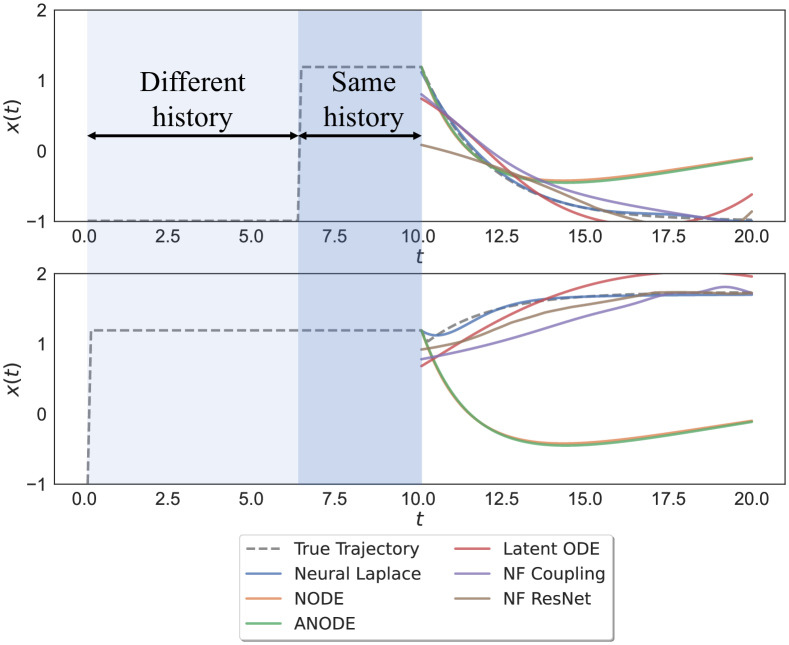
Figure 5: Two test trajectories of the Mackey Glass DDE, with benchmarks, illustrating examples where the distant history impact the future trajectory, even though momentarily they may have the same history for short times, $6\leq t\leq 10$.

5.1 Results Discussion

The RMSE for each dataset comparing against the benchmarks, are tabulated in Table 4. Neural Laplace achieves low RMSE extrapolation test error on all DE datasets analyzed. The CMI metric follows a similar pattern and is presented in Appendix F. We also observe a similar pattern on DE datasets corrupted with noise in Appendix I and on DE datasets with smaller sizes, of trajectories and observations in Appendix H. Neural Laplace is able to correctly learn the DE system using its global complex exponential basis function representation through encoding the observed trajectory into the initial condition representation for that DE system, and extrapolating forwards in time. We analyse a few typical scenarios in detail to gain a better understanding. See Appendix M for additional analysis and visualization.

Systems with long range dependency. The experiments on Mackey–Glass DDE offers insight into the model’s ability to capture long range dependencies. As illustrated in Figure 5, trajectories with the same recent history ($6\leq t\leq 10$) but different distant histories ($0\leq t<6$) evolve very differently in the future ($t>10$). Hence, successful extrapolation requires the model to keep memory from the distant past. NODE and ANODE methods fail to capture this because $x(10)$, the initial condition for the ODE to extrapolate, is the same for both trajectories—this leads to the same extrapolation (Figure 5). Latent ODE and Neural Flow methods start to encode some history dependency. However they still fail to capture the true solution, being overly smooth and unable to capture the piecewise initial history. Whereas Neural Laplace is able to correctly learn the historical dependency of the DE system. Similar patterns are observed in other systems with long range dependencies (e.g. Spiral and Lotka-Volteera DDE) and further illustrated in Appendix M.

Table 5: Neural Laplace ablation study and sensitivity analysis. RMSE is reported under different study configurations on different dynamical systems. Averaged over $5$ runs.

		Lotka-Volterra	Stiff Van der	ODE piecewise	Integro
Study	Config.	DDE	Pol Oscillator DE	forcing function	DE
Stereographic	✗	.1617 $\pm$ .0741	.1836 $\pm$ .0586	.0249 $\pm$ .0066	.0048 $\pm$ .0007
projection	✓	.0614 $\pm$ .0469	.1286 $\pm$ .0170	.0036 $\pm$ .0007	.0013 $\pm$ .0003
	1	.4416 $\pm$ .0898	.1520 $\pm$ .0240	.0036 $\pm$ .0007	.0010 $\pm$ .0002
	2	.0405 $\pm$ .0113	.1308 $\pm$ .0159	.0033 $\pm$ .0009	.0012 $\pm$ .0002
Dimensionality	4	.0427 $\pm$ .0049	.1334 $\pm$ .0103	.0038 $\pm$ .0013	.0012 $\pm$ .0003
$K$	8	.0408 $\pm$ .0134	.1294 $\pm$ .0173	.0038 $\pm$ .0004	.0010 $\pm$ .0002
	16	.0380 $\pm$ .0053	.1334 $\pm$ .0197	.0036 $\pm$ .0006	.0012 $\pm$ .0005
	32	.0398 $\pm$ .0045	.1337 $\pm$ .0203	.0032 $\pm$ .0005	.0013 $\pm$ .0003

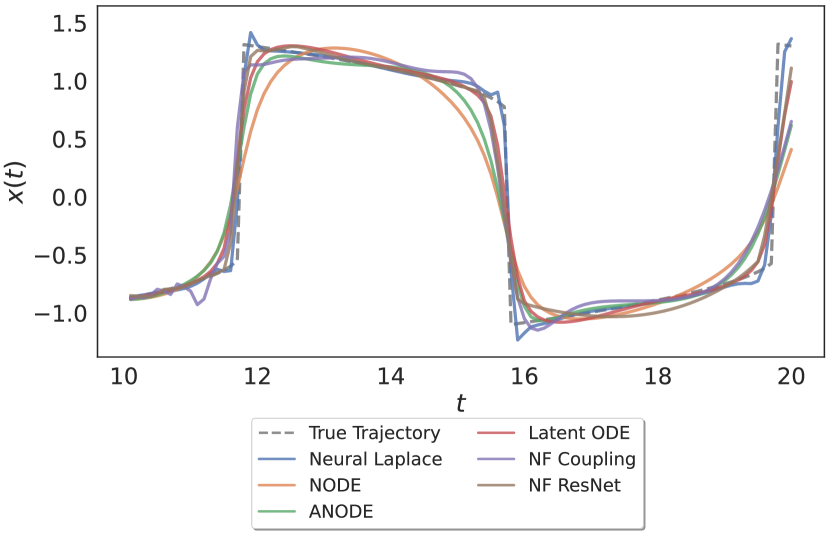
Figure 6: Test extrapolation plots with benchmarks for Stiff Van der Pol Oscillator DE. Neural Laplace is able to correctly extrapolate the DE dynamics.

Systems with abrupt changes and stiffness. The trajectory plot in Figure 6, of a test trajectory, shows that Neural Laplace is able to correctly learn the periodic stiff solution, capturing the discontinuities of the derivative of the solution and the periodicity. NODE, ANODE and Latent ODE methods, correctly capture the periodicity, however fall short in modelling the derivative discontinuities as they enforce overly smooth solutions. Neural Flow methods suffer from similar smoothness behaviour.

5.2 Ablation study and sensitivity analysis

Ablation study for stereographic projection. We investigate how useful the stereographic projection is for learning a Laplace representation of a DE system. Table 5 (top) shows the test RMSE with and without it in Neural Laplace. This demonstrates empirically that using the stereographic projection Riemann sphere map can allow us to achieve an order of magnitude reduced test RMSE. This supports our belief that the stereographic projection improves learning by inducing a more compact geometry in the Laplace domain.

Sensitivity to dimensionality $K$. In Neural Laplace, the encoded representation of the initial condition $\mathbf{p}\in\mathbb{R}^{K}$ has dimensionality $K$, a hyperparameter. We explore the sensitivity of this dimension, reporting the test RMSE in Table 5. This empirically shows that the performance is not sensitive to the exact choice of $K$, as long as it is set to a large enough value (e.g. $K\geq 2$).

5.3 Computation time and complexity

Linear forward evaluations Extrapolating to a single time point at any future time $t$ only uses a single forward evaluation in Neural Laplace’s Laplace representation model $g_{\beta}\big{(}\mathbf{p},u(\mathbf{s}))$, whereas ODE based methods (NODE, ANODE) scale poorly in number of forward evaluations when extrapolating to any increasing future time $t$, as they use numerical stepwise ODE solvers. For comparison Figure 7 (a) shows Neural Laplace can use one thousand times less NFEs when extrapolating forwards a $100$ seconds (Appendix G). However Neural Laplace does scale in NFEs linearly with the amount of time points to evaluate at, Figure 7 (b), which is the same for other integral DE methods (Biloš et al., 2021). Furthermore, Neural Laplace is empirically at least an order magnitude faster to train per epoch than ODE based methods, measuring wall clock (Appendix J), and can comparatively converge faster (Appendix K).

6 Conclusion and Future work

We have shown that through a novel geometrical construction, it is possible to learn a useful Laplace representation model for a broad range of DE systems, such as those not able to be modelled by simple ODE based models, those of delay DEs, Stiff DEs, Integro DEs and ODEs with piecewise forcing functions. Neural Laplace can model the same systems ODE based methods can as well, whilst being faster to train and evaluate, using the Inverse Laplace Transform to generate time solutions instead of using costly, DE stepwise numerical solvers. We hope this work provides a practical framework to learn a Laplace representation of a system, which is immensely useful and popular in the fields of science and engineering (Schiff, 1999).

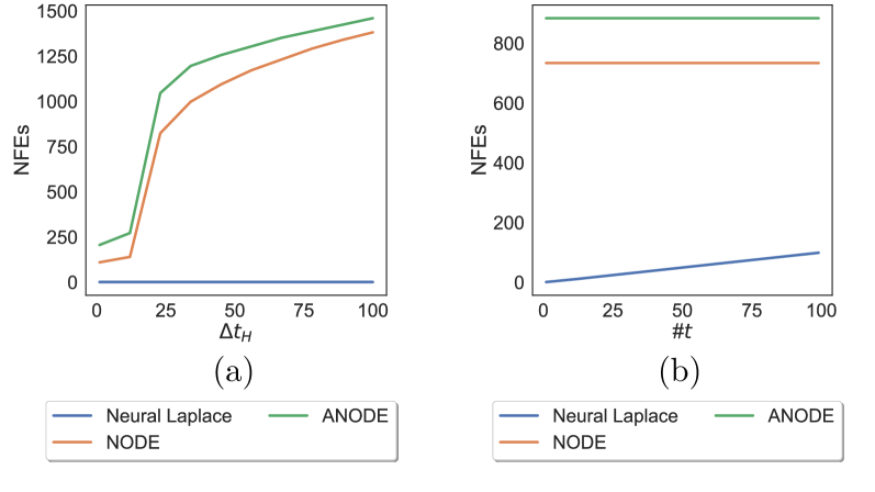
Figure 7: NFEs (a) for extrapolating to a single future time point, that is $\Delta t_{H}$ in the future, (b) for increasing the number of time points evaluated within a fixed interval of time.

In future work we wish to use the learned Laplace representation to investigate the other unique properties of this representation, such as stability analysis, limiting its frequency reconstruction terms, and using the Laplace final limit theorem (Schiff, 1999) as an additional regularizer. We note that we chose the stereographic projection because it is the simplest and most well-studied bijective map, that maps the entire complex domain to a compact domain (Rudin, 1987). Future work could include using other complex bijective maps instead. It could also be interesting to explore other integral transforms with a similar geometrical smoothness map to a compact domain, such as the Mellin transform and others (Debnath & Bhatta, 2014) that have unique properties that are advantageous to learn a representation for.

Acknowledgements

SH would like to acknowledge and thank AstraZeneca for funding. This work was additionally supported by the Office of Naval Research (ONR) and the NSF (Grant number: 1722516). Additionaly we thank Arsenii Nikolaiev for the helpful discussion. Furthemore we would like to warmly thank all the anonymous reviewers, alongside research group members of the van der Scaar lab, for their valuable input, comments and suggestions as the paper was developed. All these inputs ultimately improved this paper.

Table of supplementary materials

1. Appendix A: Applications of DEs

2. Appendix B: Inverse Laplace Transform Algorithms

3. Appendix C: Limiting Reconstruction Frequencies

4. Appendix D: Benchmark Implementation and Hyperparameters

5. Appendix E: Sampling Each DE Dataset

6. Appendix F: Capturing State Space Distribution

7. Appendix G: NFE Analysis

8. Appendix H: Sample and Observation Size Scaling

9. Appendix I: Additional Benchmark Results

10. Appendix J: Benchmark Wall Clock Times

11. Appendix K: Training Loss Plots

12. Appendix L: Extrapolating Toy Waveforms

13. Appendix M: Dataset Plots

Code. We have released a PyTorch implementation (Paszke et al., 2017), including GPU implementations of several ILT algorithms at https://github.com/samholt/NeuralLaplace. We also have a research group codebase, which can be found at https://github.com/vanderschaarlab/NeuralLaplace.

Table 6: Applications of the families of DEs captured by Neural Laplace.

Type	Applications
ODE	Dynamical systems (Teschl, 2012), Biological systems (Su et al., 2021)
DDE	Biological systems (Moreira Gomes et al., 2019; Glass et al., 2021; Verdugo & Rand, 2007), Electrodynamics (López, 2020)
IDE	Engineering (Zill, 2016), Epidemiology (Medlock, 2004), Finance (Sachs & Strauss, 2008)
Forced ODE	Control Theory (Filippov, 2013), Engineering (Boyce et al., 2021)
Stiff ODE	Engineering (Van der Pol & Van Der Mark, 1927), Chemistry (Sandu et al., 1997)

Table 7: Comparison of ILT algorithms that we considered and implemented.

ILT	Limitations on	$\mathbf{F}(\mathbf{s})$	Robust	Model	Model	Supports
	$\mathbf{x}(t)$			sinusoids	exponentials	batching
Fourier Series Inverse	None	Complex	✓	✓	✓	✓
CME	None	Complex	✓	✓	✓	✓
de Hoog	None	Complex	✗	✓	✓	✗
Fixed Tablot	No medium	Complex	✓	✗	✓	✓
	/ large frequencies
Stehfest	No oscillations,	Real part only	✗	✗	✓	✓
	no discontinuities in $\mathbf{x}(t)$

Appendix A Applications of DEs

The families of DEs that Neural Laplace can capture in Table 1 have wide applications with some of their applications listed in Table 6.

Appendix B Inverse Laplace Transform Algorithms

We use the well-known ILT Fourier series inverse algorithm (ILT-FSI), as it can obtain the most general time solutions whilst remaining numerically stable (Dubner & Abate, 1968; De Hoog et al., 1982; Kuhlman, 2013). Others (Kuhlman, 2013) have shown empirically in a review of ILT methods, ILT-FSI methods are the most robust, although we do not get the same convergence guarantees as with other well known inverse Laplace transforms, such as Tablot’s method. However these cannot represent frequencies, i.e. poles of the system that pass its restrictive deformed integral contour of Eq. 3, leading to only sufficient representation of solutions of decaying exponentials.

We implemented five inverse Laplace transform algorithms, choosing them for their good performance, somewhat ease of implementation and robustness as indicated in the review of (Kuhlman, 2013). Implemented in PyTorch (Paszke et al., 2017). They are, Fourier Series Inverse (Dubner & Abate, 1968; De Hoog et al., 1982), de Hoog (De Hoog et al., 1982), Fixed Tablot (Abate & Valko, 2004), Stehfest (Stehfest, 1970) and concetrated matrix exponentials (CME) (Horváth et al., 2020). We compare them in table 7 and in the following we explain each one, comparing each ILT to determine which one best suits our purpose of modelling arbitrary solutions. For a detailed in depth comparison and description of their properties (excluding CME) see the review of (Kuhlman, 2013). They are as follows,

Fourier Series Inverse Expands Equation 3 into an expanded Fourier transform, approximating it with the trapezoidal rule. This keeps the Bromwich contour parallel to the imaginary axis, and shifts it along the real axis, following the definition in Equation 17, i.e. $\sigma\propto\frac{1}{t}$. It is fairly easy to implement and scale to multiple dimensions. We denote $s=\sigma+i\omega$ and we can express Equation 3 as,

$$\begin{split}\mathbf{x}(t)&=\frac{1}{\pi}e^{\sigma t}\int_{0}^{\infty}\real\left\{F(s)e^{i\omega t}\right\}d\omega\\ &\approx\frac{1}{T}e^{\sigma t}\left[\frac{F(\sigma)}{2}+\sum_{k=1}^{2N}\real\left\{F\left(\sigma+\frac{ik\pi}{T}\right)e^{\frac{ik\pi t}{T}}\right\}\right]\end{split}$$ (17)

Where we approximate the first Fourier ILT, Equation 17 as a discretized version, using the trapezoidal rule with step size $\frac{\pi}{T}$ (Dubner & Abate, 1968) and evaluating $s$ at the approximation points $s_{k}=\sigma+\frac{ik\pi}{T}$ in the trapezoidal summation. We follow (Kuhlman, 2013) to set the parameters of $\sigma=\alpha-\frac{\log(\epsilon)}{T}$, with $\alpha=$1e-3, $\epsilon=10\alpha$, and the scaling parameter $T=2t$. This gives the query function,

$$\begin{split}s_{k}(t)&=\text{1e-3}-\frac{\log(\text{1e-2})}{2t}+\frac{ik\pi}{2t}\\ \mathcal{Q}(t)&=[s_{0}(t),\ldots,s_{2N}(t)]^{T}\end{split}$$ (18)

Where we model the equation with $2N+1$ reconstruction terms, setting $N=16$ in experiments, and use double point floating precision to increase the numerical precision of the ILT.

The ILT-FSI, of Equation 17 provides guarantees that we can always find the inverse from time $t:0\rightarrow\infty$, given that the singularities of the system (i.e. the points at which $F(s)\to\infty$) lie left of the contour of integration, and this puts no constraint on the imaginary frequency components we can model. Of course in practice, we often do not model time at $\infty$ and instead model up to a fixed time in the future, which then bounds the exponentially increasing system trajectories, and their associated system poles that we can model $\sigma\propto\frac{1}{t}$.

de Hoog Is an accelerated version of the Fouier ILT, defined in Equation 17. It uses a non-linear double acceleration, using Padé approximation along with a remainder term for the series (De Hoog et al., 1982). This is somewhat complicated to implement, due to the recurrence operations to represent the Padé approximation, due to this although higher precision (Kuhlman, 2013), the gradients have to propagate through many recurrence relation paths, making it slow to use in practice compared to Fourier (FSI), however more accurate when we can afford the additional time complexity.

Fixed Tablot Deforms the Bromwich contour around the negative real axis, where $\mathbf{F}(\mathbf{s})$ must not overflow as $\mathbf{s}\to-\infty$, and makes the Bromwich contour integral rapidly converge as $\mathbf{s}\to-\infty$ causes $e^{\mathbf{s}t}\to 0$ in Equation 3. We implemented the Fixed Tablot method (Abate & Valko, 2004; Talbot, 1979), which is simple to implement. However it suffers from not being able to model solutions that have large sinusoidal components and instead is optimized for modelling decaying exponential solutions. We note that whilst it can approximate some small sinusoidal components, for an adaptive time contour as in (Kuhlman, 2013), the sinusoidal components that can be represented decrease when modelling longer time trajectories, and in the limit for long time horizons, allow only representations of decaying exponentials.

Stehfest Uses a discrete version of the Post-Widder formula (Al-Shuaibi, 2001) that is an approximation for Equation 3 using a power series expansion of real part of $\mathbf{s}$. It has internal terms that alternate in sign and become large as the order of approximation is increased, and suffers from numerical precision issues for large orders of approximation. It is fairly easy to implement.

CME Concentrated matrix exponential (CME), uses a similar form to that of the Fourier Series Inverse, approximating Equation 3 with the trapezoidal rule (Horváth et al., 2020). This uses the form of,

$$\mathbf{x}(t)\approx\frac{1}{T}\sum_{k=1}^{2N}\eta_{k}F\left(\frac{\beta_{k}}{T}\right)$$ (19)

The coefficients $\eta_{k},\beta_{k}$ are determined by a complex procedure, with a numerical optimization step involved (Horváth et al., 2020). This provides a good approximation for the reconstruction and the coefficients of up to a pre-specified order can be pre-computed and cached for low complexity run time (Horváth et al., 2020). Similarly to Fourier (FSI), CMEs Bromwich contour remains parallel to the imaginary axis and is shifted along the real axis, i.e. $\sigma\propto\frac{1}{t}$. It is moderately easy to implement when using pre-computed coefficients and scale to multiple dimensions. We use $N=16$, to set the reconstruction terms.

The review author of (Kuhlman, 2013) found that for boundary element simulations the Fourier based, ILT Fourier series algorithms were the most robust and most precise. Our test comparison in Table 8 confirms this, with de Hoog being the most precise, however implementing the recurrence operation in PyTorch, causes it to perform slowly as a decoder due to the significantly more gradient operators and path length compared to that of Fourier series inverse ILT. All these discussed ILT algorithms are implemented and included in the code for this paper.

Table 8: Inverse Laplace Transform algorithms compared against the numerical inversion $F(s)=\frac{s}{s^{2}+1}$ to it’s analytic time function of $x(t)=\cos(t)$. We evaluate for the times $t\in[0,10.0]$ for 1,000 linearly spaced time points. We fix each algorithm to use $2N+1$ reconstruction terms per time point, with $N=16$.

ILT	$\text{RMSE}(x(t),\hat{x}(t))$	Forward pass
Algorithm		time per $t$ ($\mu s$)
Fourier (FSI)	0.0171	2.6331
Tablot	0.4365	3.7520
Stehfest	0.2842	0.5839
de Hoog	7.056E-10	20.3071
CME	0.0069	1.8759

Furthermore Table 8 shows that CME is also competitive compared to Fourier (FSI) ILT algorithm. However we empirically observe in Figure 8, that Neural Laplace converges faster when using the Fourier (FSI) ILT algorithm compared to using the CME ILT algorithm.

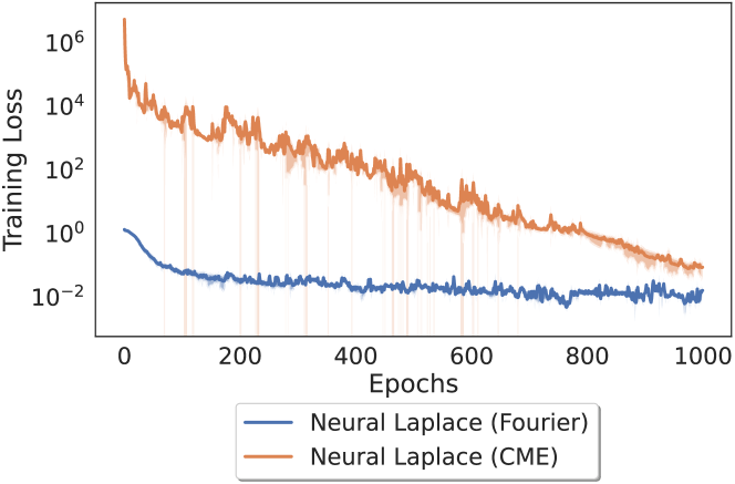
Figure 8: Training loss for Lotka-Volterra DDE. Averaged over 3 runs.

Appendix C Limiting reconstruction frequencies

We consider a toy example of a true signal with high frequency noise as,

$$\begin{split}y_{\text{uncorrupted}}&=\sin(t)+\sin(2t)\\ y_{\text{corrupted}}&=y_{\text{uncorrupted}}+0.5\sin(11t)\end{split}$$ (20)

We can explicitly filter our reconstruction frequencies before doing the ILT in Neural Laplace. Here we use a low pass filter, and only allow reconstruction of frequencies below $3$ Hz. We do this by constraining the maximum value of $\phi$ that we can learn, by not allowing any $s$ greater than $|3|$ in the s-domain representation, using Equation 7 to set $\phi$. This also limits the exponentials that we can learn as well. Empirically when we do this we can recover the true noise free signal, when training a Neural Laplace model on the corrupted signal. This is advantageous as the true signal is recovered and it was never observed, although we added the prior information that frequencies above a certain threshold are noise and should be disregarded. A plot of this toy example can be seen in Figure 9.

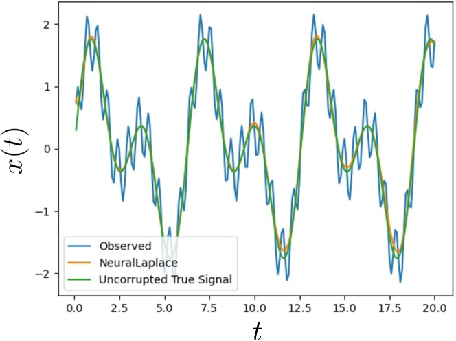
Figure 9: We can limit the frequency that our Neural Laplace model can learn, by applying a low pass frequency filter, to only be able to reconstruct frequencies of interest if we know the frequency range to expect, ideally below the observed noise frequency.

Appendix D Benchmark implementation and hyperparameters

Table 9: Benchmarks implemented and their number of parameters for each model.

Method	# Parameters
NODE	17,025
ANODE	17,282
Latent ODE	18,565
NF coupling	18,307
NF ResNet	18,307
Neural Laplace	17,194

For our benchmarks, we tune all methods to have the same number of approximate parameters, as seen in Table 9, to ensure fair comparison for any gains in modelling complexity. We also set the latent dimension if one exists for each method to be 2, (although we show in Section 5.2, that Neural Laplace can benefit with a latent dimension greater than 2). To aid the ILT numerical stability, we train and evaluate all models and all data with double point floating precision, as is recommended when using ILTs (Kuhlman, 2013). We use the Adam optimizer (Kingma & Ba, 2017) with a learning rate of 1e-3, and batch size of 128. When training we use early stopping using the validation data set with a patience of 100, training for 1,000 epochs unless otherwise stated. These benchmarks are:

Neural ODE (Chen et al., 2018), using their code and implementation provided, setting the ODE function $\mathbf{f}(t,\mathbf{x}(t))$ to a 3 layer Multilayer perceptron (MLP), of 128 units, with $\tanh$ activation functions. As NODE does not have an encoder, we set the initial value to the last observed trajectory value at the last observed time. To allow for fair comparison we use the semi-norm trick for faster back propagation (Kidger et al., 2020a), and use the ’euler’ solver unless otherwise stated. Using the reconstruction MSE for training.

Augmented Neural ODE (Dupont et al., 2019), we also use their implementation provided, setting the ODE function $\mathbf{f}(t,\mathbf{x}(t))$ to be a 3 layer MLP, of 128 units, with $\tanh$ activation functions, with an additional augmented dimension of zeros. Again ANODE does not have an encoder, so we set the initial value to the last observed trajectory value at the last observed time, and also use the semi-norm trick, and use the ’euler’ solver unless otherwise stated. Additionally we use the reconstruction MSE for training.

Latent ODE (Rubanova et al., 2019), which uses an ODE-RNN encoder and an ODE model decoder. We use their code provided, setting the units to be 40 for the GRU and ODE function $\mathbf{f}(t,\mathbf{x}(t))$ net, with $\tanh$ activation, which uses the ’dopri5’ solver. We also use their reconstruction variational loss function for training.

Neural Flows (Biloš et al., 2021), we use their code provided, with the coupling flow using 31 units, and the ResNet flow using 26 units. Again we use their reconstruction variational loss function for training.

Neural Laplace This paper, uses a GRU encoder $h_{\gamma}$ (Cho et al., 2014), with 2 layers, with 21 units, with a linear layer on the final hidden state which outputs the latent initial condition $\mathbf{p}$. For the Laplace representation model, $g_{\beta}$ we use a 3 layer MLP with 42 units, with $\tanh$ activations. We use $\tanh$ on the output to constrain the output domain to be $(\theta,\phi)\in\mathcal{D}=(-{\pi},{\pi})\times(-\frac{\pi}{2},\frac{\pi}{2})$ for each observation dimension. For a given trajectory we encode it into $\mathbf{p}$ and concatenate with $u(\mathbf{s})$ as input to $g_{\beta}$, i.e. $g_{\beta}\big{(}\mathbf{p},u(\mathbf{s}))$.

Table 10: Test conditional mutual information (CMI) between the predicted extrapolation to that of the ground truth extrapolation. Best results are bolded. Averaged over $5$ runs. Higher mutual information score is best.

	Mackey-Glass	Lotka-Volterra	Stiff Van de
Method	DDE	DDE	Pol Oscillator DE
NODE	0.2899 $\pm$ 0.0478	3.2479 $\pm$ 0.0910	2.8658 $\pm$ 0.0142
ANODE	0.2865 $\pm$ 0.0502	3.2398 $\pm$ 0.0560	2.9679 $\pm$ 0.1022
Latent ODE	1.3736 $\pm$ 0.1246	3.3908 $\pm$ 0.0357	2.7692 $\pm$ 0.1446
NF Coupling	1.5569 $\pm$ 0.1871	2.1696 $\pm$ 0.5000	2.7183 $\pm$ 0.1766
NF ResNet	1.5730 $\pm$ 0.1615	3.4854 $\pm$ 0.1551	3.0832 $\pm$ 0.1435
Neural Laplace	1.6011 $\pm$ 0.1571	3.7913 $\pm$ 0.0359	3.3224 $\pm$ 0.1157

Appendix E Sampling each DE dataset

We test the benchmarks for extrapolation and split each sampled trajectory into two equal parts $[0,\frac{T}{2}]$, $[\frac{T}{2},T]$, encoding the first half and predicting the second half. For each dataset equation we sample 1,000 trajectories, each with a different initial condition giving rise to a different and unique trajectory defined by the same differential equation system. We use a train-validation-test split of 80:10:10, and train each model for 1,000 epochs with a learning rate of 1e-3 and unless otherwise specified we sample each system in the interval of $t\in[0,20]$ for 200 time points linearly. For each sequential experiment for the same method we set a different random seed. We also use the training set to normalize the train, val and test set.

To sample the delay DE systems, we use a delay differential equation solver of Zulko (2019), to sample the Spiral DDE, Lotka-Volterra DDE, and Mackey–Glass DDE data sets. We use 2,000 samples in the DDE solver and then subsampled the generated trajectories to 200 time points in the time interval defined for the dataset. The Mackey-Glass DDE dataset was sampled in the time interval $[0,100]$ and then scaled down to $[0,20]$ for equal comparison with the benchmarks. Trajectories of it can be seen in Figure 5, with benchmarks trained for 50 epochs. To sample the stiff DEs, that of the Stiff Van der Pol Oscillator we use the stiff DE solver of ’ode15s’ (Shampine & Reichelt, 1997), we sampled for a given initial condition between the times of 0 to 4000, generating 200 time points for each trajectory. Once the trajectories were generated we reduced the time interval by dividing by 200, to get trajectories from times from 0 to 20, to make it more comparable to other data sets analyzed.

For sampling the Spiral DDE, we set $\mathbf{A}$ to

$$\begin{split}\mathbf{A}&=\begin{bmatrix}-1&1\\ -1&-1\end{bmatrix}\\ \end{split}$$ (21)

For sampling the Integro DE, we use the analytical general solution for a given initial value (solvable with the Laplace transform method and then inverting back (Bourne, 2018)). This gives solutions of

$$\begin{split}x(t)(x(0))=&\frac{1}{4}\real[e^{(-1-2i)t}\big{[}(2x(0)+\\ &(x(0)-1)i)e^{4it}+\\ &(2x(0)-(x(0)-1)i)\big{]}\big{]}\\ \end{split}$$ (22)

for a given initial value $x(0)$.

We similarly sampled the ODE with piecewise forcing function using its analytical general solution (which can be generated by the Laplace transform method). This gives solutions of

$$\begin{split}x(t)(x(0))=&x(0)\cot(2t)+\\ &\frac{1}{5}u(t-5)\frac{1}{4}((t-5)-\frac{1}{2}\sin(2(t-5)))+\\ &\frac{1}{5}u(t-10)\frac{1}{4}((t-5)-(t-10)-\\ &\frac{1}{2}\sin(2(t-5))+\frac{1}{2}\sin(2(t-10))\\ \end{split}$$ (23)

for a given initial value $x(0)$ and where $u(t)$ is the Heaviside step function.

Appendix F Capturing state space distribution

To investigate whether we capture the state space distribution, we empirically measure the mutual information between the ground truth expected extrapolation and the predicted extrapolation. We report the conditional mutual information (CMI) as each extrapolation depends on the initial condition for the DE system, therefore we condition on the initial condition, Table 10. To compute the conditional mutual information we used the non-parametric entropy estimator toolbox of Ver Steeg (2000). Table 10 shows that Neural Laplace is able to capture the state space distribution correctly, that is the extrapolation distribution conditioned on the input observed (initial history) trajectory.

Table 11: Test RMSE for Lotka-Volterra DE dataset analyzed. Averaged over 3 runs. We vary the dataset trajectory size $N$ in total from 1,000 trajectories to 30. Best results are bolded. Training for 200 epochs per dataset.

$N$	1000	500	250	125	62	30
NODE	0.4958 $\pm$ 0.0707	0.6519 $\pm$ 0.0280	0.6757 $\pm$ 0.0818	0.9122 $\pm$ 0.0211	0.9196 $\pm$ 0.6280	0.9663 $\pm$ 0.3946
ANODE	0.4852 $\pm$ 0.0127	0.6499 $\pm$ 0.0863	0.6816 $\pm$ 0.0404	0.9387 $\pm$ 0.0547	0.8747 $\pm$ 0.5582	0.9682 $\pm$ 0.3370
Latent ODE	0.4826 $\pm$ 0.0343	0.6629 $\pm$ 0.0349	0.6839 $\pm$ 0.0497	0.9948 $\pm$ 0.1742	0.9550 $\pm$ 0.4901	0.9547 $\pm$ 0.3125
NF coupling	0.8407 $\pm$ 0.0272	0.9336 $\pm$ 0.0795	0.9233 $\pm$ 0.0834	1.1865 $\pm$ 0.0363	1.0881 $\pm$ 0.4945	1.0427 $\pm$ 0.3416
NF ResNet	0.4646 $\pm$ 0.1059	0.8297 $\pm$ 0.1302	0.8069 $\pm$ 0.0989	1.1484 $\pm$ 0.1629	0.9640 $\pm$ 0.4599	0.9395 $\pm$ 0.2326
Neural Laplace	0.1371 $\pm$ 0.0330	0.2581 $\pm$ 0.0255	0.3486 $\pm$ 0.0275	0.5716 $\pm$ 0.0840	0.7715 $\pm$ 0.6275	0.9220 $\pm$ 0.3086

Table 12: Test RMSE for datasets analyzed, adding Gaussian noise, $\mathcal{N}(0,0.1)$ to each trajectory sampled. Best results are bolded. Averaged over $3$ runs.

	Lotka-Volterra	Integro	ODE piecewise
Method	DDE	DE	forcing function
NODE	.6043 $\pm$ .1126	.1217 $\pm$ .0020	0.2641 $\pm$ 0.0073
ANODE	.5952 $\pm$ .1085	.1191 $\pm$ .0027	0.1642 $\pm$ 0.0035
Latent ODE	.2426 $\pm$ .0473	.1002 $\pm$ .0005	0.1542 $\pm$ 0.0011
NF Coupling	.6994 $\pm$ .1210	.0999 $\pm$ .0006	0.1242 $\pm$ 0.0016
NF ResNet	.2464 $\pm$ .0521	.0998 $\pm$ .0004	0.1058 $\pm$ 0.0021
Neural Laplace	.1328 $\pm$ .0228	.0996 $\pm$ .0004	0.1006 $\pm$ 0.0004

Appendix G NFE Analysis

Once trained, Neural Laplace can reconstruct anytime with one forward evaluation. We investigated this by training, Neural Laplace, NODE and ANODE on the ODE with piecewise forcing function dataset, using ’dopri5’ in the ODE numerical solvers. With the trained models we evaluated them for how many NFEs they use to, (a) extrapolate forwards an increase of $\Delta t_{H}$ time from the current last time observed, $t=10$, and (b) extrapolate $N$ time points from the last time observed $t=10$ up to the fixed time horizon $t_{H}=20$. Observing this in Figure 7, we see that we can extrapolate any time $t$ with one forward pass, whereas NODE methods scale very poorly for long time extrapolation, here achieving a thousand times less NFEs for extrapolating forwards $100$ seconds. We also observe that Neural Laplace does scale linearly in NFEs with the number of time points to evaluate, which is the same for other integral DE methods (Biloš et al., 2021).

Table 13: Test RMSE for toy waveforms analyzed. Best results are bolded. Averaged over $5$ runs.

Method	Sine	Square	Sawtooth
NODE	0.9657 $\pm$ 0.0046	0.9769 $\pm$ 0.0056	0.9772 $\pm$ 0.0109
ANODE	0.7430 $\pm$ 0.0632	0.8153 $\pm$ 0.0191	0.3001 $\pm$ 0.0152
Latent ODE	0.1290 $\pm$ 0.2378	0.3443 $\pm$ 0.0973	0.3404 $\pm$ 0.1016
NF Coupling	0.1060 $\pm$ 0.0535	0.2768 $\pm$ 0.0340	0.4443 $\pm$ 0.0662
NF ResNet	0.1482 $\pm$ 0.0712	0.2176 $\pm$ 0.0177	0.3790 $\pm$ 0.0645
Neural Laplace	0.0063 $\pm$ 0.0010	0.1678 $\pm$ 0.0067	0.1600 $\pm$ 0.0179

Table 14: Average wall clock time taken to train on one epoch, 1,000 trajectories on the Lotka-Volterra DDE dataset.

Method	seconds per epoch
NODE (dopri5)	13.78
NODE (euler)	1.92
ANODE (dopri5)	17.23
ANODE (euler)	4.56
Latent ODE	3.56
NF Coupling	10.83
NF ResNet	0.1
Neural Laplace	0.1

Appendix H Sample and observation size scaling

Sample size scaling. We also investigated how we compare to the benchmarks with varying the number of trajectories in a dataset. We see in Table 11, when varying the dataset trajectory size $N$, from 1,000 down to 30 (with each trajectory consisting of 200 time points) on the Lotka-Volterra dataset, where we trained each dataset for 200 epochs. We observe that Neural Laplace is able to remain competitive down to 125 trajectories in a dataset compared to the benchmarks, however with trajectories lower than 125, all benchmarks compare the same and this continues for lower trajectory sizes. As expected with smaller numbers of trajectories in a dataset all methods suffer from increased error (increasing RMSE), as they have less data to train on.

Observation size scaling. We further varied the number of observed points for the same extrapolation points on the Stiff Van de Pol Oscillator DE dataset, shown in Figure 10. Each dataset was trained for 200 epochs, with 1000 sampled trajectories each with Gaussian noise, $\mathcal{N}(0,0.01)$. Neural Laplace consistently outperforms the benchmarks, indicating its robustness to the number of observed points.

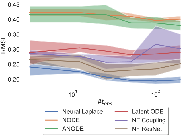
Figure 10: Test RMSE for Stiff Van de Pol Oscillator DE dataset analyzed. Averaged over 5 runs. We vary the number of observed points #$t_{obs}$ for each trajectory. Training for 200 epochs per dataset.

Appendix I Additional Benchmark Results

For fair comparison of the ODE based benchmarks, we also ran NODE and ANODE with the flexible solver method of ’dopri5’. Table 15 shows the test RMSE results, we observe Neural Laplace remains competitive.

Table 15: Test RMSE for datasets analyzed. Best result is bolded. Averaged over $5$ runs.

	Lotka-Volterra	ODE piecewise
Method	DDE	forcing function
NODE	0.5880 $\pm$ 0.0398	0.1945 $\pm$ 0.0134
ANODE	0.5673 $\pm$ 0.0744	0.0769 $\pm$ 0.0039
Neural Laplace	0.0427 $\pm$ 0.0066	0.0037 $\pm$ 0.0004

We also observe the same pattern seen in Table 4, when we add noise to the sampled DE systems. Table 12 shows results for Gaussian noise added to all the sampled trajectories of $\mathcal{N}(0,0.01)$, and Figure 19 shows some sampled test trajectories on one of these (Lotka-Volterra DDE) noise corrupted datasets.

Appendix J Benchmark Wall Clock Times

We measured the time to train on one epoch of 1,000 trajectories for each benchmark tested, detailed in Table 14, averaged over training for a 1,000 epochs. For completeness we include ’euler’ and ’dopri5’ solvers for NODE and ANODE methods. We observe that Neural Laplace is at least one order magnitude faster compared to ODE based solver methods, and in some cases up two orders of magnitude faster. We trained and took these readings on a Intel Xeon CPU @ 2.30GHz, 64GB RAM with a Nvidia Tesla V100 GPU 16GB.

Appendix K Training Loss Plots

Training loss plots against epochs can be seen in Figure 11. Empirically we see Neural Laplace can converge faster than the other benchmark methods.

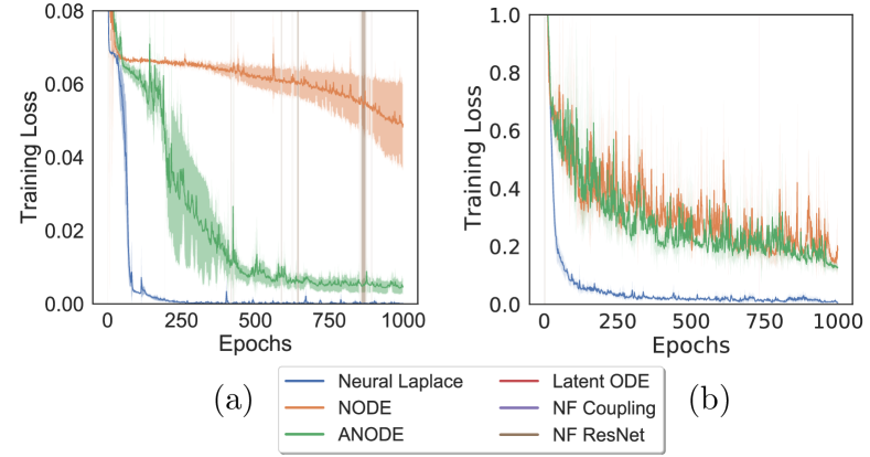
Figure 11: Training loss versus epochs, averaged over 5 runs, with standard deviation bars, training on the (a) ODE with piecewise forcing function dataset, (b) Lotka-Volterra DDE dataset.

Appendix L Extrapolating Toy Waveforms

We also explore the benchmarks and Neural Laplace at extrapolating toy waveform signals, that of a sawtooth, square and sine waveform. These are interesting to extrapolate as they are periodic and some contain discontinuities (square and sawtooth). We sampled each from the interval of $t\in[0,20]$, with a period of $2\pi$ for each waveform. We sampled different initial values by sampling a translation from $[0,2\pi]$ to generate different trajectories. These are given as sawtooth $x(t)=\frac{t}{2\pi}-\text{floor}(\frac{t}{2\pi})$, square $x(t)=2(1-\text{floor}\left(\frac{t}{\pi}\right)\%2)$ and sine $x(t)=\sin(t)$. The results of the methods in extrapolating these waveforms can be seen in Table L, with illustrations in Figures 16, 17, 18.

Appendix M Dataset Plots

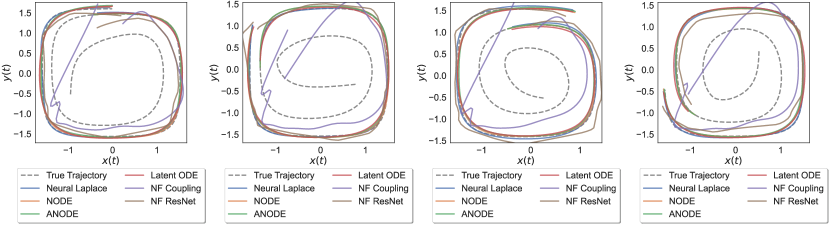
Figure 12: Spiral DDE randomly sampled test state plots.

Figure 13: Lotka-Volterra DDE randomly sampled test state plots.

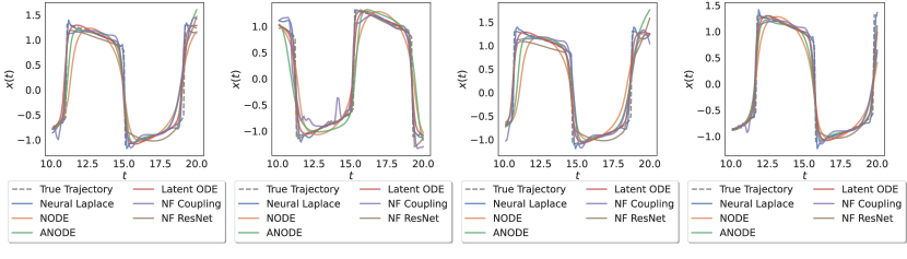
Figure 14: Stiff Van der Pol Oscillator DE randomly sampled test trajectory plots.

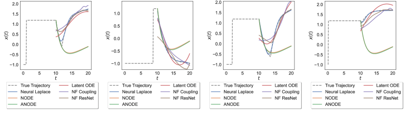
Figure 15: Mackey–Glass DDE modified to exhibit long range dependencies randomly sampled test trajectory plots.

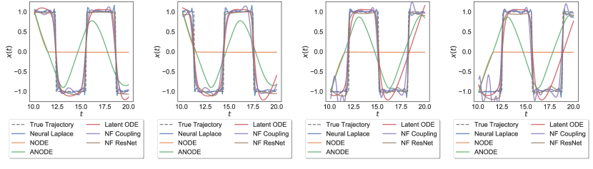
Figure 16: Square waveform randomly sampled test trajectory plots.

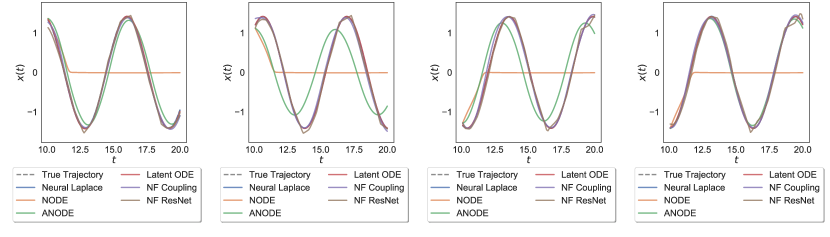
Figure 17: Sine waveform randomly sampled test trajectory plots.

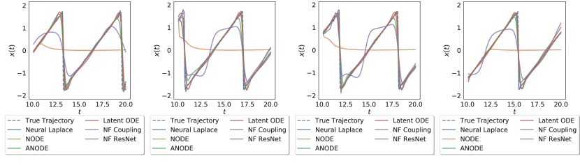
Figure 18: Sawtooth waveform randomly sampled test trajectory plots.

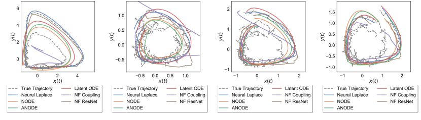
Figure 19: Lotka-Volterra DDE randomly sampled test state plots, with Gaussian noise added all trajectories of $\mathcal{N}(0,\epsilon)$, with $\epsilon=0.1$.

References

- Abate & Valko (2004) Abate, J. and Valko, P. P. Multi‐precision laplace transform inversion. International Journal for Numerical Methods in Engineering, 60:979–993, 2004.
- Al-Shuaibi (2001) Al-Shuaibi, A. Inversion of the laplace transform via post—widder formula. Integral Transforms and Special Functions, 11(3):225–232, 2001.
- Anumasa & PK (2021) Anumasa, S. and PK, S. Delay differential neural networks. In 2021 6th International Conference on Machine Learning Technologies, pp. 117–121, 2021.
- Åström & Murray (2010) Åström, K. J. and Murray, R. M. Feedback systems. Princeton university press, 2010.
- Bahar & Mao (2004) Bahar, A. and Mao, X. Stochastic delay lotka–volterra model. Journal of Mathematical Analysis and Applications, 292(2):364–380, 2004.
- Baker & Patil (1998) Baker, M. R. and Patil, R. B. Universal approximation theorem for interval neural networks. Reliable Computing, 4(3):235–239, 1998.
- Biloš et al. (2021) Biloš, M., Sommer, J., Rangapuram, S. S., Januschowski, T., and Günnemann, S. Neural flows: Efficient alternative to neural odes. Advances in Neural Information Processing Systems, 34, 2021.
- Bourne (2018) Bourne. Integro-Differential Equations. https://tinyurl.com/bourneintegrode, 2018. [Online; accessed 16-January-2022].
- Boyce et al. (2021) Boyce, W. E., DiPrima, R. C., and Meade, D. B. Elementary differential equations and boundary value problems. John Wiley & Sons, 2021.
- Chen et al. (2018) Chen, R. T., Rubanova, Y., Bettencourt, J., and Duvenaud, D. Neural ordinary differential equations. arXiv preprint arXiv:1806.07366, 2018.
- Cho et al. (2014) Cho, K., Van Merriënboer, B., Bahdanau, D., and Bengio, Y. On the properties of neural machine translation: Encoder-decoder approaches. arXiv preprint arXiv:1409.1259, 2014.
- Cimen & Uncu (2020) Cimen, E. and Uncu, S. On the solution of the delay differential equation via laplace transform. Communications in Mathematics and Applications, 11(3):379–387, 2020.
- Cooke (1963) Cooke, K. L. Differential—difference equations. In International symposium on nonlinear differential equations and nonlinear mechanics, pp. 155–171. Elsevier, 1963.
- Crann (2005) Crann, D. The laplace transform boundary element method for diffusion-type problems. 2005.
- De Hoog et al. (1982) De Hoog, F. R., Knight, J., and Stokes, A. An improved method for numerical inversion of laplace transforms. SIAM Journal on Scientific and Statistical Computing, 3(3):357–366, 1982.
- Debnath & Bhatta (2014) Debnath, L. and Bhatta, D. Integral transforms and their applications. CRC press, 2014.
- Dubner & Abate (1968) Dubner, H. and Abate, J. Numerical inversion of laplace transforms by relating them to the finite fourier cosine transform. Journal of the ACM (JACM), 15(1):115–123, 1968.
- Dupont et al. (2019) Dupont, E., Doucet, A., and Teh, Y. W. Augmented neural odes. In Proceedings of the 33rd International Conference on Neural Information Processing Systems, pp. 3140–3150, 2019.
- Filippov (2013) Filippov, A. F. Differential equations with discontinuous righthand sides: control systems, volume 18. Springer Science & Business Media, 2013.
- Forde (2005) Forde, J. E. Delay differential equation models in mathematical biology. University of Michigan, 2005.
- Ghosh et al. (2020) Ghosh, A., Behl, H., Dupont, E., Torr, P., and Namboodiri, V. Steer: Simple temporal regularization for neural ode. Advances in Neural Information Processing Systems, 33, 2020.
- Glass et al. (2021) Glass, D. S., Jin, X., and Riedel-Kruse, I. H. Nonlinear delay differential equations and their application to modeling biological network motifs. Nature communications, 12(1):1–19, 2021.
- Gwak et al. (2020) Gwak, D., Sim, G., Poli, M., Massaroli, S., Choo, J., and Choi, E. Neural ordinary differential equations for intervention modeling. arXiv preprint arXiv:2010.08304, 2020.
- Horváth et al. (2020) Horváth, G., Horváth, I., Almousa, S. A.-D., and Telek, M. Numerical inverse laplace transformation using concentrated matrix exponential distributions. Performance Evaluation, 137:102067, 2020.
- Jia & Benson (2019) Jia, J. and Benson, A. R. Neural jump stochastic differential equations. Advances in Neural Information Processing Systems, 32:9847–9858, 2019.
- Kexue & Jigen (2011) Kexue, L. and Jigen, P. Laplace transform and fractional differential equations. Applied Mathematics Letters, 24(12):2019–2023, 2011.
- Kidger et al. (2020a) Kidger, P., Chen, R. T., and Lyons, T. ” hey, that’s not an ode”: Faster ode adjoints with 12 lines of code. arXiv preprint arXiv:2009.09457, 2020a.
- Kidger et al. (2020b) Kidger, P., Morrill, J., Foster, J., and Lyons, T. Neural controlled differential equations for irregular time series. In Conference on Neural Information Processing Systems. Neural Information Processing Systems Foundation, 2020b.
- Kim et al. (2021) Kim, S., Ji, W., Deng, S., Ma, Y., and Rackauckas, C. Stiff neural ordinary differential equations. Chaos: An Interdisciplinary Journal of Nonlinear Science, 31(9):093122, 2021.
- Kingma & Ba (2017) Kingma, D. P. and Ba, J. Adam: A method for stochastic optimization, 2017.
- Koch et al. (2014) Koch, G., Krzyzanski, W., Pérez-Ruixo, J. J., and Schropp, J. Modeling of delays in pkpd: classical approaches and a tutorial for delay differential equations. Journal of Pharmacokinetics and Pharmacodynamics, 41:291–318, 2014.
- Kuhlman (2013) Kuhlman, K. L. Review of inverse laplace transform algorithms for laplace-space numerical approaches. Numerical Algorithms, 63(2):339–355, 2013.
- Lindeberg (2022) Lindeberg, T. A time-causal and time-recursive scale-covariant scale-space representation of temporal signals and past time. arXiv preprint arXiv:2202.09209, 2022.
- Lindeberg & Fagerström (1996) Lindeberg, T. and Fagerström, D. Scale-space with casual time direction. In European conference on computer vision, pp. 229–240. Springer, 1996.
- López (2020) López, A. G. On an electrodynamic origin of quantum fluctuations. Nonlinear Dynamics, 102(1):621–634, 2020.
- Mackey & Glass (1977) Mackey, M. C. and Glass, L. Oscillation and chaos in physiological control systems. Science, 197(4300):287–289, 1977.
- Medlock (2004) Medlock, J. P. Integro-differential-equation models in ecology and epidemiology. University of Washington, 2004.
- Moreira Gomes et al. (2019) Moreira Gomes, J., Lobosco, M., Weber dos Santos, R., and Cherry, E. M. Delay differential equation-based models of cardiac tissue: Efficient implementation and effects on spiral-wave dynamics. Chaos: An Interdisciplinary Journal of Nonlinear Science, 29(12):123128, 2019.
- Moridis (1992) Moridis, G. Alternative formulations of the laplace transform boundary element (ltbe) numerical method for the solution of diffusion-type equations. In Boundary element technology VII, pp. 815–833. Springer, 1992.
- Moridis & Reddel (1991) Moridis, G. and Reddel, D. The laplace transform boundary element (ltbe) method for the solution of diffusion-type equations. In Boundary elements XIII, pp. 83–97. Springer, 1991.
- Moridis et al. (1994) Moridis, G., McVay, D., Reddell, D., and Blasingame, T. The laplace transform finite difference (ltfd) numerical method for the simulation of compressible liquid flow in reservoirs. SPE Advanced Technology Series, 2(02):122–131, 1994.
- Moridis & Reddell (1991) Moridis, G. J. and Reddell, D. L. The laplace transform finite difference method for simulation of flow through porous media. Water Resources Research, 27(8):1873–1884, 1991.
- Paszke et al. (2017) Paszke, A., Gross, S., Chintala, S., Chanan, G., Yang, E., DeVito, Z., Lin, Z., Desmaison, A., Antiga, L., and Lerer, A. Automatic differentiation in pytorch. In NIPS-W, 2017.
- Podlubny (1997) Podlubny, I. The laplace transform method for linear differential equations of the fractional order. arXiv preprint funct-an/9710005, 1997.
- Pospisil & Jaros (2016) Pospisil, M. and Jaros, F. On the representation of solutions of delayed differential equations via laplace transform. Electronic Journal of Qualitative Theory of Differential Equations, 2016(117):1–13, 2016.
- Poularikas (2018) Poularikas, A. D. Transforms and applications handbook. CRC press, 2018.
- Rubanova et al. (2019) Rubanova, Y., Chen, R. T. Q., and Duvenaud, D. Latent odes for irregularly-sampled time series. CoRR, abs/1907.03907, 2019.
- Rudin (1987) Rudin, W. Real and Complex Analysis, 3rd Ed. McGraw-Hill, Inc., USA, 1987. ISBN 0070542341.
- Sachs & Strauss (2008) Sachs, E. and Strauss, A. Efficient solution of a partial integro-differential equation in finance. Applied Numerical Mathematics, 58(11):1687–1703, 2008.
- Sandu et al. (1997) Sandu, A., Verwer, J., Van Loon, M., Carmichael, G., Potra, F., Dabdub, D., and Seinfeld, J. Benchmarking stiff ode solvers for atmospheric chemistry problems-i. implicit vs explicit. Atmospheric environment, 31(19):3151–3166, 1997.
- Schiff (1999) Schiff, J. L. The Laplace transform: theory and applications. Springer Science & Business Media, 1999.
- Schmidt et al. (2020) Schmidt, D., Koppe, G., Monfared, Z., Beutelspacher, M., and Durstewitz, D. Identifying nonlinear dynamical systems with multiple time scales and long-range dependencies. In International Conference on Learning Representations, 2020.
- Shampine & Reichelt (1997) Shampine, L. F. and Reichelt, M. W. The matlab ode suite. SIAM journal on scientific computing, 18(1):1–22, 1997.
- Smith (1997) Smith, S. W. The Scientist and Engineer’s Guide to Digital Signal Processing. California Technical Publishing, USA, 1997. ISBN 0966017633.
- Stehfest (1970) Stehfest, H. Algorithm 368: Numerical inversion of laplace transforms [d5]. Communications of the ACM, 13(1):47–49, 1970.
- Su et al. (2021) Su, W.-H., Chou, C.-S., and Xiu, D. Deep learning of biological models from data: Applications to ode models. Bulletin of Mathematical Biology, 83(3):1–19, 2021.
- Talbot (1979) Talbot, A. The accurate numerical inversion of laplace transforms. IMA Journal of Applied Mathematics, 23(1):97–120, 1979.
- Teschl (2012) Teschl, G. Ordinary differential equations and dynamical systems, volume 140. American Mathematical Soc., 2012.
- Van der Pol & Van Der Mark (1927) Van der Pol, B. and Van Der Mark, J. Frequency demultiplication. Nature, 120(3019):363–364, 1927.
- Ver Steeg (2000) Ver Steeg, G. Non-parametric entropy estimation toolbox (npeet). Technical report, Technical Report. 2000. Available online: https://www. isi. edu/~ gregv …, 2000.
- Verdugo & Rand (2007) Verdugo, A. and Rand, R. H. Delay differential equations in the dynamics of gene copying. In International Design Engineering Technical Conferences and Computers and Information in Engineering Conference, volume 4806, pp. 681–686, 2007.
- Yi et al. (2006) Yi, S., Ulsoy, A. G., and Nelson, P. W. Solution of systems of linear delay differential equations via laplace transformation. In Proceedings of the 45th IEEE Conference on Decision and Control, pp. 2535–2540. IEEE, 2006.
- Yildiz et al. (2019) Yildiz, C., Heinonen, M., and Lähdesmäki, H. Ode2vae: Deep generative second order odes with bayesian neural networks. In Conference on Neural Information Processing Systems. Neural Information Processing Systems Foundation, 2019.
- Yousef & Ismail (2018) Yousef, H. M. and Ismail, A. M. Application of the laplace adomian decomposition method for solution system of delay differential equations with initial value problem. In AIP Conference Proceedings, volume 1974, pp. 020038. AIP Publishing LLC, 2018.
- Zahra et al. (2017) Zahra, W., Hikal, M., and Bahnasy, T. A. Solutions of fractional order electrical circuits via laplace transform and nonstandard finite difference method. Journal of the Egyptian Mathematical Society, 25(2):252–261, 2017.
- Zhu et al. (2020) Zhu, Q., Guo, Y., and Lin, W. Neural delay differential equations. In International Conference on Learning Representations, 2020.
- Zill (2016) Zill, D. G. Differential equations with boundary-value problems. Cengage Learning, 2016.
- Zulko (2019) Zulko. Delay Differential Equation Solver. https://github.com/Zulko/ddeint, 2019. [Online; accessed 26-January-2022].