A Novel Partitioned Approach for Reduced Order Model - Finite Element Model (ROM-FEM) and ROM-ROM Coupling

ABSTRACT

Partitioned methods allow one to build a simulation capability for coupled problems by reusing existing single-component codes. In so doing, partitioned methods can shorten code development and validation times for multiphysics and multiscale applications. In this work, we consider a scenario in which one or more of the “codes” being coupled are projection-based reduced order models (ROMs), introduced to lower the computational cost associated with a particular component. We simulate this scenario by considering a model interface problem that is discretized independently on two non-overlapping subdomains. We then formulate a partitioned scheme for this problem that allows the coupling between a ROM “code” for one of the subdomains with a finite element model (FEM) or ROM “code” for the other subdomain. The ROM “codes” are constructed by performing proper orthogonal decomposition (POD) on a snapshot ensemble to obtain a low-dimensional reduced order basis, followed by a Galerkin projection onto this basis. The ROM and/or FEM “codes” on each subdomain are then coupled using a Lagrange multiplier representing the interface flux. To partition the resulting monolithic problem, we first eliminate the flux through a dual Schur complement. Application of an explicit time integration scheme to the transformed monolithic problem decouples the subdomain equations, allowing their independent solution for the next time step. We show numerical results that demonstrate the proposed method’s efficacy in achieving both ROM-FEM and ROM-ROM coupling.

INTRODUCTION

Partitioned schemes enable the rapid development of simulation capabilities for coupled problems from existing codes for the individual sub-models; see, e.g., (maxnames[12], deBoer_07_CMAME) for examples. Besides being a cost-effective alternative to the development of monolithic multiphysics codes from scratch, a partitioned approach can also improve simulation efficiency by employing codes tailored to the salient physics characteristics of the sub-models.

Typically, the sub-model codes in partitioned schemes implement high-fidelity full-order models (FOMs) based on conventional discretizations such as finite elements, finite volumes or finite differences. However, it is not uncommon to encounter situations in which one or more of these full order models become performance bottlenecks. For example, in blast-on-structure simulations (maxnames[6], Bessette_03a_INPROC), calculation of the wave propagation by a high-fidelity scheme can be computationally expensive and is often replaced with direct structure loading by means of simplified boundary conditions derived using analytic techniques (maxnames[31], Randers-Pehrson_97_ARL). However, such conditions assume simple geometries and cannot account for wave interactions with more complex fluid-structure interfaces. A better alternative in this context would be a hybrid partitioned scheme in which the expensive full-order sub-model is replaced by a computationally efficient, yet physically faithful, reduced order model (ROM).

To demonstrate the potential of a coupling approach of the type described above, we formulate herein a new hybrid explicit partitioned scheme that enables the coupling of conventional finite element models (FEM) with projection-based ROMs (more specifically, ROMs constructed using the Proper Orthogonal Decomposition (POD)/Galerkin projection method (maxnames[3], Holmes:1988; maxnames[18], Holmes:1996; maxnames[32], Sirovich:1987). We describe and develop our methodology in the context of a generic advection-diffusion transmission problem posed on a decomposition of the physical domain into two non-overlapping subdomains. Although simple and comprised of a single physics, this problem configuration is sufficient to simulate a typical setting for the development of a partitioned scheme.

Our scheme extends the approach in (maxnames[28], AdC:CAMWA), which starts from a monolithic formulation of the transmission problem, uses a Schur complement to obtain an approximation of the interface flux, and then inserts this flux as a Neumann boundary condition into each subdomain problem. Application of an explicit time integration scheme to this transformed monolithic problem decouples its subdomain problems and allows their independent solution.

In addition to enabling a hybrid partitioned analysis for coupled problems, our approach can also be used to perform a hybrid reduced order model - full order model (ROM-FOM) analysis (maxnames[24], Lucia:2001; maxnames[25], Lucia:2003; maxnames[22], LeGresley:2003; maxnames[21], LeGresley:2005; maxnames[8], Buffoni:2007; maxnames[4], Baiges:2013; maxnames[10], Corigliano:2015). In this approach, the physical domain of a given, usually single physics, partial differential equation (PDE) problem is decomposed into two or more subdomains, and either a ROM or a FOM is constructed in each subdomain based on the solution characteristics. The resulting models are then coupled in some way to obtain a global solution on the physical domain in its entirety. Such an analysis can mitigate robustness and accuracy issues of projection-based model order reduction, especially when applied to highly non-linear and/or convection-dominated problems.

In contrast to traditional partitioned schemes (maxnames[15], Gatzhammer_14_THESIS; maxnames[29], Piperno_01_CMAME; maxnames[5], Banks_17_JCP) and methods for hybrid ROM-FOM analyses (maxnames[22], LeGresley:2003; maxnames[21], LeGresley:2005; maxnames[8], Buffoni:2007; maxnames[9], Cinquegrana:2011; maxnames[27], Maier:2014), our framework is monolithic rather than iterative, enabling one to obtain the coupled ROM-ROM or ROM-FEM solution in a single shot. Also, unlike the work in (maxnames[1], Ammar:2011; maxnames[19], Iapichino:2016; maxnames[13], Eftang:2013; maxnames[14], Eftang:2014; maxnames[17], Hoang:2021), there is no need in our formulation to construct boundary, port, or skeleton bases for enforcing inter-subdomain compatibility. Furthermore, while our formulation shares some commonalities with existing Lagrange multiplier-based coupling methods such as those of (maxnames[24], Lucia:2001; maxnames[25], Lucia:2003; maxnames[26], Maday:2004; maxnames[2], Antil:2010; maxnames[11], Corigliano:2013; maxnames[10], Corigliano:2015; maxnames[20], Kerfriden:2013; maxnames[30], Radermacher:2014; maxnames[4], Baiges:2013), we emphasize that our approach is fundamentally different from these methods in that it enables the complete decoupling of the underlying models (ROMs and/or FOMs) at each time-step of the time-integration scheme used to advance the discretized PDE forward in time. Importantly, our methodology delivers a smooth and accurate solution without the need to introduce ad hoc correction/stabilization terms, such as those proposed in (maxnames[22], LeGresley:2003; maxnames[21], LeGresley:2005; maxnames[4], Baiges:2013).

The remainder of this paper is organized as follows. In Section 2, we introduce our model transmission problem, derive the relevant monolithic formulation and discretize it in space. Section 3 explains the elimination of the Lagrange multiplier through a dual Schur complement, which transforms the semi-discrete system into another coupled problem that serves as a basis for the development of our partitioned scheme. In Section 4, we describe our POD/Galerkin ROM construction methodology, and detail the application of the approach described in Section 3 to ROM-FEM and ROM-ROM coupling. We evaluate the performance of the proposed scheme on a two-dimensional (2D) model problem in Section 5. Finally, conclusions are offered in Section 6.

A MODEL TRANSMISSION PROBLEM

We consider a bounded region $\Omega\subset\mathbb{R}^{d}$, $d=2,3$ with a Lipschitz-continuous boundary $\Gamma$. We assume that $\Omega$ is divided into two non-overlapping subdomains $\Omega_{1}$ and $\Omega_{2}$, each with boundary $\partial\Omega_{i}$ for $i=1,2$. Let $\gamma$ denote the interface shared between the two subdomains, and let $\Gamma_{i}=\partial\Omega_{i}\backslash\gamma$ for $i=1,2$, as illustrated in Figure 1.

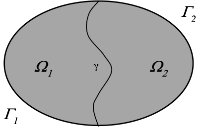
Figure 1: Non-overlapping subdomains

We take $\mathbf{n}_{\gamma}$ to be the unit normal on the interface pointing toward $\Omega_{2}$. We use a setting comprising two non-overlapping domains to avoid technical complications that are not germane to the core topic of the paper. Our approach can be extended to configurations involving multiple domains as long as one incorporates a proper mechanism to handle floating subdomains, such as the techniques in (maxnames[7], Bochev_05_SIREV).

We consider a model transmission problem given by the advection-diffusion equation:

$$\begin{split}\dot{\varphi_{i}}-\nabla\cdot F_{i}(\varphi_{i})&=f_{i}\hskip 14.22636pt\text{ on }\Omega_{i}\times[0,T]\\ \varphi_{i}&=g_{i}\hskip 14.22636pt\text{ on }\Gamma_{i}\times[0,T],\hskip 5.69054pti=1,2,\end{split}$$ (1)

where the over-dot notation denotes differentiation in time, the unknown $\varphi_{i}$ is a scalar field, $F_{i}(\varphi_{i})=\kappa_{i}\nabla\varphi_{i}-\mathbf{u}\varphi_{i}$ is the total flux function, $\kappa_{i}>0$ is the diffusion coefficient in $\Omega_{i}$, and $\mathbf{u}$ the velocity field. We augment (1) with initial conditions:

$$\varphi_{i}(\mathbf{x},0)=\varphi_{i,0}(\mathbf{x})\hskip 14.22636pt\text{ in }\Omega_{i},\hskip 5.69054pti=1,2\,.$$ (2)

Along the interface $\gamma$, we enforce continuity of the states and continuity of the total flux, giving rise to the following interface conditions:

$$\varphi_{1}(\mathbf{x},t)-\varphi_{2}(\mathbf{x},t)=0\hskip 5.69054pt\text{ and }F_{1}(\mathbf{x},t)\cdot\mathbf{n}_{\gamma}=F_{2}(\mathbf{x},t)\cdot\mathbf{n}_{\gamma}\hskip 5.69054pt\text{ on }\gamma\times[0,T].$$ (3)

We note that one also has the option to enforce only equilibrium of the diffusive flux exchanged between the two subdomains. We do not consider this option here, as the resulting partitioned scheme will be similar to the one obtained by enforcing continuity of the total flux.

In contrast to conventional, loosely coupled partitioned schemes (see, e.g., (maxnames[12], deBoer_07_CMAME)), our approach starts from a well-posed monolithic formulation of (1)–(3). To obtain this formulation let $V:=H^{1}_{\Gamma}(\Omega_{1})\times H^{1}_{\Gamma}(\Omega_{2})\times H^{-1/2}(\gamma)$. Using a Lagrange multiplier to enforce continuity of states, i.e., the first condition in (3), yields the following monolithic weak problem: find $\{\varphi_{1},\varphi_{2},\lambda\}\in C^{1}([0,T];V)$, such that for all $t\in(0,T]$

$$\begin{split}(\dot{\varphi_{1}},\nu)_{\Omega_{1}}+(\kappa_{1}\nabla\varphi_{1},\nabla\nu)_{\Omega_{1}}-(\mathbf{u}\varphi_{1},\nabla\nu)_{\Omega_{1}}+(\lambda,\nu)_{\gamma}&=(f_{1},\nu)_{\Omega_{1}}\hskip 14.22636pt\forall\nu\in H^{1}_{\Gamma}(\Omega_{1})\\ (\dot{\varphi_{2}},\eta)_{\Omega_{2}}+(\kappa_{2}\nabla\varphi_{2},\nabla\eta)_{\Omega_{2}}-(\mathbf{u}\varphi_{2},\nabla\eta)_{\Omega_{2}}-(\lambda,\eta)_{\gamma}&=(f_{2},\eta)_{\Omega_{2}}\hskip 14.22636pt\forall\eta\in H^{1}_{\Gamma}(\Omega_{2})\\ (\varphi_{1},\mu)_{\gamma}-(\varphi_{2},\mu)_{\gamma}&=0\hskip 48.36967pt\forall\mu\in H^{-1/2}(\gamma).\end{split}$$ (4)

It is easy to see that the Lagrange multiplier $\lambda$ is the flux exchanged through the interface, i.e., $\lambda=F_{1}\cdot\mathbf{n}_{\gamma}=F_{2}\cdot\mathbf{n}_{\gamma}$. This observation is at the core of our partitioned method formulation. Indeed, if we could somehow determine $\lambda$, then each subdomain problem becomes a well-posed mixed boundary value problem with a Neumann condition on $\gamma$ provided by $\lambda$:

$$\begin{split}\dot{\varphi_{i}}-\nabla\cdot F_{i}(\varphi_{i})&=f_{i}\hskip 42.67912pt\text{ on }\Omega_{i}\times[0,T]\\ \varphi_{i}&=g_{i}\hskip 42.67912pt\text{ on }\Gamma_{i}\times[0,T]\\ F_{i}(\varphi_{i})\cdot\mathbf{n}_{i}&=(-1)^{i}\lambda\hskip 22.76219pt\text{ on }\gamma\times[0,T]\end{split}\,,\quad i=1,2\,.$$ (5)

In other words, knowing $\lambda$ could allow us to decouple the subdomain equations and solve them independently. Of course, this cannot be done within the framework of (4), which is a fully coupled problem in terms of the states $\phi_{i}$ and the Lagrange multiplier $\lambda$. However, an independent estimation of $\lambda$ may be possible in the context of a discretized version of this coupled problem.

A SEMI-DISCRETE MONOLITHIC FORMULATION

Let $V^{h}\subset V$ be a conforming finite element space spanned by a basis $\{\nu_{i},\eta_{j},\mu_{k}\}$; $i=1,\ldots,N_{1}$; $j=1,\ldots,N_{2}$; $k=1,\ldots,N_{\gamma}$. A finite element discretization of (4) yields the following system of Differential Algebraic Equations (DAEs):

$$\begin{split}M_{1}\dot{\bm{\Phi}}_{1}+G_{1}^{T}\bm{\lambda}&=\mathbf{\overline{f}}_{1}(\bm{\Phi}_{1})\\ M_{2}\dot{\bm{\Phi}}_{2}-G_{2}^{T}\bm{\lambda}&=\mathbf{\overline{f}}_{2}(\bm{\Phi}_{2})\\ G_{1}\bm{\Phi}_{1}-G_{2}\bm{{\Phi}}_{2}&=\bm{0},\end{split}$$ (6)

where for $r=1,2$, $\bm{\Phi}_{r}$ are the coefficient vectors corresponding to $\varphi_{r}$, $M_{r}$ are the mass matrices, the right hand side vector $\mathbf{\overline{f}}_{r}(\bm{\Phi}_{r}):=\mathbf{f}_{r}-(D_{r}+A_{r})\bm{\Phi}_{r}$ with $D_{r},A_{r}$ corresponding to the diffusive and advective flux terms, respectively, and $G_{r}$ are the matrices enforcing the (weak) continuity of the states. Assembly of these matrices is standard, for example, $(M_{1})_{ij}=(\nu_{j},\nu_{i})_{\Omega_{1}}$, $(D_{2})_{ij}=\kappa_{2}(\nabla\eta_{j},\nabla\eta_{i})_{\Omega_{2}}$; $(G_{1})_{i,j}=(\nu_{j},\mu_{i})_{\gamma}$; $(G_{2})_{i,j}=(\eta_{j},\mu_{i})_{\gamma}$, and so on. We note here that the space for the Lagrange multiplier $\lambda$ can be taken to be the trace of the finite element space on either of $\Omega_{1}$ or $\Omega_{2}$; either choice will be stable. In practice, using the coarser of the two interface spaces for the Lagrange multiplier space improves accuracy; see (maxnames[28], AdC:CAMWA) and (maxnames[33], AdC:RINAM) for details and discussion.

EXPLICIT PARTITIONED SCHEME FOR FEM-FEM COUPLING

In this section, we briefly review the Implicit Value Recovery (IVR) scheme (maxnames[28], AdC:CAMWA), which provides the basis for our new hybrid partitioned approach. Then, in Section 4, we discuss extensions of IVR to include a ROM in one or both subdomains.

The IVR scheme (maxnames[28], AdC:CAMWA) is predicated on the ability to express $\bm{\lambda}$ as an implicit function of the subdomain states. This, however, is not possible for (6) because it is an Index-2 Hessenberg DAE. In (maxnames[28], AdC:CAMWA), we resolved this issue by differentiating the constraint equation in time. This step reduced the index of (6) and produced the following Index-1 Hessenberg DAE:

$$\begin{split}M_{1}\dot{\bm{\Phi}}_{1}+G_{1}^{T}\bm{\lambda}&=\mathbf{\overline{f}}_{1}(\bm{\Phi}_{1})\\ M_{2}\dot{\bm{\Phi}}_{2}-G_{2}^{T}\bm{\lambda}&=\mathbf{\overline{f}}_{2}(\bm{\Phi}_{2})\\ G_{1}\dot{\bm{\Phi}}_{1}-G_{2}\dot{\bm{{\Phi}}}_{2}&=0\;\;.\end{split}$$ (7)

Assuming the initial data are continuous across $\gamma$, the new constraint $(\dot{\varphi_{1}},\mu)_{\gamma}-(\dot{\varphi_{2}},\mu)_{\gamma}=0$ is equivalent to the original one, i.e., (7) is equivalent to the original monolithic problem (6). In what follows we refer to (7) as the FEM-FEM model. This model can be written in matrix form as:

$$\begin{bmatrix}M_{1}&0&G_{1}^{T}\\ 0&M_{2}&-G_{2}^{T}\\ G_{1}&-G_{2}&0\end{bmatrix}\begin{bmatrix}\dot{\bm{\Phi}}_{1}\\ \dot{\bm{\Phi}}_{2}\\ \bm{\lambda}\end{bmatrix}=\begin{bmatrix}\mathbf{\overline{f}}_{1}(\bm{\Phi}_{1})\\ \mathbf{\overline{f}}_{2}(\bm{\Phi}_{2})\\ 0\end{bmatrix}\,.$$ (8)

To explain IVR it is further convenient to write (8) in the canonical semi-explicit DAE form:

$$\begin{split}\dot{y}&=f(t,y,z)\\ 0&=g(t,y,z)\end{split}$$ (9)

where $y=(\bm{\Phi}_{1},\bm{\Phi}_{2})$ is the differential variable, $z=\bm{\lambda}$ is the algebraic variable,

$$\begin{split}f(t,y,z)&=\begin{pmatrix}M_{1}^{-1}\Big{(}\overline{\mathbf{f}}_{1}(\bm{\Phi}_{1})-G_{1}^{T}\bm{\lambda}\Big{)}\\ M_{2}^{-1}\Big{(}(\overline{\mathbf{f}}_{2}(\bm{\Phi}_{2})+G_{2}^{T}\bm{\lambda}\Big{)}\end{pmatrix}\end{split}\;,$$ (10)

and

$$g(t,y,z)=S\bm{\lambda}-G_{1}M_{1}^{-1}\overline{\mathbf{f}}_{1}(\bm{\Phi}_{1})+G_{2}M_{2}^{-1}\overline{\mathbf{f}}_{2}(\bm{\Phi}_{2})\,.$$ (11)

The matrix $S:=G_{1}M_{1}^{-1}G_{1}^{T}+G_{2}M_{2}^{-1}G_{2}^{T}$ in (11) is the Schur complement of the upper left $2\times 2$ block submatrix of the matrix in (8). It can be shown that the Schur complement $S$ is nonsingular; see Proposition 4.1 in (maxnames[28], AdC:CAMWA). This implies that the Jacobian $\partial_{z}g=S$ is also nonsingular for all $t$. As a result, the equation $g(t,y,z)=0$ defines $z$ as an implicit function of the differential variable. After solving this equation for the algebraic variable and inserting the solution $\bm{\lambda}(\bm{\Phi}_{1},\bm{\Phi}_{2})$ into (8) we obtain a coupled system of ODEs in terms of the states:

$$\begin{bmatrix}M_{1}&0\\ 0&M_{2}\end{bmatrix}\begin{bmatrix}\dot{\bm{\Phi}}_{1}\\ \dot{\bm{\Phi}}_{2}\end{bmatrix}=\begin{bmatrix}\mathbf{\overline{f}}_{1}(\bm{\Phi}_{1})-G_{1}^{T}\bm{\lambda}(\bm{\Phi}_{1},\bm{\Phi}_{2})\\ \mathbf{\overline{f}}_{2}(\bm{\Phi}_{2})+G_{2}^{T}\bm{\lambda}(\bm{\Phi}_{1},\bm{\Phi}_{2})\end{bmatrix}\;.$$ (12)

The IVR scheme is based on the observation that application of an explicit time integration scheme to discretize (12) in time effectively decouples the equations and makes it possible to solve them independently.

The IVR algorithm for solving the coupled system is now as follows. Let $D^{n}_{t}(\bm{\Phi})$ be a forward time differencing operator such as the Forward Euler operator $D^{n}_{t}(\bm{\Phi})=(\bm{\Phi}^{n+1}-\bm{\Phi}^{n})/\Delta t$. For each time step $t^{n}$:

1. Compute modified forces: for $i=1,2$ use $\bm{\Phi}_{i}^{n}$ to compute the vector

   $$\widetilde{\bm{f}}_{i}^{n}:=\overline{\mathbf{f}}_{i}(\bm{\Phi}_{i}^{n})=\mathbf{f}_{i}-(D_{i}+A_{i})\bm{\Phi}_{i}^{n}.$$

2. Compute the Lagrange multiplier: solve the Schur complement system

   $$\Big{(}G_{1}M_{1}^{-1}G_{1}^{T}+G_{2}M_{2}^{-1}G_{2}^{T}\Big{)}\bm{\lambda}^{n}=G_{1}M_{1}^{-1}\widetilde{\bm{f}}_{1}^{n}-G_{2}M_{2}^{-1}\widetilde{\bm{f}_{2}^{n}}$$

   for $\bm{\lambda}^{n}$. Compute $G_{1}^{T}\bm{\lambda}^{n}$ and $G_{2}^{T}\bm{\lambda}^{n}$.

3. Update the state variables: for $i=1,2$, solve the systems

   $$M_{i}D^{n}_{t}(\bm{\Phi}_{i})=\widetilde{\bm{f}}_{i}^{n}+(-1^{i})G_{i}^{T}\bm{\lambda}^{n}.$$

DEVELOPMENT OF HYBRID PARTITIONED SCHEMES

In this section, we present the extension of the IVR method, described in Section 3, to a hybrid partitioned scheme, which couples ROM to FEM or to another ROM. Specifically, in Section 4.2, we present the details for the case where a projection-based ROM is employed in one of the two subdomains shown in Figure 1; then, in Section 4.3, we briefly describe the ROM-ROM extension of our coupling methodology.

To define the ROM component within our coupling, we use a proper orthogonal decomposition (POD) approach. A typical POD-based model order reduction is comprised of two distinct stages. In the first stage, one uses samples obtained by solving a suitable FOM to construct a reduced basis, usually by computing a truncated singular value decomposition (SVD) of the sample set. We discuss this stage in Section 4.1. At the second stage, one replaces the conventional finite element test and trial functions in a weak formulation of the governing equations by reduced basis functions. This stage projects the weak problem onto the reduced basis and is discussed in Section 4.2.

Obtaining a quality ROM that is both computationally efficient and accurate in the predictive regime is a non-trivial endeavor on its own. Since our main goal is the development of the hybrid partitioned approach rather than the ROM, in this work we will follow standard, established procedures to obtain the necessary ROMs.

REDUCED BASIS CONSTRUCTION

Without loss of generality, we shall describe the first stage of the POD-based model order reduction for $\Omega_{1}$. In this work, we have adopted a workflow in which the snapshots in $\Omega_{1}$ are collected by performing a global (uncoupled) FEM simulation in $\Omega$, restricting the resulting finite element solution to $\Omega_{1}$, and then sampling the restricted solution over $m$ uniform time steps. Let $\Delta_{s}t$ denote the sampling time step, $t_{k}=k(\Delta_{s}t)$, $k=1,\ldots m$, the sampling time points, and $\bm{\Phi}_{1}(t_{k})\in\mathbb{R}^{N_{1}}$ the $k$th snapshot, i.e., the coefficient vector of the restricted finite element solution at $t_{k}$.

We arrange the snapshots in an $N_{1}\times m$ matrix $X$ whose $k$th column is the $k$th snapshot $\bm{\Phi}_{1}(t_{k})$. The coefficients in each snapshot form two distinct groups. The first one contains the coefficients associated with the nodes on the Dirichlet boundary $\Gamma_{1}$. These coefficients contain the values of the boundary condition function $g_{1}$ at the these nodes, and so we call them Dirichlet coefficients. The coefficients in the second group correspond to the nodes in the interior of $\Omega_{1}$ and the nodes on the interface $\gamma$. We refer to these coefficients as the free coefficients, as they are the unknowns in the finite element discretization of the subdomain PDE (5) on $\Omega_{1}$.

Performing a POD-based model order reduction for problems with Dirichlet boundary conditions requires some care in the generation of the reduced basis and the subsequent imposition of the Dirichlet conditions on the ROM solution. Herein, we use an approach that represents an extension of a common finite element technique that imposes essential boundary conditions via a boundary interpolant of the data $g_{1}$; see (maxnames[16], Gunzburger:2007) for more details. Below we describe how this technique is applied to the generation of the reduced basis, and in Section 4.2, we explain the imposition of the boundary conditions within the ROM formulation.

Let $\bm{\beta}_{k}\in\mathbb{R}^{N_{1}}$ denote a vector whose free coefficients are all set to zero and whose Dirichlet coefficients are set to the nodal values of the boundary data at $t_{k}$, that is,

$$(\bm{\beta}_{k})_{i}=\left\{\begin{array}[]{rl}g_{1}(\mathbf{x}_{i},t_{k})&\mbox{if $\mathbf{x}_{i}\in\Gamma_{1}$}\\[4.30554pt] 0&\mbox{if $\mathbf{x}_{i}\in\Omega_{1}\cup\gamma$}\end{array}\;.\right.$$ (13)

Following (maxnames[16], Gunzburger:2007) we define the adjusted snapshot matrix $X_{0}$ by subtracting $\bm{\beta}_{k}$ from the $k$th column of $X$, i.e., we set the $k$th column of $X_{0}$ to $\bm{\Phi}_{1}(t_{k})-\bm{\beta}_{k}$.

Next, we compute the singular value decomposition of the adjusted matrix, $X_{0}=U_{0}\Sigma_{0}V^{T}_{0}$, and choose an integer $N_{R}\ll N_{1}$. The reduced basis is then defined as the first $N_{R}$ left singular vectors of the SVD decomposition, i.e., the first $N_{R}$ columns of $U_{0}$. We denote the matrix containing these columns by $\widetilde{U}_{0}$.

Each column of $\widetilde{U}_{0}$ can be mapped to a finite element function whose nodal coefficients are the entries in this column. These finite element functions can be construed as a new reduced order basis for the finite element space. Note that these basis functions are globally supported rather than locally supported, as is the case with traditional finite element basis functions. Thus, using the reduced basis functions as test and trial functions in a weak formulation of (5) results in dense algebraic problems. Consequently, an effective ROM requires $N_{R}$ to be as small as possible. A simple approach is to choose a tolerance level $\delta$ and remove the columns of $U_{0}$ corresponding to all singular values that are less than $\delta$. We note that $\delta$ should be such that no columns of $U_{0}$ are retained which correspond to singular values sufficiently close to 0. These columns of $U_{0}$ span a near null space, which we do not want to retain as part of the reduced basis.

IVR EXTENSION TO ROM-FEM COUPLING

To extend the IVR scheme in Section 3 from a FEM-FEM to a ROM-FEM coupling with a ROM on $\Omega_{1}$, we will perform the second model order reduction stage directly in the monolithic formulation of the model problem. Formally, this amounts to discretizing the first equation in (4) using the global basis functions (POD modes) corresponding to the columns of $\widetilde{U}_{0}$ instead of the standard finite element basis functions. In practice, for linear problems, the matrices defining the ROM can be be easily obtained from the already assembled full order model matrices. Thus, we will implement the second stage using the transformed semi-discrete monolithic problem, i.e., the Index-1 DAE (7).

For simplicity, in discussing this stage, we shall assume that the Dirichlet boundary condition function $g_{1}$ is independent of time. In this case, the vectors $\bm{\beta}_{k}$ defined in (13) are identical to a vector $\bm{\beta}$ whose free coefficients are zero and Dirichlet coefficients are the nodal values of $g_{1}$. To obtain the ROM on $\Omega_{1}$ we perform a state transformation of the first equation in (7) by inserting the ansatz $\bm{\Phi}_{1}=\widetilde{U}_{0}\bm{\varphi}_{R}+\bm{\beta}$ into that equation. Then, we multiply the first equation by $\widetilde{U}^{T}_{0}$ to obtain the following ROM-FEM monolithic problem:

$$\begin{split}\widetilde{M}_{1}\dot{\bm{\varphi}}_{R}+\widetilde{G}^{T}_{1}\bm{\lambda}&=\widetilde{U}^{T}_{0}\overline{\mathbf{f}}_{1}(\widetilde{U}_{0}\bm{\varphi}_{R}+\bm{\beta})\\ M_{2}\dot{\bm{\Phi}}_{2}-G_{2}^{T}\bm{\lambda}&=\overline{\mathbf{f}}_{2}(\bm{\Phi}_{2})\\ \widetilde{G}_{1}\dot{\bm{\varphi}}_{R}-G_{2}\dot{\bm{\Phi}}_{2}&=0,\end{split}$$ (14)

where $\widetilde{M}_{1}:=\widetilde{U}^{T}_{0}M_{1}\widetilde{U}_{0}$ and $\widetilde{G}_{1}^{T}:=\widetilde{U}^{T}_{0}G_{1}^{T}$. Note that the first equation is now of size $N_{R}$. Let $y=(\bm{\varphi}_{R},\bm{\Phi}_{2})$ be the differential variable, and $z=\bm{\lambda}$ the algebraic variable. As in Section 3, the ROM-FEM monolithic system (14) is an index-1 DAE having the same canonical form as (9) but with:

$$\begin{split}f(t,y,z)&=\begin{pmatrix}\widetilde{M}_{1}^{-1}\Big{(}\widetilde{U}^{T}_{0}\overline{\mathbf{f}}_{1}(\widetilde{U}_{0}\bm{\varphi}_{R}+\bm{\beta})-\widetilde{G}_{1}^{T}\bm{\lambda}\Big{)}\\[8.61108pt] M_{2}^{-1}\Big{(}\overline{\mathbf{f}}_{2}(\bm{\Phi}_{2})+G_{2}^{T}\bm{\lambda}\Big{)},\end{pmatrix}\end{split}$$ (15)

and

$$g(t,y,z)=\widetilde{S}\bm{\lambda}-\widetilde{G}_{1}\widetilde{M}_{1}^{-1}\Big{(}\widetilde{U}^{T}_{0}\overline{\mathbf{f}}_{1}(\widetilde{U}_{0}\bm{\varphi}_{R}+\bm{\beta})\Big{)}+G_{2}M_{2}^{-1}\overline{\mathbf{f}}_{2}(\bm{\Phi}_{2}),$$ (16)

where $\widetilde{S}:=\widetilde{G}_{1}\widetilde{M}_{1}^{-1}\widetilde{G}_{1}^{T}+G_{2}M_{2}^{-1}G_{2}^{T}$ is the Schur complement of the upper $2\times 2$ block of the ROM-FEM monolithic problem (14). At this juncture, we point out that we may safely expect the matrix $\widetilde{M}_{1}:=\widetilde{U}^{T}_{0}M_{1}\widetilde{U}_{0}$ to be invertible because $M_{1}$ is a symmetric, positive definite matrix, and multiplication by the orthogonal matrix $\widetilde{U}_{0}$ preserves the rank of the matrix. Now, the system (14) can be equivalently written as:

$$\begin{split}\dot{y}&=f(t,y,z)\\ 0&=g(t,y,z)\end{split}$$ (17)

Extension of the IVR scheme to the ROM-FEM system (14) requires the Jacobian $\partial_{z}g=\widetilde{S}$ to be non-singular for all $t$. In the case of the FEM-FEM coupled system (8) conditions on the Lagrange multiplier space were given in (maxnames[28], AdC:CAMWA) that correspond to properties of the matrices $G_{1},G_{2}$, and ensure that the FEM-FEM Schur complement is symmetric and positive definite. In the case of the ROM-FEM coupled problem we have observed numerically that the corresponding Schur complement $\widetilde{S}$ is nonsingular. A formal proof and a sufficient condition for $\widetilde{S}$ to be symmetric and positive definite is in progress and will be reported in a forthcoming paper.

The ROM-FEM monolithic system (14) is the basis for the new hybrid partitioned IVR scheme. Although structurally, this problem is similar to the monolithic system (7) underpinning the FEM-FEM scheme, there are some algorithmic distinctions that we wish to highlight. Most notably, the partitioned ROM-FEM IVR algorithm has two phases: an offline phase to compute the ROM and an online phase where the ROM is used in the partitioned scheme to solve the coupled system. For example, in the context of a PDE-constrained optimization algorithm that requires multiple solutions of the coupled problem, the first phase would be conducted offline before the optimization loop, and then the second phase would run at each optimization iteration.

Computation of the reduced order model (Offline)

1. Use an appropriate FOM to simulate the solution on $\Omega_{1}$ and collect samples for the snapshot matrix $X$. Compute the SVD of the adjusted snapshot matrix $X_{0}$ containing zeros on all Dirichlet rows of $X$: $X_{0}=U_{0}\Sigma_{0}V^{T}_{0}$.

2. Given a threshold $\delta>0$, define the reduced basis matrix $\widetilde{U}_{0}$ by discarding all columns in $U_{0}$ corresponding to singular values less than $\delta$.

3. Precompute the ROM matrices:

   $$\widetilde{M_{1}}:=\widetilde{U}_{0}^{T}M_{1}\widetilde{U}_{0};\quad\widetilde{D}_{1}:=\widetilde{U}_{0}^{T}D_{1}\widetilde{U}_{0};\quad\widetilde{A}_{1}:=\widetilde{U}_{0}^{T}A_{1}\widetilde{U}_{0};\quad\mbox{and}\quad\widetilde{G}_{1}:=G_{1}\widetilde{U}_{0}\,.$$

Solution of the coupled ROM-FEM system for $t\in[0,T]$ (Online)

1. Choose an explicit time integration scheme, i.e., the operator $D^{n}_{t}(\bm{\varphi})$.

2. For $n=0,1,\ldots$ use $\bm{\varphi}_{R}^{n}$ to compute the vector

   $$\widetilde{\bm{f}}_{1}^{n}:=\widetilde{U}_{0}^{T}\mathbf{f}_{1}-(\widetilde{D}_{1}+\widetilde{A}_{1})\bm{\varphi}_{R}^{n}-\widetilde{U}^{T}_{0}(D_{1}+A_{1})\bm{\beta}.$$

3. Use $\bm{\Phi}_{2}^{n}$ to compute the vector $\widetilde{\bm{f}}_{2}^{n}:=\overline{\mathbf{f}}_{2}(\bm{\Phi}_{2}^{n})=\mathbf{f}_{2}-(D_{2}+A_{2})\bm{\Phi}_{2}^{n}$

4. Solve the Schur complement system

   $$\big{(}\widetilde{G}_{1}\widetilde{M}_{1}^{-1}\widetilde{G}_{1}^{T}+G_{2}M_{2}^{-1}G_{2}^{T}\big{)}\bm{\lambda}^{n}=\widetilde{G}_{1}\widetilde{M}_{1}^{-1}\widetilde{U}_{0}^{T}\widetilde{\bm{f}}_{1}^{n}-G_{2}M_{2}^{-1}\widetilde{\bm{f}}_{2}^{n}$$

   for $\bm{\lambda}^{n}$. Compute $\widetilde{G}_{1}^{T}\bm{\lambda}^{n}$ and $G_{2}^{T}\bm{\lambda}^{n}$.

5. Solve the system $\widetilde{M}_{1}D^{n}_{t}(\bm{\varphi}_{R})=\widetilde{\bm{f}}_{1}^{n}-\widetilde{G}_{1}^{T}\bm{\lambda}^{n}$ and project the ROM solution to the state space of the full order model: $\bm{\Phi_{1}}:=\widetilde{U}_{0}\bm{\varphi}_{R}+\bm{\beta}_{1};\quad$

6. Solve the system $M_{2}D^{n}_{t}(\bm{\Phi}_{2})=\widetilde{\bm{f}}_{2}^{n}+G_{2}^{T}\bm{\lambda}^{n}$.

IVR EXTENSION TO ROM-ROM COUPLING

In this section we briefly explain the extension of the IVR scheme to a ROM-ROM case, i.e., when a ROM on $\Omega_{1}$ is coupled to another ROM on $\Omega_{2}$. For $j=1,2$, let $\widetilde{U}_{j,0}$ and $\bm{\beta}_{k,j}$ be the reduced basis matrix and the vectors (13) constructed on $\Omega_{j}$ according to the workflow in Section 4.1. We note here that our framework does not require the two ROMs being coupled to have the same number of reduced basis modes. For simplicity, we shall assume again time-independent Dirichlet boundary conditions, so that the vectors $\bm{\beta}_{k,j}$ reduce to a vector $\bm{\beta}_{j}$ whose Dirichlet coefficients equal the nodal values of $g(x)$ and the free coefficients are zero.

As in Section 4.2, we implement the second stage of the POD-based model order reduction directly in the transformed semi-discrete monolithic problem (7). Specifically, we perform a state transformation of both subdomain equations using the ansatz $\bm{\Phi}_{1}=\widetilde{U}_{1,0}\bm{\varphi}_{R}+\bm{\beta}_{1}$ for the first equation, and the ansatz $\bm{\Phi}_{2}=\widetilde{U}_{2,0}\bm{\psi}_{R}+\bm{\beta}_{2}$ for the second equation. Then, we multiply the first equation by $\widetilde{U}_{1,0}^{T}$ and the second equation by $\widetilde{U}_{2,0}^{T}$. The resulting ROM-ROM monolithic system is the basis for the ROM-ROM partitioned IVR algorithm which we state below.

Computation of the reduced order models (Offline)

1. For $j=1,2$, use an appropriate FOM to simulate the solution on $\Omega_{j}$ and collect samples for the snapshot matrix $X_{j}$. Compute the SVD of the adjusted snapshot matrix $X_{j,0}=U_{j,0}\Sigma_{j,0}V^{T}_{j,0}$.

2. Given a threshold $\delta_{j}>0$, define the reduced basis matrices $\widetilde{U}_{j,0}$ by discarding all columns in $U_{j,0}$ corresponding to singular values less than $\delta_{j}$ for $j=1,2$.

3. For $j=1,2$, precompute the ROM matrices:

   $$\widetilde{M_{j}}:=\widetilde{U}_{j,0}^{T}M_{j}\widetilde{U}_{j,0};\quad\widetilde{D}_{j}:=\widetilde{U}_{j,0}^{T}D_{j}\widetilde{U}_{j,0};\quad\widetilde{A}_{j}:=\widetilde{U}_{j,0}^{T}A_{j}\widetilde{U}_{j,0};\quad\mbox{and}\quad\widetilde{G}_{j}:=G_{j}\widetilde{U}_{j,0}\,.$$

Solution of the coupled ROM-ROM system for $t\in[0,T]$ (Online)

1. Choose an explicit time integration scheme for each subdomain, i.e., an operator $D^{n}_{j,t}(\bm{\varphi})$, $j=1,2$.

2. For $n=0,1,\ldots$ use $\bm{\varphi}_{R}^{n}$ to compute the vector

   $$\widetilde{\bm{f}}_{1}^{n}:=\widetilde{U}_{1,0}^{T}\mathbf{f}_{1}-(\widetilde{D}_{1}+\widetilde{A}_{1})\bm{\varphi}_{R}^{n}-\widetilde{U}^{T}_{1,0}(D_{1}+A_{1})\bm{\beta}_{1}.$$

3. For $n=0,1,\ldots$ use $\bm{\psi}_{R}^{n}$ to compute the vector

   $$\widetilde{\bm{f}}_{2}^{n}:=\widetilde{U}_{2,0}^{T}\mathbf{f}_{2}-(\widetilde{D}_{2}+\widetilde{A}_{2})\bm{\psi}_{R}^{n}-\widetilde{U}^{T}_{2,0}(D_{2}+A_{2})\bm{\beta}_{2}.$$

4. Solve the Schur complement system

   $$\big{(}\widetilde{G}_{1}\widetilde{M}_{1}^{-1}\widetilde{G}_{1}^{T}+\widetilde{G}_{2}\widetilde{M}_{2}^{-1}\widetilde{G}_{2}^{T}\big{)}\bm{\lambda}^{n}=\widetilde{G}_{1}\widetilde{M}_{1}^{-1}\widetilde{U}_{1,0}^{T}\widetilde{\bm{f}}_{1}^{n}-\widetilde{G}_{2}\widetilde{M}_{2}^{-1}\widetilde{U}_{2,0}^{T}\widetilde{\bm{f}}_{2}^{n}$$

   for $\bm{\lambda}^{n}$. Compute $\widetilde{G}_{1}^{T}\bm{\lambda}^{n}$ and $\widetilde{G}_{2}^{T}\bm{\lambda}^{n}$.

5. Solve the system $\widetilde{M}_{1}D^{n}_{1,t}(\bm{\varphi}_{R})=\widetilde{\bm{f}}_{1}^{n}-\widetilde{G}_{1}^{T}\bm{\lambda}^{n}$.

6. Solve the system $\widetilde{M}_{2}D^{n}_{2,t}(\bm{\psi}_{R})=\widetilde{\bm{f}}_{2}^{n}+\widetilde{G}_{2}^{T}\bm{\lambda}^{n}$.

7. Project the ROM solutions $\bm{\varphi}_{R},\bm{\psi}_{R}$ to the state spaces of the full order models on $\Omega_{1}$ and $\Omega_{2}$:

   $$\bm{\Phi}_{1}:=\widetilde{U}_{1,0}\bm{\varphi}_{R}+\bm{\beta}_{1};\quad\bm{\Phi}_{2}:=\widetilde{U}_{2,0}\bm{\psi}_{R}+\bm{\beta}_{2}.$$

NUMERICAL EXAMPLES

To evaluate our schemes, we adapt the solid body rotation test for (1) from (maxnames[23], Leveque_96_SINUM). The problem is posed on the unit square $\Omega=(0,1)\times(0,1)$ and the following rotating advection field $(0.5-y,x-0.5)$ is specified. The initial conditions for this test problem comprise a cone, cylinder, and a smooth hump, and are shown in Figure 2(a). We impose homogeneous Dirichlet boundary conditions on the non-interface boundaries $\Gamma_{i}$, $i=1,2$. We consider herein two problem configurations for (1) that differ in the choice of the diffusion coefficient. The “pure advection” case corresponds to $\kappa_{i}=0$, and the “high Peclét” case corresponds to $\kappa_{i}=10^{-5}$. In the former case we adjust the boundary condition so that the boundary values are specified only on the inflow parts of $\Gamma_{i}$. In all our tests, we run the simulations for one full rotation, i.e., the final simulation time is set to $t=2\pi$. It can be shown that, for the pure advection variant of this problem, the solution at the final time $t=2\pi$ should be the same as the initial solution (maxnames[23], Leveque_96_SINUM).

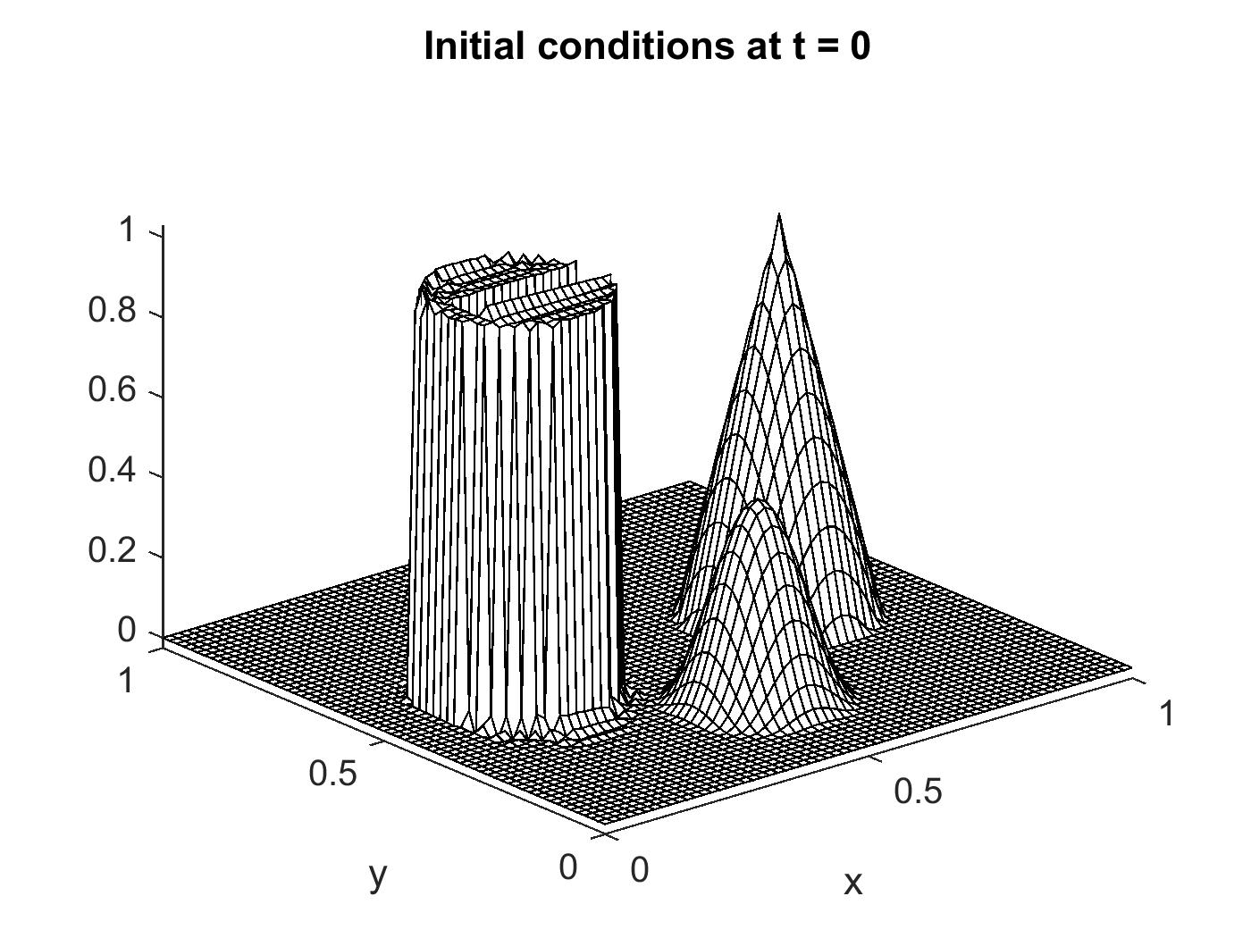
(a) Initial conditions

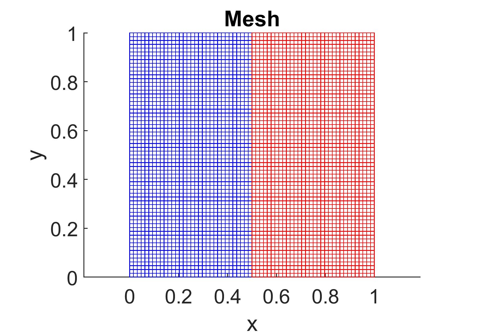
(b) Meshes used to discretize $\Omega_{1}$ (blue) and $\Omega_{2}$ (red)

Figure 2: Initial conditions and domain decomposition/mesh for our model 2D transmission problem

Suppose $\Omega$ is divided in half vertically by the line $x=0.5$, and let $\Omega_{1}$ and $\Omega_{2}$ denote the left and right side of the domain, respectively, as shown in Figure 2(b). Let $\gamma$ denote the interface $(x=0.5)$ between the two sides, and let $\Gamma_{i}=\partial\Omega_{i}\backslash\gamma$ for $i=1,2$. We take $\mathbf{n}_{\gamma}$ to be the unit normal on the interface pointing toward $\Omega_{2}$. In this section, we present select results for solving the model advection-diffusion interface problem (1) by performing both ROM-FEM and ROM-ROM coupling in the two subdomains, $\Omega_{1}$ and $\Omega_{2}$. The coupled ROM-FEM and ROM-ROM problems are solved by using the IVR partitioned schemes formulated in Section 4.2 and Section 4.3, respectively. We compare our ROM-FEM and ROM-ROM solutions to results obtained by employing our IVR partitioned scheme to perform FEM-FEM coupling between the two subdomains (see Section 3). For comparison purposes, we also include results obtained by building a global (uncoupled) FEM model as well as a global ROM in the full domain $\Omega$.

For the FEM discretizations, we employ a uniform spatial resolution of $\frac{1}{64}$ in both the $x$ and $y$ directions. The ROMs are developed from snapshots collected from a monolithic FEM discretization of $\Omega$ using the approach described in Section 4.1, with snapshots collected at intervals $\Delta_{s}t=1.35\times 10^{-2}$ and $\Delta_{s}t=6.73\times 10^{-3}$ for the pure advection and high Peclét variants of our test case, respectively. These snapshot selection strategies yield 466 and 933 snapshots for the two problem variants, respectively. All ROMs evaluated herein are run in the reproductive regime, that is, with the same parameter values, boundary conditions and initial conditions as those used to generate the snapshot set from which these models were constructed; predictive ROM simulations will be considered in a subsequent publication. In general, between 20-25 modes are needed to capture 90% of the snapshot energy and between 50-65 modes are needed to capture 99.999% of the snapshot energy for both problem variants, where the snapshot energy fraction is defined as $1-\delta$. As noted in Section 4.3, for the ROM-ROM couplings, we allow the bases in $\Omega_{1}$ and $\Omega_{2}$ to have different numbers of modes, denoted by $N_{R,\text{left}}$ and $N_{R,\text{right}}$, respectively. Hence, the number of modes required to capture a given snapshot energy fraction varies slightly between the two subdomains. All simulations are performed using an explicit 4th order Runge-Kutta (RK4) scheme with time-step $\Delta t=3.37\times 10^{-3}$, the time-step computed by the Courant-Friedrichs-Lewy (CFL) condition for this problem.

In the results below, we report for the various models evaluated the following relative errors as a function of the basis size and the total online CPU time:

$$\epsilon:=\frac{||X_{2\pi}-F_{2\pi}||_{2}}{||F_{2\pi}||_{2}}.$$ (18)

In (18), $X\in\{R,FF,RF,RR\}$, where $R$ denotes the global ROM solution computed in all of $\Omega$, $FF$ denotes a FEM-FEM coupled solution, $RF$ denotes a ROM-FEM coupled solution, and $RR$ denotes a ROM-ROM coupled solution. The subscripts in (18) denote the time at which a given solution is evaluated, i.e., $RF_{2\pi}$ is the ROM-FEM solution at time $t=2\pi$. The reference solution in (18), denoted by $F_{2\pi}$, is the global FEM solution computed in all of $\Omega$ at time $t=2\pi$. For the pure advection problem, we additionally report:

$$\epsilon_{0}:=\frac{||X_{0}-X_{2\pi}||_{2}}{||X_{2\pi}||_{2}},$$ (19)

for $X\in\{F,R,FF,RF,RR\}$. As shown in (maxnames[23], Leveque_96_SINUM), for the exact solution to the pure advection problem, $\epsilon_{0}$ is identically zero.

First, in Figure 3, we plot the relative error $\epsilon$ in (18) as a function of the POD basis size for the various couplings and the two problem variants considered herein. All errors are calculated with respect to the global FEM solution computed in all of $\Omega$. For the ROM-ROM couplings, the basis size in Figure 3 is obtained by calculating the average of the basis sizes in $\Omega_{1}$ and $\Omega_{2}$, denoted by $N_{R,\text{left}}$ and $N_{R,\text{right}}$ respectively. The reader can observe that all models exhibit convergence with respect to the basis size. In particular, the ROM-FEM and ROM-ROM solutions converge at a rate of approximately two. For the pure advection problems, the ROM-FEM and ROM-ROM solutions appear to be approaching the FEM-FEM error with basis refinement, and the ROM-ROM solution appears to be converging to the ROM-FEM solution. It is interesting to observe that the global ROM solutions achieve a greater accuracy than the FEM-FEM coupled solutions. Moreover, for the high Peclét version of the problem, the ROM-FEM coupled solution can achieve an accuracy that is slightly better than the FEM-FEM coupled solution. This behavior is likely due to the fact that the ROM solution was created using snapshots from a global FEM solution, which is more accurate than the coupled FEM-FEM solution.

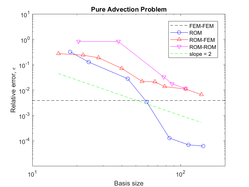
(a) Pure Advection

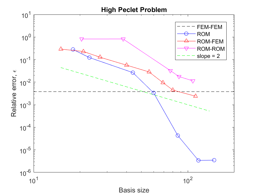
(b) High Peclét

Figure 3: Relative errors (18) with respect to the global FEM solution as a function of the POD basis size for different discretizations of the pure advection (a) and high Peclét (b) variants of our model transmission problem.

In evaluating the viability of a reduced model, it is important to consider not only the model’s accuracy, but also its efficiency. Toward this effect, Figures 4(a) and (b) show Pareto plots for the models evaluated on the pure advection and high Peclét problems, respectively. In these figures, we plot the relative errors (18) as a function of the total online CPU time. As expected, the global FEM and FEM-FEM models require the largest CPU time, followed by the ROM-FEM models, the ROM-ROM models and the global ROM models. It is interesting to remark that the FEM-FEM discretizations are actually slightly faster than the global FEM discretizations. This suggests that, in the case of high-fidelity models, our proposed coupling approach does not introduce any significant overhead. While the global ROM achieves the most accurate solution in the shortest amount of time, we are targeting here the scenario where the analyst does not have access to a single domain solver, and is forced to couple models calculated independently in different parts of the computational domain. The results in Figure 4 show that, by introducing ROM-FEM and ROM-ROM coupling, one can reduce the CPU time by 1-1.5 orders of magnitude without sacrificing accuracy.

(a) Pure Advection

(b) High Peclét

Figure 4: Pareto plot (relative errors (18) as a function of the total online CPU time) for different discretizations of the pure advection (a) and high Peclét (b) variants of our model transmission problem.

Turning our attention now to the pure advection problem, we plot in Figure 5 the relative errors $\epsilon_{0}$ in (19) as a function of the basis size. Again, the global FEM model is the most

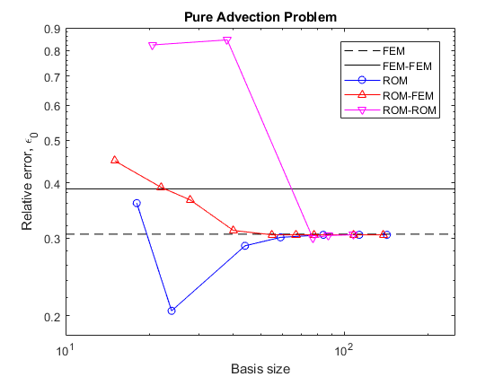
Figure 5: Relative errors (19) as a function of the POD basis size for different discretizations of the pure advection problem.

accurate, followed by the FEM-FEM, the ROM-FEM and the ROM-ROM models. It is interesting to observe that the global ROM surpasses the global FEM solution when it comes to accuracy for certain (intermediate) basis sizes. The primary takeaway from Figure 5 is that the ROM-FEM, the ROM-ROM and the global ROM solutions asymptotically approach the global FEM solution as the basis size is refined. This provides further verification for the models evaluated, in particular, for our new IVR coupling approach.

Next, in Figure 6, we plot some representative ROM-FEM and ROM-ROM solutions to the high Peclét variant of the targeted problem at the final simulation time $2\pi$. Also plotted is the single domain global FEM solution computed for this problem. The reader can observe that all three solutions are indistinguishable from one another. Figure 7 plots the ROM-FEM and ROM-ROM solutions to the high Peclét problem along the interface $\Gamma$ for each of the subdomains at the final simulation time $2\pi$. It can be seen from this figure that the solutions in $\Omega_{1}$ and $\Omega_{2}$ match incredibly well along the interface boundary. This suggests that our coupling method has not introduced any spurious artifacts into the discretization. We omit plots analogous to Figures 6 and 7 for the pure advection problem for the sake of brevity, as they lead to similar conclusions as high Peclét problem results.

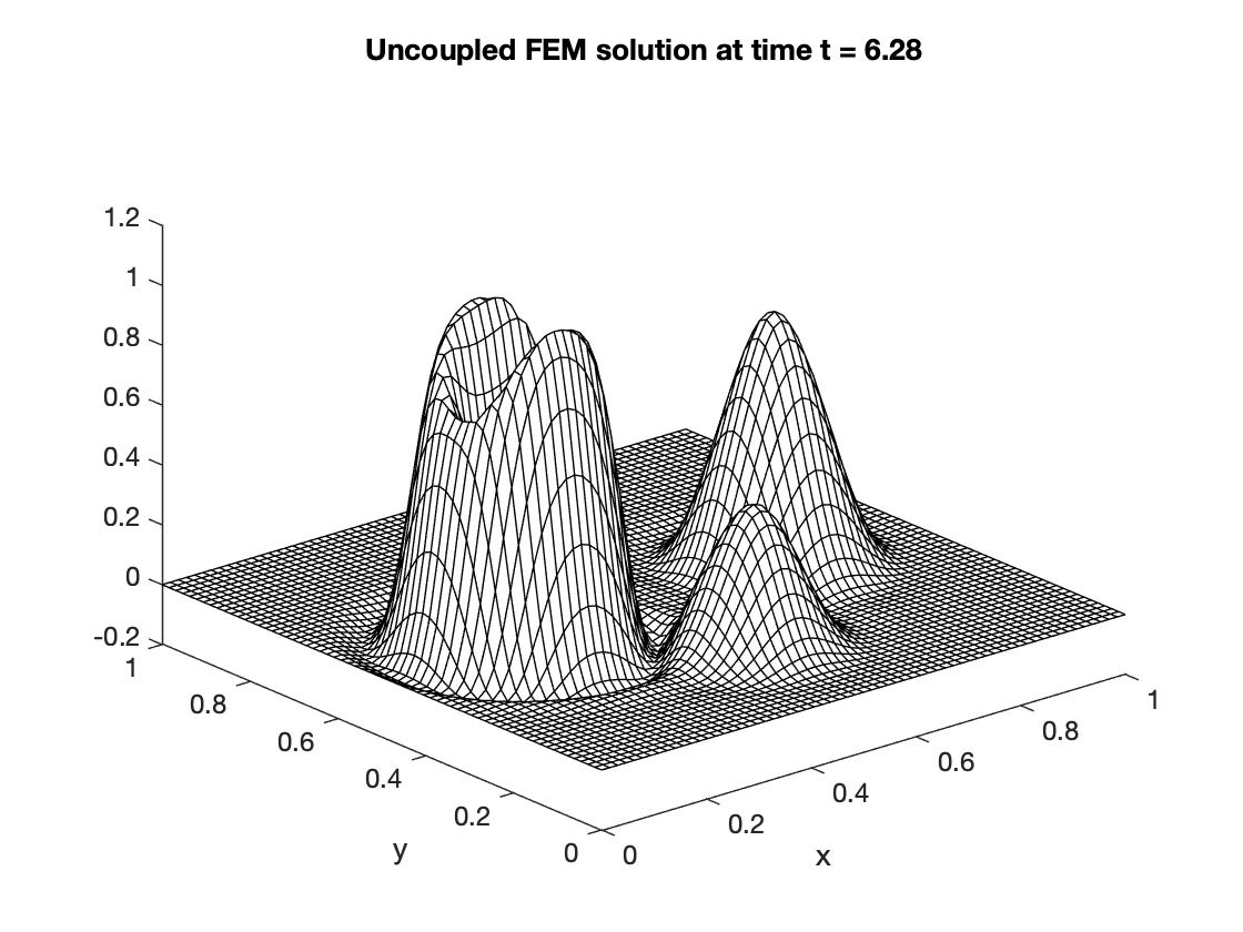
(a) Global FEM

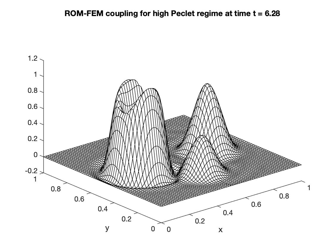
(b) ROM-FEM ($N_{R}=80$)

(c) ROM-ROM ($N_{R,\text{left}}=112$, $N_{R,\text{right}}=110$)

Figure 6: Comparison of global FEM, ROM-FEM and ROM-ROM solutions for the high Peclét variant of our model transmission problem at the final simulation time $t=2\pi$.

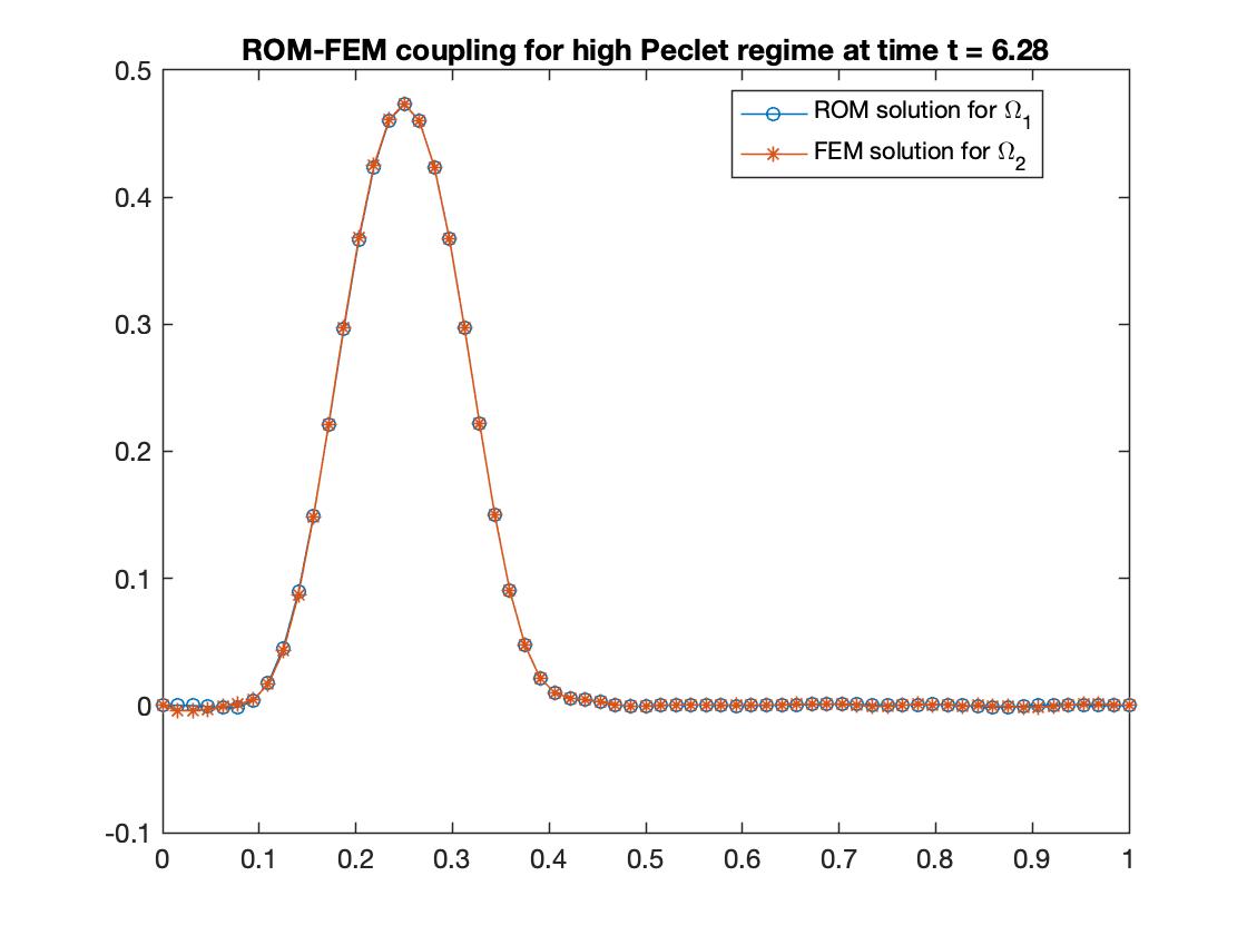
(a) ROM-FEM ($N_{R}=80$)

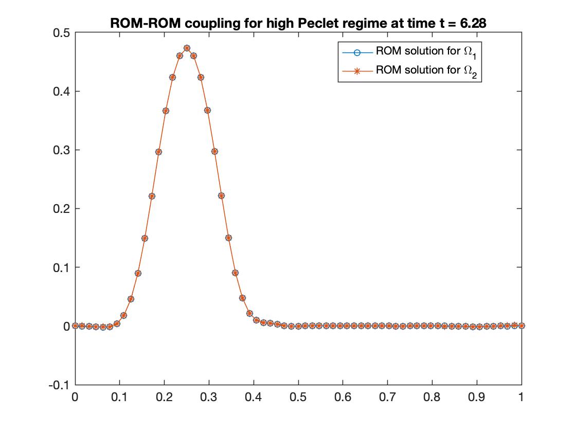
(b) ROM-ROM ($N_{R,\text{left}}=112$, $N_{R,\text{right}}=110$)

Figure 7: Comparison of the interface ROM-FEM and ROM-ROM solutions for high Peclét variant of our model transmission problem at the final simulation time $t=2\pi$.

CONCLUSIONS

We presented an explicit partitioned scheme for a transmission problem that extends the approach developed in (maxnames[28], AdC:CAMWA) to the case of coupling a projection-based ROM with a traditional finite element scheme and/or with another projection-based ROM. In particular, the scheme begins with a monolithic formulation of the transmission problem and then employs a Schur complement to solve for a Lagrange multiplier representing the interface flux as a Neumann boundary condition. We constructed a ROM from a full finite element solution and then presented an algorithm to couple this reduced model with either a traditional finite element scheme or another reduced model. Our numerical results show that the ROM-FEM and ROM-ROM coupling produces solutions which strongly agree with those produced by a global FEM solver. Additionally, implementing the ROM in one or more subdomains reduces the time and computational cost of solving the coupled system. In principle, this coupling method should extend to other discretizations such as finite volume, and the case of multiple ($>2$) subdomains; these scenarios will be studied in future work. Additionally, extensions to nonlinear and multiphysics problems, as well as predictive runs will be considered.

REFERENCES

- [1] A. Ammar, F. Chinestra and E. Cueto “Coupling finite elements and proper generalized decompositions” In International Journal for Multiscale Computational Engineering 9, 2011, pp. 17–33
- [2] H. Antil, M. Heinkenschloss, R. Hoppe and D. Sorensen “Domain decomposition and model reduction for the numerical solution of PDE constrained optimization problems with localized optimization variables” In Computing and Visualization in Science 13, 2010, pp. 249–264
- [3] Nadine Aubry, Philip Holmes, John L. Lumley and Emily Stone “The dynamics of coherent structures in the wall region of a turbulent boundary layer” In Journal of Fluid Mechanics 192 Cambridge University Press, 1988, pp. 115–173 DOI: 10.1017/S0022112088001818
- [4] Joan Baiges, Ramon Codina and Sergio R. Idelsohn “A domain decomposition strategy for reduced order models. Application to the incompressible Navier–Stokes equations” In Computer Methods in Applied Mechanics and Engineering 267, 2013, pp. 23–42
- [5] J.W. Banks, W.D. Henshaw, D.W. Schwendeman and Qi Tang “A stable partitioned FSI algorithm for rigid bodies and incompressible flow. Part I: Model problem analysis” In Journal of Computational Physics 343, 2017, pp. 432–468 DOI: https://doi.org/10.1016/j.jcp.2017.01.015
- [6] Greg C. Bessette, Courtenay T. Vaughan, Raymond L. Bell and Stephen W. Attaway “Modeling Air Blast on Thin-shell Structures with Zapotec” In Proceedings of the 74 th Shock and Vibration Symposium, 2003
- [7] Pavel Bochev and R.. Lehoucq “On the Finite Element Solution of the Pure Neumann Problem” In SIAM Review 47.1 SIAM, 2005, pp. 50–66 DOI: 10.1137/S0036144503426074
- [8] M. Buffoni, H. Telib and A. Iollo “Iterative Methods for Model Reduction by Domain Decomposition”, 2007
- [9] D. Cinquegrana, A. Viviani and R. Donelli “A hybrid method based on POD and domain decomposition to compute the 2-D aerodynamic flow field - incompressible validation”, 2011, pp. AIMETA 2011–XX Congresso dell’Associazione Italiana di Meccanica Teorica e Applicata\bibrangessepBologna\bibrangessepITA
- [10] A. Corigliano, M. Dossi and S. Mariani “Model Order Reduction and domain decomposition strategies for the solution of the dynamic elastic–plastic structural problem” In Computer Methods in Applied Mechanics and Engineering 290.C, 2015, pp. 127–155
- [11] Alberto Corigliano, Martino Dossi and Stefano Mariani “Domain decomposition and model order reduction methods applied to the simulation of multi-physics problems in MEMS” Computational Fluid and Solid Mechanics 2013 In Computers & Structures 122, 2013, pp. 113–127
- [12] A. de Boer, A.H. Zuijlen and H. Bijl “Review of coupling methods for non-matching meshes” Domain Decomposition Methods: recent advances and new challenges in engineering In Computer Methods in Applied Mechanics and Engineering 196.8, 2007, pp. 1515–1525 DOI: http://dx.doi.org/10.1016/j.cma.2006.03.017
- [13] Jens L. Eftang and Anthony T. Patera “Port reduction in parametrized component static condensation: approximation and a posteriori error estimation” In International Journal for Numerical Methods in Engineering 96.5, 2013, pp. 269–302
- [14] Jens L. Eftang and Anthony T. Patera “A port-reduced static condensation reduced basis element method for large component-synthesized structures: approximation and A Posteriori error estimation” In Advanced Modeling and Simulation in Engineering Sciences 1.3, 2014
- [15] B. Gatzhammer “Efficient and Flexible Partitioned Simulation of Fluid-Structure Interactions”, 2014
- [16] Max D. Gunzburger, Janet S. Peterson and John N. Shadid “Reduced-order modeling of time-dependent PDEs with multiple parameters in the boundary data” In Computer Methods in Applied Mechanics and Engineering 196, 2007, pp. 1030–1047
- [17] Chi Hoang, Youngsoo Choi and Kevin Carlberg “Domain-decomposition least-squares Petrov–Galerkin (DD-LSPG) nonlinear model reduction” In Computer Methods in Applied Mechanics and Engineering 384, 2021, pp. 113997
- [18] P. Holmes, J. Lumpley and G. Berkooz “Turbulence, Coherent structures, dynamical systems and symmetry” Cambridge University Press, 1996
- [19] L. Iapichino, A. Quarteroni and G. Rozza “Reduced basis method and domain decomposition for elliptic problems in networks and complex parametrized geometries” In Computers & Mathematics with Applications 71.1, 2016, pp. 408–430
- [20] P. Kerfriden, O. Goury, T. Rabczuk and S.P.A. Bordas “A partitioned model order reduction approach to rationalise computational expenses in nonlinear fracture mechanics” In Computer Methods in Applied Mechanics and Engineering 256, 2013, pp. 169–188
- [21] P. LeGresley “Application of Proper Orthogonal Decomposition (POD) to Design Decomposition Methods”, 2005
- [22] P. LeGresley and J. Alonso “Dynamic domain decomposition and error correction for reduced order models”, 2003, pp. 41st Aerospace Sciences Meeting and Exhibit\bibrangessepReno\bibrangessepNevada
- [23] Randall J. LeVeque “High-Resolution Conservative Algorithms for Advection in Incompressible Flow” In SIAM Journal on Numerical Analysis 33.2 SIAM, 1996, pp. 627–665 DOI: 10.1137/0733033
- [24] D. Lucia, P. King, P. Beran and M. Oxley “Reduced order modeling for a one-dimensional nozzle flow with moving shocks”, 2001, pp. 15th AIAA Computational Fluid Dynamics Conference\bibrangessepAnaheim\bibrangessepCA
- [25] David J. Lucia, Paul I. King and Philip S. Beran “Reduced order modeling of a two-dimensional flow with moving shocks” In Computers & Fluids 32.7, 2003, pp. 917–938
- [26] Y. Maday and E. Ronquist “The reduced basis element method: application to a thermal fin problem” In SIAM J. Sci. Comput. 26.1, 2004, pp. 240–258
- [27] I. Maier and B. Haasdonk “A Dirichlet-Neumann reduced basis method for homogeneous domain decomposition problems” In Applied Numerical Mathematics 78, 2014, pp. 31–48
- [28] K. Peterson, P. Bochev and P. Kuberry “Explicit synchronous partitioned algorithms for interface problems based on Lagrange multipliers” In Computers & Mathematics with Applications 78, 2019, pp. 459–482
- [29] Serge Piperno and Charbel Farhat “Partitioned procedures for the transient solution of coupled aeroelastic problems – Part II: energy transfer analysis and three-dimensional applications” Advances in Computational Methods for Fluid-Structure Interaction In Computer Methods in Applied Mechanics and Engineering 190.24–25, 2001, pp. 3147–3170 DOI: http://dx.doi.org/10.1016/S0045-7825(00)00386-8
- [30] A. Radermacher and S. Reese “Model reduction in elastoplasticity: proper orthogonal decomposition combined with adaptive sub-structuring” In Computational Mechanics 54, 2014, pp. 677–687
- [31] Glenn Randers-Pehrson and Kenneth A. Bannister “Airblast Loading Model for DYNA2D and DYNA3D”, 1997
- [32] L. Sirovich “Turbulence and the dynamics of coherent structures, Part III: dynamics and scaling” In Quarterly of Applied Mathematics 45.3 Brown University, 1987, pp. 583–590 URL: http://www.jstor.org/stable/43637459
- [33] K. Sockwell et al. “Interface Flux Recovery coupling method for the ocean–atmosphere system” In Results in Applied Mathematics 8, 2020, pp. 100–110