The role of electromagnetic gauge-field fluctuations in the selection between chiral and nematic superconductivity

Abstract

Motivated by the observation of nematic superconductivity in several systems, we revisit the problem of the leading pairing instability of two-component unconventional superconductors on the triangular lattice – such as $\left(p_{x},\,p_{y}\right)$-wave and $\left(d_{x^{2}-y^{2}},\,d_{xy}\right)$-wave. Such a system has two possible superconducting states: the chiral state (e.g. $p+ip$ or $d+id$), which breaks time-reversal symmetry, and the nematic state (e.g. $p+p$ or $d+d$), which breaks the threefold rotational symmetry of the lattice. Weak-coupling calculations generally favor the chiral over the nematic superconducting state, raising the question of what mechanism can stabilize the latter. Here, we show that the electromagnetic field fluctuations can play a crucial role in selecting between these two states. Specifically, we derive and analyze the effective free energy for the two-component superconducting order parameter after integrating out the gauge-field fluctuations, which is formally justified if the spatial order parameter fluctuations can be neglected. A non-analytic cubic term arises, as in the case of a conventional $s$-wave superconductor. However, unlike the latter, the cubic term depends on the relative phase and on the relative amplitudes between the two order parameter components, in such a way that it generally favors the nematic state. This result is a direct consequence of the fact that the stiffness of the superconducting order parameter is not isotropic. Competition with the quartic term, which favors the chiral state, leads to a renormalized phase diagram in which the nematic state displaces the chiral state over a wide region in the parameter space. We analyze the stability of the fluctuation-induced nematic phase, generalize our results to tetragonal lattices, and discuss their applicability to candidate nematic superconductors, including twisted bilayer graphene.

I Introduction

A nematic superconductor spontaneously breaks not only the $U(1)$ gauge symmetry, but also a discrete rotational symmetry of the system, thus lowering the symmetry of the point group that characterizes the underlying lattice. Recent experiments have reported evidence of rotational symmetry-breaking superconducting states in different quantum materials, such as doped Bi₂Se₃ [1, 2, 3, 4], few-layer NbSe₂ [5, 6], the topological semimetal CaSn₃ [7], and the iron-based superconductors Ba_1-xK_xFe₂As₂ [8] and LiFeAs [9]. There is a longer list of materials in which superconductivity can coexist with nematic order, such as the iron chalcogenide FeSe [10] or the nickel arsenide BaNi₂As₂ [11], but in these cases the superconducting state emerges in the presence of a nematically ordered state that onsets at much higher temperatures [12]. Interestingly, the recently discovered twisted bilayer graphene [13, 14, 15, 16] has also been reported to display a nematic superconducting state in the “hole-doped” side of the phase diagram, as indicated by the in-plane anisotropy of the critical magnetic field and of the critical current [17].

Theoretically, a nematic pairing state requires the simultaneous existence of (at least) two superconducting order parameters whose relative phase is not $\pi/2$. Generally, there are two different scenarios in which this can happen. In the first case, two independent order parameters, $\psi_{1}$ and $\psi_{2}$, condense at similar temperatures due to some fine tuning of the microscopic parameters involved [18]. One example is the $s+d$ state proposed in Ba_1-xK_xFe₂As₂ [19, 20]. In the second scenario, the superconducting order parameter has two symmetry-related components $\psi=\left(\psi_{1},\,\psi_{2}\right)$, i.e. it transforms as a two-dimensional irreducible representation (irrep) of the lattice point group. Examples of such order parameters include the $\left(p_{x},\,p_{y}\right)$-wave and $\left(d_{x^{2}-y^{2}},\,d_{xy}\right)$-wave in triangular lattices or the $\left(p_{x},\,p_{y}\right)$-wave and the $\left(d_{xz},\,d_{yz}\right)$-wave in tetragonal lattices [21]. Since this case does not require fine tuning, we will focus on it in the remainder of the paper.

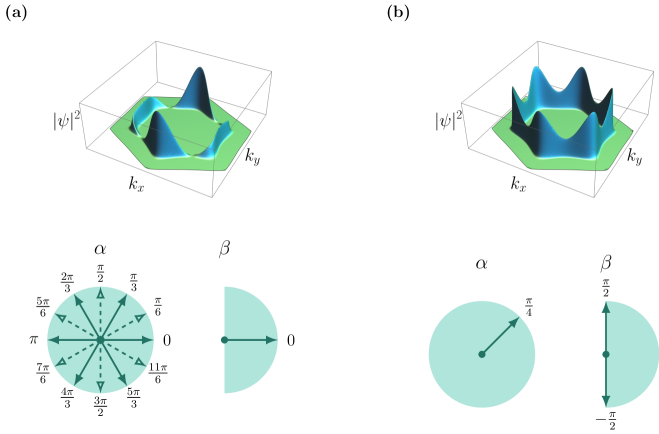
Figure 1: Plots of the superconducting gap function along a generic Fermi surface on the triangular lattice. The order parameter is parametrized in terms of three angles as $\psi=|\psi|e^{i\varphi}\left(\cos\alpha,e^{i\beta}\sin\alpha\right)$. In this figure, the two components of $\psi$ transform as $d_{x^{2}-y^{2}}$ and $d_{xy}$ waves ($E_{2}$ irrep of $D_{6}$). (a) The gap function in the nematic state, which lowers the $C_{6z}$ rotational symmetry of the lattice to $C_{2z}$, is obtained when $\alpha=\tfrac{n\pi}{6}$ [with even $n=0,2,..,10$ (solid arrows) or odd $n=1,3,...,11$ (dashed arrows)] and $\beta=0$. To produce this plot we chose $\alpha=0$. (b) The gap function in the chiral state is obtained when $\alpha=\tfrac{\pi}{4}$ and $\beta=\pm\tfrac{\pi}{2}$. It does not break any lattice symmetry. However, this state breaks time reversal symmetry.

It is convenient to parametrize $\psi$ in terms of three angles $\varphi\in[0,2\pi)$, $\beta\in\left[-\pi/2,\,\pi/2\right]$ and $\alpha\in[0,2\pi)$ as $\psi=|\psi|e^{i\varphi}\left(\cos{\alpha},e^{i\beta}\sin{\alpha}\right)$ [22]. Below the transition temperature $T_{c}$, the global phase $\varphi$ acquires a definite value and the $U(1)$ gauge symmetry is broken. As for $\alpha$, which describes the relative amplitudes between the two superconducting order parameters, and $\beta$, which describes the relative phase between $\psi_{1}$ and $\psi_{2}$, their allowed values are not continuous, but restricted to discrete sets by the symmetries of the system. In the particular case of the triangular (or honeycomb) lattice, there are two different possible sets of values [23]. The first one is $\beta=0$ and $\alpha=\tfrac{n\pi}{6}$ (with even $n=0,2,..,10$ or odd $n=1,3,...,11$), which corresponds to a nematic superconducting state. Fig. 1(a) shows the absolute value square of the gap ($\left|\psi\right|^{2}$) in the nematic phase, which clearly breaks the threefold rotational symmetry $C_{3z}$ of the lattice. Note that there are points in which $\left|\psi\right|^{2}=0$, corresponding to gap nodes. The different values of $\alpha$ correspond to the different ways of breaking the $C_{3z}$ symmetry. The second set of allowed values corresponds to $\alpha=\tfrac{\pi}{4}$ and $\beta=\pm\tfrac{\pi}{2}$. Because $\psi^{*}\neq\psi$, time-reversal symmetry is broken, and the superconducting state is chiral. In this situation, $\left|\psi\right|^{2}$ respects the threefold rotational symmetry of the lattice and is never zero, as shown in Fig. 1(b).

The key question is which microscopic mechanisms are responsible for the selection between the two possible pairing states – nematic or chiral. An argument usually invoked is that the chiral state should be favored, since it completely gaps out the Fermi surface [Fig. 1(b)], which would presumably maximize the condensation energy. In agreement with this expectation, weak-coupling calculations find that the chiral state is generally preferred [24, 25, 26, 27, 28] – unless spin-orbit coupling is significant [29]. Moreover, in noncentrosymmetric systems, time-reversal symmetry must be broken [30]. These results raise the interesting question of which mechanism stabilizes the nematic superconducting states that appear to be realized in the materials discussed above. Besides the aforementioned possibility of nearly degenerate single-component pairing states [31, 32, 33, 34], it has been pointed out that, in the case of a two-component superconductor, coupling to strong normal-state nematic or density-wave fluctuations can tip the balance in favor of nematic superconductivity [24, 19].

In this paper, we discuss another possible mechanism that does not require additional degrees of freedom or fine tuning. The key point is that, because the superconducting order parameter is charged, it couples to electromagnetic fluctuations. The effect of the gauge-field fluctuations on conventional $s$-wave superconductors has been widely investigated [35, 36, 37, 38, 39, 40]. The seminal work of Ref. [35] showed that, upon integrating out the gauge-field fluctuations, the superconducting transition becomes weakly first-order due to the emergence of a non-analytic negative cubic term in the free-energy expansion. Such an effect would be very small to be detected due to the narrow window in which fluctuations are important in $s$-wave superconductors. Because this procedure of integrating out the electromagnetic fields is formally justified only when the spatial order parameter fluctuations can be neglected, this conclusion is robust for type-I superconductors. For type-II superconductors, duality mappings and Monte Carlo simulations indicate that the transition remains second-order [36, 37, 39].

The role of gauge-field fluctuations on layered unconventional superconductors, where fluctuations generally can play a more prominent role than in conventional superconductors, has been less studied. Ref. [41] considered the case of a general multi-band superconductor with isotropic stiffness and found, like in the $s$-wave case, a fluctuation-induced first-order transition via a renormalization-group calculation. A similar result was found in Ref. [42] for a $p$-wave superconductor, and Ref. [43] reported the same outcome in the case of color superconductivity, where the gauge field is non-Abelian. Here, we extend this kind of perturbative analysis to the case of two-component superconductors in triangular and tetragonal lattices, taking into account the anisotropy of the superconducting stiffness introduced by the crystal lattice. Specifically, we integrate out the gauge-field fluctuations to obtain a renormalized Landau free-energy, which is then minimized.

Similarly to the $s$-wave [35] and isotropic unconventional superconductor cases [41, 42], we find a non-analytic cubic term with an overall negative sign, indicative of a first-order transition. However, the main difference is that this non-analytic term is not only dependent on $\left|\psi\right|^{3}$, but also on the angles $\alpha$ and $\beta$ that distinguish between the chiral and nematic states. This happens because the superconducting stiffness is not isotropic, as in the $s$-wave case. Interestingly, by combining numerical and analytical calculations, we find that the cubic contribution to the free-energy is always minimized for the nematic state. Consequently, because the chiral state arises from the minimization of quartic terms of the free energy, the nematic state becomes the global minimum of the renormalized free-energy in a wide region of the parameter-space where the chiral state was the global minimum of the mean-field free-energy. We further analyze the stability of this gauge-field-fluctuations induced nematic state as temperature is lowered below $T_{c}$. Finally, we discuss the limitations of our approach and the possible application of our results to twisted bilayer graphene and nematic superconductors in general.

The paper is organized as follows: we derive and solve the superconducting free-energy renormalized by electromagnetic field fluctuations in the case of a two-component superconductor on a triangular lattice in Sec. II. In Sec. III, we repeat the same procedure for the case of a tetragonal lattice. In Sec. IV, we summarize and discuss our results, presenting our concluding remarks. Appendix A presents additional details of the derivation of the renormalized free-energy.

II Two-component superconductor on the triangular lattice

We first consider a two-component unconventional superconductor on a lattice with threefold rotational symmetry in the presence of electromagnetic field fluctuations. This applies to the cases of twisted bilayer graphene, with a triangular moiré lattice and point group $D_{6}$, and to doped Bi₂Se₃ with a trigonal lattice and point group $D_{3d}$. Both of these groups admit two two-dimensional irreps corresponding to $p_{x}/p_{y}$-wave or $d_{x^{2}-y^{2}}/d_{xy}$-wave superconducting states – respectively, $E_{1}$ and $E_{2}$ in the case of $D_{6}$ and $E_{u}$ and $E_{g}$ in the case of $D_{3d}$. In all these cases, we parametrize the two-component superconducting order parameter $\psi$ as [22]:

$$\psi=|\psi|e^{i\varphi}\left(\cos\alpha,e^{i\beta}\sin\alpha\right)\mbox{,}$$ (1)

where $\alpha\in[0,2\pi)$ and $\beta\in\left[-\tfrac{\pi}{2},\tfrac{\pi}{2}\right]$. The global phase $\varphi$ can take any values in $[0,2\pi)$.

II.1 Renormalized free-energy functional

We now generalize the approach of Ref. [35] of integrating out the electromagnetic field fluctuations for the case of a two-component superconductor in a lattice with threefold rotational symmetry. Denoting by $\mathbf{A}$ the electromagnetic vector potential, and using the same notation as Ref. [35], the Ginzburg-Landau free-energy density has the form

$$\mathcal{F}\left[\psi,\mathbf{A}\right]=\mathcal{F}_{0}\left[\psi\right]+\mathcal{F}_{\mathrm{grad}}\left[\psi,\mathbf{A}\right]+\frac{1}{8\pi\mu_{0}}\left(\gradient\times\mathbf{A}\right)^{2}\mbox{,}$$ (2)

where $\mathcal{F}_{\mathrm{0}}\left[\psi\right]$ does not contain gradients of the superconducting order parameter and $\mathcal{F}_{\mathrm{grad}}\left[\psi,\mathbf{A}\right]$ contains all the symmetry allowed couplings between $\psi$ and $\mathbf{A}$. The last term is the free massless action of the gauge field. Here, $\mu_{0}$ is the magnetic permeability. The first term on the right-hand side of Eq. (2) is given by [21, 44, 23]

$$\mathcal{F}_{0} [\psi]=\frac{r}{2}|\psi|^{2}+\frac{u}{4}|\psi|^{4}+\frac{g}{4}\left[\left(\bar{\psi}\tau_{3}\psi\right)^{2}+\left(\bar{\psi}\tau_{1}\psi\right)^{2}\right]\mbox{,}$$ (3)

where $\tau_{i}$ refers to the Pauli matrices acting on the two-dimensional space of $\psi$ (with $i=1,2,3$ ) and $\bar{\psi}$ is the transposed complex conjugate of $\psi$. The parameter $r$ changes sign at the bare transition temperature $T_{0}$ as $r=r_{0}(T-T_{0})/T_{0}$, with $r_{0}>0$. Moreover, the conditions $u>0$ and $g+u>0$ must hold for $\mathcal{F}_{0}[\psi]$ to be bounded from below. In terms of the parametrization (1), we have:

$$\mathcal{F}_{0}[\psi]=\frac{r}{2}|\psi|^{2}+\frac{u}{4}|\psi|^{4}+\frac{g}{4}|\psi|^{4}\left(\sin^{2}2\alpha\cos^{2}\beta+\cos^{2}2\alpha\right).$$ (4)

To set the stage, we first review the mean-field results for the case in which gradient terms are absent – see, e.g., Ref. [21]. Minimizing $\mathcal{F}_{0}[\psi]$, the leading superconducting instabilities of Eq. (4) are either the nematic or the chiral state, both of which onset at $r<0$. Specifically when $g<0$, the leading superconducting state is nematic and the order parameter has the form $\psi\propto(\cos{\alpha},\sin{\alpha})$ with $\alpha\in[0,2\pi)$. When $g>0$, the leading superconducting state is chiral and $\psi\propto(1,\pm i)$. The mean-field phase diagram obtained from minimizing the free-energy in Eq. (4) is shown in Fig. 2. To this order in $\psi$, the Landau free-energy does not fix $\alpha$ to any particular value when the nematic state is the minimum. As we will discuss later, this continuous symmetry is lifted by sixth-order terms in the free-energy. For simplicity, here we neglect such sixth-order terms, since the quartic terms are enough to select between the nematic or the chiral state. In Sec. II.3 we discuss the role of the sixth-order terms in $\mathcal{F}_{\mathrm{0}}[\psi]$.

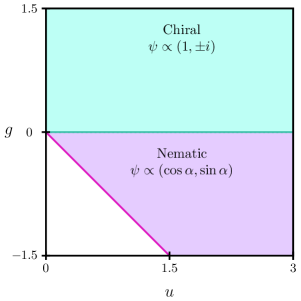
Figure 2: Mean-field phase diagram, in the $(u,g)$ parameter-space, for a two-component superconductor on a triangular lattice, based on the Landau free-energy expansion to quartic order in $\psi$ shown in Eq. (4). The white area in this plot corresponds to the regions in parameter-space where the free energy in Eq. (4) is unbounded.

The second term on the right-hand side of Eq. (2) consists of a sum of all symmetry allowed gradient terms that couple $\psi$ and $\mathbf{A}$ [21]:

$$\mathcal{F}_{\mathrm{grad}}[\psi,\mathbf{A}]=$$ (5)

$$K_{1}\left|D_{x}\psi_{1}+D_{y}\psi_{2}\right|^{2}+K_{2}\left|D_{x}\psi_{2}-D_{y}\psi_{1}\right|^{2}$$

$$+K_{3}\left(\left|D_{x}\psi_{1}-D_{y}\psi_{2}\right|^{2}+\left|D_{x}\psi_{2}+D_{y}\psi_{1}\right|^{2}\right)$$

$$+K_{4}\left(\left|D_{z}\psi_{1}\right|^{2}+\left|D_{z}\psi_{2}\right|^{2}\right)\mbox{,}$$

where $D_{x}=\partial_{x}-iq_{0}A_{x}$, etc. are the covariant derivatives and $q_{0}=2e/\hbar c$. The above $K_{i}$ parameters, known as stiffness coefficients, penalize spatial variations of the field in different directions. Importantly, the in-plane stiffness of the order parameter is not isotropic. We consider the situation in which the order parameter varies weakly in space whereas the electromagnetic fields vary more strongly. In this case, we can set $\gradient\psi=0$ in the expression above. This step is formally only justified for type-I superconductors, as explained in [35]. We will revisit this assumption in Sec. IV. With this assumption, the gradient terms simplify to:

$$\mathcal{F}_{\mathrm{grad}}[\psi,\mathbf{A}]= q_{0}^{2}\gamma_{0}\left|\psi\right|^{2}\left(\!A_{x}^{2}\!+\!A_{y}^{2}\right)\!+\!q_{0}^{2}\gamma_{3}(\bar{\psi}\tau_{3}\psi)\left(\!A_{x}^{2}\!-\!A_{y}^{2}\right)$$ (6)

$$+\!2A_{x}A_{y}q_{0}^{2}\gamma_{3}(\bar{\psi}\tau_{1}\psi)\!+\!A_{z}^{2}q_{0}^{2}\gamma_{z}\left|\psi\right|^{2}\mbox{,}$$

where we have defined the effective stiffness coefficients

$$\gamma_{z}=K_{4}\mbox{,}\quad\gamma_{0}=\frac{K_{1}+K_{2}+2K_{3}}{2}\quad\mbox{and}\quad\gamma_{3}=\frac{K_{1}-K_{2}}{2}.$$ (7)

In a layered quasi two-dimensional system, the magnitude of $\gamma_{z}$ should be much smaller than that of $\gamma_{0}$. However, as it will be clear later on, our result is not too sensitive to variations in $\gamma_{z}$.

To define the effective free-energy density of the single variable $\psi$, $\mathcal{F}_{\mathrm{eff}}[\psi]$, we take the trace over the physically allowed dynamic degrees of freedom of $\mathbf{A}$. In other words, the functional integral that defines $\mathcal{F}_{\mathrm{eff}}[\psi]$ is done over all the purely transverse configurations of the vector potential, $\mathbf{A}^{\perp}$,

$$e^{-\beta F_{\mathrm{eff}}[\psi]} =e^{-\beta F_{\mathrm{0}}[\psi]}$$ (8)

$$\times\int D\mathbf{A}^{\perp}\,e^{-\beta\int dV\{\mathcal{F}_{\mathrm{grad}}\left[\psi,\mathbf{A}\right]+\frac{1}{8\pi\mu_{0}}\left(\gradient\times\mathbf{A}\right)^{2}\}}\mbox{,}$$

where $\beta=1/\left(k_{B}T\right)$ and $F_{i}$ denotes the integrated free-energy density $\mathcal{F}_{i}$. It is convenient to proceed in the Coulomb gauge, $\nabla\cdot\mathbf{A}=0$, where the Fourier component of the vector potential that is parallel to the wave vector $\mathbf{k}$ vanishes,

$$\mathbf{A}_{\mathbf{k}}\cdot\hat{\mathbf{k}}=0.$$ (9)

To impose the above condition, we move to the spherical coordinate system $\mathbf{k}=k\left(\sin\theta\cos\phi,\sin\theta\sin\phi,\cos\theta\right)$ and consider the spherical basis formed by the unit vectors

$$\hat{\mathbf{k}} =\left(\sin\theta\cos\phi,\sin\theta\sin\phi,\cos\theta\right)\mbox{,}$$ (10)

$$\hat{\bm{\theta}} =\left(\cos\theta\cos\phi,\cos\theta\sin\phi,-\sin\theta\right)\,,$$

$$\hat{\bm{\phi}} =\left(-\sin\phi,\cos\phi,0\right)\mbox{.}$$

In this new basis, the Fourier components $\mathbf{A}_{\mathbf{k}}$ are denoted as

$$\mathbf{A}_{\mathbf{k}} =\vphantom{\int}A_{k\mathbf{k}}\hat{\mathbf{k}}+\vphantom{\int}A_{\theta\mathbf{k}}\hat{\bm{\theta}}+A_{\phi\mathbf{k}}\hat{\bm{\phi}}\mbox{, }$$ (11)

in terms of which the transverse component of the electromagnetic field becomes simply $\mathbf{A}_{\mathbf{k}}^{\perp}=\left(A_{\theta\mathbf{k}},A_{\phi\mathbf{k}}\right).$ Thus, in the Cartesian basis, the Fourier components $\mathbf{A}_{\mathbf{k}}$ are given by:

$$\begin{pmatrix}A_{x\mathbf{k}}\\ A_{y\mathbf{k}}\\ A_{z\mathbf{k}}\end{pmatrix}=\begin{pmatrix}\cos\theta\cos\phi A_{\theta\mathbf{k}}-\sin\phi A_{\phi\mathbf{k}}\\ \cos\theta\sin\phi A_{\theta\mathbf{k}}+\cos\phi A_{\phi\mathbf{k}}\\ -\sin\theta A_{\theta\mathbf{k}}\end{pmatrix}\mbox{,}$$ (12)

As a result, Eq. (8) can be written in terms of $A_{\theta\mathbf{k}}$ and $A_{\phi\mathbf{k}}$ as

$$e^{-\beta F_{\mathrm{eff}}[\psi]} =e^{-\beta F_{\mathrm{0}}[\psi]}\int D\mathbf{A}^{\perp}\,e^{-\tfrac{\beta\psi_{s}^{2}}{8\pi\mu_{0}}\int d^{3}k\,\mathbf{A}_{\mathbf{k}}^{\perp}\mathbf{M}_{\mathbf{k}}\mathbf{A}_{\mathbf{k}}^{\perp T}}\mbox{,}$$ (13)

where we have defined $\psi_{s}^{2}=8\pi\gamma_{0}q_{0}^{2}\mu_{0}|\psi|^{2}$ and $\mathbf{M}_{\mathbf{k}}$ is a $2\times 2$ matrix with components

$$\left(\mathbf{M}_{\mathbf{k}}\right)_{\theta\theta} =\cos^{2}\!\theta\left(1\!-\!\tfrac{\gamma_{z}}{\gamma_{0}}\!+\!\tfrac{\gamma_{3}}{\gamma_{0}}\cos 2\alpha\cos 2\phi\!+\!\tfrac{\gamma_{3}}{\gamma_{0}}\cos\beta\sin 2\alpha\sin 2\phi\right)\!+\!\tfrac{\gamma_{z}}{\gamma_{0}}\!+\!\tfrac{k^{2}}{\psi_{s}^{2}}\>\mbox{,}$$ (14)

$$\left(\mathbf{M}_{\mathbf{k}}\right)_{\phi\phi} =1-\tfrac{\gamma_{3}}{\gamma_{0}}\left(\cos 2\alpha\cos 2\phi+\cos\beta\sin 2\alpha\sin 2\phi\right)+\tfrac{k^{2}}{\psi_{s}^{2}}\>\mbox{,}$$

$$\left(\mathbf{M}_{\mathbf{k}}\right)_{\theta\phi} =\left(\mathbf{M}_{\mathbf{k}}\right)_{\phi\theta}=\tfrac{\gamma_{3}}{\gamma_{0}}\cos\theta\left(\cos\beta\sin 2\alpha\cos 2\phi-\cos 2\alpha\sin 2\phi\right)\>\mbox{.}$$

Thus, $\tfrac{\beta\psi_{s}^{2}}{8\pi\mu_{0}}\mathbf{M}_{\mathbf{k}}$ is the “mass matrix” of the gauge field. Above the superconducting transition, where the superconducting order parameter $\psi_{s}$ is zero, the mass matrix has zero determinant, indicative of a massless field. For a non-zero $\psi_{s}$, the functional integral in Eq. (13) only converges if both eigenvalues of the matrix $\mathbf{M}_{\mathbf{k}}$ are positive, i.e., if the gauge field becomes massive. The conditions for this to happen are that both $\gamma_{0}$ and $\gamma_{z}$ should be positive and $|\gamma_{3}|<\gamma_{0}$.

The result of the functional integration over all physical configurations of $\mathbf{A}$ gives the effective free-energy density functional for $\psi$, which is a sum of two terms

$$\mathcal{F}_{\mathrm{eff}}\left[\psi\right] =\mathcal{F}_{\mathrm{0}}\left[\psi\right]+\mathcal{F}_{\mathrm{EM}}[\psi]\mbox{.}$$ (15)

The first term, $\mathcal{F}_{\mathrm{0}}[\psi]$, was defined in Eqs. (3) or (4) whereas the second term $\mathcal{F}_{\mathrm{EM}}[\psi]$ is given by the result of the Gaussian integration over the electromagnetic fields:

$$\mathcal{F}_{\mathrm{EM}}[\psi]=\frac{4T\Lambda^{3}}{3(2\pi)^{2}}\ln\left(\psi_{s}\right)$$ (16)

$$+\frac{T\psi_{s}^{3}}{2(2\pi)^{3}}\int_{0}^{2\pi}d\phi\int_{-1}^{1}dx\int_{0}^{\tfrac{\Lambda}{\psi_{s}}}dq\,q^{2}\ln\left(c+bq^{2}+q^{4}\right)\mbox{.}$$

In Eq. (16), we performed a change of variables to $x=\cos\theta$ and $q=k/\psi_{s}$. Here, $\Lambda$ is the momentum cutoff and the polynomial $c+bq^{2}+q^{4}=\det\mathbf{M}_{\mathbf{k}}$. The dimensionless quantities $b$ and $c$ are given by

$$\!b= \frac{\gamma_{z}}{\gamma_{0}}+1+\left(1-\frac{\gamma_{z}}{\gamma_{0}}\right)x^{2}$$ (17)

$$-\frac{\gamma_{3}}{\gamma_{0}}\left(1-x^{2}\right)\left(\cos 2\alpha\cos 2\phi+\cos\beta\sin 2\alpha\sin 2\phi\right)\,,$$

$$\!c= \frac{\gamma_{z}}{\gamma_{0}}\!+\!\left[1-\frac{\gamma_{z}}{\gamma_{0}}-\left(\frac{\gamma_{3}}{\gamma_{0}}\right)^{2}\left(\cos^{2}\beta\sin^{2}2\alpha+\cos^{2}2\alpha\right)\right]\!x^{2}\!$$

$$-\frac{\gamma_{z}\gamma_{3}}{\gamma_{0}^{2}}\left(1-x^{2}\right)\left(\cos 2\alpha\cos 2\phi+\cos\beta\sin 2\alpha\sin 2\phi\right).$$

In order to extract from $\mathcal{F}_{\mathrm{EM}}[\psi]$ the leading terms in the order parameter, it is necessary to Taylor expand the logarithm before integrating. After defining

$$a_{\pm}^{2}=\frac{b}{2}\pm\frac{\sqrt{b^{2}-4c}}{2}$$ (18)

we rewrite the integral $\mathcal{F}_{\mathrm{EM}}[\psi]$ as an infinite sum (see Appendix A for details)

$$\mathcal{F}_{\mathrm{EM}}[\psi]=-\frac{T\psi_{s}^{3}}{48\pi^{2}}\int_{0}^{2\pi}d\phi\int_{-1}^{1}dx\left(a_{+}^{3}+a_{-}^{3}\right)$$ (19)

$$\!\!\!+\sum_{n=1}^{\infty}\frac{T\psi_{s}^{2n}}{2(2\pi)^{3}}\int_{0}^{2\pi}d\phi\int_{-1}^{1}dx\frac{(-1)^{n-1}\Lambda^{-2n+3}}{n(-2n+3)}\left(a_{+}^{2n}+a_{-}^{2n}\right).$$

The series that contains even powers of $\psi_{s}$, i.e. $\psi_{s}^{2n}$, simply renormalizes the existing analytic terms in the bare Landau free-energy. For $n>1$, these corrections are small due to the cutoff pre-factor $\Lambda^{-2n+3}$. For $n=1$, the correction is independent of the angles $\alpha$ and $\beta$ and results in a renormalization of the bare transition temperature $T_{0}$. Therefore, hereafter, we ignore the infinite series and focus only on the cubic term of Eq. (19):

$$\mathcal{F}_{\mathrm{EM}}[\psi]=- \frac{T\psi_{s}^{3}}{48\pi^{2}}\int_{0}^{2\pi}d\phi\int_{-1}^{1}dx\,\left(a_{+}^{3}+a_{-}^{3}\right).$$ (20)

The above cubic term is a non-analytic function of $\psi$. Non-analytic contributions to the Ginzburg-Landau free-energy are generally expected to arise when a massless field is integrated out – see for instance the case of nematic order parameters coupling to acoustic phonon modes [45, 46, 47, 48]. If we set $\gamma_{3}=0$ and $\gamma_{0}=\gamma_{z}$, it follows that $b=2$ and $c=1$, such that $a_{+}=a_{-}=1$. In this case, Eq. (20) gives a cubic term with a negative coefficient, as in the case of an $s$-wave superconductor [35]. What makes our case different from the $s$-wave case is the additional stiffness coefficient $\gamma_{3}$, which is absent for a single-component superconductor, and which makes $\mathcal{F}_{\mathrm{EM}}[\psi]$ depend on the relative angles $\alpha$ and $\beta$.

We first analyze numerically the dependence of the cubic term $\mathcal{F}_{\mathrm{EM}}[\psi]$ on $\alpha$ and $\beta$. It is convenient to express the cubic term in terms of the dimensionless integral $f^{(3)}$ that depends only on the ratios between the stiffness coefficients $\frac{\gamma_{3}}{\gamma_{0}}$ and $\frac{\gamma_{z}}{\gamma_{0}}$ and on the angles $\alpha$ and $\beta$:

$$\mathcal{F}_{\mathrm{EM}}[\psi]=\frac{T\psi_{s}^{3}}{12\pi}\,f^{(3)}\left(\frac{\gamma_{3}}{\gamma_{0}},\frac{\gamma_{z}}{\gamma_{0}},\alpha,\beta\right)\mbox{.}$$ (21)

with:

$$f^{(3)}\equiv-\frac{1}{4\pi}\int_{0}^{2\pi}d\phi\int_{-1}^{1}dx\,\left(a_{+}^{3}+a_{-}^{3}\right)$$ (22)

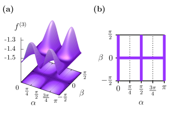
Figure 3: (a) Plot of $f^{(3)}\left(\tfrac{\gamma_{3}}{\gamma_{0}},\tfrac{\gamma_{z}}{\gamma_{0}},\alpha,\beta\right)$ for fixed $\tfrac{\gamma_{3}}{\gamma_{0}}=0.8$ and $\tfrac{\gamma_{z}}{\gamma_{0}}=0.1$ as a function of $\alpha$ and $\beta$. (b) Location of the minima on the $(\alpha,\beta)$ plane. The minima correspond to a nematic state with order parameter $\psi\propto(\cos\alpha,\sin\alpha)$, where $\alpha$ is not fixed to be any particular value.

We analyzed $f^{(3)}$ by plotting it as a function of $\alpha$ and $\beta$ for varying $\gamma_{z}/\gamma_{0}\in[0,1]$ and $\gamma_{3}/\gamma_{0}\in[-1,1]$. In all cases we studied, we found $f^{(3)}<0$, like the simpler case of the $s$-wave superconductor treated in [35]. More importantly, the minima of $f^{(3)}$ occured for $\beta=0$, with an undefined value of $\alpha$. This corresponds to a nematic state parametrized by $\psi\propto(\cos\alpha,\sin\alpha)$. In Fig. 3, we illustrate this behavior by showing a plot of $f^{(3)}$ for the particular case $\tfrac{\gamma_{z}}{\gamma_{0}}=0.1$ and $\tfrac{\gamma_{3}}{\gamma_{0}}=0.8$. For simplicity, we restrict $\alpha$ to the range $[0,\pi)$ since the free energy is invariant under the shift $\alpha\rightarrow\pi+\alpha$.

To gain further insight on these numerical results, we perform an analytic expansion of $\mathcal{F}_{\mathrm{EM}}[\psi]$ to second order in $\gamma_{3}/\gamma_{0}$. We find:

$$\mathcal{F}_{\mathrm{EM}}[\psi]\approx-\frac{T\psi_{s}^{3}}{12\pi}\left\{h_{1}\left(\frac{\gamma_{z}}{\gamma_{0}}\right)+\right.$$ (23)

$$\left.+\left(\frac{\gamma_{3}}{\gamma_{0}}\right)^{2}h_{2}\left(\frac{\gamma_{z}}{\gamma_{0}}\right)\left(\sin^{2}2\alpha\cos^{2}\beta+\cos^{2}2\alpha\right)\right\}\mbox{,}$$

where $h_{1}(x)$ and $h_{2}(x)$ are given by

$$h_{1}(x) =\frac{1}{8}\left[10+3x+\frac{3x^{2}}{\sqrt{1-x}}\operatorname{arctanh}\left(\sqrt{1-x}\right)\right]$$ (24)

$$h_{2}(x) =\frac{3}{{128(1-x)^{2}}}\left[\right.8x^{2}-5x-6+16(1-x)\ln x$$

$$\quad\left.+\frac{19x^{2}-48x+32}{\sqrt{1-x}}\ln\left(\frac{\sqrt{1-x}+1}{\sqrt{x}}\right)\right]\mbox{.}$$

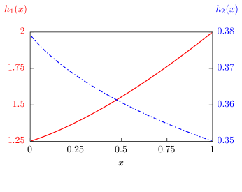
Figure 4: Plots of the functions $h_{1}(x)$ and $h_{2}(x)$ defined in Eq. (24). Note that both functions are positive and vary weakly in the interval $0<x<1$.

Both $h_{1}(x)$ and $h_{2}(x)$ are plotted in Fig. 4. We note that the changes in $h_{1}(x)$ and $h_{2}(x)$ in the range $0<x<1$ are relatively small, implying that our results should not depend significantly on the value of $\gamma_{z}/\gamma_{0}$. More importantly, both functions are positive for $0<x<1$, which implies that the overall coefficient of the cubic term is negative. For later convenience, we re-express Eq. (23) as:

$$\mathcal{F}_{\mathrm{EM}} [\psi]=$$ (25)

$$-\frac{\lambda_{0}}{3}|\psi|^{3}\left[1+\frac{\lambda_{3}}{\lambda_{0}}\left(\cos^{2}2\alpha+\sin^{2}2\alpha\cos^{2}\beta\right)\right]\mbox{,}$$

where the positive parameters $\lambda_{0}$ and $\lambda_{3}$ are defined as

$$\lambda_{0} \equiv\sqrt{32\pi}\left(\gamma_{0}q_{0}^{2}\mu_{0}\right)^{3/2}T\>h_{1}\left(\frac{\gamma_{z}}{\gamma_{0}}\right)\quad,$$ (26)

$$\lambda_{3} \equiv\left(\frac{\gamma_{3}}{\gamma_{0}}\right)^{2}\sqrt{32\pi}\left(\gamma_{0}q_{0}^{2}\mu_{0}\right)^{3/2}T\>h_{2}\left(\frac{\gamma_{z}}{\gamma_{0}}\right).$$

As we pointed out above, while such a negative non-analytic cubic term also appears in the $s$-wave case and in the isotropic $p$-wave case [35, 42], the novelty here is that the non-analytic contribution also depends on $\alpha$ and $\beta$ due to the in-plane anisotropy of the superconducting stiffness. From Eq. (25), since $\lambda_{3}>0$, it is clear that the term $\mathcal{F}_{\mathrm{EM}}[\psi]$ is minimized for $\beta=0$ and arbitrary $\alpha$, which corresponds to a nematic superconducting instability, in agreement with our numerical analysis.

II.2 Leading instability of the renormalized free-energy

Having derived an approximate analytical expression for $\mathcal{F}_{\mathrm{EM}}[\psi]$, we are now in position to minimize the full free energy $\mathcal{F}_{\mathrm{eff}}[\psi]$ given by Eq. (15) to find the leading instability immediately below the superconducting transition temperature. Using Eqs. (4) and (25), we obtain:

$$\mathcal{F}_{\mathrm{eff}}[\psi]=\frac{r}{2}|\psi|^{2}-\frac{\lambda_{0}}{3}|\psi|^{3}+\frac{u}{4}|\psi|^{4}$$ (27)

$$+\left(\frac{g}{4}|\psi|^{4}-\frac{\lambda_{3}}{3}|\psi|^{3}\right)\left(\cos^{2}2\alpha+\sin^{2}2\alpha\cos^{2}\beta\right).$$

The key point is that the leading superconducting instability of the system – chiral or nematic – is determined by the competition between the quartic and cubic terms, which share the same functional dependence on $\alpha$ and $\beta$. While the cubic term always favors the nematic phase, the quartic term may favor either the nematic or the chiral state depending on the sign of $g$, as shown in Fig. 2 above.

The presence of a negative cubic term renders the superconducting transition first-order. As a result, one has to compare the free energies of the two possible solutions – nematic ($\beta=0$) and chiral ($\beta=\pm\tfrac{\pi}{2}$, $\alpha=\tfrac{\pi}{4}$). Note that, because the functional dependence of the renormalized free-energy density $\mathcal{F}_{\mathrm{eff}}[\psi]$ on $\alpha$ and $\beta$ is the same as the dependence displayed by the bare free-energy density $\mathcal{F}_{0}[\psi]$, no additional solutions besides the chiral and nematic ones are expected to arise from the minimization of the free energy. In either case, after substituting the appropriate values for the angles, the free energy acquires the same general form:

$$\mathcal{F}_{\mathrm{eff}}^{(\mu)}[\psi]=\frac{r}{2}|\psi|^{2}-\frac{\lambda_{\mu}}{3}|\psi|^{3}+\frac{u_{\mu}}{4}|\psi|^{4}\mbox{,}$$ (28)

where $\mu$ denotes the nematic ($\mu=\mathrm{nem}$) or the chiral ($\mu=\mathrm{ch}$) solution. We have:

$$\begin{aligned} \lambda_{\mathrm{nem}}&=\lambda_{0}+\lambda_{3}\>;\\ \lambda_{\mathrm{ch}}&=\lambda_{0}\>;\end{aligned}\qquad\begin{aligned} u_{\mathrm{nem}}&=u+g\\ u_{\mathrm{ch}}&=u\end{aligned}$$ (29)

It is straightforward to minimize Eq. (28) with respect to $\left|\psi\right|$ and find the condition on the reduced temperature $r$ for which the minimized free energy becomes smaller than that of the non-superconducting phase. We find that the first-order transition for the $\mu$ solution takes place at the reduced temperature $r=r_{\mu}$ given by:

$$r_{\mu}=\frac{2\lambda_{\mu}^{2}}{9u_{\mu}}.$$ (30)

At this transition, the superconducting order parameter jumps according to:

$$\Delta|\psi|_{\mu}=\frac{2\lambda_{\mu}}{3u_{\mu}}$$ (31)

Therefore, the leading (first-order) superconducting instability is that whose free energy becomes negative first, i.e. the solution with the largest $r_{\mu}$ value. Using Eqs. (29) and (30), the phase boundary $g^{*}(u)$ between the chiral and nematic phases in the $(u,g)$ parameter-space is given implicitly by the condition $r_{\mathrm{ch}}=r_{\mathrm{nem}}$, from which we derive:

$$g^{*}(u)=\left[\left(1+\frac{\lambda_{3}}{\lambda_{0}}\right)^{2}-1\right]u.$$ (32)

Note that the chiral solution is the leading instability for $g>g^{*}$ whereas the nematic solution is the leading one for $g<g^{*}$.

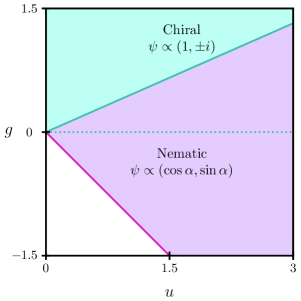
Figure 5: Phase diagram, in the $(u,g)$ parameter-space, of the leading superconducting instability obtained by minimizing the effective free energy in Eq. (27), which is renormalized by the electromagnetic field fluctuations. The dotted line represents the phase boundary of the bare free energy, see Fig. 2. The phase boundary separating the nematic and chiral solutions is a straight line given by Eq. (32). For this plot, we set $\tfrac{\lambda_{3}}{\lambda_{0}}=0.2$.

The phase diagram of the renormalized free-energy is shown in Fig. 5. Compared with the mean-field phase diagram of the bare free-energy in Fig. 2, the main difference is that the nematic solution becomes the leading instability in a region of the parameter-space where $g>0$, thus displacing the chiral solution. Indeed, because $\lambda_{3},\,\lambda_{0}>0$, it follows that $g^{*}>0$. This implies that the nematic-chiral phase boundary of the renormalized free-energy moves to the region of the parameter-space where the chiral solution used to be the leading instability. As a result, the nematic solution is favored over a wider range of parameters as compared to the bare free-energy case.

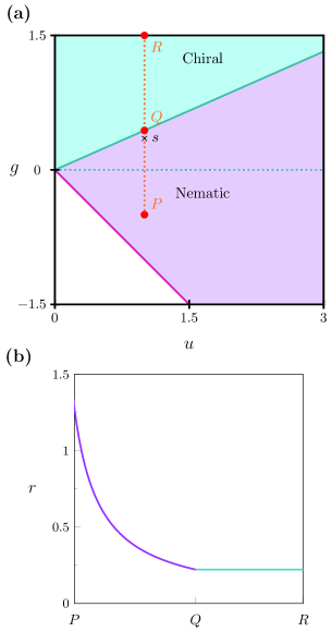
Figure 6: (a) Definition of the path $P\rightarrow Q\rightarrow R$ in the phase diagram of Fig. 5. (b) Evolution of the reduced temperature $r$ where either the nematic (purple line) or the chiral (cyan line) transition takes place, i.e. $\mathrm{max}\left(r_{\mathrm{nem}},\,r_{\mathrm{ch}}\right)$, along the path $P\rightarrow Q\rightarrow R$. For these plots, we used $\lambda_{0}=1$ and $\lambda_{3}=0.2$. We also set $u=1$ along the path $P\rightarrow Q\rightarrow R$.

Another difference between the phase diagrams of Figs. 2 (bare free-energy) and 5 (free-energy renormalized by electromagnetic fluctuations) is that, in the former, the leading instability is second-order and occurs always at the reduced temperature $r=0$. In the latter, the transition is first-order and occurs for a positive $r_{\mu}$ given by Eq. (30), which changes across the phase diagram. This is illustrated in Fig. 6(b), where we plot $\mathrm{max}\left(r_{\mathrm{nem}},\,r_{\mathrm{ch}}\right)$ along the $P-Q-R$ path shown in Fig. 6(a).

Based on the quantitative estimates of Ref. [35], one generally expects the cubic coefficients $\lambda_{0}$ and $\lambda_{3}$ to be small, rendering the first-order transition very weak – in other words, one expects the jump $\Delta\left|\psi\right|_{\mu}$ in Eq. (31) to be very small, $\lambda_{i}\ll u$. It is important to note, however, that this does not imply that the effect of the electromagnetic field fluctuations on the selection between the chiral and the nematic phase is negligible. Instead, from the condition (32), we conclude that this effect is significant when the ratio between the quartic coefficients $g/u$ is comparable to the ratio between the cubic coefficients $\lambda_{3}/\lambda_{0}$. As a result, even though $\lambda_{i}\ll u$, this does not preclude $g/u\sim\lambda_{3}/\lambda_{0}$.

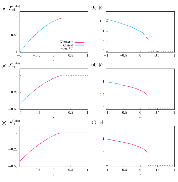
Figure 7: (a) and (b): Evolution of the free energy minimum and of the magnitude of the order parameter, as functions of the reduced temperature $r$. Both plots correspond to the point $s$ in the phase diagram of Fig. 6(a). This means that we set $u=1$, $g=0.35$, $\lambda_{0}=1$ and $\lambda_{3}=0.2$. (c)-(f): Same as (a)-(b) but in these cases, the sixth-order terms in Eq. (33) are included. We set $v_{1}=1$, $v_{2}=0$ and either $v_{3}=0.10$ [panels(c) and (d)] or $v_{3}=0.15$ [panels (e) and (f)].

Going back to the effective free-energy in Eq. (27), it is interesting to analyze in more depth the interplay between the cubic and quartic terms. Naively, one might have expected that the nematic instability should always be the leading one, since the cubic term favors the nematic phase, whereas the chiral phase is only favored by the higher-order quartic term (for $g>0$, of course). The reason why the quartic term can outcompete the cubic one is because of the first-order character of the transition. This can be seen by noting that, immediately below the first-order transition, the combination $\tilde{g}\equiv\left(\frac{g}{4}-\frac{\lambda_{3}}{3\Delta|\psi|}\right)$ acts as an effective coefficient of the angular-dependent term in Eq. (27), where $\Delta|\psi|$ is the jump in the superconducting order parameter. Plugging in the value for $\Delta|\psi|_{\mathrm{ch}}$ obtained from Eq. (31), we find that $\tilde{g}>0$ in the regime $g>g^{*}$. Clearly, a positive $\tilde{g}$ favors $\beta=\pm\pi/2$ and $\alpha=\pi/4$, consistent with a chiral phase. Conversely, substituting the value for $\Delta|\psi|_{\mathrm{nem}}$, we find that $\tilde{g}<0$ in the regime $g<g^{*}$. A negative effective coefficient $\tilde{g}$ favors $\beta=0$, consistent with a nematic phase.

That the nematic phase can be stabilized in a regime where the bare parameters of the free-energy would predict a chiral phase is the main result of our paper. Thus, electromagnetic field fluctuations tilt the balance between the chiral and nematic states in favor of the latter. Formally, this effect is enabled by the finite stiffness coefficient $\gamma_{3}$ in Eq. (6). Indeed, $\gamma_{3}=0$ gives $\lambda_{3}=0$, which in turn implies $g^{*}(u)=0$, recovering the nematic-chiral phase boundary obtained from the bare free-energy. Note that, as long as the gradient coefficients $K_{1}$ and $K_{2}$ in Eq. (5) are different, $\gamma_{3}$ will be nonzero. Therefore, the microscopic origin of this effect is the fact that the stiffness of a two-component superconductor is not isotropic in momentum space.

II.3 Stability of the superconducting nematic state below $T_{c}$

The phase diagram obtained in Fig. 5 refers to the leading instability immediately below the first-order transition temperature $T_{c}$ set by $r_{\mathrm{nem}}$ or $r_{\mathrm{ch}}$. In this section, we investigate the stability of the nematic solution below the superconducting transition in the region $0<g<g^{*}$. Of course, since we are employing a Ginzburg-Landau approach, this analysis is only formally valid near $r_{\mathrm{nem}}$. As such, our calculations cannot be used to establish what the zero-temperature superconducting ground state is.

To assess the nematic phase below $r_{\mathrm{nem}}$, it is important to also include the sixth-order terms of the Landau free-energy $\mathcal{F}_{0}\left[\psi\right]$ that we have neglected so far. This is because, as discussed above, minimization of the quartic-order free-energy does not fix the value of the angle $\alpha$ that characterizes the relative amplitude of the two components of the gap function in the nematic superconducting state, $\psi_{\mathrm{nem}}\propto(\cos{\alpha},\sin{\alpha})$. A sixth-order term lowers this artificial $U(1)$ symmetry to a $Z_{3}$ symmetry, as expected for a lattice with threefold rotational symmetry [44, 23]. We thus include in our analysis the three sixth-order terms that are allowed by the threefold rotational symmetry of the lattice [21]:

$$\bar{\mathcal{F}}_{0}\left[\psi\right]= \frac{v_{1}}{6}|\psi|^{6}+\frac{v_{2}}{6}|\psi|^{2}\left[|\psi|^{4}-\left(\bar{\psi}\tau_{2}\psi\right)^{2}\right]$$ (33)

$$+\frac{v_{3}}{6}\left(\bar{\psi}\tau_{3}\psi\right)\left[\left(\bar{\psi}\tau_{3}\psi\right)^{2}-3\left(\bar{\psi}\tau_{1}\psi\right)^{2}\right]\mbox{,}$$

where new Landau coefficients $v_{1}$, $v_{2}$ and $v_{3}$ were introduced. To ensure that the free energy remains bounded, they must satisfy $v_{1}>0$, $v_{1}+v_{2}>0$ and $v_{1}+v_{2}-|v_{3}|>0$. The first sixth-order term above, with coefficient $v_{1}$, does not distinguish between the chiral and the nematic states. The second sixth-order term, with coefficient $v_{2}$, can be rewritten in terms of the angles $\alpha$ and $\beta$ as:

$$\bar{\mathcal{F}}_{0}^{(2)}\left[\psi\right]=\frac{v_{2}}{6}|\psi|^{6}\left(1-\sin^{2}2\alpha\,\sin^{2}\beta\right).$$ (34)

Thus, if $v_{2}>0$, the chiral state is favored by this term, whereas if $v_{2}<0$, the nematic state is favored. As for the third sixth-order term, with coefficient $v_{3}$, it can be rewritten as:

$$\bar{\mathcal{F}}_{0}^{(3)}\left[\psi\right]=\frac{v_{3}}{6}|\psi|^{6}\cos 2\alpha\left(\cos^{2}2\alpha-3\sin^{2}2\alpha\,\cos^{2}\beta\right).$$ (35)

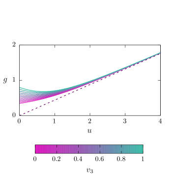
Figure 8: Nematic-chiral phase boundary in the $(u,g)$ parameter-space. The dashed line is the phase boundary in the absence of the sixth-order terms, as shown in Fig. 5. Each solid curve represents the phase boundary for different values of $v_{3}$, as shown by the color-scale bar. In all cases, we set $\tfrac{\lambda_{3}}{\lambda_{0}}=0.2$, $v_{1}=1$, and $v_{2}=0$.

This term not only favors the nematic phase ($\beta=0$), regardless of the sign of $v_{3}$, but it also restricts the allowed values of $\alpha$ to a discrete set of six values. Indeed, setting $\beta=0$, we obtain $\bar{\mathcal{F}}_{0}^{(3)}\left[\psi\right]=\tfrac{v_{3}}{6}|\psi|^{6}\cos 6\alpha$. As a result, if $v_{3}>0$, this term is minimized by $\alpha=\tfrac{\left(2n+1\right)\pi}{6}$ with $n=0,1,...,5$; conversely, if $v_{3}<0$, minimization gives $\alpha=\tfrac{2n\pi}{6}$ with $n=0,1,...,5$.

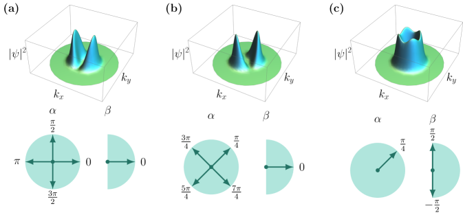
Figure 9: Absolute value squared of the gap function along a circular Fermi surface for a $(p_{x},\,p_{y})$-wave superconductor on a tetragonal lattice. Three ground states are possible. A similar analysis was shown previously in Ref. [22]. (a) The $\mathrm{B_{1g}}$ nematic superconducting state, which reduces the $C_{4z}$ rotational symmetry of the lattice to a $C_{2z}$ symmetry. In this plot, we set $\alpha=0$. (b) The $\mathrm{B_{2g}}$ nematic superconducting state breaks the $C_{4z}$ rotational symmetry of the lattice as well; in this plot, we used $\alpha=\tfrac{\pi}{4}$. (c) The chiral superconducting state is characterized by $\alpha=\tfrac{\pi}{4}$ and $\beta=\pm\tfrac{\pi}{2}$. It does not break any lattice symmetry, but it breaks time reversal symmetry.

To investigate the stability of the nematic phase below the superconducting transition, we numerically minimize the full free-energy $\bar{\mathcal{F}}_{\mathrm{eff}}\equiv\mathcal{F}_{\mathrm{eff}}+\bar{\mathcal{F}}_{0}$, as given by Eqs. (27) and (33), in both the nematic and chiral channels for $r<r_{\mathrm{nem}}$. Our interest is in the region $0<g<g^{*}$, where the electromagnetic field fluctuations change the leading instability from chiral to nematic. For concreteness, we consider the point $s$ in the phase diagram of Fig. 6(a), which is close to the nematic-chiral phase boundary. The evolution of the free energy minimum, $\mathcal{\bar{F}}_{\mathrm{eff}}^{\mathrm{(min)}}$, as function of $r$ is shown in Fig. 7 (left panels), accompanied by the evolution of the absolute value of the superconducting order parameter $\left|\psi\right|$ (right panels). Without the sixth-order terms [panels (a)-(b)], the nematic state undergoes a first-order transition to the chiral state relatively close to $r_{\mathrm{nem}}$.

However, upon inclusion of the sixth-order contributions – particularly the $\bar{\mathcal{F}}_{0}^{(3)}\left[\psi\right]$ term that is responsible for enforcing the discreteness of the $\alpha$ values – we find that the nematic solution remains the global energy minimum over a significantly wider range of reduced temperatures $r$ [panels (c)-(f)]. Interestingly, this effect is apparent even for $\left|v_{3}\right|\ll v_{1}$. A finite $v_{2}$ can either extend the nematic solution to an even larger range of reduced temperatures, if $v_{2}<0$, or compress it to a narrower range, if $v_{2}>0$. Therefore, we conclude that the sixth-order term (35) is important not only to lift the accidental $U(1)$ symmetry of $\alpha$, but also to stabilize the nematic phase promoted by the electromagnetic field fluctuations below the superconducting transition.

Another effect caused by the the sixth-order terms is a change in the nematic-chiral phase boundary of Fig. 5. As shown in Fig. 8, upon increasing the coefficient $v_{3}$ (while keeping $v_{1}$ and $v_{2}$ fixed), the phase boundary acquires a curvature and is no longer linear. Importantly, this effect is only significant close to the origin of the $(u,g)$ parameter-space. As one moves away from the origin, all the boundaries become asymptotically close to the linear boundary whose slope is determined solely by the cubic coefficients $\lambda_{0}$ and $\lambda_{3}$.

III Two-component superconductor on the tetragonal lattice

The main result derived in Sec. II – that electromagnetic gauge-field fluctuations favor a nematic over a chiral superconducting state – is not unique to the triangular lattice. In this section, we extend the analysis to the case of a two-component superconductor on a tetragonal lattice. For concreteness, we consider the point group $D_{4h}$, such that $\psi=\left(\psi_{1},\,\psi_{2}\right)$ can transform as either the $E_{g}$ irrep – which corresponds to a $(d_{xz},\,d_{yz})$-wave superconductor – or the $E_{u}$ irrep – corresponding to a $(p_{x},\,p_{y})$-wave superconductor. To start, we review the known results for the mean-field phase diagram (which can be found e.g. in Refs. [21, 49]), following the notation of Ref. [22]. The superconducting order parameter can still be parametrized as in Eq. (1). However, instead of two, there are three possible superconducting ground states: the $\mathrm{B_{1g}}$ nematic state $\psi=\left(1,\,0\right)/(0,1)$, corresponding to $\alpha=\tfrac{2n\pi}{4}$ and $\beta=0$, with $n=0,...,3$; the $\mathrm{B_{2g}}$ nematic state $\psi=\left(1,\,\pm 1\right)$, corresponding to $\alpha=\tfrac{(2n+1)\pi}{4}$ and $\beta=0$, with $n=0,...,3$; and the chiral state $\psi=\left(1,\,\pm i\right)$, corresponding to $\alpha=\tfrac{\pi}{4}$, and $\beta=\pm\tfrac{\pi}{2}$. The corresponding absolute values of the gap function are shown in Fig. 9 for the particular case of a $(p_{x},\,p_{y})$-wave state – see also Ref. [22], where a similar analysis was presented. Both $\mathrm{B_{1g}}$ and $\mathrm{B_{2g}}$ nematic superconducting states break the fourfold ($C_{4z}$) rotational symmetry of the system, lowering it to twofold ($C_{2z}$). However, they are not symmetry-equivalent, as the $\mathrm{B_{1g}}$ state preserves the $\sigma_{v}$ mirror reflections, whereas the $\mathrm{B_{2g}}$ state preserves the $\sigma_{d}$ mirror reflections.

To proceed, we write the full Ginzburg-Landau free-energy density as in Eq. (2). The non-gradient terms are given by [21, 49]:

$$\begin{aligned} \mathcal{F}_{0}[\psi]\end{aligned} =\frac{r}{2}|\psi|^{2}+\frac{u}{4}|\psi|^{4}+\frac{g}{4}\left(\bar{\psi}\tau_{3}\psi\right)^{2}+\frac{w}{4}\left(\bar{\psi}\tau_{1}\psi\right)^{2}$$ (36)

$$=\frac{r}{2}|\psi|^{2}+\frac{u}{4}|\psi|^{4}$$

$$+\frac{g}{4}|\psi|^{4}\cos^{2}2\alpha+\frac{w}{4}|\psi|^{4}\sin^{2}2\alpha\cos^{2}\beta.$$

In order for $\mathcal{F}_{0}[\psi]$ to be bounded, the Landau parameters must satisfy the conditions $u>0$, $w+u>0$ and $g+u>0$. Minimization of the free energy leads to the three possible superconducting solutions mentioned above. As shown in the mean-field phase diagram of Fig. 10, when $g<\min\left\{0,w\right\}$, the leading instability below $r<0$ is the $\mathrm{B_{1g}}$ nematic superconducting state. When $g>w$ and $w<0$, the selected state is the $\mathrm{B_{2g}}$ nematic, whereas for $g>0$ and $w>0$, it is the chiral state.

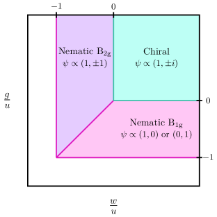
Figure 10: Mean-field phase diagram in the $\left(\frac{w}{u},\,\frac{g}{u}\right)$ parameter-space for a two-component superconductor on a tetragonal lattice, obtained by minimizing the free-energy in Eq. (36). The white area in this plot corresponds to the parameter-space region where the free-energy is unbounded from below.

The gradient terms are given by [21]:

$$\qquad\mathcal{F}_{\mathrm{grad}}[\psi]=K_{1}\!\left[\left|D_{x}\psi_{1}\right|^{2}\!+\!\left|D_{y}\psi_{2}\right|^{2}\right]$$ (37)

$$+\!K_{2}\!\left[\left|D_{x}\psi_{2}\right|^{2}\!+\!\left|D_{y}\psi_{1}\right|^{2}\right]\!+\!K_{3}\!\left[\left(D_{x}\psi_{1}\right)^{\ast}\left(D_{y}\psi_{2}\right)\!+\!c.c.\right]$$

$$+\!K_{4}\!\left[\left(D_{x}\psi_{2}\right)^{\ast}\left(D_{y}\psi_{1}\right)\!+\!c.c.\right]\!+\!K_{5}\!\left[\left|D_{z}\psi_{1}\right|^{2}\!+\!\left|D_{z}\psi_{2}\right|^{2}\right]\mbox{,}$$

where, as in Sec. II, $D_{x}=\partial_{x}-iq_{0}A_{x}$, etc. are the covariant derivatives and $K_{i}$ are the stiffness coefficients. Assuming that the order parameter is spatially uniform in the regime where the gauge-field fluctuations are strong, the equation above is simplified to:

$$\mathcal{F}_{\mathrm{grad}}[\psi]= q_{0}^{2}\gamma_{0}\left|\psi\right|^{2}\left(A_{x}^{2}+A_{y}^{2}\right)+q_{0}^{2}\gamma_{3}(\bar{\psi}\tau_{3}\psi)\left(A_{x}^{2}-A_{y}^{2}\right)$$ (38)

$$+2A_{x}A_{y}q_{0}^{2}\gamma_{1}(\bar{\psi}\tau_{1}\psi)+A_{z}^{2}q_{0}^{2}\gamma_{z}\left|\psi\right|^{2}\mbox{,}$$

where we have defined the effective stiffness coefficients as $\gamma_{z}=K_{5}$,

$$\gamma_{1} =\frac{K_{3}+K_{4}}{2},\!\quad\gamma_{3}=\frac{K_{1}-K_{2}}{2}\quad\!\mbox{and}\!\quad\gamma_{0}=\frac{K_{1}+K_{2}}{2}.$$ (39)

Note that, as compared to the triangular-lattice case, there is an additional stiffness coefficient in the case of the tetragonal lattice, since $\gamma_{1}\neq\gamma_{3}$. If these two coefficients were fine-tuned to acquire the same value, one would recover the results for the triangular lattice.

We now repeat the same steps as in Sec. II to integrate out the electromagnetic field fluctuations and obtain the effective free-energy density

$$\mathcal{F}_{\mathrm{eff}}\left[\psi\right] =\mathcal{F}_{0}\left[\psi\right]+\mathcal{F}_{\mathrm{EM}}[\psi]\mbox{,}$$ (40)

with $\mathcal{F}_{\mathrm{0}}[\psi]$ defined in Eq. (36). The term $\mathcal{F}_{\mathrm{EM}}[\psi]$, resulting from the gauge-field fluctuations, acquires the same form as in Eq. (20), with $a_{\pm}^{2}$ still defined by Eq. (18), but with the new dimensionless quantities $b$ and $c$ given by:

$$\!b=\!\frac{\gamma_{z}}{\gamma_{0}}+1+\left(1-\frac{\gamma_{z}}{\gamma_{0}}\right)x^{2}$$ (41)

$$-\!\left(1\!-\!x^{2}\right)\!\left(\frac{\gamma_{3}}{\gamma_{0}}\cos 2\alpha\cos 2\phi+\!\frac{\gamma_{1}}{\gamma_{0}}\cos\beta\sin 2\alpha\sin 2\phi\right)$$

and

$$\!c=\!\frac{\gamma_{z}}{\gamma_{0}}\!+\!\!\left[1\!-\!\frac{\gamma_{z}}{\gamma_{0}}\!-\!\left(\frac{\gamma_{3}}{\gamma_{0}}\cos 2\alpha\right)^{2}\!\!-\!\left(\frac{\gamma_{1}}{\gamma_{0}}\cos\beta\sin 2\alpha\right)^{2}\right]\!x^{2}\!$$ (42)

$$-\frac{\gamma_{z}}{\gamma_{0}}\!\left(1\!-\!x^{2}\right)\!\left(\frac{\gamma_{3}}{\gamma_{0}}\cos 2\alpha\cos 2\phi+\frac{\gamma_{1}}{\gamma_{0}}\cos\beta\sin 2\alpha\sin 2\phi\right).$$

We first study numerically the dependence of the cubic term $\mathcal{F}_{\mathrm{EM}}[\psi]$ on $\alpha$ and $\beta$. As in the preceding section, it is convenient to express it in terms of the dimensionless integral $f^{(3)}$ given by Eq. (22), such that:

$$\mathcal{F}_{\mathrm{EM}}[\psi]=\frac{T\psi_{s}^{3}}{12\pi}\,f^{(3)}\left(\frac{\gamma_{1}}{\gamma_{0}},\frac{\gamma_{3}}{\gamma_{0}},\frac{\gamma_{z}}{\gamma_{0}},\alpha,\beta\right)\mbox{.}$$ (43)

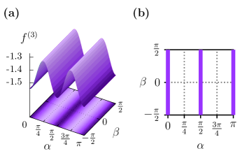
Figure 11: (a) Dimensionless coefficient of the cubic term $f^{(3)}\left(\alpha,\beta\right)$ as a function of $\alpha$ and $\beta$ for fixed $\tfrac{\gamma_{1}}{\gamma_{0}}=0$, $\tfrac{\gamma_{3}}{\gamma_{0}}=0.8$ and $\tfrac{\gamma_{z}}{\gamma_{0}}=0.1$. (b) Location of the minima of $f^{(3)}\left(\alpha,\beta\right)$ on the $(\alpha,\beta)$ plane. The minima correspond to the $\mathrm{B_{1g}}$ nematic superconducting state with order parameter $\psi\propto(1,0)$ or $\psi\propto(0,1)$.

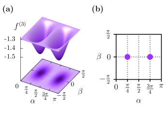
Figure 12: (a) Dimensionless coefficient of the cubic term $f^{(3)}\left(\alpha,\beta\right)$ as a function of $\alpha$ and $\beta$ for fixed $\tfrac{\gamma_{1}}{\gamma_{0}}=0.8$, $\tfrac{\gamma_{3}}{\gamma_{0}}=0$ and $\tfrac{\gamma_{z}}{\gamma_{0}}=0.1$. (b) Location of the minima of $f^{(3)}\left(\alpha,\beta\right)$ on the $(\alpha,\beta)$ plane. The minima correspond to the $\mathrm{B_{2g}}$ nematic superconducting state with order parameter $\psi\propto(1,\pm 1)$.

We systematically analyzed $f^{(3)}\left(\alpha,\beta\right)$ numerically for various values of the stiffness coefficients. Because $f^{(3)}$ only depends on $\cos 2\alpha$ and $\sin 2\alpha$, we restricted the range of $\alpha$ values to $[0,\pi]$. The stiffness coefficients were varied systematically in the ranges $\tfrac{\gamma_{z}}{\gamma_{0}}\in[0,1]$, $\tfrac{\gamma_{1}}{\gamma_{0}}\in[-1,1]$, and $\tfrac{\gamma_{3}}{\gamma_{0}}\in[-1,1]$. In all cases, we found $f^{(3)}\left(\alpha,\beta\right)<0$. More importantly, the values of $\alpha$ and $\beta$ that minimize $f^{(3)}\left(\alpha,\beta\right)$ were found to always correspond to one of the two nematic superconducting states. In particular, in the cases where $|\gamma_{1}|<|\gamma_{3}|$, the minima are located at $\alpha=2n\pi/4$ with integer $n$, corresponding to the $\mathrm{B_{1g}}$ nematic superconducting state $\psi\propto(1,0)/(0,1)$. This is illustrated in Fig. 11, where we show $f^{(3)}\left(\alpha,\beta\right)$ for the particular case $\tfrac{\gamma_{1}}{\gamma_{0}}=0$, $\tfrac{\gamma_{3}}{\gamma_{0}}=0.8$, and $\tfrac{\gamma_{z}}{\gamma_{0}}=0.1$. Conversely, in all the cases where $|\gamma_{1}|>|\gamma_{3}|$, the minima are at $\beta=0$ and $\alpha=\left(2n+1\right)\pi/4$ with integer $n$, corresponding to the $\mathrm{B_{2g}}$ nematic superconducting state $\psi\propto(1,\pm 1)$. Such a behavior is illustrated in Fig. 12 for the particular case $\tfrac{\gamma_{1}}{\gamma_{0}}=0.8$, $\tfrac{\gamma_{3}}{\gamma_{0}}=0$, and $\tfrac{\gamma_{z}}{\gamma_{0}}=0.1$.

Following the same steps as in Sec. II, we perform an analytical expansion of $f^{(3)}\left(\frac{\gamma_{1}}{\gamma_{0}},\frac{\gamma_{3}}{\gamma_{0}},\frac{\gamma_{z}}{\gamma_{0}},\alpha,\beta\right)$ to second order in $\gamma_{1}/\gamma_{0}$ and $\gamma_{3}/\gamma_{0}$. We obtain:

$$\mathcal{F}_{\mathrm{EM}}[\psi]\sim-\frac{T\psi_{s}^{3}}{12\pi}\left\{h_{1}\left(\frac{\gamma_{z}}{\gamma_{0}}\right)+\right.$$ (44)

$$\left.h_{2}\left(\frac{\gamma_{z}}{\gamma_{0}}\right)\left[\left(\frac{\gamma_{1}}{\gamma_{0}}\sin 2\alpha\cos\beta\right)^{2}+\left(\frac{\gamma_{3}}{\gamma_{0}}\cos 2\alpha\right)^{2}\right]\right\}\mbox{,}$$

where $h_{1}(x)$ and $h_{2}(x)$ were previously defined in Eq. (24) and plotted in Fig. 4. Minimization of $\mathcal{F}_{\mathrm{EM}}[\psi]$ leads to $\alpha=\left(2n+1\right)\pi/4$ and $\beta=0$ when $\left|\gamma_{1}\right|>\left|\gamma_{3}\right|$ and to $\alpha=2n\pi/4$ when $\left|\gamma_{3}\right|>\left|\gamma_{1}\right|$, in agreement with the numerical analysis. For convenience, we define the coefficients:

$$\lambda_{0} \equiv\sqrt{32\pi}\left(\gamma_{0}q_{0}^{2}\mu_{0}\right)^{3/2}T\>h_{1}\left(\frac{\gamma_{z}}{\gamma_{0}}\right)\,,$$ (45)

$$\lambda_{1} \equiv\sqrt{32\pi}\left(\gamma_{0}q_{0}^{2}\mu_{0}\right)^{3/2}T\>\left(\frac{\gamma_{1}}{\gamma_{0}}\right)^{2}h_{2}\left(\frac{\gamma_{z}}{\gamma_{0}}\right)\mbox{,}$$

$$\lambda_{3} \equiv\lambda_{1}\left(\frac{\gamma_{3}}{\gamma_{1}}\right)^{2},$$

and rewrite the cubic term as:

$$\mathcal{F}_{\mathrm{EM}} [\psi]=$$ (46)

$$-\frac{\lambda_{0}}{3}|\psi|^{3}\left(1+\frac{\lambda_{1}}{\lambda_{0}}\sin^{2}2\alpha\cos^{2}\beta+\frac{\lambda_{3}}{\lambda_{0}}\cos^{2}2\alpha\right)\mbox{,}$$

Since $\mathcal{F}_{\mathrm{EM}}[\psi]$ has the same functional dependence on $\alpha$ and $\beta$ as the bare free-energy density $\begin{aligned} \mathcal{F}_{0}[\psi]\end{aligned}$, minimization of the total free-energy density $\mathcal{F}_{\mathrm{eff}}\left[\psi\right]$ should yield the same solutions as $\begin{aligned} \mathcal{F}_{0}[\psi]\end{aligned}$. Like we did in Sec. II, to find the leading instability, we compare the free energies of the three solutions, since the cubic term renders the transition first-order. In all cases, after substituting the values for $\alpha$ and $\beta$ corresponding to each solution, the free-energy density acquires the same form:

$$\mathcal{F}_{\mathrm{eff}}^{(\mu)}[\psi]=\frac{r}{2}|\psi|^{2}-\frac{\lambda_{\mu}}{3}|\psi|^{3}+\frac{u_{\mu}}{4}|\psi|^{4}$$ (47)

where $\mu$ labels the type of solution ($\mu=\mathrm{B_{1g}},\>\mathrm{B_{2g}},\>\mathrm{ch}$) and:

$$\begin{aligned} \lambda_{\mathrm{B_{1g}}}&=\lambda_{0}+\lambda_{3}\>;\\ \lambda_{\mathrm{B_{2g}}}&=\lambda_{0}+\lambda_{1}\>;\\ \lambda_{\mathrm{ch}}&=\lambda_{0}\>;\end{aligned}\qquad\begin{aligned} u_{\mathrm{B_{1g}}}&=u+g\\ u_{\mathrm{B_{2g}}}&=u+w\\ u_{\mathrm{ch}}&=u\end{aligned}$$ (48)

As we showed in Sec. II, the first-order transition associated with the free-energy in Eq. (47) takes place at the reduced temperature $r_{\mu}=\frac{2\lambda_{\mu}^{2}}{9u_{\mu}}$. Thus, the leading instability is the one with the largest transition temperature:

$$r_{\mathrm{B_{1g}}} =\frac{2\left(\lambda_{0}+\lambda_{3}\right)^{2}}{9\left(u+g\right)}$$

$$r_{\mathrm{B_{2g}}} =\frac{2\left(\lambda_{0}+\lambda_{1}\right)^{2}}{9\left(u+w\right)}$$

$$r_{\mathrm{ch}} =\frac{2\lambda_{0}^{2}}{9u}$$ (49)

It is now straightforward to determine the phase boundaries in the $\left(\frac{w}{u},\,\frac{g}{u}\right)$ parameter-space. The chiral solution is the leading instability in the region bounded by $w>w^{*}$ and $g>g^{*}$, where:

$$\frac{w^{\ast}}{u} =\left[\left(\frac{\lambda_{1}}{\lambda_{0}}+1\right)^{2}-1\right]$$

$$\frac{g^{\ast}}{u} =\left[\left(\frac{\lambda_{3}}{\lambda_{0}}+1\right)^{2}-1\right]\>.$$ (50)

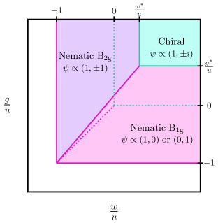
Figure 13: Phase diagram, in the $\left(\frac{w}{u},\,\frac{g}{u}\right)$ parameter-space, for a two-component superconductor on a tetragonal lattice obtained from minimization of the free-energy renormalized by electromagnetic field fluctuations. The dotted lines represent the phase boundaries of the mean-field phase diagram (see Fig. 10). For this plot, we set $\tfrac{\lambda_{1}}{\lambda_{0}}=0.2$ and $\tfrac{\lambda_{3}}{\lambda_{0}}=0.3$. The quantities $w^{\ast}$ and $g^{\ast}$ are defined in Eq. (50), and in this plot are given by $w^{\ast}=0.44u$ and $g^{\ast}=0.69u$.

The fact that $w^{\ast},g^{\ast}>0$ implies that the region of the phase diagram where the chiral solution is realized shrinks with respect to the region occupied by the chiral solution in the mean-field phase diagram. This is illustrated in Fig. 13, where the renormalized phase boundaries are shown by the solid lines whereas the bare phase boundaries are given by the dashed lines. Therefore, after renormalization by the electromagnetic field fluctuations, the nematic state becomes the leading superconducting instability over a significant range of parameters for which the mean-field analysis would predict a chiral state. This result is analogous to the case of the two-component superconductor on the triangular lattice.

There is, however, one important difference, as there are two symmetry-distinct nematic superconducting states on the tetragonal lattice, namely the $\mathrm{B_{1g}}$ and $\mathrm{B_{2g}}$ nematic solutions. Comparing $r_{\mathrm{B_{1g}}}$ and $r_{\mathrm{B_{2g}}}$, we find that, for $w<w^{*}$ and $g<g^{*}$, the phase boundary $\tilde{g}\left(w\right)$ separating the two nematic phases is given by:

$$\frac{\tilde{g}\left(w\right)}{u}=-1+\left(\frac{w}{u}+1\right)\left(\frac{\lambda_{3}+\lambda_{0}}{\lambda_{1}+\lambda_{0}}\right)^{2}\>,$$ (51)

such that the $\mathrm{B_{1g}}$ state is realized for $g<\tilde{g}\left(w\right)$ and the $\mathrm{B_{2g}}$ state, for $g>\tilde{g}\left(w\right)$. Compared to the phase boundary of the mean-field phase diagram, $\tilde{g}_{\mathrm{MF}}\left(w\right)=w$, we conclude that, for $\lambda_{3}>\lambda_{1}$, the $\mathrm{B_{1g}}$ nematic solution occupies a region of the parameter-space that was occupied by the $\mathrm{B_{2g}}$ nematic solution in the mean-field case. This case is illustrated in Fig. 13. Conversely, for $\lambda_{1}>\lambda_{3}$, it is the $\mathrm{B_{2g}}$ solution that occupies an expanded region of the parameter-space.

IV Conclusions

In this paper, we showed that electromagnetic fluctuations play an important role in the selection between nematic versus chiral superconductivity for two-component superconductors, such as $\left(p_{x},p_{y}\right)$-wave and $\left(d_{x^{2}-y^{2}},d_{xy}\right)$-wave states. Upon integrating out these gauge-field fluctuations, they generate non-analytic cubic terms in the free-energy that induce a first-order transition, similarly to the cases of the $s$-wave and multi-component superconductors with isotropic stiffness analyzed elsewhere [35, 41, 42], as well as of color superconductivity involving quarks and gluons [43]. The crucial difference is that, for the two-component superconductors studied here, the superconducting stiffness – or, equivalently, the correlation length – is not isotropic in the $(x,y)$ plane due to the crystalline lattice. This makes the non-analytic term in the free-energy sensitive to whether the superconducting state is nematic or chiral, favoring the former over the latter. The relevance of this result stems from the fact that weak-coupling microscopic calculations generally place the system in a region of the parameter-space where minimization of the mean-field free-energy predicts a chiral state. However, as shown here, the non-analytic free-energy term arising from the gauge-field fluctuations changes the nature of the leading instability in a significant portion of this parameter-space region from chiral to nematic. As a result, the effect of the electromagnetic field fluctuations on the superconducting free-energy provides a mechanism by which a nematic state can be stabilized over the chiral one, without requiring fine tuning or coupling to non-superconducting degrees of freedom.

We emphasize that the size of the effect uncovered here is not necessarily small, even if the induced transition is very weakly first-order, as is the case for $s$-wave superconductors. Indeed, a weak first-order transition generally implies that the coefficients of the cubic terms ($\lambda_{0}$ and $\lambda_{3}$ in our notation for the triangular-lattice case) are much smaller than the coefficients of the quartic terms ($u$ and $g$ in our notation). However, the change in the leading superconducting instability from chiral to nematic promoted by the gauge-field fluctuations takes place when $g/u\lesssim\lambda_{3}/\lambda_{0}$, i.e. it depends on how the ratio between the quartic terms compares with the ratio between the cubic terms. Importantly, both ratios may be comparable even if $\lambda_{0},\lambda_{3}\ll u,g$. This analysis reveals that the role of the electromagnetic fluctuations on multi-component superconductors is potentially much more significant than in the case of single-component superconductors.

It is important to discuss the limitations of our approach. In order to integrate out the electromagnetic field fluctuations, we assumed that, in the temperature range where these fluctuations are significant, the spatial variation of the superconducting order parameter can be neglected. Formally, this can only be justified in type-I superconductors, for which the correlation length is smaller than the coherence length [35]. Other methods that do not require this approximation of a uniform superconducting order parameter were also employed for the cases of the $s$-wave and isotropic multi-component superconductors to study the stability of the predicted first-order transition. Perturbative $4-\varepsilon$ renormalization-group calculations and large-$N$ expansions found the same first-order transition as in the approach where the gauge-field fluctuations are integrated out [35, 41, 42]. However, Monte Carlo simulations and duality mappings revealed a second-order transition for type-II superconductors [36, 37, 39], indicating that a tricritical point should take place as the ratio between the penetration depth and coherence length is continuously changed. This was also seen in the $d=3$ renormalization-group calculations of Refs. [38, 40]. The implications of these other results to our findings deserve further investigation. As discussed above, the central point in our paper is not the first-order nature of the transition in two-component superconductors, but the fact that the gauge-field fluctuations affect differently the nematic and the chiral states. Since this result is rooted on the anisotropy of the superconducting stiffness, it is reasonable to expect that it will play a role in the selection of the leading instability regardless of the ratio between the penetration depth and the coherence length. This expectation can be verified directly by appropriate Monte Carlo simulations [39].

Notwithstanding these caveats, it is useful to discuss possible nematic superconductors for which our results may be relevant. In the case of the tetragonal iron-based superconductors Ba_1-xK_xFe₂As₂ [8] and LiFeAs [9], which have been proposed to display a spontaneous nematic superconducting state, the scenario put forward involves nearly-degenerate $s$-wave and $d$-wave states, for which our analysis is not applicable. Similarly, for few-layer NbSe₂, the twofold anisotropy observed experimentally in the superconducting state has been associated with a strain and magnetic-field promoted admixture between $s$-wave and $d$-wave/$p$-wave states [5, 6], although a spontaneous condensation of a two-component superconducting order parameter cannot be completely ruled out [50]. On the other hand, doped Bi₂Se₃ [1, 2, 3, 4], which has a trigonal crystal structure, has been proposed to be a nematic two-component superconductor. In this case, based on our results from Sec. II, gauge-field fluctuations could provide a mechanism to stabilize a nematic superconducting state – in addition to the previously discussed mechanism enabled by the spin-orbit coupling [29]. As for CaSn₃, little is known about the mechanism behind the possible nematic superconducting state reported in Ref. [7]. Although its crystal structure is cubic, which was not explicitly analyzed in this paper, we expect that the same effects uncovered for the triangular and tetragonal lattices should emerge in this case as well.

Finally, twisted bilayer graphene was also recently shown to display a nematic superconducing state [17] (for an alternative perspective, see Ref. [51]). One proposed scenario is that it arises from nearly-degenerate superconducting states which, in turn, are expected from pairing either promoted by interactions involving the van Hove points [32] or mediated by the exchange of SU(4) spin-valley fluctuations [34]. Below the degeneracy point, e.g. between $i$-wave and $d$-wave or between $p$-wave and $f$-wave instabilities, the coexistence state spontaneously breaks threefold rotational symmetry under certain conditions on the system parameters (see also [31, 33]). Alternatively, a two-component superconductor yielding a nematic superconducting state has also been proposed [44, 52]. In this context, it has been shown that coupling to strong normal-state density-wave fluctuations can promote the nematic over the chiral state [24]. While the effect of gauge-field fluctuations may be relevant, a direct application of our results to twisted bilayer graphene is complicated by the fact that this is a 2D superconductor with rather unique properties. Indeed, as discussed in Refs. [17, 53, 54], unlike most 2D superconductors, orbital effects are significant even when in-plane magnetic fields are applied, as the Fermi surfaces associated with opposite valleys are strongly distorted by the in-plane fields due to inter-layer electronic tunneling. Interestingly, in twisted multi-layer graphene with alternating twist angles, this orbital effect is suppressed and the nematic superconducting state is replaced by an isotropic state [53]. While it is tempting to speculate that this behavior may be attributed to a transition from nematic to chiral superconductivity as the number of layers increases, which should affect the impact of the gauge-field fluctuations, further investigations are needed both theoretically and experimentally.

Appendix A Series expansion of $\mathcal{F}_{\mathrm{EM}}[\psi]$

We start by repeating the expression in Eq. (16) for $\mathcal{F}_{\mathrm{EM}}[\psi]$:

$$\mathcal{F}_{\mathrm{EM}}[\psi]=\frac{4T\Lambda^{3}}{3(2\pi)^{2}}\ln\left(\psi_{s}\right)$$ (52)

$$+\frac{T\psi_{s}^{3}}{2(2\pi)^{3}}\int_{0}^{2\pi}d\phi\int_{-1}^{1}dx\int_{0}^{\tfrac{\Lambda}{\psi_{s}}}dq\,q^{2}\ln\left(c+bq^{2}+q^{4}\right)\mbox{.}$$

We re-write the argument of the logarithm in terms of $a_{+}$ and $a_{-}$ given by Eq. (18). We have:

$$\ln\left(c+bq^{2}+q^{4}\right)=\ln\left(q^{2}+a_{+}^{2}\right)+\ln\left(q^{2}+a_{-}^{2}\right)$$ (53)

Moreover, since

$$\lim\limits_{q\to 0}q^{n}\ln(q)=0\mbox{ and }$$ (54)

$$\lim\limits_{q\to 0}q^{n}\ln\left(\frac{t}{q^{2}}+1\right)=0$$

for $t\in\mathbb{C}$ and $n\in\mathbb{N}$, we can further rewrite the integrand as

$$\ln\left(c+bq^{2}+q^{4}\right)=4\ln\left(q\right)+\ln\left(\frac{a_{+}^{2}}{q^{2}}+1\right)+\ln\left(\frac{a_{-}^{2}}{q^{2}}+1\right).$$ (55)

Therefore, the original integral of Eq. (52) becomes the sum of three terms $I_{1}$, $I_{2}$ and $I_{3}$ given by

$$I_{1}= \frac{4T\Lambda^{3}}{3(2\pi)^{2}}\ln\left(\psi_{s}\right)+\frac{4T\psi_{s}^{3}}{(2\pi)^{2}}\int_{0}^{\tfrac{\Lambda}{\psi_{s}}}dq\,q^{2}\ln\left(q\right)\mbox{,}$$ (56)

$$I_{2}= \frac{T\psi_{s}^{3}}{2(2\pi)^{3}}\int_{0}^{2\pi}d\phi\int_{-1}^{1}dx\int_{0}^{\tfrac{\Lambda}{\psi_{s}}}dq\,q^{2}\ln\left(\frac{a_{+}^{2}}{q^{2}}+1\right)\mbox{ and }$$

$$I_{3}= \frac{T\psi_{s}^{3}}{2(2\pi)^{3}}\int_{0}^{2\pi}d\phi\int_{-1}^{1}dx\int_{0}^{\tfrac{\Lambda}{\psi_{s}}}dq\,q^{2}\ln\left(\frac{a_{-}^{2}}{q^{2}}+1\right)\mbox{.}$$

The integral in the first term $I_{1}$ can be evaluated in a straightforward way; we obtain:

$$I_{1}= \frac{4T\Lambda^{3}}{9(2\pi)^{2}}\left[3\ln\left(\Lambda\right)-1\right]\mbox{.}$$ (57)

Therefore, the term $I_{1}$ does not depend on the order parameter, and as such can be neglected. As for the second and third terms, $I_{2}$ and $I_{3}$, we first focus on the integral

$$J\equiv \int_{0}^{\tfrac{\Lambda}{\psi_{s}}}dq\,q^{2}\ln\left(\frac{a^{2}}{q^{2}}+1\right)\mbox{,}$$ (58)

where $a$ could be either $a_{+}$ or $a_{-}$. We split $J$ into three parts:

$$J= \int_{0}^{a}dq\,q^{2}\ln\left(\frac{a^{2}}{q^{2}}\right)+\int_{0}^{a}dq\,q^{2}\ln\left(\frac{q^{2}}{a^{2}}+1\right)$$ (59)

$$+\int_{a}^{\tfrac{\Lambda}{\psi_{s}}}dq\,q^{2}\ln\left(\frac{a^{2}}{q^{2}}+1\right).$$

The first term in $J$ gives

$$\int_{0}^{a}dq\,q^{2}\ln\left(\frac{a^{2}}{q^{2}}\right)=\frac{2a^{3}}{9}$$ (60)

whereas the second and third terms can be expressed as an infinite series using the logarithm Taylor expansion:

$$J= \frac{2a^{3}}{9}+\int_{0}^{a}dq\,q^{2}\sum_{n=1}^{\infty}\frac{(-1)^{n-1}}{n}\left(\frac{q}{a}\right)^{2n}$$ (61)

$$+\int_{a}^{\tfrac{\Lambda}{\psi_{s}}}dq\,q^{2}\sum_{n=1}^{\infty}\frac{(-1)^{n-1}}{n}\left(\frac{a}{q}\right)^{2n}\mbox{.}$$

Performing the integrals order by order, we find

$$J= \left[\frac{2}{9}\!+\!\sum_{n=1}^{\infty}\frac{4(-1)^{n-1}}{4n^{2}-9}\right]\!a^{3}\!+\!\sum_{n=1}^{\infty}\frac{(-1)^{n-1}a^{2n}}{n(-2n+3)}\left(\tfrac{\psi_{s}}{\Lambda}\right)^{2n-3}\!.$$ (62)

Using the result

$$\frac{2}{9}+\sum_{n=1}^{\infty}\frac{4(-1)^{n-1}}{4n^{2}-9}=-\frac{\pi}{3}\mbox{,}$$ (63)

the expression for $J$ can be further simplified to

$$J= -\frac{\pi}{3}a^{3}+\sum_{n=1}^{\infty}\frac{(-1)^{n-1}a^{2n}}{n(-2n+3)}\left(\tfrac{\psi_{s}}{\Lambda}\right)^{2n-3}.$$ (64)

Substituting this expression for $J$ in the definitions of $I_{2}$ and $I_{3}$, we obtain

$$\quad I_{2}+I_{3}=-\frac{T\psi_{s}^{3}}{48\pi^{2}}\int_{0}^{2\pi}\!d\phi\int_{-1}^{1}dx\left(a_{+}^{3}+a_{-}^{3}\right)$$ (65)

$$+\sum_{n=1}^{\infty}\frac{T\psi_{s}^{2n}}{2(2\pi)^{3}}\!\int_{0}^{2\pi}\!d\phi\int_{-1}^{1}dx\frac{(-1)^{n-1}\Lambda^{-2n+3}}{n(-2n+3)}\left(a_{+}^{2n}+a_{-}^{2n}\right)\mbox{,}$$

which gives Eq. (19) in the main text.

References

- Matano et al. [2016] K. Matano, M. Kriener, K. Segawa, Y. Ando, and G.-q. Zheng, Nature Physics 12, 852 (2016).
- Yonezawa et al. [2017] S. Yonezawa, K. Tajiri, S. Nakata, Y. Nagai, Z. Wang, K. Segawa, Y. Ando, and Y. Maeno, Nature Physics 13, 123 (2017).
- Pan et al. [2016] Y. Pan, A. M. Nikitin, G. K. Araizi, Y. K. Huang, Y. Matsushita, T. Naka, and A. de Visser, Sci Rep 6, 28632 (2016).
- Asaba et al. [2017] T. Asaba, B. J. Lawson, C. Tinsman, L. Chen, P. Corbae, G. Li, Y. Qiu, Y. S. Hor, L. Fu, and L. Li, Phys. Rev. X 7, 011009 (2017).
- Hamill et al. [2021] A. Hamill, B. Heischmidt, E. Sohn, D. Shaffer, K.-T. Tsai, X. Zhang, X. Xi, A. Suslov, H. Berger, L. Forró, F. J. Burnell, J. Shan, K. F. Mak, R. M. Fernandes, K. Wang, and V. S. Pribiag, Nature physics 17, 949 (2021).
- woo Cho et al. [2020] C. woo Cho, J. Lyu, T. Han, C. Y. Ng, Y. Gao, G. Li, M. Huang, N. Wang, J. Schmalian, and R. Lortz, Distinct nodal and nematic superconducting phases in the 2\chD ising superconductor \chNbSe2 (2020), arXiv:2003.12467 .
- Siddiquee et al. [2022] H. Siddiquee, R. Munir, C. Dissanayake, P. Vaidya, C. Nickle, E. Del Barco, G. Lamura, C. Baines, S. Cahen, C. Hérold, P. Gentile, T. Shiroka, and Y. Nakajima, Phys. Rev. B 105, 094508 (2022).
- Li et al. [2017] J. Li, P. Pereira, J. Yuan, Y.-Y. Lv, M.-P. Jiang, D. Lu, Z.-Q. Lin, Y.-J. Liu, J.-F. Wang, L. Li, X. Ke, G. Van Tendeloo, M.-Y. Li, H.-L. Feng, T. Hatano, H.-B. Wang, P.-H. Wu, K. Yamaura, E. Takayama-Muromachi, J. Vanacken, L. Chibotaru, and V. Moshchalkov, Nat Commun 8, 1880 (2017).
- Kushnirenko et al. [2020] Y. S. Kushnirenko, D. V. Evtushinsky, T. K. Kim, I. Morozov, L. Harnagea, S. Wurmehl, S. Aswartham, B. Büchner, A. V. Chubukov, and S. V. Borisenko, Phys. Rev. B 102, 184502 (2020).
- Watson et al. [2015] M. D. Watson, T. K. Kim, A. A. Haghighirad, N. R. Davies, A. McCollam, A. Narayanan, S. F. Blake, Y. L. Chen, S. Ghannadzadeh, A. J. Schofield, M. Hoesch, C. Meingast, T. Wolf, and A. I. Coldea, Phys. Rev. B 91, 155106 (2015).
- Eckberg et al. [2020] C. Eckberg, D. J. Campbell, T. Metz, J. Collini, H. Hodovanets, T. Drye, P. Zavalij, M. H. Christensen, R. M. Fernandes, S. Lee, P. Abbamonte, J. W. Lynn, and J. Paglione, Nature Physics 16, 346 (2020).
- Fernandes et al. [2022] R. M. Fernandes, A. I. Coldea, H. Ding, I. R. Fisher, P. Hirschfeld, and G. Kotliar, Nature 601, 35 (2022).
- Cao et al. [2018a] Y. Cao, V. Fatemi, S. Fang, K. Watanabe, T. Taniguchi, E. Kaxiras, and P. Jarillo-Herrero, Nature (London) 556, 43 (2018a).
- Cao et al. [2018b] Y. Cao, V. Fatemi, A. Demir, S. Fang, S. L. Tomarken, J. Y. Luo, J. D. Sanchez-Yamagishi, K. Watanabe, T. Taniguchi, E. Kaxiras, R. C. Ashoori, and P. Jarillo-Herrero, Nature 556, 80 (2018b).
- Yankowitz et al. [2019] M. Yankowitz, S. Chen, H. Polshyn, Y. Zhang, K. Watanabe, T. Taniguchi, D. Graf, A. F. Young, and C. R. Dean, Science 363, 1059 (2019).
- Lu et al. [2019] X. Lu, P. Stepanov, W. Yang, M. Xie, M. A. Aamir, I. Das, C. Urgell, K. Watanabe, T. Taniguchi, G. Zhang, A. Bachtold, A. H. MacDonald, and D. K. Efetov, Nature (London) 574, 653 (2019).
- Cao et al. [2021] Y. Cao, D. Rodan-Legrain, J. M. Park, N. F. Q. Yuan, K. Watanabe, T. Taniguchi, R. M. Fernandes, L. Fu, and P. Jarillo-Herrero, Science 372, 264 (2021).
- Willa [2020] R. Willa, Phys. Rev. B 102, 180503 (2020).
- Fernandes and Millis [2013] R. M. Fernandes and A. J. Millis, Phys. Rev. Lett. 111, 127001 (2013).
- Livanas et al. [2015] G. Livanas, A. Aperis, P. Kotetes, and G. Varelogiannis, Phys. Rev. B 91, 104502 (2015).
- Sigrist and Ueda [1991] M. Sigrist and K. Ueda, Rev. Mod. Phys. 63, 239 (1991).
- Fernandes et al. [2019] R. M. Fernandes, P. P. Orth, and J. Schmalian, Annual Review of Condensed Matter Physics 10, 133 (2019).
- Hecker and Schmalian [2018] M. Hecker and J. Schmalian, npj Quantum Materials 3, 26 (2018).
- Kozii et al. [2019] V. Kozii, H. Isobe, J. W. F. Venderbos, and L. Fu, Physical review. B 99, 144507 (2019).
- Black-Schaffer and Doniach [2007] A. M. Black-Schaffer and S. Doniach, Phys. Rev. B 75, 134512 (2007).
- Nandkishore et al. [2012] R. Nandkishore, L. S. Levitov, and A. V. Chubukov, Nature Physics 8, 158 (2012).
- Kiesel et al. [2012] M. L. Kiesel, C. Platt, W. Hanke, D. A. Abanin, and R. Thomale, Phys. Rev. B 86, 020507 (2012).
- Wang et al. [2012] W.-S. Wang, Y.-Y. Xiang, Q.-H. Wang, F. Wang, F. Yang, and D.-H. Lee, Phys. Rev. B 85, 035414 (2012).
- Fu [2014] L. Fu, Phys. Rev. B 90, 100509 (2014).
- Scheurer et al. [2017] M. S. Scheurer, D. F. Agterberg, and J. Schmalian, npj Quantum Materials 2, 9 (2017).
- Su and Lin [2018] Y. Su and S.-Z. Lin, Phys. Rev. B 98, 195101 (2018).
- Chichinadze et al. [2020] D. V. Chichinadze, L. Classen, and A. V. Chubukov, Phys. Rev. B 101, 224513 (2020).
- Scheurer and Samajdar [2020] M. S. Scheurer and R. Samajdar, Phys. Rev. Research 2, 033062 (2020).
- Wang et al. [2021] Y. Wang, J. Kang, and R. M. Fernandes, Phys. Rev. B 103, 024506 (2021).
- Halperin et al. [1974] B. I. Halperin, T. C. Lubensky, and S.-k. Ma, Phys. Rev. Lett. 32, 292 (1974).
- Dasgupta and Halperin [1981] C. Dasgupta and B. I. Halperin, Phys. Rev. Lett. 47, 1556 (1981).
- Kleinert [1982] H. Kleinert, Lett. Nuovo Cimento 35, 405 (1982).
- Herbut and Tešanović [1996] I. F. Herbut and Z. Tešanović, Phys. Rev. Lett. 76, 4588 (1996).
- Mo et al. [2002] S. Mo, J. Hove, and A. Sudbø, Phys. Rev. B 65, 104501 (2002).
- Kleinert and Nogueira [2003] H. Kleinert and F. S. Nogueira, Nuclear Physics B 651, 361 (2003).
- Millev and Uzunov [1990] Y. T. Millev and D. I. Uzunov, Physics Letters A 145, 287 (1990).
- Li et al. [2009] Q. Li, D. Belitz, and J. Toner, Phys. Rev. B 79, 054514 (2009).
- Matsuura et al. [2004] T. Matsuura, K. Iida, T. Hatsuda, and G. Baym, Phys. Rev. D 69, 074012 (2004).
- Venderbos and Fernandes [2018] J. W. F. Venderbos and R. M. Fernandes, Phys. Rev. B 98, 245103 (2018).
- Karahasanovic and Schmalian [2016] U. Karahasanovic and J. Schmalian, Phys. Rev. B 93, 064520 (2016).
- Paul and Garst [2017] I. Paul and M. Garst, Phys. Rev. Lett. 118, 227601 (2017).
- Fernandes and Venderbos [2020] R. M. Fernandes and J. W. F. Venderbos, Science Advances 6, eaba8834 (2020).
- Hecker and Fernandes [2022] M. Hecker and R. M. Fernandes, Phys. Rev. B 105, 174504 (2022).
- Fischer and Berg [2016] M. H. Fischer and E. Berg, Phys. Rev. B 93, 054501 (2016).
- Shaffer et al. [2020] D. Shaffer, J. Kang, F. J. Burnell, and R. M. Fernandes, Phys. Rev. B 101, 224503 (2020).
- Yu et al. [2021] T. Yu, D. M. Kennes, A. Rubio, and M. A. Sentef, Phys. Rev. Lett. 127, 127001 (2021).
- Lake et al. [2022] E. Lake, A. S. Patri, and T. Senthil, arXiv:2204.12579 (2022).
- Park et al. [2021] J. M. Park, Y. Cao, L. Xia, S. Sun, K. Watanabe, T. Taniguchi, and P. Jarillo-Herrero, arXiv:2112.10760 (2021).
- Qin and MacDonald [2021] W. Qin and A. H. MacDonald, Phys. Rev. Lett. 127, 097001 (2021).