On the Unreasonable Effectiveness of Federated Averaging with Heterogeneous Data

Abstract

Existing theory predicts that data heterogeneity will degrade the performance of the Federated Averaging (FedAvg) algorithm in federated learning. However, in practice, the simple FedAvg algorithm converges very well. This paper explains the seemingly unreasonable effectiveness of FedAvg that contradicts the previous theoretical predictions. We find that the key assumption of bounded gradient dissimilarity in previous theoretical analyses is too pessimistic to characterize data heterogeneity in practical applications. For a simple quadratic problem, we demonstrate there exist regimes where large gradient dissimilarity does not have any negative impact on the convergence of FedAvg. Motivated by this observation, we propose a new quantity average drift at optimum to measure the effects of data heterogeneity, and explicitly use it to present a new theoretical analysis of FedAvg. We show that the average drift at optimum is nearly zero across many real-world federated training tasks, whereas the gradient dissimilarity can be large. And our new analysis suggests FedAvg can have identical convergence rates in homogeneous and heterogeneous data settings, and hence, leads to better understanding of its empirical success.

1 Introduction

Federated learning (FL) is an emerging distributed training paradigm [9, 22], which enables a large number of clients to collaboratively train a powerful machine learning model without the need of uploading any raw training data. One of the most popular FL algorithms is Federated Averaging (FedAvg), proposed by [17]. In each round, a small subset of clients are randomly selected to perform local model training. Then, the local model changes from clients are aggregated at the server to update the global model. This general local-update framework only requires infrequent communication between server and clients, and thus, is especially suitable for FL settings where the communication cost is a major bottleneck.

Due to its simplicity and empirical effectiveness, FedAvg has become the basis of almost all subsequent FL optimization algorithms. Nonetheless, its convergence behavior, especially when clients have heterogeneous data, has not been fully understood yet. Existing theoretical results such as [26, 5] predict that FedAvg’s convergence is greatly affected by the data heterogeneity. When the local gradients on clients become different from each other (i.e., more data heterogeneity), FedAvg may require much more communication rounds to converge. These theoretical predictions match well with the observations on pathological datasets with artificially partitioned or synthetic data [8, 13]. However, on many real-world FL training tasks, FedAvg actually performs extremely well [17, 2], which appears to be unreasonable based on the existing theory. In fact, many advanced methods aimed at mitigating the negative effects of data heterogeneity performs similar to FedAvg in real-world FL training tasks. For example, Scaffold [10] needs much fewer communication rounds to converge than FedAvg in theory and when run on a synthetic dataset constructed to have large heterogeneity. However, Scaffold and FedAvg have roughly identical performance on many realistic federated datasets, see the experiments in [18]. Thus, the negative theoretical results about FedAvg are mysteriously inconsistent with practical observations.

Contributions.

The significant gap between theory and practice motivates us to ask whether existing analyses of FedAvg are too pessimistic for practical applications. In particular, most previous works used the average difference between local gradients and the global gradient (i.e., gradient dissimilarity) as a measure of the influence of data heterogeneity. When gradient dissimilarity is zero, all clients have identical local objective functions, and hence, there is no heterogeneity. When gradient dissimilarity increases, the resulting error bound will become worse. However, in practice, it is possible that data heterogeneity yields large gradient dissimilarity but only has little influence on the actual convergence.

To illustrate this issue, in Section 3, we consider a quadratic problem based on a statistical model, where all clients share the same labeling process but have different input distributions. In this simple problem, data heterogeneity does not adversely affect the convergence of FedAvg at all, though clients may have arbitrarily large gradient dissimilarity. This suggests that there may exist a significant mismatch between the level of gradient dissimilarity and the effect of data heterogeneity in the convergence of FedAvg.

In order to capture the effects of data heterogeneity more accurately, we propose a new measure in Section 4: average drift at optimum, which is defined as the average (over clients) of the change in the local model after taking multiple local descent steps starting from the optimal point. In the quadratic problem of Section 3, the average drift at optimum goes to zero almost surely as the number of clients goes to infinity, even if the gradient dissimilarity or the number of local steps is large. Similarly, we empirically show that on many realistic federated datasets, the average drift at optimum is very small and close to zero, while the upper bounds based on gradient dissimilarity are much larger. These observations explain the discrepancy between the existing theory and practice: due to a small (or roughly zero) average drift at optimum, data heterogeneity has very limited negative impact in practical applications but the effect on FedAvg is exaggerated in the existing analysis using gradient dissimilarity.

Moreover, in Section 5, we provide a new theoretical analysis of FedAvg for strongly convex loss functions, which explicitly utilizes average drift at optimum. In the special case when average drift at optimum is zero, we prove that FedAvg has identical convergence rate in homogeneous and heterogeneous data settings. As a consequence, one concludes that FedAvg is provably better than mini-batch SGD in regimes relevant to practical applications, despite strong data heterogeneity. Our analysis introduces some new proof techniques that extend the ideas in  [3, 4, 16]. These new proof techniques can be of independent interests.

We would like to point out that our results provide alternative views that complement the existing literature. While it is true that on pathological datasets, larger data heterogeneity corresponds to larger gradient dissimilarity as well as a worse convergence, the key conclusion of this work is that there are many realistic datasets where data heterogeneity has little or even no negative impact on the convergence of FedAvg. As long as the average drift at optimum is small, FedAvg can be a reasonable algorithm to train a global model for all clients. If average drift at optimum is very large, then users may consider training personalized models instead of designing more sophisticated optimization procedures with global convergence guarantees.

2 Preliminaries and Related Work

Problem Formulation.

We consider total $M$ clients, where each client $c$ has a local objective function $F_{c}({\bm{w}})$ defined on its local dataset ${\mathcal{D}}_{c}$. The goal of FL training is to minimize a global objective function, defined as a weighted average over all clients:

$$F({\bm{w}})=\sum_{c=1}^{M}p_{c}F_{c}({\bm{w}})=\mathbb{E}_{c}[F_{c}({\bm{w}})],$$ (1)

where $p_{c}$ is the relative weight for client $c$. For the ease of writing, in the rest of this paper, we will use $\mathbb{E}_{c}[{\bm{a}}_{c}]=\sum_{c=1}^{M}p_{c}{\bm{a}}_{c}$ to represent the weighted average over clients. In this paper, unless otherwise stated, we mainly focus on the setting where each local objective function is $L$-Lipschitz smooth, and $\mu$-strongly convex. Formally, there exists constants $L\geq\mu>0$ such that

$$\mu\left\|{\bm{w}}-{\bm{u}}\right\|^{2}\leq\left\|\nabla F_{c}({\bm{w}})-\nabla F_{c}({\bm{u}})\right\|^{2}\leq L\left\|{\bm{w}}-{\bm{u}}\right\|^{2}.$$ (2)

Update Rule of FedAvg.

FedAvg [17] is a popular algorithm to minimize 1 without the need of uploading raw training data. In each round of FedAvg, client $c$ performs $H$ steps of SGD from a global model ${\bm{w}}$ to a local model ${\bm{w}}^{(H)}_{c}$ with a local learning rate $\eta$. Then, at the server, the local model changes are aggregated to update the global model as follows:

$${\bm{w}}^{(t+1)}={\bm{w}}^{(t)}-\alpha\mathbb{E}_{c}[{\bm{w}}^{(t)}-{\bm{w}}_{c}^{(t,H)}].$$ (3)

Here $\alpha$ denotes the server learning rate, and superscript $t$ denotes the index of communication round. Unless otherwise stated, we assume that all clients participate into training at each round.

Theoretical Analysis of FedAvg.

When clients have homogeneous data, many works provided error upper bounds to guarantee the convergence of FedAvg (also called Local SGD) [20, 30, 23, 32, 11, 14]. In these papers, FedAvg was treated as a method to reduce the communication cost in distributed training. It has been shown that in the stochastic setting, using a proper $H>1$ in FedAvg will not negatively influence the dominant convergence rate. Hence FedAvg can save communication rounds compared to the algorithm where $H=1$. Later in [27], the authors compared FedAvg with the mini-batch SGD baseline, and showed that in certain regimes, FedAvg provably improves over mini-batch SGD. These upper bounds on FedAvg was later proved by [5] to be tight and not improvable for general convex functions.

When clients have heterogeneous data, in order to analyze the convergence of FedAvg, it is common to make the following assumption to bound the difference among local gradients.

Assumption 1 (Gradient Dissimilarity).

There exists a positive constant $\zeta$ such that, $\forall{\bm{w}}\in\mathbb{R}^{d}$,

$$\mathbb{E}_{c}\left\|\nabla F_{c}({\bm{w}})-\nabla F({\bm{w}})\right\|^{2}\leq\zeta^{2}.$$ (4)

This assumption first appeared in decentralized optimization literature [15, 31, 1], and has been subsequently used in the analysis of FedAvg [29, 12, 11, 10, 18, 24, 25, 7], since FedAvg can be considered as a special case of decentralized optimization algorithms [23]. Under the gradient dissimilarity assumption, FedAvg cannot outperform the simple mini-batch SGD baseline unless $\zeta$ is extremely small ($\zeta<1/T$ where $T$ is the total communication rounds) [26]; the deterministic version of FedAvg (i.e., Local GD) has even slower convergence rate than vanilla GD [11]. Again, these upper bounds match a lower bound constructed in [5] for general convex functions, suggesting that they are tight in the worst case. In this paper, we do not aim to improve these bounds, which are already tight. Instead, we argue that since the existing analyses only consider the worst case, they may be too pessimistic for practical applications.

Finally, we note that there is another line of works [16, 3, 4] using a different analysis technique from the above literature. They showed that FedAvg is equivalent to performing gradient descent on a surrogate loss function. However, so far this technique still has many limitations. It can only be applied to deterministic settings with quadratic (or a very special class) loss functions.

3 Mismatch Between Gradient Dissimilarity and the Influence of Data Heterogeneity

In this section, we show that there is a significant mismatch between the gradient dissimilarity and the influence of data heterogeneity. We first review existing analysis techniques and discuss where the mismatch arises. Then, we consider a simple quadratic problem based on a realistic statistical model, where data heterogeneity does not affect the convergence rate even if the gradient dissimilarity is arbitrarily large. For the ease of discussion, in this section, we constrain ourselves to the deterministic setting where clients perform local GD updates instead of local SGD in each round.

3.1 Overview of Existing Analysis Techniques based on Gradient Dissimilarity

We first notice that most of previous works treat FedAvg as a biased mini-batch SGD algorithm, such as [24, 18, 28, 10]. In these theoretical works, the actual descent direction in FedAvg is defined as a pseudo-gradient as follows

$$\text{Pseudo-Gradient:}\quad\mathcal{G}_{c}({\bm{w}})\triangleq\frac{1}{\eta H}({\bm{w}}-{\bm{w}}_{c}^{(H)})$$ (5)

where ${\bm{w}}_{c}^{(H)}$ denotes the locally trained model after performing $H$ steps of GD from ${\bm{w}}$ using a local learning rate $\eta$. As a consequence, the update rule 3 of FedAvg can be rewritten as follows:

$${\bm{w}}^{(t+1)}={\bm{w}}^{(t)}-\alpha\eta H\nabla F({\bm{w}}^{(t)})+\alpha\eta H\mathbb{E}_{c}[B_{c}({\bm{w}}^{(t)})]$$ (6)

where $B_{c}({\bm{w}}^{(t)})$ denotes the gradient bias at client $c$, which is formally defined as

$$B_{c}({\bm{w}}^{(t)})\triangleq\nabla F_{c}({\bm{w}}^{(t)})-\mathcal{G}_{c}({\bm{w}}^{(t)})=\frac{1}{H}\sum_{h=0}^{H-1}\left(\nabla F_{c}({\bm{w}}^{(t)})-\nabla F_{c}({\bm{w}}_{c}^{(t,h)})\right).$$ (7)

Recall that ${\bm{w}}_{c}^{(t,h)}$ represents the local model on client $c$ after performing $h$ steps of local updates from ${\bm{w}}^{(t)}$. Using standard techniques, one can prove the following lemma for deterministic FedAvg.

Lemma 1.

Suppose FedAvg starts model training from ${\bm{w}}^{(0)}$ and each local objective function is $L$-Lipschitz smooth and $\mu$-strongly convex. When the learning rates satisfy $\alpha\eta HL\leq 1$, after total $T$ communication rounds, we have

$$F({\bm{w}}^{(T)})-F({\bm{w}}^{*})\leq\left(1-\alpha\eta H\mu\right)^{T}(F({\bm{w}}^{(0)})-F({\bm{w}}^{*}))+\frac{1}{2\mu T}\sum_{t=0}^{T-1}\left\|\mathbb{E}_{c}B_{c}({\bm{w}}^{(t)})\right\|^{2}$$ (8)

where ${\bm{w}}^{*}=\operatorname*{arg\,min}_{{\bm{w}}}F({\bm{w}})$ denotes the optimum of the global objective function.

Lemma 1 shows that the convergence of FedAvg critically relies on the norm of the average gradient bias. So, one way to ensure the convergence is to to provide a uniform upper bound on this gradient bias term. To achieve this, previous works introduce the gradient dissimilarity assumption in the form of 4 to bound the second term in 8 as follows:

$$\left\|\mathbb{E}_{c}B_{c}({\bm{w}}^{(t)})\right\|^{2}\leq \mathbb{E}_{c}\left\|B_{c}({\bm{w}}^{(t)})\right\|^{2}$$ (9)

$$\leq \beta\left\|\nabla F({\bm{w}}^{(t)})\right\|^{2}+\gamma\eta^{2}L^{2}H^{2}\zeta^{2}$$ (10)

where $\beta<1,\gamma$ are constants, and recall that $\zeta$ measures gradient dissimilarity. 9 comes from Jensen inequality, and 10 is due to lemmas in previous works [24, 28]. After substituting 10 into 8 and optimizing the learning rates, one can obtain a convergence rate ${\mathcal{O}}(T^{-2})$ for FedAvg for strongly convex functions, which is substantially slower than vanilla GD’s linear rate ${\mathcal{O}}(\exp(-T))$.

3.2 Motivating Example: Arbitrarily Large Gradient Dissimilarity but No Negative Impact

We argue that the upper bounds 9 and 10 might be too pessimistic for practical applications. Particularly, upper bound 9 omits the correlations (i.e., covariance) across clients. It is possible that the average gradient bias is very small while their average $\ell_{2}$-norm is large. Furthermore, upper bound 10 suggests that the gradient bias quadratically increases with $H$. However, this has not been validated in practice. There may exist certain scenarios where the gradient bias increases slowly with $H$ or even does not depend on $H$.

Motivated by the above intuition, we construct a synthetic problem where a single global model can work reasonably well for all clients though they have heterogeneous data. We assume all clients have the same conditional probability $p_{c}(y|{\bm{x}})=p(y|{\bm{x}}),\forall c$, where ${\bm{x}},y$ denote the input data and its label, respectively. In this case, clients still have heterogeneous data distributions, as they may have drastically different $p_{c}({\bm{x}})$ and $p_{c}({\bm{x}},y)$. However, clients contributions should not conflict with each other, as the learning algorithms tend to learn the same $p(y|{\bm{x}})$ on all clients.

Now let us study a concrete example. We assume that the the model is linear and the label of the $i$-th data sample on client $c$ is generated as follows:

$$y_{c,i}=\left<{\bm{w}}^{*},{\bm{x}}_{c,i}\right>+\epsilon_{c,i}$$ (11)

where ${\bm{w}}^{*}\in\mathbb{R}^{d}$ denotes the optimal model, and $\epsilon_{c,i}\sim\mathcal{P}_{\epsilon}$ is a zero-mean random noise and independent from ${\bm{x}}_{c,i}$ (this is a common assumption in statistical learning). We also assume that all $\|{\bm{x}}_{c,i}\|$ and $\epsilon_{c,i}$ have bounded variance. Both ${\bm{w}}^{*}$ and $\mathcal{P}_{\epsilon}$ are the same on all clients. That is, clients share the same label generation process (i.e., same conditional probability $p(y|{\bm{x}})$). Our goal is to find the optimal model ${\bm{w}}^{*}$ given a large amount of clients with finite data samples (common cross-device FL setting [9]). One can define a quadratic loss function for each client as follows:

$$F_{c}({\bm{w}})=\frac{1}{n}\sum_{i=1}^{n}\frac{1}{2}\left(y_{c,i}-{\bm{w}}^{\top}{\bm{x}}_{c,i}\right)^{2}=\frac{1}{2}({\bm{w}}-{\bm{w}}^{*}){\bm{A}}_{c}({\bm{w}}-{\bm{w}}^{*})-{\bm{b}}_{c}^{\top}({\bm{w}}-{\bm{w}}^{*})+\text{const.}$$ (12)

where ${\bm{A}}_{c}=\sum_{i=1}^{n}{\bm{x}}_{c,i}{\bm{x}}_{c,i}^{\top}/n$, ${\bm{b}}_{c}=\sum_{i=1}^{n}\epsilon_{c,i}{\bm{x}}_{c,i}/n$. The minimizer of local objective $F_{c}({\bm{w}})$ is ${\bm{w}}_{c}^{*}={\bm{w}}^{*}+{\bm{A}}_{c}^{-1}{\bm{b}}_{c}$, which is different from the global minimizer ${\bm{w}}^{*}$ as ${\bm{b}}_{c}\neq 0$.

Problems in Existing Analyses.

Now let us check the gradient dissimilarity in this synthetic problem. At the optimal point ${\bm{w}}^{*}$, according to the definition 4, we have

$$\mathbb{E}_{c}\left\|\nabla F_{c}({\bm{w}}^{*})-\nabla F({\bm{w}}^{*})\right\|^{2}=\mathbb{E}_{c}\left\|\nabla F_{c}({\bm{w}}^{*})\right\|^{2}=\mathbb{E}_{c}\left\|{\bm{b}}_{c}\right\|^{2}.$$ (13)

Observe that $\epsilon$ can have extremely large variance such that the gradient dissimilarity bound $\zeta$ is arbitrarily large. As a result, existing analyses, which rely on the bounded gradient dissimilarity, may predict that FedAvg is much worse than its non-local counterparts. However, by simple manipulations on the update rule of FedAvg, one can easily prove the following theorem.

Theorem 1.

Suppose that the weighting of the clients is uniform, and each client has a small finite amount of data. Under the problem setting of equation 11, the iterates of Local GD (i.e., deterministic version of FedAvg) satisfies the following equation almost surely as the number of clients goes to infinity:

$${\bm{w}}^{(T)}-{\bm{w}}^{*}=\left[\mathbb{E}_{c}\left[\left({\bm{I}}-\eta{\bm{A}}_{c}\right)^{H}\right]\right]^{T}({\bm{w}}^{(0)}-{\bm{w}}^{*}).$$ (14)

The proof is relegated to the Appendix. From Theorem 1, it is clear that if the learning rate $\eta$ is properly set such that $({\bm{I}}-\eta{\bm{A}}_{c})$ is positive definite, then performing more local updates (larger $H$) will lead to faster linear convergence rate ${\mathcal{O}}(\exp(-T))$ to the global optimum ${\bm{w}}^{*}$. That is, Local GD is strictly better than vanilla GD. However, previous works based on gradient dissimilarity will get a substantially slower rate of ${\mathcal{O}}(1/T^{2})$ as discussed in Section 3.1. In this example, while the gradient dissimilarity can be arbitrarily large, the data heterogeneity actually does not have any negative impacts. There is a significant mismatch between the level of gradient dissimilarity and the effects of data heterogeneity.

color=green!25, inline] Gauri: Perhaps write the rate of convergence of local GD and vanilla GD here so that readers can compare and contrast with the rates mentioned at the end of Section 3.1 color=cyan!25, inline]Zheng: +1. Or maybe just a comment on the best known FedAvg convergence so far. color=yellow!25, inline] Jianyu: Added. color=green!25, inline] Gauri: I also added ${\mathcal{O}}(\exp(-T))$ above

4 Proposed Measure of Data Heterogeneity

In Section 3, we show that there exist regimes where data heterogeneity does not have any negative impacts on the convergence of FedAvg, while the gradient dissimilarity among clients can be arbitrarily large. The bounded gradient dissimilarity assumption not only inaccurately describe the real effects of data heterogeneity but also may be violated in many scenarios. In order to address this problem, in this section, we propose a new measure of data heterogeneity and later empirically compare it with previous gradient dissimilarity on multiple real-world federated training tasks.

As we discussed in Section 3, one problem about using the gradient dissimilarity is that it omits the possible correlations among clients. So instead of using the upper bound 9 which uses the expected norm, we propose to directly measure the effects of data heterogeneity through the norm of the expected value. Specifically, we use the gradient bias 7 at the optimal point ${\bm{w}}^{*}$ to define average drift at optimum and use it to measure data heterogeneity:

$$\text{average drift at optimum:}\quad\rho\triangleq\left\|\mathcal{G}({\bm{w}}^{*})-\nabla F({\bm{w}}^{*})\right\|=\left\|\mathcal{G}({\bm{w}}^{*})\right\|,$$ (15)

where $\mathcal{G}({\bm{w}})=\mathbb{E}_{c}[\mathcal{G}_{c}({\bm{w}})]$, and $\mathcal{G}_{c}({\bm{w}})$ is pseudo-gradient defined in 5. Using the definition of pseudo-gradient and mean value theorem, we can get the following lemma.

Lemma 2.

The average drift at optimum defined in 15 is given by $\rho=\left\|\mathbb{E}_{c}\left[{\bm{P}}_{c}\nabla F_{c}({\bm{w}}^{*})\right]\right\|$ where ${\bm{P}}_{c}$s are polynomials of local Hessian matrices. When $F_{c}$ is quadratic, we have

$${\bm{P}}_{c}=\frac{1}{H}\sum_{h=0}^{H-1}\left[{\bm{I}}-({\bm{I}}-\eta\nabla^{2}F_{c}({\bm{w}}^{*}))^{h}\right].$$ (16)

Now, we are ready to compare the average drift at optimum and previous gradient dissimilarity in different settings.

(1) Suppose all local objectives are identical, then $\nabla F_{c}({\bm{w}}^{*})=\nabla F({\bm{w}}^{*})=0$ and hence, average drift at optimum $\rho=0$. In this case, the gradient dissimilarity is zero as well.

(2) Suppose local objective functions are quadratic functions and have the same Hessian. In this case, for some matrix ${\bm{P}}$, we have ${\bm{P}}_{c}={\bm{P}}$ for all $c$, and $\rho=\|\mathbb{E}_{c}[{\bm{P}}_{c}\nabla F_{c}({\bm{w}}^{*})]\|=\|{\bm{P}}\mathbb{E}_{c}[\nabla F_{c}({\bm{w}}^{*})]\|=0$. However, the gradient dissimilarity can be arbitrarily large.

(3) In our constructed problem in Section 3.2, the average drift at optimum can be simplified to $\rho=\left\|\mathbb{E}_{c}[{\bm{P}}_{c}{\bm{b}}_{c}]\right\|$. Due to the independence of $\epsilon_{c,i}$ and ${\bm{x}}_{c,i}$, one can prove that for any choice of $H$, $\rho\rightarrow 0$ almost surely when the number of clients $M\to\infty$. This conclusion of zero average drift at optimum matches well with the linear convergence rate in Theorem 1, which suggests that data heterogeneity has no negative impacts. However, the gradient dissimilarity can be arbitrarily large.

In other more general cases, it may not be always true that $\rho=0$ but we empirically show in Section 4.1 that in many practical applications, the average drift at optimum can be very small. We postulate that this explains why FedAvg performs unreasonably well in practice.

4.1 Empirical Validation

In this subsection, we empirically show that our proposed measure of data heterogeneity, average drift at optimum, remains as a small value across multiple practical training tasks, suggesting that the effects of data heterogeneity can be very limited on these tasks. In contrast, both upper bounds 9 and 10 for the previous gradient similarity assumption are loose in practice, and hence, the resulting error bound underestimates the capacity of FedAvg.

In Figure 1, we first run mini-batch SGD on Federated EMNIST (FEMNIST) [17] and StackOverflow Next Word Prediciton datasets [19] to obtain an approximation for the optimal model ${\bm{w}}^{*}$. Then, we evaluate the average drift at optimum $\rho^{2}=\|\mathbb{E}_{c}B_{c}({\bm{w}}^{*})\|^{2}$ and its upper bound $\mathbb{E}_{c}\|B_{c}({\bm{w}}^{*})\|^{2}$ in 9 on these datasets. If previous upper bounds based on the gradient dissimilarity are tight, then $\rho^{2}$ and $\mathbb{E}_{c}\|B_{c}({\bm{w}}^{*})\|^{2}$ should be close to each other and increase quadratically with the number of local steps $H$. However, it can be observed from Figures 1(a) and 1(b), the average drift at optimum $\rho^{2}$ (red lines) nearly remains as zero and its upper bound (blue lines) slowly become larger when the number of local steps $H$ increases, suggesting previous upper bounds are loose. In addition, we construct a synthetic dataset based on our proposed statistical model 11. As shown in Figure 1(c), when the level of gradient dissimilarity changes, the upper bound 9 (blue lines) also experiences drastically change. Nonetheless, the average drift at optimum (red lines) stays as constant and is very close to zero. When clients perform stochastic local updates, we also get similar observations on StackOverflow, as shown in Figure 1(d).

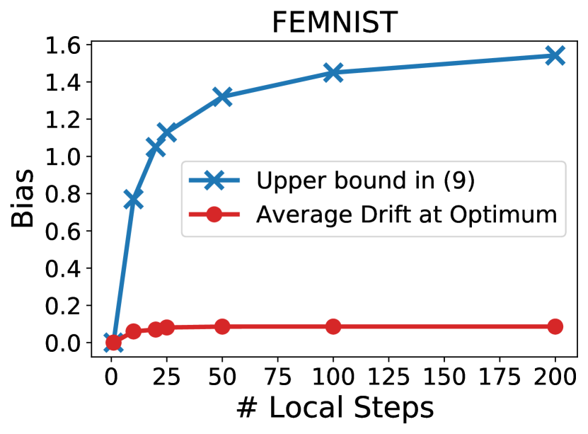
(a) FEMNIST.

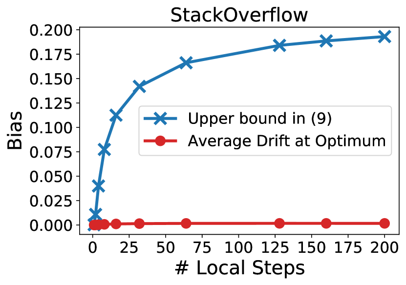
(b) StackOverflow.

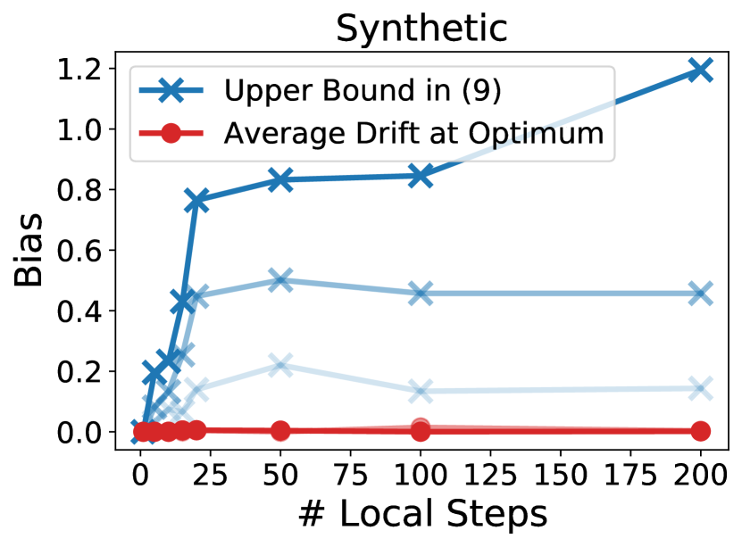
(c) Synthetic Dataset.

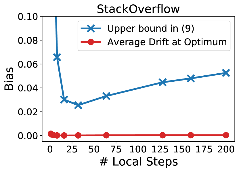
(d) StackOverflow. Stochastic local updates.

Figure 1: Gradient biases at the optimal point ${\bm{w}}^{*}$ on three different datasets. We observe that the average drift at optimum (i.e, norm of the gradient bias at ${\bm{w}}^{*}$, red line) nearly remain zero on all datasets but its upper bound 9 ($\mathbb{E}_{c}\|\nabla F_{c}({\bm{w}}^{*})-\mathcal{G}_{c}({\bm{w}}^{*})\|^{2}$, blue lines) slowly become larger when $H$ increases. In (c), different lines in the same color correspond to different levels of data heterogeneity. color=green!25, inline] Gauri: The names ’mean square’ and ’squared mean’ in the legend can be confusing to readers. Perhaps you can refer to the equations that define these terms? color=green!25, inline] Gauri: When you say different levels of gradient dissimilarity, is this a parameter that you choose, that is, the upper bound $\zeta$ on gradient dissimilarity? Or is it the actual gradient dissimilarity, the left side of (4)? color=green!25, inline] Gauri: If it is possible to drop one of these four plots, the remaining three will nicely fit in one row

Furthermore, we run FedAvg on FEMNIST dataset [17] following the same setup as [18] and check the values of the gradient bias at several intermediate points on the optimization trajectory. For each point, we let clients perform local GD with the same local learning rate for multiple steps. As shown in Figure 2, we observe a significant gap between the quantity of interest (i.e., the norm of average gradient bias, red lines) and its upper bound 9 (i.e., the average of $\ell_{2}$ norms, blue lines). Especially, at the $50$-th and $100$-th rounds, the upper bound 9 is about $10$ times larger. In addition, note that both the norm of average gradient bias and the average of $\ell_{2}$ norms only increase slowly with the number of local steps $H$ and saturate after certain threshold. However, the upper bound 10 uses a quadratic function of $H$ to estimate them. All the above observations suggest that the upper bounds based on the gradient dissimilarity are pessimistic in practice.

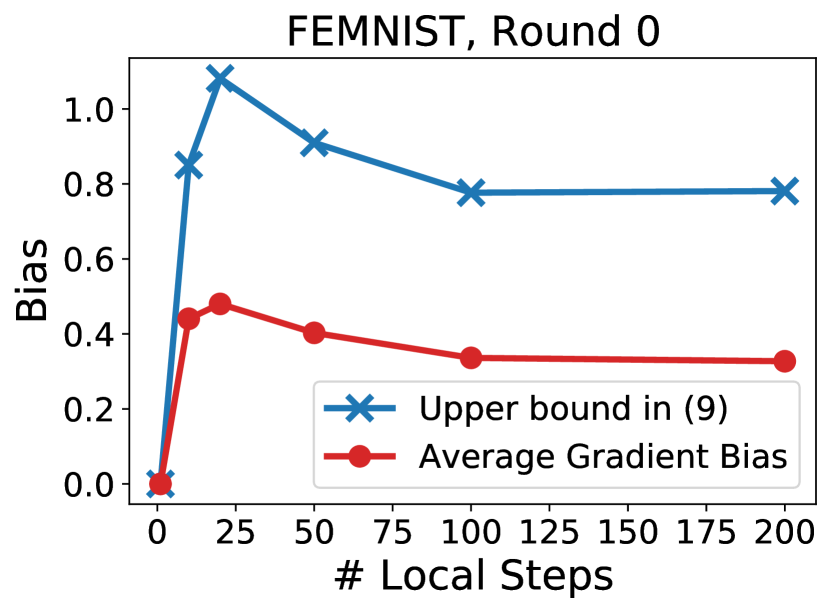
(a) Round 0.

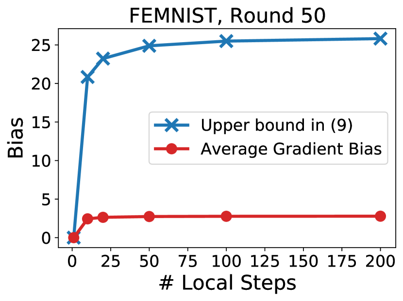
(b) Round 50.

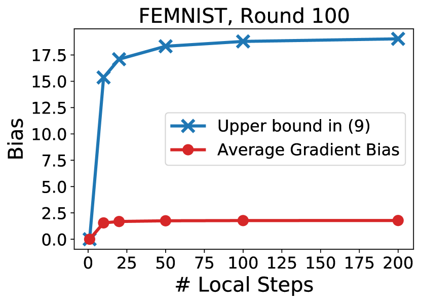
(c) Round 100.

Figure 2: Gradient biases at different points on a FedAvg’s optimization trajectory. There is a significant gap between the average gradient bias (red line) and its upper bound (blue lines). Both of them increase and then saturate when increasing $H$.

5 Convergence Analysis

In this section, we will provide a formal analysis (see Theorem 2) showing how the proposed measure of data heterogeneity, the average drift at optimum, influences the convergence of FedAvg. In particular, we provide convergence rates for strongly convex functions in Corollary 1, and for quadratic functions in Corollary 2. The results show that there exist regimes ($\rho\simeq 0$) where FedAvg enjoys the same rates in both homogeneous and heterogeneous data settings.

We first generalize the pseudo gradient in 5 to stochastic settings.

Definition 1 (Pseudo-Gradient).

Given ${\bm{w}}\in\mathbb{R}^{d}$, suppose ${\bm{w}}_{c,\text{GD}}^{(H)}$ and ${\bm{w}}_{c}^{(H)}$ denote the locally trained model on client $c$ after performing $H$ steps of GD and SGD using learning rate $\eta$, respectively. Then, we define

$$\text{Deterministic Pseudo-gradient:}\quad\mathcal{G}_{c}({\bm{w}}) \triangleq\frac{1}{\eta H}({\bm{w}}-{\bm{w}}_{c,\text{GD}}^{(H)}),$$ (17)

$$\text{Stochastic Pseudo-gradient:}\quad\hat{\mathcal{G}}_{c}({\bm{w}}) \triangleq\frac{1}{\eta H}({\bm{w}}-{\bm{w}}_{c}^{(H)}).$$ (18)

The average pseudo-gradients across all clients are defined as $\mathcal{G}=\mathbb{E}_{c}[\mathcal{G}_{c}]$ and $\hat{\mathcal{G}}=\mathbb{E}_{c}[\hat{\mathcal{G}_{c}}]$.

Instead of treating the stochastic pseudo-gradient 18 as a biased estimation of the original gradient $\nabla F_{c}({\bm{w}})$, we treat it as the biased version of 17. This new perspective allows us to extend previous analyses [3, 4, 16] to the stochastic setting and explicitly feature the impacts of average drift at optimum in the final error bound. Also, following many standard SGD analyses [6, 21], we assume the stochastic noise is upper bounded:

$$\mathbb{E}_{\xi}\left\|\nabla F_{c}({\bm{w}};\xi)-\nabla F_{c}({\bm{w}})\right\|^{2}\leq\sigma^{2}$$ (19)

where $\nabla F_{c}({\bm{w}};\xi)$ denotes the stochastic gradient with respect to a random mini-batch $\xi$.

5.1 Main Results

Given the definition of pseudo-gradients, we then derive the following theorem.

Theorem 2.

When each local objective function is $L$-Lipschitz smooth and $\mu$-strongly convex and the learning rates satisfy $\alpha\leq 1/4,\eta\leq\min\{1/L,1/\mu H\}$, after $T$ rounds of FedAvg (Local SGD), we have

$$\mathbb{E}\left\|{\bm{w}}^{(T)}-{\bm{w}}^{*}\right\|^{2}\leq (1-\frac{1}{2}\alpha\eta H\mu)^{T}\left\|{\bm{w}}^{(0)}-{\bm{w}}^{*}\right\|^{2}+\frac{2\alpha\eta H}{\mu}\max_{{\bm{w}}}\mathrm{Var}[\hat{\mathcal{G}}({\bm{w}})]$$

$$+\frac{20}{\mu^{2}}\max_{{\bm{w}}}\mathbb{E}_{c}\left\|\delta_{c}({\bm{w}})\right\|^{2}+\frac{20\rho^{2}}{\mu^{2}}$$ (20)

where $\rho$ denotes the average drift at optimum, $\mathbb{E}[\cdot],\mathrm{Var}[\cdot]$ are taken with respect to random noise in stochastic local updates, and $\delta_{c}({\bm{w}})=({\bm{w}}_{c,\text{GD}}^{(H)}-\mathbb{E}[{\bm{w}}_{c}^{(H)}])/(\eta H)$ denotes the iterate bias between local GD and local SGD on client $c$.

The Effects of Data Heterogeneity.

As shown in Theorem 2, the effects of data heterogeneity can be fully captured by the average drift at optimum $\rho$. Instead of providing a uniform upper bound for $\left\|\mathcal{G}({\bm{w}})-\nabla F({\bm{w}})\right\|$ like previous works, now we just need to ensure that $\rho=\left\|\mathcal{G}({\bm{w}}^{*})-\nabla F({\bm{w}}^{*})\right\|=\|\mathcal{G}({\bm{w}}^{*})\|$ is a small value. As we observed in our experimental results (see Figures 2 and 1), while $\left\|\mathcal{G}({\bm{w}})-\nabla F({\bm{w}})\right\|$ can be large, the value of average drift at optimum $\rho=\|\mathcal{G}({\bm{w}}^{*})\|$ is very close to zero on multiple realistic training tasks (FEMNIST, StackOverflow) for a reasonable range of $H$. In addition, in our proposed quadratic problem, one can prove that FedAvg implicitly ensures that for any $H$, we have $\rho\rightarrow 0$ almost surely as $M\rightarrow\infty$. All these observations suggest that it is possible that heterogeneous data on clients do not have negative impacts on the convergence due to $\rho\approx 0$. However, this important regime has not been investigated before.

The Effects of Stochastic Noise.

From Theorem 2, we can observe that the stochastic noise during local updates influences the second and the third terms on the right-hand-side of 20. The upper bounds of these two terms only depend on the dynamics of SGD algorithm, which has been well understood in literature. For example, in [11], the authors show that $\mathbb{E}\|{\bm{w}}^{(H)}-\mathbb{E}[{\bm{w}}^{(H)}]\|^{2}\leq 2\eta^{2}H\sigma^{2}$. As a consequence, we directly obtain that

$$\mathrm{Var}[\hat{\mathcal{G}}({\bm{w}})]=\frac{1}{M}\mathrm{Var}[\hat{\mathcal{G}}_{c}({\bm{w}})]=\frac{1}{\eta^{2}H^{2}M}\mathbb{E}\left\|{\bm{w}}_{c}^{(H)}-\mathbb{E}[{\bm{w}}_{c}^{(H)}]\right\|^{2}\leq\frac{2\sigma^{2}}{MH}.$$ (21)

As for the iterate bias, one can obtain

$$\mathbb{E}_{c}\left\|\delta_{c}({\bm{w}})\right\|^{2}\leq\eta^{2}L^{2}\sigma^{2}(H-1),$$ (22)

the proof of which is provided in the Appendix. After substituting 21 and 22 into 20 and optimizing the learning rates, we can obtain the following convergence rate for FedAvg.

Corollary 1 (Convergence Rate for Strongly Convex Functions).

Under the same setting as Theorem 2, when $\alpha=1/4,\eta={\mathcal{O}}(1/\mu HT)$, the convergence rate of FedAvg is

$$\mathbb{E}\left\|{\bm{w}}^{(T)}-{\bm{w}}^{*}\right\|^{2}=\widetilde{{\mathcal{O}}}\left(\frac{\sigma^{2}}{MHT}+\frac{\sigma^{2}}{HT^{2}}+\rho^{2}\right).$$ (23)

If clients perform local GD instead of local SGD, then when $\eta=\min\{1/L,1/(\mu H)\}$, we have

$$\left\|{\bm{w}}^{(T)}-{\bm{w}}^{*}\right\|^{2}={\mathcal{O}}\left(\exp\left(-\frac{T}{16\kappa}\min\{\kappa,H\}\right)+\rho^{2}\right)$$ (24)

where $\kappa=L/\mu$ denotes the condition number.

In the special regime of $\rho\approx 0$ (as in our proposed quadratic problem when $M\rightarrow\infty$, and empirical observations on multiple datasets), Corollary 1 states that, FedAvg has the same convergence rates in both homogeneous and heterogeneous data settings. As a result, data heterogeneity does not have negative impacts. However, in previous works based on gradient dissimilarity, even if $\rho=0$, there is an additional error. Moreover, in the deterministic setting, FedAvg’s rate ${\mathcal{O}}(\exp(-\mu HT/L))$ or ${\mathcal{O}}(\exp(-T))$ is strictly better than GD’s rate $\Omega(\exp(-\mu T/L))$ even in the presence of heterogeneous data. In contrast, as we discussed in Section 3.1, previous works can only get ${\mathcal{O}}(1/T^{2})$. A more detailed comparison with previous results is presented in Table 1.

Furthermore, it is worth noting that the idea of treating local updates as pseudo-gradients has appeared in [3, 4]. However, their analysis techniques require additional specialized assumptions about pseudo-gradients that can be difficult to satisfy, and they only considered deterministic FedAvg. Theorems 2 and 1 developed new techniques to analyze pseudo-gradients under common loss function assumptions in optimization, and showed they can be applied to the stochastic setting.

Algorithm	Worst-case error	Comm. rounds to attain $\epsilon$ error (when $\rho=0$)
GD	$\exp(-T/\kappa)$	${\mathcal{O}}(\kappa\log(1/\epsilon))$
FedAvg [12]	$\zeta^{2}/T^{2}$	${\mathcal{O}}(1/\epsilon^{2})$
FedAvg [26]	$1/(HT+H^{2}T^{2})+\zeta^{2}/T^{2}$	${\mathcal{O}}(1/\epsilon^{2})$
FedAvg (Ours)	$\exp(-T\min\{1,H/\kappa\})+\rho^{2}$	${\mathcal{O}}(\max\{1,\kappa/H\}\log(1/\epsilon))$

Table 1: Comparison with existing results for strongly convex objectives functions with deterministic local updates. In the table, the error is measured by the distance to the optimum $\|{\bm{w}}-{\bm{w}}^{*}\|^{2}$, and $\kappa=L/\mu$ is the condition number. Also, we omit logarithmic factors. Compared to previous results, we show that in the considered setting: (i) FedAvg enjoys linear convergence to the global optimum, and (ii) the multiple local steps of FedAvg mitigate the impact of of ill-conditioning (high condition number).

5.2 Extensions

Another benefit of using our analysis technique is that it allows us to easily incorporate additional assumptions. Below we provide several examples.

(1) Client Sampling: If we consider client sampling in FedAvg, then only the variance term in 20 will change and all other terms will not be affected at all. One can obtain new convergence guarantees by analyzing the variance of different sampling schemes and then simply substituting them into 20. Standard techniques to analyze client sampling [28] can be directly applied.

(2) Alternative Heterogeneity Assumptions: It is also possible to replace the data heterogeneity assumptions. Instead of setting the average drift at optimum $\rho$ to zero, one can also choose to apply the existing gradient dissimilarity technique to upper bound it. Alternatively, Hessian dissimilarity assumption ([10], $\|\nabla^{2}F_{c}({\bm{w}})-\nabla^{2}F({\bm{w}})\|\leq\beta$) may lead to an improved bound. We leave this extension to future work.

(3) Third-order Smoothness: When the local objective functions satisfy third-order smoothness ($\left\|\nabla^{2}F_{c}({\bm{w}})-\nabla^{2}F_{c}({\bm{u}})\right\|\leq Q\left\|{\bm{w}}-{\bm{u}}\right\|$), the bound of the iterate bias $\delta({\bm{w}})$ can be further improved while all other terms remain unchanged. According to [5], one can obtain $\left\|\delta({\bm{w}})\right\|\leq\frac{1}{4}\eta^{2}HQ\sigma^{2}$. In the special case when local objective functions are quadratic, we have $Q=0$. That is, there is no iterate bias. As a consequence, the convergence rate of FedAvg can be significantly improved. Specifically, we have the following formal corollary.

Corollary 2 (Convergence Rate for Quadratic Functions).

Suppose each local objective functions is quadratic. Then, the convergence rate of FedAvg with a fixed learning rate is given as follows:

$$\mathbb{E}\left\|{\bm{w}}^{(T)}-{\bm{w}}^{*}\right\|^{2}=\widetilde{{\mathcal{O}}}\left(\exp\left(-\frac{T}{16\kappa}\min\{\kappa,H\}\right)+\frac{\sigma^{2}}{MHT}+\rho^{2}\right).$$ (25)

color=red!25, inline]SK: Can we update the corollary to include dependence on $\rho$ similar to Corollary 1? Compared to Corollary 1 for strongly covnex functions, Corollary 2 gets an improved convergence rate due to the nice properties of quadratic functions. In the special case when $\rho=0$, FedAvg is strictly better than mini-batch SGD, which is $\widetilde{{\mathcal{O}}}(\exp(-T/\kappa)+\sigma^{2}/(MHT))$.

6 Concluding Remarks

In this paper, we aim at filling the gap between theory and practice about the convergence of the popular FedAvg algorithm. We found that previous analyses based on the bounded gradient dissimilarity assumption can be too pessimistic for practical applications. In order to accurately capture the effects data heterogeneity, we proposed a new measure, average drift at optimum, which remain close to zero across multiple real-world federated training tasks as well as our proposed quadratic problem, suggesting that data heterogeneity may have limited effect degrading FedAvg performance. At last, we provide a convergence analysis to illustrate how the average drift at optimum influences the convergence of FedAvg. The above new results can help to explain the empirical success of FedAvg. Future works may include extending the convergence analysis to general convex functions, and providing refined bounds for the average drift at optimum.

Appendix A Details of the Synthetic Dataset

The synthetic dataset we used in Figure 1 is constructed based on the statistical model proposed in Section 3.2. In particular, we set ${\bm{x}}_{c,i}\in\mathbb{R}^{d}$ to be a random vector, where $d=30$ and each element is sampled from a uniform distribution ${\mathcal{U}}(0,\nu_{c})$, $\nu_{c}\sim{\mathcal{U}}(0,5)$ is different on different clients. We assume there are total $M=100$ clients, each of which has $100$ data samples. Besides, we set $\epsilon_{c,i}\sim{\mathcal{N}}(0,0.09)$ and generate ${\bm{w}}^{*}$ from a distribution ${\mathcal{N}}(0,1)$. As we shown in 13, the gradient dissimilarity tightly depends on the scale of $\epsilon_{c,i}$. So we control the gradient dissimilarity via changing the variance of $\epsilon_{c,i}$.

Appendix B Proof of Lemma 1

Proof.

For the ease of writing, we define ${\bm{w}}^{+}={\bm{w}}^{(t+1)}$ and ${\bm{w}}={\bm{w}}^{(t)}$. Then, according to Lipschitz Smoothness and $\alpha\eta HL\leq 1$, we have

$$F({\bm{w}}^{+})\leq F({\bm{w}})-\alpha\eta H\left<\nabla F({\bm{w}}),\mathcal{G}({\bm{w}})\right>+\frac{\alpha^{2}\eta^{2}H^{2}L}{2}\left\|\mathcal{G}({\bm{w}})\right\|^{2}$$ (26)

$$= F({\bm{w}})-\frac{\alpha\eta H}{2}\left\|\nabla F({\bm{w}})\right\|^{2}+\frac{\alpha\eta H}{2}\left\|\nabla F({\bm{w}})-\mathcal{G}({\bm{w}})\right\|^{2}-\frac{\alpha\eta H}{2}(1-\alpha\eta HL)\left\|\mathcal{G}({\bm{w}})\right\|^{2}$$ (27)

$$\leq F({\bm{w}})-\frac{\alpha\eta H}{2}\left\|\nabla F({\bm{w}})\right\|^{2}+\frac{\alpha\eta H}{2}\left\|\nabla F({\bm{w}})-\mathcal{G}({\bm{w}})\right\|^{2}.$$ (28)

Besides, note that strongly convexity yields $\left\|\nabla F({\bm{w}})\right\|^{2}\geq 2\mu(F({\bm{w}})-F({\bm{w}}^{*}))$. So we have

$$F({\bm{w}}^{+})-F({\bm{w}}^{*})\leq\left(1-\alpha\eta H\mu\right)(F({\bm{w}})-F({\bm{w}}^{*}))+\frac{\alpha\eta H}{2}\left\|\nabla F({\bm{w}})-\mathcal{G}({\bm{w}})\right\|^{2}.$$ (29)

After total $T$ communication rounds, it follows that

$$F({\bm{w}}^{(T)})-F({\bm{w}}^{(*)})\leq\left(1-\alpha\eta H\mu\right)^{T}(F({\bm{w}}^{(0)})-F({\bm{w}}^{*}))+\frac{1}{2\mu T}\sum_{t=0}^{T-1}\left\|\nabla F({\bm{w}}^{(t)})-\mathcal{G}({\bm{w}}^{(t)})\right\|^{2}.$$ (30)

∎

Appendix C Proof of Theorem 1

Proof.

According to the local update rule, we have

$${\bm{w}}_{c}^{(t,h+1)}= {\bm{w}}_{c}^{(t,h)}-\eta\nabla F_{c}({\bm{w}}_{c}^{(t,h)})$$ (31)

$$= {\bm{w}}_{c}^{(t,h)}-\eta\left[{\bm{A}}_{c}({\bm{w}}_{c}^{(t,h)}-{\bm{w}}^{*})-{\bm{b}}_{c}\right]$$ (32)

$$= \left({\bm{I}}-\eta{\bm{A}}_{c}\right){\bm{w}}_{c}^{(t,h)}+\eta\left({\bm{A}}_{c}{\bm{w}}^{*}+{\bm{b}}_{c}\right).$$ (33)

Subtracting ${\bm{w}}_{c}^{*}={\bm{w}}^{*}+{\bm{A}}_{c}^{-1}{\bm{b}}_{c}$ on both sides, it follows that

$${\bm{w}}_{c}^{(t,h+1)}-{\bm{w}}_{c}^{*}= \left({\bm{I}}-\eta{\bm{A}}_{c}\right)\left({\bm{w}}_{c}^{(t,h)}-{\bm{w}}_{c}^{*}\right)$$ (34)

$$= \left({\bm{I}}-\eta{\bm{A}}_{c}\right)^{h+1}\left({\bm{w}}^{(t)}-{\bm{w}}_{c}^{*}\right).$$ (35)

Setting $h=H$, we have ${\bm{w}}_{c}^{(t,H)}=({\bm{I}}-\eta{\bm{A}}_{c})^{H}({\bm{w}}^{(t)}-{\bm{w}}_{c}^{*})+{\bm{w}}_{c}^{*}$. Recall the definition of pseudo-gradient 5, we get

$$\mathcal{G}_{c}({\bm{w}}^{(t)})= \frac{1}{\eta H}({\bm{w}}^{(t)}-{\bm{w}}^{(t,H)})$$ (36)

$$= \frac{1}{\eta H}\left[{\bm{I}}-({\bm{I}}-\eta{\bm{A}}_{c})^{H}\right]({\bm{w}}^{(t)}-{\bm{w}}^{*}_{c}).$$ (37)

According to the global update rule of FedAvg, one can obtain that

$${\bm{w}}^{(t+1)}= {\bm{w}}^{(t)}-\alpha\eta H\mathbb{E}_{c}\mathcal{G}_{c}({\bm{w}}^{(t)})$$ (38)

$$= {\bm{w}}^{(t)}-\alpha\mathbb{E}_{c}\left[({\bm{I}}-({\bm{I}}-\eta{\bm{A}}_{c})^{H})\left({\bm{w}}^{(t)}-{\bm{w}}_{c}^{*}\right)\right]$$ (39)

$$= {\bm{w}}^{(t)}-\alpha\mathbb{E}_{c}\left[({\bm{I}}-({\bm{I}}-\eta{\bm{A}}_{c})^{H})\left({\bm{w}}^{(t)}-{\bm{w}}^{*}\right)\right]$$

$$-\alpha\mathbb{E}_{c}\left[({\bm{I}}-({\bm{I}}-\eta{\bm{A}}_{c})^{H})\left({\bm{w}}^{*}-{\bm{w}}_{c}^{*}\right)\right].$$ (40)

Subtracting ${\bm{w}}^{*}$ on both sides and setting $\alpha=1$, we have

$${\bm{w}}^{(t+1)}-{\bm{w}}^{*}= \mathbb{E}_{c}\left[\left({\bm{I}}-\eta{\bm{A}}_{c}\right)^{H}\right]\left({\bm{w}}^{(t)}-{\bm{w}}^{*}\right)-\mathbb{E}_{c}\left[\underbrace{({\bm{I}}-({\bm{I}}-\eta{\bm{A}}_{c})^{H})\left({\bm{w}}^{*}-{\bm{w}}_{c}^{*}\right)}_{\eta H\mathcal{G}_{c}({\bm{w}}^{*})}\right]$$ (41)

$$= \mathbb{E}_{c}\left[\left({\bm{I}}-\eta{\bm{A}}_{c}\right)^{H}\right]\left({\bm{w}}^{(t)}-{\bm{w}}^{*}\right)-\eta H\mathcal{G}({\bm{w}}^{*})$$ (42)

where $\mathcal{G}({\bm{w}}^{*})=\mathbb{E}_{c}\mathcal{G}_{c}({\bm{w}}^{*})$. Assume that $\mathcal{G}({\bm{w}}^{*})=0$, then we have

$${\bm{w}}^{(t+1)}-{\bm{w}}^{*}=\left[\mathbb{E}_{c}\left[\left({\bm{I}}-\eta{\bm{A}}_{c}\right)^{H}\right]\right]^{t+1}({\bm{w}}^{(0)}-{\bm{w}}^{*}),$$ (43)

which proves the desired result.

In the following, we are going to prove $\mathcal{G}({\bm{w}}^{*})=0$ almost surely as $M\rightarrow\infty$ on this synthetic problem. According to the definition of ${\bm{A}}_{c},{\bm{b}}_{c}$, we obtain that

$$\mathcal{G}({\bm{w}}^{*})= \mathbb{E}_{c}\left[({\bm{I}}-({\bm{I}}-\eta{\bm{A}}_{c})^{H}){\bm{A}}_{c}^{-1}{\bm{b}}_{c}\right]$$ (44)

$$= \mathbb{E}_{c}\left[\underbrace{({\bm{I}}-({\bm{I}}-\eta{\bm{A}}_{c})^{H}){\bm{A}}_{c}^{-1}\frac{1}{n}\sum_{i=1}^{n}{\bm{x}}_{c,i}\epsilon_{c,i}}_{\xi_{c}}\right].$$ (45)

Since the noise $\epsilon_{c,\cdot}$ are independent of ${\bm{x}}_{c,\cdot}$, $\xi_{c}$ is a zero-mean random variable that depends on client $c$. Since we have assumed that all $\|{\bm{x}}_{c,i}\|$ and $\epsilon_{c,i}$ have bounded variance, we know that $\mathbb{E}[\xi_{c}^{2}]<\infty$. Since we have a uniform weighting on the $M$ clients, it follows $\mathbb{E}_{c}[\xi_{c}]=O(1/\sqrt{M})$ with probability $1-o_{M}(1)$, and as $M\to\infty$, we have $\mathbb{E}_{c}[\xi_{c}]\to 0$ almost surely.

∎

Appendix D Proof of Lemma 2

Before diving into the proof details, we would like to first introduce a lemma, which will be frequently used in the subsequent sections.

Lemma 3 (Mean Value Theorem).

Suppose function $F$ is twice differentiable, then

$$\nabla F_{c}({\bm{w}})-\nabla F_{c}({\bm{u}})={\bm{A}}_{c}({\bm{w}},{\bm{u}})\cdot({\bm{w}}-{\bm{u}})$$ (46)

where ${\bm{A}}_{c}({\bm{w}},{\bm{u}})=\int_{0}^{1}\nabla^{2}F_{c}({\bm{u}}+s({\bm{w}}-{\bm{u}}))\text{d}s$. If $\mu\preceq\nabla^{2}F_{c}\preceq L$, then it follows that $\mu\preceq{\bm{A}}_{c}({\bm{w}},{\bm{u}})\preceq L$ for any ${\bm{w}},{\bm{u}}$.

According to Lemma 3, for any local gradient at client $c$, we have

$$\nabla F_{c}({\bm{w}}^{(t,h+1)})= \nabla F_{c}({\bm{w}}^{(t,h)})+{\bm{B}}_{c}^{(t,h)}({\bm{w}}^{(t,h+1)}-{\bm{w}}^{(t,h)})$$ (47)

$$= ({\bm{I}}-\eta{\bm{B}}_{c}^{(t,h)})\nabla F_{c}({\bm{w}}^{(t,h)})$$ (48)

$$= \prod_{s=0}^{h}({\bm{I}}-\eta{\bm{B}}_{c}^{(t,s)})\nabla F_{c}({\bm{w}}^{(t)})$$ (49)

where ${\bm{B}}_{c}^{(t,h)}$ is an integral of the Hessian matrix. Then, recall the definition of pseudo-gradient 5, we have

$$\mathcal{G}_{c}({\bm{w}}^{(t)})= \frac{1}{H}\sum_{h=0}^{H-1}\nabla F_{c}({\bm{w}}^{(t,h)})$$ (50)

$$= \left[\frac{{\bm{I}}}{H}+\frac{1}{H}\sum_{h=1}^{H-1}\prod_{s=0}^{h-1}({\bm{I}}-\eta{\bm{B}}_{c}^{(t,s)})\right]\nabla F_{c}({\bm{w}}^{(t)}).$$ (51)

From 51, one can observe that the pseudo-gradient is a linear transformation of the local gradient at the starting point. As a result, we can write the average drift at optimum as follows:

$$\rho= \left\|\mathbb{E}_{c}[\mathcal{G}_{c}({\bm{w}}^{*})-\nabla F_{c}({\bm{w}}^{*})]\right\|$$ (52)

$$= \left\|\mathbb{E}_{c}\underbrace{\left[{\bm{I}}-\frac{{\bm{I}}}{H}-\frac{1}{H}\sum_{h=1}^{H-1}\prod_{s=0}^{h-1}({\bm{I}}-\eta{\bm{B}}_{c}^{(*,s)})\right]}_{{\bm{P}}_{c}}\nabla F_{c}({\bm{w}}^{*})\right\|.$$ (53)

When local objective functions are quadratic, we have ${\bm{B}}_{c}^{(*,s)}=\nabla^{2}F_{c}({\bm{w}}^{*})$ for any $s$. Accordingly, it follows that

$${\bm{P}}_{c}= {\bm{I}}-\frac{{\bm{I}}}{H}-\frac{1}{H}\sum_{h=1}^{H-1}\prod_{s=0}^{h-1}({\bm{I}}-\eta{\bm{B}}_{c}^{(*,s)})$$ (54)

$$= {\bm{I}}-\frac{1}{H}\sum_{h=0}^{H-1}({\bm{I}}-\eta\nabla^{2}F_{c}({\bm{w}}^{*}))^{h}$$ (55)

$$= \frac{1}{H}\sum_{h=0}^{H-1}\left[{\bm{I}}-({\bm{I}}-\eta\nabla^{2}F_{c}({\bm{w}}^{*}))^{h}\right].$$ (56)

Here we complete the proof.

Appendix E Proof of Theorem 2

E.1 Preliminaries

In this subsection, we will first introduce several useful lemmas, which relate to the properties of the deterministic pseudo-gradients.

Lemma 4 (Convexity, Smoothness & Co-coercivity).

When each local objective function $F_{c}$ is $L$-Lipschitz smooth and $\mu$-strongly convex, for any ${\bm{w}},{\bm{u}}\in\mathbb{R}^{d}$, we have

$$\widetilde{\mu}\left\|{\bm{w}}-{\bm{u}}\right\|^{2}\leq \left<\mathcal{G}({\bm{w}})-\mathcal{G}({\bm{u}}),{\bm{w}}-{\bm{u}}\right>\leq\widetilde{L}\left\|{\bm{w}}-{\bm{u}}\right\|^{2},$$ (57)

$$\left\|\mathcal{G}({\bm{w}})-\mathcal{G}({\bm{u}})\right\|^{2}\leq \widetilde{L}\left<\mathcal{G}({\bm{w}})-\mathcal{G}({\bm{u}}),{\bm{w}}-{\bm{u}}\right>,$$ (58)

where $\widetilde{\mu}=[1-(1-\eta\mu)^{H}]/(\eta H)$ and $\widetilde{L}=[1+(1-\eta\mu)^{H}]/(\eta H)$.

Proof.

Let us first focus on the pseudo-gradient on a specific client $c$. According to the definition of pseudo-gradient, we have

$$\eta H[\mathcal{G}_{c}({\bm{w}})-\mathcal{G}_{c}({\bm{u}})]= {\bm{w}}-{\bm{u}}-({\bm{w}}_{c}^{(H)}-{\bm{u}}_{c}^{(H)})$$ (59)

$$= {\bm{w}}-{\bm{u}}$$

$$-[{\bm{w}}_{c}^{(H-1)}-{\bm{u}}_{c}^{(H-1)}-\eta(\nabla F_{c}({\bm{w}}_{c}^{(H-1)})-\nabla F_{c}({\bm{u}}_{c}^{(H-1)}))]$$ (60)

$$= {\bm{w}}-{\bm{u}}-(I-\eta{\bm{D}}_{c}^{(H-1)})({\bm{w}}_{c}^{(H-1)}-{\bm{u}}_{c}^{(H-1)})$$ (61)

where 61 follows from Lemma 3 and ${\bm{D}}_{c}$ is a symmetric matrix satisfying $\mu\preceq{\bm{D}}_{c}\preceq L$. Repeating the above procedure, we can obtain that

$$\eta H[\mathcal{G}_{c}({\bm{w}})-\mathcal{G}_{c}({\bm{u}})]= {\bm{w}}-{\bm{u}}-\prod_{k=0}^{H-1}({\bm{I}}-\eta{\bm{D}}_{c}^{(k)})({\bm{w}}-{\bm{u}})$$ (62)

$$= \left[{\bm{I}}-\prod_{k=0}^{H-1}({\bm{I}}-\eta{\bm{D}}_{c}^{(k)})\right]({\bm{w}}-{\bm{u}}).$$ (63)

As a consequence, we have

$$\eta H\left<\mathcal{G}_{c}({\bm{w}})-\mathcal{G}_{c}({\bm{u}}),{\bm{w}}-{\bm{u}}\right>= \left\|{\bm{w}}-{\bm{u}}\right\|^{2}-\left<\prod_{k=0}^{H-1}({\bm{I}}-\eta{\bm{D}}_{c}^{(k)})({\bm{w}}-{\bm{u}}),{\bm{w}}-{\bm{u}}\right>.$$ (64)

Note that, due to Cauchy–Schwarz inequality,

$$\left|\left<\prod_{k=0}^{H-1}({\bm{I}}-\eta{\bm{D}}_{c}^{(k)})({\bm{w}}-{\bm{u}}),{\bm{w}}-{\bm{u}}\right>\right|\leq \prod_{k=0}^{H-1}\left\|{\bm{I}}-\eta{\bm{D}}_{c}^{(k)}\right\|\left\|{\bm{w}}-{\bm{u}}\right\|^{2}$$ (65)

$$\leq (1-\eta\mu)^{H}\left\|{\bm{w}}-{\bm{u}}\right\|^{2}.$$ (66)

That is,

$$-(1-\eta\mu)^{H}\left\|{\bm{w}}-{\bm{u}}\right\|^{2}\leq\left<\prod_{k=0}^{H-1}({\bm{I}}-\eta{\bm{D}}_{c}^{(k)})({\bm{w}}-{\bm{u}}),{\bm{w}}-{\bm{u}}\right>\leq(1-\eta\mu)^{H}\left\|{\bm{w}}-{\bm{u}}\right\|^{2}.$$ (67)

It follows that,

$$\frac{1-(1-\eta\mu)^{H}}{\eta H}\left\|{\bm{w}}-{\bm{u}}\right\|^{2}\leq\left<\mathcal{G}_{c}({\bm{w}})-\mathcal{G}_{c}({\bm{u}}),{\bm{w}}-{\bm{u}}\right>\leq\frac{1+(1-\eta\mu)^{H}}{\eta H}\left\|{\bm{w}}-{\bm{u}}\right\|^{2}.$$ (68)

Taking the average over all clients, we complete the proof of 57.

Next, we are going to prove 58. Note that

$$\left\|{\bm{w}}_{c}^{(H)}-{\bm{u}}_{c}^{(H)}\right\|= \left\|\prod_{k=0}^{H-1}({\bm{I}}-\eta{\bm{D}}_{c}^{(k)})({\bm{w}}-{\bm{u}})\right\|$$ (69)

$$\leq \prod_{k=0}^{H-1}\left\|{\bm{I}}-\eta{\bm{D}}_{c}^{(k)}\right\|\left\|{\bm{w}}-{\bm{u}}\right\|$$ (70)

$$\leq (1-\eta\mu)^{H}\left\|{\bm{w}}-{\bm{u}}\right\|.$$ (71)

As a result, we have

$$\left\|{\bm{w}}^{(H)}-{\bm{u}}^{(H)}\right\|^{2}=\left\|\mathbb{E}_{c}{\bm{w}}_{c}^{(H)}-\mathbb{E}_{c}{\bm{u}}_{c}^{(H)}\right\|^{2}\leq \mathbb{E}_{c}\left\|{\bm{w}}_{c}^{(H)}-{\bm{u}}_{c}^{(H)}\right\|^{2}$$ (72)

$$\leq [(1-\eta\mu)^{H}]^{2}\left\|{\bm{w}}-{\bm{u}}\right\|^{2}.$$ (73)

Then, according to the definition of pseudo-gradients, one can obtain

$$\eta^{2}H^{2}\left\|\mathcal{G}({\bm{w}})-\mathcal{G}({\bm{u}})\right\|^{2}= \left\|{\bm{w}}-{\bm{u}}-{\bm{w}}^{(H)}+{\bm{u}}^{(H)}\right\|^{2}$$ (74)

$$= \left\|{\bm{w}}-{\bm{u}}\right\|^{2}+\left\|{\bm{w}}^{(H)}-{\bm{u}}^{(H)}\right\|^{2}-2\left<{\bm{w}}-{\bm{u}},{\bm{w}}^{(H)}-{\bm{u}}^{(H)}\right>$$ (75)

$$\leq [1+(1-\eta\mu)^{H}]\left\|{\bm{w}}-{\bm{u}}\right\|^{2}-2\left<{\bm{w}}-{\bm{u}},{\bm{w}}^{(H)}-{\bm{u}}^{(H)}\right>$$

$$-(1-\eta\mu)^{H}\left[1-(1-\eta\mu)^{H}\right]\left\|{\bm{w}}-{\bm{u}}\right\|^{2}$$ (76)

$$= [1+(1-\eta\mu)^{H}]\left[\left\|{\bm{w}}-{\bm{u}}\right\|^{2}-\left<{\bm{w}}-{\bm{u}},{\bm{w}}^{(H)}-{\bm{u}}^{(H)}\right>\right]$$

$$-(1-(1-\eta\mu)^{H})\left<{\bm{w}}-{\bm{u}},{\bm{w}}^{(H)}-{\bm{u}}^{(H)}\right>$$

$$-(1-\eta\mu)^{H}\left[1-(1-\eta\mu)^{H}\right]\left\|{\bm{w}}-{\bm{u}}\right\|^{2}$$ (77)

$$= [1+(1-\eta\mu)^{H}]\left[\left\|{\bm{w}}-{\bm{u}}\right\|^{2}-\left<{\bm{w}}-{\bm{u}},{\bm{w}}^{(H)}-{\bm{u}}^{(H)}\right>\right]$$

$$+(1-(1-\eta\mu)^{H})\left[\left\|{\bm{w}}-{\bm{u}}\right\|^{2}-\left<{\bm{w}}-{\bm{u}},{\bm{w}}^{(H)}-{\bm{u}}^{(H)}\right>\right]$$

$$-\left[1+(1-\eta\mu)^{H}\right]\left[1-(1-\eta\mu)^{H}\right]\left\|{\bm{w}}-{\bm{u}}\right\|^{2}$$ (78)

Note that $\eta H\left<{\bm{w}}-{\bm{u}},\mathcal{G}({\bm{w}})-\mathcal{G}({\bm{u}})\right>=\left\|{\bm{w}}-{\bm{u}}\right\|^{2}-\left<{\bm{w}}-{\bm{u}},{\bm{w}}^{(H)}-{\bm{u}}^{(H)}\right>$ and $\eta H\widetilde{L}=1+(1-\eta\mu)^{H}$, $\eta H\widetilde{\mu}=1-(1-\eta\mu)^{H}$, we have

$$\left\|\mathcal{G}({\bm{w}})-\mathcal{G}({\bm{u}})\right\|^{2}\leq (\widetilde{L}+\widetilde{\mu})\left<{\bm{w}}-{\bm{u}},\mathcal{G}({\bm{w}})-\mathcal{G}({\bm{u}})\right>-\widetilde{L}\widetilde{\mu}\left\|{\bm{w}}-{\bm{u}}\right\|^{2}$$ (79)

$$= \widetilde{L}\left<{\bm{w}}-{\bm{u}},\mathcal{G}({\bm{w}})-\mathcal{G}({\bm{u}})\right>$$

$$-\widetilde{\mu}\left[\widetilde{L}\left\|{\bm{w}}-{\bm{u}}\right\|^{2}-\left<{\bm{w}}-{\bm{u}},\mathcal{G}({\bm{w}})-\mathcal{G}({\bm{u}})\right>\right]$$ (80)

$$\leq \widetilde{L}\left<{\bm{w}}-{\bm{u}},\mathcal{G}({\bm{w}})-\mathcal{G}({\bm{u}})\right>$$ (81)

where the last inequality is due to the smoothness of the pseudo-gradient 57. ∎

E.2 Main Proof

In the analysis below, we first analyze the training progress within one round. Suppose the current global model is ${\bm{w}}$ and the next round’s global model is ${\bm{w}}^{+}$. Without otherwise stated, the expectation $\mathbb{E}$ and variance $\mathrm{Var}$ are conditioned on the current global model ${\bm{w}}$. For the ease of writing, we define effective learning rate $\widetilde{\alpha}=\alpha\eta H$.

First, according to the update rule of FedAvg, we have

$$\mathbb{E}\left\|{\bm{w}}^{+}-{\bm{w}}^{*}\right\|^{2}= \mathbb{E}\left\|{\bm{w}}-\widetilde{\alpha}\hat{\mathcal{G}}({\bm{w}})-{\bm{w}}^{*}\right\|^{2}$$ (82)

$$= \left\|{\bm{w}}-\widetilde{\alpha}\mathbb{E}[\hat{\mathcal{G}}({\bm{w}})]-{\bm{w}}^{*}\right\|^{2}+\widetilde{\alpha}^{2}\mathrm{Var}[\hat{\mathcal{G}}({\bm{w}})]$$ (83)

$$= \left\|{\bm{w}}-{\bm{w}}^{*}\right\|^{2}+\widetilde{\alpha}^{2}\left\|\mathbb{E}[\hat{\mathcal{G}}({\bm{w}})]\right\|^{2}-2\widetilde{\alpha}\left<{\bm{w}}-{\bm{w}}^{*},\mathbb{E}[\hat{\mathcal{G}}({\bm{w}})]\right>+\widetilde{\alpha}^{2}\mathrm{Var}[\hat{\mathcal{G}}({\bm{w}})]$$ (84)

Also, note that $\mathbb{E}[\hat{\mathcal{G}}({\bm{w}})]=\mathcal{G}({\bm{w}})-\mathcal{G}({\bm{w}}^{*})+\mathcal{G}({\bm{w}}^{*})+\delta({\bm{w}})$. So one can obtain

$$\mathbb{E}\left\|{\bm{w}}^{+}-{\bm{w}}^{*}\right\|^{2}\leq \left\|{\bm{w}}-{\bm{w}}^{*}\right\|^{2}+2\widetilde{\alpha}^{2}\left\|\mathcal{G}({\bm{w}})-\mathcal{G}({\bm{w}}^{*})\right\|^{2}-2\widetilde{\alpha}\left<{\bm{w}}-{\bm{w}}^{*},\mathcal{G}({\bm{w}})-\mathcal{G}({\bm{w}}^{*})\right>$$

$$+2\widetilde{\alpha}^{2}\left\|\mathcal{G}({\bm{w}}^{*})+\delta({\bm{w}})\right\|^{2}-2\widetilde{\alpha}\left<{\bm{w}}-{\bm{w}}^{*},\mathcal{G}({\bm{w}}^{*})+\delta({\bm{w}})\right>+\widetilde{\alpha}^{2}\mathrm{Var}[\hat{\mathcal{G}}({\bm{w}})]$$ (85)

$$\leq (1-\widetilde{\alpha}\widetilde{\mu})\left\|{\bm{w}}-{\bm{w}}^{*}\right\|^{2}+2\widetilde{\alpha}^{2}\left\|\mathcal{G}({\bm{w}})-\mathcal{G}({\bm{w}}^{*})\right\|^{2}-\widetilde{\alpha}\left<{\bm{w}}-{\bm{w}}^{*},\mathcal{G}({\bm{w}})-\mathcal{G}({\bm{w}}^{*})\right>$$

$$+2\widetilde{\alpha}^{2}\left\|\mathcal{G}({\bm{w}}^{*})+\delta({\bm{w}})\right\|^{2}-2\widetilde{\alpha}\left<{\bm{w}}-{\bm{w}}^{*},\mathcal{G}({\bm{w}}^{*})+\delta({\bm{w}})\right>+\widetilde{\alpha}^{2}\mathrm{Var}[\hat{\mathcal{G}}({\bm{w}})]$$ (86)

where the first inequality uses the fact $\left\|a+b\right\|^{2}\leq 2\left\|a\right\|^{2}+2\left\|b\right\|^{2}$, and the second inequality comes from the strongly-convexity of the pseudo-gradient. Now let us check the value of the following terms:

$$T_{1}= 2\widetilde{\alpha}\left\|\mathcal{G}({\bm{w}})-\mathcal{G}({\bm{w}}^{*})\right\|^{2}-\left<{\bm{w}}-{\bm{w}}^{*},\mathcal{G}({\bm{w}})-\mathcal{G}({\bm{w}}^{*})\right>-2\left<{\bm{w}}-{\bm{w}}^{*},\mathcal{G}({\bm{w}}^{*})+\delta({\bm{w}})\right>.$$ (87)

According to the co-coercivity of the pseudo-gradient, we have

$$T_{1}\leq \left[2\widetilde{\alpha}\widetilde{L}-1\right]\left<{\bm{w}}-{\bm{w}}^{*},\mathcal{G}({\bm{w}})-\mathcal{G}({\bm{w}}^{*})\right>-2\left<{\bm{w}}-{\bm{w}}^{*},\mathcal{G}({\bm{w}}^{*})+\delta({\bm{w}})\right>$$ (88)

$$\leq \left[2\widetilde{\alpha}\widetilde{L}-1\right]\left<{\bm{w}}-{\bm{w}}^{*},\mathcal{G}({\bm{w}})-\mathcal{G}({\bm{w}}^{*})\right>+\epsilon\left\|{\bm{w}}-{\bm{w}}^{*}\right\|^{2}+\frac{1}{\epsilon}\left\|\mathcal{G}({\bm{w}}^{*})+\delta({\bm{w}})\right\|^{2}$$ (89)

where the last inequality comes from Young’s inequality. When $\widetilde{\alpha}\widetilde{\mu}\leq\widetilde{\alpha}\widetilde{L}\leq 1/4$, we have

$$T_{1}\leq-\frac{\widetilde{\mu}}{2}\left\|{\bm{w}}-{\bm{w}}^{*}\right\|^{2}+\epsilon\left\|{\bm{w}}-{\bm{w}}^{*}\right\|^{2}+\frac{1}{\epsilon}\left\|\mathcal{G}({\bm{w}}^{*})+\delta({\bm{w}})\right\|^{2}\leq\frac{2\left\|\mathcal{G}({\bm{w}}^{*})+\delta({\bm{w}})\right\|^{2}}{\widetilde{\mu}}$$ (90)

where the last inequality is obtained by setting $\epsilon=\widetilde{\mu}/2$. Then, substituting 90 into 86 and noting that $\widetilde{\alpha}\widetilde{\mu}\leq\widetilde{\alpha}\widetilde{L}\leq 1/4$ (that is, $\widetilde{\alpha}\leq 1/(4\widetilde{\mu})$),

$$\mathbb{E}\left\|{\bm{w}}^{+}-{\bm{w}}^{*}\right\|^{2}\leq (1-\widetilde{\alpha}\widetilde{\mu})\left\|{\bm{w}}-{\bm{w}}^{*}\right\|^{2}+\left(2\widetilde{\alpha}^{2}+\frac{2\widetilde{\alpha}}{\widetilde{\mu}}\right)\left\|\mathcal{G}({\bm{w}}^{*})+\delta({\bm{w}})\right\|^{2}+\widetilde{\alpha}^{2}\mathrm{Var}[\hat{\mathcal{G}}({\bm{w}})]$$ (91)

$$\leq (1-\widetilde{\alpha}\widetilde{\mu})\left\|{\bm{w}}-{\bm{w}}^{*}\right\|^{2}+\frac{5\widetilde{\alpha}}{2\widetilde{\mu}}\left\|\mathcal{G}({\bm{w}}^{*})+\delta({\bm{w}})\right\|^{2}+\widetilde{\alpha}^{2}\mathrm{Var}[\hat{\mathcal{G}}({\bm{w}})]$$ (92)

$$\leq (1-\widetilde{\alpha}\widetilde{\mu})\left\|{\bm{w}}-{\bm{w}}^{*}\right\|^{2}+\widetilde{\alpha}^{2}\mathrm{Var}[\hat{\mathcal{G}}({\bm{w}})]+\frac{5\widetilde{\alpha}}{\widetilde{\mu}}\left\|\delta({\bm{w}})\right\|^{2}+\frac{5\widetilde{\alpha}}{\widetilde{\mu}}\left\|\mathcal{G}({\bm{w}}^{*})\right\|^{2}$$ (93)

$$\leq (1-\widetilde{\alpha}\widetilde{\mu})\left\|{\bm{w}}-{\bm{w}}^{*}\right\|^{2}+\widetilde{\alpha}^{2}\max_{{\bm{w}}}\mathrm{Var}[\hat{\mathcal{G}}({\bm{w}})]$$

$$+\frac{5\widetilde{\alpha}}{\widetilde{\mu}}\max_{{\bm{w}}}\left\|\delta({\bm{w}})\right\|^{2}+\frac{5\widetilde{\alpha}}{\widetilde{\mu}}\left\|\mathcal{G}({\bm{w}}^{*})\right\|^{2}$$ (94)

After total $T$ communication rounds and taking the total expectation, we end up with

$$\mathbb{E}\left\|{\bm{w}}^{(T)}-{\bm{w}}^{*}\right\|^{2}\leq (1-\widetilde{\alpha}\widetilde{\mu})^{T}\left\|{\bm{w}}^{(0)}-{\bm{w}}^{*}\right\|^{2}+\frac{\widetilde{\alpha}}{\widetilde{\mu}}\max_{{\bm{w}}}\mathrm{Var}[\hat{\mathcal{G}}({\bm{w}})]$$

$$+\frac{5}{\widetilde{\mu}^{2}}\max_{{\bm{w}}}\mathbb{E}_{c}\left\|\delta_{c}({\bm{w}})\right\|^{2}+\frac{5\rho^{2}}{\widetilde{\mu}^{2}}.$$ (95)

When $\eta H\mu\leq 1$, one can easily validate that

$$\widetilde{\mu}=\frac{1-(1-\eta\mu)^{H}}{\eta H}\geq\frac{\mu}{2}.$$ (96)

So it follows that

$$\mathbb{E}\left\|{\bm{w}}^{(T)}-{\bm{w}}^{*}\right\|^{2}\leq (1-\frac{1}{2}\alpha\eta H\mu)^{T}\left\|{\bm{w}}^{(0)}-{\bm{w}}^{*}\right\|^{2}+\frac{2\alpha\eta H}{\mu}\max_{{\bm{w}}}\mathrm{Var}[\hat{\mathcal{G}}({\bm{w}})]$$

$$+\frac{20}{\mu^{2}}\max_{{\bm{w}}}\mathbb{E}_{c}\left\|\delta_{c}({\bm{w}})\right\|^{2}+\frac{20\rho^{2}}{\mu^{2}}.$$ (97)

At last, in order to satisfy $\widetilde{\alpha}\widetilde{L}\leq 1/4$, one can set $\alpha\leq 1/8$, such that

$$\widetilde{\alpha}\widetilde{L}=\alpha\eta H\cdot\frac{1+(1-\eta\mu)^{H}}{\eta H}=\alpha(1+(1-\eta\mu)^{H})\leq 2\alpha\leq\frac{1}{4}.$$ (98)

Appendix F Bound on Iterate Bias

In this section, we will provide an upper bound for the iterate bias 22. According to the local update rules, we have

$$\left\|{\bm{w}}_{c,\text{GD}}^{(H)}-\mathbb{E}[{\bm{w}}_{c}^{(H)}]\right\|= \left\|{\bm{w}}_{c,\text{GD}}^{(H-1)}-\mathbb{E}[{\bm{w}}_{c}^{(H-1)}]-\eta\nabla F_{c}({\bm{w}}_{c,\text{GD}}^{(H-1)})+\eta\mathbb{E}[\nabla F_{c}({\bm{w}}_{c}^{(H-1)})]\right\|$$ (99)

$$\leq \left\|{\bm{w}}_{c,\text{GD}}^{(H-1)}-\mathbb{E}[{\bm{w}}_{c}^{(H-1)}]-\eta\nabla F_{c}({\bm{w}}_{c,\text{GD}}^{(H-1)})+\eta\nabla F_{c}(\mathbb{E}[{\bm{w}}_{c}^{(H-1)}])\right\|$$

$$+\eta\left\|\mathbb{E}[\nabla F_{c}({\bm{w}}_{c}^{(H-1)})]-\nabla F_{c}(\mathbb{E}[{\bm{w}}_{c}^{(H-1)}])\right\|$$ (100)

$$\leq (1-\eta\mu)\left\|{\bm{w}}_{c,\text{GD}}^{(H-1)}-\mathbb{E}[{\bm{w}}_{c}^{(H-1)}]\right\|$$

$$+\eta\left\|\mathbb{E}[\nabla F_{c}({\bm{w}}_{c}^{(H-1)})]-\nabla F_{c}(\mathbb{E}[{\bm{w}}_{c}^{(H-1)}])\right\|$$ (101)

For the second term, we have

$$\left\|\mathbb{E}[\nabla F_{c}({\bm{w}}_{c}^{(H-1)})]-\nabla F_{c}(\mathbb{E}[{\bm{w}}_{c}^{(H-1)}])\right\|^{2}\leq \mathbb{E}\left\|\nabla F_{c}({\bm{w}}_{c}^{(H-1)})-\nabla F_{c}(\mathbb{E}[{\bm{w}}_{c}^{(H-1)}])\right\|^{2}$$ (102)

$$\leq L^{2}\mathbb{E}\left\|{\bm{w}}_{c}^{H-1}-\mathbb{E}[{\bm{w}}_{c}^{(H-1)}]\right\|^{2}$$ (103)

$$\leq 2\eta^{2}L^{2}\sigma^{2}(H-1)$$ (104)

where the last inequality comes from previous works [11, 5]. As a result, one can obtain

$$\left\|{\bm{w}}_{c,\text{GD}}^{(H)}-\mathbb{E}[{\bm{w}}_{c}^{(H)}]\right\|\leq (1-\eta\mu)\left\|{\bm{w}}_{c,\text{GD}}^{(H-1)}-\mathbb{E}[{\bm{w}}_{c}^{(H-1)}]\right\|+\sqrt{2}\eta^{2}L\sigma(H-1)^{\frac{1}{2}}$$ (105)

$$\leq \sqrt{2}\eta^{2}L\sigma\sum_{h=0}^{H-1}(1-\eta\mu)^{H-1-h}h^{\frac{1}{2}}$$ (106)

$$\leq \sqrt{2}\eta^{2}L\sigma\left[\sum_{h=0}^{H-1}(1-\eta\mu)^{2(H-1-h)}\right]^{\frac{1}{2}}\left[\sum_{h=0}^{H-1}h\right]^{\frac{1}{2}}$$ (107)

$$\leq \sqrt{2}\eta^{2}L\sigma\left[\sum_{h=0}^{H-1}(1-\eta\mu)^{H-1-h}\right]^{\frac{1}{2}}\left[\sum_{h=0}^{H-1}h\right]^{\frac{1}{2}}$$ (108)

$$= \left[\frac{1-(1-\eta\mu)^{H}}{\eta\mu H}\right]^{\frac{1}{2}}\eta^{2}L\sigma H(H-1)^{\frac{1}{2}}.$$ (109)

According to the definition of $\delta({\bm{w}})$, we obtain

$$\mathbb{E}_{c}\left\|\delta_{c}({\bm{w}})\right\|^{2}\leq\mathbb{E}_{c}\left\|{\bm{w}}_{c,\text{GD}}^{(H)}-\mathbb{E}[{\bm{w}}_{c}^{(H)}]\right\|^{2}\leq \frac{\widetilde{\mu}\eta^{2}L^{2}\sigma^{2}(H-1)}{\mu}\leq\eta^{2}L^{2}\sigma^{2}(H-1)$$ (110)

where the last inequality comes from the fact that $\widetilde{\mu}\leq\mu$.

Appendix G Proof of Corollary 1

G.1 Deterministic Setting

When clients perform local GD in each round, there is no stochastic noise. So the error upper bound 20 can be simplified as follows

$$\left\|{\bm{w}}^{(T)}-{\bm{w}}^{*}\right\|^{2}\leq(1-\frac{1}{2}\alpha\eta H\mu)^{T}\left\|{\bm{w}}^{(0)}-{\bm{w}}^{*}\right\|^{2}+\frac{20\rho^{2}}{\mu^{2}}.$$ (111)

If $H\mu\geq L$, then the maximal learning rate is $\eta=1/H\mu$. When $\alpha=1/8$, the upper bound becomes

$$\left\|{\bm{w}}^{(T)}-{\bm{w}}^{*}\right\|^{2}\leq \left(1-\frac{1}{16}\right)^{T}\left\|{\bm{w}}^{(0)}-{\bm{w}}^{*}\right\|^{2}+\frac{20\rho^{2}}{\mu^{2}}$$ (112)

$$\leq \exp\left(-\frac{T}{16}\right)\left\|{\bm{w}}^{(0)}-{\bm{w}}^{*}\right\|^{2}+\frac{20\rho^{2}}{\mu^{2}}.$$ (113)

If $H\mu\leq L$, then the maximal learning rate is $\eta=1/L$. When $\alpha=1/8$, the upper bound becomes

$$\left\|{\bm{w}}^{(T)}-{\bm{w}}^{*}\right\|^{2}\leq \left(1-\frac{H\mu}{16L}\right)^{T}\left\|{\bm{w}}^{(0)}-{\bm{w}}^{*}\right\|^{2}+\frac{20\rho^{2}}{\mu^{2}}$$ (114)

$$\leq \exp\left(-\frac{\mu HT}{16L}\right)\left\|{\bm{w}}^{(0)}-{\bm{w}}^{*}\right\|^{2}+\frac{20\rho^{2}}{\mu^{2}}.$$ (115)

We can summarize the above two bounds as follows:

$$\left\|{\bm{w}}^{(T)}-{\bm{w}}^{*}\right\|^{2}\leq \exp\left(-\frac{T}{16\kappa}\min\{\kappa,H\}\right)\left\|{\bm{w}}^{(0)}-{\bm{w}}^{*}\right\|^{2}+\frac{20\rho^{2}}{\mu^{2}}$$ (116)

$$= {\mathcal{O}}\left(\exp\left(-\frac{T}{16\kappa}\min\{\kappa,H\}\right)+\rho^{2}\right).$$ (117)

G.2 Stochastic Setting

Substituting the upper bounds for $\mathrm{Var}[\mathcal{G}({\bm{w}})]$ and $\delta({\bm{w}})$ into Section E.2 and setting $\alpha=1/8$,

$$\mathbb{E}\left\|{\bm{w}}^{(t+1)}-{\bm{w}}^{*}\right\|^{2}\leq (1-\widetilde{\alpha}\widetilde{\mu})\left\|{\bm{w}}^{(t)}-{\bm{w}}^{*}\right\|^{2}+\widetilde{\alpha}^{2}\frac{2\sigma^{2}}{MH}+\frac{5\widetilde{\alpha}^{3}}{\widetilde{\mu}}\frac{\sigma^{2}L^{2}(H-1)}{\alpha^{2}H^{2}}+\frac{5\widetilde{\alpha}}{\widetilde{\mu}}\left\|\mathcal{G}({\bm{w}}^{*})\right\|^{2}$$ (118)

$$\leq (1-\widetilde{\alpha}\widetilde{\mu})\left\|{\bm{w}}^{(t)}-{\bm{w}}^{*}\right\|^{2}+\widetilde{\alpha}^{2}\frac{2\sigma^{2}}{MH}+\widetilde{\alpha}^{3}\frac{320\sigma^{2}L^{2}}{\widetilde{\mu}H}+\widetilde{\alpha}\frac{5\rho^{2}}{\widetilde{\mu}}.$$ (119)

After minor rearrangement, we can get

$$\mathbb{E}\left\|{\bm{w}}^{(t+1)}-{\bm{w}}^{*}\right\|^{2}-\frac{5\rho^{2}}{\widetilde{\mu}^{2}}\leq(1-\widetilde{\alpha}\widetilde{\mu})\left[\left\|{\bm{w}}^{(t)}-{\bm{w}}^{*}\right\|^{2}-\frac{5\rho^{2}}{\widetilde{\mu}^{2}}\right]+\widetilde{\alpha}^{2}\frac{2\sigma^{2}}{MH}+\widetilde{\alpha}^{3}\frac{320\sigma^{2}L^{2}}{\widetilde{\mu}H}.$$ (120)

After total $T$ communication rounds,

$$\mathbb{E}\left\|{\bm{w}}^{(t+1)}-{\bm{w}}^{*}\right\|^{2}-\frac{5\rho^{2}}{\widetilde{\mu}^{2}}\leq(1-\widetilde{\alpha}\widetilde{\mu})^{T}\underbrace{\left[\left\|{\bm{w}}^{(0)}-{\bm{w}}^{*}\right\|^{2}-\frac{5\rho^{2}}{\widetilde{\mu}^{2}}\right]}_{r_{0}}+\frac{2\widetilde{\alpha}\sigma^{2}}{\widetilde{\mu}MH}+\frac{320\widetilde{\alpha}^{2}\sigma^{2}L^{2}}{\widetilde{\mu}^{2}H}.$$ (121)

If we set $\widetilde{\alpha}=\frac{\nu}{\mu T}$, where $\nu=2\ln(\max\{r_{0}\mu^{2}MHT/(8\sigma^{2}),r_{0}\mu^{4}HT^{2}/(1280L^{2}\sigma^{2})\})$, then it follows that

$$\mathbb{E}\left\|{\bm{w}}^{(t+1)}-{\bm{w}}^{*}\right\|^{2}-\frac{20\rho^{2}}{\mu^{2}}\leq \frac{8\sigma^{2}\nu}{\mu^{2}MHT}+\frac{1280\sigma^{2}L^{2}\nu}{\mu^{4}HT^{2}}+\exp\left(-\frac{\nu}{2}\right)r_{0}$$ (122)

$$\leq \frac{8\sigma^{2}(\nu+1)}{\mu^{2}MHT}+\frac{1280\sigma^{2}L^{2}(\nu+1)}{\mu^{4}HT^{2}}$$ (123)

$$= \widetilde{{\mathcal{O}}}\left(\frac{\sigma^{2}}{MHT}+\frac{\sigma^{2}}{HT^{2}}\right)$$ (124)

where $\widetilde{{\mathcal{O}}}$ omits the logarithmic factors.

Appendix H Proof of Corollary 2

In the quadratic setting, the iterate bias is zero. So from Section E.2, we get

$$\mathbb{E}\left\|{\bm{w}}^{(t+1)}-{\bm{w}}^{*}\right\|^{2}-\frac{5\rho^{2}}{\widetilde{\mu}^{2}}\leq (1-\widetilde{\alpha}\widetilde{\mu})\left[\left\|{\bm{w}}^{(t)}-{\bm{w}}^{*}\right\|^{2}-\frac{5\rho^{2}}{\widetilde{\mu}^{2}}\right]+\widetilde{\alpha}^{2}\frac{2\sigma^{2}}{MH}.$$ (125)

Then, taking the total expectation on both sides, for the $T$-th round, we have

$$\mathbb{E}\left\|{\bm{w}}^{(T)}-{\bm{w}}^{*}\right\|^{2}-\frac{5\rho^{2}}{\widetilde{\mu}^{2}}\leq (1-\widetilde{\alpha}\widetilde{\mu})^{T}\left[\left\|{\bm{w}}^{(0)}-{\bm{w}}^{*}\right\|^{2}-\frac{5\rho^{2}}{\widetilde{\mu}^{2}}\right]+\frac{2\widetilde{\alpha}\sigma^{2}}{\widetilde{\mu}MH}$$ (126)

According to [21], with some constant learning rate $\widetilde{\alpha}={\mathcal{O}}(1/\widetilde{\mu}T)$, one can directly obtain

$$\mathbb{E}\left\|{\bm{w}}^{(t+1)}-{\bm{w}}^{*}\right\|^{2}-\frac{5\rho^{2}}{\widetilde{\mu}^{2}}=\widetilde{{\mathcal{O}}}\left(\exp\left(-\widetilde{\mu}\widetilde{\alpha}_{\text{max}}T\right)+\frac{2\sigma^{2}}{\widetilde{\mu}^{2}MHT}\right).$$ (127)

where $\widetilde{{\mathcal{O}}}$ omits the logarithmic factors. In addition, note that $\eta\leq\min\{1/(\mu H),1/L\}$. Accordingly, $\widetilde{\alpha}_{\max}=\min\{1/8,\mu H/(8L)\}$ and $\widetilde{\mu}>\mu/2$. As a consequence,

$$\mathbb{E}\left\|{\bm{w}}^{(t+1)}-{\bm{w}}^{*}\right\|^{2}= \widetilde{{\mathcal{O}}}\left(\exp\left(-\frac{T}{16\kappa}\min\{\kappa,H\}\right)+\frac{8\sigma^{2}}{\mu^{2}MHT}+\frac{20\rho^{2}}{\mu^{2}}\right)$$ (128)

$$= \widetilde{{\mathcal{O}}}\left(\exp\left(-\frac{T}{16\kappa}\min\{\kappa,H\}\right)+\frac{\sigma^{2}}{MHT}+\rho^{2}\right).$$ (129)

References

- [1] M. Assran, N. Loizou, N. Ballas, and M. Rabbat. Stochastic gradient push for distributed deep learning. arXiv preprint arXiv:1811.10792, 2018.
- [2] Z. Charles, Z. Garrett, Z. Huo, S. Shmulyian, and V. Smith. On large-cohort training for federated learning. Advances in Neural Information Processing Systems, 34, 2021.
- [3] Z. Charles and J. Konečnỳ. Convergence and accuracy trade-offs in federated learning and meta-learning. In International Conference on Artificial Intelligence and Statistics, pages 2575–2583. PMLR, 2021.
- [4] Z. Charles and K. Rush. Iterated vector fields and conservatism, with applications to federated learning. In International Conference on Algorithmic Learning Theory, pages 130–147. PMLR, 2022.
- [5] M. Glasgow, H. Yuan, and T. Ma. Sharp bounds for federated averaging (local sgd) and continuous perspective. arXiv preprint arXiv:2111.03741, 2021.
- [6] R. M. Gower, N. Loizou, X. Qian, A. Sailanbayev, E. Shulgin, and P. Richtárik. Sgd: General analysis and improved rates. In International Conference on Machine Learning, pages 5200–5209. PMLR, 2019.
- [7] F. Haddadpour and M. Mahdavi. On the convergence of local descent methods in federated learning. arXiv preprint arXiv:1910.14425, 2019.
- [8] T.-M. H. Hsu, H. Qi, and M. Brown. Measuring the effects of non-identical data distribution for federated visual classification. arXiv preprint arXiv:1909.06335, 2019.
- [9] P. Kairouz, H. B. McMahan, B. Avent, A. Bellet, M. Bennis, A. N. Bhagoji, K. Bonawitz, Z. Charles, G. Cormode, R. Cummings, et al. Advances and open problems in federated learning. arXiv preprint arXiv:1912.04977, 2019.
- [10] S. P. Karimireddy, S. Kale, M. Mohri, S. J. Reddi, S. U. Stich, and A. T. Suresh. SCAFFOLD: Stochastic controlled averaging for on-device federated learning. In Proceedings of the International Conference on Machine Learning, 2020.
- [11] A. Khaled, K. Mishchenko, and P. Richtárik. Tighter theory for local SGD on identical and heterogeneous data. In Proceedings of the Twenty Third International Conference on Artificial Intelligence and Statistics, 2020.
- [12] A. Koloskova, N. Loizou, S. Boreiri, M. Jaggi, and S. U. Stich. A unified theory of decentralized SGD with changing topology and local updates. In International Conference on Machine Learning, 2020.
- [13] T. Li, A. K. Sahu, M. Zaheer, M. Sanjabi, A. Talwalkar, and V. Smith. Federated optimization in heterogeneous networks. In Proceedings of the Conference on Machine Learning and Systems, 2020.
- [14] X. Li, K. Huang, W. Yang, S. Wang, and Z. Zhang. On the convergence of fedavg on non-iid data. arXiv preprint arXiv:1907.02189, 2019.
- [15] X. Lian, C. Zhang, H. Zhang, C.-J. Hsieh, W. Zhang, and J. Liu. Can decentralized algorithms outperform centralized algorithms? a case study for decentralized parallel stochastic gradient descent. In Advances in Neural Information Processing Systems, pages 5336–5346, 2017.
- [16] G. Malinovskiy, D. Kovalev, E. Gasanov, L. Condat, and P. Richtarik. From local sgd to local fixed-point methods for federated learning. In International Conference on Machine Learning, pages 6692–6701. PMLR, 2020.
- [17] H. B. McMahan, E. Moore, D. Ramage, S. Hampson, et al. Communication-efficient learning of deep networks from decentralized data. In Proceedings of the 20th International Conference on Artificial Intelligence and Statistics, 2017.
- [18] S. Reddi, Z. Charles, M. Zaheer, Z. Garrett, K. Rush, J. Konečnỳ, S. Kumar, and H. B. McMahan. Adaptive federated optimization. arXiv preprint arXiv:2003.00295, 2020.
- [19] S. J. Reddi, S. Kale, and S. Kumar. On the convergence of adam and beyond. arXiv preprint arXiv:1904.09237, 2019.
- [20] S. U. Stich. Local SGD converges fast and communicates little. In Proceedings of the International Conference on Learning Representations (ICLR), 2019.
- [21] S. U. Stich. Unified optimal analysis of the (stochastic) gradient method. arXiv preprint arXiv:1907.04232, 2019.
- [22] J. Wang, Z. Charles, Z. Xu, G. Joshi, H. B. McMahan, M. Al-Shedivat, G. Andrew, S. Avestimehr, K. Daly, D. Data, et al. A field guide to federated optimization. arXiv preprint arXiv:2107.06917, 2021.
- [23] J. Wang and G. Joshi. Cooperative SGD: A unified framework for the design and analysis of communication-efficient SGD algorithms. arXiv preprint arXiv:1808.07576, 2018.
- [24] J. Wang, Q. Liu, H. Liang, G. Joshi, and H. V. Poor. Tackling the objective inconsistency problem in heterogeneous federated optimization. Advances in Neural Information Processing Systems, 33, 2020.
- [25] J. Wang, V. Tantia, N. Ballas, and M. Rabbat. SlowMo: Improving communication-efficient distributed SGD with slow momentum. In Proceedings of the International Conference on Learning Representations (ICLR), 2020.
- [26] B. Woodworth, K. K. Patel, and N. Srebro. Minibatch vs local sgd for heterogeneous distributed learning. arXiv preprint arXiv:2006.04735, 2020.
- [27] B. Woodworth, K. K. Patel, S. U. Stich, Z. Dai, B. Bullins, H. B. McMahan, O. Shamir, and N. Srebro. Is local SGD better than minibatch SGD? In International Conference on Machine Learning, 2020.
- [28] H. Yang, M. Fang, and J. Liu. Achieving linear speedup with partial worker participation in non-iid federated learning. In International Conference on Learning Representations, 2020.
- [29] H. Yu, R. Jin, and S. Yang. On the linear speedup analysis of communication efficient momentum SGD for distributed non-convex optimization. In International Conference on Machine Learning, 2019.
- [30] H. Yu, S. Yang, and S. Zhu. Parallel restarted SGD with faster convergence and less communication: Demystifying why model averaging works for deep learning. In Proceedings of the AAAI Conference on Artificial Intelligence, volume 33, pages 5693–5700, 2019.
- [31] K. Yuan, Q. Ling, and W. Yin. On the convergence of decentralized gradient descent. SIAM Journal on Optimization, 26(3):1835–1854, 2016.
- [32] F. Zhou and G. Cong. On the convergence properties of a k-step averaging stochastic gradient descent algorithm for nonconvex optimization. In Proceedings of the 27th International Joint Conference on Artificial Intelligence (IJCAI), pages 3219–3227, 2018.