Consistent Estimation of Multiple Breakpoints in Dependence Measures

This paper proposes different methods to consistently detect multiple breaks in copula-based dependence measures, mainly focusing on Spearman’s $\rho$. The leading model is a factor copula model due to its usefulness for analyzing data in high dimensions. Starting with the classical binary segmentation, also the more recent wild binary segmentation (WBS) and a procedure based on an information criterion are considered. For all procedures, consistency of the estimators for the location of the breakpoints as well as the number of breaks is proved. Monte Carlo simulations indicate that WBS performs best in many, but not in all, situations. A real data application on recent Euro Stoxx 50 data reveals the usefulness of the procedures.

Keywords: (Wild) Binary Segmentation, Factor Copula, Information Criterion

1 Introduction

For asset allocation in financial markets and risk management purposes, dependence measures are of great interest. For example, it is necessary to estimate the variance-covariance matrix of asset returns to construct mean-variance efficient portfolios as introduced by Markowitz, (1952). In recent years, also copula-based/non-linear dependencies Nelsen, (2006, Chapter 5) became popular, e.g. using a conditional multivariate version of Spearman’s $\rho$ as in Schmid and Schmidt, (2007) or Penzer et al., (2012). Therefore, estimators of these measures are crucial. However, in financial time series, breaks in dependence measures can occur. These happen quite frequently in times of crisis, e.g. during the financial crisis in 2008 or more recently in the beginning of 2020 when the Corona pandemic began. This phenomenon is generally known as the diversification meltdown. Hence, consistent estimation of the location of those break points as well as their number need to be considered in order to correctly estimate the dependencies between assets (in between the breaks).

In this paper, we propose methods for dating multiple breaks in copula-based dependence measures. The methods are broadly applicable, but our leading example is the factor copula framework as introduced in Oh and Patton, (2017). This is especially useful in high-dimensional applications due to the sparse amount of parameters in the factor structure. Abstaining from a multivariate Gaussian distribution assumption, it can capture tail risk as well as the leverage effect. Breakpoint detection in a factor copula framework has already discussed been discussed by Manner et al., (2019). We extend their so-called ‘moment-based’ test to the detection of multiple breakpoints in copula-based dependence measures for filtered data. In doing so, we use recent results by Nasri et al., (2022) to derive consistency of our procedure for the location as well as the number of breaks from primitive conditions.

The literature for structural changes in dependence measures is wide. Wied et al., 2012b , for instance, test for breaks in the correlation using an extended functional delta method, while Aue et al., (2009) test for changes in the covariance matrix. Nonlinear dependence measures like Spearman’s $\rho$ are analyzed with respect to break points in Gombay and Horváth, (1999), Wied et al., (2014), Kojadinovic et al., (2016), Manner et al., (2019), or Stark and Otto, (2022), among others. Similar to Wied et al., (2014), we use a CUSUM-type statistic but allow for multiple copula-based dependence measures including, for example, Spearman’s $\rho$, Gini’s $\gamma$, or Spearman’s footrule. However, we follow suggestions by Bücher et al., (2014) for calculating ranks sequentially to improve power. Moreover, our test statistic is based on filtered return data instead of observable time series; an idea also recently employed by Barassi et al., (2020) to analyze changes in the conditional correlation.

In order to detect multiple breaks, we use a binary segmentation (BS) algorithm that goes back to Vostrikova, (1981) and which since then has been adopted frequently in the literature; see, e.g. Bai, (1997). In principle, we follow the algorithm used in Galeano and Tsay, (2009) or in Galeano and Wied, (2014). More specifically, the maximum of a CUSUM-statistic within the subintervals is compared to some critical value. Here, and similar to Bai and Perron, (1998, Section 4.3), we derive the asymptotic distribution of the maximum statistic under the null hypothesis that there is no additional break to take multiple testing into account. We also extend our results to the wild binary segmentation (WBS) algorithm of Fryzlewicz, (2014), which improves the detection of change points, especially for multiple breaks in close proximity.

The rest of this paper is structured as follows. Section 2 contains the copula-based dependence measures, segmentation algorithms and the consistency results. In Section 3 Monte Carlo simulations are provided. Section 4 gives an empirical application, while Section 5 concludes.

2 Finding Multiple Breaks in Dependence Measures

2.1 Modeling Breaks in Dependence Measures

Suppose we observe a sample $\bm{Y}_{1},\dots,\bm{Y}_{T}$ of length $T$ with a cross section $\bm{Y}_{t}\coloneqq(Y_{1,t},\dots,Y_{n,t})^{\prime}$ of $n$ financial assets so that each $n\times 1$ vector $\bm{Y}_{t}$, $t\in\{1,\dots,T\}$, obeys a parametric location-scale specification

$$\bm{Y}_{t}=\bm{\mu}_{t}(\bm{\phi}^{0})+\bm{\sigma}_{t}(\bm{\phi}^{0})\bm{\eta}_{t},$$ (1)

where $\bm{\eta}_{t}\coloneqq(\eta_{1,t},\dots,\eta_{n,T})^{\prime}$ are innovations with $\textsf{E}[\eta_{i,t}]=0$ and $\textsf{var}[\eta_{i,t}]=1$ for any $i\in\{1,\dots,n\}$. Similar to Chen and Fan, (2006), Oh and Patton, (2013), and Oh and Patton, (2017), we assume that the conditional mean and variance functions—respectively given by $\bm{\mu}_{t}(\bm{\phi}^{0})\coloneqq(\mu_{1,t}(\bm{\phi}^{0}),\dots,\mu_{n,t}(\bm{\phi}^{0}))^{\prime}$ and $\bm{\sigma}_{t}(\bm{\phi}^{0})\coloneqq\textsf{diag}\{\sigma_{1,t}(\bm{\phi}^{0}),\dots,\sigma_{n,t}(\bm{\phi}^{0})\}$—are (a) parametrically known up to a finite dimensional parameter $\bm{\phi}^{0}$ and (b) measurable with respect to $\mathcal{F}_{t-1}\coloneqq\sigma(\{\bm{Y}_{j},\,j<t\})$. The innovations $\bm{\eta}_{t}$, on the other hand, are jointly independent of $\mathcal{F}_{t-1}$. This setting allows for many AR-GARCH specifications commonly encountered in financial econometrics.

Assuming continuous margins $\textsf{F}_{i,t}(x)\coloneqq\textsf{P}(\eta_{i,t}\leq x)$, $x\in\mathbb{R}$, we can rephrase the conditional joint distribution as

$$\bm{Y}_{t}\mid\mathcal{F}_{t-1}\sim\textsf{C}_{t}(\textsf{F}_{1,t}(\eta_{1,t}),\dots,\textsf{F}_{n,t}(\eta_{n,t})),$$ (2)

where the copula $\textsf{C}_{t}(\bm{u})=\textsf{P}(\bm{U}_{t}\leq\bm{u}),$ $\bm{u}\in[0,1]^{n}$, $\bm{U}_{t}\coloneqq(U_{1,t},\dots,U_{n,t})^{\prime}$ with $U_{i,t}\coloneqq\textsf{F}_{i,t}(\eta_{i,t})$, captures uniquely the dependence among the $n$ variates in $\bm{\eta}_{t}$; see Patton, (2006). In what follows, we aim at finding change points in certain dependence measures that can be solely expressed in terms of the copula. As argued, for example, in Bücher et al., (2014) or Kojadinovic et al., (2016), classical nonparametric tests based on sequential empirical processes have little power against alternatives that leave the margins unchanged and only involve a change in the copula.

More specifically, for a finite collection of disjoint sets $\{\mathcal{G}_{1},\dots,\mathcal{G}_{G}\}$ partitioning the cross-sectional index set $\{1,\dots,n\}$ and a collection of suitable bivariate functions $h_{l}:[0,1]^{2}\rightarrow\mathbb{R}$, $l\in\{1,\dots,H\}$, we focus on averaged rank-based dependence measures of the type

$$m_{t,g,l}\coloneqq\frac{1}{\displaystyle{|\mathcal{G}_{g}|\choose 2}}\mathop{\sum}\limits_{\begin{subarray}{c}1\leq i<j\leq n\\ i,j\,\in\,\mathcal{G}_{g}\end{subarray}}m_{i,j,t,l},\;m_{i,j,t,l}\coloneqq\textsf{E}[h_{l}(U_{i,t},U_{j,t})],\,g\in\{1,\dots,G\}.$$ (3)

We aim at locating and estimating change points of the $p\times 1$ vector

$$\bm{m}_{t}\coloneqq(\bm{m}_{t,1}^{\prime},\dots,\bm{m}_{t,G}^{\prime})^{\prime},\;\bm{m}_{t,g}\coloneqq(m_{t,g,1},\dots,m_{t,g,H})^{\prime},\;\;p\coloneqq GH.$$

To illustrate, Spearman’s $\rho$, Spearman’s footrule ($\varrho$), and Gini’s $\gamma$ fit into this setup with $h_{\rho}(u,v)=12uv-3$, $h_{\varrho}(u,v)=1-3|u-v|$, and $h_{\gamma}(u,v)=2(|u+v-1|-|u-v|)$ for $(u,v)\in[0,1]^{2}$, respectively; see, e.g., Nelsen, (2006). The group structure is often used in empirical studies, where some degree of homogeneity within each group can be expected so that $m_{i,j,t,l}=m_{g,t,l}$ for all $(i,j)\in\mathcal{G}_{g}$. Group structures are commonly used in empirical work; see, e.g. Oh and Patton, (2017), Opschoor et al., (2021), or Oh and Patton, (2021). Averaged dependence measures are used frequently and have been found to perform well; see, e.g. Schmid and Schmidt, (2007), Quessy, (2009), Kojadinovic et al., (2016), or Manner et al., (2019).

Importantly, the above-mentioned dependence measures do not depend on the univariate margins, i.e.

$$m_{i,j,t,l}=\int_{[0,1]^{2}}h_{l}(u,v)\,\textsf{d}\textsf{C}_{i,j,t}(u,v),$$ (4)

where $\textsf{C}_{i,j,t}(u_{i},u_{j})\coloneqq\textsf{C}_{t}(\bm{u}^{(i,j}))$, with $\bm{u}^{(i,j)}=(1,\dots,1,u_{i},1,\dots,1,u_{j},1\dots,1)^{\prime}$ for some $n\times 1$ vector $\bm{u}\in[0,1]^{n}$, denotes the bivariate marginal copula of $\textsf{C}_{t}$. A change in $\bm{m}_{t}$ over time must thus be due to a change in $\textsf{C}_{t}$. We therefore consider the following break-point scenario as summarized by Assumption A.

Assumption A

The following holds true:

1. Consider a finite partition $0\eqqcolon z_{0}^{0}<z_{1}^{0}<\dots<z_{\ell^{0}}^{0}<z_{\ell^{0}+1}^{0}\coloneqq 1$. If $\lfloor z_{i-1}^{0}T\rfloor\leq\lfloor t/T\rfloor\leq\lfloor z_{i}^{0}T\rfloor$, $i\in\{1,\dots,\ell^{0}+1\}$, then $\textsf{C}_{t}(\bm{u})=\textsf{C}_{i}(\bm{u})$, where $\textsf{C}_{1},\dots,\textsf{C}_{\ell^{0}+1}$ denote copulae, which are pairwise different in at least one point $\bm{u}\in[0,1]^{n}$ such that $\bm{m}_{t}=\bm{g}(t/T)$, where $\bm{g}:[0,1]\rightarrow\mathbb{R}^{p}$ is a vector-valued step function defined as

   $$\bm{g}(z)=\sum_{i\,=\,0}^{\ell^{0}}\bm{\gamma}_{i}^{0}1\{z\,\in\,[z_{i}^{0},z_{i+1}^{0})\},\,\,\bm{g}(1)\coloneqq\bm{\gamma}_{\ell^{0}}^{0}.$$

   The $p\times 1$ level vectors $\bm{\gamma}_{0}^{0},\dots,\bm{\gamma}_{\ell^{0}}^{0}$, as well as $z_{1}^{0},\dots,z_{\ell^{0}}^{0}$ and $\ell^{0}$ are finite constants independent of $T$.

2. The partial derivatives $\dot{\textsf{C}}_{i,k+1}\coloneqq\partial\textsf{C}_{k+1}/\partial{u_{i}}$ exist and are continuous on $\{\bm{u}\in[0,1]^{n}:0<u_{i}<1\}$, for any $k\in\{0,1,\dots,\ell^{0}\}$ and $i\in\{1,\dots,n\}$.

3. $\bm{\eta}_{1},\dots,\bm{\eta}_{T}$ is a sample from a process $\{\bm{\eta}_{t}\}_{t\,\in\,\mathbb{Z}}$ of independently distributed $n\times 1$ random vectors $\bm{\eta}_{t}=(\eta_{1,t},\dots,\eta_{n,t})^{\prime}$ with strictly stationary and continuous univariate margins $\eta_{i,t}\sim\textsf{F}_{i}$, $i\in\{1,\dots,n\}$.

The function $\bm{g}(\cdot)$ defined in part (A1) of Assumption A specifies the timing and the size of the changes in the dependence measures. This specification is tailored towards abrupt changes and allows for a change in only a subset of $\bm{m}_{t}$; see Galeano and Wied, (2014, 2017) for a detailed discussion. Part (A2) is due to Segers, (2012) and imposes a smoothness condition on the partial derivatives of the copula. Similar to Bücher et al., (2014) or Kojadinovic et al., (2016), by imposing part (A3) of Assumption A, we maintain stationary marginal distributions, i.e. the joint distribution is only affected by a break in the copula. The following remark illustrates the setting within the context of factor copulas.

Remark 1.

Recently, factor copula models gained some popularity as a parsimonious yet flexible way to model the cross-sectional dependence among a possibly large number of financial assets; see, e.g. Oh and Patton, (2013), Krupskii and Joe, (2013), Creal and Tsay, (2015), or Opschoor et al., (2021). According to this literature, one may assume that the unknown copula $\textsf{C}_{t}$ governing Eq. (2) can be generated from an auxiliary factor model of the form $X_{i,t}=\beta_{i,t}Z_{t}+\varepsilon_{i,t}$, where $Z_{t}$, $\beta_{i,t}$, and $\varepsilon_{i,t}$ denote factor, factor loading, and idiosyncratic component, respectively. For example, the group structure mentioned above arises naturally within the ‘block-equidependence’ model from Oh and Patton, (2017) where assets are driven by some latent market factor with different intensity in each group/industry resulting in equal dependence between the assets in each group but different dependence across groups. Breaks in dependence measures could result from structural changes in loadings, i.e. if $\beta_{i,t}\neq\beta_{i,t+1}$ for some $t\in\{1,\dots,T\}$; an issue investigated below in more detail.

2.2 Segmentation Algorithms

Suppose $\hat{\bm{\phi}}$ is a $\sqrt{T}$-consistent estimator of $\bm{\phi}^{0}$ so that we can define the residuals $\hat{\eta}_{i,t}\coloneqq\sigma_{i,t}^{-1}(\hat{\bm{\phi}})(Y_{i,t}-\mu_{i,t}(\hat{\bm{\phi}}))$. Moreover, for any $1\leq k<m\leq T$, let $\hat{U}_{i,t}^{k:m}$, $i\in\{1,\dots,n\}$, $t\in\{k,\dots,m\}$, denote the rank of $\hat{\eta}_{i,t}$ among $\hat{\eta}_{i,k},\dots,\hat{\eta}_{i,m}$. We then define for any $[a,b]\subseteq[0,1]$, a sample analogue of (3) by

$$\hat{m}_{g,l}^{\lfloor aT\rfloor+1:\lfloor bT\rfloor}\coloneqq\frac{1}{\displaystyle{|\mathcal{G}_{g}|\choose 2}}\mathop{\sum}\limits_{\begin{subarray}{c}1\leq i<j\leq n\\ i,j\,\in\,\mathcal{G}_{g}\end{subarray}}\hat{m}_{i,j,l}^{\lfloor aT\rfloor+1:\lfloor bT\rfloor},\,l\in\{1,\dots,H\},\,g\in\{1,\dots,G\},$$ (5)

where

$$\hat{m}_{i,j,l}^{\lfloor aT\rfloor+1:\lfloor bT\rfloor}\coloneqq\frac{1}{\lfloor bT\rfloor-\lfloor aT\rfloor}\sum_{t\,=\,\lfloor aT\rfloor+1}^{\lfloor bT\rfloor}h_{l}(\hat{U}_{i,t}^{\lfloor aT\rfloor+1:\lfloor bT\rfloor},\hat{U}_{j,t}^{\lfloor aT\rfloor+1:\lfloor bT\rfloor}),$$

so that we obtain the $p\times 1$ vector $\hat{\bm{m}}^{\lfloor aT\rfloor+1:\lfloor bT\rfloor}\coloneqq(\hat{\bm{m}}_{1}^{\lfloor aT\rfloor+1:\lfloor bT\rfloor}{}^{\prime},\dots,\hat{\bm{m}}_{G}^{\lfloor aT\rfloor+1:\lfloor bT\rfloor}{}^{\prime})^{\prime}$, where $\hat{\bm{m}}_{g}^{\lfloor aT\rfloor+1:\lfloor bT\rfloor}\coloneqq(\hat{m}_{g,1}^{\lfloor aT\rfloor+1:\lfloor bT\rfloor},\dots,\hat{m}_{g,H}^{\lfloor aT\rfloor+1:\lfloor bT\rfloor})^{\prime}$. Next, define for a given interval $[a,b]\subseteq[0,1]$ with $0\leq\lfloor aT\rfloor<\lfloor bT\rfloor\leq T$, the detector

$$\hat{M}(a,b;z)=\,\frac{\lfloor zT\rfloor-\lfloor aT\rfloor}{\sqrt{\lfloor bT\rfloor-\lfloor aT\rfloor}}\left\|\hat{\bm{m}}^{\lfloor aT\rfloor+1:\lfloor zT\rfloor}-\hat{\bm{m}}^{\lfloor aT\rfloor+1:\lfloor bT\rfloor}\right\|_{2},$$

and the fluctuation test statistic

$$\hat{M}(a,b)\coloneqq\operatorname*{\textsf{sup}}_{z\,\in\,[a,b]}\hat{M}(a,b;z)=\operatorname*{\textsf{max}}_{z\,\in\,\Pi_{T}(a,b)}\hat{M}(a,b;z),$$ (6)

where $\Pi_{T}(a,b)\coloneqq\{\lfloor aT\rfloor/T,(\lfloor aT\rfloor+1)/T,\dots,(\lfloor bT\rfloor-1)/T,\lfloor bT\rfloor/T\}$, $\|\cdot\|_{2}$ is the Euclidean norm, and the conventions $\hat{M}(a,b;z)=0$ if $z=a$ and $\Pi_{T}\coloneqq\Pi_{T}(0,1)$ are used.

Equation (6) can be related to the test statistic used in Wied et al., (2014) up to a scaling factor for $h=h_{\rho}$ and $H=1$. However, they calculate the ranks for Spearman’s $\rho$ for the subset $[1,\dots,k]$ relative to the complete sample in contrast to our approach basing it only on the subset. Bücher et al., (2014) and Kojadinovic et al., (2016) provide empirical evidence showing more powerful results using ranks computed relative to the subset; see also Manner et al., (2019) for an application. The aforementioned papers all use averaged dependence measures as well while we allow for multiple averaged dependencies in several groups.

2.2.1 Binary Segmentation

The following break-point detection algorithm is closely related to the segmentation algorithms proposed by Galeano and Tsay, (2009), Galeano and Wied, (2014, 2017), which, in turn, are based on the seminal work of Vostrikova, (1981). For a given upper tail probability $\alpha$, the maximum of the test statistic from Eq. (6) is evaluated over $\ell+1$ subintervals and then compared to some critical value $c_{\alpha}(\ell)$, which depends on the amount of breaks $\ell$ already found and which is formally derived from Proposition 2 below. This way, the issue of multiple testing is taken into account similar to the procedure in Bai and Perron, (1998, Section 4.3). More formally, the algorithm can be summarized by the following two steps:

1. Obtain from Eq. (6) the test statistics $\hat{M}(0,1)$.

   1. If the test statistic is statistically significant, i.e. if $\hat{M}_{0,1}>c_{\alpha}(0)$, where $c_{\alpha}(0)$ is the asymptotic critical value $c_{\alpha}(\ell)$ from Proposition 2 below with $\ell=0$ for a given upper tail probability $\alpha$, then a change is announced. Let $z_{1}=\operatorname*{\textsf{arg\,max}}\limits_{z\,\in\,\Pi_{T}}\hat{M}(0,1;z)$ be the break point estimator and go to Step 2.

   2. If the test statistic is not statistically significant, the algorithm stops, and no change points are detected.

2. Let $z_{1},\dots,z_{\ell}$ be the $\ell$ change points in increasing order already found in previous iterations and $z_{0}\coloneqq 0$, $z_{\ell+1}\coloneqq 1$. If

   $$\operatorname*{\textsf{max}}\limits_{1\,\leq\,k\,\leq\,\ell+1}\hat{M}(z_{k-1},z_{k})>c_{\alpha}(\ell),$$

   then a new change point is detected at the point fraction at which the value $\hat{M}(z_{k_{\textsf{max}-1}},z_{k_{\textsf{max}}})$ is attained, where

   $$k_{\textsf{max}}=\operatorname*{\textsf{arg\,max}}\limits_{1\,\leq\,k\,\leq\,\ell+1}\hat{M}(z_{k-1},z_{k}).$$

   Repeat this step until no more change points are found.

In other words, the whole data set is scanned for a change point, once a significant change point is found, the data set is split at that point. On the resulting subsamples the test statistic is computed again and the maximum is then compared to the according critical value. If the associated change point is significant the sample is split again at that point. This procedure stops when no significant change points can be found. This is also done in Galeano and Tsay, (2009) and Galeano and Wied, (2014). A slightly different approach considering the subsamples seperately can be found in Venkatraman, (1992), Bai, (1997), Aue et al., (2009), Fryzlewicz, (2014), among others. Evidently, binary segmentation is commonly done in order to extend single change point detection procedures to multiple change point detection.

2.2.2 Analytical Results

In order to derive the asymptotic properties of the algorithm from Section 2.2.1, we impose the following assumptions.

Assumption B

For any $[a,b]\subseteq[0,1]$, the function $M(a,b;\cdot):[a,b]\rightarrow\mathbb{R}_{+}$, $z\mapsto M(a,b;z)$, where $M(a,b;z)\coloneqq\lVert\bm{M}(a,b;z)\rVert_{2}$, with

$$\bm{M}(a,b;z)=\frac{1}{b-a}\left(\int_{a}^{z}\bm{g}(t)\,\textnormal{{d}}t-\frac{z-a}{b-a}\int_{a}^{b}\bm{g}(t)\,\textnormal{{d}}t\right),$$

is either constant or has a unique maximum.

Assumption C

For any $l\in\{1,\dots,H\}$, the following holds true.

1. $h_{l}:[0,1]^{2}\rightarrow\mathbb{R}$ is of bounded variation in the sense of Hardy-Krause.

2. $h_{l}:[0,1]^{2}\rightarrow\mathbb{R}$ is Lipschitz; i.e., for any $(u_{1},v_{1})\in[0,1]^{2}$ and $(u_{2},v_{2})\in[0,1]^{2}$, $|h_{l}(u_{1},v_{1})-h_{l}(u_{2},v_{2})|\leq c_{0}(|u_{1}-u_{2}|+|v_{1}-v_{2}|)$ for some constant $c_{0}\in(0,\infty)$.

Assumption B is similar to Galeano and Wied, (2014, Assumption 2) and Galeano and Wied, (2017, Assumption 7), and restricts the nature of the breaks. Assumption B is fulfilled if there is a ‘dominating’ break in any subset of components at the same time point. For examples where the assumption is fulfilled or violated see Galeano and Wied, (2014) for the case that $\bm{g}(t)$ is a scalar. To provide some intuition, note that, as shown in the appendix, the function $M(a,b;z)$, specified in Assumption B, coincides with the probability limit of the scaled detector, i.e. $|\hat{M}(a,b;z)/\sqrt{\lfloor bT\rfloor-\lfloor aT\rfloor}-M(a,b;z)|=o_{p}(1)$ uniformly on $[a,b]$. Assumption C is satisfied by the above-mentioned dependence measures. Part (C1) enables the use of an integration by parts formula for bivariate integrals; see, e.g. Fermanian et al., (2004) and Berghaus et al., (2017); part (C2) is a convenient assumption, which, however, rules out certain dependence measures like quantile dependence.

In order to discuss the next assumption, it is convenient to first introduce the unfeasible sequential empirical copula process

$$\tilde{\mathbb{B}}_{k}(z,\bm{u})\coloneqq\frac{1}{\sqrt{\lfloor z_{k+1}^{0}T\rfloor-\lfloor z_{k}^{0}T\rfloor}}\sum_{t\,=\,\lfloor z_{k}^{0}T\rfloor}^{\lfloor zT\rfloor}(1\{\bm{U}_{t}\leq\bm{u}\}-\textsf{C}_{k+1}(\bm{u}))$$

for any $z\in[z_{k}^{0},z_{k+1}^{0}]$. Note that, by part (A3) of Assumption A, Theorem 2.12.1 of van der Vaart and Wellner, (1996) in conjunction with the continuous mapping theorem yields $\tilde{\mathbb{B}}_{k}\rightsquigarrow\mathbb{B}_{k}$ in $\ell^{\infty}([z_{k}^{0},z_{k+1}^{0}]\times[0,1]^{n})$, $k\in\{0,1,\dots,\ell^{0}\}$, where $\mathbb{B}_{k}$ is a $\textsf{C}_{k+1}$-Kiefer process, i.e. $\mathbb{B}_{k}$ is a tight mean-zero Gaussian process with

$$\textsf{cov}[\mathbb{B}_{k}(z,\bm{u}),\mathbb{B}_{k}(s,\bm{v})]=\varphi_{k}(z\wedge s)(\textsf{C}_{k+1}(\bm{u}\wedge\bm{v})-\textsf{C}_{k+1}(\bm{u})\textsf{C}_{k+1}(\bm{v}))$$

and $\varphi_{k}(z)\coloneqq(z-z_{k}^{0})/(z_{k+1}^{0}-z_{k}^{0})$ for any $z,s\in[z_{k}^{0},z_{k+1}^{0}]$, and $\bm{u},\bm{v}\in[0,1]^{n}$. The following Assumption D ensures that the sequential residual empirical copula process

$$\tilde{\mathbb{C}}_{k}(z,\bm{u})\coloneqq\frac{1}{\sqrt{\lfloor z_{k+1}^{0}T\rfloor-\lfloor z_{k}^{0}T\rfloor}}\sum_{t\,=\,\lfloor z_{k}^{0}T\rfloor}^{\lfloor zT\rfloor}(1\{\hat{\bm{U}}_{t}^{\lfloor z_{k}^{0}T\rfloor+1:\lfloor z_{k+1}^{0}T\rfloor}\leq\bm{u}\}-\textsf{C}_{k+1}(\bm{u}))$$

converges weakly in $\ell^{\infty}([z_{k}^{0},z_{k+1}^{0}]\times[0,1]^{n})$ to

$$\mathbb{C}_{k}(z,\bm{u})\coloneqq\mathbb{B}_{k}(z,\bm{u})-\sum_{i\,=\,1}^{n}\mathbb{B}_{k}(z,\bm{u}^{(i)})\dot{\textsf{C}}_{i,k+1}(\bm{u}),\;\bm{u}^{(i)}=(1,\dots,1,u_{i},1,\dots,1),$$

which is a crucial ingredient for the development of the asymptotic theory; see Nasri et al., (2022). Note that $\mathbb{C}_{k}$ is unaffected by the estimation error associated with $\hat{\bm{\phi}}$.

Assumption D

The following holds true:

1. $(\tilde{\mathbb{B}}_{k},\sqrt{T}(\hat{\bm{\phi}}-\bm{\phi}^{0}))\rightsquigarrow(\mathbb{B}_{k},\Theta)$, $k\in\{0,1,\dots,\ell^{0}\}$, where $\Theta$ is a tight random vector;

2. $\operatorname*{\textsf{sup}}\limits_{x\,\in\,\mathbb{R}}|x\textsf{f}_{i}(x)|<\infty$, $i\in\{1,\dots,n\}$, where $\textsf{f}_{i}=\partial\textsf{F}_{i}/\partial x_{i}$;

3. Eq. (1) describes a stationary-ergodic finite-order AR-GARCH model;

Assumption D is a slightly modified set of regularity conditions that can be found in Nasri et al., (2022, Appendix B). Part (D1) is satisfied by commonly used quasi maximum likelihood estimators of AR-GARCH models; see, e.g. Francq and Zakoïan, (2004); part (D2) restricts the tails of the densities; part (D3) could be generalized at the extent of an increase in technicalities; see Nasri et al., (2022).

Akin to Bai, (1997, Proposition 2) and Galeano and Wied, (2017, Theorem 2), we first derive $T$-consistency of the change point estimator assuming knowledge of the number of breaks $\ell^{0}$.

Proposition 1

Suppose Assumptions A-D hold and let $\hat{z}_{1}<\dots<\hat{z}_{\ell^{0}}$ denote the change-points found upon executing the algorithm in Section 2.2.1 without testing for significance. Then, for every $k\in\{1,2,\dots,\ell^{0}\}$ and $\varepsilon>0$, there exists a finite constant $M\in(0,\infty)$ and an integer $N\in\mathbb{N}_{+}$ such that for all $T>N$, $\textsf{P}(|\hat{z}_{k}-z_{k}^{0}|>M/T)<\varepsilon.$

Once consistency is established, Proposition 1 can be used to derive asymptotic critical values. Similar to Bai and Perron, (1998, Section 4.3), Proposition 2 summarizes the limiting distribution of the statistic under the null of $\ell^{0}$ breaks.

Proposition 2

Suppose Assumptions A-D hold. Then,

$$\operatorname*{\textsf{max}}\limits_{k\,\in\,\{0,1,\dots,\ell^{0}\}}\operatorname*{\textsf{sup}}\limits_{z\,\in\,[\hat{z}_{k},\hat{z}_{k+1}]}\hat{M}(\hat{z}_{k},\hat{z}_{k+1};z)\stackrel{{\scriptstyle d}}{{\longrightarrow}}\operatorname*{\textsf{max}}\limits_{k\,\in\,\{0,1,\dots,\ell^{0}\}}\operatorname*{\textsf{sup}}\limits_{z\,\in\,[z_{k}^{0},z_{k+1}^{0}]}\mathbb{M}(z_{k}^{0},z_{k+1}^{0};z).$$

The limiting process $\mathbb{M}(z_{k}^{0},z_{k+1}^{0};z)$, $z\,\in\,[z_{k}^{0},z_{k+1}^{0}]$, is given by

$$\mathbb{M}(z_{k}^{0},z_{k+1}^{0};z)\coloneqq\sqrt{\sum_{g\,=\,1}^{G}\sum_{l\,=\,1}^{H}\bigg{[}{\displaystyle{|\mathcal{G}_{g}|\choose 2}}^{-1}\sum\limits_{\begin{subarray}{c}1\leq i<j\leq n\\ i,j\,\in\,\mathcal{G}_{g}\end{subarray}}\int_{[0,1]^{2}}\mathbb{D}_{k,i,j}(z,u,v)\,\textsf{d}h_{l}(u,v)\bigg{]}^{2}}$$

for $\mathbb{D}_{k,i,j,l}(z,u_{i},u_{j})\coloneqq\mathbb{D}_{k}(z,\bm{u}^{(i,j)})$, with $\mathbb{D}_{k}(z,\bm{u})=\mathbb{C}_{k}(z,\bm{u})-\varphi_{k}(z)\mathbb{C}_{k}(z_{k+1}^{0},\bm{u}).$

Importantly, the limiting distribution is unaffected by the sampling uncertainty resulting from the first-step estimation of $\bm{\phi}^{0}$. Hence, as Nasri et al., (2022, Section 3) suggests, we can compute the critical values $c_{\alpha}(\ell)$ based on the traditional IID-bootstrap. The use of the critical values $c_{\alpha}(\ell)$ ensures a correctly sized test under the null of no further breaks.

An alternative approach for dealing with the multiple testing issue in a binary segmentation framework can be found, e.g. in Galeano and Tsay, (2009) and Galeano and Wied, (2014), using a Šidák correction on the alpha level to keep the significance level constant for multiple tests.

Finally, the number of breaks found with the help of the segmentation algorithm, $\hat{\ell}$, say, consistently estimates the true amount $\ell^{0}$ if the significance level $\alpha$ tends to zero at a sufficiently slow rate.

Proposition 3

Suppose Assumptions A-D hold. In addition, $c_{\alpha}(\ell)\coloneqq c_{\alpha,T}(\ell)\rightarrow\infty$ yet $c_{\alpha}(\ell)=o(\sqrt{T})$ as $T\rightarrow\infty$. Then, $\textsf{P}(\hat{\ell}=\ell^{0})\rightarrow 1$ as $T\rightarrow\infty$.

Proposition 1 shows the consistency in the location of the break while proposition 3 shows consistency in the number of changes. The assumption $c_{\alpha}(\ell)=o(\sqrt{T})$ is common in the literature; see Bai, (1997), Galeano and Wied, (2014), Galeano and Wied, (2017). By construction the algorithm induces some overestimation bounded by the alpha level. In order for that to vanish asymptotically the assumption is needed. In finite samples the statistician can choose an appropriate significance level.

Remark 2.

Since bootstrapping the limiting distribution from Proposition 2 at each iteration of the algorithm is time consuming, one might resort to a computationally more efficient alternative information-criterion approach. To sketch the procedure, fix some prespecified (large) number $L\in\mathbb{N}_{+}$ that is independent of $T$. Let $\hat{\bm{k}}\coloneqq(\hat{k}_{1},\dots,\hat{k}_{L})^{\prime}$ denote (in increasing order) the break points obtained from executing the algorithm $L+1$ iterations without checking for significance. Suppose $L$ has been chosen large enough so that $\ell^{0}\leq L$. Then, although the number of changes has been overestimated, we can still infer consistency of a subtuple of $\hat{\bm{z}}=\hat{\bm{k}}/T$ by borrowing principles from Andrews, (1999). More specifically, introduce the set of selection vectors $\mathcal{C}_{L}\coloneqq\left\{\bm{c}=(c_{1},\dots,c_{L})^{\prime}\in\mathbb{R}^{L}\mid c_{j}\in\{0,1\},\,1\leq j\leq L\right\}.$ Let $\hat{\bm{k}}_{c}\coloneqq(\hat{k}_{1,c},\dots,\hat{k}_{|\bm{c}|_{1},c})^{\prime}\in\mathbb{N}^{|\bm{c}|_{1}}$ denote the $|\bm{c}|_{1}\times 1$ vector of (in increasing order) break-point candidates selected by $\bm{c}\in\mathcal{C}_{L}$, with $|\bm{c}|_{1}\coloneqq\sum_{j\,=\,1}^{L}c_{j}$, where $\bm{c}$ is a $L\times 1$ break-point selection vector whose $j$th entry is one if a break point from $\hat{\bm{k}}$ is included in $\hat{\bm{k}}_{c}$ and zero otherwise. Hence, we aim at finding that selection vector $\bm{c}^{0}$ such that $\hat{\bm{z}}_{c^{0}}\stackrel{{\scriptstyle p}}{{\rightarrow}}\bm{z}^{0}$, where $\bm{z}^{0}\coloneqq(z_{1}^{0},\dots,z_{\ell^{0}}^{0})$. To do so, we define for any $\bm{c}\in\mathcal{C}_{L}$ a break-point ‘information criterion’ $\textsf{IC}_{T}(\bm{c})\coloneqq\hat{S}^{2}(\bm{c})+h(|\bm{c}|_{1})\kappa_{T},$ where $\hat{S}(\bm{c})\coloneqq\hat{S}(\bm{k}_{c})$, with

$$\begin{split}\hat{S}(\bm{k}_{c})\coloneqq\,&\operatorname*{\textsf{max}}\limits_{1\,\leq\,j\,\leq\,|\bm{c}|_{1}+1}\operatorname*{\textsf{max}}\limits_{k_{c,j-1}\,<\,t\,\leq\,k_{c,j}}\hat{S}(k_{c,j-1},k_{c,j};t)\\ \hat{S}(k_{c,j-1},k_{c,j};t)\coloneqq\,&\frac{t-k_{c,j-1}}{\sqrt{k_{c,j}-k_{c,j-1}}}\lVert\hat{\bm{m}}^{k_{c,j-1}+1:t}-\hat{\bm{m}}^{k_{c,j-1}+1:k_{c,j}}\rVert_{2},\;\;\hat{k}_{0,c}\coloneqq 1,\,\hat{k}_{|\bm{c}|_{1}+1,c}\coloneqq T.\end{split}$$

Imposing similar conditions on $h(\cdot)$ and the penalty $\kappa_{T}\rightarrow\infty$ as in Andrews, (1999) and Andrews and Lu, (2001), it can be shown that $(\hat{\bm{k}}_{\hat{c}}/T,|\hat{\bm{c}}|_{1})\stackrel{{\scriptstyle p}}{{\longrightarrow}}(\bm{z}^{0},\ell^{0})$; see Appendix A.3 for details.

2.2.3 Wild Binary Segmentation

A more recent approach for multiple change point detection has been proposed by Fryzlewicz, (2014), the so called wild binary segmentation; see also Fryzlewicz, (2020). Since test statistics, in the context of multiple break point detection, are often tailored against single change point alternatives, these tests might not perform well in terms of power when the process contains several change points. This is due to the fact that different change points can offset each other; see, e.g. Fryzlewicz, (2014, section 2). To counteract this issue, $m$ random intervals are considered by the wild binary segmentation algorithm. Importantly, we add also the complete subsample that would have been used by the ordinary binary segmentation of Section 2.2.1 to ensure consistency. Within these intervals, the test statistic of Eq. (6) is calculated and the interval associated with the largest statistic announces a change point candidate that can be checked for significance. If a significant change point is found, the sample is split and the procedure is repeated on these subsamples similarly to the binary segmentation until no significant change point is left. In doing so, we hope that at least one ‘favorable’ random interval designated to find a specific break is generated; i.e. an interval that contains only one change point and is as large as possible. Therefore, this procedure adapts the wild binary segmentation from Fryzlewicz, (2020) to the same type of algorithm introduced in Section 2.2.1.

3 Monte Carlo Simulations

To analyze the performance of the segmentation procedures, we conduct Monte Carlo simulations. The setting follows closely Oh and Patton, (2017), where a ‘block-equidependence’ framework is proposed. More specifically, we assume that the unknown copula can be generated by an auxiliary one-factor model (see also Remark 1):

$$X_{i,t}=b_{i,t}Z_{t}+\varepsilon_{i,t},\,i=1,\dots,n,\,t=1,\dots,T.$$ (7)

The loadings are group-specific, i.e. $b_{i,t}=b_{j,t}=\beta_{g,t}$ if $i,j\in\mathcal{G}_{g}$, $g=1,\dots,G$, and $\{\mathcal{G}_{1},\dots,\mathcal{G}_{G}\}$ partitions the cross-sectional index set. We consider $G=4$ groups of equal size $|\mathcal{G}_{g}|=4$, so that $n=16$. The common factor is distributed according to Hansen’s skew $t$-distribution $Z_{t}\overset{\textsf{IID}}{\sim}Skewt(\nu,\lambda)$ with $\nu=4$ degrees of freedom and skewness parameter $\lambda=-0.5$, while for the idiosyncratic errors $\varepsilon_{i,t}\overset{\textsf{IID}}{\sim}t(\nu)$. A similar parameterization for the common factor and the idiosyncratic errors can be found in Oh and Patton, (2013). Throughout, three time-series dimensions are used $T\in\{$500, 1000, 1500$\}$.

In the following several change point scenarios are analyzed, where changes in the dependence measures are induced by an abrupt change in the factor loadings that drive the dependence across marginals. Table B.1 in Appendix B contains the loadings $\beta_{g,t}$ for the according intervals. Here, group $1$ and $2$ have opposite loadings, group $3$ does not contain any change point and group $4$ contains a larger change compared to the other groups. This should reflect different behaviours of different industries.

Analyzed are change points in Spearman’s $\rho$, where bivariate dependence measure are averaged among each group. This set-up leads to a vector-valued step function as in Assumption (A1). In a preliminary analysis (without a group structure) multiple dependence measures including Spearman’s $\rho$, Spearman’s footrule and Gini’s $\gamma$ were analyzed. As the dependence measures are quite similar also similar results were observed. For the critical values an IID-bootstrap is used analogously to Manner et al., (2019, Section 2.4); see also the discussion below Proposition 2.

Table 1 contains the rejection frequencies of the different algorithms. Included are the binary segmentation ($BS$), the wild binary segmentation ($WBS$) with $m=20$ random intervals and the wild binary segmentation where the complete (sub-)interval is taken as one of the ‘random’ intervals ($WBS_{BS}$).

The empirical size of all procedures are quite similar and are close to the nominal level of $5\%$. In the $1break$-scenario the binary segmentation outperforms the wild binary segmentations. If only one true break exists then the first step of the BS uses the test statistic (6) on the complete interval resulting in an optimal interval to detect that break, that is an interval that is as large as possible and contains a single break. Comparing both wild binary segmentations, $WBS_{BS}$ detects the break more often than $WBS$ as $WBS_{BS}$ contains the complete interval as well. It is noticeable that the wild binary segmentations performs worse at the beginning and the end of the sample, this might be due to fact that the random intervals are less likely to cover the ends of the sample and have a larger coverage in the middle of the sample. An increase in the amount of random intervals $m$ might improve the results at the cost of computational time, as the likelihood of a random interval that contains the break increases.

The $2breaks$- and $3breaks$-scenarios paint a different picture: Here, the wild binary segmentation algorithms detect more change points than the binary segmentation. Having several breaks in close proximity highlights the advantage of the former. Here, we have a positive probability that at least one random interval includes only one of the breaks and is hopefully large, which can then be used to easily detect the underlying break. Preliminary research with non-grouped data and without the large break as in $\beta_{4,t}$ shows this behaviour more clearly, leading us to believe that the large change in the group structure drives the detection. Therefore, the group structure works particularly well if there is a larger change in one group, even when there are groups with no break at all described in $\beta_{3,t}$ or groups with opposite loadings that might offset each other.

	size	1 break			2 breaks	3 breaks
					$z_{1}=0.4$	$z_{1}=0.3$
		$z_{1}=0.15$	$z_{1}=0.5$	$z_{1}=0.85$	$z_{2}=0.6$	$z_{2}=0.5$ $z_{3}=0.7$
$BS$	0.059	1	1	1	0.926	0.999
$WBS$	0.071	0.942	1	0.873	1	1
$WBS_{BS}$	0.061	1	1	0.983	1	1

Table 1: Rejection frequencies of a DGP with 0,1,2 and 3 breaks of 1000 repetitions with $T=1000$ using Spearman’s $\rho$

$BS$	0 breaks	1 break			2 breaks	3 breaks
		$z_{1}$=0.15	$z_{1}$=0.5	$z_{1}$=0.85	$z_{1}$=0.4	$z_{1}$=0.3
					$z_{2}$=0.6	$z_{2}$=0.5 $z_{3}$=0.7
-3						0.001
-2					0.074	0.000
-1		0.000	0.000	0.000	0.000	0.047
0	0.941	0.588	0.959	0.822	0.841	0.917
1	0.054	0.397	0.040	0.173	0.082	0.034
2	0.005	0.015	0.001	0.005	0.003	0.001
3	0.000	0.000	0.000	0.000	0.000	0.000
$WBS$
-3						0.000
-2					0.000	0.096
-1		0.058	0.000	0.127	0.016	0.468
0	0.928	0.840	0.959	0.823	0.931	0.418
1	0.068	0.100	0.041	0.048	0.049	0.017
2	0.003	0.002	0.000	0.002	0.004	0.001
3	0.001	0.000	0.000	0.000	0.000	0.000
$WBS_{BS}$
-3						0.000
-2					0.000	0.015
-1		0.000	0.000	0.017	0.001	0.346
0	0.939	0.787	0.962	0.911	0.944	0.609
1	0.058	0.210	0.035	0.069	0.053	0.029
2	0.002	0.003	0.003	0.003	0.002	0.001
3	0.001	0.000	0.000	0.000	0.000	0.000

Table 2: Over- and underestimation frequencies of the amount of true change points $\hat{\ell}-\ell^{0}$ with $\alpha=0.05$ and $T=1000$

For a more in depth analysis of the estimated amount of change points, Table 2 shows the frequency of under- or overestimation of underlying breaks for the four scenarios. Although in the $1break$-scenario the binary segmentation has a higher detection rate, more overestimation in the amount of changes can be found when the breaks are close to the beginning or end of the sample, showing that in this case the wild binary segmentation performs better even for the $1break$-scenario; with $WBS_{BS}$ performing slightly better than $WBS$.

Turning to the $2breaks$-scenario, $WBS$ detects at least one change point, while $BS$ in some cases does not detect any breaks. This result becomes more apparent in small sample sizes (compare Table B.2 in Appendix B). Again, $WBS_{BS}$ improves the performance of $WBS$. The improvement arises since $WBS_{BS}$ is able to detect the remaining breakpoint after the first one is found. This is due to the fact, that after the first break is found, there is only a single break left for which one of the complete subinterval is tailor-made for it’s detection. Looking at the $BS$, we see that if breaks are found, then both of them. Same argumentation as for the $WBS_{BS}$ case applies. However, quite often no break is found in small samples (or in cases with less prominent breaks), showing that several breaks in close proximity can offset each other leading to no detection. This issue is further explained and illustrated in Fryzlewicz, (2014). A clear disadvantage of the widely used binary segmentation. At the same time, this shows the strength of the wild binary segmentation.

Turning to the $3breaks$-scenario, $BS$ correctly detects the amount of breaks more often than the wild binary segmentation algorithms. In previous simulations with no groups and less prominent breaks, $BS$ found the correct amount more often than the wild binary segmentation algorithms as well but also the case that no changes at all were detected appeared more often. The same can be hinted at in Table B.2 in Appendix B. Under closer inspection, $BS$ usually first finds (if the test statistic is rejected) the middle break $z_{2}$; see change in Spearman’s $\rho$ in Table B.1. The resulting subintervals contain only one breakpoint each, which the algorithm can easily detect, explaining the results.

$BS$	1 break			2 breaks	3 breaks
	$z_{1}$=0.15	$z_{1}$=0.5	$z_{1}$=0.85	$z_{1}$=0.4	$z_{1}$=0.3
				$z_{2}$=0.6	$z_{2}$=0.5 $z_{3}$=0.7
$T=500$	9.43	2.38	6.96	2.58	8.91
$T=1000$	6.11	1.38	3.66	2.03	3.09
$T=1500$	5.33	0.82	2.55	1.32	1.46
$WBS$
$T=500$	5.33	2.52	4.53	7.78	18.86
$T=1000$	3.62	1.47	1.95	1.99	12.29
$T=1500$	3.15	0.79	1.67	0.95	4.34
$WBS_{BS}$
$T=500$	8.34	2.62	5.44	4.68	17.66
$T=1000$	5.45	1.41	2.89	1.90	8.52
$T=1500$	4.73	0.76	1.87	0.83	1.94

Table 3: Hausdorff distance $d_{H}$ for $T=1000$ averaged over 1000 iterations multiplied by 100

Following Wang et al., (2020) or Okui and Wang, (2021), among others, Table 3 shows the accuracy of the location of the estimated breaks measured by the average Hausdorff distance $d_{H}$ of the change point fractions (multiplied by $100$):

$$d_{H}(\bm{z}^{0},\hat{\bm{z}})=\max\left\{\max_{1\leq j\leq\ell^{0}}\min_{1\leq k\leq\hat{\ell}}|z^{0}_{j}-\hat{z}_{k}|,\max_{1\leq k\leq\hat{\ell}}\min_{1\leq j\leq\ell^{0}}|z^{0}_{j}-\hat{z}_{k}|\right\}$$

with $\bm{z}^{0}\coloneqq\{z_{1}^{0},\dots,z_{\ell^{0}}^{0}\}$ and $\hat{\bm{z}}\coloneqq\{\hat{z}_{1},\dots,\hat{z}_{\hat{\ell}}\}$. The accuracy measured by the Hausdorff distance confirms our previous findings. Moreover, Table 3 provides finite sample evidence for the consistency of the segmentation algorithms as the Hausdorff distance converges to zero with sample size.

Finally, for the empirical application of the following section, residuals of the DGP in (1) are used by estimating AR-GARCH parameters by quasi maximum likelihood. In order to show that the estimation error from this filtration does not distort the results, we follow Oh and Patton, (2013) and consider an AR(1)-GARCH(1,1) structure with Gaussian innovations $\eta_{i,t}$:

$$Y_{i,t}=\phi_{0}+\phi_{1}Y_{i,t-1}+\sigma_{it}\eta_{i,t},\quad\text{ with }\quad\sigma_{i,t}^{2}=\omega+\beta\sigma_{i,t-1}^{2}+\alpha\sigma_{i,t-1}^{2}\eta_{i,t-1}^{2},$$

where $\phi=(\phi_{0},\phi_{1},\omega,\beta,\alpha)^{\prime}=(0.01,0.05,0.05,0.85,0.1)^{\prime}$. The cross-sectional dependence structure of the innovations $\bm{\eta}_{t}\coloneqq(\eta_{1,t},\dots,\eta_{n,t})^{\prime}$, is governed by the factor copula (7). Table 4 summarizes rejection frequencies using filtered data. Table B.4 in Appendix B shows the over- and underestimation of the change points.

	size	1 break			2 breaks	3 breaks
					$t_{1}=400$	$t_{1}=300$
		$t_{1}=150$	$t_{1}=500$	$t_{1}=850$	$t_{2}=600$	$t_{2}=500$ $t_{3}=700$
$BS$	0.056	1	1	1	0.965	1
$WBS$	0.050	0.940	1	0.861	1	1
$WBS_{BS}$	0.050	1	1	0.981	1	1

Table 4: Rejection frequencies of filtered data with 0,1,2 and 3 breaks of 1000 repetitions with $T=1000$ using Spearman’s $\rho$

As can be seen, the results are quite similar to the case of no filtration.

4 Empirical Application

For our empirical application, data from Thomson Reuters Eikon is used that covers the recent COVID-19 pandemic where financial markets plummeted and quickly recovered, giving us reason to believe in at least one change point of the dependence structure between assets due to a diversification meltdown. More specifically, return data of companies from the four largest industry sectors of the EURO STOXX 50 is used from $01.01.2016$ until $30.06.2021$ resulting in $T=$ 1,433 trading days and $n=31$ assets; see Table 5. Any serial dependence and GARCH effects of the marginals are filtered out using an AR(1)-GARCH(1,1) specification with $t$-innovation.

Finance	Allianz, Axa, Banco Santander, BBVA, Deutsche Bank,
	Deutsche Boerse, BNP Paribas, Generali, ING Groep,
	Intesa Sanpaolo, Muenchner Rueck., Societe Generale,
	Unicredit
Energy	E.ON, Enel, Eni, Suez, Iberdrola, Repsol, RWE,
	TotalEnergies
Telecom and Media	Deutsche Telekom, Orange, Telecom Italia, Telefonica,
	Vivendi
Consumer Retail	Anheuser-Busch, Carrefour, Danone, L’Oreal, LVMH

Table 5: Included Stocks by industry

A significance level of $\alpha=0.05$ is chosen with $B=500$ bootstrap repetitions. For the WBS algorithm, $50$ random intervals are used. Table 6 shows the change points found for all three procedures.

$BS$	$WBS$	$WBS_{BS}$
7.11.16	7.11.16	7.11.16
	23.01.20	6.04.18
	21.09.20	20.02.20
		21.09.20

Table 6: Breakpoints

(a) $BS$

(b) $WBS$

(c) $WBS_{BS}$

Figure 1: Rank correlation averaged among industries

blue:	Finance	red:	Energy
purple:	Consumer Retail	yellow:	Telecom and Media

All procedures find a change point at 07.11.2016 which closely coincides with the presidential election 2016 and the election of Donald Trump as 45th US President on the 8th of November 2016. The stock market not only in the US but also in Europe reacted bullish after the election. The WBS algorithms additionally find breaks at the beginning of the coronavirus pandemic in accordance with the lockdown of Wuhan in January 2020, while the break date 20.02.2020 coincides with a massive price drop of the EURO STOXX 50. The different detection time of both algorithms might be explained by the use of different random intervals. Note, that the second change point candidate of the $BS$ is the same as the one from $WBS$ (23.01.2020), with a $p$-value of $0.072$. Both $WBS$ algorithms also detect a break at 21.09.2020 which coincides with the second wave of the COVID-19 pandemic and the resulting implementation of new restrictions; e.g. 20.09.2020 and 14.10.2020 new restrictions were announced in the UK and France, respectively. The $WBS_{BS}$ algorithm additionally finds a break at 06.04.2018, which corresponds with a sell-off starting on Wall Street and spreading to Europe resulting in a price drop in assets at the beginning of February 2018.

The WBS algorithms find quite similar change points, while the BS algorithm only finds a single change point. To provide some intuition: After $BS$ finds the first change point at the beginning of the data set, a situation with two remaining changes (in the second subsample) emerge for which the binary segmentation either finds both changes or misses both, which is in line with the results of the Monte Carlo simulations for two underlying change points. Figure 1(b), 1(c) show the estimated dependence measures between the changes revealing a dependence measure process similar to the dgp of Section 3. Finally, the $p$-values of $WBS$ and $WBS_{BS}$ after the change points have been found are $0.236$ and $0.342$, respectively, suggesting we do not miss any further change point.

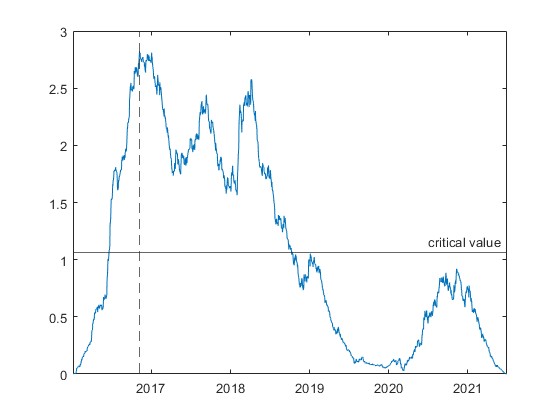
(a) $BS$

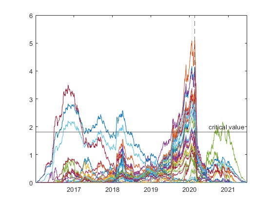
(b) $WBS_{BS}$

Figure 2: Test statistic for all time points using (a) binary segmentation and (b) wild binary segmentation with $50$ random intervals. The dashed line marks the maximal value of the test statistic and therefore the first change point candidate.

Figure 2 illustrates the test statistic of the binary ($BS$) and wild binary segmentation ($WBS_{BS}$) in the first step to find the first change point. $BS$ finds the first break at the end of 2016. Although the test statistic shows signs of a change at the end of 2020, it does not get very large. The test statistic for $WBS_{BS}$ announces a first change point at the beginning of 2020. However, also for the other change points the test statistic exceeds the critical value. Notice that $WBS_{B}S$ includes the test statistic of the binary segmentation.

5 Conclusion

Procedures for the detection of multiple change points for copula-based dependence measures have been analyzed. Focusing on the binary segmentation, consistency results for the amount as well as the location of change points are provided. Additionally, a consistency result for a computationally more efficient information criterion is given. In order to show that the procedures perform well in finite samples, a Monte Carlo simulation is conducted. To generate data, a factor copula with piecewise constant, group specific factor loadings is used. A binary segmentation and two wild binary segmentation algorithms are implemented in order to detect changes in Spearman’s $\rho$. The proposed procedures are then applied on daily return data of companies, included in the EURO STOXX 50 index, to study change points in Spearman’s $\rho$ covering the recent COVID-19 pandemic. The wild binary segmentation algorithms find change points in the dependencies, among others, at the beginning as well as at the second wave of the COVID-19 pandemic.

One interesting avenue for future research could be a more detailed investigation of the information criterion of Remark 2 to find a suitable penalty term leading to a more time efficient procedure for finding multiple change points. The consistency results in this article might provide the foundation of this method. Moreover, checking for breaks in the marginals [using, e.g. Galeano and Tsay, (2009) or Wied et al., 2012a ] in conjunction with a segmentation algorithm to estimate the marginals between the detected changes, could be another interesting question.

Appendix A Proofs

A.1 Proof of Proposition 1

Proof. Proposition 1 follows from Lemma A.1 and A.2 below, in conjunction with the proof of Galeano and Wied, (2017, Theorem 1).

Lemma A.1

For any given interval $[a,b]\subseteq[0,1]$,

$$\textnormal{$\operatorname*{\textsf{sup}}\limits_{z\,\in\,[a,b]}$}\left|\frac{\hat{M}(a,b;z)}{\sqrt{\lfloor bT\rfloor-\lfloor aT\rfloor}}-M(a,b;z)\right|=O_{p}(1/\sqrt{T}).$$

Proof of Lemma A.1. Consider

$$\frac{\hat{M}(a,b;z)}{\sqrt{\lfloor bT\rfloor-\lfloor aT\rfloor}}=\sqrt{\sum_{g\,=\,1}^{G}\sum_{l\,=\,1}^{H}\left[\frac{1}{\displaystyle{|\mathcal{G}_{g}|\choose 2}}\sum\limits_{\begin{subarray}{c}1\leq i<j\leq n\\ i,j\,\in\,\mathcal{G}_{g}\end{subarray}}\frac{\lfloor zT\rfloor-\lfloor aT\rfloor}{\lfloor bT\rfloor-\lfloor aT\rfloor}(\hat{m}_{i,j,l}^{\lfloor zT\rfloor+1:\lfloor bT\rfloor}-\hat{m}_{i,j,l}^{\lfloor aT\rfloor+1:\lfloor bT\rfloor})\right]^{2}},$$

fix an arbitrary pair $(i,j)\in\mathcal{G}_{g},1\leq i<j\leq n$, for some $g\in\{1,\dots,G\}$. Next, choose some $l\in\{1,\dots,H\}$ and define for any given interval $[a,b]\subseteq[0,1]$ the unfeasible dependence measure

$$\tilde{m}_{i,j,l}^{\lfloor aT\rfloor+1:\lfloor bT\rfloor}=\frac{1}{\lfloor bT\rfloor-\lfloor aT\rfloor}\sum_{t\,=\,\lfloor aT\rfloor+1}^{\lfloor bT\rfloor}h_{l}(U_{i,t},U_{j,t}).$$ (A.1)

Note that, by the triangle inequality in conjunction with Assumptions C, one gets

$$\begin{split}|\hat{m}_{i,j,l}^{\lfloor aT\rfloor+1:\lfloor bT\rfloor}-\tilde{m}_{i,j,l}^{\lfloor aT\rfloor+1:\lfloor bT\rfloor}|\leq&\,\frac{c_{0}}{\lfloor bT\rfloor-\lfloor aT\rfloor}\sum_{t\,=\,\lfloor aT\rfloor+1}^{\lfloor bT\rfloor}\sum_{k\,\in\,\{i,j\}}|\hat{U}_{k,t}^{\lfloor aT\rfloor+1:\lfloor bT\rfloor}-U_{k,t}|\\ =&\,\frac{c_{0}}{\lfloor bT\rfloor-\lfloor aT\rfloor}\sum_{t\,=\,\lfloor aT\rfloor+1}^{\lfloor bT\rfloor}\frac{1}{\sqrt{T}}\sum_{k\,\in\,\{i,j\}}|\hat{\mathbb{F}}_{k}(a,b,\eta_{k,t})|\end{split}$$ (A.2)

where

$$\hat{\mathbb{F}}_{i}(a,b,x_{i})=\hat{\mathbb{F}}(a,b,\bm{x}^{i}),\;\;\bm{x}^{i}=(\infty,\dots,\infty,x_{i},\infty,\dots,\infty)$$

for $i\in\{1,\dots,n\}$, with $\hat{\mathbb{F}}(a,b,\bm{x})=\sqrt{T}(\hat{F}^{\lfloor aT\rfloor+1:\lfloor bT\rfloor}-\textnormal{{F}})(\bm{x})$ for $\bm{x}\in\mathbb{R}^{n}$ and $(a,b)\in\Delta$, with $\Delta=\Delta_{0,1}$, where $\Delta_{a,b}=\{(\alpha,\beta)\in[a,b]^{2}:0\leq a\leq b\leq 1\}$ and

$$\hat{F}^{\lfloor aT\rfloor+1:\lfloor bT\rfloor}(\bm{x})=\frac{1}{\lfloor bT\rfloor-\lfloor aT\rfloor}\sum_{t=\lfloor aT\rfloor+1}^{\lfloor bT\rfloor}1\{\hat{\bm{\eta}}_{t}\leq\bm{x}\}.$$

Now, by Assumption A, $\operatorname*{\textsf{max}}_{k\,\in\,\{i,j\}}\operatorname*{\textsf{sup}}_{(a,b,x)\,\in\,\Delta\times\mathbb{R}}\,|\hat{\mathbb{F}}_{k}(a,b,x)|=O_{p}(1)$. Hence, by Eq. (A.2), $\operatorname*{\textsf{sup}}_{(a,b)\,\in\,\Delta}|\hat{m}_{i,j}^{\lfloor aT\rfloor+1:\lfloor bT\rfloor}-\tilde{m}_{i,j}^{\lfloor aT\rfloor+1:\lfloor bT\rfloor}|=O_{p}(1/\sqrt{T}).$ Next, assume, for brevity, two $\ell^{0}=2$ break points $0\eqqcolon z_{0}^{0}<z_{1}^{0}<z_{2}^{0}<z_{3}^{0}\coloneqq 1$, $n=2$, and $H=1$; i.e., $p=1$. Then either 1. $a\leq z_{1}^{0}<z_{2}^{0}\leq b$, 2. $z_{2}^{0}\leq a$, 3. $z_{1}^{0}\leq a<z_{2}^{0}\leq b$, 4. $z_{1}^{0}\leq a<b\leq z_{2}^{0}$, 5. $a\leq z_{1}^{0}<b\leq z_{2}^{0}$, or 6. $z_{1}^{0}\geq b$. Hence,

$$\begin{split}\int_{a}^{z}g(t)\,\textsf{d}t=\,&1\{a\leq z_{1}^{0}<z_{2}^{0}\leq z\}[(z_{1}^{0}-a)\gamma_{0}^{0}+(z_{2}^{0}-z_{1}^{0})\gamma_{1}^{0}+(z-z_{2}^{0})\gamma_{2}^{0}]\\ \,&+1\{a\leq z_{1}^{0}<z\leq z_{2}^{0}\}[(z_{1}^{0}-a)\gamma_{0}^{0}+(z-z_{1}^{0})\gamma_{1}^{0}]\\ \,&+1\{z_{1}^{0}\leq a<z_{2}^{0}\leq z\}[(z_{2}^{0}-a)\gamma_{1}^{0}+(z-z_{2}^{0})\gamma_{2}^{0}]\\ \,&+(b-a)[1\{z_{1}^{0}\geq z\}\gamma_{0}^{0}+1\{z_{1}^{0}\leq a<z\leq z_{2}^{0}\}\gamma_{1}^{0}+1\{z_{2}^{0}\leq a\}\gamma_{2}^{0}].\end{split}$$ (A.3)

Now, consider

$$\begin{split}(\lfloor zT\rfloor-\lfloor aT\rfloor)&\tilde{m}_{i,j}^{\lfloor aT\rfloor+1:\lfloor zT\rfloor}\\ =\,&1\{a\leq z_{1}^{0}<z_{2}^{0}\leq z\}\bigg{[}(\lfloor z_{1}^{0}T\rfloor-\lfloor aT\rfloor)\tilde{m}_{i,j}^{\lfloor aT\rfloor+1:\lfloor z_{1}^{0}T\rfloor}\\ \,&\hskip 99.58464pt+(\lfloor z_{2}^{0}T\rfloor-\lfloor z_{1}^{0}T\rfloor)\tilde{m}_{i,j}^{\lfloor z_{1}^{0}T\rfloor+1:\lfloor z_{2}^{0}T\rfloor}\\ \,&\hskip 99.58464pt+(\lfloor zT\rfloor-\lfloor z_{2}^{0}T\rfloor)\tilde{m}_{i,j}^{\lfloor z_{2}^{0}T\rfloor+1:\lfloor zT\rfloor}\bigg{]}\\ \,&+1\{a\leq z_{1}^{0}<z\leq z_{2}^{0}\}\bigg{[}(\lfloor z_{1}^{0}T\rfloor-\lfloor aT\rfloor)\tilde{m}_{i,j}^{\lfloor aT\rfloor+1:\lfloor z_{1}^{0}T\rfloor}\\ \,&\hskip 99.58464pt+(\lfloor zT\rfloor-\lfloor z_{1}^{0}T\rfloor)\tilde{m}_{i,j}^{\lfloor z_{1}^{0}T\rfloor+1:\lfloor zT\rfloor}\bigg{]}\\ \,&+1\{z_{1}^{0}\leq a<z_{2}^{0}\leq z\}\bigg{[}(\lfloor z_{2}^{0}T\rfloor-\lfloor aT\rfloor)\tilde{m}_{i,j}^{\lfloor aT\rfloor+1:\lfloor z_{2}^{0}T\rfloor}\\ \,&\hskip 99.58464pt+(\lfloor zT\rfloor-\lfloor z_{2}^{0}T\rfloor)\tilde{m}_{i,j}^{\lfloor z_{2}^{0}T\rfloor+1:\lfloor zT\rfloor}\bigg{]}\\ \,&+(1\{z_{1}^{0}\geq z\}+1\{z_{1}^{0}\leq a<z\leq z_{2}^{0}\}+1\{z_{2}^{0}\leq a\})\tilde{m}_{i,j}^{\lfloor aT\rfloor+1:\lfloor zT\rfloor}.\end{split}$$ (A.4)

Next, introduce the unfeasible sequential empirical copula process

$$\tilde{\mathbb{B}}_{i,j,t}(a,b,u,v)=\frac{1}{\sqrt{\lfloor bT\rfloor-\lfloor aT\rfloor}}\sum_{t\,=\,\lfloor aT\rfloor}^{\lfloor bT\rfloor}(1\{U_{i,t}\leq u,U_{j,t}\leq v\}-\textsf{C}_{i,j,t}(u,v)).$$

By part (A1) of Assumption A, one has $\textsf{C}_{i,j,t}=\textsf{C}_{i,j,k}$ for all $\lfloor aT\rfloor\leq t\leq\lfloor bT\rfloor$ and thus $\tilde{\mathbb{B}}_{i,j,t}(\alpha,\beta,u,v)=\tilde{\mathbb{B}}_{i,j,k}(\alpha,\beta,u,v)$ for any $(\alpha,\beta)\in\Delta_{a,b}$, $[a,b]\subseteq[z_{k}^{0},z_{k+1}^{0}]$, $k\in\{0,1,2\}$, and $m_{i,j,t}=\gamma_{k}^{0}=\int_{[0,1]^{2}}h(u,v)\,\textsf{d}\textsf{C}_{i,j,k}(u,v).$ Moreover, by Fermanian et al., (2004, Theorem 6), one gets

$$\sqrt{T}(\tilde{m}_{i,j}^{\lfloor\alpha T\rfloor+1:\lfloor\beta T\rfloor}-m_{i,j,k})=\int_{[0,1]^{2}}\tilde{\mathbb{B}}_{i,j,k}(\alpha,\beta,u,v)\,\textsf{d}h(u,v)+O(1/\sqrt{T}).$$

Since, by Assumption D, $\tilde{\mathbb{C}}_{i,j,k}$ converges weakly for any $k\in\{1,\dots,\ell\}$ on $\Delta_{a,b}\times[0,1]^{2}$ to a tight Gaussian process [see also Bücher and Kojadinovic, (2016)], the claim follows. ∎

Lemma A.2

Define $\hat{z}_{a,b}=\operatorname*{\textsf{arg\,max}}\limits_{z\in[a,b]}\hat{M}(a,b;z)$. For any $[a,b]\subseteq[0,1]$, the change point estimator $\hat{z}_{a,b}$ is consistent for the dominating change point in $[a,b]$ defined as $z_{a,b}^{\star}\coloneqq\operatorname*{\textsf{arg\,max}}\limits_{z\,\in\,[a,b]}M(a,b;z)$.

A.2 Proof of Proposition 2

Proof. The proof follows from part Lemma B.1 and part (1) of Lemma B.2 below.

Lemma B.1

If there is no break in $[z_{k}^{0},z_{k+1}^{0}]$, $k\in\{0,1,\dots,\ell^{0}\}$, then

$$\operatorname*{\textsf{max}}\limits_{k\,\in\,\{0,1,\dots,\ell^{0}\}}\operatorname*{\textsf{sup}}\limits_{z\,\in\,[z_{k}^{0},z_{k+1}^{0}]}\hat{M}_{T}(z_{k}^{0},z_{k+1}^{0};z)\stackrel{{\scriptstyle d}}{{\longrightarrow}}\operatorname*{\textsf{max}}\limits_{k\,\in\,\{0,1,\dots,\ell^{0}\}}\operatorname*{\textsf{sup}}\limits_{z\,\in\,[z_{k}^{0},z_{k+1}^{0}]}\mathbb{M}(z_{k}^{0},z_{k+1}^{0};z).$$

Proof of Lemma B.1. Set $\hat{M}_{k}(z)\coloneqq\hat{M}(z_{k}^{0},z_{k+1}^{0};z)$. Now, for some $k\in\{0,1,\dots,\ell^{0}\}$, $l\in\{1,\dots,H\}$, $g\in\{1,\dots,G\}$, and any pair $(i,j)\in\mathcal{G}_{g}$, $i\neq j$, one has

$$\begin{split}\hat{m}_{i,j,l}^{\lfloor z_{k}^{0}T\rfloor+1:\lfloor zT\rfloor}-&\hat{m}_{i,j,l}^{\lfloor z_{k}^{0}T\rfloor+1:\lfloor z_{k+1}^{0}T\rfloor}\\ \,&=\int_{[0,1]^{2}}(\hat{C}_{i,j}^{\lfloor z_{k}^{0}T\rfloor+1:\lfloor zT\rfloor}-\hat{C}_{i,j}^{\lfloor z_{k}^{0}T\rfloor+1:\lfloor z_{k+1}^{0}T\rfloor})(u,v)\,\textsf{d}h_{l}(u,v)+O_{p}(1/T),\end{split}$$ (A.5)

using Fermanian et al., (2004); see also Berghaus et al., (2017). Moreover, consider

$$\begin{split}\hat{\mathbb{D}}_{k}(z,\bm{u})\coloneqq\,&\frac{\lfloor zT\rfloor-\lfloor z_{k}^{0}T\rfloor}{\sqrt{\lfloor z_{k+1}^{0}T\rfloor-\lfloor z_{k}^{0}T\rfloor}}(\hat{C}^{\lfloor z_{k}^{0}T\rfloor+1:\lfloor zT\rfloor}-\hat{C}^{\lfloor z_{k}^{0}T\rfloor+1:\lfloor z_{k+1}^{0}T\rfloor})(\bm{u})\\ =\,&\hat{\mathbb{C}}_{k}(z,\bm{u})-\varphi_{k}(z)\hat{\mathbb{C}}_{k}(z_{k+1}^{0},\bm{u}),\end{split}$$ (A.6)

where

$$\hat{\mathbb{C}}_{k}(z,\bm{u})\coloneqq\frac{1}{\sqrt{\lfloor z_{k+1}^{0}T\rfloor-\lfloor z_{k}^{0}T\rfloor}}\sum_{t\,=\,\lfloor z_{k}^{0}T\rfloor+1}^{\lfloor zT\rfloor}(1\{\hat{\bm{U}}_{t}^{\lfloor z_{k}^{0}T\rfloor+1:\lfloor zT\rfloor}\leq\bm{u}\}-\textsf{C}_{k+1}(\bm{u}))$$ (A.7)

for $z\in[z_{k}^{0},z_{k+1}^{0}]$. We can deduce from Bücher and Kojadinovic, (2016) and Nasri et al., (2022) in conjunction with the continuous mapping theorem, that $\hat{\mathbb{C}}_{k}\rightsquigarrow\mathbb{C}_{k}$ in $\ell^{\infty}([z_{k}^{0},z_{k+1}^{0}]\times[0,1]^{n})$. Hence, $\hat{\mathbb{D}}_{k}\rightsquigarrow\mathbb{D}_{k}$ in $\ell^{\infty}([z_{k}^{0},z_{k+1}^{0}]\times[0,1]^{n})$, where $\mathbb{D}_{k}(z,\bm{u})=\mathbb{C}_{k}(z,\bm{u})-\varphi_{k}(z)\mathbb{C}_{k}(z_{k+1},\bm{u}).$ Therefore,

$$\begin{split}\frac{\lfloor zT\rfloor-\lfloor z_{k}^{0}T\rfloor}{\sqrt{\lfloor z_{k+1}^{0}T\rfloor-\lfloor z_{k}^{0}T\rfloor}}(\hat{m}_{i,j,l}^{\lfloor z_{k}^{0}T\rfloor+1:\lfloor zT\rfloor}-&\hat{m}_{i,j,l}^{\lfloor z_{k}^{0}T\rfloor+1:\lfloor z_{k+1}^{0}T\rfloor})\\ \,&\rightsquigarrow\int_{[0,1]^{2}}\mathbb{D}_{k,i,j}(z,u,v)\,\textsf{d}h_{l}(u,v),\end{split}$$ (A.8)

so that $\operatorname*{\textsf{sup}}\limits_{z\,\in\,[z_{k}^{0},z_{k+1}^{0}]}\hat{M}_{k}(z)\stackrel{{\scriptstyle d}}{{\rightarrow}}\operatorname*{\textsf{sup}}\limits_{z\,\in\,[z_{k}^{0},z_{k+1}^{0}]}\mathbb{M}_{k}(z).$ Since $\{\mathbb{M}_{k}(z)\}_{k\,=\,0}^{\ell^{0}}$ are independent and Gaussian, the claim follows by the continuous mapping theorem.

Lemma B.2

.

1. If there is no break in $[z_{k}^{0},z_{k+1}^{0}]$ for all $k\in\{0,1,\dots,\ell^{0}\}$, then

   $$\operatorname*{\textsf{max}}\limits_{0\,\leq\,k\,\leq\,\ell}\left|\operatorname*{\textsf{sup}}\limits_{z\in[z_{k}^{0},z_{k+1}^{0}]}\hat{M}(z_{k}^{0},z_{k+1}^{0};z)-\operatorname*{\textsf{sup}}\limits_{z\in[\hat{z}_{k},\hat{z}_{k+1}]}\hat{M}(\hat{z}_{k},\hat{z}_{k+1};z)\right|=O_{p}(1/\sqrt{T}).$$

2. If there is at least one break in $[z_{k}^{0},z_{k+1}^{0}]$ for at least one $k\in\{0,1,\dots,\ell\}$, then

   $$\operatorname*{\textsf{max}}\limits_{0\,\leq\,k\,\leq\,\ell}\left|\operatorname*{\textsf{sup}}\limits_{z\in[z_{k},z_{k+1}]}\hat{M}(z_{k}^{0},z_{k+1}^{0};z)-\operatorname*{\textsf{sup}}\limits_{z\in[\hat{z}_{k},\hat{z}_{k+1}]}\hat{M}(\hat{z}_{k},\hat{z}_{k+1};z)\right|=O_{p}(1).$$

Proof of Lemma B.2. We assume, w.l.o.g., that $\ell^{0}=1$; i.e., $0\eqqcolon z_{0}^{0}<z_{1}^{0}<z_{2}^{0}\coloneqq 1$. Set $\hat{M}_{1}(z)\coloneqq\hat{M}(0,z_{1}^{0};z)$, $\hat{M}_{\hat{z}_{1}}(z)\coloneqq\hat{M}(0,\hat{z}_{1};z)$ and define

$$Z_{1}(\hat{z}_{1})\coloneqq\operatorname*{\textsf{sup}}\limits_{z\,\in\,[0,z_{1}^{0}]}\hat{M}_{1}(z)-\operatorname*{\textsf{sup}}\limits_{z\,\in\,[0,\hat{z}_{1}]}\hat{M}_{\hat{z}_{1}}(z).$$

Next, define $D_{T}\coloneqq\{z:z\in[0,1],\,|z-z_{1}|\leq c_{0}/T\}$ for some $c_{0}\in(0,\infty)$ and note that for any $\delta>0$ and $\epsilon>0$

$$\begin{split}\textsf{P}(|Z_{1}(\hat{z}_{1})|>\delta)\leq\,&\textsf{P}(\hat{z}_{1}\notin D_{T})+\textsf{P}(\{|Z_{1}(\hat{z}_{1})|>\delta\}\,\cap\,\{\hat{z}_{1}\in D_{T}\})\\ \leq\,&\epsilon+\textsf{P}\bigg{(}\operatorname*{\textsf{sup}}\limits_{\zeta\,\in\,D_{T}}|Z_{1}(\zeta)|>\delta\bigg{)}.\end{split}$$ (A.9)

Hence, it suffices to show that $|Z_{1}(\zeta)|=o_{p}(1)$ uniformly in $\zeta\in D_{T}$. To see this, note that

$$\begin{split}\left|\operatorname*{\textsf{sup}}\limits_{z\,\in\,[0,z_{1}]}\hat{M}_{1}(z)-\operatorname*{\textsf{sup}}\limits_{z\,\in\,[0,\zeta]}\hat{M}_{\zeta}(z)\right|\leq\,&\operatorname*{\textsf{sup}}\limits_{z\,\in\,[0,z_{1}]}\left|\hat{M}_{1}(z)-\hat{M}_{\zeta}(z)\right|\\ \,&+\left|\operatorname*{\textsf{sup}}\limits_{z\,\in\,[0,z_{1}]}\hat{M}_{\zeta}(z)-\operatorname*{\textsf{sup}}\limits_{z\,\in\,[0,\zeta]}\hat{M}_{\zeta}(z)\right|\coloneqq A(\zeta)+B(\zeta),\end{split}$$ (A.10)

say. Begin with $A(\zeta)$. Suppose, w.l.o.g., that $\zeta>z_{1}$. Consider

$$\begin{split}\left|\hat{M}_{1}(z)-\hat{M}_{\zeta}(z)\right|=\,&\frac{\lfloor zT\rfloor}{\sqrt{\lfloor\zeta T\rfloor}}\left|\sqrt{\frac{\lfloor\zeta T\rfloor}{\lfloor z_{1}T\rfloor}}\lVert\hat{\bm{m}}^{1:\lfloor zT\rfloor}-\hat{\bm{m}}^{1:\lfloor z_{1}T\rfloor}\rVert_{2}-\lVert\hat{\bm{m}}^{1:\lfloor zT\rfloor}-\hat{\bm{m}}^{1:\lfloor\zeta T\rfloor}\rVert_{2}\right|\\ \leq\,&\sqrt{1-\frac{\lfloor z_{1}T\rfloor}{\lfloor\zeta T\rfloor}}\hat{M}_{1}(z)+\frac{\lfloor zT\rfloor}{\sqrt{\lfloor\zeta T\rfloor}}A_{1}(\zeta),\end{split}$$ (A.11)

where $A_{1}(\zeta)\coloneqq\lVert\hat{\bm{m}}^{1:\lfloor\zeta T\rfloor}-\hat{\bm{m}}^{1:\lfloor z_{1}T\rfloor}\rVert_{2}$; for the inequality, we expanded the term in absolute values on the right-hand side of the equality with $\lVert\hat{\bm{m}}^{1:\lfloor zT\rfloor}-\hat{\bm{m}}^{1:\lfloor z_{1}T\rfloor}\rVert_{2}$, we used the (reverse) triangle inequality and $\sqrt{u}-\sqrt{v}\leq\sqrt{u-v}$ for $u\geq v\geq 0$. It follows that $\operatorname*{\textsf{sup}}\limits_{z\,\in\,[0,z_{1}]}\hat{M}_{1}(z)=O_{p}(1)$ if there is no break in $[0,z_{1}]$ or $\operatorname*{\textsf{sup}}\limits_{z\,\in\,[0,z_{1}]}\hat{M}_{1}(z)/\sqrt{T}=O_{p}(1)$ if there is at least one break in $[0,z_{1}]$. Turning to $A_{1}(\zeta)$, the triangle inequality and $\lVert\bm{v}\rVert_{2}\leq n\operatorname*{\textsf{max}}_{1\leq i\leq n}|v_{i}|$ for any $\bm{v}\in\mathbb{R}^{n}$ yields

$$\begin{split}A_{1}(\zeta)\leq\,&p\operatorname*{\textsf{max}}_{1\,\leq\,l\,\leq\,H}\operatorname*{\textsf{max}}_{1\,\leq\,g\,\leq\,G}\operatorname*{\textsf{max}}\limits_{(i,j)\,\in\,\mathcal{G}_{g}}\bigg{[}\frac{1}{\lfloor\zeta T\rfloor}\sum_{t\,=\,\lfloor z_{1}T\rfloor}^{\lfloor\zeta T\rfloor}\left|h_{l}(\hat{U}_{i,t}^{1:\lfloor\zeta T\rfloor},\hat{U}_{j,t}^{1:\lfloor\zeta T\rfloor})\right|\\ \,&\hskip 7.11317pt+\left(\frac{\lfloor\zeta T\rfloor}{\lfloor z_{1}T\rfloor}-1\right)\frac{1}{\lfloor z_{1}T\rfloor}\sum_{t\,=\,1}^{\lfloor z_{1}T\rfloor}\left|h_{l}(\hat{U}_{i,t}^{1:\lfloor\zeta T\rfloor},\hat{U}_{j,t}^{1:\lfloor\zeta T\rfloor})\right|\\ \,&\hskip 7.11317pt+\frac{1}{\lfloor z_{1}T\rfloor}\sum_{t\,=\,1}^{\lfloor z_{1}T\rfloor}\left|h_{l}(\hat{U}_{i,t}^{1:\lfloor\zeta T\rfloor},\hat{U}_{j,t}^{1:\lfloor\zeta T\rfloor})-h_{l}(\hat{U}_{i,t}^{1:\lfloor z_{1}T\rfloor},\hat{U}_{j,t}^{1:\lfloor z_{1}T\rfloor})\right|\bigg{]}\end{split}$$

say. It follows from assumption C that $\operatorname*{\textsf{max}}_{1\,\leq\,l\,\leq\,H}\operatorname*{\textsf{sup}}\limits_{(u,v)\,\in\,[0,1]^{2}}|h_{l}(u,v)|\leq c_{0}$ for some $c_{0}\in(0,\infty)$. Hence the first to summands on the preceding display are $O(1/T)$ uniformly in $\zeta\in D_{T}$. Turning to the third summand, note that, by Assumption (C2), one gets for some $c_{0}\in(0,\infty)$

$$\begin{split}\frac{1}{\lfloor z_{1}T\rfloor}\sum_{t\,=\,1}^{\lfloor z_{1}T\rfloor}\Big{|}h_{l}(\hat{U}_{i,t}^{1:\lfloor\zeta T\rfloor}&,\hat{U}_{j,t}^{1:\lfloor\zeta T\rfloor})-h_{l}(\hat{U}_{i,t}^{1:\lfloor z_{1}T\rfloor},\hat{U}_{j,t}^{1:\lfloor z_{1}T\rfloor})\Big{|}\\ \,&\leq 2c_{0}\operatorname*{\textsf{max}}\limits_{k\,\in\,\{i,j\}}\operatorname*{\textsf{sup}}_{x\,\in\,\mathbb{R}}\left|\hat{F}_{k}^{1:\lfloor\zeta T\rfloor}(x)-\hat{F}_{k}^{1:\lfloor z_{1}T\rfloor}(x)\right|=O_{p}(1/T).\end{split}$$ (A.12)

Putting the above together yields, uniformly in $\zeta\in D_{T}$, $A(\zeta)=O_{p}(1/\sqrt{T})$ if there is no break and $A(\zeta)=O_{p}(1)$ if there is at least one break in $[0,1]$. Turning to $B(\zeta)$, a simple calculation reveals that

$$B(\zeta)\leq\operatorname*{\textsf{sup}}\limits_{z\,\in\,[z_{1},\zeta]}\left|\hat{M}_{\zeta}(z)-\hat{M}_{\zeta}(z_{1})\right|\leq\operatorname*{\textsf{sup}}\limits_{z\,\in\,[z_{1},\zeta]}\frac{\lfloor zT\rfloor}{\sqrt{\zeta T}}\lVert\hat{\bm{m}}^{1:\lfloor zT\rfloor}-\hat{\bm{m}}^{1:\lfloor z_{1}T\rfloor}\rVert_{2}=O_{p}(1/\sqrt{T}),$$

noting that there is no nontrivial break in $[z_{1},\zeta]$.

A.3 Additional Results for the Information Criterion

Adopting the notation of Remark 2 and using an idea from Andrews, (1999), we introduce the set of selection vectors

$$\mathcal{C}_{L}\coloneqq\left\{\bm{c}=(c_{1},\dots,c_{L})^{\prime}\in\mathbb{R}^{L}\mid c_{j}\in\{0,1\},\,1\leq j\leq L\right\}.$$

Recall from Remark 2 that we define for any $\bm{c}\in\mathcal{C}_{L}$ our break-point ‘information criterion’ as

$$\textsf{IC}_{T}(\bm{c})\coloneqq\hat{S}^{2}(\bm{c})+h(|\bm{c}|_{1})\kappa_{T},$$ (A.13)

where $\hat{S}(\bm{c})\coloneqq\hat{S}(\bm{k}_{c})$, with

$$\begin{split}\hat{S}(\bm{k}_{c})\coloneqq\,&\operatorname*{\textsf{max}}\limits_{1\,\leq\,j\,\leq\,|\bm{c}|_{1}+1}\operatorname*{\textsf{max}}\limits_{k_{c,j-1}\,<\,t\,\leq\,k_{c,j}}\hat{S}(k_{c,j-1},k_{c,j};t)\\ \hat{S}(k_{c,j-1},k_{c,j};t)\coloneqq\,&\frac{t-k_{c,j-1}}{\sqrt{k_{c,j}-k_{c,j-1}}}\lVert\hat{\bm{m}}^{k_{c,j-1}+1:t}-\hat{\bm{m}}^{k_{c,j-1}+1:k_{c,j}}\rVert_{2},\;\;\hat{k}_{0,c}\coloneqq 1,\,\hat{k}_{|\bm{c}|_{1}+1,c}\coloneqq T,\end{split}$$

while $h(\cdot)$ and the penalty $\kappa_{T}$ are defined below.

Assumption IC

a) The function $h:\mathbb{R}_{+}\rightarrow\mathbb{R}_{+}$ is strictly increasing. b) $\kappa_{T}\rightarrow\infty$ and $\kappa_{T}=o(T)$.

Assumption is the same as in Andrews, (1999) and Andrews and Lu, (2001). Finally, we define the estimator $\hat{\bm{c}}$ via

$$\hat{\bm{c}}\coloneqq\operatorname*{arg\,min}_{\bm{c}\,\in\,\mathcal{C}_{L}}\textsf{IC}_{T}(\bm{c}).$$

Our objective here is twofold. Firstly, we want to obtain at least as many break points as to ensure that the corresponding intervals $([\hat{k}_{j-1,c},\hat{k}_{j,c}])_{j\,=\,1}^{|\bm{c}|_{1}+1}$, do not contain further nontrivial break points. If this is indeed the case, then Proposition 2 reveals $\hat{S}(\bm{c})/\sqrt{T}=o_{p}(1)$; on the other hand, if there is at least one nontrivial break in between $([\hat{k}_{j-1,c},\hat{k}_{j,c}])_{j\,=\,1}^{|\bm{c}|_{1}+1}$, then, by Lemma B.2, $\hat{S}(\bm{c})/\sqrt{T}\stackrel{{\scriptstyle p}}{{\rightarrow}}\textsf{const}\in(0,\infty)$. Thus our candidate $\bm{c}\in\mathcal{C}_{L}$ should, with probability approaching one (wp $\rightarrow 1$), satisfy $\bm{c}\in\mathcal{B}_{L}$, where

$$\mathcal{B}_{L}\coloneqq\left\{\bm{c}\in\mathcal{C}_{L}\mid\hat{S}(\bm{c})/\sqrt{T}=o_{p}(1)\right\}.$$

Secondly, provided some $\bm{c}\in\mathcal{B}_{L}$ is chosen, we would like to obtain the most parsimonious set of break points; i.e. $\bm{c}$ should fall wp $\rightarrow 1$ into the set

$$\mathcal{MB}_{L}\coloneqq\left\{\bm{c}\in\mathcal{B}_{L}\mid|\bm{c}|\leq|\bm{c}^{\prime}|,\;\forall\,\bm{c}^{\prime}\in\mathcal{B}_{L}\right\}.$$

We can show that $\hat{\bm{c}}\in\mathcal{MB}_{L}$ wp $\rightarrow 1$, provided $\ell_{0}\leq L$. Since $\mathcal{MB}_{L}=\{\bm{c}_{0}\}$, it follows immediately that $|\hat{\bm{c}}|_{1}\stackrel{{\scriptstyle p}}{{\rightarrow}}\ell^{0}$.

Proposition 4

If $\ell^{0}\leq L$, then $(\hat{\bm{k}}_{\hat{c}}/T,|\hat{\bm{c}}|_{1})\stackrel{{\scriptstyle p}}{{\longrightarrow}}(\bm{z}^{0},\ell^{0})$, where $\bm{z}^{0}\coloneqq(z_{1}^{0},\dots,z_{\ell^{0}}^{0})^{\prime}$; compare assumption A.

Proof. The following mimics the proof in Andrews, (1999). It follows readily that $\hat{S}^{2}(\bm{k})/T=o_{p}(1)$ if there is no break and $\hat{S}^{2}(\bm{k})/T\stackrel{{\scriptstyle p}}{{\rightarrow}}\textsf{const}\in(0,\infty)$, otherwise. By definition of (A.13), one concludes $\hat{\bm{c}}\in\mathcal{B}_{L}$ wp $\rightarrow 1$. If we take $\bm{c}_{1},\bm{c}_{2}\in\mathcal{B}_{L}$ with $\bm{c}_{1}\in\mathcal{MB}_{L}$ and $\bm{c}_{2}\notin\mathcal{MB}_{L}$, then $|\bm{c}_{1}|_{1}\leq|\bm{c}_{2}|_{1}$ and $(h(|\bm{c}_{1}|_{1})-h(|\bm{c}_{2}|_{1}))\kappa_{T}\rightarrow-\infty$. Therefore, $\textsf{IC}_{T}(\bm{c}_{1})\leq\textsf{IC}_{T}(\bm{c}_{2})$ wp $\rightarrow 1$ so that $\hat{\bm{c}}\in\mathcal{MB}_{L}=\{\bm{c}_{0}\}$ wp $\rightarrow 1$.

Appendix B Tables

loadings	0 breaks	1 break		2 breaks			3 breaks
	$[1,T]$	$[1,t_{1}]$	$(t_{1},T]$	$[1,0.4T]$	$(0.4T,0.6T]$	$(0.6T,T]$	$[1,0.3T]$	$(0.3T,0.5T]$	$(0.5T,0.7T]$	$(0.7T,T]$
$\beta_{1,t}$	1	1	0.5	1	0.5	1	0.7	1	0.4	0.7
$\beta_{2,t}$	0.5	0.5	1	0.5	1	0.5	0.7	0.4	1	0.7
$\beta_{3,t}$	1	1	1	1	1	1	0.7	0.7	0.7	0.7
$\beta_{4,t}$	1.5	1.5	0.5	1.5	0.5	1.5	0.7	1.2	0.2	0.7
$\rho_{1}$	0.4469	0.4469	0.2006	0.4469	0.2006	0.4469	0.3074	0.4469	0.1459	0.3074
$\rho_{2}$	0.2006	0.2006	0.4469	0.2006	0.4469	0.2006	0.3074	0.1459	0.4469	0.3074
$\rho_{3}$	0.4469	0.4469	0.4469	0.4469	0.4469	0.4469	0.3074	0.3074	0.3074	0.3074
$\rho_{4}$	0.6132	0.6132	0.2006	0.6132	0.2006	0.6132	0.3074	0.5212	0.0465	0.3074
$\bar{\rho}$	0.4269	0.4269	0.3238	0.4269	0.3238	0.4269	0.3074	0.3554	0.2367	0.3074

Table B.1: loadings from the DGP (7) with $4$ groups in the corresponding interval. $\rho_{i}$ contains the cross-sectional average of Spearman’s $\rho$ in group $i$ averaged over 10000 simulations. $\bar{\rho}$ is the average over $\rho_{i}$

$BS$	0breaks	1break			2breaks	3breaks
		$z_{1}$=0.15	$z_{1}$=0.5	$z_{1}$=0.85	$z_{1}$=0.4	$z_{1}$=0.3
					$z_{2}$=0.6	$z_{2}$=0.5 $z_{3}$=0.7
-3						0.043
-2					0.354	0.013
-1		0.000	0.000	0.037	0.000	0.322
0	0.906	0.600	0.931	0.711	0.558	0.597
1	0.085	0.370	0.068	0.236	0.084	0.024
2	0.008	0.028	0.001	0.016	0.004	0.001
3	0.001	0.002	0.000	0.000	0.000	0.000
$WBS$
-3						0.008
-2					0.013	0.461
-1		0.284	0.000	0.549	0.233	0.430
0	0.902	0.621	0.933	0.404	0.678	0.093
1	0.092	0.086	0.065	0.043	0.075	0.008
2	0.006	0.009	0.002	0.004	0.001	0.000
3	0.000	0.000	0.000	0.000	0.000	0.000
$WBS_{BS}$
-3						0.012
-2					0.016	0.312
-1		0.092	0.000	0.488	0.082	0.517
0	0.907	0.753	0.925	0.443	0.882	0.148
1	0.086	0.143	0.073	0.065	0.076	0.011
2	0.007	0.012	0.002	0.004	0.004	0.000
3	0.000	0.000	0.000	0.000	0.000	0.000

Table B.2: Over- and underestimation frequencies of the amount of true change points $\hat{\ell}-\ell^{0}$ with $\alpha=0.01$ and $T=500$

$BS$	0breaks	1break			2breaks	3breaks
		$z_{1}$=0.15	$z_{1}$=0.5	$z_{1}$=0.85	$z_{1}$=0.4	$z_{1}$=0.3
					$z_{2}$=0.6	$z_{2}$=0.5 $z_{3}$=0.7
-3						0.000
-2					0.004	0.000
-1		0.000	0.000	0.000	0	0.000
0	0.958	0.562	0.974	0.861	0.936	0.968
1	0.039	0.427	0.026	0.137	0.060	0.032
2	0.003	0.011	0.000	0.002	0.000	0.000
3	0.000	0.000	0.000	0.000	0.000	0.000
$WBS$
-3						0.000
-2					0.000	0.005
-1		0.017	0.000	0.058	0.002	0.146
0	0.958	0.864	0.978	0.904	0.972	0.827
1	0.042	0.113	0.021	0.036	0.025	0.022
2	0.000	0.006	0.001	0.002	0.001	0.000
3	0.000	0.000	0.000	0.000	0.000	0.000
$WBS_{BS}$
-3						0.000
-2					0.000	0.000
-1		0.000	0.000	0.000	0.000	0.026
0	0.974	0.743	0.973	0.943	0.979	0.944
1	0.023	0.250	0.027	0.055	0.020	0.030
2	0.003	0.007	0.000	0.002	0.001	0.000
3	0.000	0.000	0.000	0.000	0.000	0.000

Table B.3: Over- and underestimation frequencies of the amount of true change points $\hat{\ell}-\ell^{0}$ with $\alpha=0.0333$ and $T=1500$

$BS$	0breaks	1break			2breaks	3breaks
		$z_{1}$=0.15	$z_{1}$=0.5	$z_{1}$=0.85	$z_{1}$=0.4	$z_{1}$=0.3
					$z_{2}$=0.6	$z_{2}$=0.5 $z_{3}$=0.7
-3						0.000
-2					0.035	0.000
-1		0.000	0.000	0.000	0.000	0.064
0	0.944	0.627	0.959	0.800	0.888	0.896
1	0.055	0.357	0.039	0.196	0.077	0.039
2	0.001	0.015	0.002	0.004	0.000	0.001
3	0.000	0.001	0.000	0.000	0.000	0.000
$WBS$
-3						0.000
-2					0.000	0.108
-1		0.060	0.000	0.139	0.007	0.509
0	0.950	0.837	0.956	0.809	0.945	0.371
1	0.047	0.093	0.042	0.050	0.046	0.012
2	0.003	0.010	0.002	0.002	0.002	0.000
3	0.000	0.000	0.000	0.000	0.000	0.000
$WBS_{BS}$
-3						0.000
-2					0.000	0.021
-1		0.000	0.000	0.019	0.001	0.379
0	0.950	0.825	0.951	0.898	0.943	0.568
1	0.048	0.168	0.044	0.078	0.053	0.032
2	0.002	0.006	0.005	0.005	0.003	0.000
3	0.000	0.001	0.000	0.000	0.000	0.000

Table B.4: Over- and underestimation frequencies of the amount of true change points $\hat{\ell}-\ell^{0}$ for filtered data with $\alpha=0.05$ and $T=1000$

References

• Andrews and Lu, (2001) Andrews, D. W. and Lu, B. (2001). Consistent model and moment selection procedures for gmm estimation with application to dynamic panel data models. Journal of Econometrics, 101:123–164.
• Andrews, (1999) Andrews, D. W. K. (1999). Consistent moment selection procedures for generalized method of moments estimation. Econometrica, 67:543–563.
• Aue et al., (2009) Aue, A., Hörmann, S., Horváth, L., and Reimherr, M. (2009). Break detection in the covariance structure of multivariate time series models. The Annals of Statistics, 37:4046–4087.
• Bai, (1997) Bai, J. (1997). Estimating multiple breaks one at a time. Econometric Theory, 13:315–352.
• Bai and Perron, (1998) Bai, J. and Perron, P. (1998). Estimating and testing linear models with multiple structural changes. Econometrica, 66:47–78.
• Barassi et al., (2020) Barassi, M., Horváth, L., and Zhao, Y. (2020). Change‐point detection in the conditional correlation structure of multivariate volatility models. Journal of Business & Economic Statistics, 38:340–349.
• Berghaus et al., (2017) Berghaus, B., Bücher, A., and Volgushev, S. (2017). Weak convergence of the empirical copula process with respect to weighted metrics. Bernoulli, 23:743–772.
• Bücher and Kojadinovic, (2016) Bücher, A. and Kojadinovic, I. (2016). A dependent multiplier bootstrap for the sequential empirical copula process under strong mixing. Bernoulli, 22:927–968.
• Bücher et al., (2014) Bücher, A., Kojadinovic, I., Rohmer, T., and Segers, J. (2014). Detecting changes in cross-sectional dependence in multivariate time series. Journal of Multivariate Analysis, 132:111–128.
• Chen and Fan, (2006) Chen, X. and Fan, Y. (2006). Estimation and model selection of semiparametric copula-based multivariate dynamic models under copula misspecification. Journal of Econometrics, 135:125–154.
• Creal and Tsay, (2015) Creal, D. D. and Tsay, R. S. (2015). High dimensional dynamic stochastic copula models. Journal of Econometrics, 189:335–345.
• Fermanian et al., (2004) Fermanian, J.-D., Radulovic, D., and Wegkamp, M. (2004). Weak convergence of empirical copula processes. Bernoulli, 10:847–860.
• Francq and Zakoïan, (2004) Francq, C. and Zakoïan, J.-M. (2004). Maximum likelihood estimation of pure GARCH and ARMA-GARCH processes. Bernoulli, 10:605–637.
• Fryzlewicz, (2014) Fryzlewicz, P. (2014). Wild binary segmentation for multiple change-point detection. The Annals of Statistics, 42:2243–2281.
• Fryzlewicz, (2020) Fryzlewicz, P. (2020). Detecting possibly frequent change-points: Wild binary segmentation 2 and steepest-drop model selection. Journal of the Korean Statistical Society, 49:1027–1070.
• Galeano and Tsay, (2009) Galeano, P. and Tsay, R. S. (2009). Shifts in individual parameters of a GARCH model. Journal of Financial Econometrics, 8:122–153.
• Galeano and Wied, (2014) Galeano, P. and Wied, D. (2014). Multiple break detection in the correlation structure of random variables. Computational Statistics & Data Analysis, 76:262–282.
• Galeano and Wied, (2017) Galeano, P. and Wied, D. (2017). Dating multiple change points in the correlation matrix. Test, 26:331–352.
• Gombay and Horváth, (1999) Gombay, E. and Horváth, L. (1999). Change-points and bootstrap. Environmetrics, 10:725–736.
• Kojadinovic et al., (2016) Kojadinovic, I., Quessy, J.-F., and Rohmer, T. (2016). Testing the constancy of spearman’s rho in multivariate time series. Annals of the Institute of Statistical Mathematics, 68:929–954.
• Krupskii and Joe, (2013) Krupskii, P. and Joe, H. (2013). Factor copula models for multivariate data. Journal of Multivariate Analysis, 120:85–101.
• Manner et al., (2019) Manner, H., Stark, F., and Wied, D. (2019). Testing for structural breaks in factor copula models. Journal of Econometrics, 208:324–345.
• Markowitz, (1952) Markowitz, H. (1952). Portfolio selection. The Journal of Finance, 7:77–91.
• Nasri et al., (2022) Nasri, B. R., Rémillard, B. N., and Bahraoui, T. (2022). Change-point problems for multivariate time series using pseudo-observations. Journal of Multivariate Analysis, 187:104857.
• Nelsen, (2006) Nelsen, R. B. (2006). An introduction to copulas. Springer, New York.
• Oh and Patton, (2013) Oh, D. H. and Patton, A. J. (2013). Simulated method of moments estimation for copula-based multivariate models. Journal of the American Statistical Association, 108:689–700.
• Oh and Patton, (2017) Oh, D. H. and Patton, A. J. (2017). Modeling dependence in high dimensions with factor copulas. Journal of Business & Economic Statistics, 35:139–154.
• Oh and Patton, (2021) Oh, D. H. and Patton, A. J. (2021). Dynamic factor copula models with estimated cluster assignments. FEDS Working Paper No. 2021-029R1.
• Okui and Wang, (2021) Okui, R. and Wang, W. (2021). Heterogeneous structural breaks in panel data models. Journal of Econometrics, 220:447–473.
• Opschoor et al., (2021) Opschoor, A., Lucas, A., Barra, I., and van Dijk, D. (2021). Closed-form multi-factor copula models with observation-driven dynamic factor loadings. Journal of Business & Economic Statistics, 39:1066–1079.
• Patton, (2006) Patton, A. J. (2006). Modelling asymmetric exchange rate dependence. International Economic Review, 47:527–556.
• Penzer et al., (2012) Penzer, J., Schmid, F., and Schmidt, R. (2012). Measuring large comovements in financial markets. Quantitative Finance, 12:1037–1049.
• Quessy, (2009) Quessy, J.-F. (2009). Theoretical efficiency comparisons of independence tests based on multivariate versions of spearman’s rho. Metrika, 70:315–338.
• Schmid and Schmidt, (2007) Schmid, F. and Schmidt, R. (2007). Multivariate conditional versions of spearman’s rho and related measures of tail dependence. Journal of Multivariate Analysis, 98:1123–1140.
• Segers, (2012) Segers, J. (2012). Asymptotics of empirical copula processes under non-restrictive smoothness assumptions. Bernoulli, 18:764–782.
• Stark and Otto, (2022) Stark, F. and Otto, S. (2022). Testing and dating structural changes in copula-based dependence measures. Journal of Applied Statistics, 49:1121–1139.
• van der Vaart and Wellner, (1996) van der Vaart, A. W. and Wellner, J. A. (1996). Weak convergence and empirical processes. Springer, New York.
• Venkatraman, (1992) Venkatraman, E. S. (1992). Consistency results in multiple change-point problems. PhD thesis, Stanford University.
• Vostrikova, (1981) Vostrikova, L. (1981). Detecting ‘disorder’ in multidimensional random processes. Sov. Dokl. Math., 24:55–59.
• Wang et al., (2020) Wang, W., He, X., and Zhu, Z. (2020). Statistical inference for multiple change-point models. Scandinavian Journal of Statistics, 47:1149–1170.
• (41) Wied, D., Arnold, M., Bissantz, N., and Ziggel, D. (2012a). A new fluctuation test for constant variances with applications to finance. Metrika, 75:1111–1127.
• Wied et al., (2014) Wied, D., Dehling, H., van Kampen, M., and Vogel, D. (2014). A fluctuation test for constant spearman’s rho with nuisance-free limit distribution. Computational Statistics & Data Analysis, 76:723–736.
• (43) Wied, D., Krämer, W., and Dehling, H. (2012b). Testing for a change in correlation at an unknown point in time using an extended functional delta method. Econometric Theory, 28:570–589.