Spatial Entropy as an Inductive Bias for Vision Transformers

Abstract

Recent work on Vision Transformers (VTs) showed that introducing a local inductive bias in the VT architecture helps reducing the number of samples necessary for training. However, the architecture modifications lead to a loss of generality of the Transformer backbone, partially contradicting the push towards the development of uniform architectures, shared, e.g., by both the Computer Vision and the Natural Language Processing areas. In this work, we propose a different and complementary direction, in which a local bias is introduced using an auxiliary self-supervised task, performed jointly with standard supervised training. Specifically, we exploit the observation that the attention maps of VTs, when trained with self-supervision, can contain a semantic segmentation structure which does not spontaneously emerge when training is supervised. Thus, we explicitly encourage the emergence of this spatial clustering as a form of training regularization. In more detail, we exploit the assumption that, in a given image, objects usually correspond to few connected regions, and we propose a spatial formulation of the information entropy to quantify this object-based inductive bias. By minimizing the proposed spatial entropy, we include an additional self-supervised signal during training. Using extensive experiments, we show that the proposed regularization leads to equivalent or better results than other VT proposals which include a local bias by changing the basic Transformer architecture, and it

can drastically boost the VT final accuracy when using small-medium training sets. The code is available at https://github.com/helia95/SAR.

1 Introduction

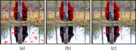
Figure 1: ViT attention maps obtained using the [CLS] token query and thresholded to keep $60\%$ of the mass following (Caron ., 2021). (a) Standard supervised learning. (b) DINO. (c) Training using SAR. In (c), the two largest connected components correspond to the main object (a bear, occluded by a tree), while the third and the fourth largest connected components correspond to the specular reflection of the bear into the river.

Vision Transformers (VTs) are increasingly emerging as the dominant Computer Vision architecture, alternative to standard Convolutional Neural Networks (CNNs). VTs are inspired by the Transformer network (Vaswani ., 2017), which is the de facto standard in Natural Language Processing (NLP) (Devlin ., 2019; Radford  Narasimhan, 2018) and it is based on multi-head attention layers transforming the input tokens (e.g., language words) into a set of final embedding tokens. Dosovitskiy . (2021) proposed an analogous processing paradigm, called ViT, where word tokens are replaced by image patches, and self-attention layers are used to model global pairwise dependencies over all the input tokens. As a consequence, differently from CNNs, where the convolutional kernels have a spatially limited receptive field, ViT has a dynamic receptive field, which is given by its attention maps (Naseer ., 2021). However, ViT heavily relies on huge training datasets (e.g., JFT-300M (Dosovitskiy ., 2021), a proprietary dataset of 303 million images), and underperforms CNNs when trained on ImageNet-1K ($\sim$ 1.3 million images) (Russakovsky ., 2015) or using smaller datasets (Dosovitskiy ., 2021; Raghu ., 2021). To mitigate the need for a huge quantity of training data, a recent line of research is exploring the possibility of reintroducing typical CNN mechanisms in VTs (L. Yuan ., 2021; Z. Liu ., 2021; Wu ., 2021; K. Yuan ., 2021; Xu ., 2021; Y. Li, Zhang ., 2021; Hudson  Zitnick, 2021; Hassani ., 2022). The main idea behind these “hybrid” VTs is that convolutional layers, mixed with the VT self-attention layers, help to embed a local inductive bias in the VT architecture, i.e., to encourage the network to focus on local properties of the image domain. However, the disadvantage of this paradigm is that it requires drastic architectural changes to the original ViT, where the latter has now become a de facto standard in different vision and vision-language tasks (Section 2). Moreover, as emphasised by Y. Li . (2022), one of the main advantages of CNNs is the large independence of the pre-training from the downstream tasks, which allows to use a uniform backbone, pre-trained only once for different vision tasks (e.g., classification, object detection, etc.). Conversely, the adoption of specific VT architectures breaks this independence and makes it difficult to use the same pre-trained backbone for different downstream tasks (Y. Li ., 2022).

In this paper, we follow an orthogonal (and relatively simpler) direction: rather than changing the ViT architecture, we propose to include a local inductive bias using an additional pretext task during training, which implicitly “teaches” the network the connectedness property of objects in an image. Specifically, we maximize the probability of producing attention maps whose highest values are clustered in few local regions (of variable size), based on the idea that, most of the time, an object is represented by one or very few spatially connected regions in the input image. This pretext task exploits a locality principle, characteristic of the natural images, and extracts additional (self-supervised) information from images without the need of architectural changes.

Our work is inspired by the findings presented in (Caron ., 2021; Bao, Dong  Wei, 2022; Naseer ., 2021), in which the authors show that VTs, trained using self-supervision (Caron ., 2021; Bao, Dong  Wei, 2022) or shape-distillation (Naseer ., 2021), can spontaneously develop attention maps with a semantic segmentation structure. For instance, Caron . (2021) show that the last-layer attention maps of ViT, when this is trained with their self-supervised DINO algorithm, can be thresholded and used to segment the most important foreground objects of the input image without any pixel-level annotation during training (see Fig. 1 (b)). Similar findings are shown in (Bao, Dong  Wei, 2022; Naseer ., 2021). Interestingly, however, Caron . (2021) show that the same ViT architectures, when trained with supervised methods, produce much more spatially disordered attention maps (Fig. 1 (a)). This is confirmed by Naseer . (2021), who observed that the attention maps of ViT, trained with supervised protocols, have a widely spread structure over the whole image. The reason why “blob”-like attention maps spontaneously emerge when VTs are trained with some algorithms but not with others, is still unclear. However, in this paper we build on top of these findings and we propose a spatial entropy loss function which explicitly encourages the emergence of locally structured attention maps (Figure 1 (c)), independently of the main algorithm used for training. Note that our goal is not to use the so obtained attention maps to extract segmentation structure from images or for other post-processing steps. Instead, we use the proposed spatial entropy loss to introduce an object-based local inductive bias in VTs. Since real life objects usually correspond to one or very few connected image regions, then also the corresponding attention maps of a VT head should focus most of their highest values on spatially clustered regions. The possible discrepancy between this inductive bias (an object in a given image is a mostly connected structure) and the actual spatial entropy measured in each VT head, provides a self-supervised signal which alleviates the need for huge supervised training datasets, without changing the ViT architecture.

The second contribution of this paper is based on the empirical results presented by Raghu . (2021), who showed that VTs are more influenced by the skip connections than CNNs and, specifically, that in the last blocks of ViT, the patch tokens (see Section 3) representations are mostly influenced by the skip connection path. This means that, in the last blocks of ViT, the self-attention layers have a relatively small influence on the final token embeddings. Since our spatial entropy is measured on the last-block attention maps, we propose to remove the skip connections in the last layer (only). We empirically show that this minor architectural change is beneficial for ViT, both when used jointly with our spatial entropy loss, and when used with a standard training procedure.

Our regularization method, which we call SAR (Spatial Attention-based Regularization), can be easily plugged into existing VTs (including hybrid VTs) without drastic architectural changes of their architecture, and it can be applied to different scenarios, jointly with a main-task loss function. For instance, when used in a supervised classification task, the main loss is the (standard) cross entropy, used jointly with our spatial entropy loss. We empirically show that SAR is sample efficient: it can significantly boost the accuracy of ViT in different downstream tasks such as classification, object detection or segmentation, and it is particularly useful when training with small-medium datasets. Our experiments show also that SAR is beneficial when plugged on hybrid VT architectures, especially when the training data are scarce.

In summary, our main contributions are the following: (1) We propose to embed a local inductive bias in ViT using spatial entropy as an alternative to re-introducing convolutional mechanisms in the VT architecture. (2) We propose to remove the last-block skip connections, empirically showing that this is beneficial for the patch token representations. (3) Using extensive experiments, we show that SAR improves the accuracy of different VT architectures, and it is particularly helpful when supervised training data are scarce.

2 Related work

Vision Transformers. One of the very first fully-Transformer architectures for Computer Vision is iGPT (M. Chen ., 2020), in which each image pixel is represented as a token. However, due to the quadratic computational complexity of Transformer networks (Vaswani ., 2017), iGPT can only operate with very small resolution images. This problem has been largely alleviated by ViT (Dosovitskiy ., 2021), where the input tokens are $p\times p$ image patches (Section 3). The success of ViT has inspired several similar Vision Transformer (VT) architectures in different application domains, such as image classification (Dosovitskiy ., 2021; Touvron ., 2020; L. Yuan ., 2021; Z. Liu ., 2021; Wu ., 2021; K. Yuan ., 2021; Y. Li, Zhang ., 2021; Xu ., 2021; d’Ascoli ., 2021), object detection (Y. Li ., 2022; Carion ., 2020; Zhu ., 2021; Dai ., 2021), segmentation (Strudel ., 2021; Rao ., 2022), human pose estimation (Zheng ., 2021), object tracking (Meinhardt ., 2022), video processing (Neimark ., 2021; Y. Li, Wu ., 2021), image generation (Jiang ., 2021; Hudson  Zitnick, 2021; Ramesh ., 2022; Chang ., 2022), point cloud processing (Guo ., 2021; Zhao ., 2021), vision-language foundation models (Bao, Wang ., 2022; Alayrac ., 2022; Z. Wang ., 2022) and many others. However, the lack of the typical CNN local inductive biases makes VTs to need more data for training (Dosovitskiy ., 2021; Raghu ., 2021). For this reason, many recent works are addressing this problem by proposing hybrid architectures, which reintroduce typical convolutional mechanisms into the VT design (L. Yuan ., 2021; Z. Liu ., 2021; Wu ., 2021; K. Yuan ., 2021; Xu ., 2021; Y. Li, Zhang ., 2021; d’Ascoli ., 2021; Hudson  Zitnick, 2021; Y. Li, Wu ., 2021; Hassani ., 2022). In contrast, we propose a different and simpler solution, in which, rather than changing the VT architecture, we introduce an object-based local inductive bias (Section 1) by means of a pretext task based on the spatial entropy minimization.

Note that our proposal is different from object-centric learning (Locatello ., 2020; Goyal ., 2020; Didolkar ., 2021; Engelcke ., 2021; Sajjadi ., 2022; Herzig ., 2022; Kang ., 2022), where the goal is to use discrete objects (usually obtained using a pre-trained object detector or a segmentation approach) for object-based reasoning and modular/causal inference. In fact, despite the attention maps produced by SAR can potentially be thresholded and used as discrete objects, our goal is not to segment the image patches or to use the patch clusters for further processing steps, but to exploit the clustering process as an additional self-supervised loss function which helps to reduce the need of labeled training samples (Section 1).

Self-supervised learning. Most of the self-supervised approaches with still images and ResNet backbones (He ., 2016) impose a semantic consistency between different views of the same image, where the views are obtained with data-augmentation techniques. This work can be roughly grouped in contrastive learning (van den Oord ., 2018; Hjelm ., 2019; T. Chen ., 2020; He ., 2020; Tian ., 2020; T. Wang  Isola, 2020; Dwibedi ., 2021), clustering methods (Bautista ., 2016; Zhuang ., 2019; Ji ., 2019; Caron ., 2018; Asano ., 2020; Gansbeke ., 2020; Caron ., 2020, 2021), asymmetric networks (Grill ., 2020; X. Chen  He, 2021) and feature-decorrelation methods (Ermolov ., 2021; Zbontar ., 2021; Bardes ., 2022; Hua ., 2021).

Recently, different works use VTs for self-supervised learning. For instance, X. Chen . (2021) have empirically tested different representatives of the above categories using VTs, and they also proposed MoCo-v3, a contrastive approach based on MoCo (He ., 2020) but without the queue of the past-samples. DINO (Caron ., 2021) is an on-line clustering method which is one of the current state-of-the-art self-supervised approaches using VTs. BEiT (Bao, Dong  Wei, 2022) adopts the typical “masked-word” NLP pretext task (Devlin ., 2019), but it needs to pre-extract a vocabulary of visual words using the discrete VAE pre-trained in (Ramesh ., 2021). Other recent works which use a “masked-patch” pretext task are He . (2022); Xie . (2022); Wei . (2021); Dong . (2021); Hua . (2022); X. Chen . (2022); Bachmann . (2022); El-Nouby . (2021); Zhou . (2022); Kakogeorgiou . (2022).

Yun . (2022) use the assumption that adjacent patches usually belong to the same object in order to collect positive patches for a contrastive learning approach. Our inductive bias shares a similar intuitive idea but, rather than a contrastive method where positive pairs are compared with negative ones, our self-supervised loss is based on the proposed spatial entropy which groups together patches even when they are not pairwise adjacent. Generally speaking, in this paper, we do not propose a fully self-supervised algorithm, but we rather use self-supervision (we extract information from samples without additional manual annotation) to speed-up the convergence in a supervised scenario and decrease the quantity of annotated information needed for training. In the Appendix, we also show that SAR can be plugged on top of both MoCo-v3 and DINO, boosting the accuracy of both of them.

Similarly to this paper, Y. Liu . (2021) propose a VT regularization approach based on predicting the geometric distance between patch tokens. In contrast, we use the highest-value connected regions in the VT attention maps to extract additional unsupervised information from images and the two regularization methods can potentially be used jointly. K. Li . (2020) compute the gradients of a ResNet with respect to the image pixels to get an attention (saliency) map. This map is thresholded and used to mask-out the most salient pixels. Minimizing the classification loss on this masked image encourages the attention on the non-masked image to include most of the useful information. Our approach is radically different and much simpler, because we do not need to manually set the thresholding value and we require only one forward and one backward pass per image.

Spatial entropy. There are many definitions of spatial entropy (Razlighi  Kehtarnavaz, 2009; Altieri ., 2018). For instance, Batty (1974) normalizes the probability of an event occurring in a given zone by the area of that zone, this way accounting for unequal space partitions. In (Tupin ., 2000), spatial entropy is defined over a Markov Random Field describing the image content, but its computation is very expensive (Razlighi  Kehtarnavaz, 2009). In contrast, our spatial entropy loss can be efficiently computed and it is differentiable, thus it can be easily used as an auxiliary regularization task in existing VTs.

3 Background

Given an input image $I$, ViT (Dosovitskiy ., 2021) splits $I$ in a grid of $K\times K$ non-overlapping patches, and each patch is linearly projected into a (learned) input embedding space. The input of ViT is this set of $n=K^{2}$ patch tokens, jointly with a special token, called [CLS] token, which is used to represent the whole image. Following a standard Transformer network (Vaswani ., 2017), ViT transforms these $n+1$ tokens in corresponding final $n+1$ token embeddings using a sequence of $L$ Transformer blocks. Each block is composed of LayerNorm (LN), Multiheaded Self Attention (MSA) and MLP layers, plus skip connections. Specifically, if the token embedding sequence in the $(l-1)$-th layer is $\boldsymbol{z}^{l-1}=[\boldsymbol{z}_{CLS}\mathchar 24635\relax\;\boldsymbol{z}_{1}\mathchar 24635\relax\;...\boldsymbol{z}_{n}]$, then:

$$\boldsymbol{z}^{\prime}=\mbox{MSA}(\mbox{LN}(\boldsymbol{z}^{l-1}))+\boldsymbol{z}^{l-1}, l=1,\ldots,L$$ (1)

$$\boldsymbol{z}^{l}=\mbox{MLP}(\mbox{LN}(\boldsymbol{z}^{\prime}))+\boldsymbol{z}^{\prime}, l=1,\ldots,L$$ (2)

where the addition ($+$) denotes a skip (or “identity”) connection, which is used both in the MSA (Eq. 1) and in the MLP (Eq. 2) layer. The MSA layer is composed of $H$ different heads, and, in the $h$-th head ($1\leq h\leq H$), each token embedding $\boldsymbol{z}_{i}\in\mathbb{R}^{d}$ is projected into a query ($\boldsymbol{q}_{i}^{h}$), a key ($\boldsymbol{k}_{i}^{h}$) and a value ($\boldsymbol{v}_{i}^{h}$). Given query ($Q^{h}$), key ($K^{h}$) and value ($V^{h}$) matrices containing the corresponding elements, the $h$-th self-attention matrix ($A^{h}$) is given by:

$$A^{h}=\mbox{softmax}\left(\frac{Q^{h}(K^{h})^{T}}{\sqrt{d}}\right).$$ (3)

Using $A^{h}$, each head outputs a weighted sum of the values in $V^{h}$. The final MSA layer output is obtained by concatenating all the head outputs and then projecting each token embedding into a $d$-dimensional space. Finally, the last-layer ($L$) class token embedding $\boldsymbol{z}_{CLS}^{L}$ is fed to an MLP head, which computes a posterior distribution over the set of the target classes and the whole network is trained using a standard cross-entropy loss ($\mathcal{L}_{ce}$). Some hybrid VTs (see Section 2) such as CvT (Wu ., 2021) and PVT (W. Wang ., 2021), progressively subsample the number of patch tokens, leading to a final $k\times k$ patch token grid ($k\leq K$). In the rest of this paper, we generally refer to a spatially arranged grid of final patch token embeddings with a $k\times k$ resolution.

4 Method

Generally speaking, an object usually corresponds to one or very few connected regions of a given image. For instance, the bear in Figure 1, despite being occluded by a tree, occupies only 2 distinct connected regions of the image. Our goal is to exploit this natural image inductive bias and penalize those attention maps which do not lead to a spatial clustering of their largest values. Intuitively, if we compare Figure 1 (a) with Figure 1 (b), we observe that, in the latter case (in which DINO was used for training), the attention maps are more “spatially ordered”, i.e. there are less and bigger “blobs” (obtained after thresholding the map values (Caron ., 2021)). Since an image is usually composed of a few main objects, each of which typically corresponds to one or very few connected regions of tokens, during training we penalize those attention maps which produce a large number of small blobs. We use this as an auxiliary pretext task which extracts information from images without additional annotation, by exploiting the assumption that spatially close tokens should preferably belong to the same cluster.

4.1 Spatial entropy loss

For each head of the last Transformer block, we compute a similarity map $S^{h}$ ($1\leq h\leq H$, see Section 3) by comparing the [CLS] token query ($\boldsymbol{q}_{CLS}^{h}$) with all the patch token keys ($\boldsymbol{k}_{x,y}^{h}$, where $(x,y)\in\{1,...,k\}^{2}$):

$$S_{x,y}^{h}=<\boldsymbol{q}_{CLS}^{h},\boldsymbol{k}_{x,y}^{h}>/\sqrt{d},\quad(x,y)\in\{1,...,k\}^{2},$$ (4)

where $<\boldsymbol{a},\boldsymbol{b}>$ is the dot product between $\boldsymbol{a}$ and $\boldsymbol{b}$. $S^{h}$ is extracted from the self-attention map $A^{h}$ by selecting the [CLS] token as the only query and before applying the softmax (see Section 4.3 for a discussion about this choice). $S^{h}$ is a $k\times k$ matrix corresponding to the final $k\times k$ spatial grid of patches (Section 3), and $(x,y)$ corresponds to the “coordinates” of a patch token in this grid.

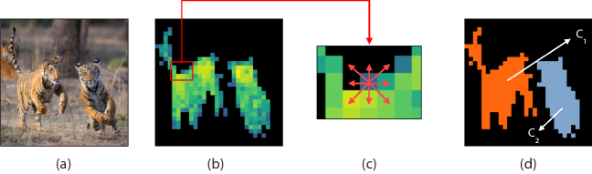
Figure 2: A schematic illustration of the spatial entropy. (a) The original image. (b) The thresholded similarity map $B^{h}$ (zero values shown in black). (c) The 8-connectivity relation used to group non-zero elements in $B^{h}$. (d) The resulting two connected components ($C_{1}$ and $C_{2}$).

In order to extract a set of connected components containing the largest values in $S^{h}$, we zero-out those elements of $S^{h}$ which are smaller than the mean value $m=1/n\sum_{(x,y)\in\{1,...,k\}^{2}}S^{h}_{x,y}$:

$$B_{x,y}^{h}=\mbox{ReLU}(S_{x,y}^{h}-m),\quad(x,y)\in\{1,...,k\}^{2},$$ (5)

where thresholding using $m$ corresponds to retain half of the total “mass” of Eq. 4. We can now use a standard algorithm (Grana ., 2010) to extract the connected components from $B^{h}$, obtained using an 8-connectivity relation between non-zero elements in $B^{h}$ (see Figure 2):

$$C^{h}=\{C_{1},...,C_{h_{r}}\}=\mbox{ConnectedComponents}(B^{h}).$$ (6)

$C_{j}$ ($1\leq j\leq h_{r}$) in $C^{h}$ is the set of coordinates ($C_{j}=\{(x_{1},y_{1}),...,(x_{n_{j}},y_{n_{j}})\}$) of the $j$-th connected component, whose cardinality ($n_{j}$) is variable, and such is the total number of components ($h_{r}$). Given $C^{h}$, we define the spatial entropy of $S^{h}$ ($\mathcal{H}(S^{h})$) as follows:

$$\mathcal{H}(S^{h})=-\sum_{j=1}^{h_{r}}P^{h}(C_{j})\log P^{h}(C_{j}),$$ (7)

$$P^{h}(C_{j})=\frac{1}{\lvert B^{h}\rvert}\sum_{(x,y)\in C_{j}}B_{x,y}^{h},$$ (8)

where $\lvert B^{h}\rvert=\sum_{(x,y)\in\{1,...,k\}^{2}}B_{x,y}^{h}$. Importantly, in Eq. 8, the probability of each region ($P^{h}(C_{j})$) is computed using all its elements, and this makes the difference with respect to a non-spatial entropy which is directly computed over all the individual elements in $S^{h}$, without considering the connectivity relation. Note that the less the number of components $h_{r}$ or the less uniformly distributed the probability values $P^{h}(C_{1}),...P^{h}(C_{h_{r}})$, the lower $\mathcal{H}(S^{h})$. Using Eq. 7, the spatial entropy loss is defined as:

$$\mathcal{L}_{se}=\frac{1}{H}\sum_{h=1}^{H}\mathcal{H}(S^{h}).$$ (9)

$\mathcal{L}_{se}$ is used jointly with the main task loss. For instance, in case of supervised training, we use: $\mathcal{L}_{tot}=\mathcal{L}_{ce}+\lambda\mathcal{L}_{se}$, where $\lambda$ is a weight used to balance the two losses.

4.2 Removing the skip connections

Raghu . (2021) empirically showed that, in the last blocks of ViT, the patch token representations are mostly propagated from the previous layers using the skip connections (Section 1). We presume this is (partially) due to the fact that only the [CLS] token is used as input to the classification MLP head (Section 3), thus, during training, the last-block patch token embeddings are usually neglected. Moreover, Raghu . (2021) show that the effective receptive field (Luo ., 2017) of each block, when computed after the MSA skip connections, is much smaller than the effective receptive field computed before the MSA skip connections. Both empirical observations lead to the conclusion that the MSA skip connections in the last blocks may be detrimental for the representation capacity of the final patch token embeddings. This problem is emphasized when using our spatial entropy loss, since it is computed using the attention maps of the last-block MSA (Section 4.1). For these reasons, we propose to remove the MSA skip connections in the last block ($L$). Specifically, in the $L$-th block, we replace Eq. 1-2 with:

$$\boldsymbol{z}^{\prime}=\mbox{MSA}(\mbox{LN}(\boldsymbol{z}^{L-1})),$$ (10)

$$\boldsymbol{z}^{L}=\mbox{MLP}(\boldsymbol{z}^{\prime})+\boldsymbol{z}^{\prime}.$$ (11)

Note that, in addition to removing the MSA skip connections (Eq. 10), we also remove the subsequent LN (Eq. 11), because we empirically observed that this further improves the VT accuracy (see Section 5.1).

4.3 Discussion

In this section, we discuss and motivate the choices made in Section 4.1 and Section 4.2. First, we use $S^{h}$, extracted before the softmax (Eq. 3) because, using the softmax, the network can “cheat”, by increasing the norm of the vectors $\boldsymbol{q}_{CLS}$ and $\boldsymbol{k}_{x,y}$ ($(x,y)\in\{1,...,k\}^{2}$). As a result, the dot product $<\boldsymbol{q}_{CLS},\boldsymbol{k}_{x,y}>$ also largely increases, and the softmax operation (based on the exponential function) enormously exaggerates the difference between the elements in $S^{h}$, generating a very peaked distribution, which zeros-out non-maxima $(x,y)$ elements. We observed that, when using the softmax, the VT is able to minimize Eq. 9 by producing single-peak similarity maps which have a 0 entropy, each being composed of only one connected component with only one single token (i.e., $h_{r}=1$ and $n_{j}=1$).

Second, the spatial entropy (Eq. 7) is computed for each head separately and then averaged (Eq. 9) to allow each head to focus on different image regions. Note that, although computing the connected components (Eq. 6) is a non-differentiable operation, $C^{h}$ is only used to “pool” the values of $B^{h}$ (Eq. 8), and each $C_{j}$ can be implemented as a binary mask (more details in the Appendix, where we also compare $\mathcal{L}_{se}$ with other solutions). It is also important to note that, although a smaller number of connected components ($h_{r}$) can decrease $\mathcal{L}_{se}$, this does not force the VT to always produce a single connected component (i.e., $h_{r}=1$) because of the contribution of the main task loss (e.g., $\mathcal{L}_{ce}$). For instance, Figure 1 (c) shows 4 big connected components which correctly correspond to the non-occluded parts of the bear and their reflections into the river, respectively.

Finally, we remove the MSA skip connections only in the last block (Eq. 10-11) because, according to the results reported in (Raghu ., 2021), removing the skip connections in the ViT intermediate blocks brings to an accuracy drop. In contrast, in Section 5.1 we show that our strategy, which keeps the ViT architecture unchanged apart from the last block, is beneficial even when used without our spatial entropy loss. Similarly, in preliminary experiments in which we used the spatial entropy loss also in other intermediate layers ($l<L$), we did not observe any significant improvement. In the rest of this paper, we refer to our full method SAR as composed of the spatial entropy loss (Section 4.1) and the last-block MSA skip connection and LN removal (Section 4.2).

5 Experiments

In Section 5.1 we analyse the contribution of the spatial entropy loss and the skip connection removal. In Section 5.2 we show that SAR improves ViT in different training-testing scenarios and with different downstream tasks. In Section 5.3 we analyse the properties of the attention maps generated using SAR. In the Appendix, we provide additional experiments and we use SAR jointly with fully self-supervised learning approaches. Each model was trained using 8 NVIDIA V100 32GB GPUs.

5.1 Ablation study

In this section, we analyse the influence of the $\lambda$ value (Section 4.1), the removal of the skip connections and the LN in the last ViT block (Section 4.2), and the use of the spatial entropy loss (Section 4.1). In all the ablation experiments, we use ImageNet-100 (IN-100) (Tian ., 2020; T. Wang  Isola, 2020), which is a subset of 100 classes of ImageNet, and ViT-S/16, a 22 million parameter ViT (Dosovitskiy ., 2021) trained with $224\times 224$ resolution images and $14\times 14$ patches tokens ($k=14$) with a patch resolution of $16\times 16$ (Touvron ., 2020). Moreover, in all the experiments in this section, we adopt the training protocol and the data-augmentations described in (Z. Liu ., 2021). Note that these data-augmentations include, among other things, the use of Mixup (Zhang ., 2018) and CutMix (Yun ., 2019) (which are also used in all the supervised classification experiments of Section 5.2), and this shows that our entropy loss can be used jointly with “image-mixing” techniques.

In Table 4 (a), we train from scratch all the models using 100 epochs and we show the impact on the test set accuracy using different values of $\lambda$. In the experiments of this table, we use our loss function ($\mathcal{L}_{tot}=\mathcal{L}_{ce}+\lambda\mathcal{L}_{se}$) and we remove both the skip connections and the LN in the last block (Eq. 10-11), thus the column $\lambda=0$ corresponds to the result reported in Table 4 (b), Row “C” (see below). In the rest of the paper, we use the results obtained with this setting (IN-100, 100 epochs, etc.) and the best $\lambda$ value ($\lambda=0.01$) for all the other datasets, training scenarios (e.g., training from scratch, fine-tuning, fully self-supervised learning) and VT architectures (e.g., ViT, CvT, PVT, etc.). In fact, although a higher accuracy can very likely be obtained by tuning $\lambda$, our goal is to show that SAR is an easy-to-use regularization approach, even without tuning its only hyperparameter.

Table 1: IN-100. (a) Influence of the spatial entropy loss weight $\lambda$ (100 training epochs). (b) Analysis of the different components of SAR (100 epochs). (c) Influence of the number of epochs.

$\lambda$	Top-1 Acc.
0	75.72
0.001	75.82
0.005	76.16
0.01	76.72
0.05	76.22
0.1	75.88

Table 2: (a)

Model	Top-1 Acc.
A: Baseline	74.22
B: A + no MSA skip connections	74.64 (+0.42)
C: B + no LN	75.72 (+1.5)
D: C + no MLP skip connections	73.76 (-0.46)
E: A + spatial entropy loss	74.78 (+0.56)
F: A + SAR	76.72 (+2.5)

Table 3: (b)

Model	Top-1 Acc.
	100 ep.	300 ep.
ViT-S/16	74.22	80.82
ViT-S/16+SAR	76.72 (+2.5)	85.24 (+4.42)

Table 4: (c)

In Table 4 (b), we train from scratch all the models using 100 epochs and Row “A” corresponds to our run of the original ViT-S/16 (Eq. 1-2). When we remove the MSA skip connections (Row “B”), we observe a $+0.42$ points improvement, which becomes $+1.5$ if we also remove the LN (Row “C”). This experiment confirms that the last block patch tokens can learn more useful representations if we inhibit the MSA identity path (Eq. 10-11). However, if we also remove the skip connections in the subsequent MLP layer (Row “D”), the results are inferior to the baseline. Finally, when we use the spatial entropy loss with the original architecture (Row “E”), the improvement is marginal, but using $\mathcal{L}_{se}$ jointly with Eq. 10-11 (full model, Row “F”), the accuracy boost with respect to the baseline is much stronger. Table 4 (c) compares training with 100 and 300 epochs and shows that, in the latter case, SAR can reach a much higher relative improvement with respect to the baseline ($+4.42$).

5.2 Main results

Sample efficiency. In order to show that SAR can alleviate the need of large labeled datasets (Section 1), we follow a recent trend of works (Y. Liu ., 2021; El-Nouby ., 2021; Cao  Wu, 2021) where VTs are trained from scratch on small-medium datasets (without pre-training on ImageNet). Specifically, we strictly follow the training protocol proposed by El-Nouby . (2021), where 5,000 epochs are used to train ViT-S/16 directly on each target dataset. The results are shown in Table 2, which also provides the number of training and testing samples of each dataset, jointly with the accuracy values of the baseline (ViT-S/16, trained in a standard way, without SAR), both reported from El-Nouby . (2021). Table 2 shows that SAR can drastically improve the ViT-S/16 accuracy on these small-medium datasets, with an improvement ranging from $+18.17$ to $+30.78$ points. These results, jointly with the results obtained on IN-100 (Table 4 (c)), show that SAR is particularly effective in boosting the performance of ViT when labeled training data are scarce.

We further analyze the impact of the amount of training data using different subsets of IN-100 with different sampling ratios (ranging from $25\%$ to $75\%$, with images randomly selected). We use the same training protocol of Table 4 (c) (e.g., 100 training epochs, etc.) and we test on the whole IN-100 validation set. Table 3 shows the results, confirming that, with less data, the accuracy boost obtained using SAR can significantly increase (e.g., with $75\%$ of the data we have a 10.5 points improvement).

Table 2: Training from scratch on small-medium datasets. The baseline (ViT-S/16) results are reported from (El-Nouby ., 2021).

Dataset	$\#$ Train samples	$\#$ Test samples	$\#$ Classes	ViT-S/16	ViT-S/16+SAR
Stanford Cars	8,144	8,041	196	35.3	64.65 (+29.35)
Clipart	34,019	14,818	345	41.0	64.95 (+23.95)
Painting	52,867	22,892	345	38.4	57.11 (+18.17)
Sketch	49,115	21,271	345	37.2	62.98 (+30.78)

Table 3: IN-100 experiments with different sampling ratios (100 epochs).

Model	Top-1 Acc.
	0.25	0.50	0.75	1.00
ViT-S/16	21.66	29.86	35.62	74.22
ViT-S/16+SAR	29.06 (+7.4)	38.02 (+8.16)	46.12 (+10.5)	76.72 (+2.5)

Training on ImageNet-1K. We extend the previous results training ViT on ImageNet-1K (IN-1K), and comparing SAR with the baseline (ViT-S/16, trained in a standard way, without SAR), and with the Dense Relative Localization (DRLoc) loss (Y. Liu ., 2021), which, similarly to SAR, is based on an auxiliary self-supervised task used to regularize VTs training (Section 2). DRLoc encourages the VT to learn spatial relations within an image by predicting the relative distance between the $(x,y)$ positions of randomly sampled output embeddings from the $k\times k$ grid of the last layer $L$. Table 4 shows that SAR can boost the accuracy of ViT of almost 1 point without any additional learnable parameters or drastic architectural changes, and this gain is higher than DRLoc. The reason why the relative improvement is smaller with respect to what was obtained with smaller datasets is likely due to the fact that, usually, regularization techniques are mostly effective with small(er) datasets (Y. Liu ., 2021; Balestriero ., 2022). Nevertheless, Fig. 3 shows that SAR can be used jointly with large datasets to significantly speed-up training. For instance, ViT-S/16 + SAR, with 100 epochs, achieves almost the same accuracy as the baseline trained with 150 epochs, while we surpass the final baseline accuracy ($79.8\%$ at epoch 300) with only 250 training epochs ($79.9\%$ at epoch 250). Finally, the two regularization approaches (SAR and DRLoc) can potentially be combined, but we leave this for future work.

Table 4: IN-1K experiments (300 training epochs). ^† This result has been obtained by us using the publicly available code taken from (Y. Liu ., 2021).

Method	Top-1 Acc.
ViT-S/16 (Touvron ., 2020)	79.8
ViT-S/16 + DRLoc†	80.2 (+0.4)
ViT-S/16 + SAR	80.7 (+0.9)

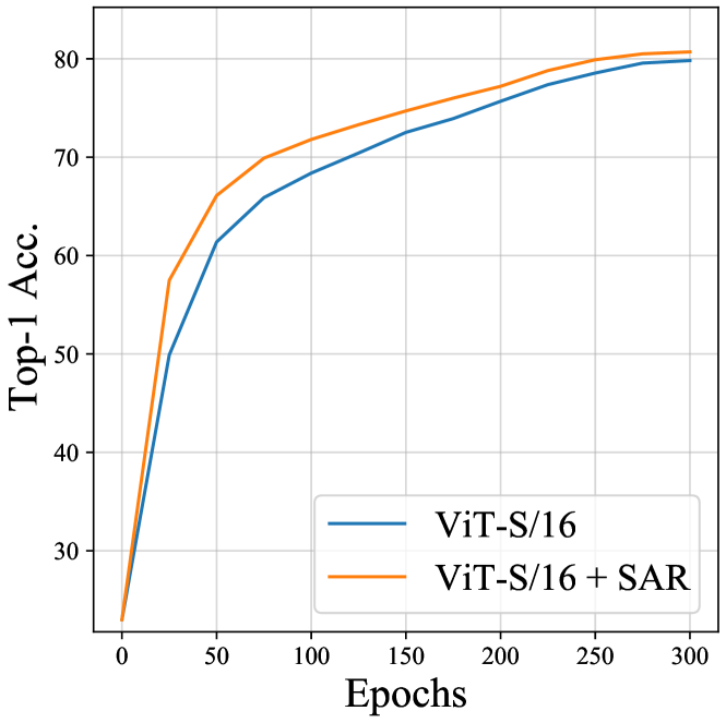
Figure 3: IN-1K, validation set accuracy with respect to the number of training epochs.

Transfer learning with object detection and image segmentation tasks. We further analyze the quality of the models pre-trained on IN-1K using object detection and semantic segmentation downstream tasks. Specifically, we use ViTDet (Y. Li ., 2022), a recently proposed object detection/segmentation framework in which a (standard) pre-trained ViT backbone is adapted only at fine-tuning time in order to generate a feature pyramid to be used for multi-scale object detection or image segmentation. Note that, as mentioned in Section 1, hybrid approaches which are based on ad hoc architectures are not suitable from this framework, because they need to redesign their backbone and introduce a feature pyramid also in the pre-training stage (Y. Li ., 2022; W. Wang ., 2021). Conversely, we use the pre-trained networks whose results are reported in Table 4, where the baseline is ViT-S/16 and our approach corresponds to ViT-S/16 + SAR. For the object detection task, following (Girshick, 2015), we use the trainval set of PASCAL VOC 2007 and 2012 (Everingham ., 2010) (16.5K training images) to fine-tune the two models using ViTDet, and the test set of PASCAL VOC 2007 for evaluation. The results, reported in Table 5, show that the model pre-trained using SAR outperforms the baseline of more than 2 points, which is an increment even larger that the boost obtained in the classification task used during pre-training (Table 4). Similarly, for the segmentation task, we use PASCAL VOC-12 trainval for fine-tuning and PASCAL VOC-12 test for evaluation. Table 6 shows that the model pre-trained with SAR achieves an improvement of more than 2.5 mIoU points compared to the baseline. These detection and segmentation improvements confirm that the local inductive bias introduced in ViT using SAR can be very useful for localization tasks, especially when the fine-tuning data are scarce like in PASCAL VOC.

Table 5: Object detection on PASCAL VOC 2007, evaluated using mean Average Precision (mAP).

Model	mAP
ViT-S/16	77.1
ViT-S/16 + SAR	79.2 (+2.1)

Table 6: Semantic segmentation on PASCAL VOC 2012, evaluated using mean Intersection over Union (mIoU).

Model	mIoU
ViT-S/16	66.17
ViT-S/16 + SAR	68.68 (+2.51)

Transfer learning with different fine-tuning protocols. In this battery of experiments, we evaluate SAR in a transfer learning scenario with classification tasks. We adopt the four datasets used in (Dosovitskiy ., 2021; Touvron ., 2020; X. Chen ., 2021; Caron ., 2021): CIFAR-10 and CIFAR-100 (Krizhevsky ., 2009), Oxford Flowers102 (Nilsback  Zisserman, 2008), and Oxford-IIIT-Pets (Parkhi ., 2012). The standard transfer learning protocol consists in pre-training on IN-1K, and then fine-tuning on each dataset. This corresponds to the first row in Table 7, where the IN-1K pre-trained model is ViT-S/16 in Table 4. The next three rows show different pre-training/fine-tuning configurations, in which we use SAR in one of the two phases or in both (see the Appendix for more details). All the configurations lead to an overall improvement of the accuracy with respect to the baseline, and show that SAR can be used flexibly. For instance, SAR can be used when fine-tuning a VT trained in a standard way, without the need to re-train it on ImageNet.

Table 7: Transfer learning results (100 epochs fine-tuning). The first row corresponds to a standard fine-tuning protocol, while the other configurations include SAR either in the pre-training or in the fine-tuning stage.

SAR	SAR	CIFAR-10	CIFAR-100	Flowers	Pets
pre-training	fine-tuning
✗	✗	98.59	88.95	95.07	92.21
✓	✗	98.69 (+0.1)	89.19 (+0.24)	96.05 (+0.98)	92.7 (+0.49)
✗	✓	98.72 (+0.13)	88.95	95.1 (+0.03)	92.34 (+0.13)
✓	✓	98.65 (+0.06)	89.21 (+0.26)	96.1 (+1.03)	92.7 (+0.49)

Out-of-distribution testing. We test the robustness of our ViT trained with SAR when the testing distribution is different from the training distribution. Specifically, following Bai . (2021), we use two different testing sets: (1) ImageNet-A (Hendrycks ., 2019), which are real-world images but collected from challenging scenarios (e.g., occlusions, fog scenes, etc.), and (2) ImageNet-C (Hendrycks  Dietterich, 2018), which is designed to measure the model robustness against common image corruptions. Note that training is done only on IN-1K. Thus, in Table 8, ViT-S/16 and ViT-S/16 + SAR correspond to the models we trained on IN-1K whose results on the IN-1K standard validation set are reported in Table 4. ImageNet-A and ImageNet-C are used only for testing, hence they are useful to assess the behaviour of a model when evaluated on a distribution different from the training distribution (Bai ., 2021). The results reported in Table 8 show that SAR can significantly improve the robustness of ViT (note that, with the mCE metric, the lower the better (Bai ., 2021)). We presume that this is a side-effect of our spatial entropy loss minimization, which leads to heads usually focusing on the foreground objects and, therefore, reducing the dependence with respect to the background appearance variability distribution.

Table 8: Out-of-distribution testing on ImageNet-A (IN-A) and ImageNet-C (IN-C).

Model	IN-A (Acc. $\uparrow$)	IN-C (mCE $\downarrow$)
ViT-S/16	19.2	52.8
ViT-S/16 + SAR	22.39 (+3.19)	51.6 (-1.2)

Different VT architectures. Finally, we show that SAR can be used with VTs of different capacities and with architectures different from ViT. For this purpose, we plug SAR into the following VT architectures: ViT-S/16 (Touvron ., 2020), T2T (L. Yuan ., 2021), PVT (W. Wang ., 2021) and CvT (Wu ., 2021). Specifically, T2T, PVT and CvT are hybrid architectures, which use typical CNN mechanisms to introduce a local inductive bias into the VT training (Sections 1 and 2). We omit other common frameworks such as, for instance, Swin (Z. Liu ., 2021) because of the lack of a [CLS] token in their architecture. Although the [CLS] token used, e.g, in Section 4.1 to compute $S^{h}$, can potentially be replaced by a vector obtained by average-pooling all the patch embeddings, we leave this for future investigations. Moreover, for computational reasons, we focus on small-medium capacity VTs (see Table 10 for details on the number of parameters of each VT). Importantly, for each tested method, we use the original training protocol developed by the corresponding authors, including, e.g., the learning rate schedule, the batch size, the VT-specific hyperparameter values and the data-augmentation type used to obtain the corresponding published results, both when we train the baseline and when we train using SAR. Moreover, as usual (Section 5.1), we keep fixed the only SAR hyperparameter ($\lambda=0.01$). Although better results can likely be obtained by adopting the common practice of hyperparameter tuning (including the VT-specific hyperparameters), our goal is to show that SAR can be easily used in different VTs, increasing their final testing accuracy. The results reported in Table 9 and Table 10 show that SAR improves all the tested VTs, independently of their specific architecture, model capacity or training protocol. Note that both PVT and CvT have a final grid resolution of $7\times 7$, which is smaller than the $14\times 14$ grid used in ViT and T2T, and this probably has a negative impact on our spatial based entropy loss.

Overall, the results reported in Table 9 and Table 10: (1) Confirm that SAR is mostly useful with smaller datasets (being the relative improvements on IN-100 significantly larger than those obtained on IN-1K). (2) Show that the object-based inductive bias introduced when training with SAR is (partially) complementary with respect to the local bias embedded in the hybrid VT architectures, as witnessed by the positive boost obtained when these VTs are used jointly with SAR. (3) Show that, on IN-1K, the accuracy of ViT-S/16 + SAR is comparable with the hybrid VTs (without SAR). However, the advantage of ViT-S/16 + SAR is its simplicity, which does not need drastic architectural changes to the original ViT architecture, where the latter is quickly becoming a de facto standard in many vision and vision-language tasks (Section 2).

Table 9: IN-100 experiments with different VTs (100 training epochs). The results of the baselines have been obtained by us using the corresponding publicly available code.

Model	Top-1 Acc.
ViT-S/16	74.22
ViT-S/16 + SAR	76.72 (+2.5)
T2T-ViT-14	82.42
T2T-ViT-14 + SAR	83.96 (+1.54)
PVT-Small	76.57
PVT-Small + SAR	77.78 (+1.21)
CvT-13	83.38
CvT-13 + SAR	85.20 (+1.82)

Table 10: IN-1K experiments with different VTs (300 training epochs). All results but ours are reported from the corresponding paper. The number of parameters are in millions.

Module	Param.	Acc.
ViT-S/16	22	79.8
ViT-S/16 + SAR	22	80.7 (+0.9)
T2T-ViT-14	21.5	81.5
T2T-ViT-14 + SAR	21.5	81.9 (+0.4)
PVT-Small	24.5	79.8
PVT-Small + SAR	24.5	79.84 (+0.04)
CvT-13	20	81.6
CvT-13 + SAR	20	81.8 (+0.2)

ViT-S/16

ViT-S/16+SAR

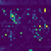
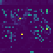
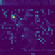
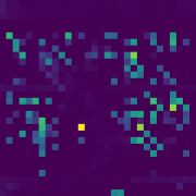
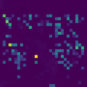
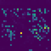
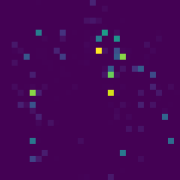
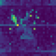
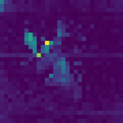
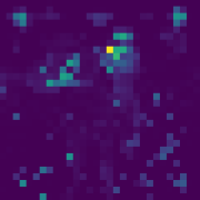
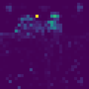
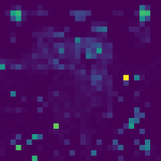
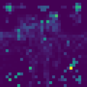
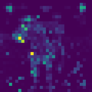
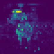
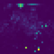
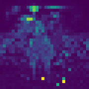
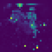
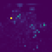
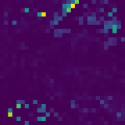
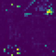
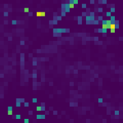
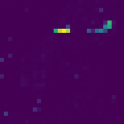
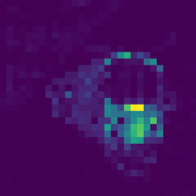
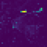
Figure 4: A qualitative comparison between the attention maps generated by ViT-S/16 (left) and ViT-S/16 + SAR (right). For each image, we show all the 6 attention maps ($A^{h}$) corresponding to the 6 last-block heads, computed using only the [CLS] token query.

5.3 Attention map analysis

This section qualitatively and quantitatively analyses the attention maps obtained using SAR. Note that, as mentioned in Sections 1 and 2, we do not directly use the attention map clusters for segmentation tasks or as input to a post-processing step. Thus, the goal of this analysis is to show that the spatial entropy loss minimization effectively results in attention maps with spatial clusters, leaving their potential use for a segmentation-based post-processing as a future work.

Figure 4 visually compares the attention maps obtained with ViT-S/16 and ViT-S/16 + SAR. As expected, standard training generates attention maps with a widely spread structure. Conversely, using SAR, a semantic segmentation structure clearly emerges. In the Appendix, we show additional results. For a quantitative analysis, we follow the protocol used in (Caron ., 2021; Naseer ., 2021), where the Jaccard similarity is used to compare the ground-truth segmentation masks of the objects in PASCAL VOC-12 with the thresholded attention masks of the last ViT block. Specifically, the attention maps of all the heads are thresholded to keep $60\%$ of the mass, and the head with the highest Jaccard similarity with the ground-truth is selected (Caron ., 2021; Naseer ., 2021). Table 11 shows that SAR significantly improves the segmentation results, quantitatively confirming the qualitative analysis in Figure 4.

Table 11: A comparison of the segmentation properties of the attention maps on PASCAL VOC-12.

Model	Jaccard similarity ($\uparrow$)
ViT-S/16	19.18
ViT-S/16 + SAR	31.19 (+12.01)

6 Conclusions

In this paper we proposed SAR, a regularization method which exploits the connectedness property of the objects to introduce a local inductive bias into the VT training. By penalizing spatially disordered attention maps, an additional self-supervised signal can be extracted from the sample images, thereby reducing the reliance on large numbers of labeled training samples. Using different downstream tasks and training-testing protocols (including fine-tuning and out-of-distribution testing), we showed tha SAR can significantly boost the accuracy of a ViT backbone, especially when the training data are scarce. Despite SAR can also be used jointly with hybrid VTs, its main advantage over the latter is the possibility to be easily plugged into the original ViT backbone, whose architecture is widely adopted in many vision and vision language tasks.

Limitations. Since training VTs is very computationally expensive, in our experiments we used only small/medium capacity VTs. We leave the extension of our empirical analysis to larger capacity VTs for the future. For the same computational reasons, we have not tuned hyperparameters on the datasets. However, we believe that the SAR accuracy improvement, obtained in all the tested scenarios without hyperparameter tuning, further shows its robustness and ease to use.

Appendix A Pseudo-code of the Spatial Entropy loss

Figure 5 shows the pseudo-code for computing $\mathcal{L}_{se}$ (Eq. 9). The goal is twofold: to show how easy is to compute $\mathcal{L}_{se}$, and how to make it differentiable. Specifically, Eq. 6 is based on a connected component algorithm which is not differentiable. However, once $C^{h}$ is computed, each element $C_{j}\in C^{h}$ ($C_{j}=\{(x_{1},y_{1}),...,(x_{n_{j}},y_{n_{j}})\}$) can be represented as a binary mask $M_{j}$, defined as:

$$M_{j}[x,y]=\begin{cases}1,&\text{if }(x,y)\in C_{j}\\ 0&\text{otherwise}\end{cases}$$ (12)

Using Eq. 12, we compute the probability $P^{h}(C_{j})$ of the component $C_{j}$ using matrix multiplication, which is done efficiently on GPUs. In practice, Eq. 8 is computed as:

$$P^{h}(C_{j})=\frac{1}{|B^{h}|}\sum_{(x,y)}B_{x,y}^{h}\odot M_{j}[x,y],$$ (13)

where $\odot$ is the element-wise product. This implementation makes it is possible to back-propagate the spatial entropy loss even if the connected component algorithm is not differentiable.

⬇

# bs : batch size

# H : number of heads

# k x k : size of the embedding grid

# S : defined in Eq. 4 (main paper),

# tensor with shape [bs, H, k, k]

\pardef SpatialEntropy(S, eps=1e-9):

bs, H, k, _ = S.size()

m = torch.mean(S, dim=[2, 3], keepdim=True)

B = torch.relu(S - m) + eps

\parwith torch.no_grad():

batch_idxs, head_idxs, M = connected_components(B)

\parp_u = torch.sum(B[batch_idxs, head_idxs] * M, dim=[2, 3])

p_n = p_u / torch.sum(B, dim=[2, 3])

SE = -torch.sum((p_n * torch.log(p_n)) / (bs * H)

return SE

\par

Figure 5: PyTorch-like pseudocode of the Spatial Entropy loss.

Appendix B Comparing the spatial entropy loss with other solutions

In our preliminary experiments, we replaced the spatial entropy loss with a different loss based on a total variation denoising (Rudin ., 1992) criterion, which we formulated as:

$$\mathcal{L}_{tv}=\frac{1}{H}\sum_{h=1}^{H}\sum_{(x,y)\in\{1,...,k\}^{2}}|S_{x,y}^{h}-S_{x,y+1}^{h}|+\\ |S_{x,y}^{h}-S_{x+1,y}^{h}|.$$ (14)

However, $\mathcal{L}_{tv}$ drastically underperforms $\mathcal{L}_{se}$ and tends to produce blurred (more uniform) attention maps. The main difference between $\mathcal{L}_{tv}$ and $\mathcal{L}_{se}$ is that the thresholding (Eq. 5) and the adjacency-based clustering (Eq. 6) operations in $\mathcal{L}_{se}$ group together image regions of variable size and shape which have in common high attention scores for a specific head, and, therefore, they presumably represent the same semantics (e.g., a specific object). In contrast, $\mathcal{L}_{tv}$ compares patch tokens which are adjacent to each other (e.g., $S_{x,y}^{h}$ and $S_{x,y+1}^{h}$) but which do not necessarily share the same semantics (e.g., $S_{x,y}^{h}$ may belong to the background while $S_{x,y+1}^{h}$ belongs to a foreground object). Thus, the implicit local inductive bias of the two losses is different: in case of $\mathcal{L}_{se}$, the inductive bias is that the image regions corresponding to the highest attention scores (for a specific head) should be spatially grouped in few, big “blobs”, while, in the case of $\mathcal{L}_{tv}$, the inductive bias is that generic adjacent regions should have similar attention scores.

Finally, we have empirically tested slightly different similarity metrics. For instance, replacing Eq. 4 with a cosine similarity computed as:

$$\hat{S}_{x,y}^{h}=\frac{<\boldsymbol{q}_{CLS}^{h},\boldsymbol{k}_{x,y}^{h}>}{||\boldsymbol{q}_{CLS}^{h}||||\boldsymbol{k}_{x,y}^{h}||},\quad(x,y)\in\{1,...,k\}^{2},$$ (15)

and keeping all the rest unchanged (e.g., Eq. 5-Eq. 9), we get a slightly lower accuracy when training on IN-100 (76.25 top-1 accuracy versus 76.72 in Table 4 (c)). This is likely due to the fact that $\hat{S}^{h}$ in Eq. 15 does not correspond to the metric used to compute the attention for the main task loss (Eq. 3). Thus, merging the main task loss (e.g., the cross entropy loss) with the spatial entropy loss may be more difficult.

Appendix C Self-supervised experiments

In this section, we use SAR in a fully self-supervised scenario. Analogously to all the other experiments of this paper, we keep fixed $\lambda=0.01$ and we use the hyperparameters of each tested VT-based method without any hyperparameter tuning. Since self-supervised learning algorithms are very time consuming, we use IN-100, which is a medium-size dataset. We plug SAR on top of two state-of-the-art VT-based self-supervised learning algorithms: MoCo-v3 (X. Chen ., 2021) and DINO (Caron ., 2021) (Section 2). When we use MoCo-v3, in $\mathcal{L}_{tot}$ (Section 4.1), we replace the cross-entropy loss ($\mathcal{L}_{ce}$) with the contrastive loss used in (X. Chen ., 2021). Similarly, when we use DINO, we use as the main task loss the “self-distillation” proposed in (Caron ., 2021), jointly with its multi-crop strategy. We use the official code of MoCo-v3 and DINO and we strictly follow the algorithms and the training protocols of the baseline methods, including all the default hyperparameters suggested by the corresponding authors. However, for computational reasons, we used a 1024 batch size for MoCo-v3 and MoCo-v3 + SAR, and a batch size of 512 for DINO and DINO + SAR. The VT backbone is ViT-S/16 for all the methods. More details in Appendix E.

We evaluate all models (with and without SAR) using the standard self-supervised evaluation protocol, consisting in freezing the network after training and then training a linear classifier on top of the frozen features (Caron ., 2021; X. Chen ., 2021). The results are reported in Table 14 (a), and show that, on IN-100, SAR significantly improves these state-of-the-art algorithms, including DINO (which inspired our work).

We qualitatively compare the attention maps obtained with and without SAR in Figure 6 (MoCo-v3) and Figure 7 (DINO). Figure 6 shows that, in MoCo-v3 + SAR, the head-specific attention maps focus on slightly different aspects of the main object, while in MoCo-v3, the attention is much more “disordered” (spread over the whole image). On the other hand, when comparing DINO with DINO + SAR (Figure 7), the attention map differences are more subtle. However, the higher inter-head variability in DINO + SAR is one interesting difference. For instance, while DINO’s maps usually focus only on the main foreground object, in DINO + SAR, different heads cover different foreground objects (e.g., the cat and the sink in Row 11) or different background regions (e.g., the road and the sky in the “train” figure of Row 5). This difference is probably due to the difference in how DINO and DINO + SAR are optimized. In fact, in DINO, the only source of supervision is the comparison between two different views of the same image (Section 2), which likely encourages the network to focus on the objects most frequently in common. On the other hand, in DINO + SAR, the creation of connected regions with large attention values into each head’s map is also encouraged using $\mathcal{L}_{se}$.

These qualitative observations are confirmed by the quantitative analysis reported in Table 14 (b), where we follow the protocol described in Section 5.3. SAR increases the Jaccard similarity of both self-supervised algorithms.

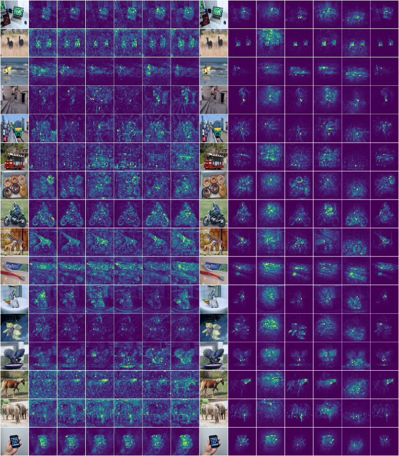
MoCo-v3	MoCo-v3 + SAR

Figure 6: A qualitative comparison between the attention maps generated by MoCo-v3 and MoCo-v3 + SAR with the ViT-S/16 backbone (training on IN-100). For each image, we show all the 6 attention maps ($A^{h}$) corresponding to the 6 last-block heads, computed using only the [CLS] token query.

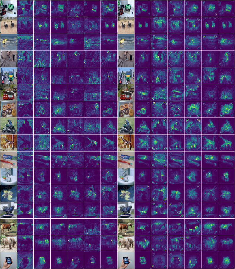
DINO	DINO + SAR

Figure 7: A qualitative comparison between the attention maps generated by DINO and DINO + SAR with the ViT-S/16 backbone (training on IN-100).

Table 12: Self-supervised training on IN-100 (300 epochs). (a) Accuracy on IN-100 evaluated through linear probing and a single testing crop. (b) Segmentation properties of the corresponding attention maps evaluated on PASCAL VOC-12. The results of the baselines have been obtained by us using the corresponding publicly available code.

Method	Top-1 Acc.
MoCo-v3	77.60
MoCo-v3 + SAR	78.88 (+1.28)
DINO	77.42
DINO + SAR	79.90 (+2.48)

Table 13: (a)

Method	Jaccard similarity
MoCo-v3	27.40
MoCo-v3 + SAR	33.10 (+6.17)
DINO	35.06
DINO + SAR	35.28 (+0.22)

Table 14: (b)

Appendix D An additional qualitative analysis of the attention maps

In this section, we extend the analysis of Section 5.3 providing additional visualizations of the attention maps obtained using supervised training on IN-1K.

Figure 8 shows the attention maps of ViT-S/16 and ViT-S/16 + SAR. These attention maps show that the ViT-S/16 attention scores are spread over all the image, while in ViT-S/16 + SAR they are much more spatially clustered and usually focused on the main object(s) of the input image. For example, the first row shows that the heads of ViT-S/16 focus on the upper part of the image, and only the keyboard of the laptop emerges. Vice versa, from the ViT-S/16 + SAR attention heads, it is possible to recognise the shape and size of the laptop precisely. Similarly, the second last row shows an example where the input image contains some elephants. While the different heads of ViT-S/16 seem to focus mainly on the background, the first head of ViT-S/16 + SAR is clearly focused on the elephants. Importantly, these visualizations show that different heads of ViT-S/16 + SAR usually focus on different semantic concepts, which shows that there are no collapse phenomena using the spatial entropy loss (see Eq. 7 and the corresponding discussion in Section 4.3).

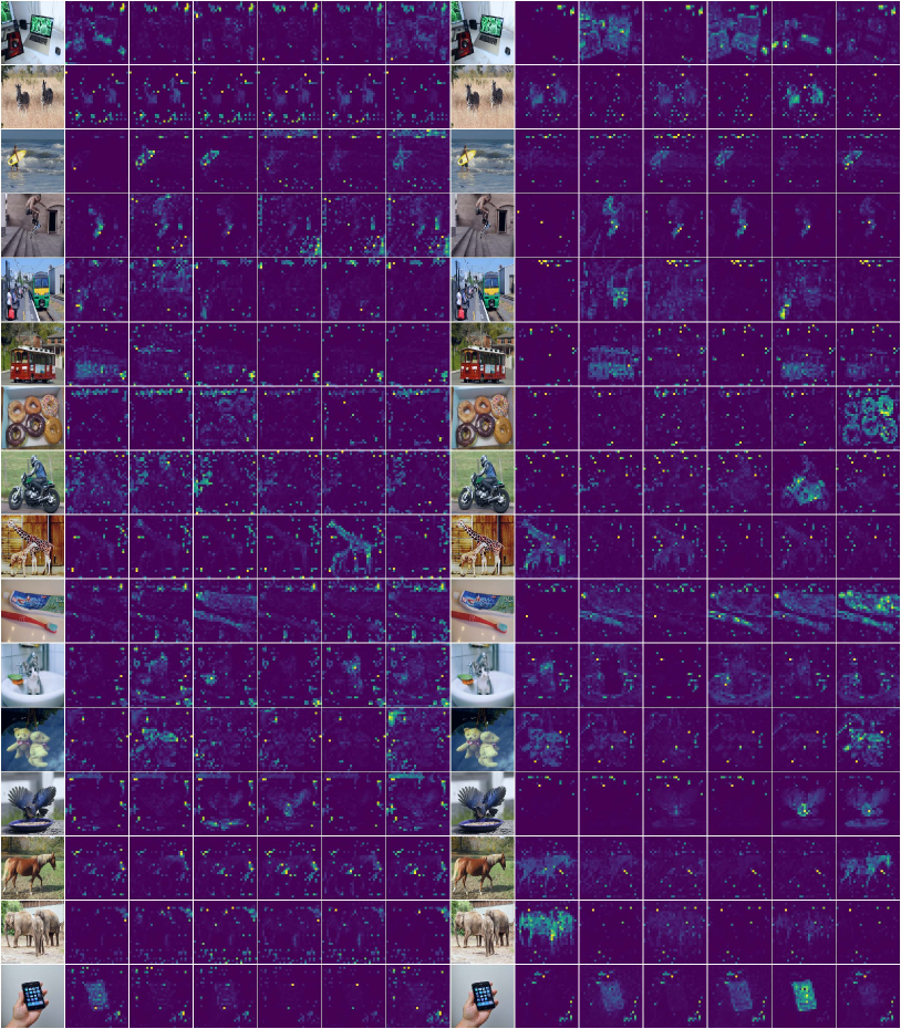
ViT-S/16	ViT-S/16 + SAR

Figure 8: A qualitative comparison between the attention maps generated by ViT-S/16 and ViT-S/16 + SAR (supervised case, training on IN-1K).

Appendix E Implementation details

In the following, we list the implementation details. Each model was trained using 8 NVIDIA V100 32GB GPUs. For computational reasons, the experiments of this paper have been done only once (and without hyperparameter tuning), thus we cannot report standard deviation values computed over multiple runs. However, this is the standard practice adopted by all the evaluation protocols used in this paper and by all the methods we have compared with.

E.1 ViT based models

We train our models using the public code of Touvron . (2020) for ViT and we modify the original code when we use SAR, as described in Section 4.2. The models are trained with a batch size of 1024, using the AdamW optimizer (Loshchilov  Hutter, 2019) with initial learning rate of 0.001, a cosine learning rate schedule, a weight decay of 0.05 and using the original data-augmentation protocol, including the use of Mixup (Zhang ., 2018) and CutMix (Yun ., 2019) for the supervised classification tasks.

E.2 Hybrid architectures

In all the supervised experiments, we used the officially released code for PVT (W. Wang ., 2021), T2T (L. Yuan ., 2021) and CvT (Wu ., 2021), strictly following the original training protocol for each architecture.

PVT and T2T are trained with batch size of 1024, using the AdamW optimizer with an initial learning rate of 0.001, momentum 0.9 and weight decay of 0.05. CvT is trained with a batch size of 2048 and an initial learning rate of 0.02, decayed with a cosine schedule. The data augumentations of the original articles are based on the DeiT protocol (Touvron ., 2020). We refer the reader to the original papers for further details. When we use SAR, we plug it on top of the original public code, following Section 4.2.

E.3 Object detection and semantic segmentation downstream tasks

Starting from the pretrained ViT-S/16 and ViT-S/16 + SAR models of Table 4, we follow (Y. Li . (2022)) to obtain a feature pyramid and a Mask-RCNN detector (He ., 2017). In both the object detection and the segmentation task, the models are fine-tuned for 25 epochs with the AdamW optimizer, learning rate of 0.0001 and linear warmup for the first 250 iterations. The input image is 512$\times$512 during training, augmented with random cropping and flipping. We used a batch size of 8 distributed on 4 GPUs.

E.4 Transfer learning with different fine-tuning protocols

We fine-tune the ViT-S/16 models pretrained on IN-1K (see Table 4), always keeping unchanged the VT architecture used in the pre-training stage. This is done to avoid making the adaptation task more difficult, since each of the four datasets used in Table 7 is composed of a relatively small number of samples. For instance, when SAR is used during pre-training but removed during fine-tuning (second row of Table 7), in the fine-tuning stage we use only $\mathcal{L}_{ce}$ for training but we do not re-introduce skip connections or LN layers in the last block (i.e., we use Eq. 10-Eq. 11 when fine-tuning). Conversely, when pre-training is done without SAR, which is introduced only in the fine-tuning stage (third row of Table 7), when fine-tuning, we use $\mathcal{L}_{tot}=\mathcal{L}_{ce}+\lambda\mathcal{L}_{se}$, but keeping the standard skip connections and the LN layer in the last block (Eq. 1-Eq. 2).

The models are fine-tuned for 100 epochs with a batch size of 512, and an initial learning rate of 0.0005 decayed with a cosine schedule.

E.5 Self-supervised experiments

In our self-supervised experiments, we adopt the original code for MoCo-v3 (X. Chen ., 2021) and DINO (Caron ., 2021) with a ViT-S/16 backbone. For computational reasons, we restrict our experiments training the models on IN-100 for 300 epochs. Moreover, to fit the available computational resources, we reduce the batch size to 1024 for MoCo-v3, while DINO is trained with the default multi-crop strategy $(2\times 224^{2}+10\times 96^{2})$, but with a batch size of 512. We thoroughly follow the authors’ specifications for the other hyperparameters. The results in Table 14 are obtained using a standard linear evaluation protocol in which the pretrained backbone is frozen, and a linear classifier is trained on top of it, using SGD for 100 epochs on IN-100.

Appendix F Dataset licensing details

CIFAR-10, CIFAR-100 are released to the public with a non-commercial research and/or educational use. Oxford flower102 is released to the public with an unknown license through its website, and we assume a non-commercial research and/or educational use. ImageNet annotations have a non-commercial research and educational license. PASCAL VOC 2012 images abide by the Flickr Terms of Use. Stanford Cars images have a non-commercial research and educational license ClipArt, Painting and Sketches are part of the DomainNet dataset which is released under a fair use license. The ImageNet-A and ImageNet-C images are released with unknown licence, so we refer to the original authors to use these datasets.

References

- \bibcommenthead
- Alayrac \BOthers. (\APACyear2022) \APACinsertmetastarDBLP:journals/corr/abs-2204-14198{APACrefauthors}Alayrac, J., Donahue, J., Luc, P., Miech, A., Barr, I., Hasson, Y.\BDBLSimonyan, K. \APACrefYearMonthDay2022. \BBOQ\APACrefatitleFlamingo: a Visual Language Model for Few-Shot Learning Flamingo: a visual language model for few-shot learning.\BBCQ \APACjournalVolNumPagesarXiv:2204.14198. \PrintBackRefs\CurrentBib
- Altieri \BOthers. (\APACyear2018) \APACinsertmetastaraltieri2018spatentropy{APACrefauthors}Altieri, L., Cocchi, D.\BCBL Roli, G. \APACrefYearMonthDay2018. \BBOQ\APACrefatitleSpatEntropy: Spatial Entropy Measures in R SpatEntropy: Spatial Entropy Measures in R.\BBCQ \APACjournalVolNumPagesarXiv:1804.05521. \PrintBackRefs\CurrentBib
- Asano \BOthers. (\APACyear2020) \APACinsertmetastarDBLP:conf/iclr/AsanoRV20a{APACrefauthors}Asano, Y.M., Rupprecht, C.\BCBL Vedaldi, A. \APACrefYearMonthDay2020. \BBOQ\APACrefatitleSelf-labelling via simultaneous clustering and representation learning Self-labelling via simultaneous clustering and representation learning.\BBCQ \APACrefbtitleICLR. Iclr. \PrintBackRefs\CurrentBib
- Bachmann \BOthers. (\APACyear2022) \APACinsertmetastarMultiMAE{APACrefauthors}Bachmann, R., Mizrahi, D., Atanov, A.\BCBL Zamir, A. \APACrefYearMonthDay2022. \BBOQ\APACrefatitleMultiMAE: Multi-modal Multi-task Masked Autoencoders MultiMAE: Multi-modal Multi-task Masked Autoencoders.\BBCQ \APACjournalVolNumPagesarXiv:2204.01678. \PrintBackRefs\CurrentBib
- Bai \BOthers. (\APACyear2021) \APACinsertmetastarDBLP:conf/nips/BaiMYX21{APACrefauthors}Bai, Y., Mei, J., Yuille, A.L.\BCBL Xie, C. \APACrefYearMonthDay2021. \BBOQ\APACrefatitleAre Transformers more robust than CNNs? Are transformers more robust than cnns?\BBCQ \APACrefbtitleNeurIPS. Neurips. \PrintBackRefs\CurrentBib
- Balestriero \BOthers. (\APACyear2022) \APACinsertmetastarhttps://doi.org/10.48550/arxiv.2204.03632{APACrefauthors}Balestriero, R., Bottou, L.\BCBL LeCun, Y. \APACrefYearMonthDay2022. \BBOQ\APACrefatitleThe Effects of Regularization and Data Augmentation are Class Dependent The effects of regularization and data augmentation are class dependent.\BBCQ \APACjournalVolNumPagesarXiv:2204.03632. \PrintBackRefs\CurrentBib
- Bao, Dong\BCBL \BBA Wei (\APACyear2022) \APACinsertmetastarBEIT{APACrefauthors}Bao, H., Dong, L.\BCBL Wei, F. \APACrefYearMonthDay2022. \BBOQ\APACrefatitleBEiT: BERT Pre-Training of Image Transformers BEiT: BERT pre-training of image transformers.\BBCQ \APACjournalVolNumPagesICLR. \PrintBackRefs\CurrentBib
- Bao, Wang\BCBL \BOthers. (\APACyear2022) \APACinsertmetastarDBLP:journals/corr/abs-2206-01127{APACrefauthors}Bao, H., Wang, W., Dong, L.\BCBL Wei, F. \APACrefYearMonthDay2022. \BBOQ\APACrefatitleVL-BEiT: Generative Vision-Language Pretraining VL-BEiT: generative vision-language pretraining.\BBCQ \APACjournalVolNumPagesarXiv:2206.01127. \PrintBackRefs\CurrentBib
- Bardes \BOthers. (\APACyear2022) \APACinsertmetastarVICReg{APACrefauthors}Bardes, A., Ponce, J.\BCBL LeCun, Y. \APACrefYearMonthDay2022. \BBOQ\APACrefatitleVICReg: Variance-Invariance-Covariance Regularization for Self-Supervised Learning VICReg: Variance-invariance-covariance regularization for self-supervised learning.\BBCQ \APACjournalVolNumPagesICLR. \PrintBackRefs\CurrentBib
- Batty (\APACyear1974) \APACinsertmetastarBatty-spatial-entropy{APACrefauthors}Batty, M. \APACrefYearMonthDay1974. \BBOQ\APACrefatitleSpatial entropy Spatial entropy.\BBCQ \APACjournalVolNumPagesGeographical analysis611–31. \PrintBackRefs\CurrentBib
- Bautista \BOthers. (\APACyear2016) \APACinsertmetastarNIPS2016_65fc52ed{APACrefauthors}Bautista, M.A., Sanakoyeu, A., Tikhoncheva, E.\BCBL Ommer, B. \APACrefYearMonthDay2016. \BBOQ\APACrefatitleCliqueCNN: Deep Unsupervised Exemplar Learning CliqueCNN: deep unsupervised exemplar learning.\BBCQ \APACrefbtitleNeurIPS. Neurips. \PrintBackRefs\CurrentBib
- Cao \BBA Wu (\APACyear2021) \APACinsertmetastarDBLP:journals/corr/abs-2103-13559{APACrefauthors}Cao, Y.\BCBT \BBA Wu, J. \APACrefYearMonthDay2021. \BBOQ\APACrefatitleRethinking Self-Supervised Learning: Small is Beautiful Rethinking self-supervised learning: Small is beautiful.\BBCQ \APACjournalVolNumPagesarXiv:2103.13559. \PrintBackRefs\CurrentBib
- Carion \BOthers. (\APACyear2020) \APACinsertmetastarDETR{APACrefauthors}Carion, N., Massa, F., Synnaeve, G., Usunier, N., Kirillov, A.\BCBL Zagoruyko, S. \APACrefYearMonthDay2020. \BBOQ\APACrefatitleEnd-to-End Object Detection with Transformers End-to-end object detection with transformers.\BBCQ \APACrefbtitleECCV. Eccv. \PrintBackRefs\CurrentBib
- Caron \BOthers. (\APACyear2018) \APACinsertmetastarDeepClustering{APACrefauthors}Caron, M., Bojanowski, P., Joulin, A.\BCBL Douze, M. \APACrefYearMonthDay2018. \BBOQ\APACrefatitleDeep Clustering for Unsupervised Learning of Visual Features Deep clustering for unsupervised learning of visual features.\BBCQ \APACrefbtitleECCV. Eccv. \PrintBackRefs\CurrentBib
- Caron \BOthers. (\APACyear2020) \APACinsertmetastarSwAV{APACrefauthors}Caron, M., Misra, I., Mairal, J., Goyal, P., Bojanowski, P.\BCBL Joulin, A. \APACrefYearMonthDay2020. \BBOQ\APACrefatitleUnsupervised Learning of Visual Features by Contrasting Cluster Assignments Unsupervised learning of visual features by contrasting cluster assignments.\BBCQ \APACrefbtitleNeurIPS. Neurips. \PrintBackRefs\CurrentBib
- Caron \BOthers. (\APACyear2021) \APACinsertmetastarDINO{APACrefauthors}Caron, M., Touvron, H., Misra, I., Jégou, H., Mairal, J., Bojanowski, P.\BCBL Joulin, A. \APACrefYearMonthDay2021. \BBOQ\APACrefatitleEmerging Properties in Self-Supervised Vision Transformers Emerging properties in self-supervised vision transformers.\BBCQ \APACjournalVolNumPagesICCV. \PrintBackRefs\CurrentBib
- Chang \BOthers. (\APACyear2022) \APACinsertmetastarDBLP:journals/corr/abs-2202-04200{APACrefauthors}Chang, H., Zhang, H., Jiang, L., Liu, C.\BCBL Freeman, W.T. \APACrefYearMonthDay2022. \BBOQ\APACrefatitleMaskGIT: Masked Generative Image Transformer MaskGIT: Masked generative image transformer.\BBCQ \APACjournalVolNumPagesarXiv:2202.04200. \PrintBackRefs\CurrentBib
- M. Chen \BOthers. (\APACyear2020) \APACinsertmetastariGPT{APACrefauthors}Chen, M., Radford, A., Child, R., Wu, J., Jun, H., Luan, D.\BCBL Sutskever, I. \APACrefYearMonthDay2020. \BBOQ\APACrefatitleGenerative Pretraining From Pixels Generative pretraining from pixels.\BBCQ \APACrefbtitleICML. Icml. \PrintBackRefs\CurrentBib
- T. Chen \BOthers. (\APACyear2020) \APACinsertmetastarsimclr{APACrefauthors}Chen, T., Kornblith, S., Norouzi, M.\BCBL Hinton, G.E. \APACrefYearMonthDay2020. \BBOQ\APACrefatitleA Simple Framework for Contrastive Learning of Visual Representations A simple framework for contrastive learning of visual representations.\BBCQ \APACrefbtitleICML. Icml. \PrintBackRefs\CurrentBib
- X. Chen \BOthers. (\APACyear2022) \APACinsertmetastarDBLP:journals/corr/abs-2202-03026{APACrefauthors}Chen, X., Ding, M., Wang, X., Xin, Y., Mo, S., Wang, Y.\BDBLWang, J. \APACrefYearMonthDay2022. \BBOQ\APACrefatitleContext Autoencoder for Self-Supervised Representation Learning Context autoencoder for self-supervised representation learning.\BBCQ \APACjournalVolNumPagesarXiv:2202.03026. \PrintBackRefs\CurrentBib
- X. Chen \BBA He (\APACyear2021) \APACinsertmetastarsimsiam{APACrefauthors}Chen, X.\BCBT \BBA He, K. \APACrefYearMonthDay2021. \BBOQ\APACrefatitleExploring Simple Siamese Representation Learning Exploring simple siamese representation learning.\BBCQ \APACrefbtitleCVPR. Cvpr. \PrintBackRefs\CurrentBib
- X. Chen \BOthers. (\APACyear2021) \APACinsertmetastarMoCo-v3{APACrefauthors}Chen, X., Xie, S.\BCBL He, K. \APACrefYearMonthDay2021. \BBOQ\APACrefatitleAn Empirical Study of Training Self-Supervised Vision Transformers An empirical study of training self-supervised vision transformers.\BBCQ \APACjournalVolNumPagesICCV. \PrintBackRefs\CurrentBib
- Dai \BOthers. (\APACyear2021) \APACinsertmetastarUP-DETR{APACrefauthors}Dai, Z., Cai, B., Lin, Y.\BCBL Chen, J. \APACrefYearMonthDay2021. \BBOQ\APACrefatitleUP-DETR: Unsupervised Pre-training for Object Detection with Transformers UP-DETR: unsupervised pre-training for object detection with transformers.\BBCQ \APACrefbtitleCVPR. Cvpr. \PrintBackRefs\CurrentBib
- d’Ascoli \BOthers. (\APACyear2021) \APACinsertmetastarConViT{APACrefauthors}d’Ascoli, S., Touvron, H., Leavitt, M.L., Morcos, A.S., Biroli, G.\BCBL Sagun, L. \APACrefYearMonthDay2021. \BBOQ\APACrefatitleConViT: Improving Vision Transformers with Soft Convolutional Inductive Biases ConViT: Improving vision transformers with soft convolutional inductive biases.\BBCQ \APACrefbtitleICML. Icml. \PrintBackRefs\CurrentBib
- Devlin \BOthers. (\APACyear2019) \APACinsertmetastardevlin-etal-2019-bert{APACrefauthors}Devlin, J., Chang, M\BHBIW., Lee, K.\BCBL Toutanova, K. \APACrefYearMonthDay2019. \BBOQ\APACrefatitleBERT: Pre-training of Deep Bidirectional Transformers for Language Understanding BERT: Pre-training of deep bidirectional transformers for language understanding.\BBCQ \APACrefbtitleNAACL,. Naacl,. \PrintBackRefs\CurrentBib
- Didolkar \BOthers. (\APACyear2021) \APACinsertmetastarDBLP:conf/nips/DidolkarGKBBHMB21{APACrefauthors}Didolkar, A., Goyal, A., Ke, N.R., Blundell, C., Beaudoin, P., Heess, N.\BDBLBengio, Y. \APACrefYearMonthDay2021. \BBOQ\APACrefatitleNeural Production Systems Neural production systems.\BBCQ \APACrefbtitleNIPS. Nips. \PrintBackRefs\CurrentBib
- Dong \BOthers. (\APACyear2021) \APACinsertmetastarDBLP:journals/corr/abs-2111-12710{APACrefauthors}Dong, X., Bao, J., Zhang, T., Chen, D., Zhang, W., Yuan, L.\BDBLYu, N. \APACrefYearMonthDay2021. \BBOQ\APACrefatitlePeCo: Perceptual Codebook for BERT Pre-training of Vision Transformers PeCo: Perceptual Codebook for BERT Pre-training of Vision Transformers.\BBCQ \APACjournalVolNumPagesarXiv:2111.12710. \PrintBackRefs\CurrentBib
- Dosovitskiy \BOthers. (\APACyear2021) \APACinsertmetastarViT{APACrefauthors}Dosovitskiy, A., Beyer, L., Kolesnikov, A., Weissenborn, D., Zhai, X., Unterthiner, T.\BDBLHoulsby, N. \APACrefYearMonthDay2021. \BBOQ\APACrefatitleAn Image is Worth 16x16 Words: Transformers for Image Recognition at Scale An image is worth 16x16 words: Transformers for image recognition at scale.\BBCQ \APACrefbtitleICLR. Iclr. \PrintBackRefs\CurrentBib
- Dwibedi \BOthers. (\APACyear2021) \APACinsertmetastarlittle-friends{APACrefauthors}Dwibedi, D., Aytar, Y., Tompson, J., Sermanet, P.\BCBL Zisserman, A. \APACrefYearMonthDay2021. \BBOQ\APACrefatitleWith a Little Help from My Friends: Nearest-Neighbor Contrastive Learning of Visual Representations With a little help from my friends: Nearest-neighbor contrastive learning of visual representations.\BBCQ \APACrefbtitleICCV. Iccv. \PrintBackRefs\CurrentBib
- El-Nouby \BOthers. (\APACyear2021) \APACinsertmetastarDBLP:journals/corr/abs-2112-10740{APACrefauthors}El-Nouby, A., Izacard, G., Touvron, H., Laptev, I., Jégou, H.\BCBL Grave, E. \APACrefYearMonthDay2021. \BBOQ\APACrefatitleAre Large-scale Datasets Necessary for Self-Supervised Pre-training? Are large-scale datasets necessary for self-supervised pre-training?\BBCQ \APACjournalVolNumPagesarXiv:2112.10740. \PrintBackRefs\CurrentBib
- Engelcke \BOthers. (\APACyear2021) \APACinsertmetastarGenesisv2{APACrefauthors}Engelcke, M., Parker Jones, O.\BCBL Posner, I. \APACrefYearMonthDay2021. \BBOQ\APACrefatitleGenesis-v2: Inferring unordered object representations without iterative refinement Genesis-v2: Inferring unordered object representations without iterative refinement.\BBCQ \APACjournalVolNumPagesNeurIPS348085–8094. \PrintBackRefs\CurrentBib
- Ermolov \BOthers. (\APACyear2021) \APACinsertmetastarw-mse{APACrefauthors}Ermolov, A., Siarohin, A., Sangineto, E.\BCBL Sebe, N. \APACrefYearMonthDay2021. \BBOQ\APACrefatitleWhitening for Self-Supervised Representation Learning Whitening for self-supervised representation learning.\BBCQ \APACrefbtitleICML. Icml. \PrintBackRefs\CurrentBib
- Everingham \BOthers. (\APACyear2010) \APACinsertmetastarPascal-voc-dataset{APACrefauthors}Everingham, M., Gool, L.V., Williams, C.K.I., Winn, J.M.\BCBL Zisserman, A. \APACrefYearMonthDay2010. \BBOQ\APACrefatitleThe Pascal Visual Object Classes (VOC) Challenge The pascal visual object classes (VOC) challenge.\BBCQ \APACjournalVolNumPagesInt. J. Comput. Vis.882303–338. \PrintBackRefs\CurrentBib
- Gansbeke \BOthers. (\APACyear2020) \APACinsertmetastarDBLP:conf/eccv/GansbekeVGPG20{APACrefauthors}Gansbeke, W.V., Vandenhende, S., Georgoulis, S., Proesmans, M.\BCBL Gool, L.V. \APACrefYearMonthDay2020. \BBOQ\APACrefatitleSCAN: Learning to Classify Images Without Labels SCAN: learning to classify images without labels.\BBCQ \APACrefbtitleECCV. Eccv. \PrintBackRefs\CurrentBib
- Girshick (\APACyear2015) \APACinsertmetastarDBLP:conf/iccv/Girshick15{APACrefauthors}Girshick, R.B. \APACrefYearMonthDay2015. \BBOQ\APACrefatitleFast R-CNN Fast R-CNN.\BBCQ \APACrefbtitleICCV Iccv (\BPGS 1440–1448). \PrintBackRefs\CurrentBib
- Goyal \BOthers. (\APACyear2020) \APACinsertmetastarDBLP:journals/corr/abs-2006-16225{APACrefauthors}Goyal, A., Lamb, A., Gampa, P., Beaudoin, P., Levine, S., Blundell, C.\BDBLMozer, M. \APACrefYearMonthDay2020. \BBOQ\APACrefatitleObject Files and Schemata: Factorizing Declarative and Procedural Knowledge in Dynamical Systems Object files and schemata: Factorizing declarative and procedural knowledge in dynamical systems.\BBCQ \APACjournalVolNumPagesarXiv:2006.16225. \PrintBackRefs\CurrentBib
- Grana \BOthers. (\APACyear2010) \APACinsertmetastarDBLP:journals/tip/GranaBC10{APACrefauthors}Grana, C., Borghesani, D.\BCBL Cucchiara, R. \APACrefYearMonthDay2010. \BBOQ\APACrefatitleOptimized Block-Based Connected Components Labeling With Decision Trees Optimized block-based connected components labeling with decision trees.\BBCQ \APACjournalVolNumPagesIEEE Trans. Image Process.1961596–1609. \PrintBackRefs\CurrentBib
- Grill \BOthers. (\APACyear2020) \APACinsertmetastarbyol{APACrefauthors}Grill, J\BHBIB., Strub, F., Altché, F., Tallec, C., Richemond, P.H., Buchatskaya, E.\BDBLValko, M. \APACrefYearMonthDay2020. \BBOQ\APACrefatitleBootstrap your own latent: A new approach to self-supervised Learning Bootstrap your own latent: A new approach to self-supervised learning.\BBCQ \APACrefbtitleNeurIPS. Neurips. \PrintBackRefs\CurrentBib
- Guo \BOthers. (\APACyear2021) \APACinsertmetastarDBLP:journals/cvm/GuoCLMMH21{APACrefauthors}Guo, M., Cai, J., Liu, Z., Mu, T., Martin, R.R.\BCBL Hu, S. \APACrefYearMonthDay2021. \BBOQ\APACrefatitlePCT: Point cloud transformer PCT: Point cloud transformer.\BBCQ \APACjournalVolNumPagesComput. Vis. Media72187–199. \PrintBackRefs\CurrentBib
- Hassani \BOthers. (\APACyear2022) \APACinsertmetastarDBLP:journals/corr/abs-2204-07143{APACrefauthors}Hassani, A., Walton, S., Li, J., Li, S.\BCBL Shi, H. \APACrefYearMonthDay2022. \BBOQ\APACrefatitleNeighborhood Attention Transformer Neighborhood attention transformer.\BBCQ \APACjournalVolNumPagesarXiv:2204.07143. \PrintBackRefs\CurrentBib
- He \BOthers. (\APACyear2022) \APACinsertmetastarDBLP:journals/corr/abs-2111-06377{APACrefauthors}He, K., Chen, X., Xie, S., Li, Y., Dollár, P.\BCBL Girshick, R.B. \APACrefYearMonthDay2022. \BBOQ\APACrefatitleMasked Autoencoders Are Scalable Vision Learners Masked autoencoders are scalable vision learners.\BBCQ \APACjournalVolNumPagesCVPR. \PrintBackRefs\CurrentBib
- He \BOthers. (\APACyear2020) \APACinsertmetastarMoCo{APACrefauthors}He, K., Fan, H., Wu, Y., Xie, S.\BCBL Girshick, R. \APACrefYearMonthDay2020. \BBOQ\APACrefatitleMomentum Contrast for Unsupervised Visual Representation Learning Momentum contrast for unsupervised visual representation learning.\BBCQ \APACrefbtitleCVPR. Cvpr. \PrintBackRefs\CurrentBib
- He \BOthers. (\APACyear2017) \APACinsertmetastarhe2017mask{APACrefauthors}He, K., Gkioxari, G., Dollár, P.\BCBL Girshick, R. \APACrefYearMonthDay2017. \BBOQ\APACrefatitleMask R-CNN Mask R-CNN.\BBCQ \APACrefbtitleICCV. Iccv. \PrintBackRefs\CurrentBib
- He \BOthers. (\APACyear2016) \APACinsertmetastarhe2016deep{APACrefauthors}He, K., Zhang, X., Ren, S.\BCBL Sun, J. \APACrefYearMonthDay2016. \BBOQ\APACrefatitleDeep residual learning for image recognition Deep residual learning for image recognition.\BBCQ \APACrefbtitleCVPR. Cvpr. \PrintBackRefs\CurrentBib
- Hendrycks \BBA Dietterich (\APACyear2018) \APACinsertmetastarDBLP:journals/corr/abs-1807-01697{APACrefauthors}Hendrycks, D.\BCBT \BBA Dietterich, T.G. \APACrefYearMonthDay2018. \BBOQ\APACrefatitleBenchmarking Neural Network Robustness to Common Corruptions and Perturbations Benchmarking neural network robustness to common corruptions and perturbations.\BBCQ \APACrefbtitleICLR. Iclr. \PrintBackRefs\CurrentBib
- Hendrycks \BOthers. (\APACyear2019) \APACinsertmetastarDBLP:journals/corr/abs-1907-07174{APACrefauthors}Hendrycks, D., Zhao, K., Basart, S., Steinhardt, J.\BCBL Song, D. \APACrefYearMonthDay2019. \BBOQ\APACrefatitleNatural Adversarial Examples Natural adversarial examples.\BBCQ \APACrefbtitleCVPR. Cvpr. \PrintBackRefs\CurrentBib
- Herzig \BOthers. (\APACyear2022) \APACinsertmetastarObjectRegionVideoTransformer{APACrefauthors}Herzig, R., Ben-Avraham, E., Mangalam, K., Bar, A., Chechik, G., Rohrbach, A.\BDBLGloberson, A. \APACrefYearMonthDay2022. \BBOQ\APACrefatitleObject-region video transformers Object-region video transformers.\BBCQ \APACrefbtitleCVPR Cvpr (\BPGS 3148–3159). \PrintBackRefs\CurrentBib
- Hjelm \BOthers. (\APACyear2019) \APACinsertmetastarDIM{APACrefauthors}Hjelm, R.D., Fedorov, A., Lavoie-Marchildon, S., Grewal, K., Bachman, P., Trischler, A.\BCBL Bengio, Y. \APACrefYearMonthDay2019. \BBOQ\APACrefatitleLearning deep representations by mutual information estimation and maximization Learning deep representations by mutual information estimation and maximization.\BBCQ \APACrefbtitleICLR. Iclr. \PrintBackRefs\CurrentBib
- Hua \BOthers. (\APACyear2022) \APACinsertmetastarRandSAC{APACrefauthors}Hua, T., Tian, Y., Ren, S., Zhao, H.\BCBL Sigal, L. \APACrefYearMonthDay2022. \BBOQ\APACrefatitleSelf-supervision through Random Segments with Autoregressive Coding (RandSAC) Self-supervision through Random Segments with Autoregressive Coding (RandSAC).\BBCQ \APACjournalVolNumPagesarXiv:2203.12054. \PrintBackRefs\CurrentBib
- Hua \BOthers. (\APACyear2021) \APACinsertmetastarhua2021feature{APACrefauthors}Hua, T., Wang, W., Xue, Z., Wang, Y., Ren, S.\BCBL Zhao, H. \APACrefYearMonthDay2021. \BBOQ\APACrefatitleOn Feature Decorrelation in Self-Supervised Learning On feature decorrelation in self-supervised learning.\BBCQ \APACjournalVolNumPagesarXiv:2105.00470. \PrintBackRefs\CurrentBib
- Hudson \BBA Zitnick (\APACyear2021) \APACinsertmetastarGAT{APACrefauthors}Hudson, D.A.\BCBT \BBA Zitnick, C.L. \APACrefYearMonthDay2021. \BBOQ\APACrefatitleGenerative Adversarial Transformers Generative Adversarial Transformers.\BBCQ \APACrefbtitleICML. Icml. \PrintBackRefs\CurrentBib
- Ji \BOthers. (\APACyear2019) \APACinsertmetastarIIC{APACrefauthors}Ji, X., Henriques, J.F.\BCBL Vedaldi, A. \APACrefYearMonthDay2019. \BBOQ\APACrefatitleInvariant Information Clustering for Unsupervised Image Classification and Segmentation Invariant information clustering for unsupervised image classification and segmentation.\BBCQ \APACrefbtitleICCV. Iccv. \PrintBackRefs\CurrentBib
- Jiang \BOthers. (\APACyear2021) \APACinsertmetastarTransGAN{APACrefauthors}Jiang, Y., Chang, S.\BCBL Wang, Z. \APACrefYearMonthDay2021. \BBOQ\APACrefatitleTransGAN: Two Transformers Can Make One Strong GAN TransGAN: Two transformers can make one strong GAN.\BBCQ \APACjournalVolNumPagesNIPS. \PrintBackRefs\CurrentBib
- Kakogeorgiou \BOthers. (\APACyear2022) \APACinsertmetastarWhat-to-Hide{APACrefauthors}Kakogeorgiou, I., Gidaris, S., Psomas, B., Avrithis, Y., Bursuc, A., Karantzalos, K.\BCBL Komodakis, N. \APACrefYearMonthDay2022. \BBOQ\APACrefatitleWhat to Hide from Your Students: Attention-Guided Masked Image Modeling What to Hide from Your Students: Attention-Guided Masked Image Modeling.\BBCQ \APACjournalVolNumPagesarXiv:2203.12719. \PrintBackRefs\CurrentBib
- Kang \BOthers. (\APACyear2022) \APACinsertmetastarReMixer{APACrefauthors}Kang, H., Mo, S.\BCBL Shin, J. \APACrefYearMonthDay2022. \BBOQ\APACrefatitleReMixer: Object-aware Mixing Layer for Vision Transformers and Mixers Remixer: Object-aware mixing layer for vision transformers and mixers.\BBCQ \APACrefbtitleICLR2022 Workshop on the Elements of Reasoning: Objects, Structure and Causality. Iclr2022 workshop on the elements of reasoning: Objects, structure and causality. \PrintBackRefs\CurrentBib
- Krizhevsky \BOthers. (\APACyear2009) \APACinsertmetastarcifar{APACrefauthors}Krizhevsky, A., Hinton, G.\BCBL \BOthersPeriod. \APACrefYearMonthDay2009. \BBOQ\APACrefatitleLearning multiple layers of features from tiny images Learning multiple layers of features from tiny images.\BBCQ \PrintBackRefs\CurrentBib
- K. Li \BOthers. (\APACyear2020) \APACinsertmetastarDBLP:journals/pami/LiWPEF20{APACrefauthors}Li, K., Wu, Z., Peng, K., Ernst, J.\BCBL Fu, Y. \APACrefYearMonthDay2020. \BBOQ\APACrefatitleGuided Attention Inference Network Guided attention inference network.\BBCQ \APACjournalVolNumPagesIEEE Trans. Pattern Anal. Mach. Intell.42122996–3010. \PrintBackRefs\CurrentBib
- Y. Li \BOthers. (\APACyear2022) \APACinsertmetastarViTDet{APACrefauthors}Li, Y., Mao, H., Girshick, R.\BCBL He, K. \APACrefYearMonthDay2022. \BBOQ\APACrefatitleExploring plain vision transformer backbones for object detection Exploring plain vision transformer backbones for object detection.\BBCQ \APACjournalVolNumPagesarXiv:2203.16527. \PrintBackRefs\CurrentBib
- Y. Li, Wu\BCBL \BOthers. (\APACyear2021) \APACinsertmetastarDBLP:journals/corr/abs-2112-01526{APACrefauthors}Li, Y., Wu, C., Fan, H., Mangalam, K., Xiong, B., Malik, J.\BCBL Feichtenhofer, C. \APACrefYearMonthDay2021. \BBOQ\APACrefatitleImproved Multiscale Vision Transformers for Classification and Detection Improved multiscale vision transformers for classification and detection.\BBCQ \APACjournalVolNumPagesarXiv:2112.01526. \PrintBackRefs\CurrentBib
- Y. Li, Zhang\BCBL \BOthers. (\APACyear2021) \APACinsertmetastarLocalViT{APACrefauthors}Li, Y., Zhang, K., Cao, J., Timofte, R.\BCBL Gool, L.V. \APACrefYearMonthDay2021. \BBOQ\APACrefatitleLocalViT: Bringing Locality to Vision Transformers LocalViT: Bringing locality to vision transformers.\BBCQ \APACjournalVolNumPagesarXiv:2104.05707. \PrintBackRefs\CurrentBib
- Y. Liu \BOthers. (\APACyear2021) \APACinsertmetastarOurNIPS{APACrefauthors}Liu, Y., Sangineto, E., Bi, W., Sebe, N., Lepri, B.\BCBL Nadai, M.D. \APACrefYearMonthDay2021. \BBOQ\APACrefatitleEfficient Training of Visual Transformers with Small Datasets Efficient training of visual transformers with small datasets.\BBCQ \APACjournalVolNumPagesNeurIPS. \PrintBackRefs\CurrentBib
- Z. Liu \BOthers. (\APACyear2021) \APACinsertmetastarSwin{APACrefauthors}Liu, Z., Lin, Y., Cao, Y., Hu, H., Wei, Y., Zhang, Z.\BDBLGuo, B. \APACrefYearMonthDay2021. \BBOQ\APACrefatitleSwin transformer: Hierarchical vision transformer using shifted windows Swin transformer: Hierarchical vision transformer using shifted windows.\BBCQ \APACjournalVolNumPagesICCV. \PrintBackRefs\CurrentBib
- Locatello \BOthers. (\APACyear2020) \APACinsertmetastarSlotAttention{APACrefauthors}Locatello, F., Weissenborn, D., Unterthiner, T., Mahendran, A., Heigold, G., Uszkoreit, J.\BDBLKipf, T. \APACrefYearMonthDay2020. \BBOQ\APACrefatitleObject-centric learning with slot attention Object-centric learning with slot attention.\BBCQ \APACjournalVolNumPagesNeurIPS3311525–11538. \PrintBackRefs\CurrentBib
- Loshchilov \BBA Hutter (\APACyear2019) \APACinsertmetastarLoshchilovH19{APACrefauthors}Loshchilov, I.\BCBT \BBA Hutter, F. \APACrefYearMonthDay2019. \BBOQ\APACrefatitleDecoupled Weight Decay Regularization Decoupled weight decay regularization.\BBCQ \APACrefbtitle7th International Conference on Learning Representations, ICLR 2019, New Orleans, LA, USA, May 6-9, 2019. 7th international conference on learning representations, ICLR 2019, new orleans, la, usa, may 6-9, 2019. \PrintBackRefs\CurrentBib
- Luo \BOthers. (\APACyear2017) \APACinsertmetastarDBLP:journals/corr/LuoLUZ17{APACrefauthors}Luo, W., Li, Y., Urtasun, R.\BCBL Zemel, R.S. \APACrefYearMonthDay2017. \BBOQ\APACrefatitleUnderstanding the Effective Receptive Field in Deep Convolutional Neural Networks Understanding the effective receptive field in deep convolutional neural networks.\BBCQ \APACjournalVolNumPagesarXiv:1701.04128. \PrintBackRefs\CurrentBib
- Meinhardt \BOthers. (\APACyear2022) \APACinsertmetastarTrackFormer{APACrefauthors}Meinhardt, T., Kirillov, A., Leal-Taixé, L.\BCBL Feichtenhofer, C. \APACrefYearMonthDay2022. \BBOQ\APACrefatitleTrackFormer: Multi-Object Tracking with Transformers TrackFormer: Multi-object tracking with transformers.\BBCQ \APACjournalVolNumPagesCVPR. \PrintBackRefs\CurrentBib
- Naseer \BOthers. (\APACyear2021) \APACinsertmetastarIntriguingProperties-of-VTs{APACrefauthors}Naseer, M., Ranasinghe, K., Khan, S.H., Hayat, M., Khan, F.S.\BCBL Yang, M. \APACrefYearMonthDay2021. \BBOQ\APACrefatitleIntriguing Properties of Vision Transformers Intriguing properties of vision transformers.\BBCQ \APACjournalVolNumPagesNIPS. \PrintBackRefs\CurrentBib
- Neimark \BOthers. (\APACyear2021) \APACinsertmetastarDBLP:journals/corr/abs-2102-00719{APACrefauthors}Neimark, D., Bar, O., Zohar, M.\BCBL Asselmann, D. \APACrefYearMonthDay2021. \BBOQ\APACrefatitleVideo Transformer Network Video transformer network.\BBCQ \APACjournalVolNumPagesarXiv:2102.00719. \PrintBackRefs\CurrentBib
- Nilsback \BBA Zisserman (\APACyear2008) \APACinsertmetastarflower{APACrefauthors}Nilsback, M\BHBIE.\BCBT \BBA Zisserman, A. \APACrefYearMonthDay2008. \BBOQ\APACrefatitleAutomated flower classification over a large number of classes Automated flower classification over a large number of classes.\BBCQ \APACrefbtitleIndian Conference on Computer Vision, Graphics & Image Processing. Indian conference on computer vision, graphics & image processing. \PrintBackRefs\CurrentBib
- Parkhi \BOthers. (\APACyear2012) \APACinsertmetastarPets-dataset{APACrefauthors}Parkhi, O.M., Vedaldi, A., Zisserman, A.\BCBL Jawahar, C.V. \APACrefYearMonthDay2012. \BBOQ\APACrefatitleCats and dogs Cats and dogs.\BBCQ \APACrefbtitleCVPR. Cvpr. \PrintBackRefs\CurrentBib
- Radford \BBA Narasimhan (\APACyear2018) \APACinsertmetastarRadford2018ImprovingLU{APACrefauthors}Radford, A.\BCBT \BBA Narasimhan, K. \APACrefYearMonthDay2018. \BBOQ\APACrefatitleImproving Language Understanding by Generative Pre-Training Improving language understanding by generative pre-training.\BBCQ. \PrintBackRefs\CurrentBib
- Raghu \BOthers. (\APACyear2021) \APACinsertmetastardo-VTs-see-like-CNNs{APACrefauthors}Raghu, M., Unterthiner, T., Kornblith, S., Zhang, C.\BCBL Dosovitskiy, A. \APACrefYearMonthDay2021. \BBOQ\APACrefatitleDo Vision Transformers See Like Convolutional Neural Networks? Do vision transformers see like convolutional neural networks?\BBCQ \APACjournalVolNumPagesarXiv:2108.08810. \PrintBackRefs\CurrentBib
- Ramesh \BOthers. (\APACyear2022) \APACinsertmetastarDALL-E-2{APACrefauthors}Ramesh, A., Dhariwal, P., Nichol, A., Chu, C.\BCBL Chen, M. \APACrefYearMonthDay2022. \BBOQ\APACrefatitleHierarchical Text-Conditional Image Generation with CLIP Latents Hierarchical text-conditional image generation with CLIP latents.\BBCQ \APACjournalVolNumPagesarXiv:2204.06125. \PrintBackRefs\CurrentBib
- Ramesh \BOthers. (\APACyear2021) \APACinsertmetastarDALL-E{APACrefauthors}Ramesh, A., Pavlov, M., Goh, G., Gray, S., Voss, C., Radford, A.\BDBLSutskever, I. \APACrefYearMonthDay2021. \BBOQ\APACrefatitleZero-Shot Text-to-Image Generation Zero-shot text-to-image generation.\BBCQ \APACrefbtitleICML. Icml. \PrintBackRefs\CurrentBib
- Rao \BOthers. (\APACyear2022) \APACinsertmetastarDenseCLIP{APACrefauthors}Rao, Y., Zhao, W., Chen, G., Tang, Y., Zhu, Z., Huang, G.\BDBLLu, J. \APACrefYearMonthDay2022. \BBOQ\APACrefatitleDenseCLIP: Language-Guided Dense Prediction with Context-Aware Prompting DenseCLIP: Language-guided dense prediction with context-aware prompting.\BBCQ \APACjournalVolNumPagesCVPR. \PrintBackRefs\CurrentBib
- Razlighi \BBA Kehtarnavaz (\APACyear2009) \APACinsertmetastarRazlighi2009ACS{APACrefauthors}Razlighi, Q.\BCBT \BBA Kehtarnavaz, N. \APACrefYearMonthDay2009. \BBOQ\APACrefatitleA comparison study of image spatial entropy A comparison study of image spatial entropy.\BBCQ \APACrefbtitleElectronic Imaging. Electronic imaging. \PrintBackRefs\CurrentBib
- Rudin \BOthers. (\APACyear1992) \APACinsertmetastarRUDIN1992259{APACrefauthors}Rudin, L.I., Osher, S.\BCBL Fatemi, E. \APACrefYearMonthDay1992. \BBOQ\APACrefatitleNonlinear total variation based noise removal algorithms Nonlinear total variation based noise removal algorithms.\BBCQ \APACjournalVolNumPagesPhysica D: Nonlinear Phenomena601259-268. \PrintBackRefs\CurrentBib
- Russakovsky \BOthers. (\APACyear2015) \APACinsertmetastarimagenet{APACrefauthors}Russakovsky, O., Deng, J., Su, H., Krause, J., Satheesh, S., Ma, S.\BDBLothers \APACrefYearMonthDay2015. \BBOQ\APACrefatitleImagenet large scale visual recognition challenge Imagenet large scale visual recognition challenge.\BBCQ \APACjournalVolNumPagesInternational Journal of Computer Vision1153211–252. \PrintBackRefs\CurrentBib
- Sajjadi \BOthers. (\APACyear2022) \APACinsertmetastarObjectSceneRepresentation{APACrefauthors}Sajjadi, M.S., Duckworth, D., Mahendran, A., van Steenkiste, S., Pavetić, F., Lučić, M.\BDBLKipf, T. \APACrefYearMonthDay2022. \BBOQ\APACrefatitleObject scene representation transformer Object scene representation transformer.\BBCQ \APACjournalVolNumPagesarXiv:2206.06922. \PrintBackRefs\CurrentBib
- Strudel \BOthers. (\APACyear2021) \APACinsertmetastarstrudel2021segmenter{APACrefauthors}Strudel, R., Garcia, R., Laptev, I.\BCBL Schmid, C. \APACrefYearMonthDay2021. \BBOQ\APACrefatitleSegmenter: Transformer for Semantic Segmentation Segmenter: Transformer for semantic segmentation.\BBCQ \APACrefbtitleICCV. Iccv. \PrintBackRefs\CurrentBib
- Tian \BOthers. (\APACyear2020) \APACinsertmetastartian2019contrastive{APACrefauthors}Tian, Y., Krishnan, D.\BCBL Isola, P. \APACrefYearMonthDay2020. \BBOQ\APACrefatitleContrastive Multiview Coding Contrastive multiview coding.\BBCQ \APACrefbtitleECCV. Eccv. \PrintBackRefs\CurrentBib
- Touvron \BOthers. (\APACyear2020) \APACinsertmetastarDeiT{APACrefauthors}Touvron, H., Cord, M., Douze, M., Massa, F., Sablayrolles, A.\BCBL Jégou, H. \APACrefYearMonthDay2020. \BBOQ\APACrefatitleTraining data-efficient image transformers & distillation through attention Training data-efficient image transformers & distillation through attention.\BBCQ \APACjournalVolNumPagesarXiv:2012.12877. \PrintBackRefs\CurrentBib
- Tupin \BOthers. (\APACyear2000) \APACinsertmetastar901061{APACrefauthors}Tupin, F., Sigelle, M.\BCBL Maitre, H. \APACrefYearMonthDay2000. \BBOQ\APACrefatitleDefinition of a spatial entropy and its use for texture discrimination Definition of a spatial entropy and its use for texture discrimination.\BBCQ \APACrefbtitleICIP. Icip. \PrintBackRefs\CurrentBib
- van den Oord \BOthers. (\APACyear2018) \APACinsertmetastarCPC{APACrefauthors}van den Oord, A., Li, Y.\BCBL Vinyals, O. \APACrefYearMonthDay2018. \BBOQ\APACrefatitleRepresentation Learning with Contrastive Predictive Coding Representation learning with contrastive predictive coding.\BBCQ \APACjournalVolNumPagesarXiv:1807.03748. \PrintBackRefs\CurrentBib
- Vaswani \BOthers. (\APACyear2017) \APACinsertmetastarattention-is-all-you-need{APACrefauthors}Vaswani, A., Shazeer, N., Parmar, N., Uszkoreit, J., Jones, L., Gomez, A.N.\BDBLPolosukhin, I. \APACrefYearMonthDay2017. \BBOQ\APACrefatitleAttention is All you Need Attention is all you need.\BBCQ \APACrefbtitleNeurIPS. Neurips. \PrintBackRefs\CurrentBib
- T. Wang \BBA Isola (\APACyear2020) \APACinsertmetastarwang2020understanding{APACrefauthors}Wang, T.\BCBT \BBA Isola, P. \APACrefYearMonthDay2020. \BBOQ\APACrefatitleUnderstanding contrastive representation learning through alignment and uniformity on the hypersphere Understanding contrastive representation learning through alignment and uniformity on the hypersphere.\BBCQ \APACrefbtitleICML. Icml. \PrintBackRefs\CurrentBib
- W. Wang \BOthers. (\APACyear2021) \APACinsertmetastarPVT{APACrefauthors}Wang, W., Xie, E., Li, X., Fan, D\BHBIP., Song, K., Liang, D.\BDBLShao, L. \APACrefYearMonthDay2021. \BBOQ\APACrefatitlePyramid Vision Transformer: A Versatile Backbone for Dense Prediction Without Convolutions Pyramid vision transformer: A versatile backbone for dense prediction without convolutions.\BBCQ \APACrefbtitleICCV. Iccv. \PrintBackRefs\CurrentBib
- Z. Wang \BOthers. (\APACyear2022) \APACinsertmetastarDBLP:conf/iclr/WangYYDT022{APACrefauthors}Wang, Z., Yu, J., Yu, A.W., Dai, Z., Tsvetkov, Y.\BCBL Cao, Y. \APACrefYearMonthDay2022. \BBOQ\APACrefatitleSimVLM: Simple Visual Language Model Pretraining with Weak Supervision SimVLM: simple visual language model pretraining with weak supervision.\BBCQ \APACrefbtitleICLR. Iclr. \PrintBackRefs\CurrentBib
- Wei \BOthers. (\APACyear2021) \APACinsertmetastarDBLP:journals/corr/abs-2112-09133{APACrefauthors}Wei, C., Fan, H., Xie, S., Wu, C., Yuille, A.L.\BCBL Feichtenhofer, C. \APACrefYearMonthDay2021. \BBOQ\APACrefatitleMasked Feature Prediction for Self-Supervised Visual Pre-Training Masked feature prediction for self-supervised visual pre-training.\BBCQ \APACjournalVolNumPagesarXiv:2112.09133. \PrintBackRefs\CurrentBib
- Wu \BOthers. (\APACyear2021) \APACinsertmetastarCvT{APACrefauthors}Wu, H., Xiao, B., Codella, N., Liu, M., Dai, X., Yuan, L.\BCBL Zhang, L. \APACrefYearMonthDay2021. \BBOQ\APACrefatitleCvT: Introducing convolutions to vision transformers CvT: Introducing convolutions to vision transformers.\BBCQ \APACjournalVolNumPagesICCV. \PrintBackRefs\CurrentBib
- Xie \BOthers. (\APACyear2022) \APACinsertmetastarDBLP:journals/corr/abs-2111-09886{APACrefauthors}Xie, Z., Zhang, Z., Cao, Y., Lin, Y., Bao, J., Yao, Z.\BDBLHu, H. \APACrefYearMonthDay2022. \BBOQ\APACrefatitleSimMIM: A Simple Framework for Masked Image Modeling SimMIM: A simple framework for masked image modeling.\BBCQ \APACjournalVolNumPagesCVPR. \PrintBackRefs\CurrentBib
- Xu \BOthers. (\APACyear2021) \APACinsertmetastarCoaT{APACrefauthors}Xu, W., Xu, Y., Chang, T.\BCBL Tu, Z. \APACrefYearMonthDay2021. \BBOQ\APACrefatitleCo-Scale Conv-Attentional Image Transformers Co-scale conv-attentional image transformers.\BBCQ \APACjournalVolNumPagesICCV. \PrintBackRefs\CurrentBib
- K. Yuan \BOthers. (\APACyear2021) \APACinsertmetastarCeiT{APACrefauthors}Yuan, K., Guo, S., Liu, Z., Zhou, A., Yu, F.\BCBL Wu, W. \APACrefYearMonthDay2021. \BBOQ\APACrefatitleIncorporating Convolution Designs into Visual Transformers Incorporating convolution designs into visual transformers.\BBCQ \APACjournalVolNumPagesICCV. \PrintBackRefs\CurrentBib
- L. Yuan \BOthers. (\APACyear2021) \APACinsertmetastarT2T{APACrefauthors}Yuan, L., Chen, Y., Wang, T., Yu, W., Shi, Y., Jiang, Z.\BDBLYan, S. \APACrefYearMonthDay2021. \BBOQ\APACrefatitleTokens-to-token ViT: Training vision transformers from scratch on ImageNet Tokens-to-token ViT: Training vision transformers from scratch on ImageNet.\BBCQ \APACrefbtitleICCV. Iccv. \PrintBackRefs\CurrentBib
- Yun \BOthers. (\APACyear2019) \APACinsertmetastarCutMix{APACrefauthors}Yun, S., Han, D., Chun, S., Oh, S.J., Yoo, Y.\BCBL Choe, J. \APACrefYearMonthDay2019. \BBOQ\APACrefatitleCutMix: Regularization Strategy to Train Strong Classifiers With Localizable Features CutMix: Regularization strategy to train strong classifiers with localizable features.\BBCQ \APACrefbtitleICCV. Iccv. \PrintBackRefs\CurrentBib
- Yun \BOthers. (\APACyear2022) \APACinsertmetastarPatchLevelRepresentation{APACrefauthors}Yun, S., Lee, H., Kim, J.\BCBL Shin, J. \APACrefYearMonthDay2022. \BBOQ\APACrefatitlePatch-Level Representation Learning for Self-Supervised Vision Transformers Patch-level representation learning for self-supervised vision transformers.\BBCQ \APACrefbtitleCVPR Cvpr (\BPGS 8354–8363). \PrintBackRefs\CurrentBib
- Zbontar \BOthers. (\APACyear2021) \APACinsertmetastarbarlow{APACrefauthors}Zbontar, J., Jing, L., Misra, I., LeCun, Y.\BCBL Deny, S. \APACrefYearMonthDay2021. \BBOQ\APACrefatitleBarlow Twins: Self-Supervised Learning via Redundancy Reduction Barlow twins: Self-supervised learning via redundancy reduction.\BBCQ \APACrefbtitleICML. Icml. \PrintBackRefs\CurrentBib
- Zhang \BOthers. (\APACyear2018) \APACinsertmetastarmixup{APACrefauthors}Zhang, H., Cissé, M., Dauphin, Y.N.\BCBL Lopez-Paz, D. \APACrefYearMonthDay2018. \BBOQ\APACrefatitlemixup: Beyond Empirical Risk Minimization mixup: Beyond empirical risk minimization.\BBCQ \APACrefbtitleICLR. Iclr. \PrintBackRefs\CurrentBib
- Zhao \BOthers. (\APACyear2021) \APACinsertmetastarPointTransformer{APACrefauthors}Zhao, H., Jiang, L., Jia, J., Torr, P.H.S.\BCBL Koltun, V. \APACrefYearMonthDay2021. \BBOQ\APACrefatitlePoint Transformer Point transformer.\BBCQ \APACjournalVolNumPagesICCV. \PrintBackRefs\CurrentBib
- Zheng \BOthers. (\APACyear2021) \APACinsertmetastarzheng20213d{APACrefauthors}Zheng, C., Zhu, S., Mendieta, M., Yang, T., Chen, C.\BCBL Ding, Z. \APACrefYearMonthDay2021. \BBOQ\APACrefatitle3D Human Pose Estimation with Spatial and Temporal Transformers 3D Human pose estimation with spatial and temporal transformers.\BBCQ \APACjournalVolNumPagesICCV. \PrintBackRefs\CurrentBib
- Zhou \BOthers. (\APACyear2022) \APACinsertmetastarDBLP:journals/corr/abs-2111-07832{APACrefauthors}Zhou, J., Wei, C., Wang, H., Shen, W., Xie, C., Yuille, A.L.\BCBL Kong, T. \APACrefYearMonthDay2022. \BBOQ\APACrefatitleiBOT: Image BERT Pre-Training with Online Tokenizer iBOT: Image BERT Pre-Training with Online Tokenizer.\BBCQ \APACjournalVolNumPagesICLR. \PrintBackRefs\CurrentBib
- Zhu \BOthers. (\APACyear2021) \APACinsertmetastarDeformable-DETR{APACrefauthors}Zhu, X., Su, W., Lu, L., Li, B., Wang, X.\BCBL Dai, J. \APACrefYearMonthDay2021. \BBOQ\APACrefatitleDeformable DETR: Deformable Transformers for End-to-End Object Detection Deformable DETR: Deformable transformers for end-to-end object detection.\BBCQ \APACrefbtitleICLR. Iclr. \PrintBackRefs\CurrentBib
- Zhuang \BOthers. (\APACyear2019) \APACinsertmetastarDBLP:journals/corr/abs-1903-12355{APACrefauthors}Zhuang, C., Zhai, A.L.\BCBL Yamins, D. \APACrefYearMonthDay2019. \BBOQ\APACrefatitleLocal Aggregation for Unsupervised Learning of Visual Embeddings Local aggregation for unsupervised learning of visual embeddings.\BBCQ \APACrefbtitleICCV. Iccv. \PrintBackRefs\CurrentBib