High-order implicit time integration scheme with controllable numerical dissipation based on mixed-order Padé expansions

Abstract

A single-step high-order implicit time integration scheme with controllable numerical dissipation at high frequencies is presented for the transient analysis of structural dynamic problems. The amount of numerical dissipation is controlled by a user-specified value of the spectral radius $\rho_{\infty}$ in the high frequency limit. Using this user-specified parameter as a weight factor, a Padé expansion of the matrix exponential solution of the equation of motion is constructed by mixing the diagonal and sub-diagonal expansions. An efficient time-stepping scheme is designed where systems of equations, similar in complexity to the standard Newmark method, are solved recursively. It is shown that the proposed high-order scheme achieves high-frequency dissipation, while minimizing low-frequency dissipation and period errors. The effectiveness of the provided dissipation control and the efficiency of the scheme are demonstrated by numerical examples. A simple guideline for the choice of the controlling parameter and time step size is provided. The source codes written in MATLAB and FORTRAN are available for download at: https://github.com/ChongminSong/HighOrderTimeIntegration.

1 Introduction

In several engineering and science disciplines, it is needed to evaluate the solution of the response history of a system to a dynamic action [1, 2, 3]. Various direct time integration methods have been developed to discretize the time-continuous dynamic equations [4, 5]. A review on the recent progress has been reported by the authors in Ref. [6]. In an explicit method, the response at the current time step is formulated from the information at previous time steps. Explicit methods can be designed without the solution of simultaneous equations, but are generally conditionally stable. In an implicit method, the response at the current time step is formulated by combining the information at the current and previous time steps. Commonly used implicit methods are unconditionally stable, but require the solution of simultaneous equations. In the present paper, only implicit methods are considered. The error induced by the temporal discretization of a specific implicit method is related to the time step size and its order of accuracy.

In the numerical analysis of a dynamic system expressed by governing partial differential equations, for example wave propagation in a continuous medium, the problem domain is discretized spatially, resulting in a system of semi-discrete equations of motion. Numerical methods such as the finite element method [7, 5], the spectral element method [8], isogeometric analysis [9], overlapping finite elements [2], and the scaled boundary finite element method [10, 11] can be employed for the spatial discretization. The spatial discretization error in a semi-discrete system is related to the number of nodes per wavelength and the polynomial degree of the shape functions of the elements. The error increases as the wavelength becomes shorter, i.e., as the frequency becomes higher. In many engineering applications, the mesh is chosen to accurately represent the vibration modes below a maximum frequency of interest. These modes are referred to as lower modes. The spatial discretization error will become unacceptable for higher modes that are spatially unresolved. When higher modes are excited, the solution will be polluted by spurious, i.e., non-physical oscillations. Therefore, a large number of time integration schemes possessing numerical damping, for example [12, 13, 14, 15, 16, 17, 18, 19, 20], have been developed aiming to achieve high-frequency dissipation while minimizing low-frequency dissipation. The most commonly used implicit methods in commercial finite element software and scientific applications include the Houbolt method [12], the Wilson-$\theta$ method [14], the Newmark method [13], the HHT-$\alpha$ method [15], the generalized-$\alpha$ method [16], and the Bathe method [4]. The computer implementations of these methods are straightforward. The system of simultaneous equations to be solved at a time step is similar to that in statics.

Various high-order time integration methods have been proposed recently  [20, 21, 22, 23, 24, 25, 26]. The Bathe method has been extended to third-order and fourth-order accuracy in [27, 28]. In most methods, the response history is approximated with polynomial functions in time. Numerical methods such as collocation, differential quadrature, and weighted-residuals are applied to derive the time-stepping formulations. Another technique for constructing highly accurate time integration methods is to apply the matrix theory for the solution of systems of ordinary differential equations. Various time-stepping algorithms are designed by approximating the matrix exponential function in the solution with functions that are suitable for numerical computation, such as Taylor series, Chebyshev expansions, and Padé expansions [29, 30, 31, 3]. Generally speaking, high-order direct time integration methods are computationally more expensive than the second-order methods mentioned above for advancing one time step. However, much larger time step sizes can be used to obtain solutions of similar accuracy, which may lead to a more efficient overall performance.

A computationally effective high-order time integration method is developed in Ref. [6] by applying the technique of partial fractions to Padé expansions. Based on the diagonal Padé expansion of order $(M,M)$ an A-stable time-stepping scheme of order $2M$ is constructed. A salient feature of the approach is that the simultaneous equations to be solved are similar to that in the standard Newmark method. When $M$ is odd, one system of equations with a real matrix and $(M-1)/2$ systems of equations with complex matrices are solved recursively to advance one time step. When $M$ is even, there are $M/2$ systems of equations with complex matrices. It is observed from a FORTRAN implementation using Intel MKL PARDISO direct solver that a scheme of order $2M$ is approximately only $M$-times more costly than the Newmark method, which results in significant gains in terms of efficiency reaching the same accuracy level. However, the time-stepping scheme based on diagonal Padé expansions does not possess numerical dissipation.

This paper extends the high-order time integration scheme proposed in Ref. [6] to include controllable numerical dissipation by mixing the diagonal Padé expansion of order $(M,M)$ with the sub-diagonal Padé expansion of order $(M-1,M).$ The spectral radius in the high-frequency limit $\rho_{\infty}$ is to be specified by the user as a parameter in the range between $\rho_{\infty}=0$ (L-stable) and $\rho_{\infty}=1$ (A-stable) to control the amount of numerical dissipation. The order of accuracy of the scheme based on the mixed-order Padé expansion is $2M-1$, when numerical dissipation is specified.

The subsequent development of the paper is organized as follows: Section 2 summarizes the matrix exponential solution of the equation of motion. Section 3 explains the construction of the mixed-order Padé expansion with a user-specified parameter. In Section 4, a computationally effective time-stepping scheme is described. The numerical dissipation and dispersion of the proposed scheme are analyzed in Section 5. Numerical examples are presented in Section 6 to demonstrate the effectiveness of numerical dissipation and the efficiency of the proposed scheme. The selection of the user-specified parameter $\rho_{\infty}$ for controlling the amount of numerical dissipation and time step size $\Delta t$ are also investigated. Finally, conclusions are drawn in Section 7.

2 Summary of time-stepping using matrix exponential

2.1 Development of time integration method

In this section, the theory used in developing the single-step high-order implicit time integration scheme featuring controllable numerical dissipation is presented. The method is based on rewriting the equation of motion as a system of first-order ordinary differential equations (ODEs) in state-space and approximating the matrix exponential function in the exact solution by Padé expansions.

The equation of motion in structural dynamic problems can be expressed as a system of second-order ODEs and is written as

$$\mathbf{M\ddot{u}}(t)+\mathbf{C\dot{u}}(t)+\mathbf{Ku}(t)=\mathbf{f}(t)$$ (1)

with the initial conditions

$$\mathbf{u}(t=0)=\mathbf{u}_{0}\,,$$ (2)

$$\dot{\mathbf{u}}(t=0)=\dot{\mathbf{u}}_{0}\,,$$ (3)

where $\mathbf{M},\mathbf{\,C}$, and $\mathbf{K}$ denote the mass, damping, and stiffness matrices, respectively. $\mathbf{f}$ is the external excitation force vector, and $\mathbf{u}\mathbf{\mathrm{,\,}\boldsymbol{\mathbf{\dot{u}}}}$ and $\mathbf{\ddot{u}}$ represent displacement, velocity, and acceleration vectors, respectively.

In a time-stepping scheme, the overall time duration is divided into a finite number of time intervals. Without loss of generality, the scheme is described for a time step $n$ over the interval $t_{n-1}\leq t\leq t_{n}$ ($n=1,2,\ldots,n_{S}$). The size of the time step is denoted as $\Delta t=t_{n}-t_{n-1}.$ By introducing a dimensionless time variable $s,$ for each time step, the time within the time step $n$ can be determined by

$$t(s)=t_{n-1}+s\Delta t,\quad\;0\leq s\leq 1\,,$$ (4)

with $t(s=0)=t_{n-1}$ at the beginning of the time step and $t(s=1)=t_{n}$ at the end of the time step.

Denoting the derivative with respect to the dimensionless time $s$ by a circle ($\circ$) above the symbol, the velocity and acceleration vectors within the time step $t_{n-1}\leq t\leq t_{n}$ can be written as

$$\mathbf{\dot{u}}=\frac{1}{\Delta t}\frac{\mathrm{d\boldsymbol{u}}}{\mathrm{d}s}=\frac{1}{\Delta t}\stackrel{{\scriptstyle{\scriptstyle{\scriptscriptstyle\circ}}}}{{\mathbf{u}}}\,,$$ (5)

$$\mathbf{\ddot{u}}=\frac{1}{\Delta t^{2}}\frac{\mathrm{d^{2}\mathbf{u}}}{\mathrm{d}s^{2}}=\frac{1}{\Delta t^{2}}\stackrel{{\scriptstyle{\scriptstyle{\scriptscriptstyle\circ\circ}}}}{{\mathbf{u}}}\,.$$ (6)

Therefore, the equation of motion can be expressed in the dimensionless time as

$$\mathbf{M}\stackrel{{\scriptstyle{\scriptstyle{\scriptscriptstyle\circ\circ}}}}{{\mathbf{u}}}+\Delta t\mathbf{C}\stackrel{{\scriptstyle{\scriptstyle{\scriptscriptstyle\circ}}}}{{\mathbf{u}}}+\Delta t^{2}\mathbf{K}\mathbf{u}=\Delta t^{2}\mathbf{f}\,.$$ (7)

Introducing a state-space vector $\boldsymbol{z}$ defined as

$$\mathbf{z}=\left\{\begin{array}[]{c}\stackrel{{\scriptstyle{\scriptstyle{\scriptscriptstyle\circ}}}}{{\mathbf{u}}}\\ \mathbf{u}\end{array}\right\}\,,$$ (8)

Eq. (7) can be transformed into a system of first-order ODEs

$$\stackrel{{\scriptstyle{\scriptstyle{\scriptscriptstyle\circ}}}}{{\mathbf{z}}}\equiv\frac{\mathrm{d\mathbf{z}}}{\mathrm{d}s}=\mathbf{Az+F}\,,$$ (9)

where $\mathbf{A}$ is the constant coefficient matrix defined as

$$\mathbf{A}=\left[\begin{array}[]{cc}-\Delta t\mathbf{M^{-1}C}&-\Delta t^{2}\mathbf{M^{-1}K}\\ \mathbf{I}&\mathbf{0}\end{array}\right]\,,$$ (10)

and $\mathbf{F}$ is the non-homogeneous term

$$\mathbf{F}=\left\{\begin{array}[]{c}\Delta t^{2}\mathbf{M^{-1}f}\\ \mathbf{0}\end{array}\right\}\,.$$ (11)

The general solution of Eq. (9) at time $t_{n}$ is obtained with the matrix exponential function as

$$\mathbf{z}_{n}=e^{\mathbf{A}s}\mathbf{z}_{n-1}+e^{\mathbf{A}s}\intop_{0}^{s}e^{-\mathbf{A}\tau}\mathbf{F}(\tau)\mathsf{d}\tau\,.$$ (12)

The force vector $\mathbf{f}$, and thus $\mathbf{F}$, is expressed as a polynomial expansion at the middle of the time step $n$

$$\mathbf{F}_{n}(s)=\sum\limits_{k=0}^{p_{\mathrm{f}}}\tilde{\mathbf{F}}_{\mathrm{m}n}^{(k)}(s-0.5)^{k}=\tilde{\mathbf{F}}_{\mathrm{m}n}^{(0)}+\tilde{\mathbf{F}}_{\mathrm{m}n}^{(1)}(s-0.5)+\tilde{\mathbf{F}}_{\mathrm{m}n}^{(2)}(s-0.5)^{2}+\ldots+\tilde{\mathbf{F}}_{\mathrm{m}n}^{(p_{\mathrm{f}})}(s-0.5)^{p_{\mathrm{f}}}\,.$$ (13)

The solution in Eq. (12) at the end of the time step ($s=1$) is simplified to

$$\mathbf{z}_{n}=e^{\mathbf{A}}\mathbf{z}_{n-1}+\sum\limits_{k=0}^{p_{\mathrm{f}}}\mathbf{B}_{k}\tilde{\mathbf{F}}_{\mathrm{m}n}^{(k)}\,,$$ (14)

where $\mathbf{B}_{k}$ is integrated by parts and can be determined recursively

$$\mathbf{B}_{k}=e^{\mathbf{A}}\int\limits_{0}^{1}(\tau-0.5)^{k}e^{-\mathbf{A}\tau}\mathrm{d}\tau=\mathbf{A}^{-1}\left(k\mathbf{B}_{k-1}+\left(-\cfrac{1}{2}\right)^{k}(e^{\mathbf{A}}-(-1)^{k}\mathbf{I})\right)\,,\quad\;\forall k=0,1,2,\ldots,p_{\mathrm{f}}$$ (15)

with the starting value at $k=0$

$$\mathbf{B}_{0}=e^{\mathbf{A}}\int\limits_{0}^{1}e^{-\mathbf{A}\tau}\mathrm{d}\tau=\mathbf{A}^{-1}\left(e^{\mathbf{A}}-\mathbf{I}\right)\,.$$ (16)

3 Mixed-order Padé expansion of matrix exponential

Computing the matrix exponential $e^{\mathbf{A}}$ in Eq. (14) generally results in a full matrix. For practical engineering problems, the operation is expensive in terms of computational time and memory [32]. To derive an efficient time-stepping scheme, the direct computation of the matrix exponential is avoided by employing a rational approximation $\mathbf{R}=\mathbf{R}(\mathbf{A})$, i.e., a ratio of two polynomials

$$e^{\mathbf{A}}\approx\mathbf{R}=\mathbf{\dfrac{\mathbf{P}}{Q}}\,,$$ (17)

where $\mathbf{P}=\mathbf{P}(\mathbf{A})$ and $\mathbf{Q}=\mathbf{Q}(\mathbf{A})$ are polynomials of matrix $\mathbf{A}$, expressed as

$$\mathbf{P} =\sum\limits_{i=0}^{N_{p}}p_{i}\mathbf{A}^{i}=p_{0}\mathbf{I}+p_{1}\mathbf{A}+\ldots+p_{N_{p}}\mathbf{A}^{N_{p}}\,,$$ (18a)

$$\mathbf{Q} =\sum\limits_{i=0}^{N_{q}}q_{i}\mathbf{A}^{i}=q_{0}\mathbf{I}+q_{1}\mathbf{A}+\ldots+q_{N_{q}}\mathbf{A}^{N_{q}}\,.$$ (18b)

Here, $N_{p}$ and $N_{q}$ denote the degrees of $\mathbf{P}$ and $\mathbf{Q}$, respectively, and the scalar coefficients $p_{i}$ and $q_{i}$ are real. To ensure that $e^{\mathbf{0}}=\mathbf{I}$ holds, $p_{0}=q_{0}$ applies. Note that the matrix product $\mathbf{Q}^{-1}\mathbf{P}$ is commutative (i.e., $\mathbf{P}\mathbf{Q}^{-1}=\mathbf{Q}^{-1}\mathbf{\mathbf{P}}$).

The Padé expansion of a function is obtained by determining the coefficients of the two polynomials to obtain the highest order of accuracy. For the matrix exponential function $e^{\mathbf{\mathbf{A}}}$, the Padé expansion of order $(L,M)$ is written as

$$e^{\mathbf{A}}\approx e_{L/M}^{\mathbf{A}}=\cfrac{\boldsymbol{\mathbf{P}}_{L/M}(\mathbf{A})}{\mathbf{Q}_{L/M}(\mathbf{A})}\,,$$ (19)

where $\mathbf{P}_{L/M}(\mathbf{A})$ and $\mathbf{Q}_{L/M}(\mathbf{A})$ are polynomials of order $L$ and $M$, respectively, given by

$$\mathbf{P}_{L/M}(\mathbf{A})=\sum\limits_{i=0}^{L}\cfrac{(M+L-i)!}{i!(L-i)!}\mathbf{A}^{i}\,,$$ (20a)

$$\mathbf{Q}_{L/M}(\mathbf{A})=\frac{M!}{L!}\sum\limits_{i=0}^{M}\cfrac{(M+L-i)!}{i!(M-i)!}(-\mathbf{A})^{i}\,.$$ (20b)

The truncation error is of order $O(\mathbf{A}^{L+M+1})$.

As it will be shown in Section 5, the diagonal Padé expansions, in which the polynomial orders of the numerator and denominator are identical ($L=M$), are A-stable and do not exhibit any numerical dissipation, while the sub-diagonal Padé expansions ($L<M$) are L-stable, leading to strong numerical dissipation.

To develop a time integration scheme with controllable numerical dissipation, a mixed order Padé expansion is constructed. The spectral radius in the high-frequency limit $\rho_{\infty}$ is selected as the controlling parameter. Equation (19) is rewritten for the diagonal Padé expansion of order $(M,M)$ and sub-diagonal expansion of order $(L<M,M)$ as

$$\mathbf{Q}_{M/M}(\mathbf{A})e^{\mathbf{A}} =\mathbf{P}_{M/M}(\mathbf{A})+O(\mathbf{A}^{2M+1})\,,$$ (21a)

$$\mathbf{Q}_{L/M}(\mathbf{A})e^{\mathbf{A}} =\mathbf{P}_{L/M}(\mathbf{A})+O(\mathbf{A}^{L+M+1})\,.$$ (21b)

The degrees of the denominators of the two Padé expansions are chosen to be the same, i.e., $M$, in the present work. Summing Eqs. (21a) and (21b) by applying $\rho_{\infty}$ and $(1-\rho_{\infty})$, respectively, as the weights leads to

$$\rho_{\infty}\mathbf{Q}_{M/M}(\mathbf{A})e^{\mathbf{A}}+(1-\rho_{\infty})\mathbf{Q}_{L/M}(\mathbf{A})e^{\mathbf{A}}=\rho_{\infty}\mathbf{P}_{M/M}(\mathbf{A})+(1-\rho_{\infty})\mathbf{P}_{L/M}(\mathbf{A})+O(\mathbf{A}^{L+M+1})\,.$$ (22)

Defining two polynomial functions

$$\mathbf{P} =\rho_{\infty}\mathbf{P}_{M/M}(\mathbf{A})+(1-\rho_{\infty})\mathbf{P}_{L/M}(\mathbf{A})\,,$$ (23a)

$$\mathbf{Q} =\rho_{\infty}\mathbf{Q}_{M/M}(\mathbf{A})+(1-\rho_{\infty})\mathbf{Q}_{L/M}(\mathbf{A})\,,$$ (23b)

a rational approximation of matrix exponential $e^{\mathbf{A}}$ – see Eq. (17) with Eq. (18) – is obtained from Eq. (22) as

$$e^{\mathbf{A}}=\mathbf{\dfrac{\mathbf{P}}{Q}}+O(\mathbf{A}^{L+M+1})\,.$$ (24)

The degree $N_{q}$ of the denominator $\mathbf{Q}$ is equal to $M$. The degree $N_{p}$ of the numerator $\mathbf{P}$ is equal to $L$ when $\rho_{\infty}=0$, and equal to $M$ otherwise. The rational function

$$\mathbf{R}=\mathbf{\dfrac{\mathbf{P}}{Q}}$$ (25)

with Eq. (23) is referred to as a mixed-order Padé expansion. When $\rho_{\infty}=1$ is chosen, the diagonal Padé expansion with the error order $O(\mathbf{A}^{2M+1})$ is recovered. For any other value $0\leq\rho_{\infty}<1,$ the order of error is at $O(\mathbf{A}^{L+M+1})$, dominated by the sub-diagonal expansion, which leads to strong numerical dissipation.

4 Time-stepping scheme

The mixed-order Padé expansions in Section 3 are employed to construct a high-order time-stepping scheme with controllable numerical dissipation by extending the algorithm presented in Ref. [6] and therefore, only key equations are summarized below.

Using Eq. (24) and pre-multiplying with $\mathbf{Q}$, Eq. (14) is reformulated as

$$\mathbf{Q}\mathbf{z}_{n}=\mathbf{P}\mathbf{z}_{n-1}+\sum\limits_{k=0}^{p_{\mathrm{f}}}\mathbf{C}_{k}\tilde{\mathbf{F}}_{\mathrm{m}n}^{(k)}\,,$$ (26)

where the matrices $\mathbf{C}_{k}$ follow from Eqs. (15) and (24) as

$$\mathbf{C}_{k}=\mathbf{Q}\mathbf{B}_{k}=\mathbf{A}^{-1}\left(k\mathbf{C}_{k-1}+\left(-\cfrac{1}{2}\right)^{k}(\mathbf{P}-(-1)^{k}\mathbf{Q})\right)\,,\quad\;\forall k=1,2,\ldots,p_{\mathrm{f}}\,,$$ (27)

which can be evaluated recursively starting from

$$\mathbf{C}_{0}=\mathbf{Q}\mathbf{B}_{0}=\mathbf{A}^{-1}\left(\mathbf{P}-\mathbf{Q}\right)\,.$$ (28)

where $\mathbf{B}_{0}$ in Eq. (16) has been substituted into.

To develop an efficient algorithm, the polynomial $\mathbf{Q}$ is factorized as

$$\mathbf{Q}=\left(r_{1}\mathbf{I}-\mathbf{A}\right)\left(r_{2}\mathbf{I}-\mathbf{A}\right)\ldots\left(r_{M}\mathbf{I}-\mathbf{A}\right)\,.$$ (29)

The roots $r$ are either real or pairs of complex conjugates. Using Eq. (29), Eq. (26) is rewritten as

$$\left(r_{1}\mathbf{I}-\mathbf{A}\right)\left(r_{2}\mathbf{I}-\mathbf{A}\right)\ldots\left(r_{M}\mathbf{I}-\mathbf{A}\right)\mathbf{z}_{n}=\mathbf{b}_{n}\,,$$ (30)

where the right-hand side is expressed as

$$\mathbf{b}_{n}=\mathbf{P}\mathbf{z}_{n-1}+\sum\limits_{k=0}^{p_{\mathrm{f}}}\mathbf{C}_{k}\tilde{\mathbf{F}}_{\mathrm{m}n}^{(k)}\,.$$ (31)

Equation (30) is reformulated as series of equations linear in matrix $\mathbf{A}$ by introducing the auxiliary variables $\mathbf{z}^{(k)}$ ($k\in\{1,2,\ldots,M-1\}$)

$$\begin{split}\left(r_{1}\mathbf{I}-\mathbf{A}\right)\mathbf{z}^{(1)}&=\mathbf{b}_{n}\,,\\ \left(r_{2}\mathbf{I}-\mathbf{A}\right)\mathbf{z}^{(2)}&=\mathbf{z}^{(1)}\,,\\ \cdots\\ \left(r_{M}\mathbf{I}-\mathbf{A}\right)\mathbf{z}_{n}&=\mathbf{z}^{(M-1)}\,.\end{split}$$ (32)

The equations are solved successively by considering one root at a time.

When a root is real, the corresponding line in Eq. (32) is denoted as

$$\left(r\mathbf{I}-\mathbf{A}\right)\mathbf{x}=\mathbf{g}\,,$$ (33)

where $r$ is the real root. The unknown vector $\mathbf{x}$ is determined in relation to a given right-hand side denoted by $\mathbf{g}$. Partitioning $\mathbf{x}$ and $\mathbf{g}$ into two sub-vectors of equal size

$$\mathbf{x}=\begin{Bmatrix}\mathbf{x}_{1}\\ \mathbf{x}_{2}\end{Bmatrix}\qquad\text{and}\qquad\mathbf{g}=\begin{Bmatrix}\mathbf{g}_{1}\\ \mathbf{g}_{2}\end{Bmatrix}\,,$$ (34)

and using Eq. (10), Eq. (33) is rewritten as

$$\left(r^{2}\mathbf{M}+r\Delta t\mathbf{C}+\Delta t^{2}\mathbf{K}\right)\mathbf{x}_{1}=r\mathbf{M}\mathbf{g}_{1}-\Delta t^{2}\mathbf{K}\mathbf{g}_{2}$$ (35)

for the solution of $\mathbf{x}_{1}$, and

$$\mathbf{x}_{2}=\cfrac{1}{r}(\mathbf{x}_{1}+\mathbf{g}_{2})$$ (36)

for determining $\mathbf{x}_{2}$.

For a pair of complex conjugate roots $r$ and $\bar{r}$ (the overbar indicates a complex conjugate), the two equations are considered together and expressed for the unknown vector $\mathbf{x}$ as

$$\left(r\mathbf{I}-\mathbf{A}\right)\left(\bar{r}\mathbf{I}-\mathbf{A}\right)\mathbf{x}=\mathbf{g}\,.$$ (37)

Another auxiliary vector $\mathbf{y}$ is introduced

$$\left(r\mathbf{I}-\mathbf{A}\right)\mathbf{y}=\mathbf{g}\,.$$ (38)

Partitioning the vector $\mathbf{y}$ in the same way

$$\mathbf{y}=\begin{Bmatrix}\mathbf{y}_{1}\\ \mathbf{y}_{2}\end{Bmatrix}\,,$$ (39)

the sub-vector $\mathbf{y}_{1}$ is obtained from

$$\left(r^{2}\mathbf{M}+r\Delta t\mathbf{C}+\Delta t^{2}\mathbf{K}\right)\mathbf{y}_{1}=r\mathbf{M}\mathbf{g}_{1}-\Delta t^{2}\mathbf{K}\mathbf{g}_{2}\,,$$ (40)

while the second sub-vector $\mathbf{y}_{2}$ follows as

$$\mathbf{y}_{2}=\cfrac{1}{r}\left(\mathbf{y}_{1}+\mathbf{g}_{2}\right)\,.$$ (41)

The solution of Eq. (37) for the unknown vector $\mathbf{x}$ is expressed as

$$\mathbf{x}=\cfrac{-1}{2\mathrm{Im}(r)\mathrm{i}}\left(\mathbf{y}-\bar{\mathbf{y}}\right)=-\cfrac{\mathrm{Im}(\mathbf{y})}{\mathrm{Im}(r)}\,.$$ (42)

It is worthwhile to note that the systems of algebraic equations (35) and (40) are in the same form as that found in the Newmark time-stepping scheme.

5 Numerical properties of time-stepping scheme for undamped systems

The numerical properties, such as numerical dissipation and dispersion, of the proposed scheme are analyzed in this section. The discussion is limited to the cases of mixing the diagonal ($M,M$) and the first sub-diagonal ($M-1,M$) Padé expansions. These cases allow controllable numerical dissipation at the cost of decreasing the order of accuracy by one, i.e., from $2M$ to ($2M-1$).

It is also possible to mix the second sub-diagonal ($M-2,M$) expansions to introduce even stronger numerical dissipation at the cost of reducing the accuracy to ($2M-2$). Mixing more than two Padé expansions can be considered as well. Although the numeri

cal properties of such mixed orders are not discussed here, the MATHEMATICA functions provided in this section can be used for this purpose, if needed.

5.1 Discrete-time solution and analysis

The free vibration case of an undamped system, for which $\mathbf{C}=\mathbf{0}$ and $\mathbf{f}=\mathbf{0}$ in Eq. (1) apply, is considered

$$\mathbf{M\ddot{u}}(t)+\mathbf{Ku}(t)=\mathbf{0}$$ (43)

in the evaluation of the dissipative and dispersive characteristics of the time-stepping scheme. Equation (43) can be reduced to a

series of independent single-degree-of-freedom systems using the eigenvalue problem

$$\mathbf{K}\boldsymbol{\boldsymbol{\phi}}=\omega^{2}\mathbf{M}\boldsymbol{\boldsymbol{\phi}}\,,$$ (44)

where $\omega$ denotes the natural frequency and $\boldsymbol{\boldsymbol{\phi}}$ is the eigenvector. Hence, it is sufficient to consider a single-degree-of-freedom equation with the natural frequency $\omega$ and the period of vibration

$$T=\dfrac{2\pi}{\omega}\,.$$ (45)

Following the procedures described in Section 2 (Eqs. (1) to (11)), Eq. (43) is expressed as a system of first-order ODEs

$$\stackrel{{\scriptstyle{\scriptstyle{\scriptscriptstyle\circ}}}}{{\mathbf{z}}}=\mathbf{Az}$$ (46)

with the coefficient matrix

$$\mathbf{A}=\left[\begin{array}[]{cc}\mathbf{0}&-\Delta t^{2}\mathbf{M^{-1}K}\\ \mathbf{I}&\mathbf{0}\end{array}\right]\,.$$ (47)

The eigenvalue problem of matrix A in Eq. (10) is expressed as

$$\mathbf{A}\boldsymbol{\boldsymbol{\psi}}=\lambda\boldsymbol{\boldsymbol{\psi}}\,.$$ (48)

Considering Eq. (44), the eigenvalues $\lambda$ and eigenvectors $\boldsymbol{\boldsymbol{\psi}}$ are identified as

$$\lambda =\pm\mathrm{i}\omega\Delta t\,,$$ (49a)

$$\boldsymbol{\boldsymbol{\psi}} =\left\{\begin{array}[]{c}\pm(\mathrm{i}\omega\Delta t)\boldsymbol{\boldsymbol{\phi}}\\ \boldsymbol{\boldsymbol{\phi}}\end{array}\right\}\,.$$ (49d)

All the eigenvalues are purely imaginary and form pairs of complex conjugates ($\lambda$, $\bar{\lambda}=-\lambda$). The eigenvectors are also pairs of complex conjugates ($\boldsymbol{\boldsymbol{\psi}}$, $\bar{\boldsymbol{\boldsymbol{\psi}}}$).

Equation (46) is decoupled by introducing the transformation

$$\mathbf{z}=\boldsymbol{\Psi}\mathbf{w}\,,$$ (50)

where the eigenvector matrix $\boldsymbol{\Psi}$ consists of all the eigenvectors as individual columns, and $\mathbf{w}$ are the generalized coordinates. Using Eq. (50) and the technique of eigen-decomposition, Eq. (46) is decoupled into a series of independent ODEs expressed as

$$\stackrel{{\scriptstyle{\scriptstyle{\scriptscriptstyle\circ}}}}{{w}}=\lambda w\,.$$ (51)

For every natural frequency $\omega$ in Eq. (44), there are a pair of complex conjugate eigenvalues (Eq. (49)). The vibration of a single-degree-of-freedom system is thus described by

$$\stackrel{{\scriptstyle{\scriptstyle{\scriptscriptstyle\circ}}}}{{w}}= +(\mathrm{i}\omega\Delta t)w\,,$$ (52a)

$$\stackrel{{\scriptstyle{\scriptstyle{\scriptscriptstyle\circ}}}}{{\bar{w}}}= -(\mathrm{i}\omega\Delta t)\bar{w}\,.$$ (52b)

For the evaluation of the dissipative and dispersive characteristics, it is sufficient to consider one of the two general coordinates (or eigenvalues) since they are complex conjugates. Equation (52a) is chosen in the following with

$$\lambda=\mathrm{i}\omega\Delta t\,.$$ (53)

The continuous-time solution of Eq. (52a) is written as

$$w=ce^{\lambda s}=ce^{\mathrm{i}\omega\Delta ts}\,,$$ (54)

where $c$ is an integration constant. Considering one time step $0\leq s\leq 1$ (Eq. (4)) and using the response $w_{n-1}$ at the start of the time step ($s=0$) as the initial condition, the response at the end of time step ($s=1$) is obtained as

$$w_{n}=w_{n-1}e^{\mathrm{i}\omega\Delta t}=w_{n-1}e^{\mathrm{i}2\pi\frac{\Delta t}{T}}\,,$$ (55)

where Eq. (45) has been substituted into. Applying Eq. (54) from $t=0$ with the initial condition $w(0)=w_{0}$ and considering Eq. (4) result in

$$w=w_{0}e^{\mathrm{i}\omega t}=w_{0}e^{\mathrm{i}2\pi\frac{t}{T}}\,.$$ (56)

Note that the amplitude of vibration remains constant. The phase of the harmonic vibration is described by $e^{\mathrm{i}2\pi t/T}$.

The time-stepping formulation in Eq. (26) is expressed for the free vibration case in Eq. (46) as

$$\mathbf{Q}\mathbf{z}_{n}=\mathbf{P}\mathbf{z}_{n-1}\,.$$ (57)

With Eq. (48), the eigenvalue of an integer power $i$ of $\mathbf{A}$ is found to be equal to the $i$-th power of its eigenvalue

$$\mathbf{A}^{i}\boldsymbol{\boldsymbol{\psi}}=\mathbf{A}^{i-1}\mathbf{A}\boldsymbol{\boldsymbol{\psi}}=\lambda\mathbf{A}^{i-1}\boldsymbol{\boldsymbol{\psi}}=\ldots=\lambda^{i}\boldsymbol{\boldsymbol{\psi}}\,.$$ (58)

Therefore, the eigen-solution of the polynomial function of matrix $\mathbf{A}$ in Eq. (18) is expressed as

$$\mathbf{P}\boldsymbol{\boldsymbol{\psi}} =P(\lambda)\boldsymbol{\boldsymbol{\psi}}\,,$$ (59a)

$$\mathbf{Q}\boldsymbol{\boldsymbol{\psi}} =Q(\lambda)\boldsymbol{\boldsymbol{\psi}}\,,$$ (59b)

where $P(\lambda)$ and $Q(\lambda)$ are the same polynomial functions with the eigenvalue $\lambda$ replacing matrix $\mathbf{A}$.

Introducing the generalized coordinates (Eq. (50)) and using Eq. (59), the time-stepping formulation in Eq. (57) is decomposed as

$$Q(\lambda)\tilde{w}_{n}=P(\lambda)\tilde{w}_{n-1}\,,$$ (60)

with $\tilde{w}$ denoting the approximate discrete-time solution. As in the continuous-time solution, it is sufficient to consider the general coordinate corresponding to $\lambda=\mathrm{i}\omega\Delta t$ (Eq. (53)). In the analysis of time-stepping schemes, it is customary to use the ratio of the size of time step $\Delta t$ to the period $T$ and consequently, the eigenvalue $\lambda$ is written as

$$\lambda=\mathrm{i}2\pi\dfrac{\Delta t}{T}\,.$$ (61)

The time-stepping scheme in Eq. (60) is expressed as

$$\tilde{w}_{n}=R(\lambda)\tilde{w}_{n-1}\,,$$ (62)

where the amplification factor is expressed as

$$R(\lambda)=\dfrac{P(\lambda)}{Q(\lambda)}$$ (63)

which is the rational approximation of $e^{\lambda}$ (Eq. (17)). For the sake of a simple notation, the argument $\lambda$ will be omitted hereafter.

Introducing the spectral radius describing the amplitude

$$\rho=|R|$$ (64)

and the phase angle

$$\bar{\Omega} =\arg\left(R\right)\,,$$ (65)

the amplification factor is expressed in the polar form as

$$R=\rho e^{\mathrm{i}\bar{\Omega}}\,.$$ (66)

Defining

$$\bar{\omega}=\dfrac{\bar{\Omega}}{\Delta t}\,,$$ (67)

$$\bar{T}=\dfrac{2\pi}{\bar{\omega}}=\dfrac{2\pi\Delta t}{\bar{\Omega}}\,,$$ (68)

Eq. (66) is rewritten as

$$R=\rho e^{\mathrm{i}\bar{\omega}\Delta t}=\rho e^{\mathrm{i}2\pi\frac{\Delta t}{\bar{T}}}\,.$$ (69)

Using Eq. (69), the time-stepping scheme in Eq. (62) is expressed as

$$\tilde{w}_{n}=\tilde{w}_{n-1}\rho e^{\mathrm{i}\bar{\omega}\Delta t}=\tilde{w}_{n-1}\rho e^{\mathrm{i}2\pi\frac{\Delta t}{\bar{T}}}\,.$$ (70)

It becomes apparent that $\bar{\omega}$ and $\bar{T}$ are the angular frequency and period obtained in the time-stepping formulation. Without loss of generality, Eq. (70) is applied repeatedly with a uniform size of time step $\Delta t$ from $n=0$ ($t=0)$. The discrete-time solution at $t_{n}=n\Delta t$ is obtained explicitly as

$$\tilde{w}_{n}=w_{0}\rho^{n}e^{\mathrm{i}2\pi\frac{t_{n}}{\bar{T}}}\,.$$ (71)

Comparing the period in the discrete-time solution $\bar{T}$ in Eq. (68) to the period in the continuous-time solution $T=2\pi/\omega$ (Eq. (54)), the relative period error is obtained as

$$\dfrac{\bar{T}-T}{T}=\dfrac{\omega\Delta t}{\bar{\Omega}}-1\,.$$ (72)

The amount of numerical dissipation can also be measured by the damping ratio. Rewriting Eq. (71) in the form

$$\tilde{w}_{n}=w_{0}e^{-\bar{\zeta}\bar{\omega}t_{n}}e^{\mathrm{i}2\pi\frac{t}{\bar{T}}}\,,$$ (73)

the damping ratio is determined as

$$\bar{\zeta}=-\dfrac{\ln\rho}{\bar{\omega}\Delta t}=-\dfrac{\ln\rho}{\bar{\Omega}}\,.$$ (74)

For the convenience on examining the effects of time step size, the ratio of amplitude of vibration after one period $T$, i.e., $T/\Delta t$ steps, is expressed using Eq. (71) as

$$\dfrac{|w(T+t)|}{|w(t)|}=\rho^{T/\Delta t}\,.$$ (75)

After $N_{p}$ period of vibrations, the amplitude ratio becomes

$$\dfrac{|w(N_{p}T+t)|}{|w(t)|}=\rho^{N_{p}T/\Delta t}\,.$$ (76)

A MATHEMATICA code of the functions defined above to evaluate the dissipative and dispersive characteristics of proposed time-stepping scheme is provided in Fig. 1 for use in the subsequent sections. In the function myArg, the principal value of the phase angle is shifted to the positive side. The other functions should be self-evident.

f[n_]:=Factorial[n]

padeP[L_,M_,x_]:=Sum[f[(M+L-i)]/f[i]/f[L-i]*x^i,{i,0,L}]

padeQ[L_,M_,x_]:=f[M]/f[L]*Sum[f[(M+L-i)]/f[i]/f[M-i]*(-x)^i,{i,0,M}]

P[L_,M_,a_,x_]:=a*padeP[M,M,x]+(1-a)*padeP[L,M,x]

Q[L_,M_,a_,x_]:=a*padeQ[M,M,x]+(1-a)*padeQ[L,M,x]

R[L_,M_,a_,x_]:=P[L,M,a,2*Pi*x*I]/Q[L,M,a,2*Pi*x*I]

rho[L_,M_,a_,x_]:=Abs[R[L,M,a,x]]

ph[L_,M_,a_,x_]:=R[L,M,a,x]/Abs[R[L,M,a,x]]

myArg[x_,y_]:=If[Im[y]<0,Arg[y]+2*Pi,If[x>1,Arg[y]+2*Pi,Arg[y]]]

pE[L_,M_,a_,x_]:=2*Pi*x/myArg[x,R[L,M,a,x]]-1

dR[L_,M_,a_,x_]:=-Log[rho[L,M,a,x]]/myArg[x,R[L,M,a,x]]

aR[L_,M_,a_,x_,n_]:=rho[L,M,a,x]^(n/x)

Figure 1: Listing of the MATHEMATICA code for evaluating the dissipative and dispersive characteristics of present scheme.

The MATHEMATICA code in Fig. 1 can be used to compare the dissipative and dispersive characteristics of the proposed scheme with those of other time-integration methods reported in the literature. In this paper, only the comparison with the HHT-$\alpha$ method [15] is reported. The HHT-$\alpha$ method is currently the most widely available scheme for time integration in commercial finite element software packages. Similar to the proposed method, the HHT-$\alpha$ method can be used with only two user-specified parameters, i.e., the time step size and a parameter $\alpha$ controlling the amount of numerical dissipation. The parameter $\alpha$ is related to the spectral radius at high-frequency limit $\rho_{\infty}$ by [16]

$$\rho_{\infty}=\dfrac{1+\alpha}{1-\alpha}\,.$$ (77)

The parameters $\beta=(1-\alpha)^{2}/4$ and $\gamma=1/2-\alpha$ are chosen to maintain second-order accuracy [15]. The MATHEMATICA codes to evaluate the dissipative and dispersive characteristics of the HHT-$\alpha$ scheme are listed in Fig. 2.

HHT[a_,x_]:=Module[{b,g,o,d,a1,a2,a3,e,r},

b = (1-a)^2/4;

g = 1/2 - a;

o= 2*Pi*x;

d = 1 + (1+a)*b*o^2;

a1 = 1 - o^2*((1+a)*(g+1/2)-a*b)/(2*d);

a2 = 1- o^2*(g-1/2 + 2*a*(g-b))/d;

a3 = a*o^2*(b-g+0.5)/d;

e = t^3-2*a1*t^2+a2*t-a3;

r=Sort[ t/.NSolve[e==0,t], Abs[#1]>Abs[#2]&];

Complex[Re[ r[[1]]], Abs[Im[r[[1]]]] ]

]

HHTrho[a_,x_]:= Abs[HHT[a,x]]

HHTph[a_,x_]:=HHT[a,x]/Abs[HHT[a,x]]

HHTmyArg[x_,y_]:=If[Im[y]<0,Arg[y]+2*Pi,If[x>1,NaN,Arg[y]]]

HHTpE[a_,x_]:= 2*Pi*x/HHTmyArg[x,HHT[a,x]]-1

HHTdR[a_,x_]:=-Log[HHTrho[a,x]]/HHTmyArg[x,HHT[a,x]]

HHTaR[a_,x_,n_]:=HHTrho[a,x]^(n*x)

Figure 2: Listing of MATHEMATICA code for evaluating the dissipative and dispersive characteristics of HHT$-\alpha$ scheme.

5.2 Spectral radius

The dissipative characteristics of the proposed time-stepping scheme based on Padé expansions are examined by evaluating the spectral radius. The three cases of (i) diagonal Padé expansions of orders ($M,M$), (ii) sub-diagonal expansions of orders ($M-1,M$), and (iii) Padé expansions mixing the orders of ($M,M$) and ($M-1,M$) are considered.

The diagonal Padé expansions are given in Eq. (23) with $\rho_{\infty}=1$. Using Eq. (20), they are written as

$$\mathbf{P} =\mathbf{P}_{M/M}(\mathbf{A})\,,$$ (78a)

$$\mathbf{Q} =\mathbf{Q}_{M/M}(\mathbf{A})=\mathbf{P}_{M/M}(-\mathbf{A})\,.$$ (78b)

Using Eqs. (78), (63) and (61), the spectral radius given in Eq. (64) is written as

$$\rho=|R(\mathrm{i}2\pi\Delta t/T)|=\left|\dfrac{P_{M/M}(\mathrm{i}2\pi\Delta t/T)}{P_{M/M}(-\mathrm{i}2\pi\Delta t/T)}\right|=1$$ (79)

at any size of time step $\Delta t$, since the polynomials in the numerator and denominator are complex conjugates.

The sub-diagonal Padé expansions of order ($M-1,M$) are given in Eq. (23) with $\rho_{\infty}=0$. The spectral radius is expressed as

$$\rho=|R(\mathrm{i}2\pi\Delta t/T)|=\left|\dfrac{P_{(M-1)/M}(\mathrm{i}2\pi\Delta t/T)}{Q_{(M-1)/M}(\mathrm{i}2\pi\Delta t/T)}\right|\,,$$ (80)

where the polynomials $P_{(M-1)/M}$ and $Q_{(M-1)/M}$ are given in Eq. (20) with $L=M-1$. The highest orders of $P_{(M-1)/M}$ and $Q_{(M-1)/M}$ are equal to $M-1$ and $M$, respectively. The limit of the spectral radius as $\Delta t$ increases is obtained as

$$\rho_{\infty}=\lim_{\Delta t\rightarrow\infty}\rho=\lim_{\Delta t\rightarrow\infty}\left|\dfrac{(\mathrm{i}2\pi\Delta t/T)^{M-1}}{(\mathrm{i}2\pi\Delta t/T)^{M}}\right|=0\,.$$ (81)

The spectral radii of the sub-diagonal Padé expansions ($M-1,M$) are plotted in Fig. 3 as functions of $\Delta t/T$ for $M=2$, $3$, $4$ and $5$. The MATHEMATICA command for plotting the curves (without the formatting options) is provided under the plot. It calls the function "rho" defined in Fig. 1. High-order accuracy at small size of time step $\Delta t/T$ is observed. The curves descend rapidly to approach zero as the size of time step increases.

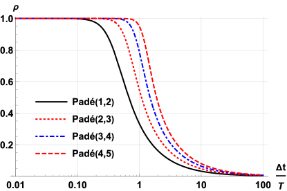
a= 0;

LogLinearPlot[{rho[1, 2, a, x], rho[2, 3, a, x], rho[3, 4, a, x], rho[4, 5, a, x]}, {x, 0.01, 100}, PlotRange -> {0, 1.01}]

Figure 3: Spectral radii of sub-diagonal Padé expansions ($M-1,M$).

The mixed-order Padé expansions are obtained in Eq. (23) with $0<\rho_{\infty}<1$ and $L<M$. It is identified from Eq. (20) that the highest orders of $P_{L/M}$ and $P_{M/M}$ are equal to $L$ and $M$, respectively, and the highest orders of $Q_{L/M}$ and $Q_{M/M}$ are both equal to $M$. The limit of the spectral radius as $\Delta t$ increases is obtained as

$$\lim_{\Delta t\rightarrow\infty}\left|\frac{\rho_{\infty}(\mathrm{i}2\pi\Delta t/T)^{M}+(1-\rho_{\infty})(\mathrm{i}2\pi\Delta t/T)^{L}}{\rho_{\infty}(\mathrm{i}2\pi\Delta t/T)^{M}+(1-\rho_{\infty})(\mathrm{i}2\pi\Delta t/T)^{M}}\right|=\rho_{\infty}\,.$$ (82)

It indeed tends to the specified $\rho_{\infty}$. As an example, the spectral radii of Padé expansions mixing the orders $(2,3)$ and $(3,3)$ are plotted in Fig. 4 at $\rho_{\infty}=1$, $0.75$, $0.5$, $0.25,$ and $0$. It is observed that the numerical dissipation is controlled by the specified value of $\rho_{\infty}$ over the range between $0$ and $1$. The spectral radius is strictly less than or equal to $1$.

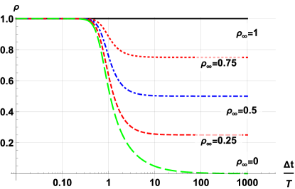
M = 3; L = M - 1;

LogLinearPlot[{rho[L, M, 1, x], rho[L, M, 3/4, x], rho[L, M, 1/2, x], rho[L, M, 1/4, x], rho[L, M, 0, x]}, {x, 0.01, 1000}, PlotRange -> {0, 1.01}]

Figure 4: Spectral radii of mixed-order Padé expansions with $L=2$ and $M=3$ at $\rho_{\infty}=1$, $0.75$, $0.5$, $0.25,$ and $0$.

The numerical dissipative characteristics of the proposed time-stepping schemes are compared with those of the HHT-$\alpha$ scheme for the cases of $\alpha=-0.05$, $\alpha=-0.1$, and $\alpha=-0.3$. In the high-frequency limit $\Delta t/T\rightarrow\infty$, the spectral radius tends to $\rho_{\infty}=0.90476$ at $\alpha=-0.05$, $\rho_{\infty}=0.81818$ at $\alpha=-0.1,$ and $\rho_{\infty}=0.53846$ at $\alpha=-0.3$. For each given value of $\alpha$, the corresponding value of $\rho_{\infty}$ is taken as an input in the proposed scheme. The spectral radii are compared in Fig. 5a for $\alpha=-0.05$, Fig. 5b for $\alpha=-0.1$, and Fig. 5c for $\alpha=-0.3$, respectively. The MATHEMATICA code is given with $\alpha=-0.05$, but it can be used for other values of $\rho_{\infty}$ (represented by the variable a) and $\alpha$. It is observed that the spectral radii of the proposed high-order scheme are closer to $1$ than the HHT-$\alpha$ scheme when the value of $\Delta t/T$ is small and decrease faster when the value of $\Delta t/T$ becomes large. This behaviour indicates that the proposed scheme is more accurate for lower modes and exhibits stronger numerical dissipation for higher modes.

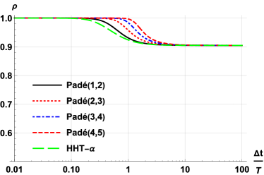
a) b)

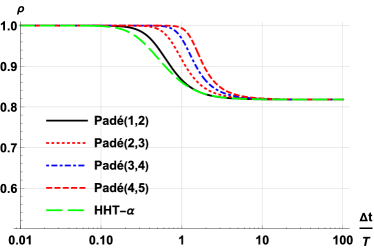
c)

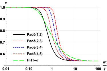
alpha = -0.05; a = (1 + alpha)/(1 - alpha);

LogLinearPlot[{rho[1, 2, a, x], rho[2, 3, a, x], rho[3, 4, a, x], rho[4, 5, a, x], HHTrho[alpha, x]}, {x, 0.01, 100}, PlotRange -> {0.5, 1.01}]

Figure 5: Spectral radii of mixed-order Padé expansions and HHT-$\alpha$ scheme for a) $\rho_{\infty}=0.90476$ at $\alpha=-0.05$, b) $\rho_{\infty}=0.81818$ at $\alpha=-0.1$, and c) $\rho_{\infty}=0.53846$ at $\alpha=-0.3$.

5.3 Period error

As it is observed by comparing the discrete-time solution in Eq. (62) with Eq. (66) to the continuous-time solution in Eq. (55), numerical errors arise not only from the amplitude but also from the phase of vibration. The exact solution of the phase $e^{\mathrm{i}2\pi\Delta t/T}$ is approximated by $e^{\mathrm{i}\bar{\Omega}}=R/\rho$ in the time-stepping scheme. The approximation $R/\rho$ of the proposed scheme with $\rho_{\infty}=0.53846$ and the HHT-$\alpha$ scheme with $\alpha=-0.3$ are compared to the exact solution in Fig. 6. It shows that the proposed high-order scheme is significantly more accurate than the HHT-$\alpha$ scheme. As the order increases, the accuracy of approximation improves rapidly.

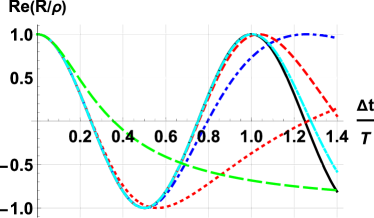
a) b)

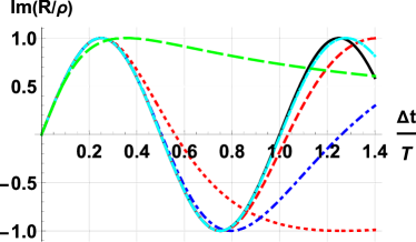
alpha = -0.3; a = (1 + alpha)/(1 - alpha);

Plot[{Re[Exp[2*Pi*x*I]], Re[ph[1, 2, a, x]], Re[ph[2, 3, a, x]], Re[ph[3, 4, a, x]], Re[ph[4, 5, a, x]], Re[HHTph[alpha, x]]}, {x, 0.0, 1.4}]

Figure 6: Phase of vibration of mixed-order Padé expansions at $\rho_{\infty}=0.53846$ and HHT-$\alpha$ with $\alpha=-0.3$: a) Real part, b) Imaginary part.

The relative period errors given by Eq. (72) for orders $(1,2)$, $(2,3)$, $(3,4)$, and $(4,5)$ of the mixed Padé scheme are plotted in Fig. 7 at two levels of numerical dissipation, together with those of the HHT-$\alpha$ scheme. The two levels of numerical dissipation are specified by $\rho_{\infty}=1$ and $\rho_{\infty}=0.53846$ corresponding to $\alpha=0$ and $\alpha=-0.3$, respectively. The relative period errors at $\rho_{\infty}=1$ are depicted by solid lines and those at $\rho_{\infty}=0.53846$ by dashed lines. It is observed that the relative period error decreases rapidly with the increase of the order of the scheme. As expected, introducing numerical dissipation leads to larger relative period errors since the order of accuracy of the Padé expansion is reduced by one.

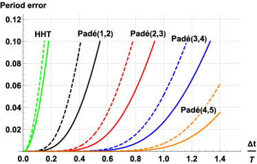
a1 = 1; a2 = 0; Plot[{pE[1, 2, a1, x], pE[1, 2, a2, x], pE[2, 3, a1, x], pE[2, 3, a2, x], pE[3, 4, a1, x], pE[3, 4, a2, x], pE[4, 5, a1, x], pE[4, 5, a2, x], HHTpE[0, x], HHTpE[-0.3, x]}, {x, 0.001, 1.4}, PlotRange -> {0, 0.1}]

Figure 7: Relative period errors. The present high-order scheme with $\rho_{\infty}=1$ and the HHT-$\alpha$ scheme with $\alpha=0$ are indicated by the solid lines and $\rho_{\infty}=0.53846$ and $\alpha=-0.3$ by the dashed lines.

5.4 Damping ratio

The damping ratios using the mixed-order Padé expansions are plotted in Fig. 8 as functions of $\Delta t/T$. The numerical damping is specified with $\rho_{\infty}=0.90476$ in Fig. 8a and $\rho_{\infty}=0.53846$ in Fig. 8b. It is found that the damping ratio tends to zero when the size of time step $\Delta t/T$ is small. This ensures that the effect of numerical damping on low-frequency modes is small.

a) b)

a = 0.90476;

Plot[{dR[1, 2, a, x], dR[2, 3, a, x], dR[3, 4, a, x], dR[4, 5, a, x]}, {x, 0.001, 1.4}, PlotRange -> {0, 0.1} ]

Figure 8: Damping ratios of mixed-order Padé expansions at: a) $\rho_{\infty}=0.90476$, b) $\rho_{\infty}=0.53846$.

5.5 Effect of the time step size on low-frequency modes

The choice of the time step size is critical in the effective use of numerical dissipation. To reduce the temporal discretization error, a small time step size is desirable. On the other hand, when the time step size is too small, vibrations of spurious high-frequency modes may not be sufficiently damped and pollute the solution. Therefore, it is necessary to choose a suitable time step size that will lead to the desired accuracy for the lower modes (below the maximum frequency of interest), and suppress the responses of the higher modes (above the maximum frequency of interest) at the same time. The effect of the time step size on the vibrations of lower modes is examined in this section in order to provide a guideline on the selection of the time step size.

The HHT-$\alpha$ scheme is one of the most widely used time integration methods in commercial software and in practice. It is addressed in Section 5.5.1 to provide a reference case for the discussion on the proposed high-order scheme in Section 5.5.2.

5.5.1 HHT-$\alpha$ scheme

The HHT-$\alpha$ scheme is of second-order accuracy. The amount of numerical dissipation is controlled by selecting the parameter $\alpha$ in the range of $0\geq\alpha\geq-1/3$. The period errors of $\alpha=0$, $-0.05$, $-0.1$, and $-0.3$ are shown in Fig. 9.

Plot[{HHTpE[0, x], HHTpE[-0.05, x], HHTpE[-0.1, x], HHTpE[-0.3, x]}, {x, 0.001, 0.1}, PlotRange -> {0, 0.05}]

Figure 9: Relative period error of HHT-$\alpha$ method with the parameter $\alpha=0$, $-0.05$, $-0.1$ and $-0.3$.

It is observed that numerical dissipation increases the relative period error. In the following, the case of $\alpha=-0.3$ is considered. In order to limit the error to $3\%$ at a given period $T$, the step size should not be larger than $\Delta t=0.08T$, i.e., about $12$ steps per period, which is a common choice in practice. To reduce the relative period error to $1\%$, the time increment must be below $\Delta t=0.04T$, which corresponds to 25 steps per period.

It is worthwhile to note that the error in the overall time integration also depends on the frequency contents of the excitation and will be smaller than the error at the maximum frequency of interest.

5.5.2 High-order scheme

It is shown in Section 5.2 that the proposed high-order scheme exhibits better properties of numerical dissipation than the HHT-$\alpha$ method in the range of $-0.05\geq\alpha\geq-0.3$ (i.e., $0.90476\geq\rho_{\infty}\geq 0.53846$). Parametric studies on the numerical examples in Section 6 demonstrate that spurious high-frequency oscillations can be effectively dissipated when the user-specified parameter is chosen between $0.90476\geq\rho_{\infty}\geq 0$. Only the case of $\rho_{\infty}=0.53846$, corresponding to $\alpha=-0.3$ in the HHT-$\alpha$ scheme, is considered in this section. When the value of $\rho_{\infty}$ is smaller, the effect of numerical dissipation on lower modes will be smaller at the same size of time step. Other cases such as the $L$-stable scheme ($\rho_{\infty}=0$) can be examined using the provided MATHEMATICA code.

Similar to the discussion on the HHT-$\alpha$ method, the relative period errors are shown in Fig. 10 for orders $(1,2)$, $(2,3)$, $(3,4)$, and $(4,5)$.

a = 0.53846;

LogLogPlot[{pE[1, 2, a, x], pE[2, 3, a, 2*x], pE[3, 4, a, 3*x], pE[4, 5, a, 4*x]}, {x, 0.05, 0.2}, PlotRange -> {10^(-8), 0.01}]

Figure 10: Relative period error of high-order scheme with $\rho_{\infty}=0.53846$ (corresponding to $\alpha=-0.3$ for HHT-$\alpha$ scheme). The MATHEMATICA commands are listed below the plots.

To summarize the observations and conclusions concisely, the order of the high-order scheme is denoted as $(L=M-1,M)$. Note that the time step size $\Delta t/T$ is scaled according to the order $L$ by a factor $1/L$ in the horizontal axis of the plot. For example, the period error of the order $(4,5)$ scheme with $L=4$ is found from Fig. 10 to be about $10^{-6}$ at $\Delta t/T=4\times 0.1=0.4$. It is noted that the relative period error of the high-order scheme is much smaller than that of the HHT-$\alpha$ scheme and should result in significantly higher accuracy.

6 Numerical examples

The dissipative and dispersive characteristics of the proposed scheme with controllable numerical damping have been analyzed using the free vibration of a single-degree-of-freedom problem in Section 5.5, where the selection of time step size is also discussed. In this section, the performance of solving a model problem with a high stiffness ratio is examined first. Wave propagation problems discretized with finite elements are then addressed. Finally, a simple guideline for the selection of $\rho_{\infty}$ and time step size $\Delta t$ is proposed for wave propagation problems.

We focus on evaluating the performance of the proposed scheme on the numerical dissipation of spurious high-frequency oscillations without affecting the low-frequency responses. Linear (1st-order) elements are utilized for the spatial discretization, which are known to lead to significant errors of spatially unresolved high-frequency modes in the semi-discretized equation of motion [9]. The use of high-order formulations to reduce the spatial discretization error is out of the scope of the present work and will be addressed in forthcoming publications.

The first five examples in this section are selected from the literature. The results obtained with the Bathe and other high-order methods are available in the cited references and can be directly used for comparison.

In our previous work [6], the convergence of the present method with respect to the time step size (and no numerical damping) has been studied. The computational times and accuracy are compared with the Newmark method, which has a similar computational cost to the HHT-$\alpha$ method. Since the difference in computer times taken by the present method with or without numerical dissipation is minor, the conclusions related to the computer times reached in [6] are still valid. As this paper focuses on the effectiveness of numerical dissipation, the evaluation of effectiveness and computer time in comparison with the HHT-$\alpha$ method is performed for given finite element models (semi-discretized systems). The evaluation is discussed in Section 6.6 on the large-scale simulation of a 3D sandwich panel.

Source codes of the proposed scheme written in MATLAB and FORTRAN are available for download at https://github.com/ChongminSong/HighOrderTimeIntegration. Interested readers may use the source codes to compare the computational cost and accuracy with other time-integration methods on their computer systems.

6.1 A three-degree-of-freedom model problem

The model problem studied in [18] and [28] is shown in Fig. 11. It consists of three masses connected by two springs with a high stiffness ratio. The spring and mass coefficients are given as $k_{1}=10^{7}$, $k_{1}=1$, $m_{1}=0$, $m_{2}=1$ and $m_{3}=1$. The displacement of $m_{1}$ is prescribed as

$$u_{1}=\sin\omega_{p}t$$ (83)

with $\omega_{p}=1.2$ corresponding to the period of vibration $T_{p}=5.236$. The equation of motion of the system is expressed

$$\left[\begin{array}[]{cc}m_{2}&0\\ 0&m_{3}\end{array}\right]\left\{\begin{array}[]{c}\ddot{u}_{2}\\ \ddot{u}_{3}\end{array}\right\}+\left[\begin{array}[]{cc}k_{1}+k_{2}&-k_{2}\\ -k_{2}&k_{2}\end{array}\right]\left\{\begin{array}[]{c}u_{2}\\ u_{3}\end{array}\right\}=\left\{\begin{array}[]{c}k_{1}u_{1}\\ 0\end{array}\right\}$$ (84)

with the displacements $u_{2}$ of $m_{2}$ and $u_{3}$ of $m_{3}$. The reaction force at $m_{1}$ is equal to

$$R_{1}=m_{1}\ddot{u}_{1}+k_{1}(u_{1}-u_{2})\,.$$ (85)

The system is initially at rest, $u_{2}(0)=\dot{u}_{2}(0)=u_{3}(0)=\dot{u}_{3}(0)=0$.

Figure 11: A three-degree-of-freedom model problem

Equation (84) can be solved by mode superposition. The two natural frequencies are approximately equal to $\omega_{1}=1$ and $\omega_{2}=3162$, which correspond to the periods of vibration $T_{1}=6.283$ and $T_{2}=0.002$. The reference solution is obtained by excluding the participation of the high-frequency mode $\omega_{2}$ from the mode superposition solution.

The time integration of the present high-order scheme is performed with the parameter $\rho_{\infty}=0$ and the time step size of $\Delta t=0.14$ as being used in [28]. This choice results in $\Delta t/T_{p}=0.0267$, $\Delta t/T_{1}=0.0223$ and $\Delta t/T_{2}=70.5$. Each period of excitation is divided into about 37 time steps. It is expected from Fig. 3 that the high-frequency oscillations with the period $T_{2}$ are rapidly damped. The analysis is performed for a long duration of $t=5000\approx 967T_{p}$.

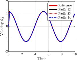
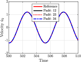
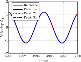
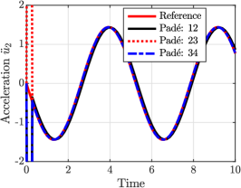
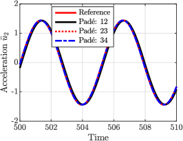
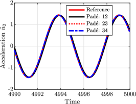
Figure 12: Velocity (top row) and acceleration (bottom row) responses of $m_{2}$ during $0\leq t\leq 10$ (left column), $500\leq t\leq 510$ (middle column) and $4900\leq t\leq 5000$ (right column).

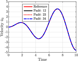
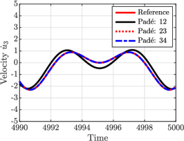
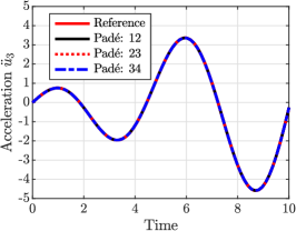
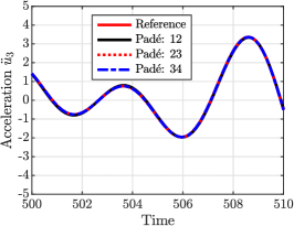
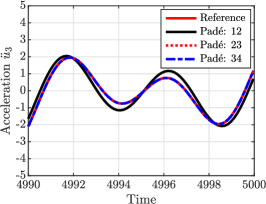
Figure 13: Velocity (top row) and acceleration (bottom row) responses of $m_{3}$ during $0\leq t\leq 10$ (left column), $500\leq t\leq 510$ (middle column) and $4900\leq t\leq 5000$ (right column).

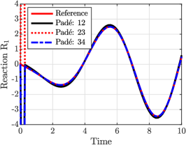
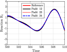
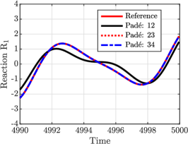
Figure 14: Reaction force response during $0\leq t\leq 10$ (left column), $500\leq t\leq 510$ (middle column) and $4900\leq t\leq 5000$ (right column).

Figures 12 and 13 show the velocity (in the top row) and acceleration (in the bottom row) responses of $m_{2}$ and $m_{3}$, respectively. The responses of the reaction force $R_{1}(t)$ are plotted in Fig. 14. The three columns of each figure show the responses at three different time intervals: $0\leq t\leq 10$ (left column), $500\leq t\leq 510$ (middle column) and $4900\leq t\leq 5000$ (right column). It is observed from Fig. 12 that the initial velocity $\dot{u}_{2}(0)=1$ is inconsistent with the initial condition ($\dot{u}_{2}(0)=0$) as the result of excluding the high-frequency vibrations. This inconsistency leads to a spike in the first time step of the acceleration $\ddot{u}_{2}$ in Fig. 12 and the reaction force $R_{1}$ in Fig. 14. After the first step, the result obtained at order $(1,2)$ differs slightly from the reference resolution. The increase of the difference with time (from the left column with $0\leq t\leq 10$ to the right column with $4900\leq t\leq 5000$) is appreciable in the responses of $m_{3}$ (Fig. 13) and reaction force $R_{1}$ (Fig. 14). The results obtained at orders $(2,3)$ and $(3,4)$ are indistinguishable from the reference solution throughout the whole duration, showing negligible numerical dissipation and phase error of the low-frequency mode. This example illustrates that high-order schemes are advantageous for analyses of long duration. The results reported in [18] using the Newmark method and [18, 28] using the Bathe method are available for comparison with the present results.

6.2 One-dimensional wave propagation in a homogeneous rod

The problem of elastic wave propagation in a one-dimensional prismatic rod, as sketched in Fig. 15, is frequently used in the literature when studying the numerical dissipation properties of time integration methods. The material and geometrical parameters are adopted from Ref. [33] with a consistent set of units: length of the rod $l=200,$ Young’s modulus $E=3\times 10^{7}$, Poisson’s ratio $\nu=0.0$, and mass density $\rho=0.00073$. The longitudinal wave speed is $c=\sqrt{E/\rho}=\sqrt{3\times 10^{7}/0.00073}=2.0272\times 10^{5}$. We assume that no physical damping is present. The left end of the rod is fixed and the right end is subjected to a step loading $pH(t)$ ($H(t)$ denotes the Heaviside function) with the amplitude of the pressure $p=10^{4}$. Since the step loading includes high-frequency components, it will excite some spurious high-frequency modes of the finite element model and therefore, numerical dissipation is desired.

Figure 15: A homogeneous elastic rod subjected to a step loading.

The effect of numerical dissipation on the response at a frequency (or a period $T$) depends on the time step size $\Delta t$. For a given mesh, the time step size is often expressed as the Courant-Friedrichs-Lewy (CFL) number defined in 1D as

$$\mathrm{CFL}=c\frac{\Delta t}{\Delta x}\,,$$ (86)

where $\Delta x$ denotes the element size. The CFL number measures the number of elements that the wave can travel in each time step. In a numerical analysis of wave propagation by direct time integration, the error mainly comes from two sources, the time discretization error controlled by the time step size $\Delta t$ and the spatial discretization error controlled by the element size $\Delta x$. For a wave with a period $T$, Eq. (86) can be rewritten as

$$\dfrac{cT}{\Delta x}=\mathrm{CFL}\dfrac{T}{\Delta t}\,.$$ (87)

It represents the ratio of the number of elements in one wavelength ($cT$) to the number of time steps in one period. Generally speaking, the CFL number reflects the relative amount of errors in time and spatial discretizations. In the remainder of this section, the selection of the weight factor $\rho_{\infty}$ and the CFL number for linear finite elements will be discussed.

6.2.1 Control of high-frequency numerical dissipation by $\rho_{\infty}$

The effect of the user-specified control parameter $\rho_{\infty}$ on the numerical dissipation is investigated in the following. The analysis is performed for a time duration of $0.02$. A uniform spatial discretization with 1,000 elements along the length (element size of $\Delta x=0.2$) is considered. The selection of the time step size (the CFL number for the given element size) will be discussed later in Section 6.2.2. In this section, the time step size for the order $(1,2)$ scheme is chosen to have a CFL number of $10$ leading to $\Delta t=9.8658\times 10^{-6}$, which means in each time step the wave travels through $10$ linear elements. Following the discussions in Section 5.5.2, the time step sizes of orders $(2,3)$, $(3,4)$ and $(4,5)$ are chosen by multiplying that of order $(1,2)$ with a factor of 2, 3 and 4, respectively, to introduce a similar amount of numerical dissipation. These time step sizes correspond to CFL numbers of 20 for order $(2,3)$, 30 for order $(3,4)$, and 40 for order $(4,5)$. In the subsequent analyses, the velocity at the middle point of the rod will be examined. For all the cases considered below, accurate results for displacement responses are obtained and will not be reported explicitly.

When the parameter $\rho_{\infty}=1$ (diagonal Padé expansions) is chosen, no numerical dissipation is introduced. The time histories of the dimensionless velocity $\rho cv/p$ at the middle of the rod are plotted in Fig. 16a versus the dimensionless time $ct/l$. In addition, the analytical solution is shown by the solid gray line. The peak value of the response is equal to $\rho cv/p=1$ for the analytical solution. A close-up view of the results from the dimensionless time $ct/l=16.3$ to $ct/l=17.7$ (corresponding to $t=0.016$ to $t=0.0175$) is depicted in Fig. 16b. Strong spurious high-frequency oscillations can be observed at all orders of the scheme. When $\rho_{\infty}=0$ is chosen, the scheme is $L-$stable and the maximum amount of numerical dissipation is introduced. The velocity responses are plotted in Fig. 17. It is observed that the high-frequency oscillations are largely suppressed by the addition of numerical dissipation.

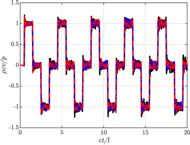
(a) Time histories.

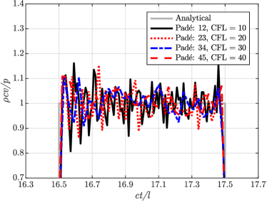
(b) Close-up view from $ct/l=16.3$ to $ct/l=17.7$.

Figure 16: Velocity responses at the middle point of 1D rod obtained by the high-order scheme with $\rho_{\infty}=1$.

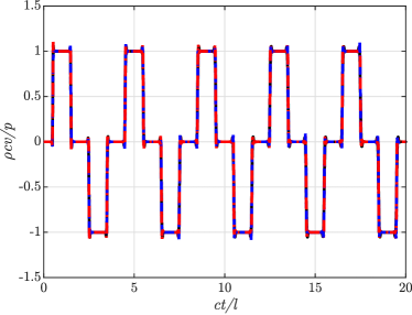
(a) Time histories.

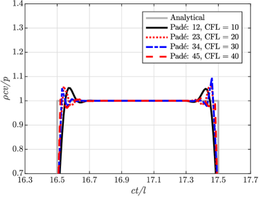
(b) Close-up view from $ct/l=16.3$ to $ct/l=17.7$.

Figure 17: Velocity responses at the middle point of 1D rod obtained by the high-order scheme with $\rho_{\infty}=0$.

The choice of the parameter $\rho_{\infty}$ is investigated by performing the analyses using three additional values of $\rho_{\infty}$ that correspond to typical values of the parameter $\alpha$ in the HHT-$\alpha$ method (For simplicity, we round the value $\rho_{\infty}$ to a single significant digit):

1. $\rho_{\infty}=0.9$, approximately corresponds to $\alpha=-0.05$ in the HHT-$\alpha$ method. This case is commonly regarded as lightly dissipative. The response histories of velocity at the middle of the rod are shown in Fig. 18.

2. $\rho_{\infty}=0.8$ corresponding to $\alpha=-0.1$. The response histories are shown in Fig. 19.

3. $\rho_{\infty}=0.5$ corresponding to $\alpha=-0.3$. This case is close to the maximum amount of numerical dissipation that can be introduced with the HHT-$\alpha$ method and is regarded as heavily dissipative. The velocity histories are shown in Fig. 20.

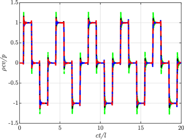
(a) Time histories

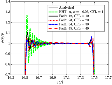
(b) Close-up view from $ct/l=16.3$ to $ct/l=17.7$.

Figure 18: Velocity responses at the middle point of 1D rod obtained by the proposed high-order scheme with $\rho_{\infty}=0.9$ and HHT-$\alpha$ method with $\alpha=-0.05$.

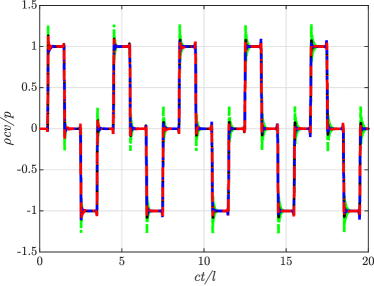
(a) Time histories.

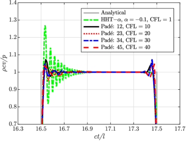
(b) Close-up view from $ct/l=16.3$ to $ct/l=17.7$.

Figure 19: Velocity responses at the middle point of 1D rod obtained by the proposed high-order scheme with $\rho_{\infty}=0.8$ and HHT-$\alpha$ method with $\alpha=-0.1$.

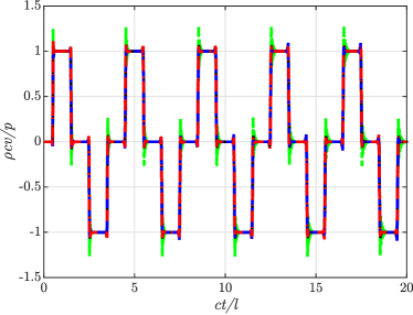
(a) Time histories.

(b) Close-up view from $ct/l=16.3$ to $ct/l=17.7$.

Figure 20: Velocity responses at the middle point of 1D rod obtained by the proposed high-order scheme with $\rho_{\infty}=0.5$ and HHT-$\alpha$ methods with $\alpha=-0.3$.

The results obtained with the HHT-$\alpha$ method at $\textrm{CFL}=1$ are also shown for comparison. It is observed that the proposed method at any order is able to suppress the spurious high-frequency oscillations. The duration and peak of spurious oscillations are smaller than those in the results obtained with HHT-$\alpha$ method. The effect of increasing the numerical dissipation by varying the parameter from $\rho_{\infty}=0.9$ to $\rho_{\infty}=0$ is minor. Therefore, $\rho_{\infty}$ can be selected from a rather wide range, say between $0.9$ and $0$, to effectively suppress spurious high-frequency oscillations. In the remainder of this section, a value of $\rho_{\infty}=0.8$ will be used as the controlling parameter for the high-order time-stepping scheme.

6.2.2 Effect of the time step size

When using a finite element model, the spatial discretization error, more specifically the highest frequency that can be accurately resolved by a given mesh, needs to be considered when choosing a suitable time step size. If $\Delta t$ is too small, spurious high-frequency oscillations will not be sufficiently damped. If $\Delta t$ is too large, low-frequency modes that can be accurately resolved by the mesh will be unnecessarily damped. As discussed previously, the time step size $\Delta t$ is represented by the CFL number. In the following, both a uniform mesh and non-uniform mesh are considered.

The analyses are performed using a uniform mesh consisting of $1{,}000$ elements for the orders $(1,2)$, $(2,3)$, $(3,4)$ and $(4,5)$. The parameter $\rho_{\infty}=0.8$ is chosen. The velocity response histories at the middle point of the rod are similar to those in Fig. 19. Therefore, only the close-up views of the response histories from $ct/l=16.3$ to $ct/l=17.7$ (i.e., $t=0.016$ to $t=0.0175$) are provided in Fig. 21. Following the observations made in Section 5.5.2, the CFL numbers are chosen according to the order of the scheme. Denoting the order as $(L=M-1,M)$, four different values of CFL number $5L$, $10L$, $15L$, and $20L$ are considered for each order $L=2$, $3$, $4,$ and $5$. It is observed by comparing Fig. 19b to Fig. 21 that all the CFL numbers lead to better results than that of the HHT-$\alpha$ method. The results corresponding to the lowest CFL number $5L$ show less than desirable numerical dissipation, while all the other CFL numbers lead to similar results. Therefore, the CFL numbers can be chosen from a rather wide range, and there are no obvious benefits in identifying optimal CFL numbers. In the remainder of this section, the CFL number is chosen as $10L$ for the order $(L=M-1,M)$ scheme. It is confirmed by a parametric study that this choice of the CFL number is also suitable for any value of $\rho_{\infty}$ between 0 and 1.

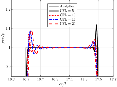
(a) Padé order $(1,2)$

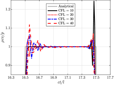
(b) Padé order $(2,3)$

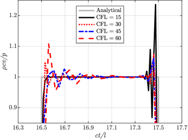
(c) Padé order $(3,4)$

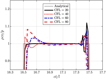
(d) Padé order $(4,5)$

Figure 21: Velocity responses at middle point of 1D rod obtained by the proposed high-order scheme at various CFL numbers with $\rho_{\infty}=0.8$.

In the next step, a non-uniform mesh is considered as often encountered in practical 2D or 3D finite element analyses. The coordinate $x_{i}$ of the node $i$ in a mesh of $n_{e}$ elements is given by

$$x_{i}=l\times\left(\frac{i-1}{n_{e}}+\dfrac{9}{11\times 20\pi}\sin^{2}\left(20\pi\frac{i-1}{n_{e}}\right)\right);\qquad(i=1,2,\ldots,n_{e}+1)\,.$$

The length of the elements varies as a sinusoidal function with a mean value of $l/n_{e}$ and a period of $l/20$. The length ratio of the largest element to the smallest element is about 10. The rod is divided into $n_{e}=2{,}000$ elements. The size of the largest and smallest element is equal to $9.088\times 10^{-4}l$ and $9.12\times 10^{-5}l$, respectively. Since the highest frequency that the mesh can accurately resolve is controlled by the largest elements, the time step size is chosen for the order $(L=M-1,M)$ scheme in such a way that the CFL number is about $10L$ according to the largest elements. This choice corresponds to a CFL number of $18L$ in terms of the average length of elements. The velocity response histories at the middle point of the rod are shown in Fig. 22. The spurious oscillations are largely suppressed by the proposed scheme. The result of the HHT-$\alpha$ method with $\alpha=-0.1$ and CFL$=1.8$ is also shown in the figures, in which strong oscillations are present.

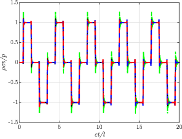
(a) Time histories.

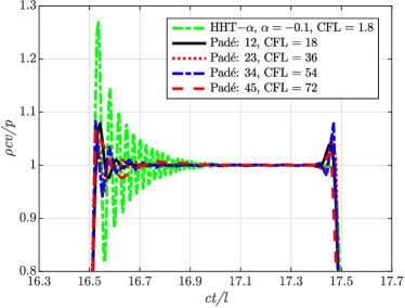
(b) Close-up view from from $ct/l=16.3$ to $ct/l=17.7$.

Figure 22: Velocity responses at the middle point of 1D rod obtained with a non-uniform mesh by the proposed high-order scheme with $\rho_{\infty}=0.8$ and HHT-$\alpha$ method with $\alpha=-0.1$. The CFL numbers shown are calculated using the average length of all elements.

6.3 One-dimensional wave propagation in a bi-material rod

The selection of $\rho_{\infty}$ and time step size $\Delta t$ is further evaluated using the bi-material rod (taken from Ref. [2]) shown in Fig. 23. The rod consists of two segments with a length of $2\,\mathrm{m}$ each. The wave speeds of the the left and right segments are equal to $c_{1}=40\sqrt{5}\,\mathrm{\,m/s}$ and $c_{2}=20\sqrt{2}\,\mathrm{\,m/s}$, respectively. The left end of the rod is fixed. A traction of $p=1\,\mathrm{Pa}$ is applied as a step function to the right end.

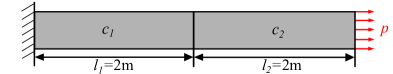
Figure 23: A bi-material rod subjected to a step loading.

For the subsequent analyses, a uniform mesh is used, where each segment is divided into $1{,}000$ linear finite elements. Since the wave travels within a time step through fewer elements in the right segment with a lower speed than in the left segment, the spatial discretization error is relatively higher. Thus, the time step size is determined from the CFL numbers of the right segment chosen as $\mathrm{CFL}=10L$ for the $(L=M-1,M)$ order scheme. The parameter $\rho_{\infty}=0.8$ is adopted. The velocity and axial-stress response histories at the interface of the materials (i.e., the middle point of the rod) are plotted in Figs. 24a and 25a, respectively. The results obtained using the HHT-$\alpha$ method with corresponding $\alpha=-0.1$ and $\mathrm{CFL}=1$ are shown in Figs. 24b and 25b for comparison. It is observed that the proposed scheme is more effective in suppressing spurious high-frequency oscillations. The results obtained with the Bathe method and an overlapping finite element scheme are reported in Ref. [2].

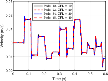
(a) Proposed high-order scheme with $\rho_{\infty}=0.8$.

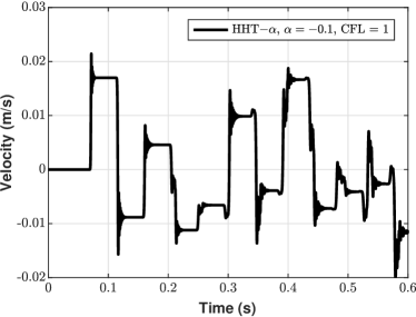
(b) HHT-$\alpha$ method with $\alpha=-0.1$.

Figure 24: Velocity responses at middle point of 1D bi-material rod. The CFL numbers shown are calculated using the lower wave speed.

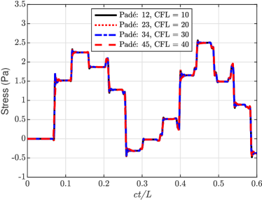
(a) Proposed high-order scheme with $\rho_{\infty}=0.8$.

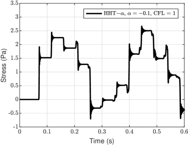
(b) HHT-$\alpha$ method with $\alpha=-0.1$.

Figure 25: Axial stress responses at middle point of 1D bi-material rod. The CFL numbers shown are calculated using the lower wave speed.

6.4 Scalar wave propagation in a square domain

The problem of scalar wave propagation in a square domain [24] is shown in Fig. 26. The edges of the square domain of dimension $l\times l$ are fixed. The wave speed is denoted as $c$. An initial velocity $A$ is prescribed over an area of $0.5l\times 0.5l$ (shaded square in Fig. 26) at the middle of the domain.

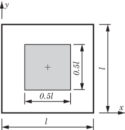
Figure 26: Scalar wave propagation in a square domain.

The analytical solutions for the displacement and velocity responses are obtained by the method of separation of variables as

$$u(x,y,t) =\dfrac{16A}{\pi^{2}}\sum_{m=1}^{\infty}\sum_{n=1}^{\infty}\dfrac{1}{mn}\dfrac{1}{\mu_{mn}}\sin(\mu_{mn}t)\sin\frac{m\pi}{2}\sin\frac{m\pi}{4}\sin\frac{n\pi}{2}\sin\frac{n\pi}{4}\sin\frac{m\pi x}{l}\sin\frac{n\pi y}{l}\,,$$ (88a)

$$\dot{u}(x,y,t) =\dfrac{16A}{\pi^{2}}\sum_{m=1}^{\infty}\sum_{n=1}^{\infty}\dfrac{1}{mn}\cos(\mu_{mn}t)\sin\frac{m\pi}{2}\sin\frac{m\pi}{4}\sin\frac{n\pi}{2}\sin\frac{n\pi}{4}\sin\frac{m\pi x}{l}\sin\frac{n\pi y}{l}\,,$$ (88b)

with

$$\mu_{mn}=\frac{c\pi}{l}\sqrt{m^{2}+n^{2}}\,.$$ (89)

In the following analyses, $l=1\,\,\mathrm{m}$, $c=1\,\mathrm{\,m/s}$, and $A=1\,\mathrm{\,m/s}$ are chosen. Considering symmetry, only a quarter of the domain ($0.5l\leq x\leq l$, $0.5l\leq y\leq l$) is modeled. A mesh of $1000\times 1000$ linear finite elements is generated. The parameter $\rho_{\infty}=0.8$ is used to introduce numerical dissipation. The CFL number is calculated using Eq. (86), where $\Delta x$ is chosen as the length of a finite element equal to $\Delta x=5\times 10^{-4}l.$ The time step size is determined to attain $\mathrm{CFL}=10L$ for the $(L=M-1,M)$ order scheme. The velocity response histories at the center of the square domain, indicated by a cross in Fig. 26, are plotted in Fig. 27a together with the analytical solution. The results of HHT-$\alpha$ method with $\alpha=-0.1$ and $\mathrm{CFL}=1$ are shown Fig. 28. It is again observed that the proposed high-order scheme is more effective in dissipating spurious high-frequency oscillations. Results for this example obtained with a high-order method are reported in Ref. [24].

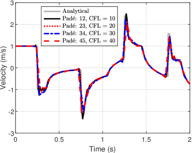
(a) Proposed high-order scheme with $\rho_{\infty}=0.8$.

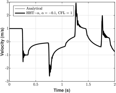
Figure 27: HHT-$\alpha$ method with $\alpha=-0.1$.

Figure 28: Velocity responses at center of square domain.

6.5 Two-dimensional wave propagation in a semi-infinite elastic domain - Lamb problem

Lamb’s problem with a vertical point load is analyzed in this section. The square domain of dimension $l\times l$ representing the semi-infinite elastic plane and boundary conditions are depicted in Fig. 29. Due to symmetry, only the right side to the point load $F(t)$ is considered. The geometry and materials parameters presented in Refs. [2] and [34] are adopted: Length of the square domain $l=3{,}200\,\mathrm{\,m},$ Young’s modulus $E=18.77\times 10^{9}\,\mathrm{\,Pa},$ Poisson’s ratio $\nu=0.25$, and mass density $\rho=2{,}200\,\mathrm{\,kg/m^{3}}$. Plane strain conditions are assumed. The P-wave, S-wave and Rayleigh-wave velocities are equal to $c_{p}=3{,}200\,\,\mathrm{m/s}$, $c_{s}=1{,}847.5\,\mathrm{\,m/s}$, and $c_{R}=1{,}698.6\,\,\mathrm{m/s}$, respectively. The time history of the point load consists of three step functions: $F(t)=2\times 10^{6}(H(0.15-t)-3H(0.1-t)+3H(0.05-t))\,\mathrm{N}$. The analytical solution of the horizontal and vertical displacements at the two points, $P_{1}\,(640,3{,}200)$ and $P_{2}\,(1{,}280,3{,}200)$, indicated in Fig. 29 are given in [2] until $t=1\,\,\mathrm{s},$ when the P-waves reach the right side of the domain.

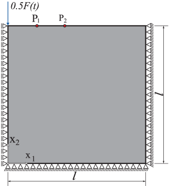
Figure 29: A semi-infinite elastic domain in plane strain conditions

The square domain is divided into a uniform mesh of $2{,}000\times 2{,}000$ linear finite elements. The side length $\Delta x$ of each square element is $1.6\,\mathrm{m}$. In the calculation of the CFL number, the P-wave velocity $c_{p}$ and side length $\Delta x$ are used.

An analysis using the HHT-$\alpha$ method with $\alpha=-0.1$ and $\mathrm{CFL=1}$ is also performed. The displacements and velocity responses are plotted in Figs. 30 and 31, respectively. The peak responses of vertical displacements are about 5 times larger than those of horizontal displacements. The displacements show good agreement with the analytical solution. Some spurious oscillations of the smaller horizontal displacements are observed. However, the velocity responses in Fig. 31 exhibit very strong high-frequency oscillations. The presence of waves traveling at different speeds renders the numerical dissipation of the HHT-$\alpha$ method much less effective than in the example of scalar waves (Section 6.4). The displacement responses obtained with the Bathe method are available in [2] and [34] for comparison.

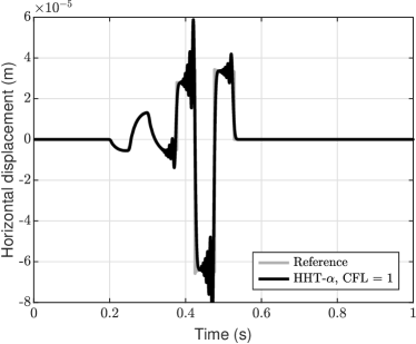
(a) Horizontal displacement at $P_{1}$

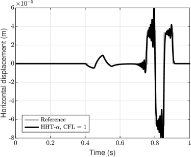
(b) Horizontal displacement at $P_{2}$

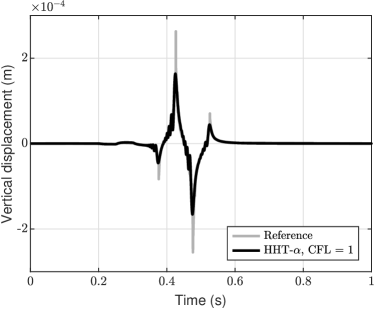
(c) Vertical displacement at $P_{1}$

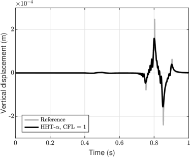
(d) Vertical displacement at $P_{2}$

Figure 30: Horizontal and vertical displacements of an semi-infinite elastic domain obtained by HHT-$\alpha$ method.

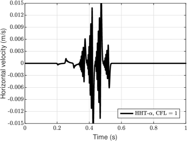
(a) Horizontal velocity at $P_{1}$

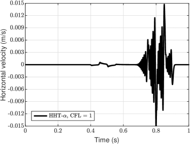
(b) Horizontal velocity at $P_{2}$

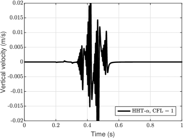
(c) Vertical velocity at $P_{1}$

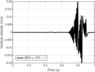
(d) Vertical velocity at $P_{2}$

Figure 31: Horizontal and vertical velocities of a semi-infinite elastic domain obtained by HHT-$\alpha$ method.

In the analysis using the high-order scheme, the parameter $\rho_{\infty}=0.8$ is adopted to introduce numerical dissipation. The CFL numbers for the time-integration scheme at orders $(1,2)$, $(2,3)$ and $(3,4)$ are selected as $10$, $20$ and $30$, respectively. Correspondingly, the time step sizes are given by $\Delta t=\Delta x\times\mathrm{CFL}/c_{p}$ as $0.005\,\mathrm{s}$, $0.01\,\mathrm{s}$ and $0.015\,\mathrm{s}$. The displacement and velocity responses are plotted in Fig. 32 and Fig. 33, respectively. Very good agreement of the displacement response with the analytical solution is observed. Spurious oscillations in the velocity response are largely suppressed.

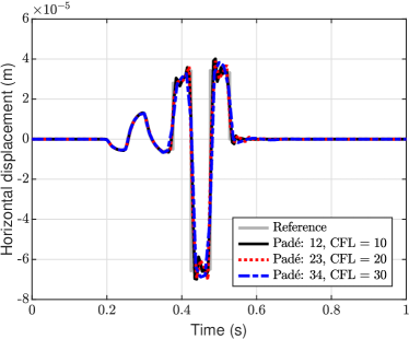
(a) Horizontal displacement at $P_{1}$

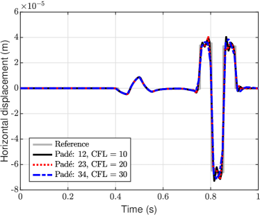
(b) Horizontal displacement at $P_{2}$

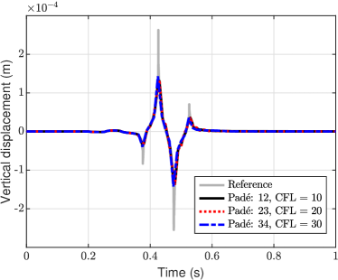
(c) Vertical displacement at $P_{1}$

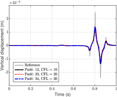
(d) Vertical displacement at $P_{2}$

Figure 32: Horizontal and vertical displacements of a semi-infinite elastic domain obtained by the proposed high-order scheme.

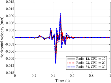
(a) Horizontal velocity at $P_{1}$

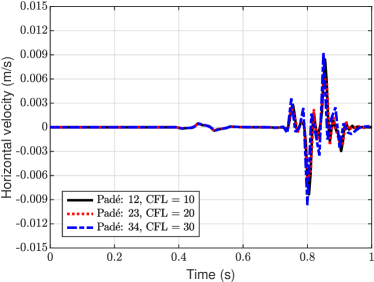
(b) Horizontal velocity at $P_{2}$

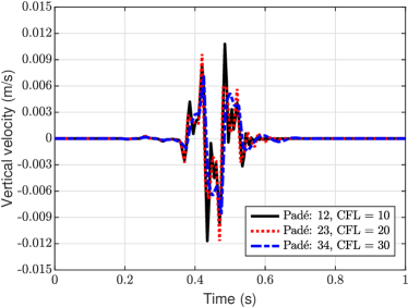
(c) Vertical velocity at $P_{1}$

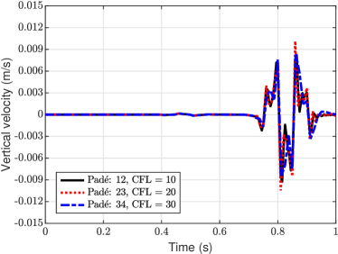
(d) Vertical velocity at $P_{2}$

Figure 33: Horizontal and vertical velocities of the Lamb problem obtained by the proposed high-order scheme.

6.6 Three-dimensional wave propagation in 3D sandwich panel

A sandwich panel with two cover-sheets and a foam-core is shown in Fig. 34a. The outer dimension of the panel is $288\,\mathrm{mm}\times 72\,\mathrm{mm}\times 59.5\,\mathrm{mm}$ and the thickness of the cover sheets is $5.76\,\mathrm{mm}$. The cover-sheets are made of steel with the following properties: Young’s modulus $E_{\mathrm{s}}=210\,\mathrm{GPa}$, Poisson’s ratio $\nu_{\mathrm{s}}=0.3$, and the mass density $\rho_{\mathrm{s}}=8050\,\nicefrac{\mathrm{kg}}{\mathrm{m^{3}}}$. Therefore, the P- and S-wave speeds are $c_{p}=5926\,\mathrm{m/s}$ and $c_{s}=3168\,\mathrm{m/s}$, respectively. The foam-core is given as a digital image obtained by X-ray CT scans. The material of the foam is aluminium with the property $E_{\mathrm{a}}=70\,\mathrm{GPa}$, $\nu_{\mathrm{a}}=0.3$ and $\rho_{\mathrm{a}}=2700\,\mathrm{kg/m^{3}}$. The corresponding wave speeds are $c_{p}=6198\,\mathrm{m/s}$ and $c_{s}=3122\,\mathrm{m/s}$, respectively. The right end of the panel is fixed in the normal direction and the left end of the top cover-sheet is subjected to a uniformly distributed pressure $p(t)$. The time history of the pressure consists of two step functions: $p(t)=1\times(2H(1.5\times 10^{-5}-t)-H(3\times 10^{-5}-t))\,\mathrm{kPa}$.

The sandwich panel is discretized by an octree mesh as shown in Fig. 34b and modelled by the scaled boundary finite element method [11, 35]. The smallest and largest element sizes are $0.48\,\mathrm{mm}$ and $1.92\,\mathrm{mm}$, respectively. Overall, the mesh consists of 597,325 elements, 1,099,242 nodes, and consequently, 3,297,726 degrees of freedom.

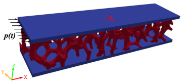
(a) Geometry

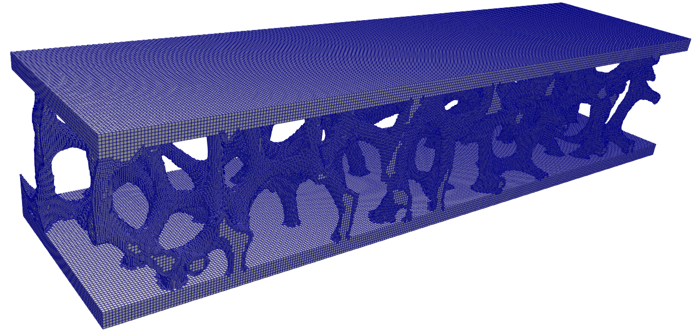
(b) Octree mesh

Figure 34: Sandwich panel.

The time integration using the proposed high-order schemes is performed with the parameter $\rho_{\infty}=0.8$ to suppress the oscillations in the response due to the high-frequency components in the excitation. The time step size is selected based on the CFL number in the steel cover-plates, where the element size is $0.96\,\mathrm{mm}$. The simulation is performed until $t_{\mathrm{sim}}=6\times 10^{-4}\,{\textstyle\mathrm{s}}$, which allows the waves to be reflected at the two ends for several times. As for the examples in the previous sections, the CFL number is chosen as 10 for order (1,2) and 20 for order (2,3). The corresponding time step size is equal to $\Delta t=1.5\times 10^{-6}\,{\textstyle\mathrm{s}}$ for order (1,2), resulting in 400 time steps, and $\Delta t=3\times 10^{-6}\,{\textstyle\mathrm{s}}$ for order (2,3) with 200 time steps.

The displacement and velocity responses along the $x-$direction at the middle point of the top surface $\mathrm{A}\!\left(144,36,57.6\right)$ (unit: mm), indicated by the red dot in Fig. 34a, are plotted in Fig. 35a and Fig. 35b, respectively. The black solid line and red dotted line represent the responses obtained using the proposed scheme at orders (1,2) and (2,3), respectively. The results are nearly identical to each other. An analysis using HHT-$\alpha$ method with $\alpha=-0.1$ and CFL = 1 (with $\Delta t=0.15\times 10^{-6}\,{\textstyle\mathrm{s}}$ and $4,000$ time steps) is also performed. The result is indicated by the green dashed line. The displacement response in Fig. 35a is in very good agreement with those of the proposed scheme, but the velocity in Fig. 35b shows strong spurious oscillations.

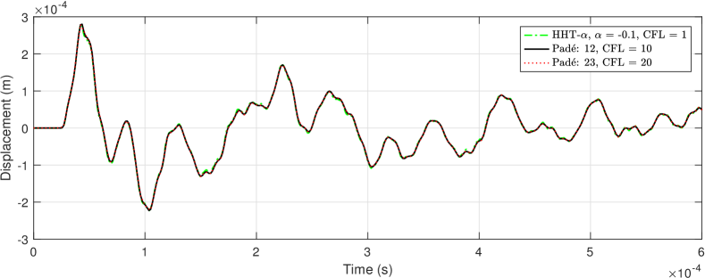
(a) Displacement in $x-$direction

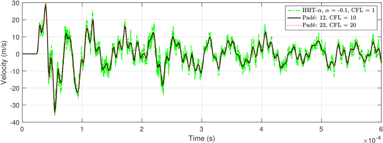
(b) Velocity in $x-$direction

Figure 35: Responses of sandwich panel at point $\mathrm{A}$ obtained by the proposed high-order scheme with $\rho_{\infty}=0.8$ and HHT-$\alpha$ method with $\alpha=-0.1$.

The contours of velocity along the $x-$direction at six selected time instances are presented in Fig. 36. The waves initially concentrate in the upper cover-plate, and gradually excite the lower cover-plate through the foam core.

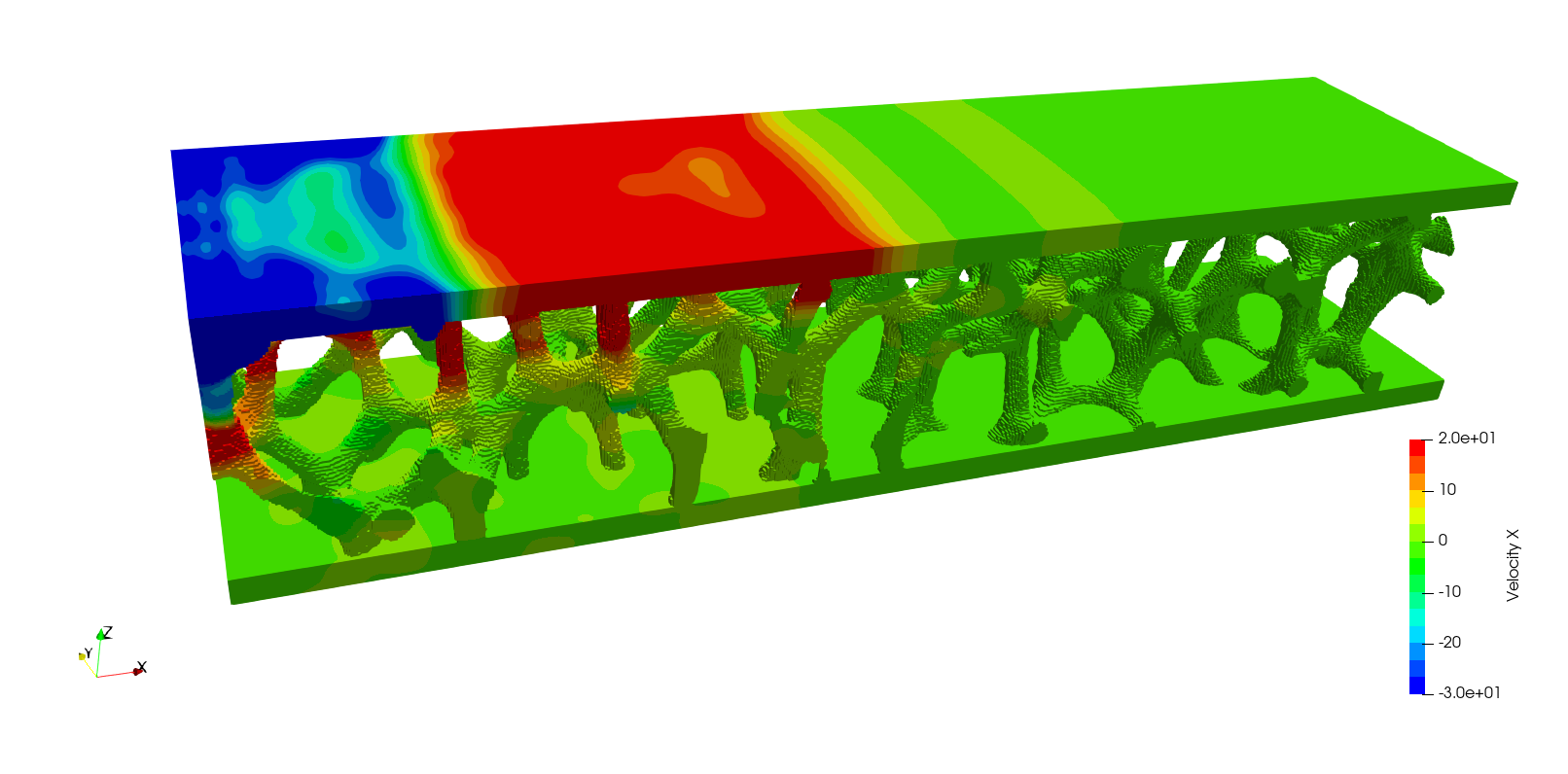
(a) $t=2.4\times 10^{-5}\,{\textstyle\mathrm{s}}$

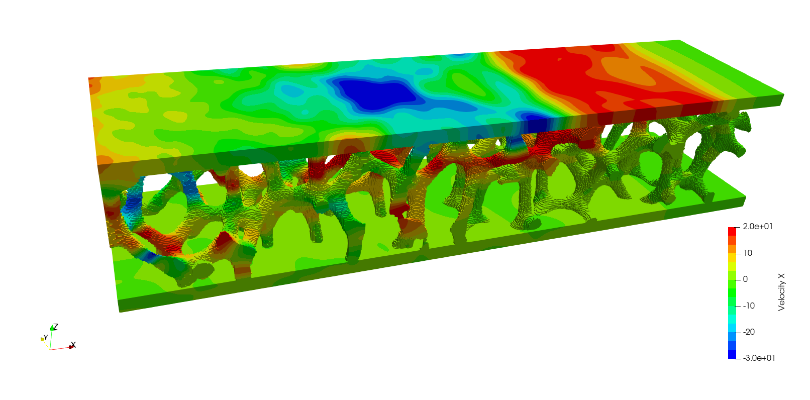
(b) $t=4.8\times 10^{-5}\,{\textstyle\mathrm{s}}$

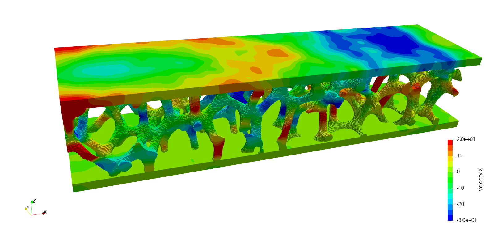
(c) $t=7.2\times 10^{-5}\,{\textstyle\mathrm{s}}$

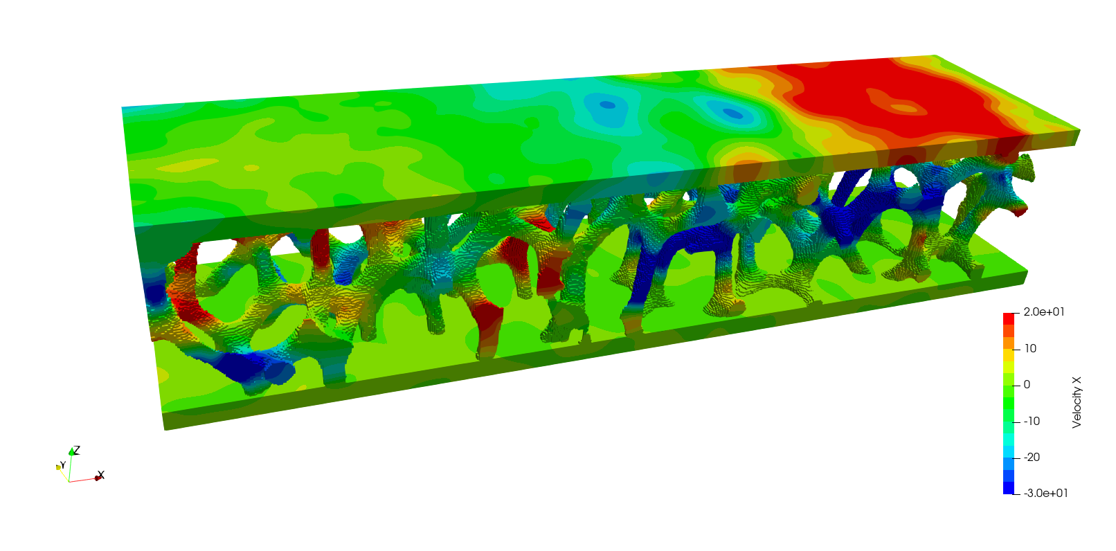
(d) $t=9.6\times 10^{-5}\,{\textstyle\mathrm{s}}$

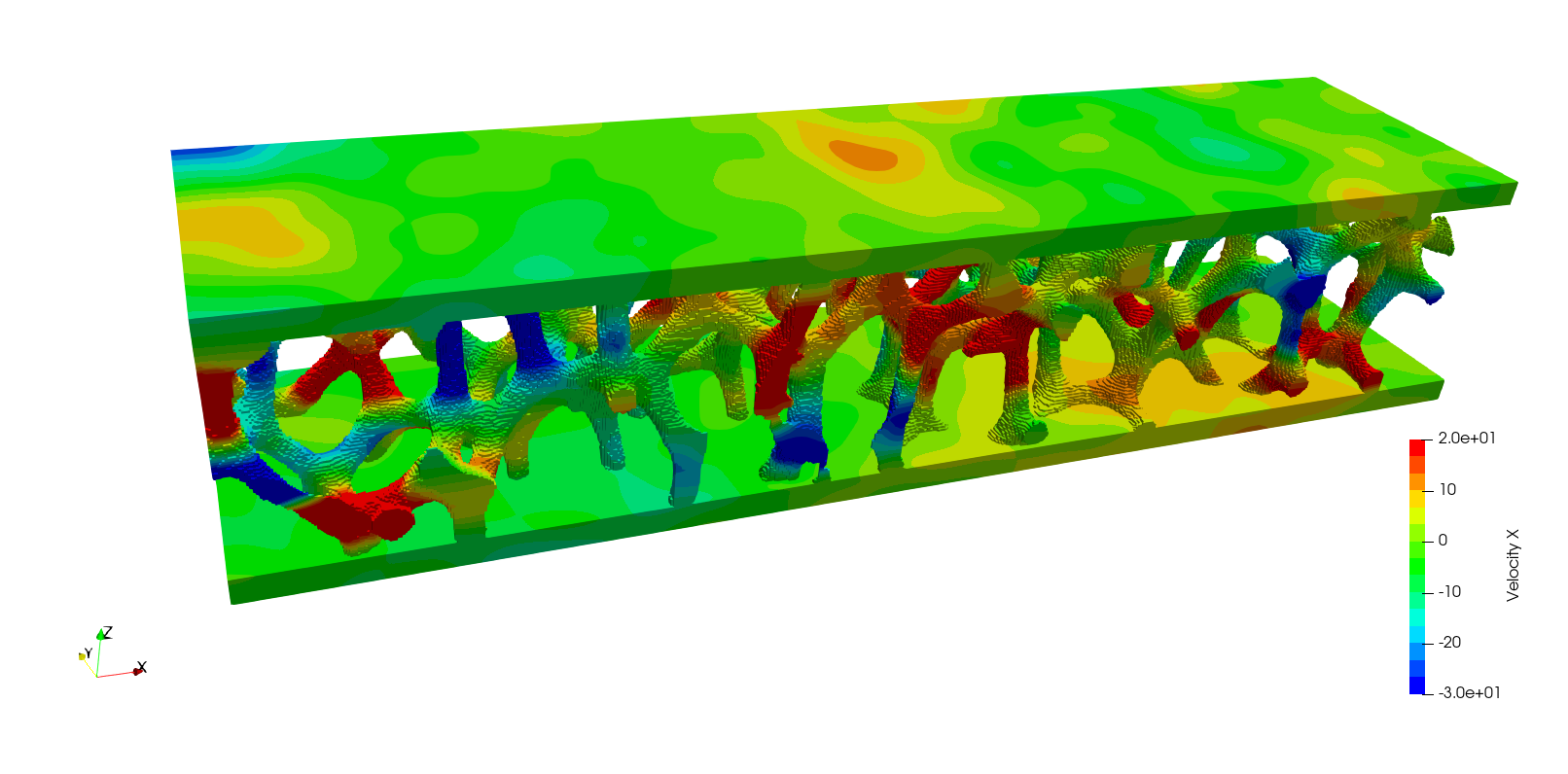
(e) $t=3.14\times 10^{-4}\,{\textstyle\mathrm{s}}$

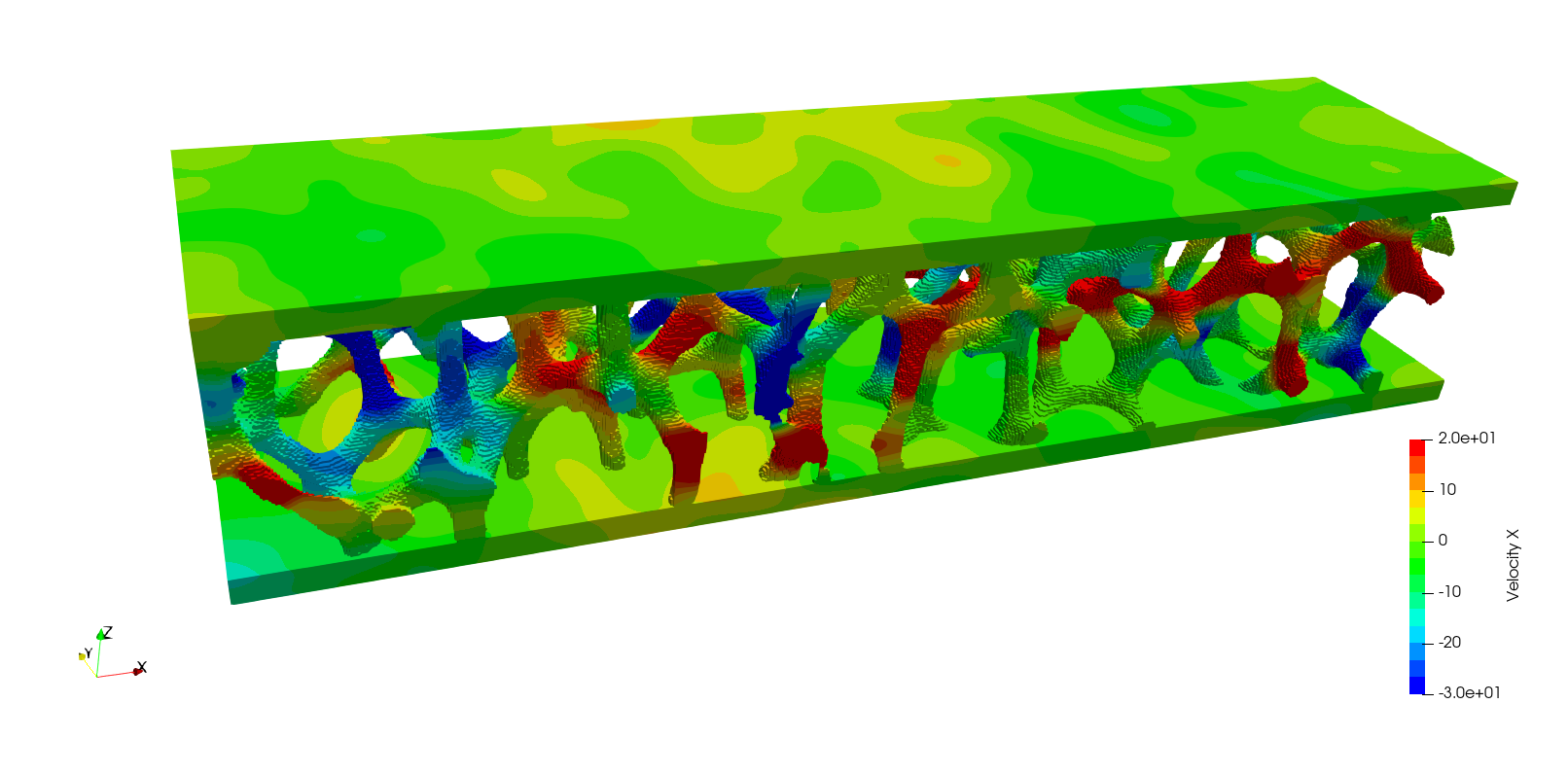
(f) $t=5.84\times 10^{-4}\,{\textstyle\mathrm{s}}$

Figure 36: Contours of velocity along the $x-$direction of sandwich panel at various time instances

The computational costs of the proposed scheme are evaluated for this example. The computer program for time integration is written in FORTRAN. The PARDISO direct solver of Intel’s Math Kernel Library (MKL) is employed for the solution of simultaneous linear algebraic equations (Eq. (35) for a real root and Eq. (40) for a complex root). This operation takes the majority of the running time. For this example of elasto-dynamics, the factorization of matrices is performed once at the beginning of the analysis. Only back-substitutions are performed during the time stepping. The computer running times are measured on a Dell Precision 5820 Tower Workstation with an Intel(R) Xeon(R) W-2275 CPU and 256 GB RAM. The HHT-$\alpha$ method takes 4,007 s for time stepping. The proposed scheme takes 960 s at order (1,2) and 857 s at order (2,3), which corresponds to speedup factors of about 4.18 and 4.69, respectively, in comparison with the HHT-$\alpha$ method.

7 Conclusions

A high-order implicit time integration scheme is proposed. The amount of numerical dissipation is controlled by using the spectral radius $\rho_{\infty}$ at the high-frequency limit as a user-specified parameter. The scheme varies with the specified parameter from A-stable (without numerical dissipation) to L-stable (with the maximum amount of numerical dissipation). The numerical dissipation is minimal at the low-frequency range and rapidly approaches the maximum value at the high-frequency range, showing better characteristics than the second-order HHT-$\alpha$ method. Moreover, the period error is smaller in the low-frequency range than that of the HHT-$\alpha$ method by orders of magnitude.

From the viewpoint of application, the only user-specified parameters are the value of the spectral radius in the high-frequency limit, $\rho_{\infty}$, and the time step size, $\Delta t$, expressed in terms of the CFL number. Effective dissipation of spurious high-frequency oscillations can be achieved in a wide range of the parameters: $0\leq\rho_{\infty}\leq 0.9$ and $5L\leq\mathrm{\textrm{CFL}}\leq 20L$ for a scheme of order $(L=M-1,M)$ when finite elements of linear shape functions are used for spatial discretization. The values $\rho_{\infty}=0.8$ and $\mathrm{\textrm{CFL}}=10L$ are used for wave propagation problems in this paper.

An efficient numerical algorithm is designed, where the systems of equations to be solved are similar in complexity to those in the standard Newmark method. Existing computer codes of the Newmark, HHT-$\alpha$, and generalize-$\alpha$ methods can be extended straightforwardly to include the proposed high-order scheme. When compared with the HHT-$\alpha$ method for the same finite element model, the proposed scheme is not only more effective in dissipating spurious high-frequency oscillations but also reduces computer running time. A speedup factor of more than 4 is observed when solving the sandwich panel problem employing our FORTRAN code with the Intel MKL PARDISO direct solver.

References

- [1] D. M. Hernandez, S. Hadden, J. Makino, Are long-term N-body simulations reliable?, Monthly Notices of the Royal Astronomical Society 493 (2) (2020) 1913–1925. doi:10.1093/mnras/staa388.
- [2] K. T. Kim, K. J. Bathe, Accurate solution of wave propagation problems in elasticity, Computers & Structures 249 (2021) 106502. doi:10.1016/j.compstruc.2021.106502.
- [3] Q. Gao, C. B. Nie, An accurate and efficient Chebyshev expansion method for large-scale transient heat conduction problems, Computers & Structures 249 (2021) 106513. doi:10.1016/j.compstruc.2021.106513.
- [4] K. J. Bathe, M. M. I. Baig, On a composite implicit time integration procedure for nonlinear dynamics, Computers & Structures 83 (31-32) (2005) 2513–2524. doi:10.1016/j.compstruc.2005.08.001.
- [5] O. C. Zienkiewicz, R. L. Taylor, J. Z. Zhu, The finite element method: its basis and fundamentals, 6th Edition, Elsevier Butterworth-Heinemann, 2005.
- [6] C. Song, S. Eisenträger, X. Zhang, High-order implicit time integration scheme based on Padé expansions, Computer Methods in Applied Mechanics and Engineering 390 (2022) 114436. doi:10.1016/j.cma.2021.114436.
- [7] K. J. Bathe, Finite element procedures, 2nd Edition, Prentice Hall, Pearson Education, Inc., 2014.
- [8] S. Duczek, H. Gravenkamp, Mass lumping techniques in the spectral element method: On the equivalence of the row-sum, nodal quadrature, and diagonal scaling methods, Computer Methods in Applied Mechanics and Engineering 353 (2019) 516–569. doi:10.1016/j.cma.2019.05.016.
- [9] J. A. Cottrell, A. Reali, Y. Bazilevs, T. J. R. Hughes, Isogeometric analysis of structural vibrations, Computer Methods in Applied Mechanics and Engineering 195 (41-43) (2006) 5257–5296. doi:10.1016/j.cma.2005.09.027.
- [10] C. Song, The scaled boundary finite element method in structural dynamics, International Journal for Numerical Methods in Engineering 77 (8) (2009) 1139–1171. doi:10.1002/nme.2454.
- [11] C. Song, The scaled boundary finite element method: Introduction to theory and implementation, Wiley, 2018. doi:10.1002/9781119388487.
- [12] J. C. Houbolt, A recurrence matrix solution for the dynamic response of elastic aircraft, Journal of the Aeronautical Sciences 17 (9) (1950) 540–550. doi:10.2514/8.1722.
- [13] N. M. Newmark, A method of computation for structural dynamics, ASCE Journal of the Engineering Mechanics Division 85 (3) (1959) 2067–2094. doi:10.1061/JMCEA3.0000098.
- [14] E. L. Wilson, I. Farhoomand, K. J. Bathe, Nonlinear dynamic analysis of complex structures, Earthquake Engineering and Structural Dynamics 1 (3) (1972) 241–252. doi:10.1002/eqe.4290010305.
- [15] H. M. Hilber, T. J. R. Hughes, R. L. Taylor, Improved numerical dissipation for time integration algorithms in structural dynamics, Earthquake Engineering and Structural Dynamics 5 (3) (1977) 283–292. doi:10.1002/eqe.4290050306.
- [16] J. Chung, G. M. Hulbert, A time integration algorithm for structural dynamics with improved numerical dissipation: the generalized- method, Journal of Applied Mechanics 60 (2) (1993) 371–375. doi:10.1115/1.2900803.
- [17] K. J. Bathe, Conserving energy and momentum in nonlinear dynamics: a simple implicit time integration scheme, Computers & Structures 85 (7-8) (2007) 437–445. doi:10.1016/j.compstruc.2006.09.004.
- [18] G. Noh, K. J. Bathe, Further insights into an implicit time integration scheme for structural dynamics, Computers & Structures 202 (2018) 15–24. doi:10.1016/j.compstruc.2018.02.007.
- [19] M. M. Malakiyeh, S. Shojaee, S. Hamzehei-Javaran, K. J. Bathe, New insights into the 1/2-Bathe time integration scheme when L-stable, Computers & Structures 245 (2021) 106433. doi:10.1016/j.compstruc.2020.106433.
- [20] W. Kim, J. N. Reddy, A new family of higher-order time integration algorithms for the analysis of structural dynamics, Journal of Applied Mechanics 84 (7) (2017) 071008. doi:10.1115/1.4036821.
- [21] W. Kim, J. N. Reddy, Effective higher-order time integration algorithms for the analysis of linear structural dynamics, Journal of Applied Mechanics 84 (7) (2017) 071009. doi:10.1115/1.4036822.
- [22] W. Kim, S. Y. Choi, An improved implicit time integration algorithm: The generalized composite time integration algorithm, Computers & Structures 196 (2018) 341–354. doi:10.1016/j.compstruc.2017.10.002.
- [23] W. Kim, J. H. Lee, A comparative study of two families of higher-order accurate time integration algorithms, International Journal of Computational Methods 17 (08) (2020) 1950048. doi:10.1142/S0219876219500488.
- [24] D. Soares, A straightforward high-order accurate time-marching procedure for dynamic analyses, Engineering with Computers 38 (2020) 1659–1677. doi:10.1007/s00366-020-01129-1.
- [25] P. Behnoudfar, Q. Deng, V. M. Calo, High-order generalized- method, Applications in Engineering Science 4 (2020) 100021. doi:10.1016/j.apples.2020.100021.
- [26] P. Behnoudfar, Q. Deng, V. M. Calo, Higher-order generalized- methods for hyperbolic problems, Computer Methods in Applied Mechanics and Engineering 378 (2021) 113725. doi:10.1016/j.cma.2021.113725.
- [27] S.-B. Kwon, K.-J. Bathe, G. Noh, Selecting the load at the intermediate time point of the -bathe time integration scheme, Computers & Structures 254 (2021) 106559. doi:10.1016/j.compstruc.2021.106559.
- [28] B. Choi, K.-J. Bathe, G. Noh, Time splitting ratio in the -bathe time integration method for higher-order accuracy in structural dynamics and heat transfer, Computers & Structures 270 (2022) 106814. doi:10.1016/j.compstruc.2022.106814.
- [29] M. F. Reusch, L. Ratzan, N. Pomphrey, W. Park, Diagonal Padé approximations for initial value problems, SIAM journal on scientific and statistical computing 9 (5) (1988) 829–838. doi:10.1137/0909055.
- [30] M. Wang, F. T. K. Au, Precise integration method without inverse matrix calculation for structural dynamic equations, Earthquake Engineering and Engineering Vibration 6 (2007) 57–64. doi:10.1007/s11803-007-0661-2.
- [31] H. Barucq, M. Duruflé, M. N’Diaye, High-order Padé and singly diagonally Runge-Kutta schemes for linear ODEs, application to wave propagation problems, Numerical Methods for Partial Differential Equations 34 (2) (2018) 760–798. doi:10.1002/num.22228.
- [32] G. H. Golub, C. F. Van Loan, Matrix computations, 3rd Edition, The Johns Hopkins University Press, 1996.
- [33] M. M. Malakiyeh, S. Shojaee, K. J. Bathe, The Bathe time integration method revisited for prescribing desired numerical dissipation, Computers & Structures 212 (2019) 289–298. doi:10.1016/j.compstruc.2018.10.008.
- [34] S.-B. Kwon, K.-J. Bathe, G. Noh, An analysis of implicit time integration schemes for wave propagations, Computers & Structures 230 (2020) 106188. doi:10.1016/j.compstruc.2019.106188.
- [35] J. Zhang, A. Ankit, H. Gravenkamp, S. Eisenträger, C. Song, A massively parallel explicit solver for elasto-dynamic problems exploiting octree meshes, Computer Methods in Applied Mechanics and Engineering 380 (2021) 113811. doi:10.1016/j.cma.2021.113811.