The shift-invariant orders of an ALP

Abstract

It is generally believed that global symmetries, in particular axion shift symmetries, can only be approximate. This motivates us to quantify the breaking of the shift invariance that characterizes the couplings of an axion-like particle (ALP), and to identify proper order parameters associated to this breaking. Focusing on the flavorful effective Yukawa couplings to Standard Model fermions, we work out explicit conditions for them to maintain an exact axion shift symmetry. Those conditions are given in terms of Jarlskog-like flavor-invariants and can be directly evaluated from the values of the different Yukawa couplings. Therefore, they represent order parameters for the breaking of the axion shift symmetry. We illustrate this construction by matching the axion EFT to UV models, and by showing that the renormalization group running closes on those shift-breaking flavor-invariants, as it should on any complete set of order parameters. Furthermore, the study of the invariants’ CP-parities indicate that all but one are CP-odd, hence the assumption of CP conservation suffices to cancel all but one sources of shift-breaking in the theory. We also investigate similar conditions in the low-energy EFT below the electroweak scale, and comment on relations inherited from a UV completion which realizes the electroweak symmetry linearly. Finally, we discuss the order parameter associated to the non-perturbative shift-breaking induced by the axion-gluons coupling, which is also flavorful.

1 Introduction

Axions, which we take here to be any sort of pseudo-Nambu–Goldstone bosons (pNGBs), are leading candidates for physics beyond the Standard Model (SM). Indeed, they are predicted by several well-motivated extensions of the SM, and help solving many issues at once, first of which the strong-CP Peccei and Quinn (1977a, b); Weinberg (1978); Wilczek (1978); Kim (1979); Shifman et al. (1980); Dine et al. (1981); Zhitnitsky (1980) and dark matter problems Preskill et al. (1983); Abbott and Sikivie (1983); Dine and Fischler (1983) (see Di Luzio et al. (2020) for a recent review of axion physics). Their pNGB nature is rooted in the presence of an approximate shift symmetry of the axion field, which we also refer to as a Peccei–Quinn (PQ) symmetry. The symmetry allows, for instance, QCD axions to receive their mass mostly from QCD or fuzzy axion dark matter to be ultra-light. These features are inherited from the parametrically-close presence of a shift symmetric point, and are sharper when we approach it. However, there are several reasons to study the surroundings of that point and allow for some amount of shift breaking. First, quantum gravity objects to exact global symmetries and is expected to generate irreducible corrections to axion potentials and interactions Hawking (1987); Giddings and Strominger (1988); Banks and Seiberg (2011). The need to suppress these gravitational shift-breaking contributions is present in any pNGB model, and goes under the name of axion quality problem. Second, there are cases where shift-breaking is a key aspect of model building: for instance, a slight amount of shift-breaking is responsible for the scanning of the Higgs mass and the resolution of the hierarchy problem in relaxion models Graham et al. (2015). Therefore, considering shift-breaking ALP interactions seems to be necessary to make contact with theory and phenomenology.

Consequently, it is important to clearly pinpoint the presence of physical shift-symmetry-breaking couplings, as well as to quantify their magnitude. The way to do this depends on the precise framework used to describe the axion couplings. For instance, one could study a specific UV model containing a pseudoscalar. Instead, we work here at the level of effective couplings to Standard Model (SM) fields, because effective field theories are the appropriate tools to encode axion interactions with SM particles, in a way which systematically captures and connects all contributions of an axion to high-energy observables. Indeed, being pNGBs, axions are generically light, hence they can be produced and contribute to processes at all energy scales of interest for high-energy physics. In addition, they arise in very diverse UV models, and can couple to all particles of the SM in all the ways compatible with their pNGB nature. Therefore, in a bottom-up approach, their couplings are essentially free parameters, up to the constraints imposed by the pNGB shift symmetry, which is precisely what an EFT approach encodes. For these reasons, axion EFTs have been systematically studied since the early days of axion physics Georgi et al. (1986); Srednicki (1985), and are for instance used in the context of flavor physics Izaguirre et al. (2017); Björkeroth et al. (2018); Gavela et al. (2019); Bauer et al. (2020); Albrecht et al. (2020); Martin Camalich et al. (2020); Endo et al. (2020); Ishida et al. (2021); Calibbi et al. (2021); Carmona et al. (2021); Chakraborty et al. (2021); Davoudiasl et al. (2021); Bauer et al. (2021a); Coloma et al. (2022); Gori et al. (2020) or LHC observables Mimasu and Sanz (2015); Jaeckel and Spannowsky (2016); Brivio et al. (2017); Bauer et al. (2017a, b); Alonso-Álvarez et al. (2019); Ebadi et al. (2019); Döbrich et al. (2019); Coelho et al. (2020); Haghighat et al. (2020); Bonnefoy et al. (2021a); Flórez et al. (2021); Wang et al. (2021a); d’Enterria (2021); Li et al. (2021); Goncalves et al. (2021); Alves et al. (2021); Bonilla et al. (2022); Carmona et al. (2022); Kling and Quílez (2022).

In this paper, we carry on the systematic study of the structural properties of axion EFTs, with a focus on the breaking of axion shift-invariance due to the axion couplings to SM fermions. We work in a non-redundant operator basis which captures the most generic leading-order couplings of a light pseudoscalar $a$ to SM fermions, namely

$$\mathcal{L}=\mathcal{L}_{\text{SM}}+\frac{1}{2}\left(\partial_{\mu}a\right)\left(\partial^{\mu}a\right)-\frac{a}{f}\left(\bar{Q}\tilde{Y}_{u}\tilde{H}u+\bar{Q}\tilde{Y}_{d}Hd+\bar{L}\tilde{Y}_{e}He+\text{h.c.}\right)+\mathcal{O}\left(\frac{1}{f^{2}}\right)\ ,$$ (1.1)

where $f$ is the axion decay constant (we henceforth take $f\gg v$, the electroweak scale), $\tilde{Y}_{u,d,e}$ are generic complex matrices in flavor space, $\tilde{H}\equiv i\sigma^{2}H^{*}$ and $\mathcal{L}_{\text{SM}}$ contains the SM couplings, whose fermionic sector reads

$$\mathcal{L}_{\text{SM}}\supset\sum_{\psi\in\text{SM}}i\bar{\psi}\not{D}\psi-\left(\bar{Q}Y_{u}\tilde{H}u+\bar{Q}Y_{d}Hd+\bar{L}Y_{e}He+\text{h.c.}\right)\ .$$ (1.2)

Our main goal is then to revisit the conditions for these couplings to be interpreted as the shift-invariant couplings of an axion, and to quantify the deviations from such conditions.

The common answer to the first part of the question is that one should be able to capture those interactions using the following Lagrangian (see Chala et al. (2021); Bonilla et al. (2021) for a discussion of redundant operators),

$$\mathcal{L}=\mathcal{L}_{\text{SM}}+\frac{1}{2}\left(\partial_{\mu}a\right)\left(\partial^{\mu}a\right)+\frac{\partial_{\mu}a}{f}\sum_{\psi\in\text{SM}}\bar{\psi}c_{\psi}\gamma^{\mu}\psi+\mathcal{O}\left(\frac{1}{f^{2}}\right)\ ,$$ (1.3)

where the sum runs over all Weyl fermion multiplets of the SM and the $c_{\psi}$ are hermitian matrices in flavor space. The Lagrangian of Eq. (1.3) makes the axion shift symmetry $a\to a+\epsilon f$ manifest. Then, one can map the couplings of Eq. (1.3) onto those of Eq. (1.1) via field redefinitions Bauer et al. (2021b); Chala et al. (2021), in order to describe shift-invariant couplings using Eq. (1.1). For this mapping procedure to be possible, constraints must hold on the $\tilde{Y}$ couplings of Eq. (1.1) Bauer et al. (2021b); Chala et al. (2021). These constraints can also be understood only in terms of the operator basis of Eq. (1.1), where the shift invariance is never manifest: they allow one to absorb an axion shift via appropriate field redefinitions Chala et al. (2021).

Unfortunately, these conditions are implicit: given a set of couplings, one has to check whether a set of equations can be solved (we will review this approach in more details later on). In addition, they do not allow to differentiate between approximate and badly broken shift symmetries, nor to identify a power counting parameter which suppresses the breaking. Instead, we will present explicit conditions on the Wilson coefficients of Eq. (1.1), which can be directly evaluated given a set of couplings and immediately yield an answer. Therefore, such conditions define quantities which vanish iff the axion shift symmetry is preserved and whose size quantifies how badly it is broken, hence those quantities are order parameters of the breaking of the axion shift symmetry.

This is very similar in spirit to finding the Jarlskog invariant for CP-violation in the SM Jarlskog (1985a, b), or in the SM effective field theory (SMEFT) Bonnefoy et al. (2021b), instead of scanning possible field redefinitions which absorb unphysical complex Lagrangian parameters. It may therefore not come as a surprise that our conditions are expressed in terms of flavor-invariants, namely combinations of Lagrangian parameters which are left unchanged under flavor field redefinitions. This allows us to encode the physical collective effects associated to the presence or absence of the axion shift symmetry.

Beyond explicit axion couplings to fermions, the CP-even axion-gauge bosons couplings are also flavorful when the PQ and the gauge symmetries have mixed anomalies. They do not break the shift symmetry at the perturbative level, but the gluon coupling does so at the non-perturbative level, as is crucial in QCD axion solutions to the strong CP problem. Therefore, we also study the order parameter for this non-perturbative breaking.

The organisation of the paper is as follows. In section 2, we present flavor-invariant order parameters for the breaking of the axion shift-symmetry: we first identify conditions in a given flavor basis, which we then rephrase in a flavor-invariant language. We then discuss illustrative examples and properties in section 3: we compute the invariants associated to specific UV models (Section 3.1), we study the CP-parities of the invariants (Section 3.2), and we repeat their derivation in the low-energy below the electroweak scale (Section 3.3), emphasizing the connection to UV completions which realize non-linearly the electroweak symmetry. In section 4, we study the renormalization group (RG) running of the invariants. First, we show in section 4.1 that the linear space which they generate is RG-closed, as it should for any complete set of order parameters. We perform a similar analysis below the electroweak scale in section 4.2, and show that matching conditions to a UV theory which realizes the electroweak symmetry linearly are conserved by the RG flow at leading order. Therefore, they can be used when analyzing low-energy observables, such as electric dipole moments (EDM). We end in section 4.3 by exhibiting sum-rules on the axion-induced RG running in the Standard Model Effective Field Theory (SMEFT), which can shed light on the axion properties from observing the SMEFT RG runing. Last, section 5 discusses the invariant associated to the non-perturbative shift-breaking induced by the axion-gluon coupling, which receives a contribution from flavored couplings when navigating between the bases of Eqs. (1.1)-(1.3), as well as its RG running. Finally, we conclude in section 6. Some appendices complete the paper. Appendix A presents matrix relations which we used to construct the invariants. Appendix B discusses the fate of the axion shift-symmetry at remarkable points of the parameter space of the SM, e.g. where fermion masses are degenerate or the CKM matrix possesses texture zeros, which require the use of flavor-invariants non-linear in the axion couplings, discussed in appendix C. Eventually, appendix D gives more details on the RGEs used in section 5.

2 Flavor-invariant order parameters for the breaking of an axion shift symmetry

In this section, we ask the following questions: given a set of couplings $\tilde{Y}_{u,d,e}$ in the operator basis of Eq. (1.1), under which conditions do they describe the couplings of a shift-symmetric axion? And if they do not, which are the order parameters of shift-symmetry breaking?

A partial answer has been long known: when the shift symmetry of the axion is exact, it is possible to express the axion-fermion interactions using the Lagrangian of Eq. (1.3). Integrating by parts and using the fermionic equations of motion of the SM, one finds that the Lagrangian in Eq. (1.1) can arise from a Lagrangian of the form given in Eq. (1.3) when

$$\exists c_{Q,u,d,L,e}\text{ hermitian, such that: }\tilde{Y}_{u,d}=i(Y_{u,d}c_{u,d}-c_{Q}Y_{u,d})\ ,\quad\tilde{Y}_{e}=i(Y_{e}c_{e}-c_{L}Y_{e})\ .$$ (2.1)

However, these conditions are implicit, as they require one to scan over all hermitian matrices $c_{Q,u,d,L,e}$. As a consequence, for a given set of $\tilde{Y}$ couplings, one cannot straightforwardly identify which entries of the matrices $\tilde{Y}$ violate the axion shift symmetry and should be sent to zero so as to recover the symmetry.

Therefore, we find it useful to deal with a set of algebraic conditions on $\tilde{Y}_{u,d,e}$ which amount to the identities in Eq. (2.1) but do not refer to implicit matrices $c_{\psi}$. In this section, we thus identify explicit, independent, necessary and sufficient conditions on the entries of $\tilde{Y}_{u,d,e}$ in Eq. (1.1) for the axion shift symmetry to hold. We focus on the case where all quark and lepton masses are non-vanishing and non-degenerate in flavor space, and where there are no texture zeros in the CKM matrix, which is the experimentally relevant case – we comment on degenerate cases in appendix B. Throughout this paper, we neglect neutrino masses.

When needed, we work in a particular flavor basis, which we take to be

$$Y_{u}=\text{diag}(y_{u},y_{c},y_{t})\ ,\quad Y_{d}=V_{\text{CKM}}\cdot\text{diag}(y_{d},y_{s},y_{b})\ ,\quad Y_{e}=\text{diag}(y_{e},y_{\mu},y_{\tau})\ .$$ (2.2)

The mass basis can then be reached by performing $d_{L}\to V_{\text{CKM}}d_{L}$. Nevertheless, our conditions can be phrased using flavor-invariant algebraic expressions of $Y_{u,d,e}$ and $\tilde{Y}_{u,d,e}$ which vanish when the axion shift-symmetry is exact: we indeed exhibit below a set of flavor-invariants, which are reminiscent of the flavor-invariants built in SMEFT to capture the breaking of CP Bonnefoy et al. (2021b), and which are in one-to-one correspondence with the independent conditions in Eq. (2.1). Such a formulation pinpoints unambiguously which couplings respect/violate the axion shift-symmetry in Eq. (1.1).

Before going into details, let us also remind that the matching between the bases of Eq. (1.3) and Eq. (1.1) also involve relative shifts between the axion couplings to gauge fields Bauer et al. (2021b), induced by mixed anomalies with the gauge group of the SM. These shifts are flavorful and are naturally expressed using flavor-invariants. The case of the gluon coupling is particularly interesting, since it participates in the breaking of the axion shift symmetry at the non-perturbative level. We focus here on perturbative breaking induced by the direct couplings to fermions, but we come back to the case of gluons in section 5.

2.1 Counting of parameters with or without a shift-symmetry

To identify all conditions on $\tilde{Y}_{u,d,e}$, let us first count how many we expect, by comparing the free parameters in the operator bases of Eq. (1.3) and Eq. (1.1). We can classify couplings according to their behavior under the CP transformation which transforms any fermion field $\psi$ according to $\psi\to\gamma^{0}C\bar{\psi}^{T}$, where $C$ is the (antisymmetric) charge conjugation matrix such that $\gamma^{\mu}C=-C(\gamma^{\mu})^{T}$. Since the axion is a pseudoscalar, real $\tilde{Y}_{\psi}$ in Eq. (1.1) and imaginary $c_{\psi}$ in Eq. (1.3) are CP-odd in the mass basis. When the axion shift symmetry is broken, we need to use the non-shift symmetric EFT of Eq. (1.1), in which the couplings $\tilde{Y}$ are arbitrary $3\times 3$ complex matrices. However, the presence of the lepton family numbers $U(1)_{L_{i}}$ symmetries in the SM can be used to modify at will two phases among those of $\tilde{Y}_{e,i\neq j}$, which are therefore unphysical. Instead, the independent rephasing-invariant quantities are $\tilde{Y}_{e,ii}$, $\arg(\tilde{Y}_{e,ij}\tilde{Y}_{e,ji})$ ($i<j$), $\absolutevalue{\tilde{Y}_{e,ij}}$ and $\arg(\tilde{Y}_{e,12}\tilde{Y}_{e,23}\tilde{Y}_{e,31})$. They amount to $16$ independent quantities, $7$ CP-odd and $9$ CP-even. In the quark sector, all parameters are physical and one finds $2\times 9=18$ CP-even and $2\times 9=18$ CP-odd couplings in the quark sector. When the shift-symmetry is exact, we can start in the explicitly shift-invariant basis of Eq. (1.3), where there are $2$ hermitian matrices $c_{L,e}$ in the lepton sector and $3$ hermitian matrices $c_{Q,u,d}$ in the quark sector parametrizing all couplings to fermions. The lepton number rephasings can be again used to remove two phases. Furthermore, there exists a freedom in the derivative basis, associated to the addition of the operator $\partial_{\mu}aJ^{\mu}$, for any conserved fermionic current of the SM $J^{\mu}$ Bonilla et al. (2021). This operator does not induce any physical effect, as it can be removed (at ${\cal O}(1/f)$) thanks to an axion-dependent flavor transformation. Given that there is an exact baryon number $U(1)_{B}$ symmetry in the quark sector and the $U(1)_{L_{i}}$ symmetries in the lepton sector, one can remove one diagonal entry of either $c_{Q},c_{u}$ and three out of $c_{L,e}$. This leads us to count $9$ CP-even and $4$ CP-odd couplings in the lepton sector, as well as $17$ CP-even and $9$ CP-odd couplings in the quark sector. Hence, we expect $3$ CP-odd relations in the lepton sector together with $9$ CP-odd and $1$ CP-even relation in the quark sector that characterize the presence of a shift symmetry in the basis of Eq. (1.1). We summarize the different countings in Table 1.

	Shift-symmetric Wilson coefficients $c_{Q,u,d,L,e}$		Generic Wilson coefficients $\tilde{Y}_{u,d,e}$		Number of constraints
	CP-even	CP-odd	CP-even	CP-odd	CP-even	CP-odd
Quark sector	$17$	$9$	$18$	$18$	$1$	$9$
Lepton sector	$9$	$4$	$9$	$7$	$0$	$3$

Table 1: Number of physical coefficients at dimension-five in the EFTs of Eq. (1.3) and Eq. (1.1) (see the text for details), and numbers of constraints that $\tilde{Y}_{u,d,e}$ need to verify to respect an exact shift invariance.

2.2 Flavor invariants in the lepton sector

Let us now derive those relations. We start with the lepton case, where the constraints are simpler. As already mentioned, there exists a field redefinition which maps Eq. (1.3) to Eq. (1.1), with Bauer et al. (2021b); Chala et al. (2021)

$$\tilde{Y}_{e}=i(Y_{e}c_{e}-c_{L}Y_{e})$$ (2.3)

in particular. For non-vanishing lepton masses, $Y_{e}$ is invertible and one can solve for $c_{e}$,

$$c_{e}=-iY_{e}^{-1}\left(\tilde{Y}_{e}^{\vphantom{-1}}+ic_{L}^{\vphantom{-1}}Y_{e}^{\vphantom{-1}}\right)\ .$$ (2.4)

Imposing that $c_{e}$ should be hermitian leads to constraints, here expressed in a flavor basis where $Y_{e}$ is diagonal and real,

$$\exists c_{L}\text{ hermitian s.t. }\frac{\tilde{Y}_{e,ij}}{y_{e,i}}+\frac{\tilde{Y}^{*}_{e,ji}}{y_{e,j}}+ic_{L,ij}\left[\frac{y_{e,j}}{y_{e,i}}-\frac{y_{e,i}}{y_{e,j}}\right]=0\ \forall i,j\ .$$ (2.5)

When $i=j$, $c_{L}$ disappears from the expression and one finds constraints on $\tilde{Y}_{e}$, namely that $\tilde{Y}_{e,ii}$ is purely imaginary. The constraints where $i<j$ and $i>j$ are complex conjugates of one another, therefore one can focus e.g. on those where $i<j$, and they can all be solved by a suitable choice of $c_{L}$,

$$c_{L,ii}=0\ ,\quad c_{L,ij,i<j}=i\frac{y_{e,j}\tilde{Y}_{e,ij}^{\mathstrut}+y_{e,i}\tilde{Y}_{e,ji}^{*}}{y_{e,j}^{2}-y_{e,i}^{2}}\ .$$ (2.6)

This defines a hermitian $c_{L}$, bringing no further constraints. Therefore, there are only $3$ conditions on $\tilde{Y}_{e}$ in order that it describes a shift-symmetric axion, consistently with our counting at the beginning of this section. Although derived in a specific flavor basis, the constraints can be expressed in a flavor-invariant way. Flavor-invariant means that they are left unchanged by the flavor symmetry, whose spurious action on the Lagrangian parameters of Eq. (1.2) and Eq. (1.1) are given in Table 2.

	$SU(3)_{Q}$	$SU(3)_{u}$	$SU(3)_{d}$	$SU(3)_{L}$	$SU(3)_{e}$
$Y_{u},\tilde{Y}_{u}$	$\mathbf{3}$	$\mathbf{\bar{3}}$	$\mathbf{1}$	$\mathbf{1}$	$\mathbf{1}$
$Y_{d},\tilde{Y}_{d}$	$\mathbf{3}$	$\mathbf{1}$	$\mathbf{\bar{3}}$	$\mathbf{1}$	$\mathbf{1}$
$Y_{e},\tilde{Y}_{e}$	$\mathbf{1}$	$\mathbf{1}$	$\mathbf{1}$	$\mathbf{3}$	$\mathbf{\bar{3}}$

Table 2: Flavor transformation properties of the Yukawa matrices treated as spurions

In a flavor-invariant language, the constraints on $\tilde{Y}_{e}$ read

$$\text{Re}\Tr(X_{e}^{0,1,2}\tilde{Y}_{e}^{\mathstrut}Y_{e}^{\dagger})=0\ ,$$ (2.7)

where we define $X_{e}\equiv Y_{e}^{\mathstrut}Y_{e}^{\dagger}$. Later on, we also repeatedly use $X_{u,d}^{\mathstrut}\equiv Y_{u,d}^{\mathstrut}Y_{u,d}^{\dagger}$. This flavor-invariant expression is important for our purpose, as it identifies the flavor-invariant, hence physical, order parameters of shift-symmetry breaking in the lepton sector.

2.3 Flavor invariants in the quark sector

In the quark sector, the presence of the doublet $Q$ imposes that we treat up- and down-quarks simultaneously. The pair of couplings $\tilde{Y}_{u,d}$ describes a shift-symmetric axion when

$$\exists c_{Q,u,d}\text{ hermitian s.t. }\tilde{Y}_{u,d}=i(Y_{u,d}c_{u,d}-c_{Q}Y_{u,d})\ .$$ (2.8)

Similarly to what we did above for the leptons, we can solve for $c_{u,d}$ when no mass vanishes, and the fact that $c_{u,d}$ are hermitian brings the following constraints, expressed in the flavor basis of Eq. (2.2),

$$\exists c_{Q}\text{ hermitian s.t. }\left(\begin{matrix}\frac{\tilde{Y}_{u,ij}}{y_{u,i}}+\frac{\tilde{Y}^{*}_{u,ji}}{y_{u,j}}+ic_{Q,ij}\left[\frac{y_{u,j}}{y_{u,i}}-\frac{y_{u,i}}{y_{u,j}}\right]\\ \frac{V_{\text{CKM},ki}^{*}\tilde{Y}_{d,kj}^{\mathstrut}}{y_{d,i}}+\frac{\tilde{Y}_{d,ki}^{*}V_{\text{CKM},kj}^{\mathstrut}}{y_{d,j}}+ic_{Q,kl}V_{\text{CKM},ki}^{*}V_{\text{CKM},lj}^{\mathstrut}\left(\frac{y_{d,j}}{y_{d,i}}-\frac{y_{d,i}}{y_{d,j}}\right)\end{matrix}\right)=0\ \forall i,j\ ,$$ (2.9)

where the sum over $k,l$ is implicit. The $i=j$ equations imply constraints identical to those found for the leptons,

$$\text{Re}\Tr(X_{u,d}^{0,1,2}\tilde{Y}_{u,d}^{\mathstrut}Y_{u,d}^{\dagger})=0\ .$$ (2.10)

However, the presence of $c_{Q}$ in both equations implies further conditions. They can be seen from first solving for the off-diagonal entries of $c_{Q}$ using the equations involving $\tilde{Y}_{u}$,

$$c_{Q,ij,i<j}=i\frac{y_{u,j}\tilde{Y}_{u,ij}^{\mathstrut}+y_{u,i}\tilde{Y}_{u,ji}^{*}}{y_{u,j}^{2}-y_{u,i}^{2}}\ ,$$ (2.11)

which can be inserted in the equations for $\tilde{Y}_{d}$ to obtain

$$\frac{V_{\text{CKM},ki}^{*}\tilde{Y}_{d,kj}^{\vphantom{*}}}{y_{d,i}}+\frac{\tilde{Y}_{d,ki}^{*}V_{\text{CKM},kj}^{\mathstrut}}{y_{d,j}}$$ (2.12)

$$+i\sum_{k}\left[c_{Q,kk}V_{\text{CKM},ki}^{*}V_{\text{CKM},kj}^{\vphantom{*}}+i\sum_{l\neq k}\frac{y_{u,l}\tilde{Y}_{u,kl}^{\mathstrut}+y_{u,k}\tilde{Y}_{u,lk}^{*}}{y_{u,l}^{2}-y_{u,k}^{2}}V_{\text{CKM},ki}^{*}V_{\text{CKM},lj}^{\vphantom{*}}\right]\left(\frac{y_{d,j}}{y_{d,i}}-\frac{y_{d,i}}{y_{d,j}}\right)=0$$

for $i<j$. For a generic CKM matrix, these three complex equations depend on two free real parameters, given by the differences $c_{Q,kk}-c_{Q,ll}$, and they yield four independent genuine constraints on $\tilde{Y}_{u,d}$. We would like to emphasize that these four conditions are collective effects, namely they only make sense when both the up- and down-type Yukawa couplings are present. Together with the conditions in Eq. (2.10), we therefore find $10$ conditions on the entries of $\tilde{Y}_{u,d}$ (consistently with our earlier counting), $4$ of which entangle up- and down-sectors.

To express the four last quark relations in terms of flavor-invariants, it is helpful to write the previous relations in a matrix (i.e. flavor-covariant) form. Starting again with the implicit relation for the shift-symmetric axion Yukawa couplings

$$\tilde{Y}_{u,d}=i(Y_{u,d}c_{u,d}-c_{Q}Y_{u,d})\,,$$ (2.13)

one can solve this equation for $c_{u,d}$ assuming non-vanishing quark masses

$$c_{u,d}=-iY_{u,d}^{-1}\left(\tilde{Y}_{u,d}+ic_{Q}Y_{u,d}\right).$$ (2.14)

When the quark Yukawas $Y_{u,d}$ are full rank matrices, the vanishing of the anti-hermitian part $(c_{u,d}^{(ah)}\sim c_{u,d}^{\mathstrut}-c_{u,d}^{\dagger})$ of $c_{u,d}$ implies the following commutator relation

$$\left[c_{Q},X_{x}\right]=i\left(\tilde{Y}_{x}^{\mathstrut}Y_{x}^{\dagger}+Y_{x}^{\mathstrut}\tilde{Y}_{x}^{\dagger}\right),$$ (2.15)

with $X_{x}=Y_{x}Y_{x}^{\dagger}$ and $x=u,d$. We can then find flavor-invariant constraints by exploiting well-known commutator relations. For instance, we can reproduce the constraints in Eq. (2.10) by using the fact that for any two matrices $A,B$

$$\Tr\left(A^{n}\left[A,B\right]\right)=0\quad\forall n\in\mathbb{Z},$$ (2.16)

which implies

$$-i\Tr\left(X_{x}^{n}\left[c_{Q},X_{x}\right]\right)=\Tr\left(X_{x}^{n}\left(\tilde{Y}_{x}^{\mathstrut}Y_{x}^{\dagger}+Y_{x}^{\mathstrut}\tilde{Y}_{x}^{\dagger}\right)\right)=0$$ (2.17)

For $x=u,d,e$ and $n=0,1,2$, these equations correspond to the diagonal constraints we have found above. Additional commutator identities displayed in appendix A.1 allow us to derive extra conditions.

2.4 Complete set of linear invariants

Eventually, we consider the following set of flavor-invariants, linear in $\tilde{Y}_{u,d,e}$,

for the quarks and

for the leptons. Those invariants have to vanish for the EFT, in the Yukawa basis of Eq. (1.1), to be shift-invariant. Their vanishing also provides a sufficient condition. This is shown by taking advantage of their linearity in $\tilde{Y}_{u,d,e}$, which allows us to use simple linear algebra: we compute the rank of the transfer matrix ${\cal T}_{Aa}$ which relates the set of invariants $\{I_{A}\}$ to the entries $\{c_{a}\}$ of $\tilde{Y}_{u,d,e}$ in a given flavor basis, arranged in a vector:

$$I_{A}={\cal T}_{Aa}c_{a}\ ,$$ (2.20)

where ${\cal T}$ only depends on the four-dimensional Yukawas $Y_{u,d,e,}$, due to the linearity of the invariants in $c_{a}$. Therefore, its rank, i.e. the number of conditions associated to the set of equalities $I_{A}=0\ \forall A$, can be directly computed. It is found to be $13$, namely $10$ in the quark sector and $3$ in the lepton sector, which agrees with the number of conditions from shift-invariance. Therefore, the invariants in Eqs. (2.18)-(2.19) vanish if and only if $\tilde{Y}_{u,d,e}$ describe the couplings of a shift-symmetric axion. We stress that they are algebraic and explicit: given values for $\tilde{Y}_{u,d,e}$, evaluating those invariants suffices to discriminate between shift-invariant or shift-breaking couplings.

The set for the quark sector is not minimal as it contains 11 invariants but only captures 10 conditions. This comes from the fact that our invariants can be arranged into a vanishing linear combination, hence one invariant can be eliminated in favor of the 10 others. Consequently, it is possible to find a subset of 10 non-redundant invariants which preserves maximal rank for its transfer matrix. This is achieved for instance by the following set,

$$I_{u\vphantom{d}}^{(1)},I_{u\vphantom{d}}^{(2)},I_{d}^{(1)},I_{d}^{(2)},I_{u\vphantom{d}}^{(3)}+I_{d}^{(3)},I_{ud}^{(1)},I_{ud,u}^{(2)},I_{ud,d}^{(2)},I_{ud}^{(3)},I_{ud}^{(4)}\ .$$ (2.21)

In the following we will still work with the redundant set as it is easier to show that the set is closed under RG flow by projecting onto a minimal set after performing the RG evolution.

Let us end this section by stressing that our conditions apply beyond the non-redundant operator basis of Eq. (1.1), and would also capture the breaking of shift-symmetry in a redundant operator basis which would mix the couplings $\tilde{Y}$ of Eq. (1.1) and $c$ of Eq. (1.3). Indeed, even in such a redundant formulation, whether all couplings can be rewritten in the basis of Eq. (1.3) still amounts to the condition in Eq. (2.1). This is consistent with the linearity of our invariants: let us split

$$\tilde{Y}=\tilde{Y}^{(\text{PQ})}+\tilde{Y}^{(\cancel{\text{PQ}})}\ ,$$ (2.22)

where the couplings induced by $\tilde{Y}^{(\text{PQ})}$ respect a PQ symmetry and can therefore be written as in Eq. (1.3). Our invariants vanish on $\tilde{Y}^{(\text{PQ})}$, and, thanks to their linearity,

$$I_{A}\left(\tilde{Y}\right)=I_{A}\left(\tilde{Y}^{(\cancel{\text{PQ}})}\right)\ .$$ (2.23)

They therefore capture the sources of PQ breaking in the theory, irrespective of any shift-invariant couplings which are additionnally present.

3 Examples and properties

In this section, we illustrate the use of our invariants, highlight some of their properties, and comment on their connection to other symmetries than the axion shift symmetry. More precisely, we confirm in section 3.1 that our invariants capture the sources of shift-symmetry-breaking, as well as their collective nature, when the axion EFT is matched to UV models. We then connect in section 3.2 our invariants to CP-odd invariants used in the study of CP-violation, and we finally repeat in section 3.3 the analysis in the low-energy EFT below the electroweak scale. The absence of weak interactions, which arrange left-handed (LH) up- and down-quarks in a doublet, implies that the IR conditions are looser than those which hold in the UV completion.

3.1 Matching to UV models

To illustrate the use of our invariants, we evaluate them when the ALP EFT is matched onto different UV models, which confirms that the invariants capture the sources of PQ-breaking and its collective nature. We focus on perturbations of models which possess an exact PQ symmetry.

3.1.1 Axiflavon/flaxion model

Let us start with the axiflavon/flaxion model Davidson and Wali (1982); Calibbi et al. (2017); Ema et al. (2017) in which the Froggatt–Nielsen and Peccei–Quinn mechanisms are realized through the same spontaneously broken $U(1)$. One introduces a complex scalar $\phi$, called the flavon, with the following effective interactions with the Standard Model fields

$$-\mathcal{L}=\alpha_{ij}^{d}\left(\frac{\phi}{M}\right)^{q_{Q_{i}}-q_{d_{j}}}\bar{Q}_{i}Hd_{j}+\alpha_{ij}^{u}\left(\frac{\phi}{M}\right)^{q_{Q_{i}}-q_{u_{j}}}\bar{Q}_{i}\tilde{H}u_{j}+\alpha_{ij}^{e}\left(\frac{\phi}{M}\right)^{q_{L_{i}}-q_{e_{j}}}\bar{L}_{i}He_{j}+\text{h.c.}$$ (3.1)

with $M$ the cut-off of the model and the $q_{i}\in\mathbb{R}$ are the charges of the SM fields under the $U(1)$ where a charge of $+1$ is assigned to the flavon and the Higgs is taken to be neutral under the $U(1)$. The symmetry is broken by the VEV $\langle\phi\rangle=f$ of the complex scalar which also determines the hierarchy of the SM Yukawa couplings. We can then parametrize the flavon as $\phi=\frac{1}{\sqrt{2}}\left(f+s+ia\right)$ and identify the field $a$ as the axion of the theory. Expanding the above Lagrangian in the unbroken electroweak phase we obtain for the interactions of the axion with the SM particles

$$-\mathcal{L}=\frac{ia}{f}\left(Y_{ij}^{d}\left(q_{Q_{i}}-q_{d_{j}}\right)\bar{Q}_{i}Hd_{j}+Y_{ij}^{u}\left(q_{Q_{i}}-q_{u_{j}}\right)\bar{Q}_{i}\tilde{H}u_{j}+Y_{ij}^{e}\left(q_{L_{i}}-q_{e_{j}}\right)\bar{L}_{i}He_{j}\right)+\text{h.c.}$$ (3.2)

where $Y_{ij}^{x}\equiv\alpha_{ij}^{x}\left(\frac{f}{\sqrt{2}M}\right)^{q_{x_{L,i}}-q_{x_{R,j}}}$ are also the SM Yukawa couplings. We can simply read off the axion EFT couplings from this Lagrangian by comparing with Eq. (1.1)

$$\tilde{Y}_{u,ij}=iY_{ij}^{u}\left(q_{Q_{i}}-q_{u_{j}}\right),\quad\tilde{Y}_{d,ij}=iY_{ij}^{d}\left(q_{Q_{i}}-q_{d_{j}}\right),\quad\tilde{Y}_{e,ij}=iY_{ij}^{e}\left(q_{L_{i}}-q_{e_{j}}\right).$$ (3.3)

The Lagrangian in Eq. (3.1) is constructed to be Peccei-Quinn invariant, hence all couplings in Eq. (3.2) must correspond to a shift-symmetric axion. This is consistent with the fact that our invariants $I$ vanish when evaluated on the above couplings, for instance

$$I_{u}^{(1)}=-\text{Im}\Tr\left(\left[\text{diag}\left(q_{Q}\right)Y^{u}-Y^{u}\text{diag}\left(q_{u}\right)\right]Y^{u}{}^{\dagger}\right)=0\ ,$$ (3.4)

and similarly for all the other invariants, due to the cyclicity of the trace and the fact that the imaginary part of the trace of a hermitian matrix vanishes. The invariants become non-zero when one introduces a generic Peccei-Quinn breaking term

$$-\mathcal{L}_{\cancel{PQ}}=\epsilon\frac{ia}{f}\left(\beta_{ij}^{d}\bar{Q}_{i}Hd_{j}+\beta_{ij}^{u}\bar{Q}_{i}\tilde{H}u_{j}+\beta_{ij}^{e}\bar{L}_{i}He_{j}\right)+\text{h.c.}$$ (3.5)

which we give a generically different power counting $\epsilon$ than the Peccei-Quinn invariant Lagrangian (these couplings can originate from terms as in Eq. (3.1), but with $q_{x_{L,i}}-q_{x_{R,j}}\to n^{x}_{ij}$ and $\alpha_{x}\to\epsilon\alpha^{\prime}_{x}$). We can match this Lagrangian at tree level to the ALP EFT as defined in Eq. (1.1), yielding

$$\tilde{Y}_{u,ij}=iY_{ij}^{u}\left(q_{Q_{i}}-q_{u_{j}}\right)+i\epsilon\beta_{ij}^{u},\quad\tilde{Y}_{d,ij}=iY_{ij}^{d}\left(q_{Q_{i}}-q_{d_{j}}\right)+i\epsilon\beta_{ij}^{d},\quad\tilde{Y}_{e,ij}=iY_{ij}^{e}\left(q_{L_{i}}-q_{e_{j}}\right)+i\epsilon\beta_{ij}^{e}.$$ (3.6)

Plugging this into our invariants $I$ gives

$$\{I\}_{I\in\text{minimal set}}=\epsilon f_{I}(Y_{ij},\beta_{ij},q_{i})$$ (3.7)

where the $f_{I}$ are complicated polynomials of the parameters of the theory (the dependence in $\epsilon$, $\beta_{ij}$ and $q_{i}$ is linear, due to the linearity of our invariants). Taking the shift-symmetric limit $\epsilon\to 0$ makes all invariants vanish as expected.

We can further confirm that our invariants act as order parameters of the ALP shift-symmetry and illustrate their features by considering specific realizations of the PQ-breaking term. For instance, let us add to Eq. (3.1) the term

$$-\mathcal{L}_{\cancel{PQ}}=\delta_{i1}\delta_{j1}\alpha^{\prime}\left(\frac{\phi}{M}\right)^{q^{\prime}_{Q_{i}}-q^{\prime}_{u_{j}}}\bar{Q}_{i}\tilde{H}u_{j}+\text{h.c.}\ .$$ (3.8)

This shifts the Yukawa and axion couplings with respect to those of the axiflavon model as follows:

$$Y_{u,ij}\to Y_{u,ij}+y^{\prime}\delta_{i1}\delta_{j1}\ ,\quad\tilde{Y}_{u,ij}\to\tilde{Y}_{u,ij}+i(q^{\prime}_{Q_{i}}-q^{\prime}_{u_{j}})y^{\prime}\delta_{i1}\delta_{j1}\ ,$$ (3.9)

with $y^{\prime}\equiv\left(\frac{f}{\sqrt{2}M}\right)^{q^{\prime}_{Q_{1}}-q^{\prime}_{u_{1}}}\alpha^{\prime}$, hence

$$\beta_{u,ij}=(q^{\prime}_{Q_{i}}-q^{\prime}_{u_{j}}-[q_{Q_{i}}-q_{u_{j}}])y^{\prime}\delta_{i1}\delta_{j1}\ ,$$ (3.10)

in the language of Eq. (3.5). Then, one finds that all our invariants are proportional to the one quantity which violates the PQ symmetry, namely $q_{Q_{1}}-q_{u_{1}}-\left[q^{\prime}_{Q_{1}}-q^{\prime}_{u_{1}}\right]$. For instance,

$$I_{u}^{(1)}=\left(q_{Q_{1}}-q_{u_{1}}-\left[q^{\prime}_{Q_{1}}-q^{\prime}_{u_{1}}\right]\right)\text{Im}\left(y^{\prime}Y_{11}^{u}{}^{*}\right)\ .$$ (3.11)

Another illuminating example arises when one considers the couplings in Eq. (3.1), and changes $q_{Q_{1}}\to q^{\prime}_{Q_{1}}$ in the up-quark coupling only. In this case, the quantity $q^{\prime}_{Q_{1}}-q_{Q_{1}}$ violates the PQ symmetry, but it is only resolved by invariants which are sensitive to the collective nature of PQ breaking, namely those which simultaneously involve $\tilde{Y}_{u}$ and $\tilde{Y}_{d}$. Indeed, the change $q_{Q_{1}}\to q^{\prime}_{Q_{1}}$ is a mere relabelling from the perspective of the up-quarks alone, but it breaks PQ when the down-quarks are taken into account. Consistently, we have

$$I_{u}^{(1)}=-\text{Im}\Tr\left(\left[\text{diag}\left(q^{\prime}_{Q}\right)Y^{u}-Y^{u}\text{diag}\left(q_{u}\right)\right]Y^{u}{}^{\dagger}\right)=0\ ,$$ (3.12)

where $q^{\prime}_{Q_{j}}\equiv q_{Q_{j}}+\delta_{j1}\left(q^{\prime}_{Q_{1}}-q_{Q_{1}}\right)$, whereas for instance

$$I_{ud}^{(1)}=\frac{1}{2i}\left(q_{Q_{1}}-q^{\prime}_{Q_{1}}\right)\left[X_{u},X_{d}\right]_{11}\ .$$ (3.13)

3.1.2 Two-Higgs-doublet model

Another class of UV models that can embed an axion are two-Higgs-doublet models (2HDM) (see e.g. Branco et al. (2012) for a review). For definiteness, we consider a 2HDM of type II with the following PQ-preserving Lagrangian in the quark sector

$$-\mathcal{L}=\bar{Q}Y_{u}^{(1)}\tilde{H}_{1}u+\bar{Q}Y_{d}^{(2)}H_{2}d+\text{h.c.}\ .$$ (3.14)

The scalar potential is chosen to be invariant under a global $U(1)$ PQ symmetry. This fixes the PQ charges $q_{H_{i}}$ of the Higgses (up to a global normalization). The non-vanishing difference $q_{H_{1}}-q_{H_{2}}$ allows us to introduce PQ-breaking in the Yukawa sector, as we will see below.

After integrating out the massive Higgses as well as removing the gauge Goldstone bosons, one can describe the axion couplings as well as the fermion mass terms by the replacement

$$H_{i}=e^{iq_{H_{i}}\frac{a}{f}}\frac{v_{i}}{v}H\ ,\text{ with }H=\left(\begin{matrix}0\\ \frac{v}{\sqrt{2}}\end{matrix}\right)\ ,\ v^{2}\equiv v_{1}^{2}+v_{2}^{2}\ .$$ (3.15)

The axion decay constant $f$ can be much larger than $v_{1,2}$, e.g. in DFSZ-like models Dine et al. (1981); Zhitnitsky (1980), in which case other scalar fields appear in the scalar potential. This replacement reproduces the appropriate PQ transformations, $H_{i}\xrightarrow[]{\text{PQ}}e^{i\alpha_{\text{PQ}}q_{H_{i}}}H_{i}$ for $\alpha_{\text{PQ}}$ the transformation parameter, since $a\xrightarrow[]{\text{PQ}}a+2\pi\alpha_{\text{PQ}}f$. Without additional Lagrangian terms, we find as expected that our invariants vanish, which can be straightforwardly checked from the following matching expressions,

$$Y_{u}=\frac{v_{1}}{v}Y_{u}^{(1)}\ ,\quad Y_{d}=\frac{v_{2}}{v}Y_{d}^{(2)}\ ,\quad\tilde{Y}_{u}=-iq_{H_{1}}Y_{u}\ ,\quad\tilde{Y}_{d}=iq_{H_{2}}Y_{d}\ .$$ (3.16)

One can amend the Lagrangian so as to break the PQ symmetry, highlighting different aspects of our invariants. Starting with

$$-\mathcal{L}_{\cancel{PQ}}=Y^{(2)}_{u,ij}\bar{Q}_{i}\tilde{H}_{2}u_{j}+\text{h.c.}\text{ with }Y^{(2)}_{u,ij}=\delta_{i1}\delta_{j1}Y_{u,11}^{(2)}\ ,$$ (3.17)

one shifts the Yukawa and axion couplings as follows,

$$Y_{u}=\frac{v_{1}}{v}Y_{u}^{(1)}+\frac{v_{2}}{v}Y_{u}^{(2)}\ ,\quad\tilde{Y}_{u}=-iq_{H_{1}}\frac{v_{1}}{v}Y_{u}^{(1)}-iq_{H_{2}}\frac{v_{2}}{v}Y_{u}^{(2)}\ .$$ (3.18)

One then finds that the up-sector-only invariants are proportional to real/imaginary parts of $(q_{H_{1}}-q_{H_{2}})Y_{u,11}^{(2)}$, as expected given the different ways to obtain an exact PQ symmetry in this sector (for a generic $Y_{u}^{(1)}$), e.g.

$$I_{u}^{(1)}=(q_{H_{1}}-q_{H_{2}})\frac{v_{1}v_{2}}{v^{2}}\text{Im}\Tr\left(Y^{(2)}_{u}Y_{u}^{(1)}{}^{\dagger}\right)=-(q_{H_{1}}-q_{H_{2}})\frac{v_{1}v_{2}}{v^{2}}\text{Im}\left(Y_{u,11}^{(2)}Y_{u,11}^{(1)}{}^{*}\right)\ .$$ (3.19)

As in the Froggatt–Nielsen case, one can observe collective effects at play: let us further assume that $Y_{u,1j}^{(1)}=0$, which is such that the up-quark couplings do not violate PQ, until the down-quarks are taken into account. Indeed, we find

$$I_{u}^{(1)}=0\ ,$$ (3.20)

whereas for instance

$$I_{ud}^{(1)}=-\frac{1}{2i}(q_{H_{1}}-q_{H_{2}})\frac{v_{1}v_{2}}{v^{2}}\left[X_{u},X_{d}\right]_{11}\ .$$ (3.21)

3.1.3 Weakly-broken PQ symmetry

Let us close by making a general statement for any model with an approximate PQ symmetry, characterized by a small breaking parameter $\epsilon$: the invariants of Eqs. (2.18)-(2.19) are all $\epsilon$-suppressed. This follows from the linearity of our invariants emphasized at the end of section 2.4. Indeed, in models with a weakly-broken PQ symmetry, the Yukawa couplings are split into

$$\tilde{Y}=\tilde{Y}^{(\text{PQ})}+\tilde{Y}^{(\cancel{\text{PQ}})}\ ,$$ (3.22)

where $\tilde{Y}^{(\cancel{\text{PQ}})}={\cal O}(\epsilon)$ and $\tilde{Y}^{(\text{PQ})}$ respects an exact axion shift symmetry, i.e. our invariants vanish when evaluated on $\tilde{Y}^{(\text{PQ})}$. Due to the linearity of the invariants, they are suppressed by $\epsilon$ as claimed.

3.2 Connection to CPV

The possibility to reintroduce CP violation through the axion, which is constructed to solve the strong CP problem, has mostly been disregarded in the literature and has only gained more attention recently Di Luzio et al. (2021); Dekens et al. (2022). There is a close interplay between leading order CP violation and shift symmetry in the ALP Lagrangian. Adapting the results of Bonnefoy et al. (2021b), we find the following necessary and sufficient conditions for CP to be conserved in the quark sector of the Yukawa basis of the ALP EFT

$$\begin{split}J_{4}&=L_{0000}(\tilde{Y}_{x}Y_{x}^{\dagger})=L_{1000}(\tilde{Y}_{x}^{\mathstrut}Y_{x}^{\dagger})=L_{0100}(\tilde{Y}_{x}^{\mathstrut}Y_{x}^{\dagger})\\ &=L_{1100}(\tilde{Y}_{x}^{\mathstrut}Y_{x}^{\dagger})=L_{0110}(\tilde{Y}_{x}^{\mathstrut}Y_{x}^{\dagger})=L_{2200}(\tilde{Y}_{x}^{\mathstrut}Y_{x}^{\dagger})\\ &=L_{0220}(\tilde{Y}_{x}^{\mathstrut}Y_{x}^{\dagger})=L_{1220}(\tilde{Y}_{x}^{\mathstrut}Y_{x}^{\dagger})=L_{0122}(\tilde{Y}_{x}^{\mathstrut}Y_{x}^{\dagger})=0\end{split}$$ (3.23)

with $L_{abcd}(\tilde{C})\equiv\text{Re}\Tr\left(X_{u}^{a}X_{d}^{b}X_{u}^{c}X_{d}^{d}\tilde{C}\right)$, $x=u,d$ and $J_{4}=\text{Im}\Tr([X_{u},X_{d}]^{3})$ is the Jarlskog invariant Jarlskog (1985a, b) which is the single object that captures all CP violation in the SM. If this is compared with our set of shift symmetry invariants in Eq. (2.18), we find that all invariants but $I_{ud}^{(4)}$ can be expressed as combinations of the CP-odd invariants. For instance, $I_{u}^{(1)}=L_{0000}(\tilde{Y}_{u\vphantom{d}}^{\dagger}Y_{u\vphantom{d}}^{\mathstrut})$ and $I_{ud}^{(1)}=L_{0100}(\tilde{Y}_{u\vphantom{d}}^{\dagger}Y_{u\vphantom{d}}^{\mathstrut})+L_{1000}(\tilde{Y}_{d}^{\dagger}Y_{d}^{\mathstrut})$. Therefore, most sources of leading order shift-breaking in the ALP EFT also source CP violation, hence CP conservation almost implies axion shift symmetry. This connection is only spoilt by $I_{ud}^{(4)}$, namely the one CP-even shift-symmetric invariant of our set that has to be included in order to obtain a full rank transfer matrix. Furthermore, the connection holds exactly in the lepton sector of the EFT.

In the degenerate cases, where the flavor symmetry of the SM is enlarged with respect to $U(1)_{B}\times U(1)_{L_{i}}$, CP conservation implies shift invariance at the level of the coefficients which can interfere with the dimension-four coefficients, i.e. at the level of observables computed at ${\cal O}(1/f)$. It is however not sufficient for observables computed beyond that order. See appendix B for more details.

Conversely, an exact shift symmetry also correlates sources of CP violation in the axion EFT. E.g., requiring that $I_{ud}^{(1)}$ vanishes implies that $L_{0100}(\tilde{Y}_{u\vphantom{d}}^{\dagger}Y_{u\vphantom{d}}^{\mathstrut})=-L_{1000}(\tilde{Y}_{d}^{\dagger}Y_{d}^{\mathstrut})$. These correlations, that emerge from the collectiveness of shift breaking, have an impact on CP violating observables like EDMs and allow us to relate the contributions of up and down quarks to those observables. If a sufficient amount of data from CP violating observables is available to constrain all parameters in the quark sector, these correlations would allow us to distinguish a shift symmetric ALP, for which the correlations are present, from a non-shift symmetric ALP. We will study the implications of axion shift invariance on EDMs in Sec. 4.2.

3.3 Shift invariance below the electroweak scale or for a non-linearly realized electroweak symmetry

As we saw previously, the conditions to be shift-symmetric are affected by gauge interactions. Indeed, the presence of electroweak interactions generated entangled conditions in the quark sector. Therefore, it is interesting to run the same analysis in the low-energy EFT, below the electroweak scale (but above the QCD scale).

At these low-energies, the gauge interactions reduce to those of electromagnetism and QCD, and the mass terms in the dimension-four Lagrangian to

$${\cal L}\supset-\bar{u}_{L}m_{u}u_{R}-\bar{d}_{L}m_{d}d_{R}-\bar{e}_{L}m_{e}e_{R}+h.c.\ ,$$ (3.24)

where $m_{u,d,e}$ are ($2\times 2,3\times 3$ and $3\times 3$) complex matrices. The shift-symmetric dimension-five couplings to the axion are identical to those of Eq. (1.3), except that now $\psi\in\{(u,d,e)_{L,R}\}$, and the generic ones read

$${\cal L}\supset-\frac{a}{f}\left(\bar{u}_{L}\tilde{m}_{u}u_{R}+\bar{d}_{L}\tilde{m}_{d}d_{R}+\bar{e}_{L}\tilde{m}_{e}e_{R}+h.c.\right)\ ,$$ (3.25)

similarly to Eq. (1.1), with the notable difference that the up- and down-quarks sectors are decoupled. It then follows immediately from our previous analysis that the conditions for shift-invariance are similar to those of the lepton sector in the UV,

$$I_{x}^{(i+1,IR)}\equiv\Tr(X_{x}^{i=0,1,...,N_{x}-1}\tilde{m}_{x}^{\mathstrut}m_{x}^{\dagger})=0\ ,$$ (3.26)

where $x=u,d,e$, $N_{u}=2,N_{d,e}=3$ and here $X_{x}\equiv m_{x}m_{x}^{\dagger}$.

The number of constraints in the IR reduces with respect to that in the UV: there are no longer conditions connecting the up- and down-sectors. That one gets strictly less conditions in the IR should not come as a surprise: we derived UV conditions under the assumptions that the axion couples to the degrees of freedom of the SM, which realize linearly the electroweak $SU(2)_{L}\times U(1)_{Y}$ symmetry (this was made transparent in Eq. (1.3) by the use of a Higgs doublet $H$). However, the most general UV resolution of $SU(2)_{L}\times U(1)_{Y}$ may need to be phrased using the language of non-linear realizations of symmetries Coleman et al. (1969); Callan et al. (1969), which can be applied to the EW symmetry Feruglio (1993) and its extension to axion couplings Brivio et al. (2017). In this approach, one makes explicit use of the Goldstone boson multiplet $\pi^{a}$, which generates the longitudinal components of massive W and Z bosons, and which are conveniently packaged into a matrix $U$,

$$U=e^{i\pi^{a}\sigma^{a}/v}\ ,$$ (3.27)

where $\sigma^{a}$ are the Pauli matrices and $v$ is the EW vev. $U$ has convenient transformations under $SU(2)_{L}\times U(1)_{Y}$,

$$U\to e^{i\left(\alpha_{Y}+\alpha^{a}\sigma^{a}/2\right)}U\ ,$$ (3.28)

and the physical Higgs scalar $h$ is independently added to the theory as a gauge singlet. The usual linear realizations would be recovered by defining

$$H=U\left(\begin{matrix}0\\ \frac{v+h}{\sqrt{2}}\end{matrix}\right)\ ,$$ (3.29)

and by using $H$ only to write couplings.

When $U$ and $h$ are treated independently, as it is the case for non-linear realizations, one can supplement the Lagrangian of Eq. (1.3) by additional shift-invariant fermionic operators at dimension five (see Brivio et al. (2017) for a complete treatment),

$$\frac{\partial_{\mu}a}{f}\sum_{\psi=Q,L}\bar{\psi}\tilde{c}_{\psi}T\gamma^{\mu}\psi\ ,\quad T\equiv U\sigma_{3}U^{\dagger}\ .$$ (3.30)

By working in unitary gauge where $U=\mathbb{1}$, it is clear that these operators allow one to decorrelate the couplings of the different components of an $SU(2)_{L}$ doublet. Instead, the axion-fermion couplings of the generic basis of Eq. (1.1) map to

$$\frac{a}{f}\left(\bar{Q}_{L}U\left[K_{Q}+\sigma_{3}\tilde{K}_{Q}\right]\left(\begin{matrix}u_{R}\\ d_{R}\end{matrix}\right)+\bar{L}_{L}U\left[K_{L}+\sigma_{3}\tilde{K}_{L}\right]\left(\begin{matrix}0\\ e_{R}\end{matrix}\right)\right)\ .$$ (3.31)

and the number of building blocks is unchanged with respect to Eq. (1.1), which is seen by identifying

$$\tilde{Y}_{u,d}=K_{Q}\pm\tilde{K}_{Q}\ ,\quad\tilde{Y}_{e}=K_{L}-\tilde{K}_{L}\ .$$ (3.32)

Therefore, the conditions to be shift-invariant in a non-linear realization of the EW symmetry correspond to three copies (for $u,d,e$) of the lepton conditions of Eq. (2.7).

This explains why a pure IR study of the shift-invariance properties of the Lagrangian of Eq. (3.25) cannot reproduce more than three copies of lepton-like conditions. Nevertheless, assuming a matching to a linear phase of the EW symmetry and an exact axion shift symmetry, we will show in section 4.2 that more conditions remain valid at leading order under the RG flow.

4 Renormalization group evolution

In previous sections, we presented flavor-invariant order parameters for the breaking of the axion shift symmetry. As any complete set of order parameters, it should be closed under the RG flow which preserves symmetry. This is what we show in section 4.1. In section 4.2, we descend to the IR EFT below the electroweak scale and find that the relations inherited from the UV under tree-level matching are maintained by the RG running below the electroweak scale, although they do not strictly follow from shift symmetry in the IR. We also revisit EDM bounds on CP-violating axion couplings under the assumption of an approximate shift symmetry. Finally, in section 4.3 we illustrate the use of our invariants by working out sum-rules on the axion-induced RG running of SMEFT operators at dimension-six.

4.1 Renormalization group running above the electroweak scale

To verify the completeness of our set of invariants, we can calculate their RG evolution under which the set should be closed. Using the RGEs of the components Chala et al. (2021); Bauer et al. (2021b) of the invariants yields for the lepton invariants

$$\begin{split}&\dot{I}_{e}^{(1)}=2\gamma_{e}^{\mathstrut}I_{e}^{(1)}+6I_{e}^{(2)}+2\Tr(X_{e})\left(I_{e}^{(1)}+3(I_{d}^{(1)}-I_{u}^{(1)})\right),\\ &\dot{I}_{e}^{(2)}=4\gamma_{e}^{\mathstrut}I_{e}^{(2)}+9I_{e}^{(3)}+2\Tr(X_{e}^{2})\left(I_{e}^{(1)}+3(I_{d}^{(1)}-I_{u}^{(1)})\right),\\ &\dot{I}_{e}^{(3)}=6\gamma_{e}^{\mathstrut}I_{e}^{(3)}+12I_{e}^{(4)}+2\Tr(X_{e}^{3})\left(I_{e}^{(1)}+3(I_{d}^{(1)}-I_{u}^{(1)})\right)\end{split}$$ (4.1)

where $\dot{I}=16\pi^{2}\mu\frac{dI}{d\mu}$ and $\gamma_{e}=-\frac{15}{4}g_{1}^{2}-\frac{9}{4}g_{2}^{2}+\Tr\left(X_{e}+3(X_{u}+X_{d})\right)$. Furthermore, $I_{e}^{(4)}=\text{Re}\Tr\left(X_{e}^{3}\tilde{Y}_{e}^{\vphantom{3}}Y_{e}^{\vphantom{3}\smash{\dagger}}\right)$ is not independent from the invariants in Eq. (2.19), since due to the Cayley-Hamilton theorem any $n\times n$ matrix has to satisfy its characteristic equation and the $n$th power of the matrix can be can be expressed in terms of lower powers and traces of lower powers of the matrix. For a $3\times 3$ matrix $A$, the Cayley-Hamilton theorem has the form Jenkins and Manohar (2009)

$$A^{3}=A^{2}\Tr A-\frac{1}{2}A\left((\Tr A)^{2}-\Tr A^{2}\right)+\frac{1}{6}\mathbb{1}\left((\Tr A)^{3}-3\Tr A^{2}\Tr A+2\Tr A^{3}\right)$$ (4.2)

which allows us to reexpress $I_{e}^{(4)}$ as follows

$$I_{e}^{(4)}=\Tr(X_{e})I_{e}^{(3)}-\frac{1}{2}\left((\Tr X_{e})^{2}-\Tr X_{e}^{2}\right)I_{e}^{(2)}+\frac{1}{6}\left((\Tr X_{e})^{3}-3\ \Tr X_{e}^{2}\Tr X_{e}+2\Tr X_{e}^{3}\right)I_{e}^{(1)}.$$ (4.3)

Therefore, the set in Eq. (4.1) does indeed form a closed set of differential equations and hence the set of lepton invariants in Eq.(2.19) is complete.
For the quark sector we find the following set of RGEs

$$\begin{split}&\dot{I}_{u}^{(1)}=2\gamma_{u}^{\mathstrut}I_{u}^{(1)}+6I_{u}^{(2)}-3I_{ud}^{(1)}-2\Tr(X_{u})\left(I_{e}^{(1)}+3(I_{d}^{(1)}-I_{u}^{(1)})\right),\\ &\dot{I}_{u}^{(2)}=4\gamma_{u}^{\mathstrut}I_{u}^{(2)}+9I_{u}^{(3)}-3I_{ud,u}^{(2)}-2\Tr(X_{u}^{2})\left(I_{e}^{(1)}+3(I_{d}^{(1)}-I_{u}^{(1)})\right),\\ &\dot{I}_{u}^{(3)}=6\gamma_{u}^{\mathstrut}I_{u}^{(3)}+12I_{u}^{(4)}-3I_{u}^{{}^{\prime}}-2\Tr(X_{u}^{3})\left(I_{e}^{(1)}+3(I_{d}^{(1)}-I_{u}^{(1)})\right),\\ &\dot{I}_{d}^{(1)}=2\gamma_{d}^{\vphantom{(}}I_{d}^{(1)}+6I_{d}^{(2)}-3I_{ud}^{(1)}+2\Tr(X_{d})\left(I_{e}^{(1)}+3(I_{d}^{(1)}-I_{u}^{(1)})\right),\\ &\dot{I}_{d}^{(2)}=4\gamma_{d}^{\vphantom{(}}I_{d}^{(2)}+9I_{d}^{(3)}-3I_{ud,d}^{(2)}+2\Tr(X_{d}^{2})\left(I_{e}^{(1)}+3(I_{d}^{(1)}-I_{u}^{(1)})\right),\\ &\dot{I}_{d}^{(3)}=6\gamma_{d}^{\vphantom{(}}I_{d}^{(3)}+12I_{d}^{(4)}-3I_{d}^{{}^{\prime}}+2\Tr(X_{d}^{3})\left(I_{e}^{(1)}+3(I_{d}^{(1)}-I_{u}^{(1)})\right),\\ &\dot{I}_{ud}^{(1)}=2(\gamma_{u\vphantom{d}}^{\mathstrut}+\gamma_{d}^{\mathstrut})I_{ud}^{(1)},\\ &\dot{I}_{ud,u}^{(2)}=(4\gamma_{u\vphantom{d}}^{\mathstrut}+2\gamma_{d}^{\mathstrut})I_{ud,u}^{(2)}+3I_{u}^{{}^{\prime}}-6I_{ud}^{(3)}-2\Tr(X_{u}X_{d}X_{u})\left(I_{e}^{(1)}+3(I_{d}^{(1)}-I_{u}^{(1)})\right),\\ &\dot{I}_{ud,d}^{(2)}=(4\gamma_{d}^{\mathstrut}+2\gamma_{u\vphantom{d}}^{\mathstrut})I_{ud,d}^{(2)}+3I_{d}^{{}^{\prime}}-6I_{ud}^{(3)}+2\Tr(X_{d}X_{u}X_{d})\left(I_{e}^{(1)}+3(I_{d}^{(1)}-I_{u}^{(1)})\right),\\ &\dot{I}_{ud}^{(3)}=4(\gamma_{u\vphantom{d}}^{\mathstrut}+\gamma_{d}^{\mathstrut})I_{ud}^{(3)},\\ &\dot{I}_{ud}^{(4)}=6\left(\gamma_{u\vphantom{d}}^{\mathstrut}+\gamma_{d}^{\mathstrut}+\frac{1}{2}\Tr(X_{u}+X_{d})\right)I_{ud}^{(4)}-\text{Im}\Tr([X_{u},X_{d}]^{3})(I_{u}^{(1)}+I_{d}^{(1)}).\\ \end{split}$$ (4.4)

where we have defined $\gamma_{u}\equiv-\frac{17}{12}g_{1}^{2}-\frac{9}{4}g_{2}^{2}-8g_{3}^{2}+\Tr(X_{e}+3(X_{u}+X_{d}))$ and $\gamma_{d}\equiv-\frac{5}{12}g_{1}^{2}-\frac{9}{4}g_{2}^{2}-8g_{3}^{2}+\Tr(X_{e}+3(X_{u}+X_{d}))$.

Apart from $I_{u\vphantom{d}}^{(4)},I_{d}^{(4)}$ which are defined and can be decomposed in the same way as $I_{e}^{(4)}$ we find two more invariants, $I_{u}^{{}^{\prime}}=\text{Re}\Tr\left((X_{u}X_{d}X_{u}+\{X_{d}^{\vphantom{2}},X_{u\vphantom{d}}^{2}\})\tilde{Y}_{u}^{\mathstrut}Y_{u}^{\dagger}+X_{u\vphantom{d}}^{3}\tilde{Y}_{d}^{\vphantom{3}}Y_{d}^{\vphantom{3}\smash{\dagger}}\right)$ and $I_{d}^{{}^{\prime}}$ ($=I_{u}^{{}^{\prime}}(u\leftrightarrow d)$), which can be decomposed into invariants which are already in the set and therefore vanish iff the couplings come from a shift invariant axion. For details on the decomposition and the form of $I_{u,d}^{{}^{\prime}}$ in terms of invariants in the set, see App. A.2.

We also want to highlight the form of the RGE of the CP even invariant $I_{ud}^{(4)}$ which is strongly constrained since $I_{ud}^{(4)}$ is the only CP conserving invariant in the set. The invariant can only flow into itself and a set of CP odd invariants multiplied by the Jarlskog invariant $J_{4}=\text{Im}\Tr([X_{u},X_{d}]^{3})$ where the set of CP odd invariants is further constrained by the mass dimension of $I_{ud}^{(4)}$. This is exactly what we find in Eq. (4.4).

The minimal set in Eq. (2.21), which gives a full rank transfer matrix even for degenerate fermion masses, contains the sum of $I_{u\vphantom{d}}^{(3)}$ and $I_{d}^{(3)}$ which evolve by themselves under RG flow as can be seen in Eq. (4.4). Therefore, the RG evolution will not only generate $I_{u\vphantom{d}}^{(3)}+I_{d}^{(3)}$, which is contained in the minimal set in Eq. (2.21), but also $I_{u\vphantom{d}}^{(3)}-I_{d}^{(3)}$ and the set only closes under RG flow if the difference can be decomposed in terms of invariants in the minimal set. Following techniques described in Refs. Trautner (2019); Wang et al. (2021b); Yu and Zhou (2021b), we indeed find a CP-odd relation including all 11 invariants in the redundant set at dimension 12 of a similar form as Eq. (4.3) that allows us to decompose the difference of $I_{u\vphantom{d}}^{(3)}$ and $I_{d}^{(3)}$ in terms of the remaining invariants. However, since at dimension 12 many combinations of the parameters are possible the relation is very complicated and we will not present it here. With this relation we can always find a minimal set of invariants that is closed under RG flow. This is still the case for some degenerate cases where the relation becomes trivial, since the number of necessary primary coefficients is sufficiently small and we can start with a smaller minimal set for which it is straightforward to compute that it is closed under RG flow.

4.2 RG running below the electroweak scale and EDM bounds

We now discuss the RG running of shift-breaking flavor-invariants in the quark sector below the electroweak scale. The conditions for shift-invariance in the IR were established in Eq. (3.26), and, using the formulae of Chala et al. (2021), it is straightforward to work out the RGEs of the associated set of flavor-invariants (assuming a single axion-vertex insertion, i.e. working at ${\cal O}(1/f)$),

$$\dot{I}_{x}^{(n,IR)}=-12(1+n)(q_{x}^{2}e^{2}+C_{F}g_{3}^{2})I_{x}^{(n,IR)}\ ,$$ (4.5)

with $x=u,d$, $q_{x}$ the electric charge and $C_{F}=\frac{N_{c}^{2}-1}{2N_{c}}=\frac{4}{3}$, with $N_{c}$ the number of colors. $e$ and $g_{3}$ are the electromagnetic and the $SU(3)_{C}$ coupling constants, respectively. The running is therefore consistent with the fact that, assuming an exact axion shift symmetry, $I_{x}^{(n,IR)}$ must vanish above and below the matching scale.

We explained in Section 3.3 that the IR conditions for shift symmetry do not correlate the up and down sectors. Nevertheless, in a top-down approach assuming a matching to a linear phase of the EW symmetry and an approximate axion shift symmetry, it is possible to tune at the matching scale all UV flavor-invariants in Eq. (2.18), including those which do not belong to the IR set, to very small values. As we will see, we then find that the RG flow to smaller energies will respect the power counting imposed at the matching scale by the shift symmetry, at leading order.

Since we integrate out the top, it is convenient to use a flavor basis which describes mass eigenstates in the up sector, such as the basis of Eq. (2.2). The matching relations between the couplings in Eqs. (1.1)-(1.2) and those in the IR basis of Eqs. (3.24)-(3.25) then read

$$m_{d}=\frac{v}{\sqrt{2}}\text{diag}(y_{d},y_{s},y_{b})\ ,\quad m_{u}=\frac{v}{\sqrt{2}}\text{diag}(y_{u},y_{c})\ ,\quad\tilde{m}_{d}=\frac{v}{\sqrt{2}}V_{\text{CKM}}^{\dagger}\tilde{Y}_{d}\ ,\quad\tilde{m}_{u}=\frac{v}{\sqrt{2}}\tilde{Y}_{u}^{2\times 2}\ ,$$ (4.6)

where $v$ is the Higgs vev and $M^{2\times 2}$ refers to the first two rows and columns of any matrix $M$. When the shift symmetry is exact in the UV, namely that the relations in Eq. (2.1) hold, the matching conditions in Eq. (4.6) imply that, at the matching scale, all the UV invariants keep on vanishing when one replaces $Y_{u},\tilde{Y}_{u}$ with $Y_{u}^{\text{IR}},\tilde{Y}_{u}^{\text{IR}}$, where

$$Y_{u}^{\text{IR}}\equiv\left(\begin{matrix}Y_{u}^{2\times 2}&0\\ 0&0\end{matrix}\right)\ ,\quad\tilde{Y}_{u}^{\text{IR}}\equiv\left(\begin{matrix}\tilde{Y}_{u}^{2\times 2}&0\\ 0&0\end{matrix}\right)\ .$$ (4.7)

This follows from the fact that, in a basis such as that of Eq. (2.2) where $Y_{u}=\left(\begin{matrix}Y_{u}^{2\times 2}&0\\ 0&y_{t}\end{matrix}\right)$,

$$i\left(\tilde{Y}_{u}^{\text{IR}}Y_{u}^{\text{IR}}{}^{\dagger}+h.c.\right)=\left[c_{Q},Y_{u}^{\text{IR}}Y_{u}^{\text{IR}}{}^{\dagger}\right]\ ,$$ (4.8)

which has the same form as Eq. (2.15). As an example, we apply this replacement to the simplest UV invariant which connects the up and down sectors, $I_{ud}^{(1)}$, which yields ,

$$I_{ud}^{(1,IR)}\equiv\text{Re}\Tr(V_{\text{CKM}}^{\mathstrut}m_{d}^{\mathstrut}m_{d}^{\dagger}V_{\text{CKM}}^{\dagger}\tilde{m}_{u\vphantom{d}}^{\mathstrut}m_{u\vphantom{d}}^{\dagger}+V_{\text{CKM}}^{\mathstrut}\tilde{m}_{d}^{\mathstrut}m_{d}^{\dagger}V_{\text{CKM}}^{\dagger}m_{u\vphantom{d}}^{\mathstrut}m_{u\vphantom{d}}^{\dagger})=0\ ,$$ (4.9)

where one only sums over the two first rows of the CKM matrix.

In order to study the fate of $I_{ud}^{(1,IR)}$ under RG running, we need to reinterpret its content in terms of IR data. In particular, there remains $V_{\text{CKM}}$ in its expression, which is not an IR coupling per se but can be mapped to explicit IR couplings. Indeed, integrating out the heavy particles at tree-level in the SMEFT (supplemented by the couplings of Eq. (1.1)), one finds at ${\cal O}(1/v^{2})$ only one four-quark operator which depends on the CKM matrix,

$${\cal L}\supset-\frac{4}{v^{2}}V_{\text{CKM},pr}^{\vphantom{*}}V_{\text{CKM},ts}^{*}\bar{u}_{L,p}\gamma^{\mu}d_{L,r}\bar{d}_{L,s}\gamma^{\mu}u_{L,t}\equiv L^{V1,LL}_{uddu,prst}{\cal O}^{V1,LL}_{uddu,prst}\ ,$$ (4.10)

as well as a semi-leptonic operator containing one CKM matrix. We can therefore reexpress our UV invariant $I_{ud}^{(1,IR)}$ as

$$I_{ud}^{(1,IR)}\propto\text{Re}\left(L^{V1,LL}_{uddu,prst}\left[\left(m_{d}^{\mathstrut}m_{d}^{\dagger}\right)_{rs}\left(\tilde{m}_{u}^{\mathstrut}m_{u}^{\dagger}\right)_{tp}+\left(\tilde{m}_{d}^{\mathstrut}m_{d}^{\dagger}\right)_{rs}\left(m_{u}^{\mathstrut}m_{u}^{\dagger}\right)_{tp}\right]\right)$$ (4.11)

where every quantity appearing is now a genuine IR coupling. Assuming an axion shift symmetry, tree-level matching imposes $I_{ud}^{(1,IR)}=0$ at the electroweak scale, and it turns out that it remains zero at lower energies (at least to the one-loop, leading-log and ${\cal O}({1}/{(fv^{2})})$ order that we checked). Indeed, RG running of the axion couplings at ${\cal O}(1/f)$ Chala et al. (2021) implies that

$$\mu\frac{d}{d\mu} \left[\left(m_{d}^{\mathstrut}m_{d}^{\dagger}\right)_{rs}\left(\tilde{m}_{u}^{\mathstrut}m_{u}^{\dagger}\right)_{tp}+\left(\tilde{m}_{d}^{\mathstrut}m_{d}^{\dagger}\right)_{rs}\left(m_{u}^{\mathstrut}m_{u}^{\dagger}\right)_{tp}\right]$$ (4.12)

$$=-12\left(2C_{F}g_{3}^{2}+(q_{u}^{2}+q_{d}^{2})e^{2}\right)\left[\left(m_{d}^{\mathstrut}m_{d}^{\dagger}\right)_{rs}\left(\tilde{m}_{u}^{\mathstrut}m_{u}^{\dagger}\right)_{tp}+\left(\tilde{m}_{d}^{\mathstrut}m_{d}^{\dagger}\right)_{rs}\left(m_{u}^{\mathstrut}m_{u}^{\dagger}\right)_{tp}\right]\ ,$$

while the running of the four-fermion operators at ${\cal O}(1/v^{2})$ can be restricted to operators of the type vector current-vector current Jenkins et al. (2018a, b), provided the matching at the electroweak scale only generates those, which is the case here at tree level. Indeed, the vector-vector Wilson coefficients, which we generically denote $L_{prst}$, do not contribute to the running of coefficients of another kind (such as scalar, tensor or dipole operators). They run into themselves, other $L_{prst}$ and structures such as $\delta_{pt}L_{wrsx}$. Therefore, flavor-invariants of the form

$$\text{Re}\left(L_{prst}\left[\left(m_{d}^{\mathstrut}m_{d}^{\dagger}\right)_{rs}\left(\tilde{m}_{u}^{\mathstrut}m_{u}^{\dagger}\right)_{tp}+\left(\tilde{m}_{d}^{\mathstrut}m_{d}^{\dagger}\right)_{rs}\left(m_{u}^{\mathstrut}m_{u}^{\dagger}\right)_{tp}\right]\right)$$ (4.13)

run into themselves, identical invariants with other $L_{prst}$ as well as invariants of the form

$$\text{Re}\left(\delta_{pt}L_{wrsw}\left[\left(m_{d}^{\mathstrut}m_{d}^{\dagger}\right)_{rs}\left(\tilde{m}_{u}^{\mathstrut}m_{u}^{\dagger}\right)_{tp}+\left(\tilde{m}_{d}^{\mathstrut}m_{d}^{\dagger}\right)_{rs}\left(m_{u}^{\mathstrut}m_{u}^{\dagger}\right)_{tp}\right]\right)\ .$$ (4.14)

This second kind of invariants runs into itself as well as structures where $\delta_{pt}L_{wrsw}\to\delta_{pt}\delta_{rs}L_{wxxw}$, where the last factor can be taken out of the real part due to the hermitian properties of the vector-vector operators. Finally, invariants of the form $L_{wxxw}$ only run into themselves. Therefore, taking into account the running and the boundary conditions of the 4-fermion operators at the matching scale, these IR flavor-invariant structures form a RG-closed space. In particular, if they all vanish at the matching scale, they all remain equal to zero at lower energies (at the order that we checked). Similarly, if they are suppressed by a small parameter at the matching scale, they remain suppressed by that parameter at lower energies. In addition, as anticipated above, the fact that they vanish (or are suppressed) follows from an exact (or approximate) axion shift symmetry. Indeed, at the matching scale, all $L_{prst}$ have a flavor structure given by combinations of $V_{\text{CKM},pr}^{\mathstrut}V_{\text{CKM},ts}^{*}$, $V_{\text{CKM},pr}\delta_{st}$ and $\delta_{pt}\delta_{rs}$. Hence, at the matching scale, the above IR invariants are proportional to combinations of $I_{ud}^{(1,IR)}$ and $\Tr(m_{d}^{\mathstrut}m_{d}^{\dagger})I_{u}^{(1,IR)}+\Tr(m_{u\vphantom{d}}^{\mathstrut}m_{u\vphantom{d}}^{\dagger})I_{d}^{(1,IR)}$ and all vanish for an exact shift symmetry. Therefore, assuming an exact (or approximate) axion shift symmetry in the UV makes all the above IR invariants, in particular $I_{ud}^{(1,IR)}$, vanishing (or small) at the matching scale as well as at any lower energy.

The stability of the constraints under RG flow allows us to use them at low-energies, and to idenfity the impact of an approximate shift symmetry on bounds on the couplings of Eq. (3.25) derived from observables. The consequences are twofold: (i) the fundamental parameter space constrained by the bounds is reduced, and (ii) sum rules between different observables are predicted. We illustrate these two aspects by reanalysing the bounds derived in Di Luzio et al. (2021), where the authors study electric dipole moments and allow for shift-breaking couplings in the generic basis of Eq. (3.25).

Bounds on the ALP couplings follow from bounds on the spin-precession frequency $\omega_{\text{ThO}}$ of the polar molecule ThO, the neutron EDM $d_{n}$ and the EDM $d_{\text{Hg}}$ of the diamagnetic atom ¹⁹⁹Hg,

$$\omega_{\text{ThO}}<1.3\,\text{mrad/s ($90\%$ C.L.)}\ ,$$ (4.15)

$$d_{n}<1.8\times 10^{-26}\,e\,\text{cm ($90\%$ C.L.)}\ ,$$

$$d_{\text{Hg}}<6\times 10^{-30}\,e\,\text{cm ($90\%$ C.L.)}\ .$$

The expressions of these quantities are given in Di Luzio et al. (2021) in terms of the couplings $\tilde{m}$ of Eq. (3.25), as well as CP-even and odd couplings of the axion to gluons and photons, under the assumption that the axion mass is of order a few GeV’s so that QCD can be treated perturbatively.

Let us study the fate of these bounds when the axion shift symmetry is approximate. More precisely, we assume that any shift-breaking coupling is generated by particles at the PQ scale $f$ and that a single spurion $\epsilon$ breaks the PQ symmetry. For instance, this suggests writing $m_{a}^{2}={\cal O}(\epsilon f^{2})$ for the axion mass, or ${\cal I}={\cal O}(\epsilon)$ for any of our shift-breaking invariants ${\cal I}$. Working in the basis where masses are diagonal and real, the $\epsilon$-scaling of the IR invariants imply for instance that

$$(\tilde{m}_{x}^{\mathstrut}+\tilde{m}_{x}^{\dagger})_{ii}={\cal O}(\epsilon)\ ,$$ (4.16)

for any fermion species $x$. This reduces the number of fundamental coefficients which contribute and are bounded. Additionally, CP-odd axion-gluon or axion-photon couplings break the shift symmetry, and are therefore ${\cal O}(\epsilon)$. Working at order ${\cal O}(\epsilon^{0}/f^{2})$ (we also assume $v^{2}/f^{2}\lesssim\epsilon$ and count $\log\epsilon={\cal O}(1)$), one obtain from Di Luzio et al. (2021) that

$$d_{\text{Hg}}\simeq 4\times 10^{-4}d_{n}\ ,$$ (4.17)

which is an example of a sum-rule between observables following from the axion shift-symmetry. It follows from the fact that the only non-vanishing CP-odd interactions induced at one-loop by a shift-symmetric axion above the QCD scale are the axion-induced EDMs $d_{i}$ or chromo-EDMs $d_{i}^{C}$ of fundamental fermions $\psi_{i}$, which read Di Luzio et al. (2021),

$$\frac{d_{i}}{e}=Q_{i}d_{i}^{C}\ ,\quad d_{i}^{C}\simeq\frac{2}{16\pi^{2}f^{2}}\text{Im}\left(\tilde{m}m^{-1}\tilde{m}\right)_{ii}\ ,$$ (4.18)

with $Q_{i}$ the electric charge. The same combination of quark (chromo-)EDMs enters $d_{n}$ and $d_{\text{Hg}}$, hence the related bounds yield constraints on the same combination of fundamental parameters $\tilde{m}$. These constraints turn out to be of very similar magnitude (see below).

More generally, the bounds of Eq. (4.15) are bound on these EDMs of fundamental fermions, for instance the bound on $\omega_{\text{ThO}}$ turns into a bound on the electron EDM,

$$d_{e}\lesssim 10^{-29}\,e\,\text{cm}\ .$$ (4.19)

It is natural to expect that the contribution of the tau lepton dominates, and one finds

$$\absolutevalue{\frac{\text{Im}\left(\tilde{m}_{e\tau}\tilde{m}_{\tau e}\right)}{m_{\tau}^{2}}}=\absolutevalue{\text{Im}\left(c_{L,13}c_{e,31}\right)}\lesssim 1.4\left(\frac{f}{10^{8}\text{GeV}}\right)^{2}\ ,$$ (4.20)

where we expressed the bound in terms of the CP-violating couplings of Eq. (1.3), which can be used at ${\cal O}(\epsilon^{0})$ we are interested in, while at higher orders in $\epsilon$ also potential shift-breaking terms can contribute which are not captured by the $c_{Q,u,d,L,e}$. Similarly, the bounds on $d_{n}$ and $d_{\text{Hg}}$ reduce to bounds of similar magnitude on the same combination of quark EDMs, ,

$$\left(\frac{2}{3}0.784(28)-0.55(28)\right)d_{u}^{C}-\left(1.10(55)-\frac{1}{3}0.294(11)\right)d_{d}^{C}\lesssim 10^{-26}\text{cm}\ .$$ (4.21)

Although it suffers from large uncertainties, the coefficient factoring the up-contribution is numerically suppressed ($\sim 0.03$), so that its top-mediated component does not dominate over the bottom contribution, due to the numerical value of $m_{b}/m_{t}$ which is $\sim 0.02$. Therefore, we expect the generic bound to combine the top and bottom contribution. For the sake of illustration, let us assume that the bottom contribution dominates, which at ${\cal O}(\epsilon^{0})$ leads to

$$\absolutevalue{\frac{\text{Im}\left(\tilde{m}_{db}\tilde{m}_{bd}\right)}{m_{b}^{2}}}=\absolutevalue{\text{Im}\left(c_{Q,13}c_{d,31}\right)}\lesssim 1.1\times 10\left(\frac{f}{10^{7}\text{GeV}}\right)^{2}\ .$$ (4.22)

In addition, the $\epsilon$-scaling of $I_{ud}^{1,IR}$ of Eq. (4.11) further correlates the entries of $\tilde{m}$ which contribute to the different EDMs. However, this does not generate more sum-rules between observables at ${\cal O}(\epsilon^{0}/f^{2})$.

4.3 ALP-SMEFT interference and sum rules

If the presence of an axion is detected, it will be crucial to learn more about its couplings, in particular to SM fermions. However, those may be difficult to probe, and indirect probes will play an important role in constraining them. The axion-induced RG running of couplings between SM particles is a good example, as it will generically deviate from that of a situation without any axion.

Assuming no further light degree of freedom, the couplings of SM particles can be captured by the Standard Model Effective Field Theory (SMEFT). The presence of an axion induces an RG evolution driven by the dimension-five axion couplings Galda et al. (2021), which deviates from that in the pure SMEFT Grojean et al. (2013); Jenkins et al. (2013, 2014); Alonso et al. (2014). In this section, we ask: how can one extract from these deviations clear information regarding the axion couplings? Our answer illustrates the use of having algebraic and explicit conditions for an axion shift-symmetry. Indeed, our invariants allow us to immediately identify implications of the axion shift-symmetry, in the form of flavor-invariant sum-rules on the RG evolution of the SMEFT Wilson coefficients.

We define the terms sourcing the deviations from the SMEFT RGEs induced by the ALP EFT as follows Galda et al. (2021),

$$\mu\frac{dC_{i}^{\text{SMEFT}}}{d\mu}-\gamma_{ji}^{\text{SMEFT}}C_{j}^{\text{SMEFT}}\equiv\frac{S_{i}}{(4\pi f)^{2}}\ .$$ (4.23)

We can use the following source terms Galda et al. (2021)

$$\begin{split}S_{uG}=-4ig_{s}\tilde{Y}_{u}C_{GG},\qquad&\qquad S_{dG}=-4ig_{s}\tilde{Y}_{d}C_{GG},\\ S_{uW}=-ig_{2}\tilde{Y}_{u}C_{WW},\qquad&\qquad S_{dW}=-ig_{2}\tilde{Y}_{d}C_{WW},\\ S_{uB}=-2ig_{1}(y_{Q}+y_{u})\tilde{Y}_{u}C_{BB},\qquad&\qquad S_{dB}=-2ig_{1}(y_{Q}+y_{d})\tilde{Y}_{d}C_{BB},\end{split}$$ (4.24)

to write

$$\begin{split}&\text{Im}\Tr\left(X_{x}^{0,1,2}S_{xG}^{\mathstrut}Y_{x}^{\dagger}\right)=-4g_{s}C_{GG}I_{x}^{(1,2,3)}\\ &\text{Im}\Tr\left(X_{x}^{0,1,2}S_{xW}^{\mathstrut}Y_{x}^{\dagger}\right)=-g_{2}C_{WW}I_{x}^{(1,2,3)}\\ &\text{Im}\Tr\left(X_{x}^{0,1,2}S_{xB}^{\mathstrut}Y_{x}^{\dagger}\right)=-g_{1}(y_{Q}+y_{x})C_{BB}I_{x}^{(1,2,3)}\\ \end{split}$$ (4.25)

with $x=u,d$ and all Wilson coefficients which have not been defined previously can be found in Tab. 3. Furthermore, we can use the source terms in Eq. (4.24) which only depend on the type of the fermion through the dimension-5 Yukawa to write down relations for the mixed invariants. For the gluon source terms we find e.g.

$$\begin{split}&\text{Im}\Tr\left(X_{d}^{\mathstrut}X_{u\vphantom{d}}^{\mathstrut}X_{d}^{\mathstrut}S_{uG}^{\mathstrut}Y_{u\vphantom{d}}^{\dagger}+X_{u\vphantom{d}}^{\mathstrut}X_{d}^{\mathstrut}X_{u\vphantom{d}}^{\mathstrut}S_{dG}^{\mathstrut}Y_{d}^{\dagger}\right)=-4g_{s}C_{GG}I_{ud}^{(3)}\end{split}$$ (4.26)

and similar expressions for the $W$-boson source terms. Furthermore, we can find relations in terms of our invariants where the ALP-fermion couplings appear in tensor products. This is the case for some 4-fermion operators. E.g. combining the source terms Galda et al. (2021)

$$\begin{split}\left(S_{qx}^{(1)}\right)_{prst}=\frac{1}{N_{c}}\left(\tilde{Y}_{x}^{\mathstrut}\right)_{pt}\left(\tilde{Y}_{x}^{\dagger\mathstrut}\right)_{sr}+\frac{16}{3}g_{1}^{2}y_{Q}y_{x}C_{BB}^{2}\delta_{pr}\delta_{st}\end{split}$$ (4.27)

with $x=u,d$ we can find the following relation

$$\begin{split}\text{Re}\Bigg{(}\left(S_{qu}^{(1)}\right)_{prst}\left(Y_{u}^{\dagger\mathstrut}\right)_{tp}\left(Y_{u}^{\mathstrut}\right)_{rs}-\frac{y_{u}\Tr(X_{u})}{y_{d}\Tr(X_{d})}&\left(S_{qd}^{(1)}\right)_{prst}\left(Y_{d}^{\dagger\mathstrut}\right)_{tp}\left(Y_{d}^{\mathstrut}\right)_{rs}\Bigg{)}\\ &=\frac{1}{N_{c}}\left(\left(I_{u}^{(1)}\right)^{2}-\frac{y_{u}\Tr(X_{u})}{y_{d}\Tr(X_{d})}\left(I_{d}^{(1)}\right)^{2}\right).\end{split}$$ (4.28)

Finally, with the source term Galda et al. (2021)

$$\left(S_{ledq}^{\mathstrut}\right)_{prst}=-2\left(\tilde{Y}_{e\vphantom{d}}^{\mathstrut}\right)_{pr}\left(\tilde{Y}_{d}^{\dagger}\right)_{st}$$ (4.29)

we can write

$$\text{Re}\left(\left(S_{ledq}^{\mathstrut}\right)_{prst}\left(Y_{e\vphantom{d}}^{\dagger\mathstrut}\right)_{rp}\left(Y_{d}^{\mathstrut}\right)_{ts}\right)=-2I_{e}^{(1)}I_{d}^{(1)}.$$ (4.30)

SMEFT
${\cal O}_{q_{R}G}=\bar{Q}\sigma^{\mu\nu}T^{a}q_{R}H_{(q_{R})}G_{\mu\nu}^{a}$
${\cal O}_{q_{R}W}=\bar{Q}\sigma^{\mu\nu}\sigma^{I}q_{R}H_{(q_{R})}W_{\mu\nu}^{I}$
${\cal O}_{q_{R}B}=\bar{Q}\sigma^{\mu\nu}uH_{(q_{R})}B_{\mu\nu}$
${\cal O}_{qq_{R}}^{(1)}=\left(\bar{Q}\gamma_{\mu}Q\right)\left(\bar{q_{R}}\gamma^{\mu}q_{R}\right)$
${\cal O}_{ledq}=\left(\bar{L}e\right)\left(\bar{d}Q\right)$

ALP EFT
${\cal O}_{GG}=\frac{a}{f}G_{\mu\nu}^{a}\tilde{G}^{\mu\nu,a}$
${\cal O}_{WW}=\frac{a}{f}W_{\mu\nu}^{I}\tilde{W}^{\mu\nu,I}$
${\cal O}_{BB}=\frac{a}{f}B_{\mu\nu}\tilde{B}^{\mu\nu}$

Table 3: Additional EFT operators of the SMEFT and ALP EFT as defined in Ref. Galda et al. (2021) that enter in the sum rules and have not been defined previously in this paper. $q_{R}$ stands for $u,d$ and $H_{(u)}\equiv\tilde{H},H_{(d)}\equiv H$.

The sum rules of this type give zeroes in the RG evolution of the SMEFT Wilson coefficients if the ALP is shift symmetric, i.e. the RG evolution of the precise combination of SMEFT Wilson coefficients appearing in the sum-rule is completely determined by SMEFT Wilson coefficients. Said differently, observing RGEs compatible with the SMEFT for the combinations of Wilson coefficients entering the above sum-rules suggests that the axion shift symmetry is weakly broken. The uncertainty in the measurements of the SMEFT coefficients quantifies which room there remains for non-vanishing invariants, i.e. for shift-symmetry breaking.

5 Couplings to gluons and non-perturbative shift-invariance

Previously, we have focussed on the breaking of shift-invariance which arises at the perturbative level. This is for instance relevant for interactions which induce axion potentials at the tree or loop levels, as is often discussed in the axion quality problem or relaxion literature. We have, however, neglected axion couplings to gauge bosons of the SM gauge group $SU(3)_{C}\times SU(2)_{W}\times U(1)_{Y}$, and in particular to gluons. The latter do not break the shift symmetry at the perturbative level, but they do so non-perturbatively. Furthermore, in PQ-symmetric models, they are related via mixed PQ-$SU(3)_{C}$ anomalies to axion couplings to fermions, which is the main focus of this paper. Therefore, we work out in this appendix conditions for the axion couplings to remain shift-symmetric when one also considers gluons.

Let us thus add to the Lagrangian of Eq. (1.1) a term

$$-\frac{C_{g}g_{3}^{2}}{16\pi^{2}}\frac{a}{f}\Tr(G_{\mu\nu}\tilde{G}^{\mu\nu})\ ,$$ (5.1)

and to that of (1.3) the same term with $C_{g}\to C_{g}^{(s)}$. We use explicitly different notations for clarity, since both couplings will appear in the same relations when we match between the two operator bases. $G$ is the gluon field strength, $\tilde{G}^{\mu\nu}\equiv\frac{\epsilon^{\mu\nu\rho\sigma}}{2}G_{\rho\sigma}$ is its dual, $g_{3}$ is the $SU(3)_{C}$ coupling constant and we chose the overall normalization consistently with naive dimensional analysis, and with the origin of $C_{g},C_{g}^{(s)}$ in UV theories with heavy anomalous fermions, which are such that $C_{g},C_{g}^{(s)}={\cal O}(1)$.

The gluon coupling breaks the shift symmetry non-perturbatively, unless at least one quark is massless. In that case, a shift of the axion field $a\to 2\pi\alpha_{\text{PQ}}f$ is equivalent to a shift of $\theta_{\text{QCD}}\to 2\pi\alpha_{\text{PQ}}$, which can be absorbed with an appropriate chiral transformation of the massless quark. Therefore, we assume here that all quarks are massive, so that there are no chiral symmetries of the spectrum, and $\theta_{\text{QCD}}$ is physical. I.e. the theory differentiates between different values of the axion vev $\langle a\rangle$ and the shift symmetry is broken, generating an axion potential.

We now follow the same logic as in the perturbative case: we look for quantities which must vanish for the shift invariance to hold non-perturbatively, which are therefore order parameters for the non-perturbative breaking.

5.1 Non-perturbative order parameter

We thus assume that the axion shift symmetry is exact. It is therefore unbroken at the perturbative level and one can work in the basis of Eq. (1.3) for axion-fermion couplings, where all fermion couplings are unchanged by a shift of $a$. At the non-perturbative level, one needs to require $C_{g}^{(s)}=0$ to cancel the gluon-induced shift-breaking contributions, for instance to the axion potential.

However, as in previous sections, we want to identify order parameters in the most general operator basis, where they could be non-zero in realistic models. This means that we want to derive the equivalent of the condition $C_{g}^{(s)}=0$ in terms of the couplings of Eq. (1.1). For that, we need to account for anomalies when matching from Eq. (1.3) to Eq. (1.1), which is achieved by the following field redefinition,

$$\psi^{\prime}\equiv e^{-i\frac{a}{f}c_{\psi}}\psi\ ,$$ (5.2)

for each chiral fermion field $\psi$. This transformation is anomalous and generates the following matching relation between the coupling to gluons,

$$C_{g}=C_{g}^{(s)}+\Tr(2c_{Q}-c_{u}-c_{d})\ .$$ (5.3)

When the gluon couplings do not break the PQ symmetry, $C_{g}^{(s)}=0$ and one finds

$$C_{g}=\Tr(2c_{Q}-c_{u}-c_{d})\ .$$ (5.4)

Using the matching conditions of Eq. (2.1), we can substitute the coefficients $c$ for the $\tilde{Y}$ and obtain

$$C_{g}-i\Tr\left(Y_{u\vphantom{d}}^{-1}\tilde{Y}_{u\vphantom{d}}^{\vphantom{-1}}+Y_{d}^{-1}\tilde{Y}_{d}^{\vphantom{-1}}\right)=0\ .$$ (5.5)

Note that our assumption of massive quarks make the Yukawa matrices invertible and the expression meaningful. This expression yields an extra condition for a perturbative shift symmetry to remain valid even non-perturbatively in $g_{3}$, in the basis of Eq. (1.1). It can be rewritten in terms of positive powers of the Yukawa matrices, upon using a relation valid for $3\times 3$ matrices, used for instance in Yu and Zhou (2022),

$$X^{-1}=\frac{X^{2}-\left(\Tr X\right)X+\frac{1}{2}\left[\left(\Tr X\right)^{2}-\Tr X^{2}\right]\mathbb{1}}{\det X}\ .$$ (5.6)

Taking $X=YY^{\dagger}$, we can use it in order to keep the flavor-invariant nature of the constraint explicit,

$$\Tr\left(Y^{-1}\tilde{Y}\right)=\Tr\left(X^{-1}\tilde{Y}Y^{\dagger}\right)=\frac{\Tr\left(X^{2}\tilde{Y}Y^{\dagger}\right)-\Tr X\Tr\left(X\tilde{Y}Y^{\dagger}\right)+\frac{1}{2}\left[\left(\Tr X\right)^{2}-\Tr X^{2}\right]\Tr\left(\tilde{Y}Y^{\dagger}\right)}{\det X}\ .$$ (5.7)

The right-handside of the above expression is constrained to be imaginary due to our conditions for perturbative shift-invariance of Eq. (2.18), so we find that the new condition is CP-even and reads $I_{g}=0$ for

$$I_{g}\equiv C_{g}+\text{Im}\Tr\left(Y_{u\vphantom{d}}^{-1}\tilde{Y}_{u\vphantom{d}}^{\vphantom{-1}}+Y_{d}^{-1}\tilde{Y}_{d}^{\vphantom{-1}}\right)\ .$$ (5.8)

When all the perturbative invariants of Eqs. (2.18)-(2.19) vanish, i.e. when there exists a PQ symmetry at the perturbative level, $I_{g}$ captures the mixed anomaly polynomial of that symmetry with $SU(3)_{C}$. This can easily be seen in the axiflavon/flaxion model of Eq. (3.1), where

$$I_{g}=\sum_{i}\left(2q_{Q_{i}}-q_{u_{i}}-q_{d_{i}}\right)\ .$$ (5.9)

The invariant $I_{g}$, which features couplings from the up and down sectors, highlights a new kind of collective breaking at the non-perturbative level, which is consistent with the fact that mixed PQ anomalies can be cancelled by balancing non-vanishing contributions in different quark sectors.

In addition, the derivation never referred to the invariants which correlate the up and down sectors in Eq. (2.18) and are absent in Eq. (3.26), therefore it is valid below the electroweak scale, up to the replacements $Y,\tilde{Y}\to m,\tilde{m}$ to match the notations of section 3.3.

5.2 RG running

By, once more, using the RGEs of the Standard Model and axion Yukawa couplings above the electroweak scale Bauer et al. (2021b); Chala et al. (2021), we can show that all contributions to the running of this invariant cancel at the one-loop level

$$\mu\frac{dI_{g}}{d\mu}=0\ .$$ (5.10)

Let us stress that we chose a scaling in Eq. (5.1) similar to that of Bauer et al. (2021b), where $C_{g}$ already comes with a one-loop factor $g_{3}^{2}/(16\pi^{2})$. This allowed us to account for the anomalous shift without loop-factor hierarchies in Eq. (5.4). However, when working out the RGEs as in Chala et al. (2021), that implies that we also need to account for anomalies and their contribution to the running of $C_{g}$. They yield an extra running of $C_{g}$,

$$\mu\frac{dC_{g}}{d\mu}=\frac{1}{16\pi^{2}}\left[-4\,\text{Im}\Tr\left(\tilde{Y}_{u\vphantom{d}}^{\mathstrut}Y_{u\vphantom{d}}^{\dagger}+\tilde{Y}_{d}^{\mathstrut}Y_{d}^{\dagger}\right)+\frac{22g_{1}^{4}}{16\pi^{2}}C_{B}+\frac{27g_{2}^{4}}{16\pi^{2}}C_{W}+\frac{128g_{3}^{4}}{16\pi^{2}}C_{g}\right]\ ,$$ (5.11)

where $C_{W,B}$ are the equivalent of $C_{g}$ for gauge fields of $SU(2)_{W}$ and $U(1)_{Y}$, respectively. The running of $C_{g}$ is then cancelled by the additional Yukawa contribution to $I_{g}$. We give more details on this running as well as other possible contributions of similar magnitude, i.e. at ${\cal O}\left(\tilde{Y}Y^{\dagger},g^{4}C\right)$, in appendix D. If one instead absorbs a factor $g_{3}^{2}/(16\pi^{2})$ in $C_{g}\equiv\frac{16\pi^{2}}{g_{3}^{2}}\tilde{C}_{g}$, and works like in Chala et al. (2021) with RGEs at ${\cal O}(g_{3}^{2}/(16\pi^{2}))$ under the assumption that $\tilde{C}_{g}={\cal O}(1)$, one is led to define the invariant

$$\tilde{I}_{g}\equiv\frac{g_{3}^{2}}{16\pi^{2}}I_{g}=\tilde{C}_{g}+\frac{g_{3}^{2}}{16\pi^{2}}\text{Im}\Tr\left(Y_{u\vphantom{d}}^{-1}\tilde{Y}_{u\vphantom{d}}^{\vphantom{-1}}+Y_{d}^{-1}\tilde{Y}_{d}^{\vphantom{-1}}\right)\ ,$$ (5.12)

which runs into itself at the one-loop order Chala et al. (2021),

$$\mu\frac{d\tilde{I}_{g}}{d\mu}=\mu\frac{d\tilde{C}_{g}}{d\mu}=-\frac{14g_{3}^{2}}{16\pi^{2}}\tilde{I}_{g}\ ,$$ (5.13)

where the running is fully induced by the running of the strong coupling.

The situation below the electroweak scale is very similar, with the exception that there are no more Higgs loops to consider in the running, which results in the absence of Yukawa contributions above.

6 Conclusions

In this paper, we have investigated the implications of an axion shift-symmetry on the dimension-5 axion couplings to the Standard Model fermions. In particular, we have found explicit and algebraic conditions implied by the shift symmetry on these couplings, instead of the implicit relations that are well-known in the literature. The set of constraints is formulated in a flavor-invariant way and gives necessary and sufficient conditions for shift-symmetry to hold, hence yielding a set of 13 order parameters for shift symmetry in the dimension-5 axion EFT. Our results make it explicit that the axion shift symmetry is a collective effect: our set of invariants connects the up- and down-quark sectors, which can be traced to the presence of electroweak gauge interactions. Upon calculating the RGEs of all invariants, we showed that the set is closed under RG flow, consistently with the fact that it captures a complete set of order parameters for shift symmetry breaking.

We have then illustrated how our set of flavor-invariants capture the sources of shift-symmetry breaking by studying explicit UV scenarios matched onto the ALP EFT. In particular, we checked that our set of invariants vanishes for a UV completion that respects a PQ symmetry – i.e. a shift symmetry – for the axion, and we highlighted that the presence of collective effects is made particularly transparent in our framework: UV scenarios which give rise to collective effects only make non-zero the invariants that include both up- and down-type couplings. Furthermore, we scrutinized the connection to CP violation, and we found that all but one order parameters for the axion shift symmetry are CP-odd. We have also studied the impact of taking limits of degenerate masses or texture zeros, and we showed that in all cases our set of invariants captures the sources of shift-symmetry breaking which can interfere with the SM parameters. Finally, we emphasized that the collective aspects of the axion shift symmetry are lost when one assumes a non-linear realization of electroweak symmetry breaking, which explains why it is also absent in the low-energy EFT where all heavy particles – in particular the $W$ boson – are integrated out. Nevertheless, assuming a UV completion in terms of a linear realization of the electroweak symmetry imposes extra constraints, which are shown to be stable under RG flow in the IR. This allows one to use the constraints at low-energy, where the coefficients are constrained by low-energy observables.

Finally, we have extended the discussion to the non-perturbative breaking of the PQ symmetry induced by the axion couplings to gluons, and have identified the order parameter for this breaking in various operator bases. In situations with a PQ symmetry at the classical level, this order parameter naturally captures the mixed anomaly between the PQ and the $SU(3)_{C}$ symmetries. We have also argued that it does not run at the one-loop order.

There are several ways in which our work can be extended. One could first make further connections to phenomenology, in particular related to CP-odd observables. Indeed, we argued that all but one parameters which break the axion shift-symmetry are CP-odd, hence they can contribute to CP-odd observables. Relatedly, it would be interesting to identify the impact of the collective nature of shift-symmetry breaking at the level of observables, and to further study the interplay between the flavorful axion couplings studied in this paper, shift-breaking bosonic couplings of the axion and the axion mass. One could also compute the RG running below the electroweak scale at next-to-leading orders, in order to see to which precision the matching conditions to a linear realization of the electroweak symmetry are preserved by the RG flow. Finite matching contributions at loop-level could also be included.

Appendix A Useful matrix relations

A.1 Commutator relations used in section 2.3

The simplest commutator identity one can write down using three matrices $A,B,C$ is

$$\left[A,BC\right]=\left[A,B\right]C+B\left[A,C\right]\ .$$ (A.1)

Using Eq. (2.15) and the fact that the trace of a commutator vanishes, we obtain

$$-i\Tr\left(X_{d}\left[c_{Q},X_{u}^{\mathstrut}\right]+X_{u}\left[c_{Q},X_{d}^{\mathstrut}\right]\right)=\Tr\left(X_{d}^{\mathstrut}\left(\tilde{Y}_{u\vphantom{d}}^{\mathstrut}Y_{u\vphantom{d}}^{\dagger}+Y_{u\vphantom{d}}^{\mathstrut}\tilde{Y}_{u\vphantom{d}}^{\dagger}\right)+\left(u\leftrightarrow d\right)\right)=0\ .$$ (A.2)

It is straightforward to generalise the identity in Eq. (A.1) to four and five matrices and obtain identities at higher order in $X_{u,d}$. For any four matrices $A,B,C,D$ we have

$$\left[A,BCD\right]=\left[A,B\right]CD+B\left[A,C\right]D+BC\left[A,D\right].$$ (A.3)

Identifying $A=c_{Q},B=X_{u},C=D=X_{d}$ and tracing over both sides gives

$$\Tr\left(X_{d}^{2\mathstrut}\left(\tilde{Y}_{u\vphantom{d}}^{\mathstrut}Y_{u\vphantom{d}}^{\dagger}+Y_{u\vphantom{d}}^{\mathstrut}\tilde{Y}_{u\vphantom{d}}^{\dagger}\right)+\{X_{d}^{\mathstrut},X_{u\vphantom{d}}^{\mathstrut}\}\left(\tilde{Y}_{d}^{\mathstrut}Y_{d}^{\dagger}+Y_{d}^{\mathstrut}\tilde{Y}_{d}^{\dagger}\right)\right)=0\ .$$ (A.4)

This expression is not symmetric under $u\leftrightarrow d$, allowing us to find another independent condition by exchanging $u\leftrightarrow d$,

$$\Tr\left(X_{u\vphantom{d}}^{2\mathstrut}\left(\tilde{Y}_{d}^{\mathstrut}Y_{d}^{\dagger}+Y_{d}^{\mathstrut}\tilde{Y}_{d}^{\dagger}\right)+\{X_{d}^{\mathstrut},X_{u\vphantom{d}}^{\mathstrut}\}\left(\tilde{Y}_{u\vphantom{d}}^{\mathstrut}Y_{u\vphantom{d}}^{\dagger}+Y_{u\vphantom{d}}^{\mathstrut}\tilde{Y}_{u\vphantom{d}}^{\dagger}\right)\right)=0\ .$$ (A.5)

The following identity involving five generic matrices $A,B,C,D,E$,

$$\left[A,BCDE\right]=\left[A,B\right]CDE+B\left[A,C\right]DE+BC\left[A,D\right]E+BCD\left[A,E\right]\ ,$$ (A.6)

allows us to find a fourth condition

$$\Tr\left(X_{d}^{\mathstrut}X_{u\vphantom{d}}^{\mathstrut}X_{d}^{\mathstrut}\left(\tilde{Y}_{u\vphantom{d}}^{\mathstrut}Y_{u\vphantom{d}}^{\dagger}+Y_{u\vphantom{d}}^{\mathstrut}\tilde{Y}_{u\vphantom{d}}^{\dagger}\right)+X_{u\vphantom{d}}^{\mathstrut}X_{d}^{\mathstrut}X_{u\vphantom{d}}^{\mathstrut}\left(\tilde{Y}_{d}^{\mathstrut}Y_{d}^{\dagger}+Y_{d}^{\mathstrut}\tilde{Y}_{d}^{\dagger}\right)\right)\ ,$$ (A.7)

and the final condition which we consider derives from applying the Jacobi identity on Eq. (2.15),

$$\begin{split}\left[X_{u\vphantom{d}}^{\mathstrut},\tilde{Y}_{d}^{\mathstrut}Y_{d}^{\dagger}+Y_{d}^{\mathstrut}\tilde{Y}_{d}^{\dagger}\right]-\left[X_{d}^{\mathstrut},\tilde{Y}_{u\vphantom{d}}^{\mathstrut}Y_{u\vphantom{d}}^{\dagger}+Y_{u\vphantom{d}}^{\mathstrut}\tilde{Y}_{u\vphantom{d}}^{\dagger}\right]=-i\,\bigg{(}\left[X_{u\vphantom{d}}^{\mathstrut},\left[c_{Q}^{\mathstrut},X_{d}^{\mathstrut}\right]\right]+&\left[X_{d}^{\mathstrut},\left[X_{u\vphantom{d}}^{\mathstrut},c_{Q}^{\mathstrut}\right]\right]\bigg{)}\\ &=i\left[c_{Q}^{\mathstrut},\left[X_{d}^{\mathstrut},X_{u}^{\mathstrut}\right]\right]\ ,\end{split}$$ (A.8)

so that Eq. (2.16) yields

$$\Tr\left(\left[X_{u\vphantom{d}}^{\mathstrut},X_{d}^{\mathstrut}\right]^{n}\left(\left[X_{u\vphantom{d}}^{\mathstrut},\tilde{Y}_{d}^{\mathstrut}Y_{d}^{\dagger}+Y_{d}^{\mathstrut}\tilde{Y}_{d}^{\dagger}\right]-\left[X_{d}^{\mathstrut},\tilde{Y}_{u\vphantom{d}}^{\mathstrut}Y_{u\vphantom{d}}^{\dagger}+Y_{u\vphantom{d}}^{\mathstrut}\tilde{Y}_{u\vphantom{d}}^{\dagger}\right]\right)\right)=0\ .$$ (A.9)

We only make use of the condition where $n=2$.

The above expressions can be made more compact by noticing that, for any two hermitian matrices $H_{u},H_{d}$, we can write

$$\begin{split}\Tr\left(H_{u\vphantom{d}}^{\mathstrut}(\tilde{Y}_{u\vphantom{d}}^{\mathstrut}Y_{u\vphantom{d}}^{\dagger}+Y_{u\vphantom{d}}^{\mathstrut}\tilde{Y}_{u\vphantom{d}}^{\dagger})+H_{d}^{\mathstrut}(\tilde{Y}_{d}^{\mathstrut}Y_{d}^{\dagger}+Y_{d}^{\mathstrut}\tilde{Y}_{d}^{\dagger})\right)&=\Tr\left(H_{u\vphantom{d}}^{\mathstrut}\tilde{Y}_{u\vphantom{d}}^{\mathstrut}Y_{u\vphantom{d}}^{\dagger}+Y_{u\vphantom{d}}^{\mathstrut}\tilde{Y}_{u\vphantom{d}}^{\dagger}H_{u\vphantom{d}}^{\dagger}+(u\leftrightarrow d)\right)\\ =\Tr\left(H_{u\vphantom{d}}^{\mathstrut}\tilde{Y}_{u\vphantom{d}}^{\mathstrut}Y_{u\vphantom{d}}^{\dagger}\right)+\Tr\left(H_{u\vphantom{d}}^{\mathstrut}\tilde{Y}_{u\vphantom{d}}^{\mathstrut}Y_{u\vphantom{d}}^{\dagger}\right)^{*}+(u\leftrightarrow d)&=2\text{Re}\Tr\left(H_{u\vphantom{d}}^{\mathstrut}\tilde{Y}_{u\vphantom{d}}^{\mathstrut}Y_{u\vphantom{d}}^{\dagger}\right)+(u\leftrightarrow d)\ .\end{split}$$ (A.10)

For two anti-hermitian matrices $A_{u},A_{d}$, one similarly finds

$$\Tr\left(A_{u\vphantom{d}}^{\mathstrut}(\tilde{Y}_{u\vphantom{d}}^{\mathstrut}Y_{u\vphantom{d}}^{\dagger}+Y_{u\vphantom{d}}^{\mathstrut}\tilde{Y}_{u\vphantom{d}}^{\dagger})+A_{d}^{\mathstrut}(\tilde{Y}_{d}^{\mathstrut}Y_{d}^{\dagger}+Y_{d}^{\mathstrut}\tilde{Y}_{d}^{\dagger})\right)=2i\text{Im}\Tr\left(A_{u\vphantom{d}}^{\mathstrut}\tilde{Y}_{u\vphantom{d}}^{\mathstrut}Y_{u\vphantom{d}}^{\dagger}\right)+(u\leftrightarrow d)\ .$$ (A.11)

A.2 Details on decomposition of invariants generated by RG flow

In the RGEs of the invariants we find invariants which naively are not in the minimal set. However they can be decomposed into invariants in the set which we will show here in detail. Apart from $I_{u\vphantom{d}}^{(4)},I_{d}^{(4)}$ which can be decomposed in an analogous way as $I_{e}^{(4)}$, the RG evolution also generates, $I_{u}^{{}^{\prime}}=\text{Re}\Tr\left(\left(X_{u\vphantom{d}}^{\mathstrut}X_{d}^{\mathstrut}X_{u\vphantom{d}}^{\mathstrut}+\{X_{d}^{\mathstrut},X_{u\vphantom{d}}^{2\mathstrut}\}\right)\tilde{Y}_{u\vphantom{d}}^{\mathstrut}Y_{u\vphantom{d}}^{\dagger}+X_{u\vphantom{d}}^{3}\tilde{Y}_{d}^{\vphantom{3}}Y_{d}^{\vphantom{3}\smash{\dagger}}\right)$ and $I_{d}^{{}^{\prime}}$ ($=I_{u\vphantom{d}}^{{}^{\prime}}(u\leftrightarrow d)$), which are redundant as we will see now. As before we can construct the invariants generated by the RG flow of the original set by using again the commutator relation in Eq. (A.6) with $A=c_{Q},B=C=E=X_{u},D=X_{d}$ for $I_{u}^{{}^{\prime}}$ and $A=c_{Q},B=C=E=X_{d},D=X_{u}$ for $I_{d}^{{}^{\prime}}$. To see that the invariants are not independent of the invariants in Eq. (2.18) we have to employ the Cayley-Hamilton theorem. Multiplying Eq. (4.2) by $A$, taking the trace, replacing $A\rightarrow A+B+C$ and only keeping terms of order $A^{2}BC$ we find the following relation Jenkins and Manohar (2009)

$$\begin{split}0=&\Tr(A)^{2}\Tr(B)\Tr(C)-\Tr(BC)\Tr(A)^{2}-2\Tr(AB)\Tr(A)\Tr(C)-2\Tr(AC)\Tr(A)\Tr(B)\\ &+2\Tr(ABC)\Tr(A)+2\Tr(ACB)\Tr(A)-\Tr(A^{2})\Tr(B)\Tr(C)+2\Tr(AB)\Tr(AC)\\ &+\Tr(A^{2})\Tr(BC)+2\Tr(C)\Tr(A^{2}B)+2\Tr(B)\Tr(A^{2}C)-2\Tr(A^{2}BC)-2\Tr(A^{2}CB)\\ &-2\Tr(ABAC).\end{split}$$ (A.12)

By identifying $A=X_{u},B=X_{d},C=\tilde{Y}_{u}Y_{u}^{\dagger}$ the last three single trace terms in Eq. (A.12) are the same as the terms containing $\tilde{Y}_{u}Y_{u}^{\dagger}$ in $I_{u}^{{}^{\prime}}$. Using this decomposition and Eq. (4.2) for the $X_{u}^{3}$ term in $I_{u}^{{}^{\prime}}$ we find

$$\begin{split}I_{u}^{{}^{\prime}}=&\frac{1}{2}I_{u}^{(1)}\left(\Tr(X_{u})^{2}\Tr(X_{d})-\Tr(X_{u}^{2})\Tr(X_{d})+2\Tr(X_{u}^{2}X_{d})-2\Tr(X_{u})\Tr(X_{u}X_{d})\right)\\ &+2I_{u}^{(2)}\left(\Tr(X_{u}X_{d})-\Tr(X_{u})\Tr(X_{d})\right)+2\Tr(X_{d})I_{u}^{(3)}+\frac{1}{2}\left(\Tr(X_{u}^{2})-\Tr(X_{u})^{2}\right)I_{ud}^{(1)}\\ &+\Tr(X_{u})I_{ud,u}^{(2)}+\frac{1}{6}\left(\Tr(X_{u})^{3}-3\Tr(X_{u}^{2})\Tr(X_{u})+2\Tr(X_{u}^{3})\right)I_{d}^{(1)}\ ,\end{split}$$ (A.13)

and a similar decomposition for $I_{d}^{{}^{\prime}}$.

Appendix B Parameter counting in degenerate cases

In section 2, we focused on the case where the fermion masses were non-degenerate. We also evaluated the number of independent conditions for shift symmetry when the CKM matrix is generic. We now relax those assumptions, which can enlarge the conserved flavor symmetry at the level of the dimension-four Lagrangian (we still assume non-vanishing masses). The main outcome of this analysis is that our set of invariants Eq. (2.21) captures all conditions for shift-invariance at leading order, even in those degenerate cases.

Let us clarify what we mean by "conditions for shift-invariance at leading order" in the previous sentence. The EFT power counting allows us to perform a splitting between the different sources of shift-symmetry breaking, according to whether they can be observed in observables computed at a given order in the EFT expansion. In this section, we will be interested in observables computed at leading ${\cal O}(1/f)$ order, namely in SM amplitudes squared and in interference between the SM (dimension-four) and ${\cal O}(1/f)$ contribution to the amplitudes. It turns out that not all coefficients of the EFT can be probed at leading order, even if they are associated to dimension-five operators. The reason is that observables are invariant under flavor symmetries of the scattering states, hence they can only depend on combinations of coefficients which are invariant under these symmetries. A good example is provided by lepton numbers. EFT coefficients which are charged under those can only contribute to observables when they are combined with other charged coefficients. However, since there is not any such charged coefficient in the SM, charged EFT coefficients cannot interfere with the SM and cannot contribute to observables at ${\cal O}(1/f)$. We use the vocabulary of Bonnefoy et al. (2021b) and call the kind of coefficients which can interfere at ${\cal O}(1/f)$ primary coefficients, while the others are called secondary coefficients.

We can apply this decomposition to physical sources of shift-symmetry breaking, in which case the primary sources are in one-to-one correspondence with flavor-invariants linear in the EFT Wilson coefficients at ${\cal O}(1/f)$. All our invariants verify this criterion, therefore the discussion of the previous section shows that all sources of shift-symmetry breaking are primary when fermion masses and mixings are generic (which corresponds to a SM flavor symmetry $U(1)_{B}\times U(1)_{L_{i}}$). It is a straightforward extension of the discussion of the previous section to check that they capture all primary sources of shift-symmetry breaking, for any flavor symmetry of the dimension-four Lagrangian. We provide in Table 4 a counting of the physical quantities in the EFTs of Eq. (1.1) and Eq. (1.3), as well as the primary ones, and upon comparing the numbers we derive the expected rank of an appropriate set of linear flavor-invariant order parameters for shift-symmetry breaking. As said above, our set fulfills the criterion of capturing all primary sources of shift-symmetry breaking in all degenerate cases. For completeness, we sketch in appendix C how one can capture all sources of shift-symmetry breaking, primary and secondary, using non-linear flavor invariants.

	Shift-symmetric Wilson coefficients $c_{Q,u,d}$				Generic Wilson coefficients $\tilde{Y}_{u,d}$				Number of constraints
	All		Primary		All		Primary		All		Primary (# of indep. invariants)
$\begin{matrix}\text{Flavor symmetries of}\\ \text{the quark sector of the SM}\end{matrix}$	CP-even	CP-odd	CP-even	CP-odd	CP-even	CP-odd	CP-even	CP-odd	CP-even	CP-odd	CP-even	CP-odd
$U(1)_{B}$	$17$	$9$	$17$	$9$	$18$	$18$	$18$	$18$	1	9	1	9
$U(1)^{2}$	$16$	$8$	$10$	$3$	$18$	$17$	$10$	$10$	$2$	$9$	0	7
$U(1)^{3}$	$15$	$7$	$6$	0	$18$	$16$	$6$	$6$	$3$	$9$	0	6
$U(2)\times U(1)$	$13$	$5$	$4$	0	$17$	$15$	$4$	$4$	$4$	$10$	0	4
$U(3)$	$9$	$1$	$2$	0	$15$	$13$	$2$	$2$	$6$	$12$	0	2

	Shift-symmetric Wilson coefficients $c_{L,e}$				Generic Wilson coefficients $\tilde{Y}_{e}$				Number of constraints
	All		Primary		All		Primary		All		Primary (# of indep. invariants)
$\begin{matrix}\text{Flavor symmetries of}\\ \text{the lepton sector of the SM}\end{matrix}$	CP-even	CP-odd	CP-even	CP-odd	CP-even	CP-odd	CP-even	CP-odd	CP-even	CP-odd	CP-even	CP-odd
$U(1)^{3}$	$9$	$4$	$3$	0	$9$	$7$	$3$	$3$	$0$	$3$	0	3
$U(2)\times U(1)$	$7$	$2$	$2$	0	$8$	$6$	$2$	$2$	$1$	$4$	0	2
$U(3)$	$3$	$0$	$1$	0	$6$	$4$	$1$	$1$	$3$	$4$	0	1

Table 4: Counting of the physical coefficients at dimension-five in the EFTs of Eq. (1.1) and Eq. (1.3), as a function of the flavor symmetry of the dimension-four Lagrangian. See the text for details.

Let us give an explicit example of how the numbers in Table 4 are obtained, focusing on the flavor symmetry $U(2)\times U(1)$ in the lepton sector of the SM. This flavor symmetry arises when two lepton masses are degenerate, which we take to be $m_{e}=m_{\mu}$ without loss of generality. We work in the mass basis, where the symmetry acts as

$$L/e\to\left(\begin{matrix}U^{(2)}&0\\ 0&e^{i\xi_{3}}\end{matrix}\right)L/e\ ,\quad U^{(2)}U^{(2)}{}^{\dagger}=\mathbb{1}\ ,\ \xi_{3}\in\mathbb{R}\ .$$ (B.1)

Starting with the shift-symmetric EFT of Eq. (1.3), we first use the freedom to add to the theory a conserved $U(2)\times U(1)$ current,

$$A_{ij}\partial_{\mu}a\left(\bar{L}_{i}\gamma^{\mu}L_{j}+\bar{e}_{i}\gamma^{\mu}e_{j}\right)\ ,\quad A=\left(\begin{matrix}\alpha^{k=0,...,3}\sigma^{k}&0\\ 0&\alpha\end{matrix}\right)\ .$$ (B.2)

With this, one shifts $c_{L/e}\to c_{L/e}+A$, allowing us to choose $c_{L,ij=1,2}=-c_{e,ij=1,2},c_{L,33}=-c_{e,33}$. Then, one can act on the fields with Eq. (B.1) and choose $c_{L,12}=c_{e,12}=0$. After this flavor basis choice, one can still act with the $U(1)^{3}$ part of Eq. (B.1), bringing us back to the discussion of the beginning of section 2.1. We then consider the $U(1)^{3}$-rephasing-invariant quantities $c_{L/e,ii},\absolutevalue{c_{L/e,ij}},\arg(c_{e,ij}c_{L,ji})$ ($i<j$) and $\arg(c_{L,12}c_{L,23}c_{L,31})$, but according to our basis choice, only $c_{L,ii},\absolutevalue{c_{L/e,13/23}},\arg(c_{e,13/23}c_{L,31/32})$ remain, corresponding to 7 CP-even and 2 CP-odd quantities. Among those, only two can interfere with the $U(2)\times U(1)$-invariant SM coefficients, i.e. only two are primary, $\delta^{ij=1,2}c_{L,ij},c_{L,33}$. Turning to the EFT of Eq. (1.1), the freedom to add a conserved current coupled to the axion current is not present anymore, but Eq. (B.1) can still be used to ensure that $\tilde{Y}_{e,12}=\pm\tilde{Y}_{e,21}^{*}$, which leaves behind the $U(1)^{3}$ part of $U(2)\times U(1)$. The rephasing-invariant given in section 2.1 are $\tilde{Y}_{e,ii}$, $\absolutevalue{\tilde{Y}_{e,ij}},\arg(\tilde{Y}_{e,ij}\tilde{Y}_{e,ji})$ ($i<j$) and $\arg(\tilde{Y}_{e,12}\tilde{Y}_{e,23}\tilde{Y}_{e,31})$, among which $\absolutevalue{\tilde{Y}_{e,21}}$ and $\arg(\tilde{Y}_{e,12}\tilde{Y}_{e,21})$ become redundant due to our choice of flavor basis. Therefore, there are $8$ CP-even and $6$ CP-odd physical quantities, among which $2$ and $2$ are primary, corresponding to the real and imaginary parts of $\delta^{ij=1,2}\tilde{Y}_{e,ij},\tilde{Y}_{e,33}$. All those numbers are consistent with Table 4.

Appendix C Non-linear flavor-invariants in degenerate cases

Focusing on the lepton case for simplicity, we discuss how to identify flavor-invariant order parameters which account for any kind of physical source of shift-symmetry breaking, be it primary or secondary.

We already said that, for non-degenerate lepton masses, the invariants of Eq. (2.7) are sufficient. Let us now consider the case of two degenerate lepton masses. This condition on the masses can be algebraically encoded in the two following flavor-invariant conditions,

$$\Delta(\chi)=0\ ,\quad\Delta_{0}\left(\chi\right)\neq 0\ ,$$ (C.1)

where $\Delta$ is the discriminant and $\Delta_{0}$ a resultant of $\chi_{e}$, the characteristic polynomial of $X_{e}$ (whose coefficients are flavor-invariants).

Using the freedom to appropriately define $c_{L}$, the constraints from Eq. (2.5) which remains on $\tilde{Y}_{e}$ read, in the basis where $Y_{e}$ is diagonal and the two first flavors are degenerate in mass,

$$\left(\begin{matrix}\tilde{Y}_{e,11}&\tilde{Y}_{e,12}\\ \tilde{Y}_{e,21}&\tilde{Y}_{e,22}\end{matrix}\right)\text{ is anti-hermitian and }\tilde{Y}_{e,33}\in i\mathbb{R}\ ,$$ (C.3)

i.e. the two first rows and columns of the hermitian part of $\tilde{Y}_{e}$ vanishes. However, there are only three genuinely physical conditions on $\tilde{Y}_{e}$. Indeed, in this degenerate limit, the flavor symmetry of the SM Yukawas increases to $U(2)\times U(1)$, acting as

$$L\to\left(\begin{matrix}U_{e}^{(2)}&0\\ 0&e^{i\xi_{e}}\end{matrix}\right)\cdot L\ ,\quad e\to\left(\begin{matrix}U_{e}^{(2)}&0\\ 0&e^{i\xi_{e}}\end{matrix}\right)\cdot e\ ,$$ (C.4)

Therefore, $U_{e}^{(2)}$ can be used to make the two first rows and columns of the hermitian part of $\tilde{Y}_{e}$ diagonal. Said differently, the only physical components of this upper-left $2\times 2$ submatrix, which should vanish for an exact shift-symmetry, are its eigenvalues.

The conditions in Eq. (2.7) are no longer sufficient to obtain an exact shift-symmetry: they collapse to two independent conditions in the limit of two degenerate masses. This is understood as follows: to get a quantity which violates the shift-symmetry, we need to build a non-zero $U(2)$-invariant quantity out of the two first rows and columns of the hermitian part of $\tilde{Y}_{e}$. Such an expression, if it is linear with respect to $\tilde{Y}_{e}$, can only be the trace, and indeed that is what is captured by the invariants in Eq. (2.7). To obtain the second constraint on that part of $\tilde{Y}_{e}$, one can form

$$\Tr[M_{e}^{2}]=0\ ,\quad M_{e}\equiv X_{e}\left(\tilde{Y}_{e}^{\mathstrut}Y_{e}^{\dagger}+h.c.\right)X_{e}-\frac{m_{1,2}^{2}m_{3}^{2}}{(m_{1,2}^{2}-m_{3}^{2})^{2}}\left[\left[\tilde{Y}_{e}^{\mathstrut}Y_{e}^{\dagger}+h.c.,X_{e}\right],X_{e}\right]\ ,$$ (C.5)

where $m_{1,2}$ and $m_{3}$ are the degenerate and non-degenerate masses respectively, which can be expressed in terms of the (flavor-invariant) coefficients of $\chi_{e}$. As we discussed earlier, there is a qualitative difference between constraints which are linear with respect to $\tilde{Y}_{e}$ and the other ones: the linear invariants are the only sources of shift-symmetry breaking which can be probed in observables computed at ${\cal O}(1/f)$. Therefore, the constraint of Eq. (C.5) can only be accessible at ${\cal O}(1/f^{2})$.

When all electron-type masses are degenerate (which is encoded in the conditions $\Delta(\chi)=\Delta_{0}\left(\chi\right)=0$), one finds the constraint

$$\exists U_{e}\text{ s.t. }U_{e}^{\dagger}\left(\tilde{Y}_{e}^{\mathstrut}Y_{e}^{\dagger}+h.c.\right)U_{e}^{\mathstrut}=0\ ,$$ (C.7)

which simply means that $\tilde{Y}_{e}Y_{e}^{\dagger}$ is anti-hermitian. The conditions in Eq. (2.7) reduce to one condition. To capture all conditions, it suffices to impose

$$\Tr[\left(\tilde{Y}_{e}^{\mathstrut}Y_{e}^{\dagger}+h.c.\right)^{2}]=0\ ,$$ (C.8)

but as previously, this cannot be accessed at ${\cal O}(1/f)$.

Appendix D Anomalous and higher-order contributions to the RGEs

In this appendix, we give details on the RGE of $C_{g}$ in the basis of Eq. (1.1) used in section 5.2. We also argue that there is no additional contribution of the same magnitude arising from two-loop diagrams.

We first justify the anomalous RGE of Eq. (5.11). Although it does not appear explicitly in Chala et al. (2021), as it corresponds to a higher-order effect in the power counting of this reference, it can be straightforwardly derived given the formulae contained there. In particular, the anomalous RGE arises when one accounts for anomalies in the equations of motion (eom) used to reduce the Green basis to the non-redundant basis of Eq. (1.1). More precisely, Chala et al. (2021) makes use of the operators

$${\cal L}\supset r_{sq}^{\alpha\beta}{\cal R}_{sq}^{\alpha\beta}+r_{\tilde{sq}}^{\alpha\beta}{\cal R}_{\tilde{sq}}^{\alpha\beta}\ ,$$ (D.1)

where $r_{sq}^{\alpha\beta},r_{\tilde{sq}}^{\alpha\beta}$ are arbitrary real coefficients, $\alpha,\beta$ are summed over and

$${\cal R}_{sq}^{\alpha\beta}\equiv a\left(\bar{Q}^{\alpha}\not{D}Q^{\beta}+\bar{Q}^{\beta}\overleftarrow{\not{D}}Q^{\alpha}\right)\ ,\quad{\cal R}_{\tilde{sq}}^{\alpha\beta}\equiv ia\left(\bar{Q}^{\alpha}\not{D}Q^{\beta}-\bar{Q}^{\beta}\overleftarrow{\not{D}}Q^{\alpha}\right)\ .$$ (D.2)

Other chiral fields are treated identically. Via the eom of $Q$, one can trade these operators for those of Eq. (1.1). However, there are anomalous contributions to these eom, which we derive using the equivalent language of field redefinitions. The operators in Eq. (D.1) are removed by redefining

$$Q\to e^{iX_{Q}a}Q\ ,\quad X_{Q}\equiv-(r_{sq}+ir_{\tilde{sq}})^{\dagger}\ ,$$ (D.3)

which, when inserted in the Dirac Lagrangian, reproduces the implications of the $Q$ eom presented in Chala et al. (2021). However, this field redefinition is also anomalous and generates axion-gauge boson couplings. Focussing on gluons and using the expression of the axial anomaly (see e.g. Bilal (2008)), one obtains a contribution to $C_{g}$ equal to

$$\delta C_{g}=\frac{1}{2}\Tr\left(2X_{Q}-X_{u}-X_{d}+h.c.\right)\ .$$ (D.4)

Replacing $X_{Q}$ by the couplings $r_{sq},r_{\tilde{sq}}$ and similarly for $u,d$, and plugging the UV divergences of these Wilson coefficients derived in Chala et al. (2021), one finds exactly Eq. (5.11).

This result reproduces that of appendix A of Bauer et al. (2021b), which required to include contributions of similar magnitude up to two-loop order in the RGEs of the fermion couplings. In order to conclude that we identified the full running of $I_{g}$, given by Eq. (5.10), at this order, it remains therefore to argue that such two-loop contributions are not relevant in the basis of Eq. (1.1). For that, we first notice that all diagrams which are proportional to bosonic axion couplings exist identically in Eq. (1.1) and Eq. (1.3). Therefore, they have been accounted for in Bauer et al. (2021b) up to one-loop order in Yukawa couplings and two-loop order in gauge couplings, whose result we reproduce fully, hence we do not expect any new contribution of this kind. There remains the question of divergent diagrams proportional to $\tilde{Y}$. Those could contribute in three ways: i) as direct contributions to $\tilde{Y}_{u,d}$, which enter $I_{g}$, but any two-loop graph would be higher-order than the terms appearing in Eq. (5.11), ii) as indirect contributions via $R_{sq,\tilde{s}q}$ and similar operators, but again all induced contributions to $\tilde{Y}_{u,d}$ are of higher order, and so would be the anomalous contributions, iii) as direct contributions to $C_{g}$. There exist diagrams at two-loop with the right magnitude (see examples in Fig. 1), but the part proportional to the Levi–Civita tensor is found to always multiply the invariants $\text{Im}\Tr\tilde{Y}Y^{\dagger}$, while the invariants $\text{Re}\Tr\tilde{Y}Y^{\dagger}$ multiply structures built with the Minkowski metric. Since only $\text{Re}\Tr\tilde{Y}Y^{\dagger}$ breaks the shift-invariance perturbatively, we conclude that the contributions proportional to the Levi–Civita tensor can be computed in the basis of Eq. (1.3) and have therefore been taken into account in Bauer et al. (2021b). We leave complete computations for future work.

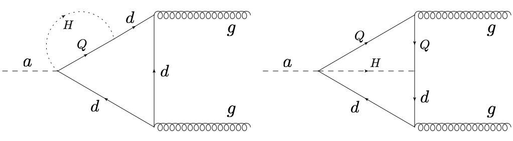
Figure 1: Example of two-loop contributions to axion-gluon couplings of order ${\cal O}\left(\frac{g_{3}^{2}\tilde{Y}_{d}Y_{d}^{\dagger}}{(16\pi^{2})^{2}}\right)$

References

- Peccei and Quinn (1977a) R. D. Peccei and H. R. Quinn, CP Conservation in the Presence of Instantons, Phys. Rev. Lett. 38 (1977a) 1440.
- Peccei and Quinn (1977b) R. D. Peccei and H. R. Quinn, Constraints Imposed by CP Conservation in the Presence of Instantons, Phys. Rev. D 16 (1977b) 1791.
- Weinberg (1978) S. Weinberg, A New Light Boson?, Phys. Rev. Lett. 40 (1978) 223.
- Wilczek (1978) F. Wilczek, Problem of Strong and Invariance in the Presence of Instantons, Phys. Rev. Lett. 40 (1978) 279.
- Kim (1979) J. E. Kim, Weak Interaction Singlet and Strong CP Invariance, Phys. Rev. Lett. 43 (1979) 103.
- Shifman et al. (1980) M. A. Shifman, A. Vainshtein, and V. I. Zakharov, Can Confinement Ensure Natural CP Invariance of Strong Interactions?, Nucl. Phys. B 166 (1980) 493.
- Dine et al. (1981) M. Dine, W. Fischler, and M. Srednicki, A Simple Solution to the Strong CP Problem with a Harmless Axion, Phys. Lett. B 104 (1981) 199.
- Zhitnitsky (1980) A. Zhitnitsky, On Possible Suppression of the Axion Hadron Interactions. (In Russian), Sov. J. Nucl. Phys. 31 (1980) 260.
- Preskill et al. (1983) J. Preskill, M. B. Wise, and F. Wilczek, Cosmology of the Invisible Axion, Phys. Lett. B 120 (1983) 127.
- Abbott and Sikivie (1983) L. F. Abbott and P. Sikivie, A Cosmological Bound on the Invisible Axion, Phys. Lett. B 120 (1983) 133.
- Dine and Fischler (1983) M. Dine and W. Fischler, The Not So Harmless Axion, Phys. Lett. B 120 (1983) 137.
- Di Luzio et al. (2020) L. Di Luzio, M. Giannotti, E. Nardi, and L. Visinelli, The landscape of QCD axion models, Phys. Rept. 870 (2020) 1, arXiv:2003.01100 [hep-ph].
- Hawking (1987) S. W. Hawking, Quantum Coherence Down the Wormhole, Phys. Lett. B 195 (1987) 337.
- Giddings and Strominger (1988) S. B. Giddings and A. Strominger, Loss of Incoherence and Determination of Coupling Constants in Quantum Gravity, Nucl. Phys. B 307 (1988) 854.
- Banks and Seiberg (2011) T. Banks and N. Seiberg, Symmetries and Strings in Field Theory and Gravity, Phys. Rev. D 83 (2011) 084019, arXiv:1011.5120 [hep-th].
- Graham et al. (2015) P. W. Graham, D. E. Kaplan, and S. Rajendran, Cosmological Relaxation of the Electroweak Scale, Phys. Rev. Lett. 115 (2015) 221801, arXiv:1504.07551 [hep-ph].
- Georgi et al. (1986) H. Georgi, D. B. Kaplan, and L. Randall, Manifesting the Invisible Axion at Low-energies, Phys. Lett. B 169 (1986) 73.
- Srednicki (1985) M. Srednicki, Axion Couplings to Matter. 1. CP Conserving Parts, Nucl. Phys. B 260 (1985) 689.
- Izaguirre et al. (2017) E. Izaguirre, T. Lin, and B. Shuve, Searching for Axionlike Particles in Flavor-Changing Neutral Current Processes, Phys. Rev. Lett. 118 (2017) 111802, arXiv:1611.09355 [hep-ph].
- Björkeroth et al. (2018) F. Björkeroth, E. J. Chun, and S. F. King, Flavourful Axion Phenomenology, JHEP 08 (2018) 117, arXiv:1806.00660 [hep-ph].
- Gavela et al. (2019) M. B. Gavela, R. Houtz, P. Quilez, R. Del Rey, and O. Sumensari, Flavor constraints on electroweak ALP couplings, Eur. Phys. J. C 79 (2019) 369, arXiv:1901.02031 [hep-ph].
- Bauer et al. (2020) M. Bauer, M. Neubert, S. Renner, M. Schnubel, and A. Thamm, Axionlike Particles, Lepton-Flavor Violation, and a New Explanation of and , Phys. Rev. Lett. 124 (2020) 211803, arXiv:1908.00008 [hep-ph].
- Albrecht et al. (2020) J. Albrecht, E. Stamou, R. Ziegler, and R. Zwicky, Flavoured axions in the tail of Bq → +- and B → ∗ form factors, JHEP 21 (2020) 139, arXiv:1911.05018 [hep-ph].
- Martin Camalich et al. (2020) J. Martin Camalich, M. Pospelov, P. N. H. Vuong, R. Ziegler, and J. Zupan, Quark Flavor Phenomenology of the QCD Axion, Phys. Rev. D 102 (2020) 015023, arXiv:2002.04623 [hep-ph].
- Endo et al. (2020) M. Endo, S. Iguro, and T. Kitahara, Probing flavor-violating ALP at Belle II, JHEP 06 (2020) 040, arXiv:2002.05948 [hep-ph].
- Ishida et al. (2021) H. Ishida, S. Matsuzaki, and Y. Shigekami, New perspective in searching for axionlike particles from flavor physics, Phys. Rev. D 103 (2021) 095022, arXiv:2006.02725 [hep-ph].
- Calibbi et al. (2021) L. Calibbi, D. Redigolo, R. Ziegler, and J. Zupan, Looking forward to lepton-flavor-violating ALPs, JHEP 09 (2021) 173, arXiv:2006.04795 [hep-ph].
- Carmona et al. (2021) A. Carmona, C. Scherb, and P. Schwaller, Charming ALPs, JHEP 08 (2021) 121, arXiv:2101.07803 [hep-ph].
- Chakraborty et al. (2021) S. Chakraborty, M. Kraus, V. Loladze, T. Okui, and K. Tobioka, Heavy QCD axion in b→s transition: Enhanced limits and projections, Phys. Rev. D 104 (2021) 055036, arXiv:2102.04474 [hep-ph].
- Davoudiasl et al. (2021) H. Davoudiasl, R. Marcarelli, N. Miesch, and E. T. Neil, Searching for flavor-violating ALPs in Higgs boson decays, Phys. Rev. D 104 (2021) 055022, arXiv:2105.05866 [hep-ph].
- Bauer et al. (2021a) M. Bauer, M. Neubert, S. Renner, M. Schnubel, and A. Thamm, Flavor probes of axion-like particles, (2021a), arXiv:2110.10698 [hep-ph].
- Coloma et al. (2022) P. Coloma, P. Hernández, and S. Urrea, New bounds on axion-like particles from MicroBooNE, (2022), arXiv:2202.03447 [hep-ph].
- Gori et al. (2020) S. Gori, G. Perez, and K. Tobioka, KOTO vs. NA62 Dark Scalar Searches, JHEP 08 (2020) 110, arXiv:2005.05170 [hep-ph].
- Mimasu and Sanz (2015) K. Mimasu and V. Sanz, ALPs at Colliders, JHEP 06 (2015) 173, arXiv:1409.4792 [hep-ph].
- Jaeckel and Spannowsky (2016) J. Jaeckel and M. Spannowsky, Probing MeV to 90 GeV axion-like particles with LEP and LHC, Phys. Lett. B 753 (2016) 482, arXiv:1509.00476 [hep-ph].
- Brivio et al. (2017) I. Brivio, M. B. Gavela, L. Merlo, K. Mimasu, J. M. No, R. del Rey, and V. Sanz, ALPs Effective Field Theory and Collider Signatures, Eur. Phys. J. C 77 (2017) 572, arXiv:1701.05379 [hep-ph].
- Bauer et al. (2017a) M. Bauer, M. Neubert, and A. Thamm, LHC as an Axion Factory: Probing an Axion Explanation for with Exotic Higgs Decays, Phys. Rev. Lett. 119 (2017a) 031802, arXiv:1704.08207 [hep-ph].
- Bauer et al. (2017b) M. Bauer, M. Neubert, and A. Thamm, Collider Probes of Axion-Like Particles, JHEP 12 (2017b) 044, arXiv:1708.00443 [hep-ph].
- Alonso-Álvarez et al. (2019) G. Alonso-Álvarez, M. B. Gavela, and P. Quilez, Axion couplings to electroweak gauge bosons, Eur. Phys. J. C 79 (2019) 223, arXiv:1811.05466 [hep-ph].
- Ebadi et al. (2019) J. Ebadi, S. Khatibi, and M. Mohammadi Najafabadi, New probes for axionlike particles at hadron colliders, Phys. Rev. D 100 (2019) 015016, arXiv:1901.03061 [hep-ph].
- Döbrich et al. (2019) B. Döbrich, J. Jaeckel, and T. Spadaro, Light in the beam dump - ALP production from decay photons in proton beam-dumps, JHEP 05 (2019) 213, [Erratum: JHEP 10, 046 (2020)], arXiv:1904.02091 [hep-ph].
- Coelho et al. (2020) R. O. Coelho, V. P. Goncalves, D. E. Martins, and M. S. Rangel, Production of axionlike particles in collisions at the LHC, HE–LHC and FCC: A phenomenological analysis, Phys. Lett. B 806 (2020) 135512, arXiv:2002.06027 [hep-ph].
- Haghighat et al. (2020) G. Haghighat, D. Haji Raissi, and M. Mohammadi Najafabadi, New collider searches for axionlike particles coupling to gluons, Phys. Rev. D 102 (2020) 115010, arXiv:2006.05302 [hep-ph].
- Bonnefoy et al. (2021a) Q. Bonnefoy, L. Di Luzio, C. Grojean, A. Paul, and A. N. Rossia, The anomalous case of axion EFTs and massive chiral gauge fields, JHEP 07 (2021a) 189, arXiv:2011.10025 [hep-ph].
- Flórez et al. (2021) A. Flórez, A. Gurrola, W. Johns, P. Sheldon, E. Sheridan, K. Sinha, and B. Soubasis, Probing axionlike particles with final states from vector boson fusion processes at the LHC, Phys. Rev. D 103 (2021) 095001, arXiv:2101.11119 [hep-ph].
- Wang et al. (2021a) D. Wang, L. Wu, J. M. Yang, and M. Zhang, Photon-jet events as a probe of axionlike particles at the LHC, Phys. Rev. D 104 (2021a) 095016, arXiv:2102.01532 [hep-ph].
- d’Enterria (2021) D. d’Enterria, Collider constraints on axion-like particles, in Workshop on Feebly Interacting Particles (2021) arXiv:2102.08971 [hep-ex].
- Li et al. (2021) S.-Y. Li, Z.-Y. Li, P.-C. Lu, and Z.-G. Si, Precise evaluation of and axion-like particle production, Chin. Phys. C 45 (2021) 093105, arXiv:2103.00409 [hep-ph].
- Goncalves et al. (2021) V. P. Goncalves, D. E. Martins, and M. S. Rangel, Searching for axionlike particles with low masses in pPb and PbPb collisions, Eur. Phys. J. C 81 (2021) 522, arXiv:2103.01862 [hep-ph].
- Alves et al. (2021) A. Alves, A. G. Dias, and D. D. Lopes, Jets and photons spectroscopy of Higgs-ALP interactions, JHEP 10 (2021) 012, arXiv:2105.01095 [hep-ph].
- Bonilla et al. (2022) J. Bonilla, I. Brivio, J. Machado-Rodríguez, and J. F. de Trocóniz, Nonresonant Searches for Axion-Like Particles in Vector Boson Scattering Processes at the LHC, (2022), arXiv:2202.03450 [hep-ph].
- Carmona et al. (2022) A. Carmona, F. Elahi, C. Scherb, and P. Schwaller, The ALPs from the Top: Searching for long lived axion-like particles from exotic top decays, (2022), arXiv:2202.09371 [hep-ph].
- Kling and Quílez (2022) F. Kling and P. Quílez, Axion Searches at the LHC: FASER as a Light Shining through Walls Experiment, (2022), arXiv:2204.03599 [hep-ph].
- Chala et al. (2021) M. Chala, G. Guedes, M. Ramos, and J. Santiago, Running in the ALPs, Eur. Phys. J. C 81 (2021) 181, arXiv:2012.09017 [hep-ph].
- Bonilla et al. (2021) J. Bonilla, I. Brivio, M. B. Gavela, and V. Sanz, One-loop corrections to ALP couplings, JHEP 11 (2021) 168, arXiv:2107.11392 [hep-ph].
- Bauer et al. (2021b) M. Bauer, M. Neubert, S. Renner, M. Schnubel, and A. Thamm, The Low-Energy Effective Theory of Axions and ALPs, JHEP 04 (2021b) 063, arXiv:2012.12272 [hep-ph].
- Jarlskog (1985a) C. Jarlskog, Commutator of the Quark Mass Matrices in the Standard Electroweak Model and a Measure of Maximal CP Violation, Phys. Rev. Lett. 55 (1985a) 1039.
- Jarlskog (1985b) C. Jarlskog, A Basis Independent Formulation of the Connection Between Quark Mass Matrices, CP Violation and Experiment, Z. Phys. C 29 (1985b) 491.
- Bonnefoy et al. (2021b) Q. Bonnefoy, E. Gendy, C. Grojean, and J. T. Ruderman, Beyond Jarlskog: 699 invariants for CP violation in SMEFT, (2021b), arXiv:2112.03889 [hep-ph].
- Davidson and Wali (1982) A. Davidson and K. C. Wali, MINIMAL FLAVOR UNIFICATION VIA MULTIGENERATIONAL PECCEI-QUINN SYMMETRY, Phys. Rev. Lett. 48 (1982) 11.
- Calibbi et al. (2017) L. Calibbi, F. Goertz, D. Redigolo, R. Ziegler, and J. Zupan, Minimal axion model from flavor, Phys. Rev. D 95 (2017) 095009, arXiv:1612.08040 [hep-ph].
- Ema et al. (2017) Y. Ema, K. Hamaguchi, T. Moroi, and K. Nakayama, Flaxion: a minimal extension to solve puzzles in the standard model, JHEP 01 (2017) 096, arXiv:1612.05492 [hep-ph].
- Froggatt and Nielsen (1979) C. D. Froggatt and H. B. Nielsen, Hierarchy of Quark Masses, Cabibbo Angles and CP Violation, Nucl. Phys. B 147 (1979) 277.
- Bonnefoy et al. (2020) Q. Bonnefoy, E. Dudas, and S. Pokorski, Chiral Froggatt-Nielsen models, gauge anomalies and flavourful axions, JHEP 01 (2020) 191, arXiv:1909.05336 [hep-ph].
- Branco et al. (2012) G. C. Branco, P. M. Ferreira, L. Lavoura, M. N. Rebelo, M. Sher, and J. P. Silva, Theory and phenomenology of two-Higgs-doublet models, Phys. Rept. 516 (2012) 1, arXiv:1106.0034 [hep-ph].
- Di Luzio et al. (2021) L. Di Luzio, R. Gröber, and P. Paradisi, Hunting for -violating axionlike particle interactions, Phys. Rev. D 104 (2021) 095027, arXiv:2010.13760 [hep-ph].
- Dekens et al. (2022) W. Dekens, J. de Vries, and S. Shain, CP-violating axion interactions in effective field theory, (2022), arXiv:2203.11230 [hep-ph].
- Coleman et al. (1969) S. R. Coleman, J. Wess, and B. Zumino, Structure of phenomenological Lagrangians. 1., Phys. Rev. 177 (1969) 2239.
- Callan et al. (1969) C. G. Callan, Jr., S. R. Coleman, J. Wess, and B. Zumino, Structure of phenomenological Lagrangians. 2., Phys. Rev. 177 (1969) 2247.
- Feruglio (1993) F. Feruglio, The Chiral approach to the electroweak interactions, Int. J. Mod. Phys. A 8 (1993) 4937, arXiv:hep-ph/9301281.
- Feldmann et al. (2015) T. Feldmann, T. Mannel, and S. Schwertfeger, Renormalization Group Evolution of Flavour Invariants, JHEP 10 (2015) 007, arXiv:1507.00328 [hep-ph].
- Yu and Zhou (2021a) B. Yu and S. Zhou, Sufficient and Necessary Conditions for CP Conservation in the Case of Degenerate Majorana Neutrino Masses, Phys. Rev. D 103 (2021a) 035017, arXiv:2009.12347 [hep-ph].
- Wang et al. (2021b) Y. Wang, B. Yu, and S. Zhou, Flavor invariants and renormalization-group equations in the leptonic sector with massive Majorana neutrinos, JHEP 09 (2021b) 053, arXiv:2107.06274 [hep-ph].
- Jenkins and Manohar (2009) E. E. Jenkins and A. V. Manohar, Algebraic Structure of Lepton and Quark Flavor Invariants and CP Violation, JHEP 10 (2009) 094, arXiv:0907.4763 [hep-ph].
- Trautner (2019) A. Trautner, Systematic construction of basis invariants in the 2HDM, JHEP 05 (2019) 208, arXiv:1812.02614 [hep-ph].
- Yu and Zhou (2021b) B. Yu and S. Zhou, Hilbert Series for Leptonic Flavor Invariants in the Minimal Seesaw Model, (2021b), arXiv:2107.11928 [hep-ph].
- Jenkins et al. (2018a) E. E. Jenkins, A. V. Manohar, and P. Stoffer, Low-Energy Effective Field Theory below the Electroweak Scale: Operators and Matching, JHEP 03 (2018a) 016, arXiv:1709.04486 [hep-ph].
- Jenkins et al. (2018b) E. E. Jenkins, A. V. Manohar, and P. Stoffer, Low-Energy Effective Field Theory below the Electroweak Scale: Anomalous Dimensions, JHEP 01 (2018b) 084, arXiv:1711.05270 [hep-ph].
- Galda et al. (2021) A. M. Galda, M. Neubert, and S. Renner, ALP — SMEFT interference, JHEP 06 (2021) 135, arXiv:2105.01078 [hep-ph].
- Grojean et al. (2013) C. Grojean, E. E. Jenkins, A. V. Manohar, and M. Trott, Renormalization Group Scaling of Higgs Operators and \Gamma(h - \gamma \gamma), JHEP 04 (2013) 016, arXiv:1301.2588 [hep-ph].
- Jenkins et al. (2013) E. E. Jenkins, A. V. Manohar, and M. Trott, Renormalization Group Evolution of the Standard Model Dimension Six Operators I: Formalism and lambda Dependence, JHEP 10 (2013) 087, arXiv:1308.2627 [hep-ph].
- Jenkins et al. (2014) E. E. Jenkins, A. V. Manohar, and M. Trott, Renormalization Group Evolution of the Standard Model Dimension Six Operators II: Yukawa Dependence, JHEP 01 (2014) 035, arXiv:1310.4838 [hep-ph].
- Alonso et al. (2014) R. Alonso, E. E. Jenkins, A. V. Manohar, and M. Trott, Renormalization Group Evolution of the Standard Model Dimension Six Operators III: Gauge Coupling Dependence and Phenomenology, JHEP 04 (2014) 159, arXiv:1312.2014 [hep-ph].
- Yu and Zhou (2022) B. Yu and S. Zhou, CP violation and flavor invariants in the seesaw effective field theory, (2022), arXiv:2203.10121 [hep-ph].
- Bilal (2008) A. Bilal, Lectures on Anomalies, (2008), arXiv:0802.0634 [hep-th].