Post-Newtonian expansion of the spin-precession invariant for eccentric-orbit non-spinning extreme-mass-ratio inspirals to 9PN and $e^{16}$

Abstract

We calculate the eccentricity dependence of the high-order post-Newtonian (PN) expansion of the spin-precession invariant $\psi$ for eccentric-orbit extreme-mass-ratio inspirals with a Schwarzschild primary. The series is calculated in first-order black hole perturbation theory through direct analytic expansion of solutions in the Regge-Wheeler-Zerilli formalism, using a code written in Mathematica. Modes with small values of $l$ are found via the Mano-Suzuki-Takasugi (MST) analytic function expansion formalism for solutions to the Regge-Wheeler equation. Large-$l$ solutions are found by applying a PN expansion ansatz to the Regge-Wheeler equation. Previous work has given $\psi$ to 9.5PN order and to order $e^{2}$ (i.e., the near circular orbit limit). We calculate the expansion to 9PN but to $e^{16}$ in eccentricity. It proves possible to find a few terms that have closed-form expressions, all of which are associated with logarithmic terms in the PN expansion. We also compare the numerical evaluation of our PN expansion to prior numerical calculations of $\psi$ in close orbits to assess its radius of convergence. We find that the series is not as rapidly convergent as the one for the redshift invariant at $r\simeq 10M$ but still yielding $\sim 1\%$ accuracy for eccentricities $e\lesssim 0.25$.

I Introduction

In a set of recent papers, we have presented high post-Newtonian (PN) order analytic expansions of black hole perturbation theory (BHPT) and gravitational self-force quantities at first order in the mass ratio $\varepsilon\ll 1$ for extreme-mass-ratio inspiral (EMRI) binaries in bound eccentric motion about a Schwarzschild black hole. In each case, these results are double expansions in PN order and in powers of the eccentricity $e$. This work included study in the dissipative sector of gravitational wave energy and angular momentum fluxes radiated to infinity Munna (2020); Munna and Evans (2019); Munna et al. (2020); Munna and Evans (2020) and fluxes radiated into the horizon Munna and Evans (2022) and study in the conservative sector of the redshift invariant Munna and Evans (2022). The method involves using the Regge-Wheeler-Zerilli (RWZ) formalism Regge and Wheeler (1957); Zerilli (1970) and making analytic function expansions using the Mano-Suzuki-Takasugi (MST) formalism Mano et al. (1996) and a general-$l$ ansatz to find expansions of the mode functions. The metric perturbations and self-force are derived in the Regge-Wheeler (RW) gauge and mode-sum regularization is used. A sampling of other applications that have used this procedure include Bini and Damour (2013, 2014, 2014a, 2014b); Kavanagh et al. (2015); Forseth et al. (2016); Hopper et al. (2016).

This paper applies those techniques to another gauge-invariant quantity, the spin-precession invariant. This invariant, $\psi$, quantifies the geodetic precession of a gyroscope attached to the smaller mass as it is parallel transported during its orbital motion. The test-body limit of the geodetic precession is well known. We are concerned with the first order in $\varepsilon$ correction to $\psi$, $\Delta\psi$, induced by the small but finite mass of the secondary. For an eccentric orbit, $\psi$ is defined as the fractional precessional angular advance $\Psi$, per azimuthal angular advance $\Phi$, accumulated over one radial libration. The calculation of $\Delta\psi$ bears some similarities to that of the redshift invariant, as they both depend on the metric perturbation at the point mass location. As discussed in Munna and Evans (2022); Hopper et al. (2016), the PN order of individual modes of the local metric perturbation do not increase with $l$, which means that the mode functions and metric perturbation must be calculated for arbitrarily high $l$. This general-$l$ complication is handled by utilizing a PN-expansion ansatz solution to the RW equation valid for all $l$ above the target PN order Bini and Damour (2013, 2014, 2014a); Kavanagh et al. (2015); Hopper et al. (2016); Munna and Evans (2022).

Calculating $\Delta\psi$ presents new challenges. One is the need to calculate the (conservative) self-force itself. (In contrast, the redshift invariant only required the metric perturbation.) Calculation of all of the metric perturbation components and the components of the self-force is roughly an order of magnitude more computationally costly than the effort involved in finding the redshift invariant. Furthermore, the self-force is gauge dependent. Fortunately, the regularization is performed on the $l$-modes of the spin-precession invariant itself, extracting the gauge invariant result directly. However, the mode-sum regularization procedure in this case requires two regularization parameters in order for the mode-sum to converge.

The spin-precession invariant was originally calculated for circular orbits in Dolan et al. (2014), both numerically and as a full arbitrary-mass-ratio PN expansion to 3PN absolute order. (Note that in contrast to previous papers on fluxes, where we referred to relative PN orders, here we connote PN order with the power of the PN compactness parameter ($y$ or $1/p$) appearing in the expansion of $\Delta\psi$, as is conventional in papers on the spin invariant.) The spin-precession invariant was previously found Kavanagh et al. (2015) to 21.5PN in the circular-orbit limit using BHPT analytic expansions. In the eccentric-orbit case, results were found both numerically and as a 3PN expansion in Akcay et al. (2017). Note, that the circular-orbit quantity $\Delta\psi^{\rm circ}$ is not the same as its eccentric-orbit counterpart $\Delta\psi^{\rm ecc}$ when the latter is taken in the limit $e\rightarrow 0$. The eccentric-orbit definition relies on angular changes accumulated over one radial libration. In the limit as $e\rightarrow 0$, apsidal advance becomes indistinguishable from azimuthal advance but the difference in these definitions involves the order $\varepsilon$ correction to the apsidal advance. The calculation of the eccentric-orbit version was separately found Akcay et al. (2017) to 9.5PN. The $\mathcal{O}(e^{2})$ correction was then computed to 3PN in Akcay et al. (2017), to 6PN in Kavanagh et al. (2017), to 9PN in Bini et al. (2018), and then to 9.5PN in Bini and Geralico (2019). The present work finds $\Delta\psi$ to 9PN but takes the eccentricity expansion to $e^{16}$, breaking away from the nearly circular orbit limit.

Conservative quantities like the spin-precession invariant supply crucial terms in effective-one-body (EOB) potentials Barack et al. (2010); Le Tiec et al. (2012); Bini and Damour (2014b); Bini et al. (2016); Hopper et al. (2016); Kavanagh et al. (2017); Bini et al. (2018, 2019, 2020a, 2020b)) and also contribute directly to the EMRI cumulative phase at post-1 adiabatic order Hinderer and Flanagan (2008). A procedure is described by Kavanagh et al. (2017) for translating the expansion of $\Delta\psi$ to the EOB gyrogravitomagnetic potential $g_{S*}(1/r,p_{r},p_{\varphi})$, thus informing the spin-orbit sector of EOB dynamics. The spin-precession invariant expansion in this paper can be transcribed to EOB form to enhance further the knowledge of the spin-orbit part.

The structure of this paper is as follows: In Sec. II we briefly outline (i) the setup of the orbital motion problem, (ii) the MST formalism for computing solutions and PN expansions of specific $l$ modes, (iii) the procedure for finding general-$l$ parts of the expansion, and (iv) the calculation of the (local) metric perturbation. Sec. III (i) defines the spin-precession invariant, (ii) describes the background tetrad and how to calculate the precession, (iii) summarizes how the first-order correction to the spin precession is computed with a definition that is gauge invariant, and (iv) how mode-sum regularization is applied to the spin invariant. Then, the results of our calculations are presented in Sec. IV, first as a PN expansion in the compactness parameter $1/p$ and second as an expansion in the PN parameter $y$. Our expansions are also evaluated numerically at a pair of close orbital separations and compared to prior numerical calculations. Sec. V concludes with summary and outlook.

Throughout this paper we choose units such that $c=G=1$, though $\eta=1/c$ is briefly reintroduced for PN-expansion bookkeeping purposes. We use metric signature $(-+++)$. Our notation for the RWZ formalism follows that found in Forseth et al. (2016); Munna et al. (2020), which in part derives from notational changes for tensor spherical harmonics and perturbation amplitudes made by Martel and Poisson Martel and Poisson (2005). For the MST formalism, we largely make use of the discussion and notation found in the review by Sasaki and Tagoshi Sasaki and Tagoshi (2003).

II Formalism for black hole perturbations and post-Newtonian expansions

A pair of recent papers Munna (2020); Munna and Evans (2022) outlined our approach to calculating the first-order metric perturbation for eccentric-orbit non-spinning EMRIs and PN expanding regularized quantities. The more recent paper used the technique to derive the high-order PN expansion of the redshift invariant. For our present purpose, in calculating the spin-precession invariant, and to set the notation, we briefly recite in this section the calculational approach. See Munna (2020); Munna and Evans (2022) for further details.

II.1 Bound orbits and PN compactness parameters

The secondary is treated as a point mass $\mu$ in bound geodesic orbit about a Schwarzschild black hole of mass $M$, with $\varepsilon=\mu/M\ll 1$. We use Schwarzschild coordinates $x^{\mu}=(t,r,\theta,\varphi)$ that produce the line element

$$ds^{2}=-fdt^{2}+f^{-1}dr^{2}+r^{2}\left(d\theta^{2}+\sin^{2}\theta\,d\varphi^{2}\right),$$ (1)

with $f=1-2M/r$. Restricting the motion to the equatorial plane, the four-velocity is

$$u^{\alpha}(\tau)=\frac{dx_{p}^{\alpha}(\tau)}{d\tau}=\left(\frac{{\mathcal{E}}}{f_{p}},u^{r},0,\frac{{\mathcal{L}}}{r_{p}^{2}}\right),$$ (2)

where $\mathcal{E}$ and $\mathcal{L}$, the specific energy and angular momentum, are constants of the motion and the subscript $p$ indicates evaluation along the worldline of the particle. The orbital motion is reparameterized using Darwin’s parameters $(\chi,p,e)$ Darwin (1959); Cutler et al. (1994); Barack and Sago (2010), connected by

$${\mathcal{E}}^{2} =\frac{(p-2)^{2}-4e^{2}}{p(p-3-e^{2})},\quad{\mathcal{L}}^{2}=\frac{p^{2}M^{2}}{p-3-e^{2}},$$

$$\qquad\quad r_{p}\left(\chi\right)=\frac{pM}{1+e\cos\chi}.$$ (3)

Here $p$ is the semilatus rectum and its reciprocal $1/p$ serves as one choice for a PN compactness parameter. In the Darwin parameterization, one radial libration corresponds to $2\pi$ advance in $\chi$. Motion in the other three coordinates, along with proper time $\tau$, are found by integrating ordinary differential equations (ODEs) in $\chi$ Cutler et al. (1994); Hopper et al. (2015). Most of these equations of motion can be initially PN expanded and then integrated analytically order by order. For example, the radial period is found from the following integral

$$T_{r}=\int_{0}^{2\pi}\frac{r_{p}\left(\chi\right)^{2}}{M(p-2-2e\cos\chi)}\left[\frac{(p-2)^{2}-4e^{2}}{p-6-2e\cos\chi}\right]^{1/2}d\chi,$$

and it is immediately clear how the integrand may be expanded in powers of $1/p$, resulting in a series of elementary trigonometric integrals. From that expansion then follows an expansion for the radial frequency, $\Omega_{r}=2\pi/T_{r}$. In the case of azimuthal motion, the solution for $\varphi_{p}(\chi)$ can be obtained analytically prior to PN expansion

$$\Omega_{\varphi}=\frac{4}{T_{r}}\left(\frac{p}{p-6-2e}\right)^{1/2}\,K\left(-\frac{4e}{p-6-2e}\right),$$ (4)

where $K(m)$ is the complete elliptic integral of the first kind Gradshteyn et al. (2007). The solution can be readily PN expanded in $1/p$. Once the mean angular rate is known, the alternative standard PN compactness parameter $y=(M\Omega_{\varphi})^{2/3}$ can be obtained in terms of $1/p$, and then inverted for $p(y)$. For eccentric motion, PN expansion in $1/p$ or $y$ leads to related expansion in powers of eccentricity $e$.

II.2 Gravitational perturbations and analytic expansion of $l$-mode solutions

On a Schwarzschild background, we can obtain metric perturbations either via the Regge-Wheeler-Zerilli (RWZ) Regge and Wheeler (1957); Zerilli (1970) formalism (see recent uses Hopper and Evans (2010); Hopper et al. (2016); Munna and Evans (2022)) or by use of the Bardeen-Press-Teukolsky equation and radiation gauge Kavanagh et al. (2017). In this paper, we adhere to our previous RWZ approach, in which the RWZ master equations have the following form in the frequency domain (FD)

$$\left[\frac{d^{2}}{dr_{*}^{2}}+\omega^{2}-V_{l}(r)\right]X_{lmn}(r)=Z_{lmn}(r).$$ (5)

Here $r_{*}=r+2M\ln|r/2M-1|$ is the tortoise coordinate, $\omega\equiv\omega_{mn}=m\Omega_{\varphi}+n\Omega_{r}$ are discrete frequencies from the multiperiodic background geodesic motion, and the FD source term is

$$Z_{lmn} =\frac{1}{T_{r}}\int_{0}^{2\pi}(G_{lm}(t)\,\delta[r-r_{p}(t)]$$

$$\qquad\qquad\qquad+F_{lm}(t)\,\delta^{\prime}[r-r_{p}(t)])e^{i\omega t}dt.$$ (6)

The source terms and potentials $V_{l}(r)$ are ($l+m$) parity-dependent. The source terms can be found in Hopper and Evans (2010).

The homogeneous version of the master equation yields two independent (causal) solutions. One, $X_{lmn}^{\rm in}=X_{lmn}^{-}$, is a downgoing wave at the future horizon, while the other, $X_{lmn}^{\rm up}=X_{lmn}^{+}$, is an outgoing wave at future null infinity. The odd-parity homogeneous (Regge-Wheeler) equation is more readily solved. For even parity cases of $l+m$, the Regge-Wheeler equation can be solved again and those solutions can be transformed to their even-parity counterparts using the the Detweiler-Chandrasekhar transformation Chandrasekhar (1975); Chandrasekhar and Detweiler (1975); Chandrasekhar (1983); Berndston (2007).

Once the homogeneous solutions are calculated (discussed below), the inhomogeneous solutions to (5) are found, which starts by computing the normalization coefficients

$$C_{lmn}^{\pm}=\frac{1}{W_{lmn}T_{r}}\int_{0}^{2\pi}\left(\frac{dt}{d\chi}\right)\bigg{[}\frac{1}{f_{p}}G_{lm}(\chi)X^{\mp}_{lmn}+\left(\frac{2M}{r_{p}^{2}f_{p}^{2}}X^{\mp}_{lmn}-\frac{1}{f_{p}}\frac{dX^{\mp}_{lmn}}{dr}\right)F_{lm}(\chi)\bigg{]}e^{i\omega t(\chi)}d\chi,$$ (7)

where $W_{lmn}$ is the Wronskian. The full time-domain solutions follow from applying the method of extended homogeneous solutions Barack et al. (2008), using the combinations $C_{lmn}^{+}X_{lmn}^{+}$ and $C_{lmn}^{-}X_{lmn}^{-}$ (see also Hopper and Evans (2010); Munna (2020)).

As discussed in Munna (2020); Munna and Evans (2022), solutions for the modes of the master function (at least for small values of $l$) are determined using the MST formalism Mano et al. (1996), with an expansion in analytic functions. The odd-parity MST solution for $X_{lmn}^{+}$ (up to arbitrary normalization) is

$$X^{+}_{lmn} =e^{iz}z^{\nu+1}\left(1-\frac{\epsilon}{z}\right)^{-i\epsilon}\sum_{j=-\infty}^{\infty}a_{j}(-2iz)^{j}\frac{\Gamma(j+\nu+1-i\epsilon)\Gamma(j+\nu-1-i\epsilon)}{\Gamma(j+\nu+3+i\epsilon)\Gamma(j+\nu+1+i\epsilon)}\times$$

$$\hskip 270.00041ptU(j+\nu+1-i\epsilon,2j+2\nu+2,-2iz).$$ (8)

Here, $\nu$ is the renormalized angular momentum, defined to make the double-sided summation converge, and $U$ is the irregular confluent hypergeometric function. Other quantities are $\epsilon=2M\omega\eta^{3}$, $z=r\omega\eta$, with $\eta=1/c$ being a reintroduced PN parameter. To obtain a solution, $\nu$ and $a_{j}$ are ascertained through a continued fraction calculation Mano et al. (1996); Sasaki and Tagoshi (2003), which in our application also then leads to series in $\epsilon$ for both. PN expansions of the other terms in (II.2) then follow, with the result expressible in series in both $z$ and $\epsilon$.

The downgoing (or in) solutions $X_{lmn}^{-}$ have similar function expansion

$$X^{-}_{lmn} =e^{-iz}\left(\frac{z}{\epsilon}-1\right)^{-i\epsilon}\left(\frac{\epsilon}{z}\right)^{i\epsilon+1}\sum_{j=-\infty}^{\infty}a_{j}\frac{\Gamma(j+\nu-1-i\epsilon)\Gamma(-j-\nu-2-i\epsilon)}{\Gamma(1-2i\epsilon)}\times$$

$$\hskip 200.0003pt{}_{2}F_{1}(j+\nu-1-i\epsilon,-j-\nu-2-i\epsilon;1-2i\epsilon;1-z/\epsilon),$$ (9)

with $\nu$ and $a_{j}$ here being identical to those in (II.2) (up to overall normalization of the latter). The process of expanding these homogeneous solutions by collecting on powers of $\eta$ is fully described in Munna (2020), based on the methods presented in Kavanagh et al. (2015). As described in Munna and Evans (2022); Kavanagh et al. (2015), $z$-independent factors are removed from these solutions to reduce their complexity, since such factors eventually cancel through appearance in the Wronskian.

As discussed in Bini and Damour (2013); Kavanagh et al. (2015); Munna (2020); Munna and Evans (2022), in conservative sector calculations mode-sum regularization requires summing perturbations over all $l$. This necessitates an alternative approach of directly PN-expanding the homogeneous version of the master equation (5) for general $l$. As shown in Bini and Damour (2013); Kavanagh et al. (2015), the PN-expansion ansatz for solving the RW equation is

$$X_{lmn}^{+} =(z)^{-\nu}(1+A_{2}\eta^{2}+A_{4}\eta^{4}+\cdots+A_{2l}\eta^{2l}+\mathcal{O}(\eta^{2l+1})),$$

$$X_{lmn}^{-} =\left(\frac{\epsilon}{z}\right)^{-\nu-1}(1+B_{2}\eta^{2}+B_{4}\eta^{4}+\cdots+B_{2l}\eta^{2l}+\mathcal{O}(\eta^{2l+1})),$$ (10)

where the $A_{i}$ and $B_{i}$ are functions of $z,\epsilon,l$. The ansatz breaks down at PN orders at and above $\mathcal{O}(\eta^{2l})$. If a target PN order $P$ is set, the ansatz will be useless for $l\leq P$. For those finite number of modes, the MST formalism is used instead. Once $\nu$ is found by PN-expanding the continued fraction calculation, the homogeneous RW equation becomes

$$\left[\left(1-\frac{\epsilon}{z}\right)\frac{\partial}{\partial z}\left(\left(1-\frac{\epsilon}{z}\right)\frac{\partial}{\partial z}\right)+\eta^{2}+\left(1-\frac{\epsilon}{z}\right)\left(\frac{l(l+1)}{z^{2}}-\frac{3\epsilon}{z^{3}}\right)\eta^{2}\right]X^{\pm}_{lmn}=0.$$ (11)

The ODE is then solved order by order. Even-parity homogeneous solutions are again found using the Detweiler-Chandrasekhar transformation.

As previously noted Munna and Evans (2022), the expansion of the even-parity normalization integral is the bottleneck in the calculation, requiring for example $\sim$7 days and 20GB of memory on the UNC supercomputing cluster Longleaf to reach 10PN and $e^{20}$ relative order. Furthermore, two relative PN orders and three orders in $e$ are lost in constructing and regularizing the spin-precession invariant. Thus, our expansion is restricted to 9PN (8PN relative order) and $e^{16}$.

II.3 Metric perturbation $l$-modes and non-radiative modes

Since we use RWZ gauge, calculation of the $l$-modes of the metric perturbation (locally) follows the procedure discussed in Section II of Munna and Evans (2022) (see also earlier work Hopper et al. (2016); Hopper and Evans (2010)). Briefly, the metric components as functions of $\chi$ are

$$p_{rr}^{l}(\chi) =\left(\frac{d\chi}{dr}\right)\sum_{mn}\frac{Y_{lm}(\pi/2,0)}{f}C^{\pm}_{lmn}e^{im\varphi-i\omega t}\Bigg{\{}\left[\left(\frac{dr}{d\chi}\right)\frac{\Lambda(\lambda+1)}{fr}-\left(\frac{dr}{d\chi}\right)\frac{\Lambda}{f}A(\chi)+r\left(\frac{dA(\chi)}{d\chi}\right)\right]X^{\pm}_{lmn}(\chi)$$

$$+(rA(\chi)-\Lambda)\left(\frac{dX^{\pm}_{lmn}(\chi)}{d\chi}\right)+r\frac{d}{d\chi}\left[f\left(\frac{d\chi}{dr}\right)\left(\frac{dX^{\pm}_{lmn}(\chi)}{d\chi}\right)\right]\Bigg{\}},$$

$$p_{tr}^{l}(\chi) =\sum_{mn}Y_{lm}(\pi/2,0)C^{\pm}_{lmn}e^{im\varphi-i\omega t}(-i\omega)\left[r\left(\frac{d\chi}{dr}\right)\left(\frac{dX^{\pm}_{lmn}(\chi)}{d\chi}\right)+rB(\chi)X^{\pm}_{lmn}(\chi)\right],$$

$$p_{tt}^{l}(\chi) =f^{2}p_{rr}^{l,\pm},$$

$$p_{AB}^{l}(\chi) =r^{2}\Omega_{AB}\sum_{mn}Y_{lm}(\pi/2,0)C^{\pm}_{lmn}e^{im\varphi-i\omega t}\left[f\left(\frac{d\chi}{dr}\right)\partial_{\chi}X_{lmn}^{e,\pm}+A(\chi)X_{lmn}^{e,\pm}\right],$$

$$p_{tB}^{l}(\chi) =\left(\frac{f}{2}\right)\sum_{mn}X^{lm}_{B}(\pi/2,0)C^{\pm}_{lmn}e^{im\varphi-i\omega t}\left(\frac{d\chi}{dr}\right)\frac{d}{d\chi}(rX^{\pm}_{lmn}),$$

$$p_{rB}^{l}(\chi) =\left(\frac{r}{2f}\right)\sum_{mn}X^{lm}_{B}(\pi/2,0)C^{\pm}_{lmn}e^{im\varphi-i\omega t}(-i\omega)X^{\pm}_{lmn},$$ (12)

with

$$\lambda =\frac{1}{2}(l+2)(l-1),\qquad\qquad\Lambda=\lambda+\frac{3M}{r},$$

$$A(r) =\frac{1}{r\Lambda}\left[\lambda(\lambda+1)+\frac{3M}{r}\left(\lambda+\frac{2M}{r}\right)\right],$$

$$B(r) =\frac{1}{rf\Lambda}\left[\lambda\left(1-\frac{3M}{r}\right)-\frac{3M^{2}}{r^{2}}\right].$$ (13)

The up ($+$) or in ($-$) mode functions are used depending upon which side in $r$ of the point mass the evaluation is taken. The perturbation $l$-modes (once sums over $m$ are made) are continuous, but $C^{0}$, at the particle location. Sums over $m$ involve application of the addition theorem for spherical harmonics. In Munna and Evans (2022) we discuss the most efficient way of calculating PN expansions of the resulting sums over $m$ (see Section IID of that paper). The spin-precession invariant is calculated from the local self-force, which involves the metric perturbation and its derivatives. Expressions for the derivatives can be easily derived from (II.3). The $l$-modes of the metric perturbation derivatives are discontinuous across the particle location, a fact that is important in the regularization of the spin-precession invariant.

Another aspect of computing the self-force is that, in applying a derivative with respect to $\chi$, an expansion over powers of eccentricity will lose an order in $e$. Moreover, the eccentricity expansions lose a total of 3 orders in $e$ in moving from the self-force to the spin invariant. The computation of high-order series in $e$ is the most consuming part of the construction of the metric perturbations, particularly initially in the case of general $l$. However, added investigation showed that this difficulty can be avoided in the latter case by observing that the general-$l$ metric perturbations yield finite polynomials in $e$ on an individual PN-order basis. These polynomials increase in degree linearly with PN order. Once this pattern was recognized, PN terms in the general-$l$ expansion could be determined in closed form with only a low-order (imbedded) polynomial in eccentricity. The computational bottleneck was then transferred to the specific-$l$ part of the calculation, which does not simplify in the same fashion. The resulting change in the technique allowed the spin-precession invariant to be computed to much higher order in eccentricity at lower PN orders. For example, it allowed us to determine the 4PN function $\Delta\psi_{4}$ to $e^{30}$.

Finally, to complete the metric perturbation and self-force calculation, the radiative modes must be augmented to include the nonradiative $l=0$ and $l=1$ modes, originally found by Zerilli Zerilli (1970) but gauge transformed Sago et al. (2008) to maintain asymptotic flatness. We listed those modes in our previous paper Munna and Evans (2022), and they are described more fully in Hopper et al. (2016) and in earlier papers cited therein.

III Procedure for calculating the spin-precession invariant

III.1 Overview

The smaller body is assumed to be endowed with a spin $s_{\alpha}$, which undergoes precession during the orbital motion about the heavier mass. The spin is parallel transported $Ds_{\alpha}/d\tau=0$ along the geodesic with its tangent vector $u^{\alpha}$, and the spin maintains its orthogonality $s_{\alpha}u^{\alpha}=0$ and the constancy of its norm $s_{\alpha}s^{\alpha}$. This spin-orbit, or geodetic, precession has a nonzero rate of advance in the test-body limit ($\mu=0$) and a self-force correction at first order in the mass ratio $\varepsilon$ and beyond. We seek to calculate the first-order correction to the precession in bound eccentric orbits about a nonspinning (Schwarzschild) primary (thus eliminating consideration of Lense-Thirring precession). Our presentation follows that of Dolan et al. (2014); Akcay et al. (2017); Kavanagh et al. (2017), which we summarize in this section.

The spin-precession invariant for eccentric orbits is a generalization given by Akcay et al. (2017) of the definition used for circular orbits Dolan et al. (2014). An invariant $\psi$ is defined via a ratio that involves the accumulated azimuthal phase $\Phi$ and the accumulated precession of the spin vector $\Psi$ over one radial libration period $T_{r}$. Explicitly, the quantity is given by

$$\psi=1-\frac{\Psi}{\Phi}.$$ (14)

This scalar is a function of the mass ratio $\varepsilon$ (i.e., subject to self-force correction $\Delta\psi$) and orbital parameters. The latter are best chosen as the observable frequencies $\Omega_{r}$ and $\Omega_{\varphi}$, lending the definition of $\psi$ a gauge invariant character. This procedure is directly analogous to that in constructing the redshift invariant Munna and Evans (2022), where the frequencies were held fixed through first order in the mass ratio. Since $\Phi=\Omega_{\varphi}T_{r}$ will itself be fixed, only the self-force correction $\Delta\Psi$ need be computed.

The invariant $\psi$ encodes a portion of the first-order conservative dynamics, giving it relevance to the creation of waveform templates for LISA. How $\psi$ can be transcribed to the EOB gyrogravitomagnetic ratio quantity $g_{S*}(1/r,p_{r},p_{\varphi})$, which partially characterizes the spin-orbit sector of the EOB Hamiltonian, was mapped out in Kavanagh et al. (2017). The expansion of $\psi$ helps describe the case where the smaller body is (weakly) spinning.

III.2 Spin precession and background reference frame

The behavior of $\Psi$ is found by computing the parallel transport of $s_{\alpha}$ along a geodesic of the perturbed (regularized) metric. To facilitate the calculation, a reference frame tetrad $e^{\alpha}_{a}$ is introduced (here $\alpha$ is the spacetime index and $a$ indicates the frame element). Then, the spin components in the frame precess Akcay et al. (2017) according to

$$\frac{d\textbf{s}}{d\tau} =\textbf{w}\times\textbf{s},$$

$$(\textbf{s})_{i} =e^{\alpha}_{i}s_{\alpha},$$

$$(\textbf{w})_{i} =-\frac{1}{2}\epsilon_{ijk}w^{jk},$$

$$w_{ij} =-g_{\alpha\beta}e_{i}^{\alpha}\frac{De_{j}^{\beta}}{d\tau}.$$ (15)

The precessional angular velocity components use the base symbol $w$ instead of $\omega$ to avoid confusion with the discrete frequency spectrum $\omega_{mn}$ of the gravitational perturbations. The angular velocity is subject to the choice made for the reference frame.

A suitable frame in the background ($\mu\rightarrow 0$ limit) was given by Marck Marck (1983) (see also Akcay et al. (2017); Kavanagh et al. (2017), as well as Cheng and Evans (2013) for a different application), aligned with one leg perpendicular to the orbital (equatorial) plane and another directed along the line with the primary

$$e_{0}^{\mu} =u^{\mu}=\left(\frac{\mathcal{E}}{f},u^{r},0,\frac{\mathcal{L}}{r^{2}}\right),$$

$$e_{1}^{\mu} =\frac{1}{f\sqrt{1+\mathcal{L}^{2}/r^{2}}}(u^{r},f\mathcal{E},0,0),$$

$$e_{2}^{\mu} =(0,0,1/r,0),$$

$$e_{3}^{\mu} =\frac{1}{r\sqrt{1+\mathcal{L}^{2}/r^{2}}}\left(\frac{\mathcal{E}\mathcal{L}}{f},\mathcal{L}u^{r},0,1+\frac{\mathcal{L}^{2}}{r^{2}}\right).$$ (16)

This polar alignment can be maintained when $\mu\neq 0$. The frame is non-inertial and a gyroscope will appear to precess with frequency $\dot{\Psi}=w_{13}$. (The precession can also be found by making a $U(1)$ transformation Cheng and Evans (2013) in the equatorial plane to an inertial frame.) At lowest order the (background) geodetic angular rate is

$$w^{(0)}_{13}=\frac{\mathcal{E}\mathcal{L}}{r^{2}+\mathcal{L}^{2}}.$$ (17)

III.3 Spin precession and self-force in the perturbed frame

The accumulated phase of the spin precession is then

$$\Psi=\oint w_{13}(\tau)d\tau=\Psi_{0}+\Delta\Psi,$$ (18)

with the integral taken over one period of radial motion. The last part of the expression splits $\Psi$ into 0th and 1st order components, with $\Delta\Psi$ being the first-order (conservative) correction we seek. Here, $\Delta\Psi$ refers to the perturbation measured when the orbital frequencies have been held constant.

The procedure to compute $\Delta\Psi$ is established in Akcay et al. (2017); Kavanagh et al. (2017); Bini et al. (2018). Assuming that $\delta\Psi$ is a correction calculated without holding the orbital frequencies fixed, $\Delta\Psi$ is recovered by subtracting off perturbations in the frequencies

$$\Delta\Psi=\delta\Psi-\frac{\partial\Psi_{0}}{\partial\Omega_{r}}\delta\Omega_{r}-\frac{\partial\Psi_{0}}{\partial\Omega_{\varphi}}\delta\Omega_{\varphi}.$$ (19)

An alternative calculation uses first-order changes in $T_{r}$ and $\Phi$ Akcay et al. (2017)

$$\Delta\Psi=\delta\Psi-\frac{\partial\Psi_{0}}{\partial T_{r}}\delta T_{r}-\frac{\partial\Psi_{0}}{\partial\Phi}\delta\Phi,$$ (20)

which we found more computationally convenient. Note that henceforth, except for our use of $\Psi_{0}$ and $w^{(0)}_{13}$, lowest-order quantities will simply be denoted by their plain base symbol, while most first-order corrections will explicitly carry a $\delta$ (perturbed frequencies) or $\Delta$ (fixed frequencies) prefix. The exception is the metric perturbation $p_{\mu\nu}$, where the notation already indicates a first-order quantity.

At first order, the integral for $\Psi$ experiences a change due to corrections in both $w_{13}$ and $\tau$. The result is Barack and Sago (2011); Akcay et al. (2017)

$$\delta\Psi=\int_{0}^{2\pi}\left(\frac{\delta w_{13}}{w_{13}}-\frac{\delta u^{r}}{u^{r}}\right)w_{13}\,\frac{d\tau}{d\chi}\,d\chi.$$ (21)

The correction to $w_{13}$ can be found Akcay et al. (2017); Kavanagh et al. (2017) via expansion of its definition

$$\delta w_{13}=\frac{1}{2}w_{13}\,p_{\mu\nu}e_{0}^{\mu}e_{0}^{\nu} +\delta\Gamma_{[31]0}$$ (22)

$$+(c_{01}e_{1}^{\mu}+c_{03}e_{3}^{\mu})\,\,e_{\nu[3}\nabla_{\mu}e^{\nu}_{1]}.$$

In deriving the expression above, a total derivative ($d/d\tau$) term has been neglected. The first term is proportional to the $p_{00}$ tetrad projection of the metric perturbation (not $p_{tt}$) and the second term is the tetrad projection of the correction to the affine connection

$$\delta\Gamma_{[31]0}=(\delta\Gamma_{\mu\nu\beta}-p_{\mu\lambda}\Gamma^{\lambda}_{\nu\beta})e^{\mu}_{[3}e^{\nu}_{1]}u^{\beta}.$$ (23)

The third term involves coefficients $c_{01}$ and $c_{03}$ that come from the variation of the tetrad

$$c_{01} =\frac{1}{f\sqrt{1+\mathcal{L}^{2}/r^{2}}}(\mathcal{E}\delta u^{r}_{BS}-u^{r}\delta\mathcal{E}_{BS}),$$ (24)

$$c_{03} =\frac{\delta\mathcal{L}_{BS}}{r\sqrt{1+\mathcal{L}^{2}/r^{2}}}.$$ (25)

Within these latter coefficients are terms, $\delta\mathcal{E}_{BS}$ and $\delta\mathcal{L}_{BS}$, that are $\chi$-dependent conservative corrections to the (specific) energy and angular momentum defined by Barack and Sago Barack and Sago (2011)

$$\delta\mathcal{E}_{BS}(\chi) =\delta\mathcal{E}_{BS}(0)-\int_{0}^{\chi}F_{t}^{\rm cons}\frac{d\tau}{d\chi^{\prime}}\,d\chi^{\prime},$$ (26)

$$\delta\mathcal{L}_{BS}(\chi) =\delta\mathcal{L}_{BS}(0)+\int_{0}^{\chi}F_{\varphi}^{\rm cons}\frac{d\tau}{d\chi^{\prime}}\,d\chi^{\prime}.$$ (27)

The first term (integration constant) in each of these equations is the shift that occurs at periastron. These are explicitly shown Barack and Sago (2011) to be

$$\delta\mathcal{E}_{BS}(0) =\frac{(1+e)^{2}(p-2-2e)}{4e(p-3-e^{2})}\left[\frac{(1-e)^{2}(p-2+2e)}{Mp^{3/2}\sqrt{(p-2)^{2}-4e^{2}}}\int_{0}^{\pi}F_{\varphi}^{\rm cons}\frac{d\tau}{d\chi}d\chi+\int_{0}^{\pi}F_{t}^{\rm cons}\frac{d\tau}{d\chi}d\chi\right],$$ (28)

$$\delta\mathcal{L}_{BS}(0) =\frac{Mp^{3/2}\sqrt{(p-2)^{2}-4e^{2}}}{4e(p-3-e^{2})}\left[\frac{(1-e)^{2}(p-2+2e)}{Mp^{3/2}\sqrt{(p-2)^{2}-4e^{2}}}\int_{0}^{\pi}F_{\varphi}^{\rm cons}\frac{d\tau}{d\chi}d\chi+\int_{0}^{\pi}F_{t}^{\rm cons}\frac{d\tau}{d\chi}d\chi\right].$$ (29)

Lastly, $\delta u^{r}_{BS}$ is the first-order correction to the radial velocity. It can be derived from the normalization of the four-velocity condition (in the background spacetime Barack and Sago (2011)), which leads to $\mathcal{E}\delta\mathcal{E}_{BS}-u^{r}\delta u^{r}_{BS}-r^{-2}f\mathcal{L}\delta\mathcal{L}_{BS}=0$ and from there to

$$\delta u^{r}_{BS}=\frac{\mathcal{E}}{u^{r}}\delta\mathcal{E}_{BS}-\frac{f}{r^{2}u^{r}}\mathcal{L}\delta\mathcal{L}_{BS}.$$ (30)

As usual, the conservative part of the self-force, $F_{\mu}^{\rm cons}$, is given Barack and Sago (2011) by the symmetric combination

$$F_{\mu}^{\rm cons}=\frac{1}{2}\left(F_{\mu}(\chi)+\epsilon^{(\mu)}F_{\mu}(-\chi)\right),$$ (31)

where $\epsilon^{(\mu)}=(-1,1,1,-1)$. Using the retarded self-force in the expression above yields a singular result at the particle location. Instead, the regularized self-force can be found using the regular metric perturbation $p^{R}_{\mu\nu}$ in

$$F^{\alpha}_{R}=\frac{1}{2}(g^{\alpha\delta}u^{\beta}-2g^{\alpha\beta}u^{\delta}-u^{\alpha}u^{\beta}u^{\delta})u^{\gamma}\nabla_{\delta}p^{R}_{\beta\gamma}.$$ (32)

However, since we are concerned with computing a single scalar invariant, it is simpler to work instead with the full, unregularized self-force, decomposed into $l$-modes. This leads to an $l$-mode decomposition of the (unregularized) spin invariant correction, with modes $\Delta\psi^{l}$. We then apply mode-sum regularization directly to the spin-precession invariant.

Hence, with the $l$-modes of the retarded metric perturbation and self-force available, it is straightforward to evaluate $\mathcal{E}_{BS}^{l}$, $\mathcal{L}_{BS}^{l}$, and $\Gamma_{[31]0}^{l}$. The rest of the calculation for $\delta\Psi^{l}$ is then condensed Bini et al. (2018) to the following integral

$$\delta\Psi^{l}=\int_{0}^{2\pi}\left[\delta\Gamma_{[31]0}^{l}+\left(\frac{(r^{2}+\mathcal{L}^{2})(3M-r)\mathcal{L}}{r^{5}(u^{r})^{2}}-\frac{\mathcal{L}}{r^{2}}\right)\delta\mathcal{E}_{BS}^{l}+\left(\frac{\mathcal{E}}{r^{2}}-\frac{\mathcal{E}\mathcal{L}^{2}(3M-r)}{r^{5}(u^{r})^{2}}\right)\delta\mathcal{L}_{BS}^{l}\right]\frac{d\tau}{d\chi}d\chi.$$ (33)

Then, $\Delta\Psi^{l}$ can be determined from $\delta\Psi^{l}$ by removal of the frequency corrections, which involves use of the following formulas Akcay et al. (2017); Bini et al. (2018)

$$\delta T_{r}^{l} =\int_{0}^{2\pi}\left(\frac{\delta\mathcal{E}_{BS}^{l}}{\mathcal{E}}-\frac{\delta(u^{r}_{BS})^{l}}{u^{r}}\right)\frac{\mathcal{E}}{f}\frac{d\tau}{d\chi}d\chi,$$ (34)

$$\delta\Phi^{l} =\int_{0}^{2\pi}\left(\frac{\delta\mathcal{L}_{BS}^{l}}{\mathcal{L}}-\frac{\delta(u^{r}_{BS})^{l}}{u^{r}}\right)\frac{\mathcal{L}}{r^{2}}\frac{d\tau}{d\chi}d\chi.$$ (35)

III.4 PN and eccentricity expansion issues

Even though we have not belabored the process, each step in this procedure involves calculating an analytic PN expansion using Mathematica. (Illustrative short expansions of various intermediate quantities in the procedure can be found in Section III of Kavanagh et al. (2017).) Given eccentric orbital motion, the PN expansion necessarily involves an expansion in powers of eccentricity $e$ as well. We have sought to go as deeply as possible in PN order and (especially) eccentricity order. High-order expansion in eccentricity opens up the possibility of finding eccentricity-dependent terms that have closed-form expressions or infinite series with analytically-known coefficient sequences Munna and Evans (2019, 2020, 2022).

We restate for emphasis one issue with calculating the PN and eccentricity expansions of the spin-precession invariant. As we have discussed, the procedure begins with calculating the mode functions $X^{\pm}_{lmn}$ and their normalizations $C_{lmn}^{\pm}$. Assume that $C_{lmn}^{+}$, for example, has been calculated in the general-$l$ case to a relative PN order of $\mathcal{P}$ and to order $e^{2\mathcal{N}}$ in eccentricity. We find that once derivatives have been taken, to calculate the metric perturbation and the self-force, and the various projections have been made, the expansion of the spin-precession invariant has lost two relative orders in $\mathcal{P}$ and two orders in $e^{2}$ (i.e., two order in $\mathcal{N}$). For example, if $C_{lmn}^{+}$ were known in the general-$l$ case to 8PN (relative) and $e^{20}$, the computation of the general-$l$ contribution to the spin invariant is limited to 6PN relative order (7PN absolute order, as it is conventionally defined) and $e^{16}$. One caveat, however, is that the general-$l$ expansion does not contribute to the spin precession at half-integer orders. Thus, as long as the specific-$l$ contributions are appropriately extended, the final result in this example would be an expansion for $\psi$ that reaches 7.5PN (absolute) and $e^{16}$.

III.5 Regularization

The final step in the procedure is regularization. As mentioned in Sec. III.3, instead of regularizing the self-force itself, we calculate $l$-modes of the spin invariant using $l$-modes of the unregularized retarded self-force. Then, we make a mode-sum regularization of the spin invariant itself, in a procedure that is similar to but slightly more involved than the way in which we previously regularized the redshift invariant Munna and Evans (2022). Because the spin invariant involves derivatives of the metric perturbation, $l$-mode contributions to the singular behavior grow like $l$. Mode-sum regularization requires subtracting off terms from the expansion of the singular field

$$\Delta\psi=\sum_{l=0}^{\infty}\left(\Delta\psi^{l,\pm}_{\rm ret}\mp A_{S}(2l+1)-B_{S}\right).$$ (36)

The calculation on the right is direction dependent, based on whether the particle location is approached from outside or inside of $r_{p}$, but yields the same final value. The coefficients, $A_{S}$ and $B_{S}$, are the two regularization parameters required to allow the sum to converge. However, usually regularization parameters are defined by decomposing every vector and tensor component into a sum over scalar spherical harmonics. Then, each regularization parameter is $l$ independent. In the present application, our $l$ is different and refers to the tensor spherical harmonic index, with the implication Wardell and Warburton (2015) that $A_{S}$ at least is not completely independent of $l$ but changes value for $l=0$ and $l=1$. Furthermore, neither $A_{S}$ nor $B_{S}$ are known a priori.

The workaround for the latter issue involves using the general-$l$ expansion. Because $A_{S}$ and $B_{S}$ must match the large-$l$ behavior of $\Delta\psi^{l,\rm ret}$, we can expand our general-$l$ result for $\Delta\psi^{l}_{\rm ret}$ about $l=\infty$ to find two coefficients, $A_{\infty}$ and $B_{\infty}$. Then theoretically, $B_{\infty}=B_{S}$ (for all $l$) and $A_{\infty}=A_{S}$ for $l\geq 2$. The qualification is that regularization and decomposition of the singular field is usually discussed in the context of Lorenz gauge Detweiler and Whiting (2003). While we are working in a different gauge, mode-sum regularization carries across Barack and Ori (2001) to select other gauges, with RWZ gauge Thompson et al. (2019) being one.

The remaining problem is the behavior of $A_{S}$ when $l=0,1$. The solution is to recognize that $A_{S}$ flips sign across the location of the point mass Wardell and Warburton (2015) (see (II.3)), allowing (36) to be replaced by Kavanagh et al. (2017); Bini et al. (2018)

$$\Delta\psi=\sum_{l=0}^{\infty}\left(\frac{1}{2}(\Delta\psi^{l,+}_{\rm ret}+\Delta\psi^{l,-}_{\rm ret})-B_{\infty}\right).$$ (37)

However, there is no reason to use (37) for every $l$. We can instead use (36) for all $l\geq 2$ and reserve use of (37) for only the $l=0$ and $l=1$ modes. The net effect is to reduce the calculation by roughly 50%.

IV PN Expansions of the Spin-Precession Invariant

The procedure in the previous two sections was utilized to compute the spin-precession invariant expansion to 9PN order and to $e^{16}$ in eccentricity. We present the expansions in this section using both $1/p$ and $y$ as compactness parameters. The expansions are given in this paper to 8PN order, with the full series being available in electronic form at the Black Hole Perturbation Toolkit BHP website and at our research group website UNC .

IV.1 Spin-precession invariant as an expansion in $1/p$

Previous work in the circular-orbit limit has revealed Akcay et al. (2017) the general PN structure of $\Delta\psi$ to 9.5PN order. Expressed in terms of the compactness parameter $1/p$, the form of the expansion is

$$\Delta\psi= \,\,\frac{\Delta\psi_{1}^{p}}{p}+\frac{\Delta\psi_{2}^{p}}{p^{2}}+\frac{\Delta\psi_{3}^{p}}{p^{3}}+\left(\Delta\psi_{4}^{p}+\Delta\psi_{4L}^{p}\log p\right)\frac{1}{p^{4}}+\left(\Delta\psi_{5}^{p}+\Delta\psi_{5L}^{p}\log p\right)\frac{1}{p^{5}}+\frac{\Delta\psi_{11/2}^{p}}{p^{11/2}}$$

$$+\left(\Delta\psi_{6}^{p}+\Delta\psi_{6L}^{p}\log p\right)\frac{1}{p^{6}}+\frac{\Delta\psi_{13/2}^{p}}{p^{13/2}}+(\Delta\psi_{7}^{p}+\Delta\psi_{7L}^{p}\log p+\Delta\psi_{7L2}^{p}\log^{2}p)\frac{1}{p^{7}}+\frac{\Delta\psi_{15/2}^{p}}{p^{15/2}}$$

$$+\left(\Delta\psi_{8}^{p}+\Delta\psi_{8L}^{p}\log p+\Delta\psi_{8L2}^{p}\log^{2}p\right)\frac{1}{p^{8}}+\left(\Delta\psi_{17/2}^{p}+\Delta\psi_{17/2L}^{p}\log p\right)\frac{1}{p^{17/2}}$$

$$+\left(\Delta\psi_{9}^{p}+\Delta\psi_{9L}^{p}\log p+\Delta\psi_{9L2}^{p}\log^{2}p\right)\frac{1}{p^{9}}+\cdots.$$ (38)

Because this is a first-order self-force result, the entire right hand side should be viewed as multiplied by a factor of $\mu/M$. For eccentric orbits, each of the quantities $\Delta\psi^{p}_{k}$, for different $k$, is no longer just a number but rather a function of the eccentricity $e$. The purpose of this section is to show the form of these functions.

In discussing energy and angular momentum fluxes (see e.g., Munna et al. (2020)) it is conventional to factor out the circular-orbit limit with $p^{-5}$ and refer to terms in the expansion by their relative PN order. Thus, the Peters-Mathews flux is 0PN relative. In the spin-precession invariant expansion, the leading-order term is $p^{-1}$ and we will refer to this as the 1PN (absolute) term. In our nomenclature, a $k$PN term is one that is proportional to $p^{-k}$.

The first three functions were all found previously Akcay et al. (2017) and shown to have closed forms

$$\Delta\psi_{1}^{p}= -1,$$ (39)

$$\Delta\psi_{2}^{p}= \frac{9+4e^{2}}{4},$$ (40)

$$\Delta\psi_{3}^{p}= \left(\frac{739}{16}-\frac{123\pi^{2}}{64}\right)+e^{2}\left(\frac{341}{16}-\frac{123\pi^{2}}{256}\right)-\frac{e^{4}}{2}.$$ (41)

Beyond 3PN order, only the circular-orbit behavior Akcay et al. (2017) and first term, $e^{2}$, in eccentricity were known previously. The $e^{2}$ terms through 6PN had been calculated by Kavanagh et al. (2017) and Bini et al. (2018) had found the $e^{2}$ behavior through 9PN. Our present work extends every term through 9PN order to $e^{16}$ in eccentricity, allowing key parts of the functions $\Delta\psi^{p}_{k}(e)$ to be isolated in many cases and allowing us to find in a few cases complete, closed-form expressions.

The 4PN term is a case in which having enough terms in the eccentricity expansion allows us to identify elemental parts of the eccentricity functions. The behavior of the 4PN spin-precession invariant is reminiscent of the 3PN energy flux. We find first that the 4PN log term has a closed-form expression. Then, that same function reappears in the 4PN non-log term. It is then possible to see a grouping, as a series, that contains all of the log-transcendental numbers (which we denote by $\Delta\psi^{p,\chi}_{4}$ in analogy to similar functions in the energy flux, angular momentum flux, and redshift invariant expansions). We display $\Delta\psi^{p,\chi}_{4}$ in this paper to $e^{16}$. The remaining part of the 4PN non-log term is a polynomial on the appearance of $\pi^{2}$ and a remaining rational-number series. That latter rational-number series is also displayed here to $e^{16}$. The breakdown of the 4PN term is as follows:

$$\Delta\psi_{4}^{p}= \bigg{(}-\frac{587831}{2880}-\frac{37961e^{2}}{160}-\frac{28129e^{4}}{480}-\frac{19015e^{6}}{1152}-\frac{138247e^{8}}{15360}-\frac{12431e^{10}}{2048}$$

$$-\frac{327985e^{12}}{73728}-\frac{56393e^{14}}{16384}-\frac{725137e^{16}}{262144}+\cdots\bigg{)}+\pi^{2}\bigg{(}\frac{31697}{6144}-\frac{23729e^{2}}{4096}-\frac{23761e^{4}}{16384}\bigg{)}$$

$$-2\left[\gamma_{E}+\log\left(\frac{8(1-e^{2})^{3/2}}{1+\sqrt{1-e^{2}}}\right)\right]\Delta\psi_{4L}^{p}+\Delta\psi_{4}^{p,\chi},$$ (42)

$$\Delta\psi_{4}^{p,\chi}= \left(-\frac{2216\log(2)}{15}+\frac{729\log(3)}{5}\right)+\left(\frac{55384\log(2)}{15}-\frac{10206\log(3)}{5}\right)e^{2}+\bigg{(}-\frac{205917\log(2)}{5}+$$

$$\frac{3620943\log(3)}{320}+\frac{1953125\log(5)}{192}\bigg{)}e^{4}+\left(\frac{11518508\log(2)}{45}+\frac{3995649\log(3)}{320}-\frac{68359375\log(5)}{576}\right)e^{6}$$

$$+\left(-\frac{1597223897\log(2)}{1350}-\frac{199689627159\log(3)}{409600}+\frac{274244140625\log(5)}{442368}+\frac{678223072849\log(7)}{3686400}\right)e^{8}$$

$$+\left(\frac{27567693977\log(2)}{4500}+\frac{1474172887599\log(3)}{512000}-\frac{71310546875\log(5)}{36864}-\frac{678223072849\log(7)}{307200}\right)e^{10}$$

$$+\bigg{(}-\frac{39584616236117\log(2)}{1134000}-\frac{2523359744732097\log(3)}{458752000}+\frac{1806540009765625\log(5)}{445906944}$$

$$+\frac{77643655602826369\log(7)}{6370099200}\bigg{)}e^{12}+\bigg{(}\frac{7796904819020377\log(2)}{47628000}-\frac{96876093468033783\log(3)}{3211264000}$$

$$-\frac{173056322265625\log(5)}{3121348608}-\frac{1313351173426101691\log(7)}{31850496000}\bigg{)}e^{14}+\bigg{(}-\frac{1349495913968063023\log(2)}{2286144000}$$

$$+\frac{44537688184006902231\log(3)}{164416716800}-\frac{131695624109951171875\log(5)}{1826434842624}$$

$$+\frac{9397785802951526436547\log(7)}{97844723712000}+\frac{81402749386839761113321\log(11)}{4794391461888000}\bigg{)}e^{16}+\cdots,$$ (43)

$$\Delta\psi_{4L}^{p}= -\left(\frac{628}{15}+\frac{268e^{2}}{5}+\frac{37e^{4}}{10}\right).$$ (44)

Our result for the 4PN term is exceptional in one regard. As mentioned in Sec. II.3, we are able to exploit a feature in the eccentricity expansion of the general-$l$ part of the metric perturbation. At any given PN order, the eccentricity expansion of the general-$l$ modes truncates at some power, which depends upon metric component and PN order but not $l$. The only contributions to higher powers of $e$ beyond this truncation point come from the (MST-derived) specific-$l$ calculation. We used this feature to calculate the 4PN term to much higher order in eccentricity ($e^{30}\,$!). The resulting eccentricity series gave us another opportunity to look for additional closed-form expressions and infinite series with analytically recognizable coefficient sequences. While no additional such functions were identified, we are providing the full 4PN term to $e^{30}$ in the online repositories BHP ; UNC .

The breakdown of the 5PN term is similar. Once again, we have enough information in the lengthy eccentricity expansion to see that the 5PN log term is a polynomial. The 5PN log term reappears in the 5PN non-log term. There is then a $\chi$-like grouping of terms that can be isolated in the 5PN non-log function. There is a closed-form expression identifiable that multiplies $\pi^{2}$ and the remainder is a rational-number series.

$$\Delta\psi_{5}^{p}= \bigg{(}-\frac{48221551}{19200}-\frac{948244847e^{2}}{403200}+\frac{213024509e^{4}}{134400}+\frac{6416801e^{6}}{19200}+\frac{21598637e^{8}}{161280}+\frac{61987887e^{10}}{716800}$$

$$+\frac{2519343e^{12}}{40960}+\frac{482228861e^{14}}{10321920}+\frac{25511929e^{16}}{688128}+\cdots\bigg{)}+\pi^{2}\bigg{(}\frac{2483157}{8192}+\frac{21274445e^{2}}{49152}$$ (45)

$$-\frac{1392915e^{4}}{65536}-\frac{322801e^{6}}{65536}-\frac{123}{256}\left(1-e^{2}\right)^{5/2}\bigg{)}-2\left[\gamma_{E}+\log\left(\frac{8(1-e^{2})^{3/2}}{1+\sqrt{1-e^{2}}}\right)\right]\Delta\psi_{5L}^{p}+\Delta\psi_{5}^{p,\chi},$$

$$\Delta\psi_{5}^{p,\chi}= \bigg{(}\frac{155894\log(2)}{105}-\frac{31347\log(3)}{28}\bigg{)}+\bigg{(}-\frac{4518706\log(2)}{105}+\frac{4430133\log(3)}{320}+\frac{9765625\log(5)}{1344}\bigg{)}e^{2}$$

$$+\bigg{(}\frac{103760293\log(2)}{180}-\frac{31627665\log(3)}{1792}-\frac{3850703125\log(5)}{16128}\bigg{)}e^{4}+\bigg{(}-\frac{7257966409\log(2)}{1512}-$$

$$\frac{412866263889\log(3)}{286720}+\frac{185751484375\log(5)}{73728}+\frac{96889010407\log(7)}{221184}\bigg{)}e^{6}+\bigg{(}\frac{1363049747783\log(2)}{37800}$$

$$+\frac{193316307253281\log(3)}{11468800}-\frac{179678368984375\log(5)}{12386304}-\frac{458460436354739\log(7)}{44236800}\bigg{)}e^{8}$$

$$+\bigg{(}-\frac{12831673840577\log(2)}{45360}-\frac{7224124751440749\log(3)}{91750400}+\frac{8043417607578125\log(5)}{148635648}+$$

$$\frac{355523097835854137\log(7)}{3538944000}\bigg{)}e^{10}+\bigg{(}\frac{183330830280580517\log(2)}{95256000}-\frac{805502573948046501\log(3)}{12845056000}$$

$$-\frac{422974129832265625\log(5)}{4161798144}-\frac{14424400165163864701\log(7)}{25480396800}\bigg{)}e^{12}$$

$$+\bigg{(}-\frac{4506759544919422111\log(2)}{444528000}+\frac{4528120073662511265537\log(3)}{1438646272000}$$

$$-\frac{12939671783145268046875\log(5)}{22373826822144}+\frac{17394718021348645585769\log(7)}{8153726976000}$$

$$+\frac{81402749386839761113321\log(11)}{559345670553600}\bigg{)}e^{14}+\bigg{(}\frac{8175474265144902875339\log(2)}{192036096000}$$

$$-\frac{487753344707796027586053\log(3)}{23018340352000}+\frac{8271291205691128966015625\log(5)}{1073943687462912}$$ (46)

$$-\frac{6796075855660208932297721\log(7)}{1174136684544000}-\frac{1236467363350808533619347277\log(11)}{402728882798592000}\bigg{)}e^{16}+\cdots,$$

$$\Delta\psi_{5L}^{p}= \,\,\left(\frac{11153}{35}+\frac{11341e^{2}}{15}+\frac{46467e^{4}}{280}-\frac{1119e^{6}}{560}\right).$$ (47)

Like the redshift invariant, the first half-integer function appears at 5.5PN order. We find it to be a rational-number infinite series, multiplied by an overall factor of $\pi$

$$\Delta\psi_{11/2}^{p}= \,\,\pi\bigg{(}\frac{49969}{315}+\frac{319609e^{2}}{630}+\frac{21280909e^{4}}{100800}+\frac{2619467e^{6}}{362880}-\frac{5582939e^{8}}{580608000}+\frac{19566341e^{10}}{5806080000}$$

$$-\frac{1283076269e^{12}}{2601123840000}-\frac{3498178499e^{14}}{21849440256000}+\frac{4868320009201e^{16}}{251705551749120000}+\cdots\bigg{)}.$$ (48)

At 6PN order we found a structure similar to 4PN and 5PN, but with some added complexity. Once again, we were able to find a closed-form expression for the (6PN) log term, though it is not simply a polynomial. The 6PN log term reappears in the 6PN non-log function. We group the log-transcendental number terms into a $\chi$-like series again. Then, an added wrinkle is the appearance of a $\pi^{4}$ term (which is a polynomial in $e$) as well as a more complicated closed-form expression multiplying $\pi^{2}$. The remainder is, again, a rational-number series. This breakdown is given by

$$\Delta\psi_{6}^{p}= \,\,\bigg{(}-\frac{1900873914203}{101606400}-\frac{465224579689e^{2}}{5080320}-\frac{2021344615177e^{4}}{33868800}-\frac{481812394033e^{6}}{203212800}$$

$$+\frac{908657975293e^{8}}{1625702400}+\frac{115787009753e^{10}}{464486400}+\frac{63855468847e^{12}}{371589120}+\frac{663864852377e^{14}}{5202247680}$$

$$+\frac{237445545371e^{16}}{2378170368}+\cdots\bigg{)}+\pi^{4}\bigg{(}-\frac{7335303}{131072}-\frac{146026515e^{2}}{1048576}-\frac{17998485e^{4}}{524288}+\frac{679545e^{6}}{16777216}\bigg{)}$$

$$+\pi^{2}\bigg{[}\frac{7254777827}{2359296}+\frac{32034966215e^{2}}{2359296}+\frac{77315025809e^{4}}{9437184}+\frac{5875228633e^{6}}{12582912}-\frac{326041715e^{8}}{33554432}$$

$$+\left(-\frac{21405}{2048}-\frac{26549e^{2}}{8192}\right)\left(1-e^{2}\right)^{5/2}\bigg{]}-2\left[\gamma_{E}+\log\left(\frac{8(1-e^{2})^{3/2}}{1+\sqrt{1-e^{2}}}\right)\right]\Delta\psi_{6L}^{p}+\Delta\psi_{6}^{p,\chi},$$ (49)

$$\Delta\psi_{6}^{p,\chi}= \,\,\bigg{[}\bigg{(}-\frac{5637649\log(2)}{630}+\frac{234009\log(3)}{70}+\frac{9765625\log(5)}{9072}\bigg{)}+\bigg{(}\frac{278347639\log(2)}{945}-\frac{159335343\log(3)}{8960}$$

$$-\frac{17193359375\log(5)}{145152}\bigg{)}e^{2}+\bigg{(}-\frac{67298137969\log(2)}{15120}-\frac{6160676211\log(3)}{4480}+\frac{2073211184375\log(5)}{870912}$$

$$+\frac{96889010407\log(7)}{248832}\bigg{)}e^{4}+\bigg{(}\frac{45349640544529\log(2)}{816480}+\frac{31165257813381\log(3)}{1146880}$$

$$-\frac{182206079940625\log(5)}{7962624}-\frac{387081765684929\log(7)}{23887872}\bigg{)}e^{6}+\bigg{(}-\frac{558659555193209\log(2)}{816480}$$

$$-\frac{53870960843541\log(3)}{262144}+\frac{61171359261321875\log(5)}{445906944}+\frac{294158696797354949\log(7)}{1194393600}\bigg{)}e^{8}$$

$$+\bigg{(}\frac{847397764060731841\log(2)}{122472000}+\frac{32809717319486013\log(3)}{1835008000}-\frac{2422221742760078125\log(5)}{5350883328}$$

$$-\frac{2408276754022760847373\log(7)}{1146617856000}\bigg{)}e^{10}+\bigg{(}-\frac{16872974428064804681\log(2)}{321489000}$$

$$+\frac{702548354497142812293\log(3)}{51380224000}-\frac{10596237215626599434375\log(5)}{5393690394624}$$

$$+\frac{16313635952096120303239\log(7)}{1375941427200}+\frac{81402749386839761113321\log(11)}{134842259865600}\bigg{)}e^{12}$$

$$+\bigg{(}\frac{44527790291197983392407\log(2)}{144027072000}-\frac{796933093810646955107709\log(3)}{5754585088000}$$

$$+\frac{110679665407920978635528125\log(5)}{2416373296791552}-\frac{42403949775722831599753919\log(7)}{880602513408000}$$

$$-\frac{151763386707026658481899113\log(11)}{8629904631398400}\bigg{)}e^{14}+\bigg{(}-\frac{1066795518870736337912533\log(2)}{691329945600}$$

$$+\frac{561883567881441059477453079\log(3)}{736586891264000}-\frac{68528286383578337812136246875\log(5)}{173978877368991744}$$

$$+\frac{18715907817618872220720781253\log(7)}{126806761930752000}+\frac{624926196399309721148911875383\log(11)}{2718419958890496000}$$

$$+\frac{91733330193268616658399616009\log(13)}{8698943868449587200}\bigg{)}e^{16}+\cdots\bigg{]},$$ (50)

$$\Delta\psi_{6L}^{p}= \,\,\frac{454397}{3780}+\frac{2384929e^{2}}{1890}+\frac{45143023e^{4}}{30240}+\frac{5037481e^{6}}{20160}-\frac{2387e^{8}}{960}-\left(\frac{146}{5}+\frac{37e^{2}}{5}\right)\left(1-e^{2}\right)^{5/2}.$$ (51)

The 6.5PN term is similar in form to the 5.5PN term, a rational-number infinite series with an overall factor of $\pi$

$$\Delta\psi_{13/2}^{p}= \,\,\pi\bigg{(}-\frac{2620819}{2100}-\frac{1586616631e^{2}}{235200}-\frac{5337465431e^{4}}{940800}-\frac{273779628487e^{6}}{406425600}$$

$$+\frac{23921441479e^{8}}{5419008000}-\frac{2200323829e^{10}}{19267584000}+\frac{6113757813097e^{12}}{655483207680000}$$

$$+\frac{200661326003101e^{14}}{48942746173440000}-\frac{13890607636693243e^{16}}{7047755448975360000}+\cdots\bigg{)}.$$ (52)

At 7PN order, there are additional complexities. Here, a $\log^{2}p$ term makes its first appearance and we find the closed-form expression for that term. The 7PN log term then inherits the general structure of the 4PN non-log term. It features a reappearance of the 7PN $\log^{2}p$ term, a $\chi$-like series grouping, and a remaining rational-number series. The 7PN non-log term is the first appearance of a much more complicated expansion, which features numerous transcendental number terms. While we have calculated it to $e^{16}$, it is sufficiently complicated that we only present the first few coefficients here. The entire term is available online BHP ; UNC . The breakdown of the 7PN terms is

$$\Delta\psi_{7}^{p}= \,\,\bigg{(}-\frac{1282190594044678657}{7041323520000}+\frac{1316474014843\gamma_{E}}{43659000}-\frac{3396608\gamma_{E}^{2}}{1575}+\frac{25657561505749\pi^{2}}{2477260800}$$

$$+\frac{341587582057\pi^{4}}{1006632960}+\frac{2783260080883\log(2)}{43659000}-\frac{5149696\gamma_{E}\log(2)}{1575}-\frac{931328\log^{2}(2)}{1575}$$

$$+\frac{282123979047\log(3)}{8624000}-\frac{936036}{175}\gamma_{E}\log(3)-\frac{936036}{175}\log(2)\log(3)-\frac{468018\log^{2}(3)}{175}+\frac{63488\zeta(3)}{15}$$

$$-\frac{361328125\log(5)}{24192}\bigg{)}+\bigg{(}-\frac{2888955324477314921}{2347107840000}+\frac{1075057978433\gamma_{E}}{4851000}-\frac{7219504\gamma_{E}^{2}}{525}$$

$$+\frac{465082867177871\pi^{2}}{6606028800}+\frac{314165501411\pi^{4}}{335544320}+\frac{2387982140729\log(2)}{8731800}-\frac{79652512}{315}\gamma_{E}\log(2)$$

$$-\frac{80263696\log^{2}(2)}{175}-\frac{299782486660473\log(3)}{275968000}+\frac{15912612}{175}\gamma_{E}\log(3)+\frac{15912612}{175}\log(2)\log(3)$$

$$+\frac{7956306\log^{2}(3)}{175}+\frac{2411543359375\log(5)}{2838528}+\frac{678223072849\log(7)}{6082560}+\frac{134944\zeta(3)}{5}\bigg{)}e^{2}$$

$$+\bigg{(}-\frac{113070994466917771}{58677696000}+\frac{1472132397523\gamma_{E}}{4656960}-\frac{1627684\gamma_{E}^{2}}{105}+\frac{1927756649323\pi^{2}}{18350080}$$

$$-\frac{230109551791\pi^{4}}{268435456}+\frac{4388818385774297\log(2)}{349272000}+\frac{1697626904}{525}\gamma_{E}\log(2)+\frac{3404199436\log^{2}(2)}{525}$$

$$+\frac{157855832267967\log(3)}{7168000}-\frac{262324089}{400}\gamma_{E}\log(3)-\frac{262324089}{400}\log(2)\log(3)-\frac{262324089\log^{2}(3)}{800}$$

$$-\frac{7905614284523125\log(5)}{1072963584}-\frac{1044921875\gamma_{E}\log(5)}{1008}-\frac{1044921875\log(2)\log(5)}{1008}$$

$$-\frac{1044921875\log^{2}(5)}{2016}-\frac{1107664826873969\log(7)}{109486080}+30424\zeta(3)\bigg{)}e^{4}+\cdots,$$ (53)

$$\Delta\psi_{7L}^{p}= \,\,\bigg{(}-\frac{1316474014843}{87318000}-\frac{1048904096833e^{2}}{9702000}-\frac{6494255602463e^{4}}{46569600}-\frac{2123271392639e^{6}}{55883520}$$

$$-\frac{1333068673e^{8}}{352800}-\frac{148643207731e^{10}}{88704000}-\frac{5888596871e^{12}}{5376000}-\frac{204908923e^{14}}{258048}$$

$$-\frac{63078518299e^{16}}{103219200}+\cdots\bigg{)}-4\left[\gamma_{E}+\log\left(\frac{8(1-e^{2})^{3/2}}{1+\sqrt{1-e^{2}}}\right)\right]\Delta\psi_{7L2}^{p}+\Delta\psi_{7L}^{p,\chi},$$ (54)

$$\Delta\psi_{7L}^{p,\chi}= \,\,\bigg{(}-\frac{602624\log(2)}{225}+\frac{468018\log(3)}{175}\bigg{)}+\bigg{(}\frac{155814256\log(2)}{1575}-\frac{7956306\log(3)}{175}\bigg{)}e^{2}$$

$$+\bigg{(}-\frac{865090292\log(2)}{525}+\frac{262324089\log(3)}{800}+\frac{1044921875\log(5)}{2016}\bigg{)}e^{4}+\bigg{(}\frac{7561620022\log(2)}{525}$$

$$+\frac{418174083\log(3)}{200}-\frac{11494140625\log(5)}{1512}\bigg{)}e^{6}+\bigg{(}-\frac{27112112493049\log(2)}{283500}$$

$$-\frac{339134405423319\log(3)}{7168000}+\frac{238205615234375\log(5)}{4644864}+\frac{507989081563901\log(7)}{27648000}\bigg{)}e^{8}$$

$$+\bigg{(}\frac{2438441188502\log(2)}{3375}+\frac{2457755729168913\log(3)}{7168000}-\frac{328215185546875\log(5)}{1548288}-$$

$$\frac{507989081563901\log(7)}{1843200}\bigg{)}e^{10}+\bigg{(}-\frac{27531157668664681\log(2)}{4961250}-\frac{6481474893571248729\log(3)}{8028160000}$$

$$+\frac{2822922907568359375\log(5)}{4682022912}+\frac{92389498231271366573\log(7)}{47775744000}\bigg{)}e^{12}+$$

$$\bigg{(}\frac{20936989659899360021\log(2)}{625117500}-\frac{171956257323847250841\log(3)}{28098560000}-\frac{510786718173828125\log(5)}{16387080192}$$

$$-\frac{1009210224594126146977\log(7)}{119439360000}\bigg{)}e^{14}+\bigg{(}-\frac{4619194353324708185237\log(2)}{30005640000}$$

$$+\frac{982128291923792960826417\log(3)}{14386462720000}-\frac{2383328610155127138671875\log(5)}{134242960932864}$$ (55)

$$+\frac{18946304992805061334986887\log(7)}{733835427840000}+\frac{1053921396311414387134166987\log(11)}{251705551749120000}\bigg{)}e^{16}+\cdots,$$

$$\Delta\psi_{7L2}^{p}= \,\,-\frac{849152}{1575}-\frac{1804876e^{2}}{525}-\frac{406921e^{4}}{105}-\frac{543667e^{6}}{630}-\frac{10593e^{8}}{560}.$$ (56)

The 7.5PN term is a rational-number infinite series (multiplied by an overall factor of $\pi$), like the two half-integer contributions before it

$$\Delta\psi_{15/2}^{p}= \,\,\pi\bigg{(}\frac{2782895449}{2910600}+\frac{2404331748779e^{2}}{279417600}+\frac{76598649855971e^{4}}{6035420160}+\frac{8047650291899e^{6}}{5267275776}$$

$$-\frac{5292862534207931e^{8}}{10534551552000}-\frac{279109475326162289e^{10}}{27811216097280000}-\frac{4713058120092455293e^{12}}{2336142152171520000}$$

$$-\frac{959696950970026746929e^{14}}{523295842086420480000}-\frac{25409776245923969873e^{16}}{37378274434744320000}+\cdots\bigg{)}.$$ (57)

The description of the breakdown in the 8PN eccentricity functions is essentially the same as what we said about the 7PN terms just prior to (IV.1). We still find a polynomial for the 8PN $\log^{2}p$ term, albeit one order in $e^{2}$ longer. Because of the complexity of the 8PN non-log term, we give it only though $e^{4}$ and leave the full expansion though $e^{16}$ to the online repositories BHP ; UNC . The 8PN spin-precession-invariant correction splits into

$$\Delta\psi_{8}^{p}= \bigg{(}\frac{78550205239878250993769}{28193459374080000}-\frac{1888832198890393\gamma_{E}}{15891876000}+\frac{177306208\gamma_{E}^{2}}{11025}+\frac{569460279231731\pi^{2}}{123312537600}$$

$$-\frac{623848083842333\pi^{4}}{21474836480}-\frac{41942063811247\log(2)}{1059458400}+\frac{2720192\gamma_{E}\log(2)}{11025}-\frac{520925728\log^{2}(2)}{11025}$$

$$-\frac{868469344973829\log(3)}{3139136000}+\frac{59742279\gamma_{E}\log(3)}{1225}+\frac{59742279\log(2)\log(3)}{1225}+\frac{59742279\log^{2}(3)}{2450}$$

$$+\frac{8570767578125\log(5)}{96864768}+\frac{678223072849\log(7)}{92664000}-\frac{861696\zeta(3)}{35}\bigg{)}+\bigg{(}\frac{12590844685671737819611}{939781979136000}$$

$$-\frac{3978068608616891\gamma_{E}}{2648646000}+\frac{371280152\gamma_{E}^{2}}{2205}-\frac{33310259864964463\pi^{2}}{443925135360}-\frac{31118085613898053\pi^{4}}{257698037760}$$

$$-\frac{88630614687481099\log(2)}{7945938000}+\frac{38342498672\gamma_{E}\log(2)}{11025}+\frac{7893208952\log^{2}(2)}{1225}+\frac{812331139710343959\log(3)}{100452352000}$$

$$-\frac{621149553}{784}\gamma_{E}\log(3)-\frac{621149553}{784}\log(2)\log(3)-\frac{621149553\log^{2}(3)}{1568}-\frac{196313675703125\log(5)}{21697708032}$$

$$-\frac{3173828125\gamma_{E}\log(5)}{7056}-\frac{3173828125\log(2)\log(5)}{7056}-\frac{3173828125\log^{2}(5)}{14112}-\frac{55100101995388051\log(7)}{23721984000}$$

$$-\frac{5551264\zeta(3)}{21}\bigg{)}e^{2}+\bigg{(}\frac{3657307066227250447201}{293681868480000}-\frac{159538901113146521\gamma_{E}}{42378336000}+\frac{397837653\gamma_{E}^{2}}{1225}$$

$$-\frac{384067364086852189\pi^{2}}{2959500902400}-\frac{4915898447923097\pi^{4}}{85899345920}+\frac{82885306824453137\log(2)}{54486432000}$$

$$-\frac{246163497086\gamma_{E}\log(2)}{4725}-\frac{482425731551\log^{2}(2)}{4725}-\frac{16338364486486698339\log(3)}{200904704000}+\frac{15151367601\gamma_{E}\log(3)}{78400}$$

$$-\frac{456484805199\log(2)\log(3)}{78400}+\frac{15151367601\log^{2}(3)}{156800}-\frac{12490894332540370625\log(5)}{130186248192}$$

$$+\frac{2022790234375\gamma_{E}\log(5)}{84672}+\frac{2022790234375\log(2)\log(5)}{84672}+\frac{2022790234375\log^{2}(5)}{169344}$$

$$+\frac{16777483050927098843\log(7)}{142331904000}-\frac{17811754\zeta(3)}{35}\bigg{)}e^{4}+\cdots,$$ (58)

$$\Delta\psi_{8L}^{p}= \bigg{(}\frac{1884153630595993}{31783752000}+\frac{3866001511074491e^{2}}{5297292000}+\frac{140691202491074201e^{4}}{84756672000}+\frac{8446543158422249e^{6}}{9246182400}$$

$$+\frac{2393628746500801e^{8}}{16951334400}+\frac{8815849170404069e^{10}}{226017792000}+\frac{37201967185037e^{12}}{1549836288}+\frac{5703127370959e^{14}}{338688000}$$

$$+\frac{6115396987321e^{16}}{481689600}+\cdots\bigg{)}-4\left[\gamma_{E}+\log\left(\frac{8(1-e^{2})^{3/2}}{1+\sqrt{1-e^{2}}}\right)\right]\Delta\psi_{8L2}^{p}+\Delta\psi_{8L}^{p,\chi},$$ (59)

$$\Delta\psi_{8L}^{p,\chi}= \bigg{(}\frac{70650464\log(2)}{2205}-\frac{59742279\log(3)}{2450}\bigg{)}+\bigg{(}-\frac{2208349688\log(2)}{1575}+\frac{621149553\log(3)}{1568}$$

$$+\frac{3173828125\log(5)}{14112}\bigg{)}e^{2}+\bigg{(}\frac{883055473063\log(2)}{33075}-\frac{15151367601\log(3)}{156800}-\frac{2022790234375\log(5)}{169344}\bigg{)}e^{4}$$

$$+\bigg{(}-\frac{9735335606114\log(2)}{33075}-\frac{2983923884637\log(3)}{28672}+\frac{2682838643359375\log(5)}{16257024}$$

$$+\frac{8816899947037\log(7)}{331776}\bigg{)}e^{6}+\bigg{(}\frac{23310192268124059\log(2)}{7938000}+\frac{302771958934455009\log(3)}{200704000}$$

$$-\frac{156689829056640625\log(5)}{130056192}-\frac{299112464634116791\log(7)}{331776000}\bigg{)}e^{8}+\cdots,$$ (60)

$$\Delta\psi_{8L2}^{p}= \frac{44326552}{11025}+\frac{92820038e^{2}}{2205}+\frac{397837653e^{4}}{4900}+\frac{155002853e^{6}}{4410}+\frac{332684587e^{8}}{141120}-\frac{100899e^{10}}{6272}.$$ (61)

IV.2 Spin-precession invariant as an expansion in $y$

The compactness parameter $1/p$ is easily related to $e$ and the alternative compactness parameter $y$, written as a PN expansion. That relationship allows (IV.1) to be recast as an expansion in $y$

$$\Delta\psi= \,\,\Delta\psi_{1}^{y}y+\Delta\psi_{2}^{y}y^{2}+\Delta\psi_{3}^{y}y^{3}+\left(\Delta\psi_{4}^{y}+\Delta\psi_{4L}^{y}\log y\right)y^{4}+\left(\Delta\psi_{5}^{y}+\Delta\psi_{5L}^{y}\log y\right)y^{5}+\Delta\psi_{11/2}^{y}y^{11/2}$$

$$+\left(\Delta\psi_{6}^{y}+\Delta\psi_{6L}^{y}\log y\right)y^{6}+\Delta\psi_{13/2}^{y}y^{13/2}+\left(\Delta\psi_{7}^{y}+\Delta\psi_{7L}^{y}\log y+\Delta\psi_{7L2}^{y}\log^{2}y\right)y^{7}+\Delta\psi_{15/2}^{y}y^{15/2}$$

$$+\left(\Delta\psi_{8}^{y}+\Delta\psi_{8L}^{y}\log y+\Delta\psi_{8L2}^{y}\log^{2}y\right)y^{8}+\left(\Delta\psi_{17/2}^{y}+\Delta\psi_{17/2}^{y}\log y\right)y^{17/2}$$

$$+\left(\Delta\psi_{9}^{y}+\Delta\psi_{9L}^{y}\log y+\Delta\psi_{9L2}^{y}\log^{2}y\right)y^{9}+\cdots.$$ (62)

Again, the entire right hand side should be viewed as multiplied by a factor of $\mu/M$. Because of the reparameterization, many of the functions $\Delta\psi^{y}_{k}(e)$ differ from their analogs $\Delta\psi^{p}_{k}(e)$ in the prior subsection.

The first three terms differ from (39)-(41) but still have simple closed forms

$$\Delta\psi_{1}^{y}= \,\,\frac{-1}{1-e^{2}},$$ (63)

$$\Delta\psi_{2}^{y}= \,\,\frac{1}{(1-e^{2})^{2}}\left(\frac{9}{4}+3e^{2}\right),$$ (64)

$$\Delta\psi_{3}^{y}= \,\,\frac{1}{(1-e^{2})^{3}}\left(\frac{819}{16}-\frac{123\pi^{2}}{64}+e^{2}\left(\frac{173}{16}-\frac{123\pi^{2}}{256}\right)-\frac{15e^{4}}{2}\right)-\frac{5}{(1-e^{2})^{3/2}}.$$ (65)

Note the appearance of eccentricity singular factors of increasing power.

The rest of the terms closely mirror their counterparts in the $1/p$ expansion. We will refer the reader back to the previous subsection for discussion. The 4PN terms are similar in form to those in (IV.1), (IV.1), and (44)

$$\Delta\psi_{4}^{y}= \,\,\frac{1}{(1-e^{2})^{4}}\bigg{(}-\frac{587831}{2880}-\frac{82781e^{2}}{160}-\frac{99259e^{4}}{480}+\frac{15821e^{6}}{1152}-\frac{100147e^{8}}{15360}-\frac{10451e^{10}}{2048}$$

$$-\frac{291445e^{12}}{73728}-\frac{51573e^{14}}{16384}-\frac{674917e^{16}}{262144}+\cdots\bigg{)}+\frac{\pi^{2}}{(1-e^{2})^{4}}\bigg{(}\frac{31697}{6144}+\frac{23503e^{2}}{4096}+\frac{23471e^{4}}{16384}\bigg{)}$$

$$+2\left[\gamma_{E}+\log\left(\frac{8(1-e^{2})}{1+\sqrt{1-e^{2}}}\right)\right]\Delta\psi_{4L}^{y}+\Delta\psi_{4}^{y,\chi},$$ (66)

$$\Delta\psi_{4}^{y,\chi}= \,\,\frac{1}{(1-e^{2})^{4}}\bigg{[}\left(\frac{729\log(3)}{5}-\frac{2216\log(2)}{15}\right)+\left(\frac{55384\log(2)}{15}-\frac{10206\log(3)}{5}\right)e^{2}+\bigg{(}\frac{3620943\log(3)}{320}-$$

$$\frac{205917\log(2)}{5}+\frac{1953125\log(5)}{192}\bigg{)}e^{4}+\left(\frac{11518508\log(2)}{45}+\frac{3995649\log(3)}{320}-\frac{68359375\log(5)}{576}\right)e^{6}$$

$$+\left(\frac{274244140625\log(5)}{442368}-\frac{1597223897\log(2)}{1350}-\frac{199689627159\log(3)}{409600}+\frac{678223072849\log(7)}{3686400}\right)e^{8}$$

$$+\left(\frac{27567693977\log(2)}{4500}+\frac{1474172887599\log(3)}{512000}-\frac{71310546875\log(5)}{36864}-\frac{678223072849\log(7)}{307200}\right)$$

$$\times e^{10}+\bigg{(}-\frac{39584616236117\log(2)}{1134000}-\frac{2523359744732097\log(3)}{458752000}+\frac{1806540009765625\log(5)}{445906944}$$

$$+\frac{77643655602826369\log(7)}{6370099200}\bigg{)}e^{12}+\bigg{(}\frac{7796904819020377\log(2)}{47628000}-\frac{96876093468033783\log(3)}{3211264000}-$$

$$\frac{173056322265625\log(5)}{3121348608}-\frac{1313351173426101691\log(7)}{31850496000}\bigg{)}e^{14}+\bigg{(}-\frac{1349495913968063023\log(2)}{2286144000}$$

$$+\frac{44537688184006902231\log(3)}{164416716800}-\frac{131695624109951171875\log(5)}{1826434842624}$$

$$+\frac{9397785802951526436547\log(7)}{97844723712000}+\frac{81402749386839761113321\log(11)}{4794391461888000}\bigg{)}e^{16}+\cdots\bigg{]},$$ (67)

$$\Delta\psi_{4L}^{y}= \,\,\frac{1}{(1-e^{2})^{4}}\left(\frac{628}{15}+\frac{268e^{2}}{5}+\frac{37e^{4}}{10}\right).$$ (68)

The polynomial part of the 4PN log term is identical to that in (44), reflecting its nature as a leading-logarithm term. Like the 4PN term in the $1/p$ expansion, we also calculated this term in the $y$ expansion to $e^{30}$, and that entire dependence is reproduced in the online repositories BHP ; UNC .

The 5PN terms mirror those in (IV.1), (IV.1), and (47)

$$\Delta\psi_{5}^{y}= \,\,\frac{1}{(1-e^{2})^{5}}\bigg{(}-\frac{48221551}{19200}-\frac{218002469e^{2}}{134400}+\frac{554849699e^{4}}{134400}+\frac{15403763e^{6}}{9600}+\frac{45454391e^{8}}{215040}$$

$$+\frac{175906613e^{10}}{1075200}+\frac{9382421e^{12}}{81920}+\frac{147111571e^{14}}{1720320}+\frac{736852183e^{16}}{11010048}+\cdots\bigg{)}$$

$$+\frac{\pi^{2}}{(1-e^{2})^{5}}\bigg{[}\frac{2719317}{8192}+\frac{6391663e^{2}}{16384}-\frac{1142291e^{4}}{65536}-\frac{223697e^{6}}{65536}-(1-e^{2})^{3/2}\left(\frac{7503}{256}+\frac{861e^{2}}{128}\right)\bigg{]}$$

$$+2\left[\gamma_{E}+\log\left(\frac{8(1-e^{2})}{1+\sqrt{1-e^{2}}}\right)\right]\Delta\psi_{5L}^{y}+\Delta\psi_{5}^{y,\chi},$$ (69)

$$\Delta\psi_{5}^{y,\chi}= \,\,\frac{1}{(1-e^{2})^{5}}\bigg{[}\bigg{(}\frac{155894\log(2)}{105}-\frac{31347\log(3)}{28}\bigg{)}+\bigg{(}-\frac{292974\log(2)}{7}+\frac{811377\log(3)}{64}$$

$$+\frac{9765625\log(5)}{1344}\bigg{)}e^{2}+\bigg{(}\frac{98443429\log(2)}{180}-\frac{11825109\log(3)}{8960}-\frac{3850703125\log(5)}{16128}\bigg{)}e^{4}+$$

$$\bigg{(}\frac{179751484375\log(5)}{73728}-\frac{33799060013\log(2)}{7560}-\frac{438821183313\log(3)}{286720}+\frac{96889010407\log(7)}{221184}\bigg{)}e^{6}$$

$$+\bigg{(}\frac{1285645374023\log(2)}{37800}+\frac{192170674772001\log(3)}{11468800}-\frac{167918368984375\log(5)}{12386304}$$

$$-\frac{458460436354739\log(7)}{44236800}\bigg{)}e^{8}+\bigg{(}-\frac{62011700285317\log(2)}{226800}-\frac{6866280939571821\log(3)}{91750400}+$$

$$\frac{7306249357578125\log(5)}{148635648}+\frac{350314344636373817\log(7)}{3538944000}\bigg{)}e^{10}+\bigg{(}\frac{178662406711739429\log(2)}{95256000}-$$

$$\frac{1101374969180716197\log(3)}{12845056000}-\frac{358568725832265625\log(5)}{4161798144}-\frac{13974363888728765053\log(7)}{25480396800}\bigg{)}e^{12}$$

$$+\bigg{(}-\frac{4382622188402959199\log(2)}{444528000}+\frac{4591426122938350115073\log(3)}{1438646272000}$$

$$-\frac{4554943798461756015625\log(5)}{7457942274048}+\frac{16599646987975703567209\log(7)}{8153726976000}$$

$$+\frac{81402749386839761113321\log(11)}{559345670553600}\bigg{)}e^{14}+\bigg{(}\frac{7923977303302581594827\log(2)}{192036096000}$$

$$-\frac{482198082003965098333701\log(3)}{23018340352000}+\frac{8271767545294840966015625\log(5)}{1073943687462912}$$ (70)

$$-\frac{6408752834402770430401529\log(7)}{1174136684544000}-\frac{1236467363350808533619347277\log(11)}{402728882798592000}\bigg{)}e^{16}+\cdots\bigg{]},$$

$$\Delta\psi_{5L}^{y}= \,\,-\frac{1}{(1-e^{2})^{5}}\bigg{(}\frac{11153}{35}+1091e^{2}+\frac{166531e^{4}}{280}+\frac{15457e^{6}}{560}\bigg{)}.$$ (71)

The polynomial part of the 5PN log term differs from that in (47), as expected since it is a 1PN-log (i.e., a 1PN correction to a leading log) Munna and Evans (2020).

The 5.5PN (first half-integer PN) term is similar to its $1/p$ expansion (IV.1)

$$\Delta\psi_{11/2}^{y}= \,\,\frac{\pi}{(1-e^{2})^{11/2}}\bigg{(}\frac{49969}{315}+\frac{319609e^{2}}{630}+\frac{21280909e^{4}}{100800}+\frac{2619467e^{6}}{362880}-\frac{5582939e^{8}}{580608000}$$

$$+\frac{19566341e^{10}}{5806080000}-\frac{1283076269e^{12}}{2601123840000}-\frac{3498178499e^{14}}{21849440256000}+\frac{4868320009201e^{16}}{251705551749120000}+\cdots\bigg{)}.$$ (72)

The 6PN term splits into parts that mimic (IV.1), (IV.1), and (51) in the $1/p$ expansion of the 6PN term, with the exception of the appearance of eccentricity singular factors

$$\Delta\psi_{6}^{y}= \,\,\frac{1}{(1-e^{2})^{6}}\bigg{(}-\frac{1900873914203}{101606400}-\frac{327006360319e^{2}}{5080320}-\frac{1043250935257e^{4}}{33868800}-\frac{5158311322393e^{6}}{203212800}$$

$$-\frac{14506405082507e^{8}}{1625702400}-\frac{869231282527e^{10}}{464486400}-\frac{86093410741e^{12}}{74317824}-\frac{4056226220383e^{14}}{5202247680}-\frac{1350712174045e^{16}}{2378170368}\bigg{)}$$

$$+\frac{\pi^{4}}{(1-e^{2})^{6}}\bigg{(}-\frac{7335303}{131072}-\frac{146026515e^{2}}{1048576}-\frac{17998485e^{4}}{524288}+\frac{679545e^{6}}{16777216}\bigg{)}+\frac{\pi^{2}}{(1-e^{2})^{6}}\bigg{[}\bigg{(}\frac{215485}{6144}$$

$$+\frac{1156631e^{2}}{8192}+\frac{280939e^{4}}{8192}\bigg{)}\left(1-e^{2}\right)^{3/2}+\frac{7147373027}{2359296}+\frac{24774167687e^{2}}{2359296}+\frac{38112094481e^{4}}{9437184}$$

$$+\frac{7266864217e^{6}}{12582912}+\frac{445428621e^{8}}{33554432}\bigg{]}+2\left[\gamma_{E}+\log\left(\frac{8(1-e^{2})}{1+\sqrt{1-e^{2}}}\right)\right]\Delta\psi_{6L}^{y}+\Delta\psi_{6}^{y,\chi}$$

$$\Delta\psi_{6}^{y,\chi}= \frac{1}{(1-e^{2})^{6}}\bigg{[}\bigg{(}-\frac{5637649\log(2)}{630}+\frac{234009\log(3)}{70}+\frac{9765625\log(5)}{9072}\bigg{)}+\bigg{(}\frac{38238253\log(2)}{135}$$

$$-\frac{18075555\log(3)}{1792}-\frac{17193359375\log(5)}{145152}\bigg{)}e^{2}+\bigg{(}-\frac{12445643645\log(2)}{3024}-\frac{6533011503\log(3)}{4480}$$

$$+\frac{2009929934375\log(5)}{870912}+\frac{96889010407\log(7)}{248832}\bigg{)}e^{4}+\bigg{(}\frac{8316214161581\log(2)}{163296}+\frac{30954590856837\log(3)}{1146880}$$

$$-\frac{1155970259584375\log(5)}{55738368}-\frac{387081765684929\log(7)}{23887872}\bigg{)}e^{6}+\bigg{(}-\frac{525941334093929\log(2)}{816480}$$

$$-\frac{1751622570112671\log(3)}{9175040}+\frac{51404505486321875\log(5)}{445906944}+\frac{288926690235376949\log(7)}{1194393600}\bigg{)}e^{8}$$

$$+\bigg{(}\frac{808070130394854601\log(2)}{122472000}-\frac{254004783448418307\log(3)}{1835008000}-\frac{1753181559747578125\log(5)}{5350883328}$$

$$-\frac{2294506717029507369613\log(7)}{1146617856000}\bigg{)}e^{10}+\bigg{(}-\frac{16027246190731123427\log(2)}{321489000}$$

$$+\frac{738364400868241156581\log(3)}{51380224000}-\frac{13119943727175549434375\log(5)}{5393690394624}$$

$$+\frac{15015279849631826906071\log(7)}{1375941427200}+\frac{81402749386839761113321\log(11)}{134842259865600}\bigg{)}e^{12}$$

$$+\bigg{(}\frac{41914674050681714318023\log(2)}{144027072000}-\frac{791847483991723599711741\log(3)}{5754585088000}$$

$$+\frac{112698947723278715435528125\log(5)}{2416373296791552}-\frac{37760848394198321304112319\log(7)}{880602513408000}$$

$$-\frac{151763386707026658481899113\log(11)}{8629904631398400}\bigg{)}e^{14}+\bigg{(}-\frac{5002336841855648660824877\log(2)}{3456649728000}$$

$$+\frac{539059140139095745481254167\log(3)}{736586891264000}-\frac{67491579530903875816811246875\log(5)}{173978877368991744}$$

$$+\frac{16203069304365251842129022021\log(7)}{126806761930752000}+\frac{620970022779109308758804474783\log(11)}{2718419958890496000}$$

$$+\frac{91733330193268616658399616009\log(13)}{8698943868449587200}\bigg{)}e^{16}+\cdots\bigg{]},$$ (73)

$$\Delta\psi_{6L}^{y}= \,\,\frac{1}{(1-e^{2})^{6}}\bigg{(}-\frac{3619517}{3780}+\frac{2086379e^{2}}{1890}+\frac{236556689e^{4}}{30240}+\frac{67767047e^{6}}{20160}+\frac{777533e^{8}}{6720}\bigg{)}$$

$$+\frac{1}{(1-e^{2})^{9/2}}\bigg{(}\frac{12998}{15}+\frac{5251e^{2}}{5}+\frac{333e^{4}}{5}\bigg{)}.$$ (74)

The 6.5PN term is a rational-number infinite series similar to that in the 5.5PN term and the $1/p$ expansion 6.5PN term (IV.1), except for a higher power eccentricity singular factor

$$\Delta\psi_{13/2}^{y}= \,\,\frac{\pi}{(1-e^{2})^{13/2}}\bigg{(}-\frac{2620819}{2100}-\frac{5991086053e^{2}}{705600}-\frac{31762727813e^{4}}{2822400}-\frac{243526100891e^{6}}{81285120}$$

$$-\frac{1219109013163e^{8}}{16257024000}-\frac{4383296599e^{10}}{520224768000}-\frac{18184820155799e^{12}}{655483207680000}$$

$$+\frac{93245463971129e^{14}}{9788549234688000}-\frac{1478510613681403e^{16}}{7047755448975360000}+\cdots\bigg{)}.$$ (75)

The 7PN term reflects the split seen in (IV.1), (IV.1), (IV.1), and with a new 7PN $\log^{2}y$ term like (56)

$$\Delta\psi_{7}^{y}= \,\,\frac{1}{(1-e^{2})^{7}}\bigg{[}-\frac{1282190594044678657}{7041323520000}+\frac{1316474014843\gamma_{E}}{43659000}-\frac{3396608\gamma_{E}^{2}}{1575}+\frac{25657561505749\pi^{2}}{2477260800}$$

$$+\frac{341587582057\pi^{4}}{1006632960}+\frac{2783260080883\log(2)}{43659000}-\frac{5149696\gamma_{E}\log(2)}{1575}-\frac{931328\log^{2}(2)}{1575}+\frac{63488\zeta(3)}{15}$$

$$+\frac{282123979047\log(3)}{8624000}-\frac{936036}{175}\gamma_{E}\log(3)-\frac{936036}{175}\log(2)\log(3)-\frac{468018\log^{2}(3)}{175}$$

$$-\frac{361328125\log(5)}{24192}+\bigg{(}-\frac{2138140154533483481}{2347107840000}+\frac{1128946342193\gamma_{E}}{4851000}-\frac{7219504\gamma_{E}^{2}}{525}$$

$$+\frac{163472352568271\pi^{2}}{6606028800}+\frac{539506009571\pi^{4}}{335544320}+\frac{3277934193257\log(2)}{8731800}-\frac{79652512}{315}\gamma_{E}\log(2)$$

$$-\frac{80263696\log^{2}(2)}{175}-\frac{306185205247353\log(3)}{275968000}+\frac{15912612}{175}\gamma_{E}\log(3)+\frac{15912612}{175}\log(2)\log(3)$$

$$+\frac{7956306\log^{2}(3)}{175}+\frac{1017804296875\log(5)}{1216512}+\frac{678223072849\log(7)}{6082560}+\frac{134944\zeta(3)}{5}\bigg{)}e^{2}$$

$$+\bigg{(}-\frac{188303307112006921}{234710784000}+\frac{8205409254671\gamma_{E}}{23284800}-\frac{1627684\gamma_{E}^{2}}{105}-\frac{2849889305071\pi^{2}}{55050240}$$

$$+\frac{218483902289\pi^{4}}{268435456}+\frac{3490527652132457\log(2)}{349272000}+\frac{1697626904}{525}\gamma_{E}\log(2)+\frac{3404199436\log^{2}(2)}{525}$$

$$+\frac{157927289197887\log(3)}{7168000}-\frac{262324089}{400}\gamma_{E}\log(3)-\frac{262324089}{400}\log(2)\log(3)-\frac{262324089\log^{2}(3)}{800}$$

$$-\frac{6614382034523125\log(5)}{1072963584}-\frac{1044921875\gamma_{E}\log(5)}{1008}-\frac{1044921875\log(2)\log(5)}{1008}$$

$$-\frac{1044921875\log^{2}(5)}{2016}-\frac{1107664826873969\log(7)}{109486080}+30424\zeta(3)\bigg{)}e^{4}+\cdots\bigg{]},$$ (76)

$$\Delta\psi_{7L}^{y}= \,\,\frac{1}{(1-e^{2})^{7}}\bigg{(}\frac{1316474014843}{87318000}+\frac{1113254013233e^{2}}{9702000}+\frac{7684310037263e^{4}}{46569600}+\frac{1050560559599e^{6}}{55883520}$$

$$-\frac{21719805083e^{8}}{1411200}-\frac{52587594569e^{10}}{88704000}+\frac{1815476071e^{12}}{5376000}+\frac{501487361e^{14}}{1290240}$$

$$+\frac{37402636549e^{16}}{103219200}+\cdots\bigg{)}+4\left[\gamma_{E}+\log\left(\frac{8(1-e^{2})}{1+\sqrt{1-e^{2}}}\right)\right]\Delta\psi_{7L2}^{y}+\Delta\psi_{7L}^{y,\chi},$$ (77)

$$\Delta\psi_{7L}^{y,\chi}= \frac{1}{(1-e^{2})^{7}}\bigg{[}\bigg{(}\frac{602624\log(2)}{225}-\frac{468018\log(3)}{175}\bigg{)}+\bigg{(}-\frac{155814256\log(2)}{1575}+\frac{7956306\log(3)}{175}\bigg{)}e^{2}$$

$$+\bigg{(}\frac{865090292\log(2)}{525}-\frac{262324089\log(3)}{800}-\frac{1044921875\log(5)}{2016}\bigg{)}e^{4}+\bigg{(}-\frac{7561620022\log(2)}{525}$$

$$-\frac{418174083\log(3)}{200}+\frac{11494140625\log(5)}{1512}\bigg{)}e^{6}+\bigg{(}\frac{27112112493049\log(2)}{283500}$$

$$+\frac{339134405423319\log(3)}{7168000}-\frac{238205615234375\log(5)}{4644864}-\frac{507989081563901\log(7)}{27648000}\bigg{)}e^{8}$$

$$+\bigg{(}-\frac{2438441188502\log(2)}{3375}-\frac{2457755729168913\log(3)}{7168000}+\frac{328215185546875\log(5)}{1548288}$$

$$+\frac{507989081563901\log(7)}{1843200}\bigg{)}e^{10}+\bigg{(}\frac{27531157668664681\log(2)}{4961250}+\frac{6481474893571248729\log(3)}{8028160000}$$

$$-\frac{2822922907568359375\log(5)}{4682022912}-\frac{92389498231271366573\log(7)}{47775744000}\bigg{)}e^{12}$$

$$+\bigg{(}-\frac{20936989659899360021\log(2)}{625117500}+\frac{171956257323847250841\log(3)}{28098560000}$$

$$+\frac{510786718173828125\log(5)}{16387080192}+\frac{1009210224594126146977\log(7)}{119439360000}\bigg{)}e^{14}$$

$$+\bigg{(}\frac{4619194353324708185237\log(2)}{30005640000}-\frac{982128291923792960826417\log(3)}{14386462720000}$$

$$+\frac{2383328610155127138671875\log(5)}{134242960932864}-\frac{18946304992805061334986887\log(7)}{733835427840000}$$

$$-\frac{1053921396311414387134166987\log(11)}{251705551749120000}\bigg{)}e^{16}+\cdots\bigg{]},$$ (78)

$$\Delta\psi_{7L2}^{y}= \,\,\frac{1}{(1-e^{2})^{7}}\bigg{(}-\frac{849152}{1575}-\frac{1804876e^{2}}{525}-\frac{406921e^{4}}{105}-\frac{543667e^{6}}{630}-\frac{10593e^{8}}{560}\bigg{)}.$$ (79)

Since the 7PN $\log^{2}y$ term is the next appearance of a leading log, its polynomial part is the same as that in (56).

Like (IV.1), the 7.5PN term is a rational-number infinite series (times a factor of $\pi$), but carries an eccentricity singular factor in its $y$ expansion

$$\Delta\psi_{15/2}^{y}= \,\,\frac{\pi}{(1-e^{2})^{15/2}}\bigg{(}\frac{2782895449}{2910600}+\frac{5474927197931e^{2}}{279417600}+\frac{2889497460734527e^{4}}{30177100800}+\frac{14129642056150403e^{6}}{131681894400}$$

$$+\frac{264436406564274949e^{8}}{10534551552000}+\frac{4865872318328300473e^{10}}{3973030871040000}+\frac{31810210018353273131e^{12}}{93445686086860800}$$

$$+\frac{19417529285629606991939e^{14}}{104659168417284096000}+\frac{30282407545500635935687e^{16}}{261647921043210240000}+\cdots\bigg{)}.$$ (80)

The breakdown of the 8PN term is discussed prior to the presentation of (IV.1), (IV.1), (IV.1), and (61). As mentioned there, the 8PN non-log term is too complex to recite in its entirety here, and its complete form is relegated to the online repositories BHP ; UNC . We find

$$\Delta\psi_{8}^{y}= \frac{1}{(1-e^{2})^{8}}\bigg{[}\bigg{(}\frac{78550205239878250993769}{28193459374080000}-\frac{1888832198890393\gamma_{E}}{15891876000}+\frac{177306208\gamma_{E}^{2}}{11025}$$

$$+\frac{569460279231731\pi^{2}}{123312537600}-\frac{623848083842333\pi^{4}}{21474836480}-\frac{41942063811247\log(2)}{1059458400}+\frac{2720192\gamma_{E}\log(2)}{11025}$$

$$-\frac{520925728\log^{2}(2)}{11025}-\frac{868469344973829\log(3)}{3139136000}+\frac{59742279\gamma_{E}\log(3)}{1225}+\frac{59742279\log(2)\log(3)}{1225}$$

$$+\frac{59742279\log^{2}(3)}{2450}+\frac{8570767578125\log(5)}{96864768}+\frac{678223072849\log(7)}{92664000}-\frac{861696\zeta(3)}{35}\bigg{)}$$

$$+\bigg{(}\frac{237475489990768636607921}{14096729687040000}-\frac{14786129411817037\gamma_{E}}{7945938000}+\frac{2189268344\gamma_{E}^{2}}{11025}-\frac{270260435561795257\pi^{2}}{739875225600}$$

$$-\frac{10607716992396567\pi^{4}}{85899345920}-\frac{93307044107449223\log(2)}{7945938000}+\frac{7769433776\gamma_{E}\log(2)}{2205}+\frac{71130150712\log^{2}(2)}{11025}$$

$$+\frac{152737472062641771\log(3)}{20090470400}-\frac{14061034377\gamma_{E}\log(3)}{19600}-\frac{14061034377\log(2)\log(3)}{19600}-\frac{14061034377\log^{2}(3)}{39200}$$

$$+\frac{129625141640625\log(5)}{803618816}-\frac{3173828125\gamma_{E}\log(5)}{7056}-\frac{3173828125\log(2)\log(5)}{7056}-\frac{3173828125\log^{2}(5)}{14112}$$

$$-\frac{55100101995388051\log(7)}{23721984000}-\frac{11326048\zeta(3)}{35}\bigg{)}e^{2}+\bigg{(}\frac{68813273776486435836697}{2349454947840000}$$

$$-\frac{277281064009878713\gamma_{E}}{42378336000}+\frac{1901024351\gamma_{E}^{2}}{3675}-\frac{3710687926688801501\pi^{2}}{2959500902400}-\frac{6040266216599961\pi^{4}}{85899345920}$$

$$-\frac{38415494517661133\log(2)}{4953312000}-\frac{229436469566\gamma_{E}\log(2)}{4725}-\frac{452086054463\log^{2}(2)}{4725}-$$

$$\frac{13361781707223294483\log(3)}{200904704000}-\frac{84652534863\gamma_{E}\log(3)}{78400}-\frac{556288707663\log(2)\log(3)}{78400}-\frac{84652534863\log^{2}(3)}{156800}$$

$$-\frac{13614478243421620625\log(5)}{130186248192}+\frac{2022790234375\gamma_{E}\log(5)}{84672}+\frac{2022790234375\log(2)\log(5)}{84672}$$

$$+\frac{2022790234375\log^{2}(5)}{169344}+\frac{16555297172261766443\log(7)}{142331904000}-\frac{31036266\zeta(3)}{35}\bigg{)}e^{4}+\cdots\bigg{]},$$ (81)

$$\Delta\psi_{8L}^{y}= \,\,\frac{1}{(1-e^{2})^{8}}\bigg{(}-\frac{1884153630595993}{31783752000}-\frac{14577716249419597e^{2}}{15891876000}-\frac{263990606631280313e^{4}}{84756672000}$$

$$-\frac{317009475999791347e^{6}}{101708006400}-\frac{35185381628335093e^{8}}{50854003200}-\frac{2054145845907949e^{10}}{226017792000}-\frac{6410920059013081e^{12}}{193729536000}$$

$$-\frac{18165080552837e^{14}}{677376000}-\frac{10104654253231e^{16}}{481689600}+\cdots\bigg{)}+4\left[\gamma_{E}+\log\left(\frac{8(1-e^{2})}{1+\sqrt{1-e^{2}}}\right)\right]\Delta\psi_{8L2}^{y}+\Delta\psi_{8L}^{y,\chi}$$

$$\Delta\psi_{8L}^{y,\chi}= \frac{1}{(1-e^{2})^{8}}\bigg{[}\bigg{(}-\frac{70650464\log(2)}{2205}+\frac{59742279\log(3)}{2450}\bigg{)}+\bigg{(}\frac{2149292536\log(2)}{1575}-\frac{14061034377\log(3)}{39200}$$

$$-\frac{3173828125\log(5)}{14112}\bigg{)}e^{2}+\bigg{(}-\frac{837246081799\log(2)}{33075}-\frac{84652534863\log(3)}{156800}+\frac{2022790234375\log(5)}{169344}\bigg{)}e^{4}$$

$$+\bigg{(}\frac{1794465193714\log(2)}{6615}+\frac{77888690488341\log(3)}{716800}-\frac{2564871143359375\log(5)}{16257024}$$

$$-\frac{8816899947037\log(7)}{331776}\bigg{)}e^{6}+\bigg{(}-\frac{21709548541867099\log(2)}{7938000}-\frac{296896914153644769\log(3)}{200704000}$$

$$+\frac{142848309056640625\log(5)}{130056192}+\frac{299112464634116791\log(7)}{331776000}\bigg{)}e^{8}+\cdots\bigg{]},$$ (82)

$$\Delta\psi_{8L2}^{y}= \frac{1}{(1-e^{2})^{8}}\bigg{(}\frac{44326552}{11025}+\frac{547317086e^{2}}{11025}+\frac{1901024351e^{4}}{14700}+\frac{394272401e^{6}}{4410}+\frac{2037624299e^{8}}{141120}+\frac{7800417e^{10}}{31360}\bigg{)}.$$ (83)

IV.3 Discussion

By extending the calculation of the spin-precession invariant to a high order ($e^{16}$) in eccentricity, the expansions presented in the previous two subsections, when viewed by PN order, reveal eccentricity dependence that has parallels with that seen in the energy and angular momentum fluxes Munna and Evans (2019); Munna et al. (2020); Munna and Evans (2020) and in the redshift invariant Munna and Evans (2022). The first three PN orders are closed in form and were found previously Akcay et al. (2017). It is at 4PN to 9PN that our work makes new contributions. At 4PN order the first appearance of a logarithmic term Akcay et al. (2017) occurs. Not surprisingly given past experience and the fact that the 4PN log term is a leading log Munna and Evans (2019), we find it also has a closed-form expression.

The 4PN log function then reappears in the 4PN non-log part when we regroup, or resum, that term. This is not merely a trivial exercise, since the occurrence of the 4PN log term in the non-log part gathers together all of the dependence that is logarithmic in the eccentricity as well as the appearance of the Euler-Mascheroni constant $\gamma_{E}$. This regrouping is directly analogous to what proved possible in the redshift invariant Munna and Evans (2022) and the fluxes Munna (2020); Munna et al. (2020). Next, once terms are grouped on $\pi^{2}$, we see another closed-form function of $e$ emerge.

The remaining transcendental numbers in $\Delta\psi_{4}$, which we group into a term called $\Delta\psi^{\chi}_{4}$, have a form that resembles the 3PN energy flux function $\chi(e)$ Arun et al. (2008); Munna and Evans (2019). The coefficients in $\chi(e)$ can be calculated to arbitrary order Forseth et al. (2016). We showed previously Munna and Evans (2022) a special function ($\Lambda_{0}(e)$) that provides complete knowledge of the analogous $\chi$-like function in the 4PN redshift invariant. It is possible that PN theory analysis might reveal a similar special function for $\Delta\psi^{\chi}_{4}$ that is based on the Newtonian quadrupole moment power spectrum Munna and Evans (2019), but we have yet to find it. Note that in the $y$-based PN expansion, an eccentricity function that appears to make the series converge as $e\rightarrow 1$ can be isolated from $\Delta\psi_{4L}^{\chi}$ by pulling out the function $-3\log(1-e^{2})\Delta\psi_{4L}$. This procedure was first learned in working with the fluxes and redshift (see Forseth et al. (2016); Munna and Evans (2019) for more information). What remains in the 4PN non-log term is (apparently) an infinite series with rational coefficients. It is surprising that this part could not (yet) be manipulated into a closed form, as was possible in the fluxes and redshift invariant.

At 5PN and 6PN we again found closed-form expressions in the log parts. Once the log terms are known, they assist in allowing the 5PN and 6PN non-log parts to be segregated into important functional groupings like that found at 4PN, though with increasing complexity.

7PN order marks the first appearance of a $\log^{2}y$, making it the next term in the (integer-order) leading-log sequence. This $\Delta\psi_{7L2}$ term is also found to be closed in form. The connection between $\Delta\psi_{7L2}$ and $\Delta\psi_{7L}$ then is seen to closely mirror the connection between $\Delta\psi_{4L}$ and $\Delta\psi_{4}$. This is exactly analogous to what occurs in the redshift invariant at 7PN order (see Munna and Evans (2022) for the connection in the redshift invariant and Munna and Evans (2019) for a detailed description of leading-logarithmic terms in the fluxes).

Finally, we note that half-integer contributions begin at 5.5PN order, an infinite series with rational-number coefficients. This contribution marks the first term in the half-integer leading-log sequence. The next two half-integer PN terms (6.5PN and 7.5PN) are likewise series with rational coefficients. The next half-integer contribution after that, at 8.5PN order (found in the repositories BHP ; UNC ), contains a log term, which is expected of the second element in the half-integer leading-log sequence.

IV.4 Comparison to numerical data on close orbits

The usefulness of these high-order PN expansions in reaching into the high-speed, strong-field regime can be assessed by comparing their numerical evaluation to the numerical spin-precession invariant data given in the extensive table (Table II) of Akcay et al. (2017). We compare both our $1/p$ and $y$ PN expansions, along with a few additional basic resummations applied to each. For example, see Isoyama et al. (2013); Johnson-McDaniel (2014); Munna (2020) on creating one PN series from another, like reciprocal and exponential resummation. Our results for a pair of orbital sizes, $p=10$ and $p=20$, and a pair of eccentricities, $e=0.1$ and $e=0.25$, are provided in Fig. 1.

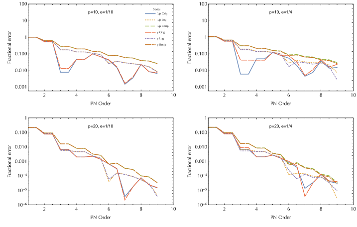
Figure 1: Accuracy of the spin-precession invariant PN expansion and its resummations for several individual orbits. The numerical values of our redshift expansion are plotted against data from Akcay et al. (2017) for the orbits $(p=10,e=1/10),(p=10,e=1/4),(p=20,e=1/10),(p=20,e=1/4)$. Within each plot comparisons are made for both the $1/p$ and $y$ expansions, both with and without the use of logarithmic and reciprocal summations. Note the changes in vertical scaling in the bottom two plots.

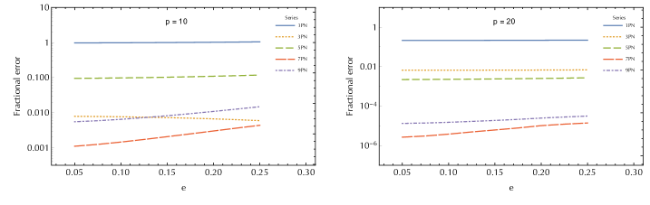
Figure 2: Accuracy of the spin invariant PN expansion with increasing $e$. The (simple) $1/p$ expansion is compared to numerical data for the $e$ values $0.05$ to $25$ at $0.05$ intervals (plots are made continuous for clarity) for both $p=10$ and $p=20$.

All of the series exhibit fairly strong convergence for the case $p=20$, reaching a fractional error better than $10^{-5}$ for both $e=0.1$ and $e=0.25$ using 9PN terms. The dataset in Akcay et al. (2017) is restricted to $e\leq 0.25$, limiting our ability to test the expansions at higher eccentricities. The experience with numerical comparisons of the redshift invariant Munna and Evans (2022) suggests that our series will remain viable up to $e\simeq 0.5$ at $p=20$. At the closer separation of $p=10$ the convergence is markedly slower, attaining relative errors near $1\%$ at both $e=0.1$ and $e=0.25$. This observation is consistent with the analysis in Bini et al. (2018), who showed that the series is expected to diverge at a larger radius than the redshift invariant (i.e., at the separatrix, as opposed to the light ring). Moreover, the basic resummation methods we have tried have not substantially improved the convergence.

Fig. 2 shows how the fractional errors behave versus eccentricity $e$ when using a set of series that have been truncated at different PN orders. We see that knowledge gained from our calculation of the spin-precession invariant through $e^{16}$ provides series that converge uniformly over a range of eccentricity through $e=0.25$. The curves strongly suggest that our PN series will remain accurate as $e\rightarrow 0.5$ or more. The current version of our code could reach higher PN order but at the expense of reducing the order of the expansion in $e$, for example perhaps reaching 12PN and $e^{10}$. In any event, if we consider the task of modeling EMRIs, conservative dynamical effects are suppressed by a factor of the mass ratio relative to the secular effect of the gravitational wave fluxes Hinderer and Flanagan (2008). Thus, our present depth of PN expansion of the spin-precession invariant is likely adequate for giving its contribution to EMRI dynamics.

V Conclusions

We have presented the PN and eccentricity expansion of the spin-precession invariant $\psi$ at first order in the mass ratio for a point mass in bound eccentric motion about a Schwarzschild black hole. The RWZ formalism is used, calculating the metric perturbation and self-force in Regge-Wheeler gauge. The calculation is completely analytic, using a Mathematica code and drawing upon the analytic PN expansion of the MST formalism and the general-$l$ expansion ansatz of Bini and Damour (2013); Kavanagh et al. (2015). The construction and regularization of the spin-precession invariant follows methods used by Akcay et al. (2017); Kavanagh et al. (2017); Bini et al. (2018), as well as simplifications of the eccentricity dependence developed in our previous work Munna (2020); Munna and Evans (2022). We have computed the spin-precession invariant to 9PN (which has been done before Bini et al. (2018); Bini and Geralico (2019)) but have calculated the eccentricity expansion to $e^{16}$ (with one exception, 4PN, which is calculated to $e^{30}$), far beyond the order $e^{2}$ results previously known.

The high-order eccentricity expansions led to the discovery of five new closed-form expressions, for $\Delta\psi_{4L}$, $\Delta\psi_{5L}$, $\Delta\psi_{6L}$, $\Delta\psi_{7L2}$, and $\Delta\psi_{8L2}$. In addition, we were able to use the methods developed in our past work on the gravitational wave fluxes Munna and Evans (2019); Munna et al. (2020); Munna and Evans (2020) and the redshift invariant Munna and Evans (2022) to segregate the eccentricity dependence of many of the other PN terms into significant functional parts and to identify eccentricity singular factors that aid convergence in the $e\rightarrow 1$ limit. The PN series results were compared to prior numerical calculations, and shown to exhibit fractional errors in convergence of around $10^{-5}$ for orbital separation of $p=20$ and of around $10^{-2}$ for $p=10$.

The expansions of $\Delta\psi$ could be extended further. The bottleneck step in the calculation is the expansion of the general-$l$, even-parity normalization constant $C_{lmn}^{+}$, which requires about 7 days on the UNC Longleaf cluster to reach 10PN (relative) order and $e^{20}$. Beyond simply committing more resources or finding a faster cluster, intermediate expansions, which sacrifice PN order for higher order in eccentricity or vice versa, can be obtained immediately and may be useful. As we described, by focusing on one PN order (4PN), we were able to push the eccentricity expansion to $e^{30}$.

It will be useful now to translate these expansions to their equivalent quantities within the EOB formalism. EOB waveforms have been crucial to the success of LIGO data analysis and will likely contribute to deciphering LISA detections. The spin-precession invariant in first-order self-force calculations can be transcribed to yield portions of the EOB gyrogravitomagnetic ratio $g_{S*}(1/r;p_{r};p_{\varphi})$, by extending a procedure described in Kavanagh et al. (2017). However, the process is lengthy, with each new order in $e^{2}$ requiring cumbersome derivations, and we leave that process for future work.