Pion distribution amplitude at the physical point using the leading-twist expansion of the quasi-distribution-amplitude matrix element

Abstract

We present a lattice QCD determination of the distribution amplitude (DA) of the pion and the first few Mellin moments from an analysis of the quasi-DA matrix element within the leading-twist framework. We perform our study on a HISQ ensemble with $a=0.076$ fm lattice spacing with the Wilson-clover valence quark mass tuned to the physical point. We analyze the ratios of pion quasi-DA matrix elements at short distances using the leading-twist Mellin operator product expansion (OPE) at the next-to-leading order and the conformal OPE at the leading-logarithmic order. We find a robust result for the first non-vanishing Mellin moment $\langle x^{2}\rangle=0.287(6)(6)$ at a factorization scale $\mu=2$ GeV. We also present different Ansätze-based reconstructions of the $x$-dependent DA, from which we determine the perturbative leading-twist expectations for the pion electromagnetic and gravitational form-factors at large momentum transfers.

I Introduction

The study of inclusive deep-inelastic processes by describing them using process-independent parton distribution functions (PDFs) has resulted in a good understanding of collinear internal structures of hadrons. The next generation of experimental facilities (e.g., Aguilar et al. (2019); Arrington et al. (2021); Adams et al. (2018a, b)) will focus on observables that characterize hard semi-inclusive and exclusive processes to relate intrinsic properties of hadrons to those of the partons. The generalized parton distribution functions (GPDs) and the meson distribution amplitudes (DAs) will play crucial roles as universal soft-functions in the descriptions of exclusive reactions in hard kinematical regimes through factorization. Thus, non-perturbative determination of such parton distributions and amplitudes are currently essential.

Concretely, the pion DA, $\phi(x)$, captures the overlap of the pion with a state with two collinear valence quarks carrying fractions $x$ and $(1-x)$ of the pion light-front momentum $P^{+}$ Lepage and Brodsky (1980, 1979); Efremov and Radyushkin (1980). Hence, the pion DA is of theoretical interest due to its proximity to being the light-front wave-function Lepage and Brodsky (1979) of the Nambu-Goldstone boson of chiral symmetry breaking; by comparison with DAs of non-Goldstone pseudoscalar mesons, one could learn about how the fundamental quark-gluon interaction leads to the special properties of the pion (see review Roberts et al. (2021), and Ref. Gao et al. (2021a) for our lattice calculation in a related direction). Phenomenologically, the properties of the pion DA, such as its shape and its Mellin moments, are still not precisely known and the main experimental input has been from the factorization of the pion-photon transition form factor Behrend et al. (1991); Gronberg et al. (1998); Aubert et al. (2009); Uehara et al. (2012); Melic et al. (2003); Gao et al. (2022a), and from past Dally et al. (1981, 1982); Amendolia et al. (1984, 1986); Volmer et al. (2001); Tadevosyan et al. (2007); Huber et al. (2008); Blok et al. (2008) (and ongoing Dudek et al. (2012)) investigations of the large-$Q^{2}$ behavior of the pion electromagnetic form factor Efremov and Radyushkin (1980); Farrar and Jackson (1979); Lepage and Brodsky (1980). From a field-theoretic standpoint, the determination of the pion DA involves the light-front correlation Radyushkin (1977); Efremov and Radyushkin (1980); Lepage and Brodsky (1980),

$$\phi(x,\mu)=\int\frac{d\lambda}{2\pi}e^{-i\frac{x}{2}\lambda}{\cal I}(\lambda,\mu),\ {\rm with}\ \lambda=P^{+}z^{-},$$ (1)

with a dimensionless invariant amplitude ${\cal I}$ renormalized in the ${\overline{\mathrm{MS}}}$ scheme at scale $\mu$ defined as,

$$if_{\pi}P^{+}{\cal I}(\lambda,\mu)=\matrixelement{0}{\overline{d}(-z^{-}/2)\gamma^{+}\gamma_{5}W_{+}u(z^{-}/2)}{\pi^{+};P},$$ (2)

where $W_{+}$ is a straight Wilson line from $-z^{-}/2$ to $z^{-}/2$ along the light-cone. Various model-based determinations (e.g., Chernyak and Zhitnitsky (1982); Bakulev et al. (2001); Agaev et al. (2011); Chang et al. (2013a); Ruiz Arriola and Broniowski (2006)) of $\phi$ have given key insights into the full $x$-dependence and the moments. For a rigorous QCD-based non-perturbative calculation, one needs to rely on lattice QCD computation. However, the unequal time-separation in the above light-front correlator has prevented a direct computation of DA.

The first few Mellin and Gegenbauer moments of the pion DA have been computed from leading-twist local operators on the lattice Kronfeld and Photiadis (1985); Martinelli and Sachrajda (1987); DeGrand and Loft (1988); Daniel et al. (1991); Del Debbio et al. (2000, 2003); Braun et al. (2006); Arthur et al. (2011); Braun et al. (2015); Bali et al. (2017, 2019). The difficulty of this approach is the nontrivial renormalization of these operators on the lattice, which limits the number of lowest calculable moments. One way to avoid this challenge is through a leading-twist expansion of the pion-to-vacuum transition matrix element of certain spatially separated operators Braun and Müller (2008). The short-distance logarithmic divergences are absorbed as part of perturbatively computed Wilson coefficients, and most importantly, the expansion coefficients are proportional to the moments of the DA. Such a leading-twist expansion approach was first applied using the pion-to-vacuum transition matrix element using two current operator insertions Braun and Müller (2008), which has been been utilized in further studies of DA and the moments Bali et al. (2018a, b). Analogous real-space analysis using current-current correlators was also applied to the pion-to-pion forward matrix element to determine the pion PDF Ma and Qiu (2018); Sufian et al. (2019, 2020). Besides, there are also approaches based on the leading-twist expansion of current-current correlators in the Fourier space Chambers et al. (2017), including the method that uses an intermediate heavy quark Detmold and Lin (2006); Detmold et al. (2021, 2022), to calculate the higher moments of DAs and PDFs.

Recently, there have been new advancements in the determination of parton distribution functions using multiplicatively renormalized, spatially-extended quark-antiquark operators based on the LaMET Ji (2013, 2014); Ji et al. (2021a) and the pseudodistribution Radyushkin (2017); Orginos et al. (2017); Radyushkin (2020) approaches. For example, Refs. Izubuchi et al. (2019); Gao et al. (2020); Lin et al. (2021); Gao et al. (2022b) are recent computations of the pion PDF using the bilocal quark-antiquark operator. For DA, one can construct the pion-to-vacuum transition matrix element of such a bilocal quark-antiquark operator Ji et al. (2015), which we simply refer to as the quasi-DA matrix element. The aim of this paper is to apply the leading-twist expansion of the quasi-DA matrix element in a manner similar to Ref Braun and Müller (2008), to extract the Mellin moments of the pion DA, and attempt to reconstruct the shape of the pion DA based on strategies utilized in the case of PDFs. Previously, such quasi-DA matrix elements of both the pion and kaon have been investigated using the $x$-space LaMET matching Zhang et al. (2017, 2019); Liu et al. (2019); Zhang et al. (2020); Hua et al. (2022). Due to the differences in the renormalization method and the analysis methodology for a leading-twist expansion approach, we expect this work to shed new light into the quasi-DA method as a way to obtain the pion DA and its moments. Apart from the above leading-twist expansion or effective theory matching approaches, it has also been proposed to directly obtain the structure functions from the hadronic tensor on the lattice through a nontrivial inversion of Euclidean correlators Liu and Dong (1994), which has not yet been applied to the extraction of DAs.

The plan of the paper is as follows. First, we give an overall description of our methodology in Section II. Then, in Section III, we present the perturbative results pertaining to conformal and Mellin OPEs. In Section IV, we give the details of our lattice calculation. In Section V, we present the details of the determinations of the bare quasi-DA matrix element and the renormalized ratios thereof. In Section VI, we present the results on the pion DA; here, we first present the analysis specifications, then we present the Mellin moments for fixed spatial distances, after which we present our model-independent determination of the first two Mellin moments, and finally, we describe the model-dependent reconstructions of the shape of the pion DA. From such reconstructed $x$-dependent DA, we present the perturbative expectations for pion form-factors at large momentum transfers. In Section VII, we summarize our findings.

II Method

We specify four-vectors as $v_{\rho}$, whose components are $(v_{0},v_{1},v_{2},v_{3})$ with $v_{0}$ being the temporal component, and $\mathbf{v}=(v_{1},v_{2},v_{3})$ as the spatial component. We use the $\rho=3$ direction for spatial separations and as the direction of the pion momentum. The metric convention is $v\cdot w=v_{0}w_{0}-\mathbf{v}\cdot\mathbf{w}$. We specify the Dirac $\gamma$-matrices as $\gamma_{\rho}$, and we use the Minkowskian convention for them. For the ease of understanding, we specify them as $(\gamma_{t},\gamma_{x},\gamma_{y},\gamma_{z})$ respectively, when explicitly mentioning a matrix. We specify the bare and renormalized quantities using superscript “B” and “R” respectively.

We use the short-distance behavior of the quasi-DA matrix element of a boosted pion, $\pi^{+}(u\bar{d})$, to determine its leading-twist DA. The quasi-DA operator is the equal-time bilocal quark bilinear operator,

$$O^{B}_{\rho}(z)=\overline{d}(-z/2)\gamma_{\rho}\gamma_{5}W_{-z/2,z/2}u(z/2),$$ (3)

with the straight Wilson-line $W_{-z/2,z/2}$ connecting the quark and antiquark that are separated spatially as $z=(0,0,0,z_{3})$. At non-zero $z$, the operator suffers from a linear divergence in the self-energy of the Wilson-line, $e^{-c|z|}$, and also from the end-point logarithmic divergence, and therefore, it needs to be renormalized. Thus the operator above is bare, and hence, the superscript $B$ to specify this. Let $O_{\rho}^{R}(z,\mu)$ be the renormalized operator in the ${\overline{\mathrm{MS}}}$ scheme at scale $\mu$. The quasi-DA matrix element for the pion is,

$$iP_{\rho}h^{R}\left(z\cdot P,z^{2},\mu\right)\equiv\matrixelement{0}{O^{R}_{\rho}(z,\mu)}{\pi^{+};P},$$ (4)

with the on-shell pion momentum $P=(E(P_{3}),0,0,P_{3})$. The Lorentz invariant $\lambda=-z\cdot P=z_{3}P_{3}$ is called the Ioffe-time or light-cone distance in the literature. We note that the left-hand side of the above equation is not a Lorentz decomposition, instead we have defined $h$ above in a form convenient for the leading-twist expansion that is proportional to $P_{\rho}$ . As a specific case, $z_{3}=0$ and for all momentum $P_{3}$, the local operator $O^{R}_{\rho}(0)$ is the axial-current operator, and $h(z_{3}=0,P_{3})=f_{\pi}$, the pion decay constant.

The idea used in this paper is that for quark-antiquark separations $z_{3}$ that are small in QCD scales and for momenta $P_{3}>0$, one can describe the $\lambda$ and $z^{2}$ dependencies of $h^{R}(\lambda,z^{2},\mu)$ within a leading-twist OPE framework valid up to higher-twist contributions. This lets us relate the lattice-calculable equal-time quantity $h^{R}(\lambda,z^{2})$ to the light-cone distribution amplitude $\phi(x,\mu)$ at a factorization scale $\mu$ and its Mellin moments,

$$\langle x^{n}\rangle=\int_{-1}^{1}\phi(x,\mu)x^{n}dx.$$ (5)

The framework is similar to the one used in the determination of the parton distribution functions (PDFs), however, the key difference for the case of DA is that the matrix element in Eq. (4) is between the boosted pion state and vacuum state. This results in a different leading-twist expansion than in the case of the forward matrix element for PDFs. As we will show in the paper, the leading-twist expansion of $h^{R}(\lambda,z^{2},\mu)$ for DA is

$$h^{\rm tw2}(\lambda,z^{2},\mu)=\sum_{n=0}\frac{(-i\lambda/2)^{n}}{n!}\sum_{m=0}^{n}C_{n,m}(z^{2}\mu^{2})\langle x^{m}\rangle,$$ (6)

where $C_{n,m}(\mu^{2}z^{2})$ are the Wilson coefficients calculable in perturbation theory that relates $h$ to the DA via its Mellin moments at scale $\mu$. By the superscript “tw2” we mean that the expansion ignores all terms with twists bigger than two. Henceforth, we will refer to Eq. (6) as the Mellin OPE (M-OPE). In Section III, we provide the NLO results for $C_{n,m}$ for $O^{R}_{3}$. Under an ERBL Lepage and Brodsky (1980, 1979); Efremov and Radyushkin (1980) evolution in $\mu$, the different Mellin moments mix, which is also reflected in the non-vanishing off-diagonal nature of $C_{n,m}$. At the level of leading logarithms and up to finite ${\cal O}(\alpha_{s})$ corrections, massless QCD is conformal and this helps in diagonalizing the leading-twist expansion (see review Braun et al. (2003)) with respect to evolution. Such an expansion in terms of the conformal partial waves ${\cal F}_{n}(\lambda/2,\mu^{2}z^{2};\alpha_{s})$ is given as

$$h^{\rm tw2}(\lambda,z^{2},\mu)=\sum_{n=0}a_{n}(\mu){\cal F}_{n}(\lambda/2,z^{2}\mu^{2};\alpha_{s}),$$ (7)

where $a_{n}$ are the Gegenbauer moments at scale $\mu$, and they satisfy the simpler LO DGLAP evolution. In Section III, we provide the expressions for ${\cal F}_{n}$. We will refer to Eq. (7) as the conformal OPE (C-OPE).

At next-to-leading order, the Mellin and Conformal OPEs differ in the finite $\alpha_{s}$ terms and are the same up to $\alpha_{s}^{0}$ and $\alpha_{s}\log(z^{2}\mu^{2})$ terms. At the level of practical implementation, we have to truncate Eq. (6) and Eq. (7) — for C-OPE, it is a truncation in conformal partial waves that each have infinite order in $\lambda$, whereas for M-OPE, it is a truncation in the order of $\lambda$. We will use M-OPE primarily in this paper to implement the matching at NLO, and compare the results with that obtained with C-OPE to cross-check that the results are approximately the same. The expressions in Eq. (6) and Eq. (7) are general for any pseudoscalar mesons, but it gets further simplified for the pion; due to isosopin symmetry, the Mellin and Gegenbauer moments for odd $n$ vanish, and therefore, at leading-twist the matrix elements are purely real. We will use this fact in our analysis and set odd $n$ moments to zero. Since the Gegenbauer moments for all $n>0$ approach zero under evolution to $\mu\to\infty$, the C-OPE expression simply approaches ${\cal F}_{0}(\lambda/2)$ asymptotically.

In the above discussion, we assumed that the operator is renormalized in the ${\overline{\mathrm{MS}}}$ scheme, which cannot be directly implemented on the lattice. Furthermore, it was shown in Refs. Constantinou and Panagopoulos (2017); Chen et al. (2018), that the operator $O^{B}_{3}(z)$, that has the $\gamma_{z}\gamma_{5}$ structure, is multiplicatively renormalizable, whereas the choice $O^{B}_{0}(z)$ that has the $\gamma_{t}\gamma_{5}$ structure, mixes with the $\bar{u}\gamma_{5}\gamma_{z}\gamma_{t}d$ operator when lattice-regulated fermions that break chiral-symmetry are used. Therefore, in this work, we only work with the $O^{B}_{3}(z)$ operator to avoid the mixing. We adapt the renormalization group invariant (RGI) ratios Orginos et al. (2017); Fan et al. (2020); Gao et al. (2020) of hadronic matrix elements for the renormalization. Since the renormalization of $O^{B}_{3}(z)$ is purely multiplicative, the ratio,

$${\cal M}(\lambda,z^{2},P^{0})\equiv\frac{h^{B}(\lambda,z_{3}^{2})}{h^{B}(\lambda_{0},z_{3}^{2})}=\frac{h^{R}(\lambda,z_{3}^{2},\mu)}{h^{R}(\lambda_{0},z_{3}^{2},\mu)},\ \lambda_{0}=P_{3}^{0}z_{3},$$ (8)

with respect to the matrix element at a fixed momentum $P^{0}$ is an RGI quantity that we can determine on the lattice. We obtain the leading twist expression for ${\cal M}$ from the ${\overline{\mathrm{MS}}}$ expressions for $h^{\rm tw2}$ in Eq. (6) and Eq. (7) by making use of its RGI nature as

$${\cal M}^{\rm tw2}(\lambda,z^{2},P^{0})=\frac{h^{\rm tw2}(\lambda,z^{2},\mu)}{h^{\rm tw2}(\lambda_{0},z^{2},\mu)}.$$ (9)

The actual lattice data in the range of $z_{3}$ and $P_{3}$ that we use could suffer from lattice corrections and higher-twist corrections to the continuum leading-twist expressions in Eq. (6) and Eq. (7). We model the two corrections using some functions $L(z,P,a)$ and $H(z,P)$ respectively. With such corrections, we use expressions of the type,

$${\cal M}^{\rm tw2,corr}(\lambda,z^{2},P^{0})=$$ (10)

$$\qquad\frac{h^{\rm tw2}(\lambda,z^{2},\mu)+L(z,P,a)+H(z,P)}{h^{\rm tw2}(\lambda_{0},z^{2},\mu)+L(z,P^{0},a)+H(z,P^{0})},$$ (11)

to perform our fits to the lattice QCD data for ${\cal M}(\lambda,z^{2},P^{0})$ to obtain information on the Mellin or Gegenbauer moments of the DA depending on whether M-OPE or C-OPE is used for $h^{\rm tw2}$, respectively. Equivalently, by modeling the functional form of $\phi(x,\mu)$, we also reconstruct the $x$ dependence of the pion DA. Alternatively, from such analyses, we can also infer the ${\overline{\mathrm{MS}}}$ light-front Ioffe-time distribution (ITD) as

$${\cal I}(\lambda,\mu)=\sum_{n=0}\frac{(-i\lambda/2)^{n}}{n!}\langle x^{n}\rangle(\mu).$$ (12)

We discuss the implementation of the above set of steps further in the following sections presenting our results.

III Analytical results for conformal and Mellin OPE

III.1 Short distance factorization of the quasi-DA matrix element

In $x$-space, the quasi-DA can be perturbatively matched onto the light-cone DA at large momentum, where the matching coefficient has been derived in the $\overline{\rm MS}$ scheme at one-loop order Liu et al. (2019). In coordinate space, the quasi-DA matrix element $h(\lambda,z^{2},\mu^{2})$ can also be perturbatively matched onto the light-cone correlation ${\cal I}(\lambda,\mu)$ through a short-distance factorization formula, which has been derived in QCD at one-loop order Radyushkin (2019) as

$$h^{R}(\lambda,z^{2},\mu^{2}) =\int_{0}^{1}dw\ C(w,\lambda,z^{2}\mu^{2}){\cal I}(w\lambda,\mu)$$

$$\qquad+{\cal O}(z^{2}\Lambda_{\rm QCD}^{2})\,,$$ (13)

where the matching kernel

$$C(w,\lambda,z^{2}\mu^{2})$$

$$=\delta(\bar{w})+{\alpha_{s}C_{F}\over 2\pi}\Bigg{\{}2\left({\mathbf{L}}+1\right)\delta(\bar{w})+\big{(}{\mathbf{L}}+1\big{)}$$

$$\quad\times\left[-\left({2w\over\bar{w}}\right)_{+}\cos({\bar{w}\lambda\over 2})-{\sin(\bar{w}\lambda/2)\over\lambda/2}\right]$$

$$-4\left({\ln\bar{w}\over\bar{w}}\right)_{+}\cos({\bar{w}\lambda\over 2})+{(2+2\delta_{\rho 3})\sin(\bar{w}\lambda/2)\over\lambda/2}\Bigg{\}}$$

$$\quad+{\cal O}(\alpha_{s}^{2})\,,$$ (14)

with $C_{F}=4/3$, ${\mathbf{L}}=\ln(z^{2}\mu^{2}e^{2\gamma_{E}}/4)$, and $\bar{w}=1-w$. The $2\delta_{\rho 3}$ term in the curly bracket can be inferred from the factorization of the forward quasi-PDF matrix elements Izubuchi et al. (2018).

III.2 Conformal OPE

The LCDA can be expressed as the sum of Gegenbauer moments,

$$\phi(x,\mu) ={3\over 4}(1-x^{2})\sum_{\begin{subarray}{c}n=0,\\ \rm even\end{subarray}}^{\infty}{\cal C}_{n}^{3\over 2}(x)a_{n}(\mu)\,,$$ (15)

where ${\cal C}_{n}^{3\over 2}(x)$ is a Gegenbauer polynomial (refer (DLMF, , Table 18.3.1)). The Gegenbauer moment $a_{n}(\mu)$ can also be projected from $\phi(x,\mu)$ as

$$a_{n}(\mu)={4(n+3/2)\over 3(n+1)(n+2)}\int_{-1}^{1}dx\ \phi(x,\mu){\cal C}_{n}^{3\over 2}(x)\,.$$ (16)

At leading logarithmic (LL) accuracy, QCD is conformal, and $\phi_{n}(\mu)$ evolves multiplicatively with the anomalous dimension

$$\gamma_{n}(\alpha_{s}) ={\alpha_{s}C_{F}\over 4\pi}\gamma_{n}^{(0)}+{\cal O}(\alpha_{s}^{2})$$ (17)

$$={\alpha_{s}C_{F}\over 4\pi}\left[4H_{n+1}-{2\over(n+1)(n+2)}-3\right]+{\cal O}(\alpha_{s}^{2}),$$

with $H_{n}=\sum_{i=1}^{n}1/i$. The value of $\gamma_{n}$ is different from that for the Mellin moments of PDFs by a minus sign. Therefore, the Gegenbauer moments should be the basis of OPE under the conformal approximation to QCD.

The conformal OPE of the quasi DA matrix element in the $\overline{\rm MS}$ scheme can be inferred from that for the current-current correlator Braun and Müller (2008) as

$$h^{\rm tw2}_{\rm cf}(\lambda,z^{2},\mu^{2}) =\sum_{\begin{subarray}{c}n=0,\\ \rm even\end{subarray}}^{\infty}{\cal F}_{n}({\lambda\over 2},z^{2}\mu^{2};\alpha_{s})a_{n}(\mu)\,,$$ (18)

where $\lambda=zP^{z}$, and the LL resummed coefficient

$${\cal F}_{n}(\lambda,z^{2}\mu^{2};\alpha_{s}) =c_{n}(\alpha_{s})(\mu^{2}z^{2})^{{\gamma_{n}}+\gamma_{O}}{\Gamma(2-{\gamma_{n}})\Gamma(1+n)\over\Gamma(1+n+{\gamma_{n}})}$$

$$\quad\times{3\over 4}\ i^{n}\sqrt{\pi}{(n+1)(n+2)\over 2}{\Gamma(n+\gamma_{n}+{5\over 2})\over\Gamma(n+{5\over 2})}$$

$$\quad\times\Big{(}{\lambda\over 2}\Big{)}^{-{3\over 2}-\gamma_{n}}J_{n+\gamma_{n}+{3\over 2}}(\lambda)\,.$$ (19)

with $\Gamma$ and $J_{n}$ being the standard gamma function and Bessel function of first-kind respectively, and

$$c_{n} =1+{\alpha_{s}C_{F}\over 2\pi}\Bigg{[}{5+2n\over 2+3n+n^{2}}+{2\delta_{\rho 3}\over 2+3n+n^{2}}$$

$$\qquad+2(1-H_{n})H_{n}-2H_{n}^{(2)}\Bigg{]}+{\cal O}(\alpha_{s}^{2})\,,$$ (20)

which is the same as the Wilson coefficients in the OPE of the helicity quasi PDF matrix elements Izubuchi et al. (2018), and

$$\gamma_{O} =\gamma_{O}^{(0)}+{\cal O}(\alpha_{s}^{2})={\alpha_{s}C_{F}\over 4\pi}\cdot{3}+{\cal O}(\alpha_{s}^{2})\,,$$ (21)

which is the anomalous dimension of the nonlocal operator $O_{\rho}(z,\mu)$. Note that in Eq. (19) the running of strong coupling is turned off because we assumed conformal symmetry.

III.3 OPE in terms of Mellin moments

If we do not include the scale evolution in the OPE, then we can consider expansion in terms of the Mellin moments in Eq. (6). The coefficient functions

$$C_{n,m} =C^{(0)}_{n,m}+{\alpha_{s}C_{F}\over 2\pi}C^{(1)}_{n,m}+{\cal O}(\alpha_{s}^{2})$$ (22)

can be obtained by the relation

$$C^{(0)}_{n,m}=\delta_{n,m}\,,$$ (23)

$$\sum_{m=0}^{n}C^{(1)}_{n,m}(z^{2}\mu^{2})x^{m}$$

$$=2\big{(}{\mathbf{L}}+1\big{)}x^{n}+\big{(}{\mathbf{L}}+1\big{)}\int_{0}^{1}dw$$

$$\qquad\times\left[\left({-2w\over\bar{w}}\right)_{+}{(xw-\bar{w})^{n}+(xw+\bar{w})^{n}\over 2}\right.$$

$$\qquad\qquad\left.-{-(xw-\bar{w})^{n+1}+(xw+\bar{w})^{n+1}\over 2(n+1)}\right]$$

$$+\int_{0}^{1}dw\left[\left(-{4\ln\bar{w}\over\bar{w}}\right)_{+}{(xw-\bar{w})^{n}+(xw+\bar{w})^{n}\over 2}\right.$$

$$\quad\left.+(2+2\delta_{\rho 3}){-(xw-\bar{w})^{n+1}+(xw+\bar{w})^{n+1}\over 2(n+1)}\right]\,,$$ (24)

where $C^{(1)}_{n,m}$ can be read off from the coefficients of $x^{m}$. The lowest few coefficient functions are

$$C_{0,0}^{(1)} ={3\over 2}{\mathbf{L}}+{7\over 2}\,,$$ (25)

$$\sum_{m=0}^{n}C^{(1)}_{1,m}(z^{2}\mu^{2})x^{m} =\left({17\over 6}{{\mathbf{L}}}-{1\over 2}\right)x\,,$$ (26)

$$\sum_{m=0}^{n}C^{(1)}_{2,m}(z^{2}\mu^{2})x^{m} =\left(\frac{43}{12}{\mathbf{L}}\!-\!\frac{37}{12}\right)x^{2}\!+\!\frac{11}{12}\!-\!\frac{5}{12}{\mathbf{L}}\,,$$ (27)

$$\sum_{m=0}^{n}C^{(1)}_{3,m}(z^{2}\mu^{2})x^{m} =\left(\frac{247}{60}{\mathbf{L}}-\frac{923}{180}\right)x^{3}$$

$$\qquad\qquad+\left(\frac{79}{60}-\frac{11}{20}{\mathbf{L}}\right)x\,,$$ (28)

$$\sum_{m=0}^{n}C^{(1)}_{4,m}(z^{2}\mu^{2})x^{m} =\left(\frac{68}{15}{\mathbf{L}}-\frac{247}{36}\right)x^{4}$$ (29)

$$\qquad+\left(\frac{5}{3}-\frac{19}{30}{\mathbf{L}}\right)x^{2}+\frac{1}{4}-\frac{2}{15}{\mathbf{L}}\,.$$

IV Computational setup

We used a mixed fermion action setup consisting of a 2+1 flavor HISQ sea quark action and a clover-improved Wilson fermion action for the valence quarks. The HISQ ensemble Bazavov et al. (2019) was generated by the HotQCD collaboration, and consists of $L_{s}^{3}\times L_{t}=64^{3}\times 64$ lattice sites at a lattice spacing of $a=0.076$ fm. The sea quark mass in the setup corresponds to a near physical pion mass of 140 MeV. The tadpole improved Wilson clover valence quarks couple to 1-HYP smeared gauge links Hasenfratz and Knechtli (2001). We tuned the Wilson mass to obtain the valence pion mass of 140 MeV. Therefore, both the sea and valence quarks are tuned to the physical point.

In order to compute the quasi-DA matrix element of a pion with momentum $P_{3}$, the two essential ingredients are the $\pi$-$\pi$ and $\pi$-${\cal O}_{3}$ correlators . The pion-pion two-point function at source-sink time separation of $t_{s}$ is

$$C_{\pi\pi}(t_{s},P_{3})=\left\langle\pi(\mathbf{P},t_{s})\pi^{\dagger}(\mathbf{x}_{0},0)\right\rangle,$$ (30)

where

$$\pi^{\dagger}(\mathbf{x},t_{s})=\overline{u}_{s}(\mathbf{x},t_{s})\gamma_{5}d_{s}(\mathbf{x},t_{s}),$$ (31)

with $\pi^{\dagger}(\mathbf{P},t_{s})=\sum_{\mathbf{x}}\pi^{\dagger}(\mathbf{x},t_{s})e^{i\mathbf{P}\cdot\mathbf{x}}$. The $u_{s}$ and $d_{s}$ represent Coulomb-gauge Gaussian smeared quark operators, with the smearing radius as 0.59 fm. At nonzero spatial momentum $\mathbf{P}=(0,0,P_{3})$, we implemented the boosted quark smearing Bali et al. (2016) with quark boosts, $k_{3}=\pm\zeta P_{3}$, for $u$ and $d$ respectively. The other ingredient, the pion-quasi DA-operator correlator with time separation $t_{s}$, is

$$C_{\pi\tilde{O}_{3}}(t_{s};z_{3},P_{3})=\left\langle\tilde{O}^{B}_{3}(z_{3};\mathbf{P},t_{s})\pi^{\dagger}(\mathbf{x}_{0},0)\right\rangle,$$ (32)

where

$$\tilde{O}^{B}_{3}(z_{3};\mathbf{P},t_{s})=$$

$$\displaystyle\quad\sum_{\mathbf{x}}\overline{d}(\mathbf{x},t_{s})\gamma_{z}\gamma_{5}W(\mathbf{x},t_{s};\mathbf{x}+\mathbf{z},t_{s})u(\mathbf{x}+\mathbf{z},t_{s})e^{-i\mathbf{P}\cdot\mathbf{x}}.$$

(33)

The spatial part of the quark-antiquark separation $z=(0,0,0,z_{3})$ is denoted with $\mathbf{z}$. The straight Wilson-line along the $z$-direction is $W(\mathbf{x},t_{s};\mathbf{x}+\mathbf{z},t_{s})=\prod_{k=0}^{z_{3}/a}U^{\rm HYP}_{3}(\mathbf{x}+ka\hat{z},t_{s})$, where $U^{\rm HYP}$ is the 1-HYP smeared gauge link, the same as those used in the Wilson Dirac operator. The $u$ and $d$ quark operators in Eq. (33) are not Gaussian smeared. One should note that the coordinates of the antiquark and quark are at $x$ and $x+z$ which differs from the one in Eq. (3), and hence the tilde on top of $O_{3}$ to make this distinction clear. This is due to the ease of implementation of the former convention on the lattice, and we defer the conversion to the analysis-wise convenient convention in Eq. (3) at a later stage by multiplying the results with a phase $\exp\left(-iP_{3}z_{3}/2\right)$. We computed the quark propagators that occur in the Wick contractions of Eq. (30) and Eq. (32) on GPUs using the multigrid algorithm Brannick et al. (2008) as implemented in the QUDA suite Clark et al. (2010); Babich et al. (2011); Clark et al. (2016).

We performed the above set of computations at eight different spatial momenta $\mathbf{P}=(0,0,P_{3})$,

$$P_{3}=\frac{2\pi}{L_{s}a}n_{3}\approx 0.254\times n_{3}{\rm\ GeV},$$ (34)

for $n_{3}\in[0,7]$. Thus, the highest momentum we use in this work is $1.78$ GeV which is sufficiently larger than $\Lambda_{\rm QCD}$, and at the same time corresponds to $P_{3}a=0.69$ which is below the lattice-like scales. For these momenta, we decided to choose the phase parameter $\zeta$ in momentum smearing such that $\zeta n_{3}=2$ for $n_{3}\leq 3$ and $\zeta n_{3}=5$ for $n_{3}>3$, so that we could reuse smeared sources for multiple momenta to balance the computational cost and the signal-to-noise ratios.

We used 350 statistically independent configurations. We effectively increased the statistics many folds using the all-mode averaging method Shintani et al. (2015), implemented using exact inversions of the Dirac operator at $N_{\rm ex}$ source locations $\mathbf{x}_{0}$, and sloppy inversions at $N_{\rm sl}$ source locations. For $n_{3}\leq 3$, we used $(N_{\rm ex},N_{\rm sl})=(4,80)$, and for $n_{3}>3$, we used $(8,160)$.

V Determination of matrix element

In this section, we discuss the details of the determination of the ground-state matrix elements of the bare quasi-DA operator at different momenta and quark-antiquark separations, and the RGI ratios that we construct from them.

V.1 Bare matrix element

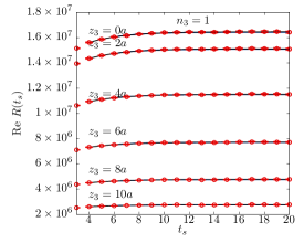
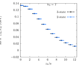
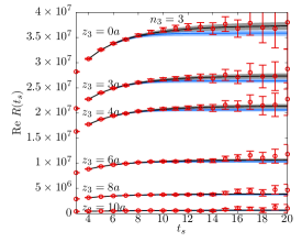
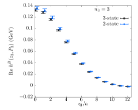
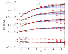
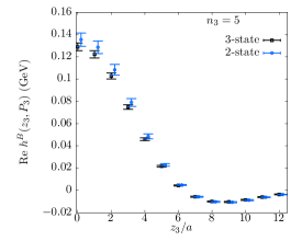
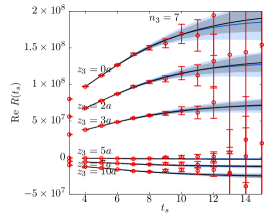
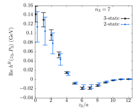
Figure 1: The determination of the real part of the bare matrix element ${\rm Re}\>\tilde{h}^{B}(z_{3},P_{3})$ from two-state and three-state fits to the ratio $R(t_{s})$ for momenta $P_{3}=0.254n_{3}$ GeV for $n_{3}=$ 1, 3, 5 and 7 from top to bottom. The left panels show the extrapolations in $t_{s}$ with the two-state and three-state fits shown as the blue and black bands. The results at different representative values of $z_{3}$ used in this work are also shown together. The right panels show the resulting extrapolated values of ${\rm Re}\>h^{B}(z_{3},P_{3})$, in units of GeV, as a function of $z_{3}/a$. The results using two-state and three-state fits are slightly displaced horizontally for clarity.

We used the spectral decomposition of $C_{\pi\pi}(t_{s};P_{3})$ and $C_{\pi\tilde{O}_{3}}(t_{s};P_{3},z_{3})$ to extract the bare quasi-DA matrix element. That is, the pion-pion correlator,

$$C_{\pi\pi}(t_{s})=\sum_{i=0}^{N_{\rm st}-1}\frac{|Z_{n}|^{2}}{2E_{n}}\left(e^{-E_{n}t_{s}}+e^{-E_{n}(L_{t}-t_{s})}\right),$$ (35)

and the pion-quasiDA correlator,

$$C_{\pi O_{3}}(t_{s})=$$ (36)

$$\qquad\sum_{i=0}^{N_{\rm st}-1}\frac{Z_{n}}{2E_{n}}\matrixelement{0}{\tilde{O}^{B}_{3}(z)}{E_{n}}\left(e^{-E_{n}t_{s}}+e^{-E_{n}(L_{t}-t_{s})}\right),$$

(37)

where the kets are relativistically normalized, and $Z_{n}=\matrixelement{\pi;P_{3}}{\pi^{\dagger}(P_{3})}{0}$, which we assume to be real and positive in this work. The summations in Eq. (35) and Eq. (37) run over all the eigenstates at definite momentum $P_{3}$. However, for practical considerations, one truncates them including only the lowest $N_{st}$ states. We refer to the $N_{\rm st}=2$ truncated expression as the two-state ansatz, and the $N_{\rm st}=3$ truncation as the three-state ansatz. The periodicity of the two correlators is imposed above; for $C_{\pi\tilde{O}_{3}}(t_{s})$ the periodicity can be seen by reflection $(x_{0},x_{1},x_{2},x_{3})\to(-x_{0},-x_{1},-x_{2},x_{3})$, along with $q\to\gamma_{z}q$, $\bar{q}\to\bar{q}\gamma_{z}$ where $q$ is either $u$ or $d$, which is a symmetry of the Euclidean path integral, and therefore, $C_{\pi\tilde{O}_{3}}(t_{s})=C_{\pi\tilde{O}_{3}}(-t_{s})$. We obtained the bare quasi-DA matrix element from the analysis of the ratio,

$$R(t_{s})=\frac{-iC_{\pi\tilde{O}_{3}}(t_{s};P_{3},z_{3})}{C_{\pi\pi}(t_{s};P_{3})},$$ (38)

whose spectral decomposition is simply the ratio of Eq. (37) and Eq. (35). It can be seen that the leading term for large $t_{s}$ behaves as $R(t_{s})\to P_{3}\tilde{h}^{B}(z_{3},P_{3})/Z_{0}$.

First, we obtained the best fit values of the spectral parameters $E_{n}$ and $Z_{n}$ from the analysis of $C_{\pi\pi}$ correlators. In a previous work Gao et al. (2021b), we discussed our fits to the pion correlator on the same gauge ensemble. In this work, we used the two-state and three-state fits with the ground-state energy fixed to the continuum dispersion, $E_{0}(P_{3})=\sqrt{P_{3}^{2}+m_{\pi}^{2}}$. We chose the fit ranges $t_{s}\in[t_{\rm min},t_{\rm max}]$ for $C_{\pi\pi}(t_{s})$ such that they covered the range used for the subsequent fits to the ratio $R$ to be discussed next. Namely, we used $t_{s}\in[4a,32a]$ for two-state fits and $t_{s}\in[2a,32a]$ for three-state fits. In this way, we obtained good effective values of $E_{n}$ and $Z_{n}$ that best describe the excited state contribution to the ratio $R(t_{s})$ in the range of $t_{s}$ we made use of. However, as observed in Ref. Gao et al. (2021b), the values of $E_{0}$, $E_{1}$ and $E_{2}$ from our final fit choice were within errors of the results when larger $t_{\rm min}$ were used, albeit with noisier determinations. Whereas the value of $E_{1}$ at $P_{3}=0$ is consistent with the pole mass of $\pi(1300)$, the value of $E_{2}$ at $P_{3}=0$ from three-state fits is much higher than expected at 3 GeV. Thus, as noted in Gao et al. (2021b), it is likely that the three-state fit with $E_{2}$ capturing the tower of excited states above $E_{1}$ via a single effective state.

In the next step, we used $(Z_{n},E_{n})$ from two-state and three-state fits on jackknife samples as inputs in our fits to $R(t_{s})$ over ranges $t_{s}\in[t_{\rm min},t_{\rm max}]$ on the same jackknife samples. The fits for $R(t_{s})$ used the above spectral decomposition with fit parameters being the amplitudes $\langle 0|O_{3}|E_{n}\rangle$, and therefore, the fits were linear. We performed these fits to $R(t_{s})$ using two-state and three-state ansatz. For two-state fits to $R$, we chose $t_{\rm min}=6a$, whereas for the three-state fits, we used $t_{\rm min}=4a$. For both two- and three-state fits, we chose the maximum range of the fits $t_{\rm max}=20a$ for momenta $n_{3}\leq 3$ and $t_{\rm max}=15a$ for $n_{3}>3$ to avoid noisier estimates at larger $t_{s}$. In this way, we extrapolated the ratio to $t_{s}\to\infty$ to obtain the bare quasi-DA matrix element $\tilde{h}^{B}(z_{3},P_{3})$.

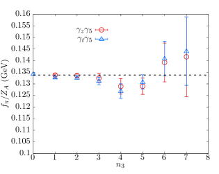
Figure 2: The pion decay constant $f_{\pi}$, modulo the finite renormalization factor $Z_{A}$, is shown as a function of momenta $P_{3}=0.254n_{3}$ that is used in the extraction. The results using $\Gamma=\gamma_{z}\gamma_{5}$ and $\gamma_{t}\gamma_{5}$ are shown in the plot. The dashed curve is the value of $f_{\pi}/Z_{A}$ from $n_{3}=1$.

In Fig. 1, we show some examples from our extrapolations of the real part of $R$. From top to bottom, the data are from momenta $n_{3}=1$, 3, 5 and 7 respectively. Let us first focus on the left panels. We show the data for ${\rm Re}(R)$ as a function of $t_{s}$ for few sample values of $z_{3}$ as specified near the data points. The magnitude of $R$ is not important as it still depends on the two-point function amplitude $Z_{0}$, and only its $t_{s}$ dependence is important here. For $n_{3}=1$ to 3, the variations with $t_{s}$ is smaller due to larger energy gap, $E_{1}-E_{0}$, which is about the gap between pion mass and that of $\pi(1300)$. For larger $n_{3}$, the variation of $R$ with $t_{s}$ is significant due to the states being relativistic. Thus, the extrapolations using spectral decomposition of $R$ is necessary in our calculation, especially in the important large momenta data set. The blue and the black bands show the extrapolations using the two-state and three-state ansatz respectively. Within the statistical errors, the two extrapolation bands satisfactorily describe the $t_{s}$ dependence of the lattice data. However, the three-state fits have a tendency to be closer to the central values of the data when compared to the two-state ones. In the right panels of Fig. 1, we compare the resultant values of the bare quasi-DA matrix element, $\tilde{h}^{B}(z_{3},P_{3})$, from the two-state and three-state fits to $R$ as a function of $z_{3}$. Note that the ordering of blue and black points in the right panel is not in one-to-one correspondence with the left panel as there is also an additional factor $Z_{0}$ that is different between the left and right panels. Within errors, the two-state and three-state extrapolated values are consistent, with perhaps a slight tension in the $n_{3}=3$ momenta. The errors on the three-state fits are comparable or smaller than in the two-state fits due to the $t_{\rm min}$ being $4a$ for three-state ones compared to $6a$ for two-state fits. The relative error at larger momenta $n_{3}>5$ increases at even shorter $z_{3}$. Nevertheless, as we will discuss in the next subsection, the growth in statistical error in shorter $z_{3}$ is reduced due to the RGI ratios that we will construct, and, due to the same reason, even the slightest discrepancies between the two-state and three-state fits seen in the bare matrix element in Fig. 1 will be reduced further. We found similar consistency between the two-state and three-state fits in the case of ${\rm Im}(R)$.

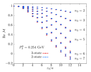
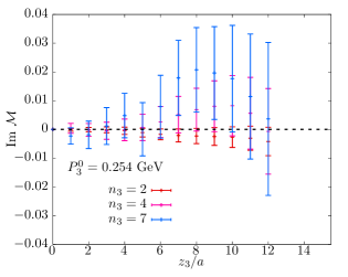
Figure 3: Renormalized matrix elements. The left panel shows the ratio ${\rm Re}\>{\cal M}(z_{3}P_{3},z_{3}^{2},P_{3}^{0})$ as a function of $z_{3}/a$, for a specific $P_{3}^{0}=0.254$ GeV. The results from the two-state and three-state extrapolations are compared in the panel to demonstrate that the ratio further reduces any extrapolation uncertainties. The right panel shows the ratio ${\rm Im}\>{\cal M}(z_{3}P_{3},z_{3}^{2},P_{3}^{0})$ as a function of $z_{3}$ from three different representative momenta. The consistency of ${\rm Im}\>{\cal M}=0$ is demonstrated.

The $z_{3}=0$ value of $\tilde{h}^{B}$ is the bare pion decay constant, $f_{\pi}/Z_{A}$, where $Z_{A}$ is the finite renormalization constant for the axial current operator. Thus $\tilde{h}^{B}(0,P_{3})$ has to be constant with $P_{3}$ if there were no systematical errors in the extrapolations and if ${\cal O}(aP_{3})$ lattice corrections did not affect the lattice results, and therefore, provides a cross-check on our calculation. In Fig. 2, we show $f_{\pi}/Z_{A}$ as a function of momentum $P_{3}$ used in $h^{B}(z_{3}=0,P_{3})$. The red circular data points are the results using the $O_{3}(z=0)$ operator. In addition, we also looked at the local matrix element from $O_{0}(z=0)$. We show those values as the blue triangles in Fig. 2. The values of $f_{\pi}/Z_{A}$ are consistent with being constant with respect to $P_{3}$, with perhaps a slight dip in the central value around $n_{3}=3$, which could be due to statistical fluctuation. The excited state contribution and the Lorentz structure of the $O_{3}$ and $O_{0}$ matrix elements are different, and hence, the consistency between the $f_{\pi}/Z_{A}$ determinations from the two observables is reassuring. Using RI-MOM renormalization procedure, we determined $Z_{A}=0.969(1)$ for the ensemble used in this paper (see Appendix A). From the most precise values of the matrix element at $n_{3}=0$ for $O_{0}(z=0)$ and $n_{3}=1$ for $O_{3}(z=0)$, the values of $f_{\pi}$ from the two observables are 130.0(4) MeV and 129.7(4) MeV respectively. These results agree with the FLAG average for 2+1 flavor QCD $f_{\pi}=130.2(8)$ MeV Aoki et al. (2021). Due to the normalization condition $\langle x^{0}\rangle=1$ that we will impose on the matrix elements, $f_{\pi}$ will not play any further role in this calculation.

V.2 Renormalized ratios

We used the RGI ratios of $h^{B}(z_{3},P_{3})$ to get the renormalized quantities. First, we shifted the location of the operator $\tilde{O}(z)$ by $-z/2$ in order to conform with the definition in Eq. (3). We did this by multiplying $\tilde{h}^{B}(z_{3},P_{3})$ with a phase $\exp(-iz_{3}P_{3}/2)$ from the translation. Next, we improved the ratio in Eq. (8) to impose the condition that the ratio should be exactly unity at $z_{3}=0$ using the so called double ratio procedure. Thus, in the end, we determined the RGI ratio Orginos et al. (2017); Fan et al. (2020); Gao et al. (2020) as

$${\cal M}(\lambda,z^{2},P^{0}) \equiv \left(\frac{\tilde{h}^{B}(z_{3},P_{3})}{\tilde{h}^{B}(z_{3},P_{3}^{0})}\right)\left(\frac{\tilde{h}^{B}(0,P_{3}^{0})}{\tilde{h}^{B}(0,P_{3})}\right)$$ (40)

$$\times e^{-i\frac{z_{3}}{2}(P_{3}-P_{3}^{0})}.$$

We have written the arguments in the right-hand side above in terms of $z_{3}$ and $P_{3}$ to make the definition clear. The factor in the second parenthesis above should be exactly one, devoid of any systematical and statistical errors. We refer to the fixed momentum $P^{0}$ used to form the ratio as the reference momentum. We used a non-zero value of $P^{0}$ for two reasons — 1) the leading-twist part of the matrix element of $O_{3}$ vanishes at zero spatial momentum. 2) by using larger $P^{0}$, the higher-twist corrections, such as $(\Lambda_{\rm QCD}^{2}z_{3}^{2})^{k}$, present in $h^{R}(z_{3},P_{3}^{0})$ are made relatively smaller compared to the leading-twist terms containing powers of $P^{0}_{3}z_{3}$. However, if we use $P_{3}<P_{3}^{0}$, the possible advantage of larger $P_{3}^{0}$ is rendered meaningless. Therefore, we only used $P_{3}>P_{3}^{0}$.

In Fig. 3, we show the real and imaginary parts of the RGI ratio with reference momentum $P_{3}^{0}=0.254$ GeV. In the left panel, we show ${\rm Re}\>{\cal M}$ as a function of $z_{3}$ for easier visibility of data at different $P_{3}$. We show the results for ${\rm Re}\>{\cal M}$ obtained using the bare matrix elements from the two-state and three-state fits together. It is clear that the two extrapolated results are quite consistent with each other, even more so after forming the RGI ratios, wherein any correlated systematical errors could get canceled between the numerator and denominator. It is also striking that the errors at larger momenta at small to moderate range of $z_{3}$ are statistically well determined, thanks to the statistical correlation in the data at $P_{3}$ and $P_{3}^{0}$ at a given $z_{3}$. By construction, the $z_{3}=0$ value of ${\cal M}$ is exactly 1. In the rest of the paper, we will use the data for ${\cal M}$ obtained using three-state fits.

In the right panel of Fig. 3, we show ${\rm Im}\>{\cal M}$ from three different representative values of $P_{3}$. Due to chiral symmetry, the leading-twist part of $h^{R}(\lambda,z^{2},\mu)$, and hence ${\cal M}$, should be purely real. This is demonstrated in our data by the vanishing of ${\rm Im}\>{\cal M}$ well within statistical errors at different $P_{3}$ and $z_{3}$. Therefore, we only analyzed ${\rm Re}\>{\cal M}$ and imposed the symmetry of pion DA about $x=0$ explicitly by setting $\langle x^{n}\rangle=0$ for odd $n$.

VI Results

VI.1 Analysis strategy

We extracted the leading-twist DA related quantities from ${\rm Re}\>{\cal M}$ by fits to the corrected (as well as the uncorrected) leading-twist expression ${\rm Re}\>{\cal M}^{\rm tw2,corr}$ in Eq. (11). Let ${\cal P}$ be the set of free parameters that enter ${\rm Re}\>{\cal M}^{\rm tw2,corr}$; for example, they could be the set of moments or the parameters of a DA ansatz. We found the best fit values of ${\cal P}$ by the standard $\chi^{2}$ fits using $\chi^{2}=\Delta^{T}\Sigma^{-1}\Delta$ with $\Delta_{z_{3},P_{3}}=\left({\rm Re}\>{\cal M}(z_{3},P_{3})-{\rm Re}\>{\cal M}^{\rm tw2,corr}(z_{3},P_{3};{\cal P})\right)$, including only the data points with $z_{3}\in[z_{3}^{\rm min},z_{3}^{\rm max}]$ and $P_{3}\in[P_{3}^{\rm min},P_{3}^{\rm max}]$. We chose $z_{3}^{\rm min}>a$ to reduce the effect of lattice corrections at lattice-like separations. We used $z_{3}^{\rm max}$=0.456 fm, 0.608 fm and 0.76 fm to take into account possible variations in the fitted values due to higher-twist contaminations that we did not capture in Eq. (11), and at the same time remain in moderately small values of $z_{3}$ that are allowed given the constraint of the lattice spacing we are using. We used the momenta from $P_{3}^{\rm min}>P_{3}^{0}$, the reference momentum. We used the full covariance matrix $\Sigma$ to take care of correlations between the data at different $z_{3}$ and $P_{3}$.

The value of the strong-coupling constant $\alpha_{s}$ enters the leading-twist OPE expressions. At NLO, the scale at which it needs to be determined is ambiguous. In this work, we use the value of $\alpha_{s}(\mu)$ at the same scale at which the DA is determined, namely, at $\mu=2$ GeV. We take the value of $\alpha_{s}\left(2{\rm GeV}\right)=0.303$ determined from the running of $\alpha_{s}$ taken from the PDG Tanabashi et al. (2018).

The leading-twist expansion approach comes with systematic uncertainties due to the possible analysis choices, such as, the choices of $z_{3}^{\rm min/max}$, $P_{3}^{\rm min/max}$, and the choice of ansatz for higher-twist corrections, to list a few. Apart from presenting a scatter of the fitted results for all possible combination of analysis choices, it is helpful to summarize a result compactly to capture its central value, the systematic spread due to analysis variations, and the statistical error on the central value. To achieve this, we used the following procedure. Let ${\cal S}$ be the set of analysis choices, and let ${\cal P}_{a}$ be the set of best fit parameters for a particular choice $a\in{\cal S}$. Following the approach presented in Gao et al. (2020); Egerer et al. (2022) closely, for some function of parameters, $F({\cal P})$, we first found the mean value $\bar{F}$ and standard deviation $\sigma_{\rm width}$ of results for $F$ over all analysis choices in a given jackknife block as

$$\overline{F}=\frac{\sum_{a\in{\cal S}}w_{a}F({\cal P}_{a})}{\sum_{a\in{\cal S}}w_{a}};\quad\sigma^{2}_{\rm width}=\overline{F^{2}}-(\overline{F})^{2},$$ (41)

for weights $w_{a}$ for each analysis choice. From the central value and width of scatter per jackknife sample, we determined the final estimate of $F$ as (mean)$\pm$(statistical error)$\pm$(systematic error) by finding $J_{\rm av}(\overline{F})\pm J_{\rm er}(\overline{F})\pm J_{\rm av}(\sigma_{\rm width})$, where $J_{\rm av}(\ldots)$ is the jackknife average and $J_{\rm er}(\ldots)$ is the jackknife standard error of a quantity. One possibility for the $w_{a}$ is the Akaike information criterion (AIC) weight given by $e^{-\frac{1}{2}(\chi^{2}+2f)}$ where $f$ is the number fit parameters. We found that such an estimator for our case had a tendency to choose only a few of the analysis choices and does not represent the true scatter present in our analysis. Therefore, we followed the approach we used in our earlier work Gao et al. (2020), which is to set a constant $w_{a}$ (i.e., unweighted averaging) for all analysis choices. In this way, we took all the choices on equal footing.

VI.2 Fixed-$z^{2}$ analysis: looking for corrections to continuum leading-twist expectation

The simplest analysis of the data is to study the $\lambda$ dependence of ${\cal M}(\lambda,z_{3}^{2})$ at fixed values of $z_{3}$ (refer  Karpie et al. (2018) where the idea was first proposed for the forward matrix element). In this way, the variation in $\lambda$ comes only from the variation in $P_{3}$. The output of this analysis is the set of Mellin or Gegenbauer moments at a fixed scale $\mu$, based on whether M-OPE or C-OPE is used respectively, as a function of $z_{3}$. Using the degree of agreement of the $z_{3}$-dependent moments with a plateau in $z_{3}$ is a nice way to understand whether the fixed-order leading-twist framework is applicable to the lattice data in a range of $z_{3}$ or not, and which type of corrections to continuum leading-twist expansion are seen. Such a diagnosis of the lattice data has been performed in the case of the forward matrix element in the PDF determination Gao et al. (2020). Here, we apply such an analysis for the off-forward matrix element for the first time.

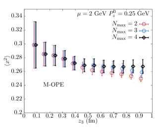
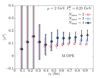
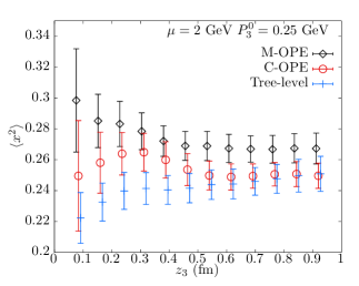
Figure 4: The top panel shows the $z_{3}$-dependence of $\langle x^{2}\rangle$ determined from the $\lambda=z_{3}P_{3}$ variation of ${\cal M}(z_{3}P_{3},z_{3}^{2},P_{3}^{0}=0.254{\rm GeV})$ at fixed values of $z_{3}$. The convergence with increasing the number $N_{\rm max}$ of even moments added to the NLO Mellin OPE (M-OPE) is shown. The middle panel shows a similar dependence for the determined $\langle x^{4}\rangle$. The bottom panel shows a comparison between the results of $\langle x^{2}\rangle$ that are determined from the NLO Mellin OPE and the conformal OPE. To display the effect of non-zero $\alpha_{s}$, we have shown the result using tree-level ($\alpha_{s}=0$) M-OPE.

We used the purely leading twist expression (i.e., we set the higher-twist correction $H$ and lattice correction $L$ to zero) in Eq. (9). By using the C-OPE for the leading-twist expression, we obtained the Gegenbauer moments $a_{n}$ by using them as the fit parameters. Similarly, by using M-OPE, we obtained the Mellin moments $\langle x^{n}\rangle$. Since each Mellin or Gegenbauer moment adds an additional fit parameter, we needed to truncate the OPE at a finite order $2N_{\rm max}$ which contains $N_{\rm max}$ number of even-$n$ moments; we successively increased $N_{\max}$ from 2 to 4. For C-OPE, the fits became unstable for $N_{\rm max}>3$ as the dependence on Gegenbauer moments beyond $a_{2}$ is rather weak. With M-OPE, we were able to go up to $N_{\rm max}=4$ in this analysis.

In the top panel of Fig. 4, we show $\langle x^{2}\rangle$ as a function of $z_{3}$ upto $z_{3}=0.91$ fm by applying M-OPE to ${\cal M}$ with $P_{3}^{0}=0.254$ GeV. We show the results using three different truncations $N_{\rm max}$. For $z_{3}<0.8$ fm, we can see that $N_{\rm max}=4$ is sufficient given the data precision. The near plateau in $\langle x^{2}\rangle$ around a value of about 0.28 shows that the leading-twist expansion describes the lattice data for ${\cal M}$ to a good approximation and that any higher-twist or lattice corrections are subdominant. This provides a validation of the leading-twist fixed-order perturbative framework that we are using to describe the nonpertubative lattice QCD data in the range of subfermi values of $z_{3}$ we use. The near plateau in $\langle x^{2}\rangle$ around a value of about 0.28 shows that our fitting form based on leading-twist perturbative expansion at NLO, with the choice of $\mu=2$ GeV, can describe the lattice data within the current statistical error. However, as shown in Refs. Ji et al. (2021b); Gao et al. (2022b), perturbation theory may become unreliable at large $z$ due to the resummation of large $\ln(z^{2}\mu^{2})$ Gao et al. (2021c), so a more dedicated study of the comparison between fixed-order and renormalization-group improved OPEs needs to be done to understand the results we have observed. Nevertheless, the central value of $\langle x^{2}\rangle$ changes by about 0.01 ($\approx 4\%$) as $z_{3}$ is increased from 0.1 fm to 0.6 fm. Hence, in the subsequent analysis of the data, we will include correction terms such as $H$ and $L$ to the leading-twist expansion. Since the correction itself is small, we were not able to deduce a possible functional form for the functions $H$ and $L$ that might be present, as we did in the case of the pion PDF in Ref Gao et al. (2020). In the middle panel of Fig. 4, we show a similar $z_{3}$ dependence of $\langle x^{4}\rangle$ at $\mu=2$ GeV. Since the analysis only made use of six different data points at each $z_{3}$, the errors on $\langle x^{4}\rangle$ are larger. Significant information on $\langle x^{4}\rangle$ enters ${\cal M}(\lambda,z^{2})$ only beyond $z_{3}>0.5$ fm, wherein we find initial indication that $\langle x^{4}\rangle\approx 0.15$, as we will find in the subsequent combined analysis of all the data. Within the larger errors, the data is consistent with $z_{3}$ independence.

In the bottom panel, we compare the values of $\langle x^{2}\rangle$ obtained using M-OPE (black squares) with that from C-OPE (red circles). For C-OPE, we converted the values of the fitted Gegenbauer moment $a_{2}$ to $\langle x^{2}\rangle$ through the simple linear relation (e.g., San Kim et al. (2012)), $\langle x^{2}\rangle=1/5+12/35a_{2}$. While results from both M-OPE and C-OPE are approximately $z_{3}$ independent, the values of $\langle x^{2}\rangle$ from M-OPE is about 3% higher than that from C-OPE. Since both M-OPE and C-OPE have converged well with respect to the OPE truncation, this is likely due to the remnant finite ${\cal O}(\alpha_{s})$ corrections that are missing from C-OPE, but captured correctly in M-OPE. We also show the result using $\alpha_{s}=0$ in the M-OPE, which we refer to as the tree-level result. Surprisingly, the tree-level result is also approximately plateaued, showing the effect of perturbative $\ln(\mu^{2}z_{3}^{2})$ in the OPE to be mild in the range of $z_{3}$ that we investigated using the choice of scale $\mu=2$ GeV. Henceforth, we will primarily show the results using M-OPE, and use C-OPE to compare those results with and serve as an indirect way to quantify the perturbative uncertainty by going from leading-log order to NLO.

VI.3 Determination of Mellin moments

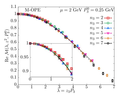
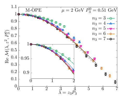
Figure 5: Fits of the leading-twist Mellin OPE to ${\cal M}(\lambda,z^{2},P_{3}^{0})$ using $\langle x^{2n}\rangle$ for $n\in[1,5]$ as fit parameters. The top and the bottom panels are for two-different fixed reference momenta $P_{3}^{0}=0.254$ GeV and 0.508 GeV used to form the ratio. The central values of the best fit curves from the Mellin OPE are compared with the lattice data; the solid curves are the results from using only the leading-twist OPE whereas the dashed curves are obtained by including a higher-twist term proportional to the conformal wave ${\cal F}^{(0)}_{0}(\lambda/2)$ along with $L(z_{3})$ lattice correction term. The data and the curves at different fixed momenta $P_{3}$ are distinguished by their colors.

Having shown the effectiveness of leading-twist OPE in capturing the $\lambda$ and $z_{3}^{2}$ dependencies of ${\cal M}(\lambda,z_{3}^{2})$, we now comfortably apply the framework to estimate the lowest two Mellin moments $\langle x^{2}\rangle$ and $\langle x^{4}\rangle$ through a combined fit to all the data for ${\cal M}(\lambda,z_{3}^{2})$ within a range of $z_{3}$. The fits are similar to the ones in the last section with the moments themselves as the free fit parameters. Therefore, the method is independent of any modeling of the $x$-dependence of the DA.

In the absence of any obvious visible evidence in Fig. 4 for lattice and higher-twist corrections, we simply modeled them. For the lattice correction that affects the lattice-like separations $z_{3}$, we assumed a possible presence of $(P_{3}a)^{2}$ corrections in the quasi-DA matrix element similar to the one in the quasi-PDF matrix element Gao et al. (2020). Thus, we chose a functional form,

$$L(z_{3},P_{3})=l_{2}(P_{3}a)^{2},$$ (42)

with $l_{2}$ being a real valued fit parameter in the modeled correction. In this way, such a term can effectively affect the leading twist terms at ${\cal O}(\lambda^{2})$ through a $z_{3}^{-2}$ type correction to the moments. In addition, there could be momentum independent ${\cal O}(a)$ or ${\cal O}(a^{2})$ corrections; since the continuum leading-twist expressions work quite well in describing the lattice data at a fixed lattice spacing, it is likely that such momentum independent corrections can be absorbed as part of the Mellin moments and the extracted DA themselves at that finite lattice spacing. For the higher-twist corrections, we followed a procedure similar to the one in Braun and Müller (2008), and assumed that the corrections resemble the one from twist-4 DA terms captured via a conformal OPE. For this, we added terms of the form,

$$H(z_{3},P_{3};N_{\rm HT})=\sum_{m=0}^{N_{\rm HT}-1}z_{3}^{2}h_{m}{\cal F}^{(0)}_{m}(\lambda/2),$$ (43)

with $h_{m}$ being the free parameters. In the above equation, we used the tree level conformal partial waves ${\cal F}^{(0)}_{m}$, obtained by setting $\alpha_{s}=0$ in Eq. (19), to avoid modeling the logarithmic $z_{3}^{2}$ dependencies using extra fit parameters. Since we introduce the corrections as a ratio via Eq. (11), the term $H$ can start at ${\cal O}((\lambda)^{0})$ as the condition that ${\cal M}^{\rm tw2,corr}(\lambda=\lambda^{0},z_{3})=1$ is satisfied by construction. Thus, we included ${\cal F}_{0}\sim(\lambda)^{0}$ as the leading term to Eq. (43). We used $N_{\rm HT}=0,1,2$ in order to keep the number of correction terms required to be small and at the same time take into account the sensitivity of the extracted results on the modeled higher-twist effects. However, one should note that there exists more complex approaches to model the functional form of $H$ (e.g., see Braun et al. (2004) that uses renormalon model) than the simpler functional parametrization that we adopt in this work.

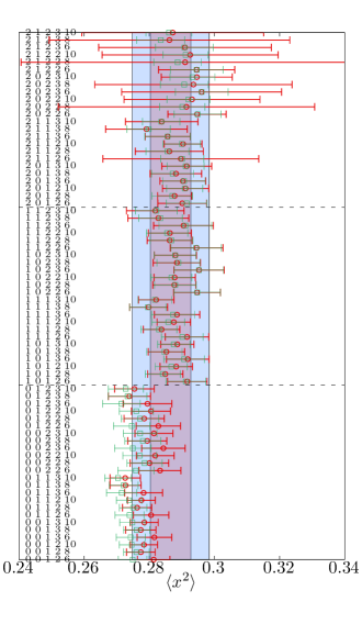
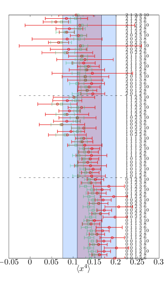
Figure 6: The scatter of best fit values of $\langle x^{2}\rangle$ and $\langle x^{4}\rangle$ from combined fits to $\lambda$ and $z^{2}$ dependencies of ${\cal M}(\lambda,z^{2},P_{3}^{0})$ over fit ranges $z_{3}\in[z_{3}^{\rm min},z_{3}^{\rm max}]$ and $P_{3}\in[P_{3}^{\rm min},P_{3}^{\rm max}]$. The red circles are obtained using Mellin moments as fit parameters without constraints, whereas the green circles are obtained using a positivity constraint on the pion DA. The variability comes from the number of higher-twist correction terms $N_{\rm HT}$, the number of lattice correction terms $N_{\rm LC}$, the reference momenta $n_{3}^{0}$ used in the ratio, and the ft ranges. The complete specification $(N_{\rm HT},N_{\rm LC},n_{3}^{0},z_{3}^{\rm min}/a,z_{3}^{\rm max}/a)$ is noted on the side of the points. The dashed lines separate cases with $N_{\rm HT}=0,1,2$ to see the overall effect of adding beyond leading-twist correction terms by hand. As determined from the unconstrained fits, the inner red band is the statistical error whereas the outer blue band includes both statistical and systematic errors. To compare, the values in the conformal limit are $\langle x^{2}\rangle=0.2$ and $\langle x^{4}\rangle=0.0857$.

In Fig. 5, we show the ratio ${\cal M}(\lambda,z_{3}^{2},P_{z}^{0})$ as a function of $\lambda=P_{3}z_{3}$, using only the lattice data with $z_{3}<0.91$ fm. The top and bottom panels are obtained using the reference momentum $P_{3}^{0}=0.254$ and 0.508 GeV respectively. We show the lattice data points from different $P_{3}>P_{3}^{0}$ together in the two plots, and we differentiate between them by the colors and symbols used. The insets in Fig. 5 simply magnify the range $\lambda<2$. We used the NLO Mellin OPE for the twist-2 contribution in Eq. (11), with and without the $H$ and $L$ correction terms that we discussed above to fit the lattice data for ${\cal M}$. Since the usage of non-zero $P_{3}^{0}$ is not common in the literature, we note that at a given fixed $\lambda$, the $z_{3}$ dependence comes from two sources even at leading-twist; namely, the $\ln(z_{3})$ dependence due to perturbative evolution and a polynomial dependence due to terms such as $P_{3}^{0}z_{3}$ in the denominator of the ratio. This is the reason that at $P_{3}^{0}=0.508$ GeV, one finds a somewhat larger $z_{3}$ dependence than one would expect only from the perturbative logarithm. To be clear, the presence of additional $P_{3}^{0}z_{3}$ type polynomial dependence on $z_{3}$ is not a disadvantage as such terms are captured within a leading-twist framework without any modelling, and the consequent spoiling of near universality with respect to $\lambda=z_{3}P_{3}$ is not a practical issue from the point of view of fits. We truncated the OPE using $N_{\rm max}=4$ number of even-$n$ moments. The dashed curves in Fig. 5 are the central values of the best fit curves when $N_{\rm HT}=1$ and $L(z_{3})$ terms are used as corrections, whereas the solid curves are obtained without any correction terms. In the example fit shown, we used a range $z_{3}\in[2a,0.608{\rm\ fm}]$. It is clear that the two types of fits work quite well in describing the lattice data. We found the fits with higher-twist correction terms to perform marginally better in terms of $\chi^{2}/{\rm df}$, and this shows up in the tendency for the dashed curves in Fig. 5 to pass closer to the central values of the lattice data points. Taking the case with $N_{\rm HT}=1$ and $P_{3}^{0}=0.25$ GeV shown in the top panel as a sample case to discuss the typical values of the fit parameters that we obtained in our fits, we find

$$\frac{h_{0}}{{\rm GeV}^{2}}=0.0067(29),\quad l_{2}=0.0008(11),$$ (44)

$$\langle x^{2}\rangle=0.2838(56),\quad\langle x^{4}\rangle=0.136(23),$$ (45)

$$\langle x^{6}\rangle=0.11(11),\quad\langle x^{8}\rangle=0.32(40),$$ (46)

$$\chi^{2}/{\rm df}=45.1/36$$ (47)

We see that our data sufficiently constrains only the lowest two even Mellin moments. The lattice correction term $l_{2}$ does not impact the fits, whereas the higher-twist correction term $h_{0}$ cannot be neglected. The value of $h_{0}=(81{\rm\ MeV})^{2}$ is in the ball-park of the value of higher-twist correction we empirically found in the quasi-PDF matrix element in Ref Gao et al. (2020). However, its value is small compared to the expectation for the twist-4 0-th Gegenbauer moment based on QCD sum rules Ball et al. (2006); Braun and Müller (2008), namely, $\delta^{2}_{\pi}\approx(300{\rm\ MeV})^{2}$.

Apart from the one case shown in Fig. 5, we also repeated the fits over the following 72 combinations of analysis choices: a) $N_{\rm HT}=0,1,2$, (b) with and without a lattice correction term, $N_{\rm LC}=0,1$, (c) $z_{3}^{\rm min}=2a,3a$ to take short-distance lattice artifacts into account, (d) $z_{3}^{\rm max}=0.456,0.608,0.76$ fm to take variations from higher-twist effects into account, (e) $P_{z}^{0}=0.254,0.508$ GeV for variation from reference momentum. In Fig. 6, we have shown the determination of $\langle x^{2}\rangle$ and $\langle x^{4}\rangle$ from each of the choices $(N_{\rm HT},N_{\rm LC},n_{3}^{0},z_{3}^{\rm min}/a,z_{3}^{\rm max}/a)$ as a data point (red circles). We specify the analysis choice to the side of each point. We found $\chi^{2}/{\rm df}<1.6$ for all the fits, and hence were acceptable. To make the trend in the fit parameters with respect to the added higher-twist terms visible, we have grouped the points in Fig. 6 in three sets with $N_{\rm HT}=0,1,2$ as indicated by the horizontal dashed lines. From the systematic shift in the determined values of moments, there appears to be a small but non-negligible effect of adding a $z_{3}^{2}{\cal F}^{(0)}_{0}(\lambda/2)$ term to the leading-twist OPE. The addition of one more term $z_{3}^{2}{\cal F}^{(0)}_{1}(\lambda/2)$ seems to only make the fits noisier. Thus, given the precision of the data, usage of $N_{\rm HT}=1$ seems to be sufficient. We show the scatter of the other fit parameters as well as the values of $\chi^{2}/{\rm df}$ in the various fits in Fig. 13 in Appendix B.

Using the analysis method we discussed earlier, we summarize the content of the red points in Fig. 5 as the following unweighted averages with the statistical and systematic errors:

$$\langle x^{2}\rangle = 0.2866(62)(56),$$ (48)

$$\langle x^{4}\rangle = 0.138(28)(34),$$ (49)

at a scale $\mu=2$ GeV. These summary estimates are shown in the vertical bands of Fig. 5; the inner band includes the statistical error only, whereas the outer one includes both the statistical and systematic error. It can be seen that the outer band covers most of the scatter due to the various choices, and hence is representative of our data.

If we assume that the pion DA is positive at all $x$ at $\mu=2$ GeV, then we can improve the stability of fits by imposing inequalities on the Mellin moments that follows from $\phi(x,\mu)>0$, and subsequent derivatives of $\langle x^{n}\rangle$ with respect to $n$ at values infinitesimally closer to integer values. Namely, as we explain in Gao et al. (2020), we obtain the inequalities (a) $\langle x^{n}\rangle>\langle x^{n+2}\rangle$ and (b) $\langle x^{n+2}\rangle+\langle x^{n-2}\rangle>2\langle x^{n}\rangle$. In the analysis, we imposed the two constraints through a change of variables $\langle x^{2n}\rangle\equiv\sum_{i=n}^{N_{\rm max}}\sum_{j=i}^{N_{\rm max}}e^{-\lambda_{j}}$. We have shown the results of such constrained fits as the green circles in the two panels in Fig. 5. We find the resulting values of the two lowest moments to be well determined, especially as the number of fit parameters is increased when we set $N_{\rm HT}=2$. In the case of $\langle x^{4}\rangle$, such a procedure results in more precise estimates compared to the unconstrained estimates shown as red circles. We find from this constrained analysis that

$$\langle x^{2}\rangle = 0.2848(52)(71),$$ (50)

$$\langle x^{4}\rangle = 0.124(11)(20).$$ (51)

at $\mu=2$ GeV.

Using the model-independent estimates of the Mellin moments themselves, we can reach a few conclusions. The values of these two Mellin moments in the large $Q^{2}$ limit of DA, $\phi(x)=4(1-x^{2})/3$, are $\langle x^{2}\rangle=0.2$ and $\langle x^{4}\rangle=0.0857$. These differ quite significantly from the values we determined, and hence we can conclude that the pion DA at the physical point and at a scale of $\mu=2$ GeV differs from the asymptotic DA. In fact, since $\langle x^{2}\rangle>0.2$, we can expect the $x$-dependent DA to be flatter compared to the asymptotic DA. The DA cannot be a completely flat DA Radyushkin (2009), $\phi(x)=1/2$ which is characterized by $\langle x^{2}\rangle=1/3\approx 0.33$, and $\langle x^{4}\rangle=0.2$. We can consider another extreme case of a double humped Chernyak-Zhitnitsky (CZ) DA Chernyak and Zhitnitsky (1982), $\phi(x)=15(1-x^{2})x^{2}/4$, at $\mu=2$ GeV, with Mellin moments as $\langle x^{2}\rangle=0.4285$ and $\langle x^{4}\rangle=0.2381$. These values are not compatible with the values we find. Instead, if we assume a simple one-parameter ansatz, $\phi(x)={\cal N}(1-x^{2})^{\alpha}$, and solve for $\alpha$ using the value of $\langle x^{2}\rangle=0.2866$, we find the exponent should be around $\alpha=0.244$. In the next subsection, we perform more elaborate fits to such Ansätze.

We performed a similar set of analyses using the C-OPE for the leading-twist contribution in Eq. (11). However, we were not able to obtain stable fits with a more complex $N_{\rm HT}=2$ correction term to C-OPE without imposing any constraints on the Gegenbauer moments, which resulted in a spurious negative-valued $a_{2}$ at the cost of a large-valued higher-twist coefficient $h_{1}$. Since it is likely due to overfitting of the data, we excluded this analysis choice. To summarize, using all other combinations of analysis choices, we found $a_{2}=0.227(18)(23)$ and $a_{4}=-0.16(13)(30)$. These values correspond to Mellin moments, $\langle x^{2}\rangle=0.2779(63)(79)$ and $\langle x^{4}\rangle=0.121(15)(28)$, using the linear relations between $a_{n}$ and $\langle x^{n}\rangle$ (e.g., San Kim et al. (2012)). It is reassuring that two ways of incorporating the leading-twist OPE result in similar values of the first two Mellin moments. It is also clear that when written using C-OPE, the essential non-vanishing contribution mainly comes from the $a_{2}$ Gegenbauer moment. The non-vanishing value of $\langle x^{4}\rangle$ we find using the Mellin OPE, while being non-trivial information from the perspective of M-OPE, becomes trivial when expressed in terms of non-vanishing $a_{2}$ and a vanishing $a_{4}$ from the C-OPE perspective.

As a way of estimating perturbative uncertainty, we performed the above set of analyses at scales of $\mu=4$ GeV and $\sqrt{2}$ GeV, using $\alpha_{s}(4{\rm\ GeV})=0.227$ and $\alpha_{s}(\sqrt{2}{\rm\ GeV})=0.3607$. We then perturbatively ran the estimated Mellin moments to the fixed scale $\mu=2$ GeV using the NLO implementation that incorporates the mixing among the Mellin moments (as discussed in Ref. Agaev et al. (2011)). Through this procedure, we found $\left[\langle x^{2}\rangle,\langle x^{4}\rangle\right]$ at $\mu=2$ GeV to be $\left[0.2822(85)(47),0.126(30)(35)\right]$ and $\left[0.2928(57)(76),0.148(20)(34)\right]$ through evolution from $\mu=4$ GeV and $\sqrt{2}$ GeV respectively. These values agree with the estimates from the analysis performed exactly at $\mu=2$ GeV within the statistical and systematical errors. Thus, we expect the perturbative uncertainties to be less important compared to the combined statistical and systematical errors.

Finally we compare our findings for the Mellin moments with some recent lattice QCD calculations at $\mu=2$ GeV. The work Arthur et al. (2011) using a dynamical QCD simulation and using the local twist-2 operator approach obtain $\langle x^{2}\rangle=0.28(1)(2)$. Another series of works from RQCD that culminated in Ref Bali et al. (2019) using the local operator approach obtain $\langle x^{2}\rangle=0.240(6)(2)(3)(2)$ at the physical point and take into account various kinds of systematical errors. Whereas, the usage of the leading-twist expansion method using current-current correlators Bali et al. (2018b) results in a scatter of values around $\langle x^{2}\rangle\approx 0.3$. Using the quasi-DA matrix element as used in this work, but using LaMET $x$-space matching, the work Zhang et al. (2020) estimates $\langle x^{2}\rangle=0.244(30)(20)$, and the most recent work Hua et al. (2022) using the hybrid-renormalization method Ji et al. (2021b) estimates $\langle x^{2}\rangle=0.300(41)$. Our result lies in the ball park value of previous estimates, but it is about 2.4-$\sigma$ (including statistical and systematic errors in both works naively as the net error) larger from the estimate using the local operator approach in Ref Bali et al. (2019). In the future, we need to investigate the remaining systematical uncertainties in our work that we did not quantify, such as the effect of finite lattice spacing, and see if the tension between the values of Mellin moments obtained with two completely different methods, reduces or persists.

VI.4 Prior-sensitive reconstruction of the pion DA

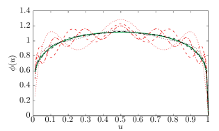
Figure 7: The convergence of an example DA, $\phi(x)=1.47x^{0.2}(1-x)^{0.2}$, shown as the green curve, when expanded in $C_{2n}^{3/2}$, shown as the red curves, and in another basis $C_{2n}^{0.9}$, shown as the black curves. The truncation of the expansions in $n$ upto $2,4,6$ are shown as dotted, dashed and dot-dashed curves respectively. The expansion in $C_{2n}^{1/2+\alpha}$ with $\alpha=0.4$ which is close to the actual exponent, 0.2, converges much faster than with $C_{2n}^{3/2}$.

Our determination of the lowest two Mellin moments in a model-independent manner is the important result in this paper. However, within the framework of fitting phenomenology motivated Ansätze to the lattice data, we can reconstruct the $x$-dependence of the DA, $\phi(x)$. For convenience, we define the variable $u$ via

$$x=2u-1,$$ (52)

so that the DA has support from $0$ to $1$. In principle, once we know all the Gegenbauer moments from fits to C-OPE, or inferred from M-OPE, we can perform a model-independent reconstruction using

$$\phi(u)=6u(1-u)\sum_{n=0}a_{2n}C_{2n}^{3/2}(1-2u).$$ (53)

The caveat that all the moments $a_{2n}$ need to be known makes such an approach not usable in practice; as we saw, the real-space quantity ${\cal M}(\lambda,z^{2})$ converges in the accessible range of $\lambda<6$ rapidly with respect to the number of Gegenbauer moments $a_{n}$ (as the main content of ${\cal M}$ can be summarized approximately with a value of $a_{2}$), whereas the corresponding convergence in $u$ (or $x$)-space is rather slow. The problem is easy to understand by considering a behavior $\phi(u)={\cal N}u^{\alpha}(1-u)^{\alpha}$. In the last section, from the value of $\langle x^{2}\rangle$, we expected $\alpha\approx 0.25$, which differs significantly from the leading term with $\alpha=1$ in Eq. (53).

We can improve the convergence by using a complete basis that is orthonormal with respect to a weight function, $w(u)=u^{\alpha}(1-u)^{\alpha}$, rather than the weight function $w(u)=u(1-u)$ that the Gegenbauer polynomials $C_{n}^{3/2}$ are orthonormal with respect to. Such an idea was pursued in Chang et al. (2013a) using the Gegenbauer polynomial basis $C_{n}^{\alpha+1/2}(1-2u)$, which we follow in this paper. To impose the evenness of $\phi(u)$ around $u=1/2$, we restrict the functions to even $n$. That is, we expand,

$$\phi(u)={\cal N}u^{\alpha}(1-u)^{\alpha}\sum_{n=0}^{N_{G}+1}s_{n}C_{2n}^{\frac{1}{2}+\alpha}(1-2u),$$ (54)

with $s_{0}=1$. The value of $\alpha$ describing the family of complete functions is arbitrary, but a usage of $\alpha$ that is close enough to the large/small-$x$ exponent leads to a better convergence with respect to the truncation order $N_{G}$. In Fig. 7, we show a specific example of the better convergence of an example DA, $\phi(u)=1.47u^{0.2}(1-u)^{0.2}$, when expanded in a nearby $C_{n}^{0.9}$ polynomial basis as compared to an expansion in $C_{n}^{3/2}$ polynomials. We note that the polynomials $C_{n}^{\alpha+1/2}(1-2u)$ are proportional to another complete basis, the Jacobi polynomials, $P_{n}^{\alpha,\beta}(1-2u)$ for $\alpha=\beta$, that have been proposed Karpie et al. (2021) as a good choice in the analysis of PDFs even when $\alpha\neq\beta$.

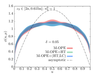
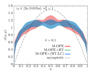
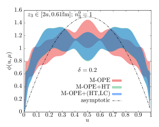
Figure 8: The reconstructed $u=2x-1$ dependent pion distribution amplitude $\phi(u,\mu)$ at $\mu=2$ GeV using the $C_{2n}^{\alpha+1/2}$ basis from $n=1$ to $n=N_{G}=4$. For all the cases shown, the fit range is $z_{3}\in[2a,0.61{\rm fm}]$, and $P_{3}^{0}=0.254$ GeV. The top, middle and bottom panels are obtained using prior widths $\delta=0.05$, 0.1 and 0.2 on the coefficients of $C_{n}^{\alpha+1/2}$ respectively. The choices of $\alpha$ determining the Gegenbauer polynomial family were obtained from a one-parameter fit as explained in the text.

First, we determined the best fit values of the exponent $\alpha$ of the one-parameter Ansatz,

$$\phi_{\rm 1-param}(u)={\cal N}u^{\alpha}(1-u)^{\alpha},$$ (55)

that best describes the lattice data via Eq. (11) for each analysis choice that we described earlier. Essentially, the parameter $\alpha$ enters the fits through the $\alpha$-dependent Mellin moments. Therefore, unlike the model-independent analysis of moments that we presented in the previous subsection, all the moments are now related through a single unknown parameter $\alpha$. We truncated the Mellin OPE at order $N_{\rm max}=6$ as before. For different analysis choices, we found the values of the $\alpha$ to lie in a range between $0.2$ to $0.32$.

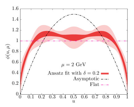
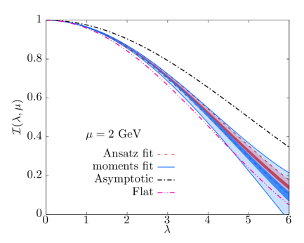
Figure 9: (Top panel) The pion DA reconstructed using the $C_{n}^{1/2+\alpha}$ basis with the constraint $\delta=0.2$. The inner dark band is the statistical error band. The outer light band is the combined statistical and systematic error band. Variations in the fitted range of $z_{3}$, reference momentum $P_{z}^{0}$, type of lattice correction and higher-twist corrections added were taken into account in summarizing the result in the figure. The asymptotic limit of DA is shown as the black curve. (Bottom panel) The plot shows the light-front ${\overline{\mathrm{MS}}}$ pion ITD corresponding to the pion DA in the panel above, as the red band. The ITD expected from the fits to Mellin moments is shown as the blue band. In both cases, statistical and combined statistical-systematical error bands are shown. For comparison, the ITDs corresponding to the asymptotic DA (black dot-dashed curve) and flat DA (magenta dot-dashed curve) are also shown.

In the next step, we generalized the parametrization for the DA by an expansion in $C_{n}^{1/2+\alpha}$ as given in Eq. (54). We followed the approach in Ref Egerer et al. (2022) to slowly generalize from the one-parameter Ansatz above to more flexible ones using a complete basis of functions to capture the corrections to Eq. (55). We used the best fit values of $\alpha$ from the one-parameter fits from the previous step to choose the basis, $C_{n}^{1/2+\alpha}$. Even though the values of $\alpha$ did not change much based on the analysis choices, we took care of using the corresponding $\alpha$ values for a given analysis choice. The fit parameters are the coefficients $s_{n}$ in Eq. (54), which enter via the Mellin moments or Gegenbauer moments (the implementation of fits can be made computationally faster by pre-evaluating the moments of Gegenbauer Polynomials $\int_{0}^{1}(2u-1)^{n}u^{\alpha}(1-u)^{\alpha}C^{1/2+\alpha}_{n}du$, from which the Mellin moments are obtained as linear combinations.) We imposed the external constraint on the allowed amount of fluctuations about $\phi_{\rm 1-param}$ through constraints on the expansion coefficients that $|s_{n}|\lesssim\delta$. We realized this via Gaussian priors on $s_{n}$ added to the $\chi^{2}$ using the central values and widths of the priors of all $s_{n}$ being $0$ and $\delta$ respectively. One should however note that there is a priori no expected value for $\delta$ simply from general considerations. From practical considerations, we will present the reconstructions by imposing successively weaker constraints from $\delta=0.05$ to $\delta=0.2$. For even larger values of $\delta$, we found the reconstruction to be very noisy and oscillatory.

In the panels of Fig. 8, we show the reconstructions of DA at $\mu=2$ GeV using prior widths $\delta=0.05,0.1$ and 0.2 from top to bottom respectively. For the cases we show, we performed the fits over a range $z_{3}\in[2a,0.61{\rm\ fm}]$ and using a reference momentum $P_{3}^{0}=0.254$ GeV. In each panel, we show the reconstructions based on M-OPE without any correction terms, with $N_{\rm HT}=1$, and with $(N_{\rm HT},N_{\rm LC})=(1,1)$. The changes due to such variations are small, especially the effect of $N_{\rm LC}$ being negligible. From $\delta=0.05$ to 0.1, the effect of relaxing the prior of $s_{n}$ is primarily to increase the statistical error on the bands while closely agreeing with the one-parameter reconstruction. The reconstructed DA starts becoming slightly oscillatory and with larger error band when $\delta$ is relaxed to 0.2. Unlike the case of PDFs, which typically show a subdued prior and model dependence, we found the reconstructed DA to be sensitive to the prior that is applied. This is not surprising given that the essential content in our quasi-DA matrix element in the range of $\lambda$ we used is $a_{2}$, and the problem posed by such limited information in the DA reconstruction is well known in the literature. However, the use of the $C_{n}^{1/2+\alpha}$ basis was useful to quantitatively and systematically reconstruct the pion DA that depends on the extent to which one allows the DA to deviate from the default one-parameter model. Thus, the panels of Fig. 8 together convey this prior dependent knowledge of DA from our quasi-DA matrix element.

We repeated the above fits for all analysis choices, which now includes the truncation order $N_{G}=2,3$ and 4 in Eq. (54). In the top panel of Fig. 9, we show our estimate of the pion DA as a function of $u$, after taking into account all the analysis variations, and summarize them with the statistical and systematic error bands. To be cautious, we present the reconstruction using a relatively broad prior width $\delta=0.2$ on the expansion coefficients. Nevertheless, the reconstruction in the case of DA is sensitive to the value of $\delta$, however large it is, and hence, one should interpret the reconstruction of DA in Fig. 9 as a specific $u$-dependence, given a somewhat broad prior. We compare our result with the asymptotic DA shown as the black dashed curve. Within the precision allowed at $\delta=0.2$, we can only resolve an overall flat DA over a range of $u\in[0.2,0.8]$ with sharp fall offs, $u^{\alpha}$ and $(1-u)^{\alpha}$ with $\alpha\approx 0.3$, to 0 on either side. If one focuses only on the central value of the reconstructed DA, one sees a tendency for a platykurtic DA as noted in Refs Stefanis (2014); Stefanis and Pimikov (2016); Stefanis (2020). The lattice data does not have the sensitivity to further resolve the concavity or convexity within the flatter regions, unless one is willing to impose a more stringent prior width $\delta$. Apart from providing a reconstruction of the DA, the ansatz based analysis also provides a way to estimate the moments of DA. The usage of ansatz can be thought of as a way to regulate the values of moments at larger-$n$ for which the lattice data is less constraining, and therefore, provides robust values for smaller-$n$ moments. From the Ansatz based analysis above with $\delta=0.2$, we estimate the Mellin moments as

$$\langle x^{2}\rangle = 0.2845(44)(58),$$ (56)

$$\langle x^{4}\rangle = 0.1497(50)(38).$$ (57)

By comparing the values with Eq. (49), we see that the ansatz based reconstruction for $\langle x^{2}\rangle$ agrees quite well with the completely model-independent reconstruction. The estimates of $\langle x^{4}\rangle$ also agree with each other, however, the usage of ansatz has substantially reduced the error. Thus, from both the model-independent moments analysis and the model-dependent reconstruction analysis, we find the values of $\langle x^{2}\rangle$ and $\langle x^{4}\rangle$ to be the quantities that we could reliably extract from our lattice data.

As another way to summarize our results with less modeling artifacts, we present the ${\overline{\mathrm{MS}}}$ light-front ITD corresponding to the pion DA in the bottom panel of Fig. 9 in the range of $\lambda$ that we have lattice data for and performed our analysis on. To infer the ${\overline{\mathrm{MS}}}$ ITD, we used Eq. (12). Since we need only the information on the Mellin moments to construct the light-front ITD, we show the resultant ITD based on the above Ansatz-based analysis as the red band enclosed between the dot-dashed lines, and the result based on the Mellin moments analysis in the previous subsection as the blue band enclosed between solid lines. In both cases, the darker inner bands are the statistical error bands whereas the lighter outer bands include both statistical and systematical errors. We see that both the model-independent and ansatz-dependent reconstructions have similar behavior in the range of $\lambda$ that is constrained by the lattice data, with the latter being a more precise determination. We show the light-front ITD corresponding the asymptotic DA as the black dot-dashed curve. We also compare our result with the expected ITD for a flat pion DA shown as the magenta dot-dashed curve. Our result is clearly below the asymptotic DA expectation, and closer to the expectation from a flatter DA. This expectation is a less model-dependent manifestation of the DA reconstruction seen in the top panel.

VI.5 Relation between form factors and DA at high momentum transfer from perturbative factorization

The key quantities that characterize exclusive QCD processes, such as such as the photon-pion transition form factor Behrend et al. (1991); Gronberg et al. (1998); Aubert et al. (2009); Uehara et al. (2012), electromagnetic form factors and GPDs can be factorized into convolutions of DAs and the perturbatively-calculable partonic hard-scattering amplitudes if the momentum transfer is sufficiently large. For electromagnetic form factor this factorization was introduced long time ago Efremov and Radyushkin (1980); Farrar and Jackson (1979); Lepage and Brodsky (1980). For photon-pion transition it was discussed in Refs. Melic et al. (2003); Gao et al. (2022a), and for gravitational form factors it was discussed in Refs.  Tong et al. (2021, 2022), while for GPDs it was discussed in Refs. Hoodbhoy et al. (2004); Sun et al. (2022). The energy scale where this leading-twist DA-based factorization may work is unknown at present. This an important question that can only be answered by experiments or through lattice QCD computations. In this subsection, we put aside this question and simply make predictions for electromagnetic and gravitational form factors of the pion based on leading twist factorization and our DA results. These predictions can be compared to the lattice or experimental results at large momentum transfer and clarify the range of applicability of the leading twist factorization for the form-factors.

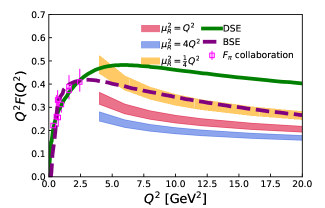
Figure 10: The pion electromagnetic form factors reconstructed from DA using LO matching and evolution are shown; the different bands capture the variation from using factor 2 variation in scale $\mu_{R}$ used to determine $\alpha_{s}$. The experimental data from $F_{\pi}$ collaboration Huber et al. (2008) as well as the calculations from Dyson-Schwinger equation (DSE) Chang et al. (2013b) and Minkowski-space Bethe-Salpeter equation (BSE) Ydrefors et al. (2021) are shown.

At large $Q^{2}$, the pion electromagnetic form factors $F_{\pi}(Q^{2})$ can be factorized as

$$F_{\pi}(Q^{2}) =\int^{1}_{0}\int^{1}_{0}dxdy\ \Phi^{*}(v,\mu^{2}_{F})$$ (59)

$$\qquad\times T_{F}(u,v,Q^{2},\mu^{2}_{R},\mu^{2}_{F})\Phi(u,\mu^{2}_{F})\,,$$

where $Q^{2}$ is the momentum transfer and $T_{F}$ is the hard-process kernel. Though the form factor $F_{\pi}(Q^{2})$ is scale independent, the fixed-order perturbative factorization introduces dependence on both renormalization and factorization scales $\mu^{2}_{R}$ and $\mu^{2}_{F}$. Here $\Phi(u,\mu^{2}_{F})$ is defined as,

$$\Phi(u,\mu^{2}_{F})=\frac{f_{\pi}}{2\sqrt{2N_{c}}}\phi(u,\mu^{2}_{F}),$$ (60)

where $f_{\pi}$ is the pion decay constant discussed in Section V.1. At leading order (LO), the hard kernel reads Melic et al. (1999),

$$T_{F}^{(0)}(u,v,Q^{2})=\alpha_{s}(\mu^{2}_{R})\frac{4}{3}\frac{16\pi}{Q^{2}\bar{u}\bar{v}},$$ (61)

with $\bar{u}=1-u$ and the running coupling constant

$$\alpha_{s}(\mu^{2}_{R})=\frac{4\pi}{\beta_{0}\ln(\mu^{2}_{R}/\Lambda^{2}_{\rm QCD})}\,,$$ (62)

where $\beta_{0}=11-\frac{2}{3}n_{f}$, and we use $n_{f}=3,\Lambda_{\rm QCD}=0.2$ GeV in this paper. We take our model fit result at the initial scale $\mu_{0}$ = 2 GeV, and evolved it to $\mu_{F}$ by first expanding $\phi(u,\mu_{0})$ in the Gegenbauer basis in Eq. (53) up to a sufficiently large order $n=n_{\rm max}=20$, and then evolving those Gegenbauer moments from $a_{n}(\mu_{0})$ to $a_{n}(\mu_{F})$ using

$$a_{n}(\mu_{F}) =\left(\frac{\alpha_{s}(\mu^{2}_{F})}{\alpha_{s}(\mu^{2}_{0})}\right)^{\gamma_{n}^{(0)}/\beta_{0}}a_{n}(\mu_{0})\,.$$ (63)

We choose $\mu_{R}=\mu_{F}=Q$ as the central value of the scale setup, and vary the renormalization scale $\mu_{R}$ by a factor of 2 to estimate the perturbation uncertainty. For the ease of implementation, we used the 1-parameter Ansätze $\phi_{\rm 1-param}(x,\mu_{R})$ from our analysis using $(N_{\rm HT},N_{\rm LC},n_{3}^{0},z_{3}^{\rm min},z_{3}^{\rm max})=(1,1,1,2a,8a)$.

The results are shown in Fig. 10 with statistical error bands and compared with the experimental data from the $F_{\pi}$ collaboration Huber et al. (2008) as well as the calculations from the Dyson-Schwinger equation (DSE) Chang et al. (2013b) and Minkowski-space Bethe-Salpeter equation (BSE) Ydrefors et al. (2021). As one can see, our prediction using the LO kernel is systematically lower than the DSE and BSE calculations. It was found that the matched form factors could increase with NLO corrections Melic et al. (1999), and the higher-twist corrections may also make a significant contribution Raha and Kohyama (2010). However, all these arguments can only be tested by the future experimental results with large momentum transfer $Q^{2}$ up to 6 $\rm GeV^{2}$ of the JLAB E12-09-001 experiment Dudek et al. (2012) and up to 40 $\rm GeV^{2}$ of the new Electron-Ion Collider (EIC) facility Arrington et al. (2021).

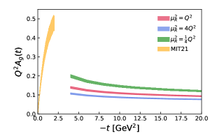
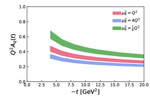
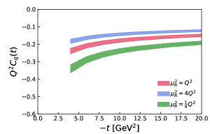
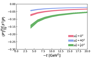
Figure 11: The gluon GFFs $Q^{2}A_{g}(t)$, quark GFFs $Q^{2}A_{q}(t)$ and $Q^{2}C_{q}(t)$ as well as the pion trace anomaly $\langle P^{\prime}|\frac{\beta(g)}{2g}F^{2}|P\rangle$ at large $-t$ predicted by our determination of pion DA are shown. The bands come from the statistic errors and we vary the renormalization scale $\mu_{R}$ by a factor of 2 to estimate the perturbation uncertainty. The direct lattice calculation of pion gluon GFF $A_{g}(-t)$ Pefkou et al. (2022) (the multipole fit result) using unphysical pion mass $m_{\pi}=$ 450 MeV is shown (MIT21, the yellow band in the top-left panel) for comparison.

The gravitational form factors (GFFs) of the pion are the transition matrix elements of the QCD energy momentum tensor,

$$T^{\mu\nu}_{\rm QCD}=T^{\mu\nu}_{q}+T^{\mu\nu}_{g}.$$ (64)

Though $T^{\mu\nu}_{\rm QCD}$ is conserved, and is therefore UV finite and scale independent, the quark and gluon contributions, $T^{\mu\nu}_{q}$ and $T^{\mu\nu}_{g}$, are not and depend on the renormalization scale $\mu_{R}$. This dependence is governed by the corresponding anomalous dimension. The gluon gravitational form factors for the pion can be parametrized as,

$$\langle P^{\prime}|T^{\mu\nu}_{g}(\mu_{R})|P\rangle=2\bar{P}^{\mu}\bar{P}^{\nu}A^{\pi}_{g}(t,\mu_{R})$$ (65)

$$\qquad+\frac{1}{2}(\Delta^{\mu}\Delta^{\nu}-g^{\mu\nu}\Delta^{2})C^{\pi}_{g}(t,\mu_{R})+2m^{2}g^{\mu\nu}\overline{C}^{\pi}_{g}(t,\mu_{R})\,,$$

where $\bar{P}=(P^{\prime}+P)/2$ is the average momentum, $\Delta=P^{\prime}-P$ is the momentum transfer, and $-t=-\Delta^{2}=Q^{2}$. Similar to the case of the electromagnetic form factor, the leading-twist GFFs perturbative factorization reads,

$$A^{\pi}_{g}(t,\mu_{R}) =\int dudv\ \Phi^{*}(v,\mu_{F})$$

$$\qquad\times\mathcal{A}^{\pi}_{g}(u,v,t,\mu_{R},\mu_{F})\Phi(u,\mu_{F})\,,$$ (66)

where $\mu_{F}$-dependence can be introduced in $A^{\pi}_{g}$ due to the use of a fixed-order hard kernel. At leading order, the kernels are Tong et al. (2021),

$$\mathcal{A}^{\pi}_{g}(u,v,t,\mu_{R},\mu_{F}) =\mathcal{C}^{\pi}_{g}(u,v,t,\mu_{R},\mu_{F})$$

$$=\frac{8\pi\alpha_{s}(\mu_{R})C_{F}}{-t}(\frac{1}{u\bar{u}}+\frac{1}{v\bar{v}})\,.$$ (67)

Due to the traceless feature of Eq. (65) one also has the relation $\overline{\mathcal{C}}^{\pi}_{g}=-\mathcal{C}^{\pi}_{u+d}=\frac{t}{4m^{2}}\mathcal{C}^{\pi}_{g}$. In terms of the same factorization formula, the hard coefficients $\mathcal{A}_{q}$ and $\mathcal{C}_{q}$ in the quark sector are,

$$\mathcal{A}^{\pi}_{q}(u,v,t,\mu_{R},\mu_{F}) =\frac{8\pi\alpha_{s}(\mu_{R})C_{F}}{-t}\frac{u+v+1}{\bar{u}\bar{v}},$$ (68)

$$\mathcal{C}^{\pi}_{q}(u,v,t,\mu_{R},\mu_{F}) =\frac{8\pi\alpha_{s}(\mu_{R})C_{F}}{-t}\frac{u+v-3}{\bar{u}\bar{v}}.$$ (69)

In addition, the gluon scalar FF defined as,

$$\langle P^{\prime}|F^{a,\mu\nu}F^{a}_{\mu\nu}|P\rangle=m^{2}_{\pi}G_{\pi}(t,\mu_{R}),$$ (70)

is closely related to the trace anomaly Ji (1995),

$$T_{\mu}^{\mu}=\frac{\beta(g_{s})}{2g_{s}}F^{a,\mu\nu}F^{a}_{\mu\nu}.$$ (71)

Using the same factorization convention as Eq. (VI.5), the leading-order hard kernel reads Tong et al. (2022),

$$\mathcal{G}^{\pi}_{q}(u,v,t,\mu_{R},\mu_{F})=\frac{16\pi\alpha_{s}(\mu_{R})C_{F}}{m_{\pi}^{2}}(\frac{1}{u\bar{v}}+\frac{1}{\bar{u}v}).$$ (72)

Comparing to the tensor GFFs $A_{q,g}$ and $C_{q,g}$ shown above, one can observe that $\mathcal{G}^{\pi}_{q}$ does not have a $1/(-t)$ pre-factor and therefore will become flat for large $-t$. In Fig. 11, we show the perturbatively determined GFFs and pion trace anomaly at large $-t$ as expected from our determination of pion DA. The bands come from the statistical errors and we vary the renormalization scale $\mu_{R}$ by a factor of 2 to estimate the perturbation uncertainty. The direct lattice calculation of the pion gluon GFF $A_{g}(-t)$ Pefkou et al. (2022) (the multipole fit result) using unphysical pion mass $m_{\pi}=$ 450 MeV is shown (MIT21, the yellow band in the top-left panel) for comparison. And it can be seen our estimate of the perturbative contribution is much smaller, which could come from sizable higher-order perturbative or higher-twist contribution. Direct lattice calculations or experimental results at large $-t$ are needed to clarify the issue.

In order to perform the above perturbative convolutions, we relied on the Ansatz-based reconstruction to a large extent. Instead, one could ask if there is a way to perform an alternate less model dependent analysis based only on the ITD in the range of $\lambda$ spanned by the lattice data, or equivalently, only using the moments that the lattice data is sensitive to. To address this question, we can refer to the LO perturbative convolution in Eq. (59) for electromagnetic form-factor that makes use of the integral,

$$\langle(1-u)^{-1}\rangle=\langle u^{-1}\rangle=\int_{0}^{1}du\frac{\phi(u,\mu)}{u}.$$ (73)

Using Eq. (53), one can see that, $\langle u^{-1}\rangle=3\sum_{n=0}^{\infty}a_{2n}(\mu)$. If one truncates the sum over Gegenbauer moments up to $n=1$ at $\mu=2$ GeV, then one finds $\langle u^{-1}\rangle=3.72(45)$, whereas when one sums over 20 Gegenbauer moments using the 1-parameter Ansätze, we get $\langle u^{-1}\rangle=4.87(19)$. As an alternative, we can write Eq. (73) using only the ITD as,

$$\langle u^{-1}\rangle=\lim_{\lambda_{\rm max}\to\infty}\int_{0}^{\rm\lambda_{\rm max}}{\cal I}(\lambda,\mu)\sin\left(\frac{\lambda}{2}\right)d\lambda.$$ (74)

With $\lambda_{\rm max}\approx 6$ as in this work (see bottom panel of Fig. 9), we find this region of ${\cal I}(\lambda,\mu)$ to contribute 2.64(2) to $\langle u^{-1}\rangle$, which is only about 50% to the Ansatz-based expectation for $\langle u^{-1}\rangle$, and the rest comes from $\lambda>\lambda_{\rm max}$. Therefore, for the two model-independent methods to be reliable, one has to truncate at much higher Gegenbauer moments or larger $\lambda$, which poses a challenge for lattice calculations. As a result, one has to rely on the Ansätze for the $x$-dependence of DA, but the systematic uncertainty from truncation is transformed to the model dependence of the Ansätze. It would be important in the future to compare and cross-check our current results for the form factors here with the expectations based on $x$-space LaMET DA matching on the same ensemble.

VII Conclusions

We presented a lattice QCD study of the quasi-DA matrix element in real-space using the leading-twist OPE method for the first time. We performed our study at the physical point using clover-improved Wilson valence quark propagators determined on a physical HISQ ensemble. The quantities central to this work are the renormalization group invariant ratios of quasi-DA matrix elements, with non-zero momenta in both the numerator and denominator; the non-zero momenta were inevitable as well as helped us remain closer to the leading-twist approximation. In the first part of the paper, we adapted the results from Refs. Radyushkin (2019); Braun and Müller (2008) and presented the analytical perturbative results for the leading-twist expansion in the forms of the Mellin OPE at next-to-leading order and the conformal OPE at leading-log order. These expressions formed the basis for our determination of the pion DA from quasi-DA matrix elements.

From the leading-twist description of $z\cdot P$ and $z^{2}$ dependencies of the ratios of quasi-DA matrix elements, we extracted the Mellin moments and captured the $x$-dependence of the pion DA based on fits to various Ansätze. We first checked the validity of leading-twist dominance in our matrix element using a fixed-$z^{2}$ analysis. Then, from a model-independent determination via fits to the few lowest Mellin moments at a factorization scale $\mu=2$ GeV, we were able to obtain a relatively precise determination of the second Mellin moment, $\langle x^{2}\rangle=0.287(6)(6)$, and for the fourth Mellin moment, we obtained $\langle x^{4}\rangle=0.14(3)(3)$; the first parenthesis gives the statistical error and the second one specifies the systematical error coming from variations in various analysis choices, such as fit ranges for $z^{2}$. Based on NLO perturbative evolution of our corresponding results at different $\mu$ evolved to $\mu=2$ GeV, we estimated our perturbative uncertainty to be within our combined statistical and systematical errors. We reached a similar conclusion from the differences in the estimates of the Mellin moments from the Mellin-OPE and Conformal-OPE. We found the Ansatz based reconstruction of the $x$-dependence of the pion DA to be sensitive to the model used; by using a complete set of functions to expand the DA and by imposing constraints on their expansion coefficients, we systematically reconstructed the pion DA. Using a weak constraint, we found the DA at $\mu=2$ GeV to be flatter than the asymptotic DA in the region around $x=0$ (or equivalently, $u=0.5$). From the Ansätze-based reconstruction of the pion DA, we found the expected the large $Q^{2}$ dependence of electromagnetic and gravitational form factors using the leading-twist LO convolutions. It would be interesting in the future to compare the values of the pion form-factors at these large $Q^{2}$ with the perturbative expectations.

The systematical error in this work stemmed only from the choices of fit ranges, type of higher-twist corrections and other such analysis choices. Another source of systematic error could be due to finite lattice spacing corrections. Since, we used an ensemble at a fixed lattice spacing, $a=0.076$ fm, we were unable to quantify the effect in this work, and we need to revisit this in a future work. We found the perturbative uncertainties to be about $~{}3\%$ as estimated through differences in results for $\langle x\rangle$ from Mellin- and Conformal-OPE, and through the effect of evolution to 2 GeV starting from different initial scales used for fits. However, in the present work, we were not able to directly address this issue using NNLO DA matching as is the state-of-art for the current lattice PDF calculations. In the immediate future, we plan to extend the current work using the leading-twist expansion of the quasi-DA to study the Kaon DA and quantify the effects of explicit SU(3) flavor symmetry breaking.

Appendix A Renormalization constants in RI-MOM scheme for $a=0.076$ fm ensemble

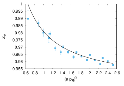
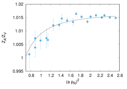
Figure 12: The vector current renormalization factor $Z_{V}$ (top) and the ratio $Z_{A}/Z_{V}$ (bottom) as function of RI-MOM momentum $p_{R}$ in lattice units.

In this appendix, we discuss the calculation of the renormalization of the vector current $Z_{V}$ and axial-vector current $Z_{A}$ in RI-MOM scheme for our setup with $a=0.076$ fm. We use off-shell quark states in the Landau gauge with different values of lattice momenta

$$ap_{\mu}=\frac{2\pi}{L_{\mu}}(n_{\mu}+\frac{1}{2}\delta_{\mu,0}).$$ (75)

To minimize the discretization errors the lattice momenta are substituted by $ap_{\mu}^{\prime}=\sin(ap_{\mu})$, so the renormalization point is $(ap_{R})^{2}=\sum_{\mu=1,4}(ap^{\prime}_{\mu})^{2}$. In Fig. 12, we show our results for $Z_{V}(p_{R})$. The vector current renormalization constant should not depend on $p_{R}$, because in the $a\rightarrow 0$ limit the local current is conserved. Nevertheless, we see a significant dependence on $p_{R}$. This dependence is caused by non-perturbative effects, that for large values of $p_{R}$ can be parameterized by local condensates. As we use off-shell quark states in the Landau gauge in the RI-MOM renormalization procedure, the lowest dimension local condensate is the dimension-two gluon condensate $\langle A^{2}\rangle$ Chetyrkin and Maier (2010); Blossier et al. (2010). Lattice artifact shows up as the breaking of the rotational symmetry on the lattice. We see from Fig. 12 that the fish-bone structure in the lattice data at the level much larger than the statistical errors on $Z_{V}$ for large values of $ap_{R}$. Therefore, to obtain $Z_{V}$ we fit our lattice data with the following form:

$$Z_{V}(p_{R})=Z_{V}+B/(ap_{R})^{2}+C\cdot(ap_{R})^{k}\bigg{(}1+C_{4}\Delta^{(4)}$$ (76)

$$\quad+C_{6}\Delta^{(6)}+C_{8}\Delta^{(8)}\bigg{)},$$ (77)

where

$$\Delta^{(4)}=\frac{\sum_{\mu}(p_{\mu}^{\prime})^{4}}{p_{R}^{4}},~{}\Delta^{(6)}=\frac{\sum_{\mu}(p_{\mu}^{\prime})^{6}}{p_{R}^{6}},~{}\Delta^{(6)}=\frac{\sum_{\mu}(p_{\mu}^{\prime})^{8}}{p_{R}^{8}}.$$ (78)

This form is motivated by the 1-loop lattice perturbation theory Constantinou et al. (2009, 2010) and the perturbative analysis with dimension two gluon condensate Lytle et al. (2018). For the non-perturbative clover action $k=2$, while for Wilson action $k=1$. For HYP smeared clover action with tadpole improved value of $c_{sw}$ we expect ${\cal O}(a)$ discretization errors to be proportional to $\alpha_{s}^{2}$ with a very small coefficient, so it is reasonable to assume that the dominant cutoff effects scale like $a^{2}$. Nevertheless we also perform fits using $k=1$. To limit the size of the lattice artifacts we impose the additional constraint: $\Delta^{(4)}<0.4$. We performed different fits varying the fit interval in $p_{R}$ as well as setting some coefficients to zero in certain cases. Fits with $C=0$ typically have very large $\chi^{2}$ but this has almost no effect of the extracted $Z_{V}$ value. From the fits we obtain $Z_{V}=0.947(8)$, where the error is mostly systematic and corresponds to the scattering of the results from different fits. We could also estimate $Z_{V}$ from the matrix element of the vector charge of the pion calculated in Ref. Gao et al. (2021b). Using the result for the matrix element from the two state fit we obtain $Z_{V}=0.9534(5)$ Gao et al. (2021b). This agrees with the above result within errors.

In Fig. 12 bottom panel, we also show the ratio $Z_{A}/Z_{V}$ as function of $p_{R}$. This ratio too should be independent of $p_{R}$. We see some dependence on $p_{R}$ due to non-perturbative effects, though it is considerably milder than for $Z_{V}$. This is likely due to the fact that the leading non-perturbative contributions cancel out in the ratio $Z_{A}/Z_{V}$. The lattice discretization effects also seem to largely cancel in the ratio $Z_{A}/Z_{V}$ and no clear fish-bone structure can be seen in our data. The $p_{R}$ dependence of $Z_{A}/Z_{V}$ is incompatible with $B/p_{R}^{2}$ form. Therefore, we fit our data with $const+B^{\prime}/(ap_{R})^{4}$ form. This gives $Z_{A}/Z_{V}=1.0168$. For $(ap_{R})^{2}>1.5$ it is also possible to fit the data with constant, which gives $Z_{A}/Z_{V}=1.01514$. Combining these results with the value of $Z_{V}$ from the pion matrix element of the vector charge we obtain $Z_{A}=0.969(1)$. The error is systematic and is due to the difference of the two fits of $Z_{A}/Z_{V}$.

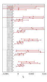
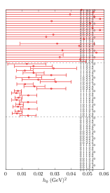
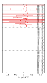
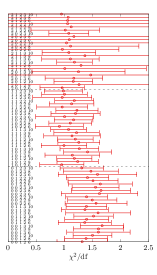
Figure 13: The plot shows additional details of the Mellin moments fit to accompany the values of moments shown in Fig. 6. The specification $(N_{\rm HT},N_{\rm LC},n_{3}^{0},z_{3}^{\rm min}/a,z_{3}^{\rm max}/a)$ is noted on the side of the points, similar to Fig. 6. The first three panels show the best fit values of $l_{0}$, $h_{0}$ and $h_{1}$ respectively – the cases where a parameter is not included is left without a data point. The rightmost panel shows the minimum $\chi^{2}/{\rm df}$ of the fits. The error bar in this case specifies the ranges of $\chi^{2}/{\rm df}$ occuring in the different Jackknife blocks.

Appendix B Details on the Mellin Moments fit

In Section VI.3, we presented the results on the fitted values of the first few Mellin moments based on fits to leading twist Mellin OPE along with lattice correction of the form in Eq. (42) with $l_{2}$ being a fit parameter, and with higher twist corrections in Eq. (43) with $h_{0}$ and $h_{1}$ as possible fit parameters. In this appendix we discuss the results for these additional fit parameters in the Mellin OPE fits with no positivity constraints on the moments. In the first three panels of Fig. 13, we show the scatter of best fit values for $l_{2}$, $h_{0}$ and $h_{1}$ respectively for various fit types specified by $(N_{\rm HT},N_{\rm LC},n_{3}^{0},z_{3}^{\rm min}/a,z_{3}^{\rm max}/a)$ beside the data points. Since certain parameters are not part of all fit types (e.g., $h_{1}$ does not occur when $N_{\rm HT}=0,1$), data points for those cases are left missing in the different panels. From the figure, the conclusions specified in the main text become clearer; namely, the presence of $l_{2}$ has only a marginal effect, whereas the effect of the higher-twist term $h_{0}$ cannot be neglected. Also, $N_{\rm HT}=1$ is sufficient for the fits for the present data quality, whereas inclusion of $h_{1}$ with $N_{\rm HT}=2$ only makes the fits noisier. In the rightmost panel of Fig. 13, we show the scatter of minimum $\chi^{2}/{\rm df}$ in the various fits. The error bars on the minimum $\chi^{2}/{\rm df}$ is obtained from the Jackknife blocks. The mean values of $\chi^{2}/{\rm df}$ for different fits all lie approximately between 1 and 1.6.

References

- Aguilar et al. (2019) A. C. Aguilar et al., Eur. Phys. J. A 55, 190 (2019), arXiv:1907.08218 [nucl-ex] .
- Arrington et al. (2021) J. Arrington et al., J. Phys. G 48, 075106 (2021), arXiv:2102.11788 [nucl-ex] .
- Adams et al. (2018a) B. Adams et al., (2018a), arXiv:1808.00848 [hep-ex] .
- Adams et al. (2018b) B. Adams et al., (2018b), arXiv:1808.00848 [hep-ex] .
- Lepage and Brodsky (1980) G. P. Lepage and S. J. Brodsky, Phys. Rev. D 22, 2157 (1980).
- Lepage and Brodsky (1979) G. P. Lepage and S. J. Brodsky, Phys. Lett. B 87, 359 (1979).
- Efremov and Radyushkin (1980) A. V. Efremov and A. V. Radyushkin, Phys. Lett. B 94, 245 (1980).
- Roberts et al. (2021) C. D. Roberts, D. G. Richards, T. Horn, and L. Chang, Prog. Part. Nucl. Phys. 120, 103883 (2021), arXiv:2102.01765 [hep-ph] .
- Gao et al. (2021a) X. Gao, N. Karthik, S. Mukherjee, P. Petreczky, S. Syritsyn, and Y. Zhao, Phys. Rev. D 103, 094510 (2021a), arXiv:2101.11632 [hep-lat] .
- Behrend et al. (1991) H. J. Behrend et al. (CELLO), Z. Phys. C 49, 401 (1991).
- Gronberg et al. (1998) J. Gronberg et al. (CLEO), Phys. Rev. D 57, 33 (1998), arXiv:hep-ex/9707031 .
- Aubert et al. (2009) B. Aubert et al. (BaBar), Phys. Rev. D 80, 052002 (2009), arXiv:0905.4778 [hep-ex] .
- Uehara et al. (2012) S. Uehara et al. (Belle), Phys. Rev. D 86, 092007 (2012), arXiv:1205.3249 [hep-ex] .
- Melic et al. (2003) B. Melic, D. Mueller, and K. Passek-Kumericki, Phys. Rev. D 68, 014013 (2003), arXiv:hep-ph/0212346 .
- Gao et al. (2022a) J. Gao, T. Huber, Y. Ji, and Y.-M. Wang, Phys. Rev. Lett. 128, 062003 (2022a), arXiv:2106.01390 [hep-ph] .
- Dally et al. (1981) E. B. Dally et al., Phys. Rev. D 24, 1718 (1981).
- Dally et al. (1982) E. B. Dally et al., Phys. Rev. Lett. 48, 375 (1982).
- Amendolia et al. (1984) S. R. Amendolia et al., Phys. Lett. B 146, 116 (1984).
- Amendolia et al. (1986) S. R. Amendolia et al. (NA7), Nucl. Phys. B 277, 168 (1986).
- Volmer et al. (2001) J. Volmer et al. (Jefferson Lab F(pi)), Phys. Rev. Lett. 86, 1713 (2001), arXiv:nucl-ex/0010009 .
- Tadevosyan et al. (2007) V. Tadevosyan et al. (Jefferson Lab F(pi)), Phys. Rev. C 75, 055205 (2007), arXiv:nucl-ex/0607007 .
- Huber et al. (2008) G. M. Huber et al. (Jefferson Lab), Phys. Rev. C 78, 045203 (2008), arXiv:0809.3052 [nucl-ex] .
- Blok et al. (2008) H. P. Blok et al. (Jefferson Lab), Phys. Rev. C 78, 045202 (2008), arXiv:0809.3161 [nucl-ex] .
- Dudek et al. (2012) J. Dudek et al., Eur. Phys. J. A 48, 187 (2012), arXiv:1208.1244 [hep-ex] .
- Farrar and Jackson (1979) G. R. Farrar and D. R. Jackson, Phys. Rev. Lett. 43, 246 (1979).
- Radyushkin (1977) A. V. Radyushkin, (1977), arXiv:hep-ph/0410276 .
- Chernyak and Zhitnitsky (1982) V. L. Chernyak and A. R. Zhitnitsky, Nucl. Phys. B 201, 492 (1982), [Erratum: Nucl.Phys.B 214, 547 (1983)].
- Bakulev et al. (2001) A. P. Bakulev, S. V. Mikhailov, and N. G. Stefanis, Phys. Lett. B 508, 279 (2001), [Erratum: Phys.Lett.B 590, 309–310 (2004)], arXiv:hep-ph/0103119 .
- Agaev et al. (2011) S. S. Agaev, V. M. Braun, N. Offen, and F. A. Porkert, Phys. Rev. D 83, 054020 (2011), arXiv:1012.4671 [hep-ph] .
- Chang et al. (2013a) L. Chang, I. C. Cloet, J. J. Cobos-Martinez, C. D. Roberts, S. M. Schmidt, and P. C. Tandy, Phys. Rev. Lett. 110, 132001 (2013a), arXiv:1301.0324 [nucl-th] .
- Ruiz Arriola and Broniowski (2006) E. Ruiz Arriola and W. Broniowski, Phys. Rev. D 74, 034008 (2006), arXiv:hep-ph/0605318 .
- Kronfeld and Photiadis (1985) A. S. Kronfeld and D. M. Photiadis, Phys. Rev. D 31, 2939 (1985).
- Martinelli and Sachrajda (1987) G. Martinelli and C. T. Sachrajda, Phys. Lett. B 190, 151 (1987).
- DeGrand and Loft (1988) T. A. DeGrand and R. D. Loft, Phys. Rev. D 38, 954 (1988).
- Daniel et al. (1991) D. Daniel, R. Gupta, and D. G. Richards, Phys. Rev. D 43, 3715 (1991).
- Del Debbio et al. (2000) L. Del Debbio, M. Di Pierro, A. Dougall, and C. T. Sachrajda (UKQCD), Nucl. Phys. B Proc. Suppl. 83, 235 (2000), arXiv:hep-lat/9909147 .
- Del Debbio et al. (2003) L. Del Debbio, M. Di Pierro, and A. Dougall, Nucl. Phys. B Proc. Suppl. 119, 416 (2003), arXiv:hep-lat/0211037 .
- Braun et al. (2006) V. M. Braun et al., Phys. Rev. D 74, 074501 (2006), arXiv:hep-lat/0606012 .
- Arthur et al. (2011) R. Arthur, P. A. Boyle, D. Brommel, M. A. Donnellan, J. M. Flynn, A. Juttner, T. D. Rae, and C. T. C. Sachrajda, Phys. Rev. D 83, 074505 (2011), arXiv:1011.5906 [hep-lat] .
- Braun et al. (2015) V. M. Braun, S. Collins, M. Göckeler, P. Pérez-Rubio, A. Schäfer, R. W. Schiel, and A. Sternbeck, Phys. Rev. D 92, 014504 (2015), arXiv:1503.03656 [hep-lat] .
- Bali et al. (2017) G. S. Bali, V. M. Braun, M. Göckeler, M. Gruber, F. Hutzler, P. Korcyl, B. Lang, and A. Schäfer (RQCD), Phys. Lett. B 774, 91 (2017), arXiv:1705.10236 [hep-lat] .
- Bali et al. (2019) G. S. Bali, V. M. Braun, S. Bürger, M. Göckeler, M. Gruber, F. Hutzler, P. Korcyl, A. Schäfer, A. Sternbeck, and P. Wein (RQCD), JHEP 08, 065 (2019), [Addendum: JHEP 11, 037 (2020)], arXiv:1903.08038 [hep-lat] .
- Braun and Müller (2008) V. Braun and D. Müller, Eur. Phys. J. C 55, 349 (2008), arXiv:0709.1348 [hep-ph] .
- Bali et al. (2018a) G. S. Bali et al., Eur. Phys. J. C 78, 217 (2018a), arXiv:1709.04325 [hep-lat] .
- Bali et al. (2018b) G. S. Bali, V. M. Braun, B. Gläßle, M. Göckeler, M. Gruber, F. Hutzler, P. Korcyl, A. Schäfer, P. Wein, and J.-H. Zhang, Phys. Rev. D 98, 094507 (2018b), arXiv:1807.06671 [hep-lat] .
- Ma and Qiu (2018) Y.-Q. Ma and J.-W. Qiu, Phys. Rev. D 98, 074021 (2018), arXiv:1404.6860 [hep-ph] .
- Sufian et al. (2019) R. S. Sufian, J. Karpie, C. Egerer, K. Orginos, J.-W. Qiu, and D. G. Richards, Phys. Rev. D 99, 074507 (2019), arXiv:1901.03921 [hep-lat] .
- Sufian et al. (2020) R. S. Sufian, C. Egerer, J. Karpie, R. G. Edwards, B. Joó, Y.-Q. Ma, K. Orginos, J.-W. Qiu, and D. G. Richards, Phys. Rev. D 102, 054508 (2020), arXiv:2001.04960 [hep-lat] .
- Chambers et al. (2017) A. J. Chambers, R. Horsley, Y. Nakamura, H. Perlt, P. E. L. Rakow, G. Schierholz, A. Schiller, K. Somfleth, R. D. Young, and J. M. Zanotti, Phys. Rev. Lett. 118, 242001 (2017), arXiv:1703.01153 [hep-lat] .
- Detmold and Lin (2006) W. Detmold and C. J. D. Lin, Phys. Rev. D 73, 014501 (2006), arXiv:hep-lat/0507007 .
- Detmold et al. (2021) W. Detmold, A. V. Grebe, I. Kanamori, C. J. D. Lin, R. J. Perry, and Y. Zhao (HOPE), Phys. Rev. D 104, 074511 (2021), arXiv:2103.09529 [hep-lat] .
- Detmold et al. (2022) W. Detmold, A. V. Grebe, I. Kanamori, C. J. D. Lin, S. Mondal, R. J. Perry, and Y. Zhao (HOPE), Phys. Rev. D 105, 034506 (2022), arXiv:2109.15241 [hep-lat] .
- Ji (2013) X. Ji, Phys. Rev. Lett. 110, 262002 (2013), arXiv:1305.1539 [hep-ph] .
- Ji (2014) X. Ji, Sci. China Phys. Mech. Astron. 57, 1407 (2014), arXiv:1404.6680 [hep-ph] .
- Ji et al. (2021a) X. Ji, Y.-S. Liu, Y. Liu, J.-H. Zhang, and Y. Zhao, Rev. Mod. Phys. 93, 035005 (2021a), arXiv:2004.03543 [hep-ph] .
- Radyushkin (2017) A. V. Radyushkin, Phys. Rev. D 96, 034025 (2017), arXiv:1705.01488 [hep-ph] .
- Orginos et al. (2017) K. Orginos, A. Radyushkin, J. Karpie, and S. Zafeiropoulos, Phys. Rev. D 96, 094503 (2017), arXiv:1706.05373 [hep-ph] .
- Radyushkin (2020) A. V. Radyushkin, Int. J. Mod. Phys. A 35, 2030002 (2020), arXiv:1912.04244 [hep-ph] .
- Izubuchi et al. (2019) T. Izubuchi, L. Jin, C. Kallidonis, N. Karthik, S. Mukherjee, P. Petreczky, C. Shugert, and S. Syritsyn, Phys. Rev. D 100, 034516 (2019), arXiv:1905.06349 [hep-lat] .
- Gao et al. (2020) X. Gao, L. Jin, C. Kallidonis, N. Karthik, S. Mukherjee, P. Petreczky, C. Shugert, S. Syritsyn, and Y. Zhao, Phys. Rev. D 102, 094513 (2020), arXiv:2007.06590 [hep-lat] .
- Lin et al. (2021) H.-W. Lin, J.-W. Chen, Z. Fan, J.-H. Zhang, and R. Zhang, Phys. Rev. D 103, 014516 (2021), arXiv:2003.14128 [hep-lat] .
- Gao et al. (2022b) X. Gao, A. D. Hanlon, S. Mukherjee, P. Petreczky, P. Scior, S. Syritsyn, and Y. Zhao, Phys. Rev. Lett. 128, 142003 (2022b), arXiv:2112.02208 [hep-lat] .
- Ji et al. (2015) X. Ji, A. Schäfer, X. Xiong, and J.-H. Zhang, Phys. Rev. D 92, 014039 (2015), arXiv:1506.00248 [hep-ph] .
- Zhang et al. (2017) J.-H. Zhang, J.-W. Chen, X. Ji, L. Jin, and H.-W. Lin, Phys. Rev. D 95, 094514 (2017), arXiv:1702.00008 [hep-lat] .
- Zhang et al. (2019) J.-H. Zhang, L. Jin, H.-W. Lin, A. Schäfer, P. Sun, Y.-B. Yang, R. Zhang, Y. Zhao, and J.-W. Chen (LP3), Nucl. Phys. B 939, 429 (2019), arXiv:1712.10025 [hep-ph] .
- Liu et al. (2019) Y.-S. Liu, W. Wang, J. Xu, Q.-A. Zhang, S. Zhao, and Y. Zhao, Phys. Rev. D 99, 094036 (2019), arXiv:1810.10879 [hep-ph] .
- Zhang et al. (2020) R. Zhang, C. Honkala, H.-W. Lin, and J.-W. Chen, Phys. Rev. D 102, 094519 (2020), arXiv:2005.13955 [hep-lat] .
- Hua et al. (2022) J. Hua et al., (2022), arXiv:2201.09173 [hep-lat] .
- Liu and Dong (1994) K.-F. Liu and S.-J. Dong, Phys. Rev. Lett. 72, 1790 (1994), arXiv:hep-ph/9306299 .
- Izubuchi et al. (2018) T. Izubuchi, X. Ji, L. Jin, I. W. Stewart, and Y. Zhao, Phys. Rev. D 98, 056004 (2018), arXiv:1801.03917 [hep-ph] .
- Braun et al. (2003) V. M. Braun, G. P. Korchemsky, and D. Müller, Prog. Part. Nucl. Phys. 51, 311 (2003), arXiv:hep-ph/0306057 .
- Constantinou and Panagopoulos (2017) M. Constantinou and H. Panagopoulos, Phys. Rev. D 96, 054506 (2017), arXiv:1705.11193 [hep-lat] .
- Chen et al. (2018) J.-W. Chen, T. Ishikawa, L. Jin, H.-W. Lin, Y.-B. Yang, J.-H. Zhang, and Y. Zhao, Phys. Rev. D 97, 014505 (2018), arXiv:1706.01295 [hep-lat] .
- Fan et al. (2020) Z. Fan, X. Gao, R. Li, H.-W. Lin, N. Karthik, S. Mukherjee, P. Petreczky, S. Syritsyn, Y.-B. Yang, and R. Zhang, Phys. Rev. D 102, 074504 (2020), arXiv:2005.12015 [hep-lat] .
- Radyushkin (2019) A. V. Radyushkin, Phys. Rev. D 100, 116011 (2019), arXiv:1909.08474 [hep-ph] .
- (76) DLMF, “NIST Digital Library of Mathematical Functions,” http://dlmf.nist.gov/, Release 1.1.5 of 2022-03-15, f. W. J. Olver, A. B. Olde Daalhuis, D. W. Lozier, B. I. Schneider, R. F. Boisvert, C. W. Clark, B. R. Miller, B. V. Saunders, H. S. Cohl, and M. A. McClain, eds.
- Bazavov et al. (2019) A. Bazavov et al., Phys. Rev. D 100, 094510 (2019), arXiv:1908.09552 [hep-lat] .
- Hasenfratz and Knechtli (2001) A. Hasenfratz and F. Knechtli, Phys. Rev. D 64, 034504 (2001), arXiv:hep-lat/0103029 .
- Bali et al. (2016) G. S. Bali, B. Lang, B. U. Musch, and A. Schäfer, Phys. Rev. D 93, 094515 (2016), arXiv:1602.05525 [hep-lat] .
- Brannick et al. (2008) J. Brannick, R. C. Brower, M. A. Clark, J. C. Osborn, and C. Rebbi, Phys. Rev. Lett. 100, 041601 (2008), arXiv:0707.4018 [hep-lat] .
- Clark et al. (2010) M. A. Clark, R. Babich, K. Barros, R. C. Brower, and C. Rebbi, Comput. Phys. Commun. 181, 1517 (2010), arXiv:0911.3191 [hep-lat] .
- Babich et al. (2011) R. Babich, M. A. Clark, B. Joo, G. Shi, R. C. Brower, and S. Gottlieb, (2011), 10.1145/2063384.2063478, arXiv:1109.2935 [hep-lat] .
- Clark et al. (2016) M. A. Clark, B. Joó, A. Strelchenko, M. Cheng, A. Gambhir, and R. Brower, (2016), arXiv:1612.07873 [hep-lat] .
- Shintani et al. (2015) E. Shintani, R. Arthur, T. Blum, T. Izubuchi, C. Jung, and C. Lehner, Phys. Rev. D 91, 114511 (2015), arXiv:1402.0244 [hep-lat] .
- Gao et al. (2021b) X. Gao, N. Karthik, S. Mukherjee, P. Petreczky, S. Syritsyn, and Y. Zhao, Phys. Rev. D 104, 114515 (2021b), arXiv:2102.06047 [hep-lat] .
- Aoki et al. (2021) Y. Aoki et al., (2021), arXiv:2111.09849 [hep-lat] .
- Tanabashi et al. (2018) M. Tanabashi et al. (Particle Data Group), Phys. Rev. D 98, 030001 (2018).
- Egerer et al. (2022) C. Egerer et al. (HadStruc), Phys. Rev. D 105, 034507 (2022), arXiv:2111.01808 [hep-lat] .
- Karpie et al. (2018) J. Karpie, K. Orginos, and S. Zafeiropoulos, JHEP 11, 178 (2018), arXiv:1807.10933 [hep-lat] .
- Ji et al. (2021b) X. Ji, Y. Liu, A. Schäfer, W. Wang, Y.-B. Yang, J.-H. Zhang, and Y. Zhao, Nucl. Phys. B 964, 115311 (2021b), arXiv:2008.03886 [hep-ph] .
- Gao et al. (2021c) X. Gao, K. Lee, S. Mukherjee, C. Shugert, and Y. Zhao, Phys. Rev. D 103, 094504 (2021c), arXiv:2102.01101 [hep-ph] .
- San Kim et al. (2012) D. San Kim, T. Kim, and S.-H. Rim, Advances in Difference Equations 2012, 1 (2012).
- Braun et al. (2004) V. M. Braun, E. Gardi, and S. Gottwald, Nucl. Phys. B 685, 171 (2004), arXiv:hep-ph/0401158 .
- Ball et al. (2006) P. Ball, V. M. Braun, and A. Lenz, JHEP 05, 004 (2006), arXiv:hep-ph/0603063 .
- Radyushkin (2009) A. V. Radyushkin, Phys. Rev. D 80, 094009 (2009), arXiv:0906.0323 [hep-ph] .
- Karpie et al. (2021) J. Karpie, K. Orginos, A. Radyushkin, and S. Zafeiropoulos (HadStruc), JHEP 11, 024 (2021), arXiv:2105.13313 [hep-lat] .
- Stefanis (2014) N. G. Stefanis, Phys. Lett. B 738, 483 (2014), arXiv:1405.0959 [hep-ph] .
- Stefanis and Pimikov (2016) N. G. Stefanis and A. V. Pimikov, Nucl. Phys. A 945, 248 (2016), arXiv:1506.01302 [hep-ph] .
- Stefanis (2020) N. G. Stefanis, Phys. Rev. D 102, 034022 (2020), arXiv:2006.10576 [hep-ph] .
- Tong et al. (2021) X.-B. Tong, J.-P. Ma, and F. Yuan, Phys. Lett. B 823, 136751 (2021), arXiv:2101.02395 [hep-ph] .
- Tong et al. (2022) X.-B. Tong, J.-P. Ma, and F. Yuan, (2022), arXiv:2203.13493 [hep-ph] .
- Hoodbhoy et al. (2004) P. Hoodbhoy, X.-d. Ji, and F. Yuan, Phys. Rev. Lett. 92, 012003 (2004), arXiv:hep-ph/0309085 .
- Sun et al. (2022) P. Sun, X.-B. Tong, and F. Yuan, Phys. Rev. D 105, 054032 (2022), arXiv:2111.07034 [hep-ph] .
- Chang et al. (2013b) L. Chang, I. C. Cloët, C. D. Roberts, S. M. Schmidt, and P. C. Tandy, Phys. Rev. Lett. 111, 141802 (2013b), arXiv:1307.0026 [nucl-th] .
- Ydrefors et al. (2021) E. Ydrefors, W. de Paula, J. H. A. Nogueira, T. Frederico, and G. Salmé, Phys. Lett. B 820, 136494 (2021), arXiv:2106.10018 [hep-ph] .
- Melic et al. (1999) B. Melic, B. Nizic, and K. Passek, Phys. Rev. D 60, 074004 (1999), arXiv:hep-ph/9802204 .
- Raha and Kohyama (2010) U. Raha and H. Kohyama, Phys. Rev. D 82, 114012 (2010), arXiv:1005.1673 [hep-ph] .
- Pefkou et al. (2022) D. A. Pefkou, D. C. Hackett, and P. E. Shanahan, Phys. Rev. D 105, 054509 (2022), arXiv:2107.10368 [hep-lat] .
- Ji (1995) X.-D. Ji, Phys. Rev. D 52, 271 (1995), arXiv:hep-ph/9502213 .
- Chetyrkin and Maier (2010) K. G. Chetyrkin and A. Maier, Journal of High Energy Physics 2010 (2010), 10.1007/jhep01(2010)092.
- Blossier et al. (2010) B. Blossier, P. Boucaud, F. De soto, V. Morenas, M. Gravina, O. Pene, and J. Rodriguez-Quintero (ETM), Phys. Rev. D 82, 034510 (2010), arXiv:1005.5290 [hep-lat] .
- Constantinou et al. (2009) M. Constantinou, V. Lubicz, H. Panagopoulos, and F. Stylianou, JHEP 10, 064 (2009), arXiv:0907.0381 [hep-lat] .
- Constantinou et al. (2010) M. Constantinou et al. (ETM), JHEP 08, 068 (2010), arXiv:1004.1115 [hep-lat] .
- Lytle et al. (2018) A. Lytle, C. Davies, D. Hatton, G. Lepage, and C. Sturm (HPQCD), Phys. Rev. D 98, 014513 (2018), arXiv:1805.06225 [hep-lat] .