Backward Population Synthesis: Mapping the Evolutionary History of Gravitational-Wave Progenitors

Abstract

One promising way to extract information about stellar astrophysics from gravitational wave catalogs is to compare the catalog to the outputs of stellar population synthesis modeling with varying physical assumptions. The parameter space of physical assumptions in population synthesis is high-dimensional and the choice of parameters that best represents the evolution of a binary system may depend in an as-yet-to-be-determined way on the system’s properties. Here we propose a pipeline to simultaneously infer zero-age main sequence properties and population synthesis parameter settings controlling modeled binary evolution from individual gravitational wave observations of merging compact binaries. Our pipeline can efficiently explore the high-dimensional space of population synthesis settings and progenitor system properties for each system in a catalog of gravitational wave observations. We apply our pipeline to observations in the third third LIGO–Virgo Gravitational-Wave Transient Catalog. We showcase the effectiveness of this pipeline with a detailed study of the progenitor properties and population synthesis settings that produce mergers like the observed GW150914. Our pipeline permits a measurement of the variation of population synthesis parameter settings with binary properties, if any; we present inferences for the recent GWTC-3 transient catalog that suggest that the stable mass transfer efficiency parameter may vary with primary black hole mass.

1 Introduction

As the detection rate of gravitation waves (GWs) from merging double-compact-object (DCO) binaries increases with the sensitivity of the ground-based GW detector network (Aso et al., 2013; LIGO Scientific Collaboration et al., 2015; Acernese et al., 2015; Abbott et al., 2018; Buikema et al., 2020; Tse et al., 2019; Acernese et al., 2019; Akutsu et al., 2021), we are beginning to constrain the astrophysical processes which shape the evolution of GW progenitor populations. One of the most common ways to study progenitor populations of GW mergers is through population synthesis simulations of stellar populations from a host of formation environments. In the case of isolated binary star evolution, merging double compact objects can form from massive binary stars through the standard stable mass transfer or common envelope channels (e.g. Belczynski et al., 2002; Dominik et al., 2012; Belczynski et al., 2016; Stevenson et al., 2017; Zevin et al., 2020; Bavera et al., 2021; Broekgaarden et al., 2021; van Son et al., 2022) as well as through chemically homogenous evolution (Mandel & de Mink, 2016; Marchant et al., 2016; de Mink & Mandel, 2016) or with population III stars (e.g. Belczynski et al., 2004; Kinugawa et al., 2014; Inayoshi et al., 2016, 2017; Tanikawa et al., 2021, 2022). Merging DCO binaries can also originate from a wide variety of dynamically active environments including triple (or higher multiple) systems (e.g. Antonini et al., 2017; Silsbee & Tremaine, 2017; Fragione & Kocsis, 2019; Vigna-Gómez et al., 2021), as well as young stellar clusters (e.g. Ziosi et al., 2014; Banerjee, 2017; Di Carlo et al., 2020; Chattopadhyay et al., 2022), globular clusters (e.g. Portegies Zwart & McMillan, 2000; O’Leary et al., 2006; Downing et al., 2010; Samsing et al., 2014; Rodriguez et al., 2015, 2016; Askar et al., 2017; Rodriguez et al., 2019), nuclear star clusters (Miller & Lauburg, 2009; Antonini & Rasio, 2016), or a mix of all three (e.g. Mapelli et al., 2022). Finally, more exotic channels like active galactic nuclei which combine both gravitational and gas interactions (e.g. McKernan et al., 2018, 2020; Secunda et al., 2020; Ford & McKernan, 2021) or primordial black holes (e.g. Bird et al., 2016; Ali-Haïmoud et al., 2017) can produce merging DCOs observable with a ground-based detector network. For a discussion of the relative rates of each formation environment and channels within, see Mandel & Broekgaarden (2022) and references therein.

Traditionally, population synthesis studies simulate merging DCO populations with a Monte-Carlo approach. Using theoretically motivated distributions of initial parameters like age, metallicity, component mass, orbital separation, and eccentricity, initial populations are evolved with fixed astrophysical assumptions, or population synthesis hyperparameter settings like the stability of Roche-overflow mass transfer, common envelope ejection efficiency, or the strength of compact-object natal kicks, to produce a synthetic catalog of DCO mergers which can be compared to parameterized models derived from observations. This approach relies on several assumptions, both in the simulations and model parameterizations fitted to the GW data, which are unlikely to be fully correct. For example, there is no reason to suppose that the entire population of DCOs should evolve with the same fixed hyperparameters; there is no a priori reason the fitted parameterized model should capture the relevant features of the observed DCO distributions to correspond to the binary physics of interest; etc. A better approach would be to compare progenitor parameters and hyperparameter settings directly to DCO observations, treating the population synthesis model as a mapping from progenitor to merger parameters; merger parameters can then be mapped into observations using a gravitational waveform family, and parameter inference proceeds in the usual way, propagating information back up the mapping chain (e.g. Veitch et al., 2015). A similar methodology, though with fixed hyperparameter settings, was advanced in Andrews et al. (2018, 2021), as we discuss in more detail below.

Attempting to approach such an improved inference procedure for evolutionary hyperparameters using traditional en mass Monte Carlo simulations of entire populations of DCO mergers is computationally infeasible. Even with recent developments in using emulators to speed up the simulation process (e.g. Wong et al., 2021), training the emulators still requires a significant amount of computation to cover a wide range of uncertainty in the hyperparemeter space. As an example, to emulate a model with $10$ parameters, the simplest way to construct a training set of simulations is to run simulations on a grid which varies combinations of uncertain physics. For $10$ uncertain physical processes, if we consider $2$ variations for each physical process this would still require $1024$ simulations. Because population synthesis simulations require hundreds to thousands of cpu hours, training an emulator which spans a high dimensional uncertainty space remains an impossibility at present. Thus inference of hyperpameter settings must proceed dynamically, generating trial DCO systems via population synthesis recipes to match a particular observation one- or few-at-a-time while simultaneously adjusting the hyperparameters. (Eventually it may be even be possible to use more physically-motivated modeling of binary physics (e.g. Gallegos-Garcia et al., 2021) in such a procedure.)

Andrews et al. (2021) (hereafter A21) used DartBoard (Andrews et al., 2018) to determine the ZAMS parameters which produce GW150914-like BBH merger based on posterior samples for GW150914 and a fixed set of hyperparameters which define assumptions for how isolated binary-star interactions proceed using COSMIC, a binary population synthesis code (Breivik et al., 2020). The approach is very similar to the one advocated here except that Andrews et al. (2021) treated the evolutionary hyperparameters for the binary physics as fixed within each analysis. The key extension in this work, which will enable population modeling of both progenitor parameters and hyperparemeter settings, including any possible dependence of hyperparameter settings on progenitor parameters, is to allow these hyperparameters to vary at the same time as intrinsic properties of the progenitor system to produce a joint inference over the intrinsic properties of the progenitor and the necessary hyperparameter settings to produce the observed merger properties.

In full: we propose a method to “backward” model each GW event to its progenitor state while allowing the hyperparameters to vary across their full range of physical uncertainty following a two-stage process. First, we solve a root finding problem to obtain guesses that are likely to produce the desired system properties in the joint progenitor–hyperparameter space. We then sample the posterior in the joint space that is induced by the DCO merger observations using a Markov chain Monte Carlo (MCMC) algorithm that is initialized by the roots found in the previous stage. We demonstrate our algorithm in a realistic setting by producing a posterior over progenitor properties and COSMIC hyperparameters implied by the observation of GW150914.

We find that the progenitor properties and even the ability to produce a GW150914-like merger event is strongly correlated with hyperparameter settings; different assumptions about the black hole masses at merger in GW150914 imply wildly different formation channels and ZAMS progenitor masses for this event and some nearby combinations of ZAMS masses are unable, with any reasonable hyperparameter settings, to produce a DCO merger like GW150914. We further exhibit preliminary results of an ongoing analysis over the entire GWTC-3 catalog (The LIGO Scientific Collaboration et al., 2021) that suggest that the accretion efficiency in stable mass transfer may depend non-trivially on the primary black hole mass in merging systems; our methodology allows for a systematic study of such dependencies, which we will explore more fully in future work.

The rest of the paper is structured as follows: We detail our method in Sec.  2. In Sec.  3, we show the results of applying our method to a number of real events. We discuss the implications of this work and future direction in Sec.  4.

2 Method

We define the progenitor’s zero age main sequence (ZAMS) properties like mass, orbital period, and eccentricity as progenitor parameters $\bm{\theta^{\prime}}$, the parameters that control different uncertain physical prescriptions such as wind strength and common envelope efficiency as hyperparameters $\bm{\lambda}$, and random variables that affect certain stochastic process such as whether CO natal kick unbinds a binary as $\bm{X}$. To avoid clutter in the following derivation, we denote all the parameters related to mapping a particular progenitor system into a GW event collectively as evolutionary parameters $\bm{\Theta}$, which includes $\bm{\theta^{\prime}}$, $\bm{\lambda}$, and $\bm{X}$.

Once all the parameters including a particular draw of all the random variables represented by $\bm{X}$ are known, the population synthesis code is a deterministic function that transforms the properties of the progenitors into the GW parameters $\bm{\theta}$:

$$\bm{\theta}=\bm{f}\left(\bm{\Theta}\right).$$ (1)

The mapping $\bm{f}$ from $\bm{\Theta}$ to $\bm{\theta}$ can be many-to-one due to degeneracies in the different physical processes and initial parameters of the GW event progenitors. In order to draw inferences about $\bm{\Theta}$ from GW data, we must be able to evaluate the likelihood of that data at fixed progenitor parameters, namely

$$p\left(d\mid\bm{\Theta}\right)=p\left(d\mid\bm{\theta}=\bm{f}\left(\bm{\Theta}\right)\right).$$ (2)

The equality holds because the likelihood depends only on the gravitational waveform generated by parameters $\bm{\theta}$ onto which the progenitor parameters map. In principle this likelihood could be computed at arbitrary values of $\bm{\Theta}$ using the same machinery that is used to estimate source parameters in GW catalogs (Veitch et al., 2015; Ashton et al., 2019; Romero-Shaw et al., 2020; The LIGO Scientific Collaboration et al., 2021) to develop samples of progenitor parameters, hyperparameters, and random variables in $\bm{\Theta}$ from a posterior density.

Since the GW likelihood function ultimately depends only on the GW parameters $\theta$, and GWTC-3 already has samples over these parameters from a posterior density

$$p\left(\bm{\theta}\mid d\right)\propto p\left(d\mid\bm{\theta}\right)\pi_{\mathrm{GW}}\left(\bm{\theta}\right),$$ (3)

where $\pi_{\mathrm{GW}}$ is the prior density used for sampling, we can save the computational cost associated with evaluating the GW likelihood by rewriting the posterior density of $\bm{\Theta}$ in terms of the posterior density of $\bm{\theta}$, namely

$$p(\bm{\Theta}|d)=\frac{p(\bm{\theta}(\bm{\Theta})|d)\pi(\bm{\Theta})}{\pi_{\mathrm{GW}}(\bm{\theta}(\bm{\Theta}))}.$$ (4)

We apply a kernel density estimator with a Gaussian kernel to the posterior samples released in GWTC-3 to estimate $p(\bm{\theta}(\bm{\Theta})|d)$.

Including hyperparameters and random variables drastically increases the dimensionality of the problem, which can make the sampling process much more computationally expensive to converge. To speed up the convergence, we first solve a root-finding problem to find points $\bm{\Theta}$ that will generate GW parameters $\bm{\theta}$ close to the bulk of the posterior density of a GW event. We then use those points to initialize a set of chains in the MCMC process.

For each posterior sample point in the GW-observable space, we can find the corresponding evolutionary parameters by solving an optimization problem that minimizes the mean square difference between the GW event parameters and evolutionary parameters as:

$$\mathcal{L}(\bm{\Theta},\bm{\theta})=||f(\bm{\Theta})-\bm{\theta}||^{2}.$$ (5)

In principle, we should only accept solutions that exactly reproduce the LVK posterior samples in the GW-observable space. However, it is not feasible to achieve such a condition in practice, therefore we relax the condition in eq. 5 to a small acceptance threshold. For this study, we picked a threshold of $10^{-2}$. To make sure we find a reasonably complete set of progenitor parameters that corresponds to the posterior sample point, we use 1000 different initial guesses in solving the optimization problem. As long as the solution fulfills the acceptance criteria, the root is as valid as all other roots that fulfill the same acceptance criteria, regardless to its initial guess. This means, we have the freedom to choose the set of initial guesses however we think might benefit the optimization.

Most of the points in the evolutionary parameter space do not produce DCO mergers in a Hubble time. For systems that do not merge, we set the binary masses to be $0$ such that the gradient for the same systems is also $0$ and leads the root finder to get stuck on its first step. Therefore, it is beneficial to choose initial guesses in region of the evolutionary parameter space that are likely to produce DCO mergers. To construct a list of initial guesses, we evolve a set of ZAMS parameters uniformly sampled from the initial binary parameter space, then keep the systems that merge within a Hubble time.

Retaining explicit control over random variables allows us to marginalize over their contribution, and thus allows us to focus on progenitor parameters and hyperparameters. The strength and direction of natal kicks for compact objects are directly specified in the COMPAS binary population synthesis code (Riley et al., 2022) and can also be specified in COSMIC, however this requires the user to specify the strength and direction of natal kicks as inputs through a user-specified pre-processing script. In this study, we use COSMIC in it’s default state which does not specify the kick strength and direction at run time. This means that the process of evolving the binary is not fully deterministic. Thus, even if the root-finding algorithm performs perfectly, forward modelling a set of roots does not guarantee that the simulated population reproduces exactly the set of posterior samples due to randomness in the evolution of each binary. To assure that the recovered progenitor and hyperparameters robustly correspond to the posterior in the GW-observable space, we push forward (or “reproject”) the recovered evolutionary parameters to the GW-observable space to check whether the reprojected posterior agrees with the posterior given by the LVK collaboration.

We use KL divergence to measure the agreement between the two posterior distributions as:

$$D_{KL}(P||Q)=\int P(\bm{x})\log(P(\bm{x})/Q(\bm{x}))dx.$$ (6)

A small KL divergence means the reprojected COSMIC posterior is similar to the original posterior in the observable space, and is thus a viable channel for that specific event. Otherwise, it either means COSMIC can only explain part of the posterior or cannot explain the event at all. This is completely expected behavior since COSMIC, and isolated binary evolution more generally, carries its own assumptions and is expected to fail in reproducing a subset of the event in GWTC-3. One example of this is GW events with at least one component with mass above the pair instability supernova mass limit (Woosley, 2017; Farmer et al., 2019). The reprojection could also be subject to stochasticity in the evolution of each binary. To account for this, we reproject the posterior multiple times with different random seeds and check whether the KL divergence varies significantly. A varying KL divergence means a particular GW event is subject to randomness in the evolution of the progenitor, and extra caution should be used when interpreting the result.

3 Results

Parameters	Description	Optimization range
Observables
$m_{\rm 1,GW}$	Primary mass of the GW event	NA
$m_{\rm 2,GW}$	Secondary mass of the GW event	NA
Progenitor parameters
$m_{\rm 1,ZAMS}$	Primary mass at ZAMS	$[10,150]\ M_{\odot}$
$m_{\rm 2,ZAMS}$	Secondary mass at ZAMS	$[10,150]\ M_{\odot}$
$t_{\rm orb}$	Orbital period at ZAMS	$[5,5000]$ days
$e$	Eccentricity at ZAMS	$[0,1]$
$Z$	Metallicity at ZAMS	$[10^{-4},2\times 10^{-2}]$
$z$	Redshift at ZAMS	NA
hyperparameters
$\alpha$	Common envelope efficiency	$[0.1,10]$
$f_{\rm acc}$	Fraction of accretion during stable mass transfer	$[0,1]$
$q_{\rm crit,3}$	Critical mass ratio on the Hertzsprung Gap	$[0.1,10]$
$\sigma$	Root mean square of Maxwellian natal kick distribution	$[10,300]\ {\rm km/s}$

Table 1: A list of parameters used in this study.

We apply the method described in section 2 to the first GW event GW150914 (Abbott et al., 2016). We use the Overall_posterior posterior samples for GW150914, publicly available from the Gravitational wave Open Science Center (Abbott et al., 2021). The parameters involved in the analysis and the range we allow for the inference are tabulated in table 1. The spin of BHs formed in isolated binaries depends strongly on the angular momentum transport in massive stars which is still highly uncertain (see however Fuller & Ma (2019); Bavera et al. (2020)), therefore we only consider the two component masses in the observable space in both the root-finding stage and the MCMC stage. For progenitor parameters, we characterize each guess with five parameters: the two component masses $M_{\rm 1,ZAMS}$ and $M_{\rm 2,ZAMS}$, the orbital period $t_{\rm orb}$, the eccentricity $e$, and the metallicity $Z$ at ZAMS. Note that the progenitor formation redshift is not obtained through the root-finding process because the formation redshift does not intrinsically affect the evolution of the binary. Instead, we compute the time it takes for the binary to evolve from formation to the merger and add this time to the lookback time when a GW event is observed and limit the total time to merger to be less than $13.7\,\rm{Gyr}$. Using the total lookback time, we can compute the redshift of the binary at ZAMS formation following the Planck 2018 cosmological model (Planck Collaboration et al., 2020). The main benefit of post-processing the redshift in this way is that we do not rely on a particular assumption of star formation rate (SFR) distribution when we solve for the posterior distribution in redshift. This means we can put the prior on formation redshift (or in general, metallicity-redshfit distribution) in by reweighting the posterior distribution according to a particular SFR model, and therefore do not have to rerun the inference every time we change the SFR model. This is especially helpful since SFR models are still highly uncertain but strongly impact the local merger rates of BBHs (e.g. Broekgaarden et al., 2021). For hyperparameters, we choose parameters that strongly affect binary evolution in COSMIC for massive stars, including the common envelope efficiency $\alpha$, the fraction of mass accreted onto the accretor during stable mass transfer $f_{\rm acc}$, the critical mass ratio which determines whether Roche-overflow mass transfer proceeds stably or produces a common envelope when the donor star is on the Hertzsprung gap $q_{\rm crit,3}$, and the root-mean-square of the Maxwellian distribution employed for CO natal kicks, $\sigma$. For systems which begin a common envelope with a Hertzsprung-gap donor, we always assume the pessimistic outcome that the two stars merge since the donor has likely not formed a strong core-envelope boundary (Ivanova & Taam, 2004; Belczynski et al., 2008).

We show a portion of the joint posterior of the progenitor parameters and hyperparameters of GW150914 in figure 1. Each panel is colored based on the comparison between progenitor parameters (blue), hyperparameters (orange), or a mix of the two (green). We find that the choice for $\sigma$ does not affect the formation of GW150914-like BBHs. This is not unexpected since we use the Fryer et al. (2012) delayed model which reduces the natal kick strength at BH formation based on the amount of fallback onto the proto-CO. In the case of GW150914-like BBHs, the BH progenitors are massive enough that the fallback reduces the natal kick to zero. Because of this we do not include $\sigma$ in Figure 1. Similarly, we do not include the ZAMS orbital period and eccentricity, which are correlated with one another, but not strongly with the other progenitor parameters or hyperparameters. We find strong correlations between the ZAMS masses, as well as strong correlations between $M_{2,\rm{ZAMS}}$ and $f_{\rm{acc}}$, and $f_{\rm{acc}}$ and $\alpha$. We show scatter plots of each of these combinations in the upper-right inset of the figure.

The correlations between the ZAMS masses are similar to those found by A21 with the majority of the population preferring primary and secondary masses between $60$–$90\,M_{\odot}$. However, we also find some ZAMS masses which extend up to $150\,M_{\odot}$ which is the limit imposed by our assumptions. We explore the formation scenarios which lead to successful GW150914-like mergers and those which fail to produce GW150914-like mergers below in Figure 2.

The correlations between $M_{2,\rm{ZAMS}}$ and $f_{\rm acc}$ illustrate the variety of ways which GW150914-like mergers can be produced. For binaries with $M_{2,\rm{ZAMS}}<70\,M_{\odot}$, we find that accretion efficiencies of $f_{\rm acc}>0.5$ are preferred. One reason for this is based on the requirement that the total mass in the binary must remain above the total mass of GW150914 and strongly non-conservative mass transfer (i.e. $f_{\rm acc}<0.5$) reduces the total mass of the system. A compounding factor is that as mass leaves the binary due to non-conservative mass transfer, the evolution of the binary’s orbit is less dramatic and leads to wider binaries on average and thus fewer mergers in a Hubble time. For binaries with $M_{2,\rm{ZAMS}}\sim 80\,M_{\odot}$, $f_{\rm acc}$ is less constrained. This is because of a preference for these secondaries to also have primary masses near $80\,M_{\odot}$ and thus enter a double-core common envelope evolution in which both stars’ envelopes are ejected, leaving behind two stripped helium cores in a tight orbit. In this case, $f_{\rm acc}$ does not affect the binary evolution and is thus unconstrained. This effect can also be seen in the ZAMS mass and $q_{\rm crit,3}$ panels for masses near $80\,M_{\odot}$ because double-core common-envelope evolution is triggered in COSMIC when the radii of the two stars touch due to the rapid expansion of the primary star upon helium ignition. In this case, the choice for Roche-overflow mass transfer to proceed stably (as prescribed by $f_{\rm{acc}}$) or unstably (as prescribed by $\alpha$) using $q_{\rm crit,3}$ is totally irrelevant, and thus unconstrained. Finally, for binaries with $M_{2,\rm{ZAMS}}>80$, we find that $f_{\rm acc}$ is correlated to decrease with increasing mass. This is due to limits on the total mass which must be ejected from the binary to produce BH masses that match GW150914, the reverse situation to $M_{2,\rm{ZAMS}}<70\,M_{\odot}$. Binaries with both component masses near $150\,M_{\odot}$ must either go through a common envelope evolution (in which case $f_{\rm acc}$ is unconstrained), or very non-conservative mass transfer (where $f_{\rm acc}$ is low), to produce BBHs with the proper mass.

Finally, we find that $\alpha$ and $f_{\rm acc}$ are largely uncorrelated, though there exist independent trends in each hyper parameter. This is not totally unexpected since the physical processes which are described by each hyperparameter, i.e. stable Roche-lobe overflow and common envelope evolution are two independent channels. Generally, we find that GW150914-like BBHs tend to prefer larger accretion efficiencies and have common envelope ejection efficiencies peaking near $\alpha=1$. One shortcoming of our method implementation is the application of a single hyper parameter for $f_{\mathrm{acc}}$ and $\alpha$ for each binary, while both the primary and the secondary star could in principle be defined by their own hyperparameters that prescribe the outcomes for when each star fills it’s Roche lobe. We reserve full treatment of this for future work but note that this improvement could reveal correlations between hyperparameters that are not present in our current analysis.

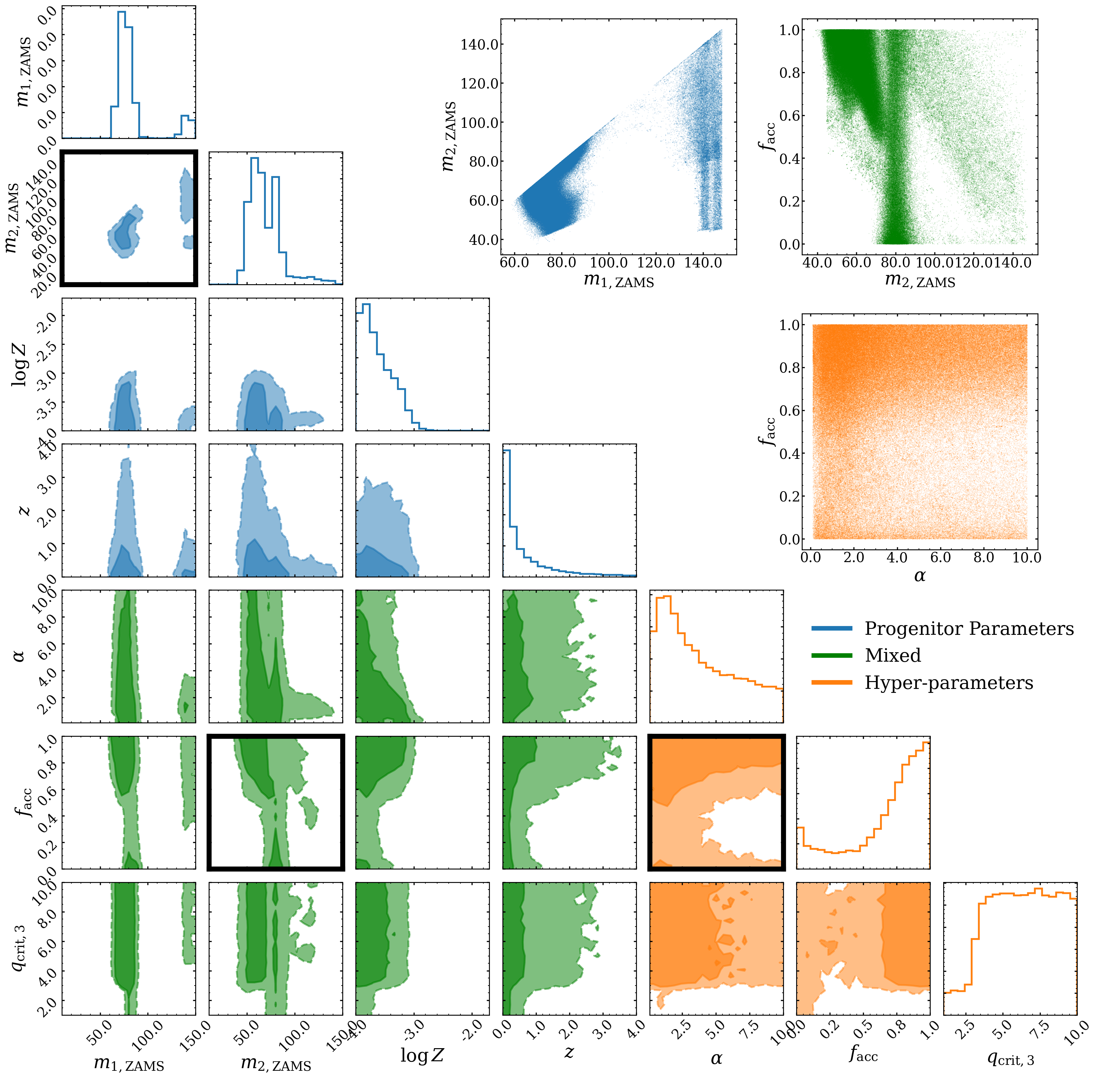
Figure 1: The posterior for GW150914 in both the progenitor parameter space and hyperparameter space. $M_{1}$ and $M_{2}$ are the progenitors’ masses. $\log{Z}$ is log metallicity at ZAMS. $z$ is the redshift at ZAMS. $\alpha$ is the common envelope efficiency. $f_{\rm acc}$ is the fraction of mass accreted during stable mass transfer. $q_{\rm crit,3}$ is the critical mass ratio on the Hertzsprung Gap. The contours correspond to the $68\%$ and $95\%$ confidence intervals. Note that the redshift is not fitted during the root finding process or the MCMC process. Once we find the evolutionary parameters, we add the delay time to the lookback time of the observed posterior sample, then from the total lookback time we can compute the redshift at ZAMS. We highlight three panels in the corner plots to show the fine structure of the set of posterior samples in the evolutionary parameter space. We also color the posterior in a particular panel according to the type of parameters involved in the corner plot. Blue denotes panels that include only progenitor parameters, green denotes panels that include a mix of progenitor parameters and hyperparameters, and orange denotes panels that include only hyperparameters.

Once we obtain a set of binaries which successfully map the ZAMS parameters and hyperparameters to BBH merger masses, we re-evolve the set of ZAMS parameters with the same physical assumptions as A21, but vary the common envelope efficiency to explore how keeping a fixed model which only varies one hyperparameter contrasts to our results. Figure 2 shows the distribution of ZAMS masses for three models (first through third columns), each with a different $\alpha$ but the same hyperparameters as A21, as well as the results of our sampling which allows our hyperparameters to vary (fourth column). We find that holding the accretion efficiency, $f_{\rm{acc}}$, and common envelope ejection efficiency, $\alpha$, to fixed values greatly reduces the ZAMS parameter space that produces GW150914-like mergers. In contrast, by allowing the hyperparameters to fully span the model uncertainty, we find that there are distinct ZAMS parameters which produce GW150914-like mergers.

Because we can explore the full evolutionary parameter space, we can also determine that there are ZAMS parameters which fail to produce GW150914-like mergers regardless of our hyperparameter choice. For primary ZAMS masses between $\sim 95-135\,M_{\odot}$ and secondary ZAMS masses between $\sim 50-95\,M_{\odot}$, we find that there is no combination of accretion efficiency and common envelope ejection efficiency which produces merging BBHs that have masses consistent with GW150914’s posteriors. In this region, if BBHs with masses consistent with GW150914’s masses are produced through a combination of $\alpha$ and $f_{\rm{acc}}$, they do not merge in a Hubble time. Conversely, in the region of the fourth column of Figure 2 which does produce GW150914-like mergers, the combination of $\alpha$, $f_{\rm{acc}}$, and the ZAMS masses and orbital separations balance to produce BHs with the correct masses that merge within a Hubble time.

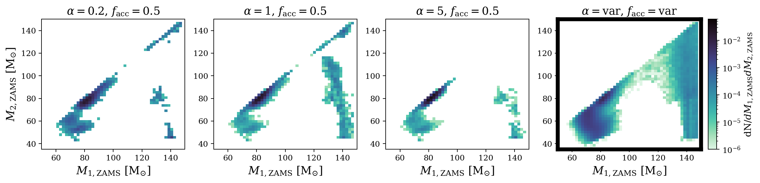
Figure 2: Comparison of ZAMS masses for binaries which produce GW150914-like mergers for three variations of $\alpha$ with a fixed set of parameter assumptions matching those of A21 (first three columns) and for binaries which produce GW150914-like mergers when $\alpha$, $f_{\mathrm{acc}}$, and $q_{crit,3}$ are allowed to vary, (fourth column).

It is interesting to re-project the posterior over progenitor parameters ($\bm{\theta}^{\prime}$) and hyperparameters ($\bm{\lambda}$) using fresh random variables ($\bm{X}$) to the observable space of GW parameters ($\bm{\theta}$). Agreement between the observed parameters and the re-projected parameters indicates good exploration of the random variable space and lack of sensitivity to the details of these random parameters. Figure 3 shows good agreement between the re-projected root-finding outputs as well as the re-projected MCMC draws for our analysis of GW150914. Unlike Andrews et al. (2021), we find there are no regions of observable space inaccessible to our evolutionary models; this difference arises because we allow the evolutionary hyperparameters $\bm{\lambda}$ to vary.

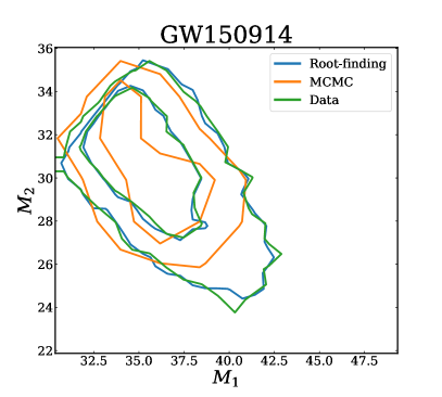
Figure 3: Reprojecting the posterior in evolutionary parameter space of GW150914 to observable space. The contours correspond to the $68\%$ and $95\%$ confidence intervals. The blue contour is the reprojected posterior after the root-finding procedure. The orange contour is the reprojected posterior after the MCMC procedure. The green contour is the posterior plotted using the original LVK posterior samples.

To illustrate the potential benefit of using our method on the population level, we perform the same analysis for all events in GWTC-3. For events announced in GWTC-1, we use Overall_posterior, PublicationSamples,IMRPhenomXPHM_comoving and C01:Mixed posterior samples, respectively. All the data are publicly available from the Gravitational wave Open Science Center (Abbott et al., 2021). Plotted in figure 4 is the posterior density in the $m_{1,{\rm GW}}-f_{\rm acc}$ space for most of the events in GWTC-3. Each contour represents the $68\%$ credible interval of the posterior density for that particular event. There is a suggestive trend showing that $f_{\rm acc}$ could increase as the mass of the progenitor increases. Such a trend implies the stable mass transfer phase of a less massive binary would be preferentially non-conservative, with more conservative mass transfer in more massive binary systems.

Note that some events did not pass the KL divergence test we proposed in section 2; we do not include these systems in figure 4. Binaries that form low-mass compact objects have lower amounts of fallback and tend to have correspondingly larger variance in their random natal kicks. Larger kicks can unbind the progenitor binary, or lead to wide binaries that do not merge within a Hubble time. In these cases, the extra variance during the reprojection can produce a posterior that may not agree with the original posterior, hence yielding a higher KL divergence.

For high-mass binaries, COSMIC struggles to produce events above the pair instability supernova mass cutoff, so the posterior in the evolutionary parameter space only corresponds to part of the posterior in the observable space below this cutoff, and therefore events beyond the lower edge of the PISN mass gap also have higher KL divergence.

Events with more extreme mass ratios are hard to produce with COSMIC, and therefore less likely to be accurately recovered by our method (e.g. Zevin et al., 2020). This could be due to our method assuming a single value for $f_{\rm acc}$ and $\alpha$ as discussed in Section 3.

Merger observations for which COSMIC struggles are likely to be very informative about formation channels and binary evolution physics, and are therefore likely worthy of close study. We anticipate that future work will follow up these events in detail.

Figure 4 shows that our method could in principle reveal the correlation between progenitor parameters and hyperparameters on a population level. Here we impose a cut to eliminate events with KL divergence larger than 0.1. This is a heuristic choice to exclude events that are obviously not compatible with COSMIC. A careful treatment of all events in the catalog and discussion related to the detailed physical implications of figure 4 is beyond the scope of this paper. We defer a detailed study of the physics related to the population of GW events to future work.

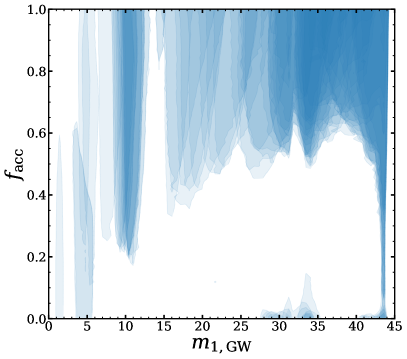
Figure 4: The posterior density in the $m_{1,{\rm GW}}-f_{\rm acc}$ space for most of the events in GWTC-3. Note that $m_{1,{\rm GW}}$ here refers to the reprojected posterior instead of the posterior released by LIGO. Each contour is the $68\%$ credible interval of the posterior density for a particular event. At $m_{1,{\rm GW}}\sim 45M_{\odot}$, the pair instability supernova mechanism prevents COSMIC from producing events that are more massive than this cutoff. Therefore, events with the majority of posterior support above this cutoff are not compatible with COSMIC, hence have a large KL divergence and are excluded from this figure. On the low mass end, neutron star binaries or neutron star-black hole binaries are subjected to randomness induced by the natal kick, also resulting in a larger and fluctuating KL divergences, and therefore are also excluded from the analysis.

4 Discussion

We present a new pathway to understand binary evolution with GW events in this paper. Instead of forward modelling an assumed distribution of initial binaries to the observed population, we find the corresponding evolutionary parameters event-by-event. In this first work, we showcase the power of the proposed method with an application to GW150914. We show the joint posterior of the event’s progenitor parameters and hyperparameters. Our work is both a more efficient way to study GW event progenitors, and also allows the possibility of constraining the astrophysics related to binary evolution, especially by capturing the correlation between hyperparameters in different systems.

Our results suggest that the accretion efficiency during stable mass transfer may depend on the primary black hole mass. In general, our method returns the joint posterior distribution of progenitor parameters and hyperparameters for each event, which enables a data-driven way to study the distribution of hyperparameters. That is, once we have a catalog of events, each has their own posterior in the hyperparameter space, and we can employ well-known techniques such as hierarchical Bayesian analysis to fit a population model to the distribution of hyperparameters; this avoids making overly-specific assumptions like fixing the hyperparameters for all types of event.

Working event-by-event as we do permits post-processing application of arbitrarily complicated models of star formation and metalliticy evolution by re-weighting the samples we obtain (e.g. van Son et al., 2022). Once we have pulled the GW event posterior back from the observable space to the evolutionary parameter space, we can apply the same hierarchical inference methods currently used to infer the compact binary population to our progenitor population. In particular, we can use our progenitor population to infer the formation rate of compact binary population progenitor systems over cosmic time without needing to make artifical and simplistic assumptions about the delay time distribution or the metallicity-specific star formation rate (Vitale et al., 2019; Ng et al., 2021; van Son et al., 2022). Comparing the formation rate of progenitors to the star formation rate provides an avenue to check our understanding of binary evolution and the relative rate of other formation channels.

While our method allows data-driven exploration of the hyperparameters space for the first time, there are a number of improvements that can be implemented in future studies. In this study we use only COSMIC as our evolutionary function, which by design cannot explain all the events in GWTC-3. For example, events with either of the component mass larger than the lower edge of PISN gap such as GW190521 cannot be explained by COSMIC. Alternative channels such as dynamical formation might be needed to explain some subset of the events in GWTC-3 (Zevin et al., 2021). As the sensitivity of GW detectors increases, we expect to see more and more events that are unusual in some way. Therefore, having a self-consistence population synthesis code that contains multiple formation channels is essential to accommodate the growing catalog of GW events. In this paper, our main focus is to illustrate the concept of ”back-propagating” GW-event posterior samples, highlighting the capability of our method and motivating the benefits of building population synthesis codes that can work seamlessly with our method. To avoid cluttering of focus, we discuss the physical implications of the results presented in this work under our specific assumptions (i.e. using COSMIC as our evolutionary function) in a future companion paper.

Due to the implicit definition of random variables in COSMIC, our evolutionary function is stochastic. This introduces significant inefficiency in our root-finding and sampling algorithm. The main stochasticity in COSMIC comes from natal kick, which significantly affect the evolutioary pathway of low mass events such as BNS mergers. The effect of the natal kick is suppressed for heavier mass events due to fallback. This means events with lighter masses are subject to stochasticity of the function, where the sampling process for heavier events behaves as if the evolutionary function we use is deterministic. Due to computational limitation, we only try 1000 different initial guesses per posterior sample in the root-finding process. This means any posterior sample that has a probability of merging rarer than 1 in 1000 could be missed. Obviously the problems which comes with the randomness can be alleviated by performing more tries per posterior sample, but this is not scalable in practice. On top of limitation in efficiency, some formation channels require explicit control of random variables by construction. For example, in a dynamical formation scenario such as binaries that form in a globular cluster, each binary has some probability of undergoing a multi-body encounter with another member in the cluster. These encounter probability distributions are either studied with direct N-body simulations or semi-analytical methods. In both cases, each member of the cluster is no longer completely independent of the other members, but coupled through the encounter probability distribution. By studying the encounter probability distribution, we can infer the properties of the environment which the binary lives in. This can only be done if we have explicit control over the random variables that characterize the encounter probability distribution.

Another technical note is that we use finite differencing to estimate the gradient of the objective function, which could be a significant source of error near transition points in the evolutionary parameter space. Also, finite differencing is increasingly inefficient as we increase the dimensionality of the problem. To improve the accuracy and efficiency in estimating the gradient of the objective function, automatic differentiation is a promising feature that modelers should consider incorporating in their population synthesis codes in the future.

To summarize, we propose a novel method to recover the posterior samples in the evolutionary parameter space for each GW event. We point out hyperparameters in the usual population synthesis simulation context are not actually parameters related to the population, but parameters about the evolutionary function. This means the binary evolution functions can be constrained on an individual event basis. We ”back propagate” the posterior in the observable space to the evolutionary parameter space, thus allowing us to study hyperparameters and theirs correlations with progenitor parameters in a data-driven manner. Our method makes less assumptions than the traditional forward modelling approach, which often fix the hyperparameters across the entire population. Since we are not limited to the fixed hyperparameters assumptions, we can explore the behavior of the hyperparameters across the population much more efficiently. While our work lays down a data analysis pathway to understand the population of GW events, no physics can be learned without a comprehensive physical model. We hope this letter will motivate the construction of next-generation population synthesis codes that have the following properties: first, they should retain explicit control over the random variables so marginalizing over random variables can be done precisely and second, they should be as automatically differentiable as possible so that exploring the evolutionary parameter space is efficient. By combining the methods presented in this work and future, differentiable population synthesis codes, we can explore the full parameter space of binary evolution models with future GW data.

5 Acknowledgement

The authors are grateful for discussions with the CCA Gravitational Wave Astronomy Group. The Flatiron Institute is supported by the Simons Foundation. We thank M. Zevin for helpful comments and suggestions on this manuscript. This research has made use of data or software obtained from the Gravitational Wave Open Science Center (gw-openscience.org), a service of LIGO Laboratory, the LIGO Scientific Collaboration, the Virgo Collaboration, and KAGRA. LIGO Laboratory and Advanced LIGO are funded by the United States National Science Foundation (NSF) as well as the Science and Technology Facilities Council (STFC) of the United Kingdom, the Max-Planck-Society (MPS), and the State of Niedersachsen/Germany for support of the construction of Advanced LIGO and construction and operation of the GEO600 detector. Additional support for Advanced LIGO was provided by the Australian Research Council. Virgo is funded, through the European Gravitational Observatory (EGO), by the French Centre National de Recherche Scientifique (CNRS), the Italian Istituto Nazionale di Fisica Nucleare (INFN) and the Dutch Nikhef, with contributions by institutions from Belgium, Germany, Greece, Hungary, Ireland, Japan, Monaco, Poland, Portugal, Spain. The construction and operation of KAGRA are funded by Ministry of Education, Culture, Sports, Science and Technology (MEXT), and Japan Society for the Promotion of Science (JSPS), National Research Foundation (NRF) and Ministry of Science and ICT (MSIT) in Korea, Academia Sinica (AS) and the Ministry of Science and Technology (MoST) in Taiwan.

References

- Abbott et al. (2016) Abbott, B. P., Abbott, R., Abbott, T. D., et al. 2016, Phys. Rev. Lett., 116, 061102, doi: 10.1103/PhysRevLett.116.061102
- Abbott et al. (2018) Abbott, B. P., Abbott, R., Abbott, T. D., et al. 2018, Living Reviews in Relativity, 21, 3, doi: 10.1007/s41114-018-0012-9
- Abbott et al. (2021) Abbott, R., et al. 2021, SoftwareX, 13, 100658, doi: 10.1016/j.softx.2021.100658
- Acernese et al. (2015) Acernese, F., Agathos, M., Agatsuma, K., et al. 2015, Classical and Quantum Gravity, 32, 024001, doi: 10.1088/0264-9381/32/2/024001
- Acernese et al. (2019) Acernese, F., Agathos, M., Aiello, L., et al. 2019, Phys. Rev. Lett., 123, 231108, doi: 10.1103/PhysRevLett.123.231108
- Akutsu et al. (2021) Akutsu, T., Ando, M., Arai, K., et al. 2021, Progress of Theoretical and Experimental Physics, 2021, 05A101, doi: 10.1093/ptep/ptaa125
- Ali-Haïmoud et al. (2017) Ali-Haïmoud, Y., Kovetz, E. D., & Kamionkowski, M. 2017, Phys. Rev. D, 96, 123523, doi: 10.1103/PhysRevD.96.123523
- Andrews et al. (2021) Andrews, J. J., Cronin, J., Kalogera, V., Berry, C. P. L., & Zezas, A. 2021, ApJ, 914, L32, doi: 10.3847/2041-8213/ac00a6
- Andrews et al. (2018) Andrews, J. J., Zezas, A., & Fragos, T. 2018, ApJS, 237, 1, doi: 10.3847/1538-4365/aaca30
- Antonini & Rasio (2016) Antonini, F., & Rasio, F. A. 2016, ApJ, 831, 187, doi: 10.3847/0004-637X/831/2/187
- Antonini et al. (2017) Antonini, F., Toonen, S., & Hamers, A. S. 2017, ApJ, 841, 77, doi: 10.3847/1538-4357/aa6f5e
- Ashton et al. (2019) Ashton, G., Hübner, M., Lasky, P. D., et al. 2019, ApJS, 241, 27, doi: 10.3847/1538-4365/ab06fc
- Askar et al. (2017) Askar, A., Szkudlarek, M., Gondek-Rosińska, D., Giersz, M., & Bulik, T. 2017, MNRAS, 464, L36, doi: 10.1093/mnrasl/slw177
- Aso et al. (2013) Aso, Y., Michimura, Y., Somiya, K., et al. 2013, Phys. Rev. D, 88, 043007, doi: 10.1103/PhysRevD.88.043007
- Banerjee (2017) Banerjee, S. 2017, MNRAS, 467, 524, doi: 10.1093/mnras/stw3392
- Bavera et al. (2020) Bavera, S. S., Fragos, T., Qin, Y., et al. 2020, A&A, 635, A97, doi: 10.1051/0004-6361/201936204
- Bavera et al. (2021) Bavera, S. S., Fragos, T., Zevin, M., et al. 2021, A&A, 647, A153, doi: 10.1051/0004-6361/202039804
- Belczynski et al. (2004) Belczynski, K., Bulik, T., & Rudak, B. 2004, ApJ, 608, L45, doi: 10.1086/422172
- Belczynski et al. (2002) Belczynski, K., Kalogera, V., & Bulik, T. 2002, ApJ, 572, 407, doi: 10.1086/340304
- Belczynski et al. (2008) Belczynski, K., Kalogera, V., Rasio, F. A., et al. 2008, ApJS, 174, 223, doi: 10.1086/521026
- Belczynski et al. (2016) Belczynski, K., Repetto, S., Holz, D. E., et al. 2016, ApJ, 819, 108, doi: 10.3847/0004-637X/819/2/108
- Bezanson et al. (2017) Bezanson, J., Edelman, A., Karpinski, S., & Shah, V. B. 2017, SIAM Review, 59, 65, doi: 10.1137/141000671
- Bird et al. (2016) Bird, S., Cholis, I., Muñoz, J. B., et al. 2016, Phys. Rev. Lett., 116, 201301, doi: 10.1103/PhysRevLett.116.201301
- Breivik et al. (2020) Breivik, K., Coughlin, S., Zevin, M., et al. 2020, ApJ, 898, 71, doi: 10.3847/1538-4357/ab9d85
- Broekgaarden et al. (2021) Broekgaarden, F. S., Berger, E., Stevenson, S., et al. 2021, arXiv e-prints, arXiv:2112.05763. https://arxiv.org/abs/2112.05763
- Buikema et al. (2020) Buikema, A., Cahillane, C., Mansell, G. L., et al. 2020, Phys. Rev. D, 102, 062003, doi: 10.1103/PhysRevD.102.062003
- Chattopadhyay et al. (2022) Chattopadhyay, D., Hurley, J., Stevenson, S., & Raidani, A. 2022, MNRAS, doi: 10.1093/mnras/stac1163
- de Mink & Mandel (2016) de Mink, S. E., & Mandel, I. 2016, MNRAS, 460, 3545, doi: 10.1093/mnras/stw1219
- Di Carlo et al. (2020) Di Carlo, U. N., Mapelli, M., Giacobbo, N., et al. 2020, MNRAS, 498, 495, doi: 10.1093/mnras/staa2286
- Dominik et al. (2012) Dominik, M., Belczynski, K., Fryer, C., et al. 2012, ApJ, 759, 52, doi: 10.1088/0004-637X/759/1/52
- Downing et al. (2010) Downing, J. M. B., Benacquista, M. J., Giersz, M., & Spurzem, R. 2010, MNRAS, 407, 1946, doi: 10.1111/j.1365-2966.2010.17040.x
- Farmer et al. (2019) Farmer, R., Renzo, M., de Mink, S. E., Marchant, P., & Justham, S. 2019, ApJ, 887, 53, doi: 10.3847/1538-4357/ab518b
- Ford & McKernan (2021) Ford, K. E. S., & McKernan, B. 2021, arXiv e-prints, arXiv:2109.03212. https://arxiv.org/abs/2109.03212
- Foreman-Mackey (2016) Foreman-Mackey, D. 2016, The Journal of Open Source Software, 1, 24, doi: 10.21105/joss.00024
- Fragione & Kocsis (2019) Fragione, G., & Kocsis, B. 2019, MNRAS, 486, 4781, doi: 10.1093/mnras/stz1175
- Fryer et al. (2012) Fryer, C. L., Belczynski, K., Wiktorowicz, G., et al. 2012, ApJ, 749, 91, doi: 10.1088/0004-637X/749/1/91
- Fuller & Ma (2019) Fuller, J., & Ma, L. 2019, ApJ, 881, L1, doi: 10.3847/2041-8213/ab339b
- Gallegos-Garcia et al. (2021) Gallegos-Garcia, M., Berry, C. P. L., Marchant, P., & Kalogera, V. 2021, ApJ, 922, 110, doi: 10.3847/1538-4357/ac2610
- Hunter (2007) Hunter, J. D. 2007, Computing in Science and Engineering, 9, 90, doi: 10.1109/MCSE.2007.55
- Inayoshi et al. (2017) Inayoshi, K., Hirai, R., Kinugawa, T., & Hotokezaka, K. 2017, MNRAS, 468, 5020, doi: 10.1093/mnras/stx757
- Inayoshi et al. (2016) Inayoshi, K., Kashiyama, K., Visbal, E., & Haiman, Z. 2016, MNRAS, 461, 2722, doi: 10.1093/mnras/stw1431
- Ivanova & Taam (2004) Ivanova, N., & Taam, R. E. 2004, ApJ, 601, 1058, doi: 10.1086/380561
- Jones et al. (2001) Jones, E., Oliphant, T., Peterson, P., et al. 2001, SciPy: Open source scientific tools for Python. http://www.scipy.org/
- Kinugawa et al. (2014) Kinugawa, T., Inayoshi, K., Hotokezaka, K., Nakauchi, D., & Nakamura, T. 2014, MNRAS, 442, 2963, doi: 10.1093/mnras/stu1022
- LIGO Scientific Collaboration et al. (2015) LIGO Scientific Collaboration, Aasi, J., Abbott, B. P., et al. 2015, Classical and Quantum Gravity, 32, 074001, doi: 10.1088/0264-9381/32/7/074001
- Luger et al. (2021) Luger, R., Bedell, M., Foreman-Mackey, D., et al. 2021, arXiv e-prints, arXiv:2110.06271. https://arxiv.org/abs/2110.06271
- Mandel & Broekgaarden (2022) Mandel, I., & Broekgaarden, F. S. 2022, Living Reviews in Relativity, 25, 1, doi: 10.1007/s41114-021-00034-3
- Mandel & de Mink (2016) Mandel, I., & de Mink, S. E. 2016, MNRAS, 458, 2634, doi: 10.1093/mnras/stw379
- Mapelli et al. (2022) Mapelli, M., Bouffanais, Y., Santoliquido, F., Arca Sedda, M., & Artale, M. C. 2022, MNRAS, 511, 5797, doi: 10.1093/mnras/stac422
- Marchant et al. (2016) Marchant, P., Langer, N., Podsiadlowski, P., Tauris, T. M., & Moriya, T. J. 2016, A&A, 588, A50, doi: 10.1051/0004-6361/201628133
- McKernan et al. (2020) McKernan, B., Ford, K. E. S., & O’Shaughnessy, R. 2020, MNRAS, 498, 4088, doi: 10.1093/mnras/staa2681
- McKernan et al. (2018) McKernan, B., Ford, K. E. S., Bellovary, J., et al. 2018, ApJ, 866, 66, doi: 10.3847/1538-4357/aadae5
- Miller & Lauburg (2009) Miller, M. C., & Lauburg, V. M. 2009, ApJ, 692, 917, doi: 10.1088/0004-637X/692/1/917
- Ng et al. (2021) Ng, K. K. Y., Vitale, S., Farr, W. M., & Rodriguez, C. L. 2021, ApJ, 913, L5, doi: 10.3847/2041-8213/abf8be
- O’Leary et al. (2006) O’Leary, R. M., Rasio, F. A., Fregeau, J. M., Ivanova, N., & O’Shaughnessy, R. 2006, ApJ, 637, 937, doi: 10.1086/498446
- pandas development team (2020) pandas development team, T. 2020, pandas-dev/pandas: Pandas, 1.1.1, Zenodo, doi: 10.5281/zenodo.3509134
- Planck Collaboration et al. (2020) Planck Collaboration, Aghanim, N., Akrami, Y., et al. 2020, A&A, 641, A6, doi: 10.1051/0004-6361/201833910
- Portegies Zwart & McMillan (2000) Portegies Zwart, S. F., & McMillan, S. L. W. 2000, ApJ, 528, L17, doi: 10.1086/312422
- Riley et al. (2022) Riley, J., Agrawal, P., Barrett, J. W., et al. 2022, ApJS, 258, 34, doi: 10.3847/1538-4365/ac416c
- Rodriguez et al. (2016) Rodriguez, C. L., Chatterjee, S., & Rasio, F. A. 2016, Phys. Rev. D, 93, 084029, doi: 10.1103/PhysRevD.93.084029
- Rodriguez et al. (2015) Rodriguez, C. L., Morscher, M., Pattabiraman, B., et al. 2015, Phys. Rev. Lett., 115, 051101, doi: 10.1103/PhysRevLett.115.051101
- Rodriguez et al. (2019) Rodriguez, C. L., Zevin, M., Amaro-Seoane, P., et al. 2019, Phys. Rev. D, 100, 043027, doi: 10.1103/PhysRevD.100.043027
- Romero-Shaw et al. (2020) Romero-Shaw, I. M., Talbot, C., Biscoveanu, S., et al. 2020, MNRAS, 499, 3295, doi: 10.1093/mnras/staa2850
- Samsing et al. (2014) Samsing, J., MacLeod, M., & Ramirez-Ruiz, E. 2014, ApJ, 784, 71, doi: 10.1088/0004-637X/784/1/71
- Secunda et al. (2020) Secunda, A., Bellovary, J., Mac Low, M.-M., et al. 2020, ApJ, 903, 133, doi: 10.3847/1538-4357/abbc1d
- Silsbee & Tremaine (2017) Silsbee, K., & Tremaine, S. 2017, ApJ, 836, 39, doi: 10.3847/1538-4357/aa5729
- Stevenson et al. (2017) Stevenson, S., Vigna-Gómez, A., Mandel, I., et al. 2017, Nature Communications, 8, 14906, doi: 10.1038/ncomms14906
- Tanikawa et al. (2021) Tanikawa, A., Susa, H., Yoshida, T., Trani, A. A., & Kinugawa, T. 2021, ApJ, 910, 30, doi: 10.3847/1538-4357/abe40d
- Tanikawa et al. (2022) Tanikawa, A., Yoshida, T., Kinugawa, T., et al. 2022, ApJ, 926, 83, doi: 10.3847/1538-4357/ac4247
- The LIGO Scientific Collaboration et al. (2021) The LIGO Scientific Collaboration, the Virgo Collaboration, the KAGRA Collaboration, et al. 2021, arXiv e-prints, arXiv:2111.03606. https://arxiv.org/abs/2111.03606
- Tse et al. (2019) Tse, M., Yu, H., Kijbunchoo, N., et al. 2019, Phys. Rev. Lett., 123, 231107, doi: 10.1103/PhysRevLett.123.231107
- van der Walt et al. (2011) van der Walt, S., Colbert, S. C., & Varoquaux, G. 2011, Computing in Science and Engineering, 13, 22, doi: 10.1109/MCSE.2011.37
- van Son et al. (2022) van Son, L. A. C., de Mink, S. E., Callister, T., et al. 2022, ApJ, 931, 17, doi: 10.3847/1538-4357/ac64a3
- Veitch et al. (2015) Veitch, J., Raymond, V., Farr, B., et al. 2015, Phys. Rev. D, 91, 042003, doi: 10.1103/PhysRevD.91.042003
- Vigna-Gómez et al. (2021) Vigna-Gómez, A., Toonen, S., Ramirez-Ruiz, E., et al. 2021, ApJ, 907, L19, doi: 10.3847/2041-8213/abd5b7
- Vitale et al. (2019) Vitale, S., Farr, W. M., Ng, K. K. Y., & Rodriguez, C. L. 2019, ApJ, 886, L1, doi: 10.3847/2041-8213/ab50c0
- Waskom (2021) Waskom, M. L. 2021, Journal of Open Source Software, 6, 3021, doi: 10.21105/joss.03021
- Wes McKinney (2010) Wes McKinney. 2010, in Proceedings of the 9th Python in Science Conference, ed. Stéfan van der Walt & Jarrod Millman, 56 – 61, doi: 10.25080/Majora-92bf1922-00a
- Wong et al. (2021) Wong, K. W. K., Breivik, K., Kremer, K., & Callister, T. 2021, Phys. Rev. D, 103, 083021, doi: 10.1103/PhysRevD.103.083021
- Woosley (2017) Woosley, S. E. 2017, ApJ, 836, 244, doi: 10.3847/1538-4357/836/2/244
- Zevin et al. (2020) Zevin, M., Spera, M., Berry, C. P. L., & Kalogera, V. 2020, ApJ, 899, L1, doi: 10.3847/2041-8213/aba74e
- Zevin et al. (2021) Zevin, M., Bavera, S. S., Berry, C. P. L., et al. 2021, ApJ, 910, 152, doi: 10.3847/1538-4357/abe40e
- Ziosi et al. (2014) Ziosi, B. M., Mapelli, M., Branchesi, M., & Tormen, G. 2014, MNRAS, 441, 3703, doi: 10.1093/mnras/stu824