1 Introduction

The main ingredient of the axion solution to the strong CP problem [1, 2, 3, 4] is the axion coupling to a pseudo-scalar gluon density, which sets model-independent experimental targets for the axion mass and couplings to photons, nucleons, pions and electrons. Since the axion is much lighter than the scale of chiral symmetry breaking $\Lambda_{\chi}\simeq 1$ GeV and it has the same quantum numbers of the neutral pion, chiral perturbation theory ($\chi$PT) provides a natural framework to systematically derive axion properties. In fact, those were obtained long time ago by using leading order (LO) $\chi$PT (or equivalently current algebra) in a series of renowned papers [3, 5, 6, 7, 8, 9]. The axion chiral potential and coupling to photons at the next-to-LO (NLO) in $\chi$PT were computed in Ref. [10] (see also [11]), but it is only more recently that the program of “precision” axion physics has restarted with Ref. [12], also motivated by the booming of the axion experimental program (see e.g. [13, 14]). State of the art axion mass calculations are now obtained by employing next-to-NLO (NNLO) $\chi$PT [15] or, alternatively, via lattice QCD techniques [16]. The axion-nucleon interaction Lagrangian instead has been derived in heavy baryon $\chi$PT up to NNLO [17, 18]. Also CP- and flavour-violating axion couplings have witnessed a resurgence of interest in the recent years, with new calculations based either on $\chi$PT or other non-perturbative approaches (see respectively Refs. [19, 20, 21, 22] and [23, 24, 25]).

In this paper we focus on the axion-pion chiral Lagrangian at NLO. The latter was previously considered in Refs. [10, 12] in the context of the axion potential, hence limited to non-derivative axion interactions, and more generally in Ref. [26], which included also derivative axion couplings. We here expand on the derivation of the NLO axion-pion chiral Lagrangian, by providing several details which were not presented in Ref. [26].

The most interesting application of this formalism consists in the calculation of the $a\pi\to\pi\pi$ scattering, which provides the dominant channel for axion thermalization in the early Universe [27, 28], when the axion decouples from the thermal bath at temperatures below that of QCD deconfinement $T_{c}\simeq 155$ MeV [29, 30, 31]. The highest attainable axion mass from cosmological constraints on thermally-produced axions is known as the axion hot dark matter bound. However, as shown in Ref. [26], the chiral expansion of the axion-pion thermalization rate breaks down well below $T_{c}$. Lacking for the moment a way to extrapolate the validity of $\chi$PT, a practical solution was given in Refs. [32, 33] which proposed an interpolation of the thermalization rate starting from the high-temperature region above $T_{c}$. See Refs. [34, 35] for recent cosmological analyses adopting this latter approach.

Another application of the axion-pion chiral Lagrangian, which is the main subject of this paper, arises in the context of GeV-scale axion-like particles (ALPs) which dominantly decay hadronically as soon as the phase space for the channel $a\to\pi\pi\pi$ is kinematically open. For phenomenological studies related to this channel, see e.g. Refs. [36, 37, 38]. This process was computed at LO in $\chi$PT in Refs. [39, 40] and the chiral expansion was claimed to be valid up to ALP masses of few GeV. However, by explicitly computing the NLO correction, we find that the effective field theory (EFT) breaks down much earlier, namely for ALP masses just above the kinematical threshold $m_{a}\gtrsim 3m_{\pi}$. Hence, in practice, $\chi$PT never yields an accurate description for the process at hand.

The paper is structured as follows: in Sect. 2 we discuss the construction of the axion-pion chiral Lagrangian, while the calculation of the $a\to\pi\pi\pi$ decay up to NLO in $\chi$PT is outlined in Sect. 3. We conclude in Sect. 4, where we advocate for possible strategies in order to extend the validity of the chiral description. Further details on the NLO calculation are provided in Apps. A–C.

2 Axion-pion effective field theory

The construction of the LO axion-pion Lagrangian was originally discussed in Refs. [6, 9]. We first recall its basic ingredients (see also [27, 39, 41, 40]) in view of the extension at NLO, which was recently discussed in Ref. [26]. We here complement the latter derivation by providing several details which were omitted in Ref. [26]. In particular, we will focus on the 2-flavour formulation, which is best suited for the application to be discussed in Sect. 3. This is justified a posteriori, because the presence of strange mesons as external states is kinematically suppressed up to the energy scale at which the chiral expansion breaks down. On the other hand, the generalization to the 3-flavour case is in principle straightforward. In the following we will generically indicate both the QCD axion and the ALP as “axion”, specifying when needed which case we are considering.

2.1 Axion-QCD effective Lagrangian

The 2-flavour axion effective Lagrangian in terms of quarks and gluons reads

$$\mathcal{L}^{\rm QCD}_{a} =\frac{1}{2}(\partial_{\mu}a)^{2}-\frac{1}{2}m_{a,0}^{2}a^{2}+\frac{\alpha_{s}}{8\pi}\frac{a}{f_{a}}G\widetilde{G}-\overline{q}_{R}M_{q}q_{L}+\text{h.c.}$$

$$+\frac{\partial_{\mu}a}{2f_{a}}\overline{q}c_{q}^{0}\gamma^{\mu}\gamma_{5}q+\frac{1}{4}g^{0}_{a\gamma}aF\tilde{F}\,,$$ (2.1)

where $q=(u,d)^{T}$, $M_{q}=\mbox{diag}\,(m_{u},m_{d})$, $G\widetilde{G}\equiv\frac{1}{2}\epsilon^{\mu\nu\rho\sigma}G^{A}_{\mu\nu}G^{A}_{\rho\sigma}$ and $F\widetilde{F}\equiv\frac{1}{2}\epsilon^{\mu\nu\rho\sigma}F_{\mu\nu}F_{\rho\sigma}$, with $\epsilon^{0123}=-1$. For the QCD axion $m_{a,0}^{2}=0$, while $m_{a,0}^{2}\neq 0$ for the ALP case. In the following, we will be especially interested in the case where $m_{a,0}\sim$ GeV, i.e. much larger than the pure QCD axion mass contribution. The couplings $c^{0}_{q}=\text{diag}(c^{0}_{u},c^{0}_{d})$ and $g^{0}_{a\gamma}$ are model-dependent. For instance, in the case of the QCD axion, $c^{0}_{u,d}=0$ and $g^{0}_{a\gamma}=0$ in the KSVZ model [42, 43], while $c^{0}_{u}=\frac{1}{3}\cos^{2}\beta$, $c^{0}_{d}=\frac{1}{3}\sin^{2}\beta$ and $g^{0}_{a\gamma}=\alpha/(2\pi f_{a})8/3$ in the DFSZ model [44, 45] (with $\tan\beta=v_{u}/v_{d}$ the ratio between the vacuum expectation values of the two Higgs doublets present in the DFSZ model).

Upon an anomalous axial rotation of the quark doublet

$$q\rightarrow e^{i\gamma_{5}\frac{a}{2f_{a}}Q_{a}}q\,,$$ (2.2)

with $\mbox{Tr}\,Q_{a}=1$, the $aG\tilde{G}$ term in Eq. (2.1) is shifted away, and the Lagrangian in Eq. (2.1) becomes

$$\mathcal{L}^{\rm QCD}_{a}=\frac{1}{2}(\partial_{\mu}a)^{2}-\frac{1}{2}m_{a,0}^{2}a^{2}-(\overline{q}_{R}M_{a}q_{L}+\text{h.c.})+\frac{\partial_{\mu}a}{2f_{a}}\overline{q}c_{q}\gamma^{\mu}\gamma_{5}q+\frac{1}{4}g_{a\gamma}aF\widetilde{F}\,,$$ (2.3)

where we have redefined the parameters as

$$M_{a}=e^{-i\frac{a}{2f_{a}}Q_{a}}M_{q}e^{-i\frac{a}{2f_{a}}Q_{a}}\,,\quad c_{q}=c_{q}^{0}-Q_{a}\,,\quad g_{a\gamma}=g^{0}_{a\gamma}-\frac{3\alpha}{2\pi f_{a}}\mbox{Tr}\,(Q_{a}Q_{\rm EM}^{2})\,,$$ (2.4)

with $Q_{\rm EM}=\mbox{diag}\,(2/3,-1/3)$.

2.2 Axion-pion effective Lagrangian at LO

At energies $\lesssim$ 1 GeV, the axion-QCD effective Lagrangian is replaced by the axion chiral Lagrangian, which at the LO reads (in the 2-flavour approximation, relevant for the observable studied in this paper)

$$\mathcal{L}^{\chi({\rm LO})}_{a} =\frac{1}{2}(\partial_{\mu}a)^{2}-\frac{1}{2}m_{a,0}^{2}a^{2}+\frac{f_{\pi}^{2}}{4}\mbox{Tr}\left[(D^{\mu}U)^{\dagger}D_{\mu}U+U\chi^{\dagger}_{a}+\chi_{a}U^{\dagger}\right]$$

$$+\frac{\partial^{\mu}a}{2f_{a}}\mbox{Tr}\left[c_{q}\sigma^{a}\right]J^{a}_{A,\,\mu}|_{\rm LO}\,,$$ (2.5)

where $f_{\pi}=92.21\ \rm MeV$, $\chi_{a}=2B_{0}M_{a}$ (with $B_{0}$ denoting the quark condensate) and $\sigma^{a}$ ($a=1,2,3$) the Pauli matrices. $U=e^{i\pi^{a}\sigma^{a}/f_{\pi}}$ is the pion Goldstone matrix, with

$$\pi^{a}\sigma^{a}=\begin{pmatrix}\pi_{0}&\sqrt{2}\pi_{+}\\ \sqrt{2}\pi_{-}&-\pi_{0}\end{pmatrix}\,.$$ (2.6)

The pion axial current, $J^{a}_{A,\,\mu}$, reads at the LO (see App. A)

$$J^{a}_{A,\,\mu}|_{\rm LO}=\frac{i}{4}f_{\pi}^{2}\mbox{Tr}\left[\sigma^{a}\{U,(D_{\mu}U)^{\dagger}\}\right]\,,$$ (2.7)

defined in terms of the covariant derivative $D_{\mu}U=\partial_{\mu}U-ir_{\mu}U+iU\ell_{\mu}$, with $r_{\mu}=r_{\mu}^{a}\sigma^{a}/2$ and $l_{\mu}=l_{\mu}^{a}\sigma^{a}/2$ external fields which can be used to include electromagnetic or weak effects. The matching of the derivative axion term in Eq. (2.2) with the corresponding one in Eq. (2.3) has been obtained by rewriting

$$\overline{q}_{i}[c_{q}]_{ij}\gamma^{\mu}\gamma_{5}q_{j}=\frac{1}{2}\Big{(}\mbox{Tr}\,[c_{q}]\underbrace{\overline{q}\gamma^{\mu}\gamma_{5}q}_{\rm iso-singlet}+\mbox{Tr}\,[c_{q}\sigma^{a}]\underbrace{\overline{q}\gamma^{\mu}\gamma_{5}\tfrac{\sigma^{a}}{2}q}_{\rm iso-triplet}\Big{)}\,,$$ (2.8)

where we used the Fierz identity $\sigma^{a}_{ij}\sigma^{a}_{kl}=2(\delta_{il}\delta_{jk}-\frac{1}{2}\delta_{ij}\delta_{kl})$. The iso-singlet current is associated to the heavy $\eta^{\prime}$ and it can be neglected for our purposes, while the iso-triplet quark axial current is replaced with the pion axial current in Eq. (2.7).

In the following, we set $Q_{a}=M_{q}^{-1}/\mbox{Tr}\,M_{q}^{-1}$, so that terms linear in $a$ (including $a$-$\pi^{0}$ mass mixing) drop out from Eq. (2.2) and the only linear axion term arise from the derivative interaction with the pion axial current. Explicitly, the derivative axion coupling reads

$$\mbox{Tr}\left[c_{q}\sigma^{a}\right]=\left(\frac{m_{u}-m_{d}}{m_{u}+m_{d}}+c^{0}_{u}-c^{0}_{d}\right)\delta^{a3}\,.$$ (2.9)

Expanding the pion axial current $J_{A,\,\mu}^{a}|_{\rm LO}=f_{\pi}\partial_{\mu}\pi^{a}-\frac{1}{f_{\pi}}\pi^{2}\partial_{\mu}\pi^{a}-\frac{3}{2f_{\pi}}\pi^{a}\partial_{\mu}\pi^{2}+\ldots\$, with $\pi=\sqrt{\pi_{0}\pi_{0}+2\pi_{+}\pi_{-}}$, the axion-pion derivative terms are given by

$$\frac{\partial^{\mu}a}{2f_{a}} {\rm Tr}\left[c_{q}\sigma^{a}\right]J^{a}_{A,\,\mu}|_{\rm LO}\simeq-\frac{1}{2}\Bigg{(}\frac{m_{d}-m_{u}}{m_{u}+m_{d}}+c_{d}^{0}-c_{u}^{0}\Bigg{)}\frac{f_{\pi}}{f_{a}}\partial_{\mu}a\partial^{\mu}\pi_{0}$$ (2.10)

$$+ \frac{1}{3}\Bigg{(}\frac{m_{d}-m_{u}}{m_{u}+m_{d}}+c_{d}^{0}-c_{u}^{0}\Bigg{)}\frac{1}{f_{a}f_{\pi}}\partial_{\mu}a\Big{(}2\partial^{\mu}\pi_{0}\pi_{+}\pi_{-}-\pi_{0}\partial^{\mu}\pi_{+}\pi_{-}-\pi_{0}\pi_{+}\partial^{\mu}\pi_{-}\Big{)}\,.$$

The first operator introduces a kinetic mixing between the axion and the neutral pion, parametrized by the coefficient

$$\epsilon\equiv-\frac{1}{2}\frac{f_{\pi}}{f_{a}}\left(\frac{m_{d}-m_{u}}{m_{d}+m_{u}}+c_{d}^{0}-c_{u}^{0}\right)\,.$$ (2.11)

At the quadratic level the $a$-$\pi^{0}$ Lagrangian reads

$$\mathcal{L}_{a-\pi_{0}}^{\rm quad}=\frac{1}{2}\left(\partial_{\mu}a\quad\partial_{\mu}\pi_{0}\right)\mathcal{K}_{\rm LO}\begin{pmatrix}\partial^{\mu}a\\ \partial^{\mu}\pi_{0}\end{pmatrix}-\frac{1}{2}\left(a\quad\pi_{0}\right)\mathcal{M}^{2}_{\rm LO}\begin{pmatrix}a\\ \pi_{0}\end{pmatrix}\,,$$ (2.12)

with

$$\mathcal{K}_{\rm LO}=\begin{pmatrix}1&\epsilon\\ \epsilon&1\end{pmatrix},\qquad\mathcal{M}^{2}_{\rm LO}=\begin{pmatrix}m_{a}^{2}&0\\ 0&m_{\pi}^{2}\end{pmatrix}$$ (2.13)

and $m_{a}^{2}=m_{a,0}^{2}+m_{a,\text{QCD}}^{2}$, where

$$m_{a,\text{QCD}}^{2}=\frac{m_{u}m_{d}}{(m_{u}+m_{d})^{2}}\frac{m_{\pi}^{2}f_{\pi}^{2}}{f_{a}^{2}}\simeq 5.7\Bigg{(}\frac{10^{12}\ \text{GeV}}{f_{a}}\Bigg{)}\ {\rm\mu eV}\,,$$ (2.14)

is the QCD axion mass squared at the LO. The procedure in order to diagonalize the quadratic Lagrangian in Eq. (2.12) consists of three steps: $i)$ diagonalization of the kinetic term by an orthogonal transformation, $ii)$ re-scaling of the fields to have a canonical kinetic term and $iii)$ diagonalization of the mass matrix (rotated and re-scaled after steps $i)$ and $ii)$). The first orthogonal rotation

$$R_{1}=\frac{1}{\sqrt{2}}\begin{pmatrix}-1&1\\ 1&1\end{pmatrix}$$ (2.15)

gives

$$R_{1}^{T}\mathcal{K}_{\rm LO}R_{1}=\begin{pmatrix}1-\epsilon&0\\ 0&1+\epsilon\end{pmatrix}\,.$$ (2.16)

Therefore the re-scaling is given by (fields need to be multiplied by the inverse of $W$)

$$W=\begin{pmatrix}\frac{1}{\sqrt{1-\epsilon}}&0\\ 0&\frac{1}{\sqrt{1+\epsilon}}\end{pmatrix}\,.$$ (2.17)

The action of $R_{1}$ and $W$ on the mass matrix puts it in the form

$$\hat{\mathcal{M}}^{2}_{\rm LO}=WR_{1}^{T}\mathcal{M}_{\rm LO}^{2}R_{1}W=\frac{1}{2}\begin{pmatrix}\dfrac{m_{a}^{2}+m_{\pi}^{2}}{1-\epsilon}&\dfrac{m_{\pi}^{2}-m_{a}^{2}}{\sqrt{1-\epsilon^{2}}}\\ \dfrac{m_{\pi}^{2}-m_{a}^{2}}{\sqrt{1-\epsilon^{2}}}&\dfrac{m_{a}^{2}+m_{\pi}^{2}}{1+\epsilon}\\ \end{pmatrix}\,,$$ (2.18)

whose eigenvalues are $m_{\pi}^{2}$ and $m_{a}^{2}$ plus corrections of $O(\epsilon^{2})$ for the pion and ALP masses, and $O(\epsilon^{4})$ for the QCD axion mass (considering $m_{a}/m_{\pi}\sim\mathcal{O}(\epsilon)$ in the QCD axion case). Denoting by $R_{2}$ the matrix that diagonalizes Eq. (2.18) as $R_{2}^{T}\hat{\mathcal{M}}^{2}_{\rm LO}R_{2}$, one obtains that the complete rotation that needs to be applied to the fields $(a,\pi_{0})$ in order to fully diagonalize the quadratic Lagrangian in Eq. (2.12) is given by

$$\mathcal{R}=\left(R_{1}WR_{2}\right)^{-1}=\begin{pmatrix}1-\dfrac{\epsilon^{2}m_{a}^{4}}{2(m_{a}^{2}-m_{\pi}^{2})^{2}}&-\dfrac{\epsilon m_{\pi}^{2}}{m_{a}^{2}-m_{\pi}^{2}}\\ \dfrac{\epsilon m_{a}^{2}}{m_{a}^{2}-m_{\pi}^{2}}&1+\dfrac{\epsilon^{2}m_{\pi}^{4}}{2(m_{a}^{2}-m_{\pi}^{2})^{2}}\\ \end{pmatrix}\,.$$ (2.19)

Neglecting $\mathcal{O}(\epsilon^{2})$ terms in $\mathcal{R}^{-1}$, we finally obtain

$$a =a_{\rm phys}+\dfrac{\epsilon m_{\pi}^{2}}{m_{a}^{2}-m_{\pi}^{2}}{\pi_{0}}_{\rm phys}\,,$$ (2.20)

$$\pi_{0} ={\pi_{0}}_{\rm phys}-\dfrac{\epsilon m_{a}^{2}}{m_{a}^{2}-m_{\pi}^{2}}a_{\rm phys}\,,$$ (2.21)

where ($a_{\rm phys}$, ${\pi_{0}}_{\rm phys}$) denote fields with diagonal propagators. In the following, we drop the subscript “phys” when working in the diagonal basis.

After the LO diagonalization procedure, the LO chiral Lagrangian containing the axion-pions interaction terms is given by (including the contribution due to Eq. (2.21) from the standard 4-pion Lagrangian)

$$\mathcal{L}_{a\pi}^{\chi({\rm LO})}=\frac{C_{a\pi}}{2f_{a}f_{\pi}(m_{a}^{2}-m_{\pi}^{2})}\Big{\{}(m_{a}^{2}-2m_{\pi}^{2})\,\partial_{\mu}a\Big{(}2\partial_{\mu}\pi_{0}\pi_{+}\pi_{-}-\pi_{0}\partial_{\mu}\pi_{+}\pi_{-}-\pi_{0}\pi_{+}\partial_{\mu}\pi_{-}\Big{)}$$

$$+m_{a}^{2}\,a\Big{(}m_{\pi}^{2}(\pi_{0}\pi_{+}\pi_{-}+\frac{1}{2}\pi_{0}^{3})-2\pi_{0}\partial_{\mu}\pi_{+}\partial^{\mu}\pi_{-}+\partial_{\mu}\pi_{0}\left(\partial^{\mu}\pi_{+}\pi_{-}+\partial^{\mu}\pi_{-}\pi_{+}\right)\Big{)}\Big{\}}\,,$$ (2.22)

with

$$C_{a\pi}=\frac{1}{3}\Bigg{(}\frac{m_{d}-m_{u}}{m_{u}+m_{d}}+c_{d}^{0}-c_{u}^{0}\Bigg{)}\,.$$ (2.23)

The QCD axion case is recovered in the $m_{a}^{2}\to 0$ limit. Note that the correction due to the kinetic mixing in Eq. (2.21) can be safely neglected in the QCD axion case since $m_{a}\ll m_{\pi}$.

2.3 Axion-pion effective Lagrangian at NLO

The axion-pion Lagrangian beyond LO requires two ingredients: the $\mathcal{O}(p^{4})$ chiral Lagrangian with the axion-dressed coefficient $\chi_{a}=2B_{0}M_{a}$ (cf. Eq. (2.4)) and the derivative axion interaction with the NLO pion axial current. Part of the material of this Section was previously presented in Ref. [26]. The 2-flavour chiral Lagrangian at $\mathcal{O}(p^{4})$ can be expressed in various equivalent bases. Here we stick to the expression given by Gasser and Leutwyler [46], which in the standard trace notation reads [47]

$$\mathcal{L}^{\chi({\rm NLO})}_{a}=\frac{\ell_{1}}{4}\left\{\operatorname{{\rm Tr}}\left[D_{\mu}U\left(D^{\mu}U\right)^{\dagger}\right]\right\}^{2}+\frac{\ell_{2}}{4}\operatorname{{\rm Tr}}\left[D_{\mu}U\left(D_{\nu}U\right)^{\dagger}\right]\operatorname{{\rm Tr}}\left[D^{\mu}U\left(D^{\nu}U\right)^{\dagger}\right]$$

$$+\frac{\ell_{3}}{16}\left[\operatorname{{\rm Tr}}\left(\chi_{a}U^{\dagger}+U\chi_{a}^{\dagger}\right)\right]^{2}+\frac{\ell_{4}}{4}\operatorname{{\rm Tr}}\left[D_{\mu}U\left(D^{\mu}\chi_{a}\right)^{\dagger}+D_{\mu}\chi_{a}\left(D^{\mu}U\right)^{\dagger}\right]$$

$$+\ell_{5}\left[\operatorname{{\rm Tr}}\left(f_{\mu\nu}^{R}Uf_{L}^{\mu\nu}U^{\dagger}\right)-\frac{1}{2}\operatorname{{\rm Tr}}\left(f_{\mu\nu}^{L}f_{L}^{\mu\nu}+f_{\mu\nu}^{R}f_{R}^{\mu\nu}\right)\right]$$

$$+i\frac{\ell_{6}}{2}\operatorname{{\rm Tr}}\left[f_{\mu\nu}^{R}D^{\mu}U\left(D^{\nu}U\right)^{\dagger}+f_{\mu\nu}^{L}\left(D^{\mu}U\right)^{\dagger}D^{\nu}U\right]$$

$$-\frac{\ell_{7}}{16}\left[\operatorname{{\rm Tr}}\left(\chi_{a}U^{\dagger}-U\chi_{a}^{\dagger}\right)\right]^{2}+\frac{h_{1}+h_{3}}{4}\operatorname{{\rm Tr}}\left(\chi_{a}\chi_{a}^{\dagger}\right)+\frac{h_{1}-h_{3}}{16}\left\{\left[\operatorname{{\rm Tr}}\left(\chi_{a}U^{\dagger}+U\chi_{a}^{\dagger}\right)\right]^{2}\right.$$

$$\left.+\left[\operatorname{{\rm Tr}}\left(\chi_{a}U^{\dagger}-U\chi_{a}^{\dagger}\right)\right]^{2}-2\operatorname{{\rm Tr}}\left(\chi_{a}U^{\dagger}\chi_{a}U^{\dagger}+U\chi_{a}^{\dagger}U\chi_{a}^{\dagger}\right)\right\}-2h_{2}\operatorname{{\rm Tr}}\left(f_{\mu\nu}^{L}f_{L}^{\mu\nu}+f_{\mu\nu}^{R}f_{R}^{\mu\nu}\right)$$

$$+\frac{\partial^{\mu}a}{2f_{a}}\mbox{Tr}\left[c_{q}\sigma^{a}\right]J^{a}_{A,\,\mu}|_{\rm NLO}\,.$$ (2.24)

The low-energy constants $\ell_{1},\ell_{2},\ldots,\ell_{7}$ are not fixed by chiral symmetry, but they need to be determined from experimental data or lattice QCD. The constants $h_{1}$, $h_{2}$, $h_{3}$ are coupled to pion-independent terms (see Eq. (2.3) below). The $f_{\mu\nu}^{R,L}$ are the field strength tensors associated to the fields $r_{\mu}$ and $l_{\mu}$ appearing in the covariant derivative (see [46] for details). Since we are only interested in processes involving an even number of bosons, we neglect here the $\mathcal{O}(p^{4})$ Wess-Zumino-Witten term [48, 49] which features intrinsic-parity-odd operators.

The NLO chiral left (right) current is obtained by differentiating the NLO Lagrangian with respect to the external field $l_{\mu}$ ($r_{\mu}$). Taking the axial combination of the chiral currents (see App. A) one obtains

$$J^{a}_{A,\,\mu}|_{\rm NLO} =i\frac{\ell_{1}}{2}\mbox{Tr}\left[\sigma^{a}\{D_{\mu}U^{\dagger},U\}\right]\mbox{Tr}\left[D_{\nu}UD^{\nu}U^{\dagger}\right]$$ (2.25)

$$+i \frac{\ell_{2}}{4}\mbox{Tr}\left[\sigma^{a}\{D^{\nu}U^{\dagger},U\}\right]\mbox{Tr}\left[D_{\mu}UD_{\nu}U^{\dagger}+D_{\nu}UD_{\mu}U^{\dagger}\right]$$

$$-i \frac{\ell_{4}}{8}\mbox{Tr}\left[\sigma^{a}\{D_{\mu}U,\chi^{\dagger}_{a}\}-\sigma^{a}\{U,D_{\mu}\chi^{\dagger}_{a}\}+\sigma^{a}\{D_{\mu}\chi_{a},U^{\dagger}\}-\sigma^{a}\{\chi_{a},D_{\mu}U^{\dagger}\}\right]$$

$$+ \frac{\ell_{6}}{4}\mbox{Tr}\left[f_{\mu\nu}^{R}[\sigma^{a},D^{\nu}U]U^{\dagger}+f_{\mu\nu}^{R}U[D^{\nu}U^{\dagger},\sigma^{a}]+f_{\mu\nu}^{L}U^{\dagger}[\sigma^{a},D^{\nu}U]+f_{\mu\nu}^{L}[D^{\nu}U^{\dagger},\sigma^{a}]U\right]\,.$$

Being interested only in axion-pion interactions, from now on we will set to zero the field strength tensors as well as the external currents. Then the axion-pion Lagrangian up to NLO is given by the sum $\mathcal{L}^{\chi({\rm LO})}_{a}+\mathcal{L}^{\chi({\rm NLO})}_{a}$.

Note that the NLO terms reintroduce a quadratic mixing of the axion field with the neutral pion. In App. B we explicitly repeat the diagonalization procedure at NLO, including as well one-loop terms from the LO chiral Lagrangian. In fact, the choice $Q_{a}=M_{q}^{-1}/{\rm Tr}\,M_{q}^{-1}$ allows us to eliminate only some of the mass mixing terms at NLO. On the other hand, no axion-pion mixing arises from the term proportional to $h_{1}-h_{3}$ in Eq. (2.3), since the latter does not depend on the pion field. This is readily seen by using the identity

$$\left[{\rm Tr}\left(\chi_{a}U^{\dagger}+U\chi^{\dagger}_{a}\right)\right]^{2}+\left[{\rm Tr}\left(\chi_{a}U^{\dagger}-U\chi^{\dagger}_{a}\right)\right]^{2}-2{\rm Tr}\left(\chi_{a}U^{\dagger}\chi_{a}U^{\dagger}+U\chi^{\dagger}_{a}U\chi^{\dagger}_{a}\right)$$

$$=\left[{\rm Tr}(\chi_{a})\right]^{2}+\left[{\rm Tr}(\chi^{\dagger}_{a})\right]^{2}-\left[{\rm Tr}(\sigma^{a}\chi_{a})\right]^{2}-\left[{\rm Tr}(\sigma^{a}\chi^{\dagger}_{a})\right]^{2}\,.$$ (2.26)

The remaining axion-pion mass mixing is found to be

$$\mathcal{L}^{\chi({\rm NLO})}_{a}\supset\mathit{a}\ \pi_{0} \frac{3C_{a\pi}m_{\pi}^{4}}{f_{a}f_{\pi}(m_{a}^{2}-m_{\pi}^{2})}\Big{\{}-\ell_{3}m_{a}^{2}$$

$$+\ell_{7}\frac{1}{(m_{d}+m_{u})^{2}}\left[m_{a}^{2}(m_{d}^{2}+m_{u}^{2}-6m_{d}m_{u})+4m_{d}m_{u}m_{\pi}^{2}\right]\Big{\}}\,.$$ (2.27)

Considering instead derivative terms, at NLO the pion axial current gives rise to the following kinetic mixing term

$$\frac{\partial^{\mu}a}{2f_{a}}{\rm Tr}\left[c_{q}\sigma^{a}\right]J^{a}_{A,\,\mu}|_{\rm NLO}\supset-\frac{3}{2}\ell_{4}\frac{m_{\pi}^{2}}{f_{a}f_{\pi}}C_{a\pi}\partial_{\mu}a\partial^{\mu}\pi_{0}\,.$$ (2.28)

Besides those tree-level mixings, the axion and the neutral pion also mix through one-loop diagrams, generated by the LO terms in Eq. (2.2).

3 $a\to\pi\pi\pi$ decay at NLO

As an application of the axion-pion chiral Lagrangian formalism at NLO we present here the calculation of the $a\to\pi\pi\pi$ decay rate, which shares some analogies with the case of $a\pi\to\pi\pi$ scattering discussed recently in Ref. [26]. The decay $a\to\pi\pi\pi$ is one of the leading hadronic channels for GeV-scale ALPs, and it has been previously computed at the LO in Refs. [39, 40]. By means of the NLO correction we want to assess the convergence of the chiral expansion.

The ALP decay rate in three pions is obtained by integrating the differential rate (see e.g. Sect. 48 in [50])

$${\rm d}\Gamma_{a\to 3\pi}=\frac{1}{(2\pi)^{3}}\frac{1}{32m_{a}^{3}}\left|{\cal M}_{a\to 3\pi}\right|^{2}{\rm d}u\,{\rm d}s\,,$$ (3.1)

where there are two possible decay channels: $a\to\pi_{0}\pi_{+}\pi_{-}$ and $a\to\pi_{0}\pi_{0}\pi_{0}$. In the following, we present the calculation of the ALP decay amplitudes and compare the LO to the NLO decay rate.

3.1 LO amplitude

The LO amplitudes at $\mathcal{O}(1/f_{a})$ are obtained from the interaction terms in Eq. (2.2) and are found to be

$${\cal M}_{a\to\pi_{0}\pi_{+}\pi_{-}}^{\rm LO} =\frac{3C_{a\pi}m_{\pi}^{2}\left(m_{\pi}^{2}-s\right)}{2f_{\pi}f_{a}\left(m_{a}^{2}-m_{\pi}^{2}\right)}\,,$$ (3.2)

$${\cal M}_{a\to\pi_{0}\pi_{0}\pi_{0}}^{\rm LO} =-\frac{3C_{a\pi}m_{\pi}^{2}m_{a}^{2}}{2f_{\pi}f_{a}\left(m_{a}^{2}-m_{\pi}^{2}\right)}\,,$$ (3.3)

with the Mandelstam variables defined as

$$\begin{split}s=&(p_{1}+p_{2})^{2}=2p_{1}\cdot p_{2}+m_{\pi}^{2}\,,\\ t=&(p_{1}-p_{3})^{2}=-2p_{1}\cdot p_{3}+m_{\pi}^{2}\,,\\ u=&(p_{1}-p_{4})^{2}=-2p_{1}\cdot p_{4}+m_{\pi}^{2}\,.\\ \end{split}$$ (3.4)

Note that the neutral pion channel (Eq. (3.3)) is proportional to $m_{a}^{2}$, since it stems entirely from $a$-$\pi_{0}$ mixing.

3.2 NLO amplitude

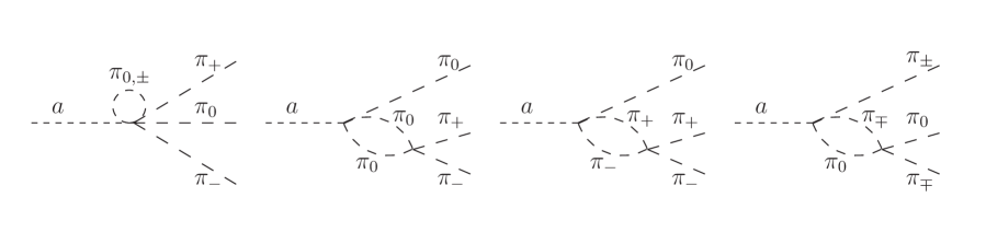
Figure 1: One-loop diagrams contributing to the ALP decay $a\to\pi_{0}\pi_{+}\pi_{-}$.

To compute the ALP decay into three pions at NLO we employ the Lehmann-Symanzik-Zimmermann (LSZ) formalism [51], according to which the amplitude is given by

$$\mathcal{M}_{a\to\pi_{0}\pi_{i}\pi_{j}}=\frac{1}{\sqrt{Z_{a}Z_{\pi}^{3}}}\Pi_{\alpha=1}^{4}\lim_{p_{\alpha}^{2}\to m_{\alpha}^{2}}\left(p_{\alpha}^{2}-m_{\alpha}^{2}\right)\times G_{a\to\pi_{0}\pi_{i}\pi_{j}}(p_{1},p_{2},p_{3},p_{4})\,,$$ (3.5)

where the index $\alpha$ runs over the external particles, $(i,j)=(+,-)$ or $(0,0)$, and $Z_{a}$ ($Z_{\pi}$) is the wave-function renormalization of the axion (pion) field defined via the residue of the 2-point Green’s functions

$$G_{\alpha\alpha}(p_{\alpha}^{2}\simeq m_{\alpha}^{2})=\frac{iZ_{\alpha}}{p_{\alpha}^{2}-m_{\alpha}^{2}}\,,$$ (3.6)

while the full 4-point Green’s function is given by

$$G_{a\to\pi_{0}\pi_{i}\pi_{j}}=\sum_{k=a,\pi_{0}}{\cal G}_{k\to\pi_{0}\pi_{i}\pi_{j}}\times G_{ak}(m^{2}_{a}=0)G_{\pi_{i}\pi_{i}}(m^{2}_{\pi})G_{\pi_{j}\pi_{j}}(m^{2}_{\pi})G_{\pi_{0}\pi_{0}}(m^{2}_{\pi})\,.$$ (3.7)

The first term is the amputated 4-point function, multiplied by the 2-point functions of the external legs with the axion mass set to zero. We work in a basis where the $a$-$\pi_{0}$ mixing has been diagonalized at the lowest-order, $\mathcal{O}(p^{2})$, via Eqs. (2.20)–(2.21) and the remaining mixing, of $\mathcal{O}(p^{4})$, is retained explicitly.

Working with LO diagonal propagators, the 2-point amplitude for the $a\text{-}\pi_{0}$ system reads

$${\cal P}_{ij}=\mbox{diag}(p^{2},p^{2}-m^{2}_{\pi})-\Sigma_{ij}\,,$$ (3.8)

where $\Sigma_{ij}$ encodes NLO corrections including mixings. The 2-point Green’s function is hence

$$G_{ij}=(-i{\cal P})^{-1}_{ij}=i\begin{pmatrix}\frac{1}{p^{2}}&\frac{\Sigma_{a\pi}}{p^{2}\left(p^{2}-m_{\pi}^{2}-\Sigma_{\pi\pi}\right)}\\ \frac{\Sigma_{a\pi}}{p^{2}\left(p^{2}-m_{\pi}^{2}-\Sigma_{\pi\pi}\right)}&\frac{1}{p^{2}-m_{\pi}^{2}-\Sigma_{\pi\pi}}\end{pmatrix}\,.$$ (3.9)

Expanding the diagonal terms around the physical masses we get (see Eq. (B.7))

$$Z_{a}=1\qquad Z_{\pi}=1+\Sigma^{\prime}_{\pi\pi}(m_{\pi}^{2})\,,$$ (3.10)

with primes indicating derivatives with respect to $p^{2}$. Then, by plugging Eq. (3.7) and (3.9) into the LSZ formula for the scattering amplitude and neglecting $\mathcal{O}(1/f_{a}^{2})$ terms, we obtain the ALP-decay amplitudes which are given by

$${\cal M}_{a\to\pi_{0}\pi_{i}\pi_{j}}=\left(1+\frac{3}{2}\Sigma^{\prime}_{\pi\pi}\right){\cal G}_{a\to\pi_{0}\pi_{i}\pi_{j}}^{\rm LO}+\frac{\Sigma_{a\pi}(p^{2}=m_{a}^{2})}{m_{a}^{2}-m_{\pi}^{2}}{\cal G}_{\pi_{0}\to\pi_{0}\pi_{i}\pi_{j}}^{\rm LO}+{\cal G}_{a\to\pi_{0}\pi_{i}\pi_{j}}^{\rm NLO}\,.$$ (3.11)

Defining the invariant mass of the two-pions systems $\pi_{\alpha}$-$\pi_{\beta}$ as $(p_{\pi_{\alpha}}+p_{\pi_{\beta}})^{2}=m_{\alpha\beta}^{2}\equiv s,t,u$ with, respectively, $(\alpha,\beta)=(+,-),(0,+),(0,-)$, we obtain

$${\cal G}_{a\to\pi_{0}\pi_{+}\pi_{-}}^{\rm LO}= \frac{3C_{a\pi}m_{\pi}^{2}\left(m_{\pi}^{2}-s\right)}{2f_{\pi}f_{a}\left(m_{a}^{2}-m_{\pi}^{2}\right)}\,,$$ (3.12)

$${\cal G}_{\pi_{0}\to\pi_{0}\pi_{+}\pi_{-}}^{\rm LO}= \frac{m_{a}^{2}+2m_{\pi}^{2}-3s}{3f_{\pi}^{2}}\,,$$ (3.13)

$${\cal G}_{a\to\pi_{0}\pi_{0}\pi_{0}}^{\rm LO}= -\frac{3m_{\pi}^{2}m_{a}^{2}C_{a\pi}}{2f_{\pi}f_{a}\left(m_{a}^{2}-m_{\pi}^{2}\right)}\,,$$ (3.14)

$${\cal G}_{\pi_{0}\to\pi_{0}\pi_{0}\pi_{0}}^{\rm LO}= -\frac{m_{\pi}^{2}}{f_{\pi}^{2}}\,,$$ (3.15)

$$\Sigma^{\prime}_{\pi\pi}= \frac{2I}{3f_{\pi}^{2}}\,,$$ (3.16)

$$\Sigma_{a\pi}(p^{2})= \frac{C_{a\pi}}{f_{\pi}f_{a}}\Bigg{(}\frac{3\ell_{3}m_{\pi}^{4}m_{a}^{2}}{m_{a}^{2}-m_{\pi}^{2}}+\frac{3\ell_{4}m_{\pi}^{2}p^{2}}{2}-\frac{I\left(4p^{2}\left(m_{a}^{2}-2m_{\pi}^{2}\right)+m_{\pi}^{2}m_{a}^{2}\right)}{4\left(m_{a}^{2}-m_{\pi}^{2}\right)}$$

$$-\frac{3\ell_{7}m_{\pi}^{4}\left(m_{a}^{2}\left(m_{d}^{2}+m_{u}^{2}-6m_{d}m_{u}\right)+4m_{\pi}^{2}m_{d}m_{u}\right)}{\left(m_{a}^{2}-m_{\pi}^{2}\right)\left(m_{d}+m_{u}\right){}^{2}}\Bigg{)}\,,$$ (3.17)

with $I$ defined in Eq. (B.4). The one-loop diagrams entering the Green’s function ${\cal G}_{a\to\pi_{0}\pi_{+}\pi_{-}}^{\rm NLO}$ are shown in Fig. 1, and the full NLO decay amplitudes are reported in Eqs. (C)–(C).

To carry out the renormalization procedure in dimensional regularization we shift the LECs as in Eq. (B.8) and we fix $\gamma_{1}=1/3$, $\gamma_{2}=2/3$, $\gamma_{3}=-1/2$, $\gamma_{4}=2$ and $\gamma_{7}=0$, consistently with the values found in the literature for the standard chiral theory [46].

3.2.1 ALP decay rate: LO vs. NLO

At LO we reproduce the decay rates given in Refs. [39, 40], that in our notation read

$$\Gamma_{a\to\pi_{i}\pi_{j}\pi_{0}}^{\text{LO}}=\frac{3C_{a\pi}^{2}}{4096\pi^{3}}\,\frac{m_{a}m_{\pi}^{4}}{f_{\pi}^{2}f_{a}^{2}}\,g^{\text{LO}}_{ij0}(m_{a})\,,$$ (3.18)

with the numerical functions $g^{\text{LO}}_{ij0}(m_{a})$ shown in the left panel of Fig. 2. Note that the $g^{\text{LO}}_{000}(m_{a})$ function includes the symmetry factor $1/6$.

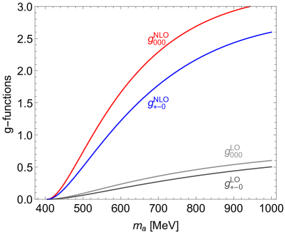
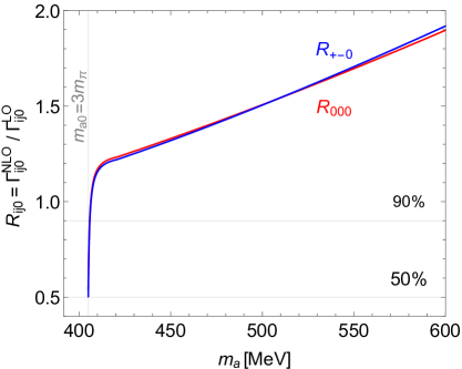
Figure 2: Left panel: Numerical profile of $g^{\text{NLO}}_{000}$ and $g^{\text{NLO}}_{+-0}$, in red and blue respectively, compared to their LO counterparts in light and dark grey. Right panel: Ratio of the NLO to LO rates for the two possible decay channels. The vertical grey line indicates the kinematical threshold for the $a\to\pi\pi\pi$ decay, with $m_{\pi}=137$ MeV corresponding to the average neutral/charged pion mass (at leading order in the isospin breaking).

At NLO we only need to consider the interference between LO and NLO amplitudes, since NLO² terms are formally of higher order. For the numerical evaluation we used the central values of the LECs $\overline{\ell_{1}}=-0.36(59)$ [52], $\overline{\ell_{2}}=4.31(11)$ [52], $\overline{\ell_{3}}=3.53(26)$ [53], $\overline{\ell_{4}}=4.73(10)$ [53] and $\ell_{7}=2.5(1.4)\times 10^{-3}$ [54], $m_{u}/m_{d}=0.50(2)$ [53], $f_{\pi}=92.1(8)$ MeV [50] and $m_{\pi}=137$ MeV (corresponding to the average neutral/charged pion mass). Then the LO+NLO rates can be written as

$$\Gamma_{a\to\pi_{i}\pi_{j}\pi_{0}}^{\text{LO+NLO}}=\frac{3C_{a\pi}^{2}}{4096\pi^{3}}\,\frac{m_{a}m_{\pi}^{4}}{f_{\pi}^{2}f_{a}^{2}}\,\left[g^{\text{LO}}_{ij0}(m_{a})+\frac{1}{16\pi^{2}}\frac{m_{a}^{2}}{f_{\pi}^{2}}g^{\text{NLO}}_{ij0}(m_{a})\right]\,,$$ (3.19)

where the NLO functions $g^{\text{LO}}_{ij0}$ are obtained by numerically integrating the NLO amplitudes in Eqs. (C)–(C). Their profile is shown in the left panel of Fig. 2, for comparison with the LO counterparts. Although the expansion parameter in Eq. (3.19) is formally written as $(m_{a}/4\pi f_{\pi})^{2}$, the actual calculation of the NLO rate shows (cf. right panel of Fig. 2) that the NLO correction becomes of the same order of the LO result already for ALP masses just above the kinematical threshold $m_{a}\gtrsim 3m_{\pi}$. This is reflected by a somewhat larger value of the NLO $g$-functions compared to the LO ones, as shown in Fig. 2.

Thus we conclude the $\chi$PT description of the $a\to\pi\pi\pi$ decay rate breaks down for ALP masses much smaller than $4\pi f_{\pi}\simeq 1.2$ GeV. This earlier breakdown of $\chi$PT is also found in SM processes that are similar to the ALP decay into pions considered here, as e.g. $\eta\to\pi\pi\pi$ (see e.g. [55, 56]). For instance, the NLO (NNLO) rate for $\eta\to\pi\pi\pi$ was found to be a factor $\approx 2.7$ $(4.5)$ larger than the LO one [55].

4 Conclusions

In this paper we have discussed the formulation of the axion-pion Lagrangian at the NLO in $\chi$PT and considered as an application of phenomenological relevance the ALP decay $a\to\pi\pi\pi$, which is one of the main hadronic channels for GeV-scale ALPs. Through the inclusion of the NLO correction, we have estimated the range of applicability of the chiral expansion and found that the chiral EFT fails for ALP masses just above the kinematical threshold of $3m_{\pi}$ (cf. right panel in Fig. 2). This result shows an earlier breakdown of the chiral EFT compared to naive expectations based on previous LO calculations, see Refs. [39, 40]. We conclude that the range of applicability of the axion-pion chiral Lagrangian is rather limited for the problem at hand (similar conclusions were achieved for the case of $a\pi\to\pi\pi$ scattering in Ref. [26]) and hence alternative non-perturbative approaches (based either on dispersion relations or lattice QCD techniques) are called for in order to extend the validity of the chiral description.

Appendix A Pion axial current

In this Appendix we provide the derivation of the pion axial current at the NLO. The currents associated to the Left and Right chiral rotations

$$L=\exp\left(-i\Theta_{L}^{a}\frac{\sigma^{a}}{2}\right)\,,\qquad R=\exp\left(-i\Theta_{R}^{a}\frac{\sigma^{a}}{2}\right)\,,$$ (A.1)

acting on the Goldstone matrix as $U\to RUL^{\dagger}$, are easily computed promoting the global symmetries to local ones, and computing the variation $\delta\mathcal{L}$ of the Lagrangian under the given transformation. From Noether’s theorem, the Left and Right currents are given by

$$J_{L,R}^{\mu,a}=-\frac{\partial\delta\mathcal{L}}{\partial\partial_{\mu}\Theta^{a}_{L,R}(x)}\,.$$ (A.2)

Let us consider the LO chiral Lagrangian

$$\mathcal{L}_{\chi}=\frac{f_{\pi}^{2}}{4}{\rm Tr}\left[\partial^{\mu}U^{\dagger}\partial_{\mu}U+U\chi^{\dagger}+\chi U^{\dagger}\right]\,.$$ (A.3)

To compute e.g. the Right current, we set $\Theta^{a}_{L}(x)=0$ and perform an infinitesimal Right transformation

$$U\rightarrow\left(1-i\Theta^{a}_{R}(x)\frac{\sigma^{a}}{2}\right)U\,.$$ (A.4)

The variation of $\mathcal{L}_{\chi}$ is

$$\delta\mathcal{L}_{\chi}=\frac{i}{4}f_{\pi}^{2}\partial_{\mu}\Theta^{a}_{R}(x){\rm Tr}\left[\partial^{\mu}UU^{\dagger}\sigma^{a}\right]\,,$$ (A.5)

and therefore $J_{R}^{\mu,a}$ is given by

$$J_{R}^{\mu,a}=-\frac{i}{4}f_{\pi}^{2}{\rm Tr}\left[\partial^{\mu}UU^{\dagger}\sigma^{a}\right]\,.$$ (A.6)

With an analogous procedure one obtains

$$J_{L}^{\mu,a}=-\frac{i}{4}f_{\pi}^{2}{\rm Tr}\left[\partial^{\mu}U^{\dagger}U\sigma^{a}\right]\,.$$ (A.7)

The $R-L$ combination of these two currents provides the pion axial current at LO

$$J_{A}^{\mu,a}=\frac{i}{4}f_{\pi}^{2}{\rm Tr}\left[\sigma^{a}\{U,\partial^{\mu}U^{\dagger}\}\right]\,.$$ (A.8)

The procedure can be repeated at the NLO by employing the shift of the $\mathcal{O}(p^{4})$ chiral Lagrangian in Eq. (2.3), which yields

$$J_{R\ (\rm NLO)}^{\mu,a}=+i \frac{\ell_{1}}{2}\mbox{Tr}\left[\sigma^{a}UD^{\mu}U^{\dagger}\right]\mbox{Tr}\left[D_{\nu}UD^{\nu}U^{\dagger}\right]$$ (A.9)

$$+i \frac{\ell_{2}}{4}\mbox{Tr}\left[\sigma^{a}UD^{\nu}U^{\dagger}\right]\mbox{Tr}\left[D^{\mu}UD_{\nu}U^{\dagger}+D_{\nu}UD^{\mu}U^{\dagger}\right]$$

$$+i \frac{\ell_{4}}{8}\mbox{Tr}\left[\sigma^{a}D^{\mu}U\chi^{\dagger}-\sigma^{a}UD^{\mu}\chi^{\dagger}+\sigma^{a}D^{\mu}\chi U^{\dagger}-\sigma^{a}\chi D^{\mu}U^{\dagger}\right]$$

$$+ \frac{\ell_{6}}{4}\mbox{Tr}\left[f_{\mu\nu}^{R}\left(\sigma^{a}D^{\nu}UU^{\dagger}+UD^{\nu}U^{\dagger}\sigma^{a}\right)+f_{\mu\nu}^{L}\left(U^{\dagger}\sigma^{a}D^{\nu}U+D^{\nu}U^{\dagger}\sigma^{a}U\right)\right]\,,$$

and

$$J_{L\ (\rm NLO)}^{\mu,a}=-i \frac{\ell_{1}}{2}\mbox{Tr}\left[\sigma^{a}D^{\mu}U^{\dagger}U\right]\mbox{Tr}\left[D_{\nu}UD^{\nu}U^{\dagger}\right]$$ (A.10)

$$-i \frac{\ell_{2}}{4}\mbox{Tr}\left[\sigma^{a}D^{\nu}U^{\dagger}U\right]\mbox{Tr}\left[D_{\nu}UD_{\mu}U^{\dagger}+D_{\mu}UD_{\nu}U^{\dagger}\right]$$

$$-i \frac{\ell_{4}}{8}\mbox{Tr}\left[\sigma^{a}\chi^{\dagger}D^{\mu}U-\sigma^{a}D^{\mu}\chi^{\dagger}U+\sigma^{a}U^{\dagger}D^{\mu}\chi-\sigma^{a}D^{\mu}U^{\dagger}\chi\right]$$

$$+ \frac{\ell_{6}}{4}\mbox{Tr}\left[f_{\mu\nu}^{R}\left(D^{\nu}U\sigma^{a}U^{\dagger}+U\sigma^{a}D^{\nu}U^{\dagger}\right)+f_{\mu\nu}^{L}\left(U^{\dagger}D^{\nu}U\sigma^{a}+\sigma^{a}D^{\nu}U^{\dagger}U\right)\right]\,.$$

Combining the left and right currents we obtain the axial current in Eq. (2.25).

Appendix B Axion-pion mixing at NLO

We explicitly perform here the NLO diagonalization of the axion and neutral pion propagators. The axion-neutral pion Lagrangian up to order $1/f_{a}$ is given by

$$\mathcal{L}_{\text{$a$-$\pi_{0}$}}=\frac{1}{2}\left(\partial_{\mu}a\right)^{2}+\frac{1}{2}\left(\partial_{\mu}\pi_{0b}\right)^{2}-\frac{1}{2}m_{a}^{2}a^{2}-\frac{1}{2}m_{\pi}^{2}\pi_{0b}^{2}+\mathcal{L}_{\rm int}$$ (B.1)

where the subscript $b$ stands for bare fields and the interaction Lagrangian reads explicitly

$$\mathcal{L}_{\rm int} =-a\pi_{0b}\ \ell_{7}\frac{4m_{d}m_{u}m_{\pi}^{4}\left(m_{d}-m_{u}\right)}{f_{a}f_{\pi}\left(m_{d}+m_{u}\right){}^{3}}-\frac{3C_{a\pi}}{2f_{a}}\partial_{\mu}a\partial^{\mu}\pi_{0b}\left(f_{\pi}+\ell_{4}\frac{m_{\pi}^{2}}{f_{\pi}}\right)$$

$$+ \frac{2C_{a\pi}}{f_{a}f_{\pi}}\partial_{\mu}a\ \partial^{\mu}\pi_{0b}\ \pi_{+}\ \pi_{-}+\frac{1}{24f_{\pi}^{2}}m_{\pi}^{2}\pi_{0b}^{4}-\frac{1}{3f_{\pi}^{2}}\pi_{0b}^{2}\partial_{\mu}\pi_{+}\partial^{\mu}\pi_{-}$$

$$+ \frac{1}{6f_{\pi}^{2}}m_{\pi}^{2}\pi_{+}\pi_{-}\pi_{0b}^{2}-\frac{1}{3f_{\pi}^{2}}\pi_{+}\pi_{-}\partial_{\mu}\pi_{0b}\partial^{\mu}\pi_{0b}-\frac{\ell_{3}m_{\pi}^{4}\pi_{0b}^{2}}{f_{\pi}^{2}}+\frac{\ell_{7}\pi_{0b}^{2}(m_{d}-m_{u})^{2}m_{\pi}^{4}}{f_{\pi}^{2}(m_{u}+m_{d})^{2}}\,.$$ (B.2)

Note that $\mathcal{L}_{\rm int}$ contains all the terms which contribute to the two-point functions of the neutral scalar fields, i.e. LO tree-level mixings, LO terms giving the one-loop corrections and NLO terms. The latter provide the counterterms needed to reabsorb the loop divergences.

We next define the renormalization conditions. Firstly, it is important to note that, since the divergences come from loops of $\mathcal{L}^{\chi({\rm LO})}_{a}$, it is sufficient to extract the counterterms from $\ell_{3}$, $\ell_{4}$ and $\ell_{7}$. Hence, $m_{\pi}$ and $f_{\pi}$ are the physical pion mass and decay constant at LO. Let us now denote by $-i\Sigma_{ij}(p^{2})$ (with $i,j=a,\pi_{0}$) the 1-particle-irreducible (1PI) self-energy correction. The net effect of this correction is encoded in the effective Lagrangian

$$\begin{split}\mathcal{L}_{\text{$a$-$\pi_{0}$}}^{\rm eff}=&\frac{1}{2}a\left(p^{2}-m_{a}^{2}\right)a+\frac{1}{2}\pi_{0}\left(p^{2}-m_{\pi}^{2}+(p^{2}-m_{\pi}^{2})\delta Z_{\pi}-\Sigma_{\pi\pi}(p^{2})\right)\pi_{0}\\ -&a\Sigma_{a\pi}(p^{2})\left(1+\frac{1}{2}\delta Z_{\pi}\right)\pi_{0}\,,\end{split}$$ (B.3)

where we employed the pion wave-function renormalization, $\pi_{0b}\rightarrow(1+\frac{1}{2}\delta Z_{\pi})\pi_{0}$, defined as $\delta Z_{\pi}=\partial\Sigma_{\pi\pi}(p^{2})/\partial p^{2}$. The one-loop self-energies $\Sigma_{ij}(p^{2})$ can be computed from the interaction Lagrangian in Eq. (B). Defining

$$I=\frac{m_{\pi}^{2}}{16\pi^{2}}\left[R+\log\left(\frac{m_{\pi}^{2}}{\mu^{2}}\right)\right],\\$$ (B.4)

with $R=\frac{2}{d-4}-\log(4\pi)+\gamma_{E}-1$, and using dimensional regularization we find

$$\Sigma_{\pi\pi}(p^{2}) =I\frac{1}{6f_{\pi}^{2}}[4p^{2}-m_{\pi}^{2}]+\frac{2\ell_{3}m_{\pi}^{4}}{f_{\pi}^{2}}-\frac{2\ell_{7}(m_{d}-m_{u})^{2}m_{\pi}^{4}}{f_{\pi}^{2}(m_{u}+m_{d})^{2}}\,,$$ (B.5)

$$\Sigma_{a\pi}(p^{2}) =3C_{a\pi}p^{2}\left[\frac{f_{\pi}}{2f_{a}}+\frac{\ell_{4}m_{\pi}^{2}}{2f_{a}f_{\pi}}-\frac{2I}{3f_{a}f_{\pi}}\right]+\frac{4\ell_{7}(m_{d}-m_{u})m_{u}m_{d}m_{\pi}^{4}}{f_{a}f_{\pi}(m_{u}+m_{d})^{3}}\,,$$ (B.6)

from which we get

$$\delta Z_{\pi}=\frac{2I}{3f_{\pi}^{2}}\,.$$ (B.7)

Therefore, we define the scale-independent parameters $\overline{\ell_{i}}$ and $\overline{h_{i}}$ in such a way that the $R+\log(m_{\pi}^{2}/\mu^{2})$ factor is subtracted [46]

$$\begin{split}\ell_{i}=&\frac{\gamma_{i}}{32\pi^{2}}\left[\overline{\ell_{i}}+R+\log\left(\frac{m_{\pi}^{2}}{\mu^{2}}\right)\right]\,,\\ h_{i}=&\frac{\delta_{i}}{32\pi^{2}}\left[\overline{h}_{i}+R+\log\left(\frac{m_{\pi}^{2}}{\mu^{2}}\right)\right]\,.\end{split}$$ (B.8)

Plugging these definitions in Eqs. (B.5)–(B.6) and substituting back into Eq. (B.3) we find that in order to renormalize $\Sigma_{\pi\pi}$ and $\Sigma_{a\pi}$ we need to set

$$\gamma_{3}=-\frac{1}{2}\,,\qquad\gamma_{4}=2\,.$$ (B.9)

Thus the renormalized effective Lagrangian becomes

$$\mathcal{L}_{a-\pi_{0}}^{\rm eff}=\frac{1}{2}a\left(p^{2}-m_{a}^{2}\right)a+\frac{1}{2}\pi_{0}\left(p^{2}-\widetilde{m}_{\pi}^{2}\right)\pi_{0}-a\left(p^{2}3C_{a\pi}\frac{\tilde{f_{\pi}}}{2f_{a}}+\frac{4\ell_{7}(m_{d}-m_{u})m_{u}m_{d}m_{\pi}^{4}}{f_{a}f_{\pi}(m_{u}+m_{d})^{3}}\right)\pi_{0}\,,$$ (B.10)

with

$$\widetilde{m}_{\pi}^{2}=m_{\pi}^{2}-\frac{m_{\pi}^{4}\overline{\ell_{3}}}{32\pi^{2}f_{\pi}^{2}}-\frac{2\ell_{7}(m_{d}-m_{u})^{2}m_{\pi}^{4}}{f_{\pi}^{2}(m_{u}+m_{d})^{2}}\,,$$ (B.11)

and

$$\tilde{f}_{\pi}=f_{\pi}+\frac{\overline{\ell_{4}}m_{\pi}^{2}}{16\pi^{2}f_{\pi}}\,.$$ (B.12)

We observe that $\ell_{7}$ is not renormalized, since in the LO Lagrangian the $m_{d}-m_{u}$ terms are all momentum dependent. So we are left with a non-zero off-diagonal two-point function. In order to eliminate the mixing, we can rotate the axion and the pion fields as

$$\begin{split}a&\rightarrow a-\beta_{1}\pi_{0}\,,\\ \pi_{0}&\rightarrow\pi_{0}-\beta_{2}a\,,\end{split}$$ (B.13)

yielding

$$\begin{split}\mathcal{L}_{a-\pi_{0}}^{\rm eff}\rightarrow&\ \frac{1}{2}a\left(p^{2}-m_{a}^{2}\right)a+\frac{1}{2}\pi_{0}\left(p^{2}-\tilde{m}_{\pi}^{2}\right)\pi_{0}\\ &-a\left(\beta_{1}(p^{2}-m_{a}^{2})+\beta_{2}(p^{2}-m_{\pi}^{2})+p^{2}3C_{a\pi}\frac{\tilde{f_{\pi}}}{2f_{a}}+\frac{4\ell_{7}(m_{d}-m_{u})m_{u}m_{d}m_{\pi}^{4}}{f_{a}f_{\pi}(m_{u}+m_{d})^{3}}\right)\pi_{0}\,.\end{split}$$ (B.14)

Hence, to cancel the mixing term it is sufficient to set

$$\beta_{1} =-3C_{a\pi}\frac{\tilde{f_{\pi}}}{2f_{a}}-\left(m_{\pi}^{2}-m_{a}^{2}\right)^{-1}\left[3C_{a\pi}\frac{\tilde{f_{\pi}}}{2f_{a}}m_{a}^{2}+\frac{4\ell_{7}(m_{d}-m_{u})m_{u}m_{d}m_{\pi}^{4}}{f_{a}f_{\pi}(m_{u}+m_{d})^{3}}\right]\,,$$ (B.15)

$$\beta_{2} =\left(m_{\pi}^{2}-m_{a}^{2}\right)^{-1}\left[3C_{a\pi}\frac{\tilde{f_{\pi}}}{2f_{a}}m_{a}^{2}+\frac{4\ell_{7}(m_{d}-m_{u})m_{u}m_{d}m_{\pi}^{4}}{f_{a}f_{\pi}(m_{u}+m_{d})^{3}}\right]\,.$$ (B.16)

Appendix C ALP decay amplitudes

Following Eq. (3.11), the full ALP decay amplitudes up to NLO are given by (employing the definition $\sigma(x)=(1-4m_{\pi}^{2}/x)^{1/2}$)

$${\cal M}_{a\to\pi_{0}\pi_{+}\pi_{-}}=\frac{3C_{a\pi}m_{\pi}^{2}\left(m_{\pi}^{2}-s\right)}{2f_{a}f_{\pi}\left(m_{a}^{2}-m_{\pi}^{2}\right)}$$

$$+\frac{C_{a\pi}}{32\pi^{2}f_{a}f_{\pi}^{3}\left(m_{a}^{2}-m_{\pi}^{2}\right)}\Bigg{\{}\overline{\ell_{1}}m_{\pi}^{2}\left(2m_{\pi}^{2}-s\right)\left(m_{a}^{2}+m_{\pi}^{2}-s\right)$$

$$+\overline{\ell_{2}}m_{\pi}^{2}\left(m_{a}^{2}\left(2m_{\pi}^{2}-s\right)+m_{a}^{4}-3m_{\pi}^{2}s+5m_{\pi}^{4}-u^{2}-t^{2}\right)$$

$$+\frac{3}{2}\overline{\ell_{3}}m_{\pi}^{4}\frac{m_{a}^{4}-m_{\pi}^{2}(m_{a}^{2}+m_{\pi}^{2}-s)}{m_{a}^{2}-m_{\pi}^{2}}+3\overline{\ell_{4}}m_{\pi}^{2}\left(m_{a}^{2}+m_{\pi}^{2}\right)\left(m_{\pi}^{2}-s\right)$$

$$+\frac{1}{6}m_{\pi}^{2}(m_{a}^{2}\left(45m_{\pi}^{2}-29s\right)+11m_{a}^{4}-15m_{\pi}^{2}s+45m_{\pi}^{4}-11t^{2}-8tu-11u^{2})$$

$$-\frac{1}{2}\log\left(\frac{\sigma(u)-1}{\sigma(u)+1}\right)\sigma(u)\Big{(}3m_{\pi}^{4}+(u-4t)m_{\pi}^{2}$$

$$+(t-u)u+m_{a}^{2}\left(u-m_{\pi}^{2}\right)\Big{)}m_{\pi}^{2}$$

$$-\frac{1}{2}\log\left(\frac{\sigma(t)-1}{\sigma(t)+1}\right)\sigma(t)\Big{(}3m_{\pi}^{4}+(t-4u)m_{\pi}^{2}$$

$$+(u-t)t+m_{a}^{2}\left(t-m_{\pi}^{2}\right)\Big{)}m_{\pi}^{2}$$

$$+\frac{3}{2}\log\left(\frac{\sigma(s)-1}{\sigma(s)+1}\right)\sigma(s)\left(m_{\pi}^{2}-s\right)\left(m_{a}^{2}+s\right)m_{\pi}^{2}\Bigg{\}}$$

$$+\ell_{7}\frac{\left(m_{d}-m_{u}\right)m_{\pi}^{4}}{3f_{a}f_{\pi}^{3}(m_{a}^{2}-m_{\pi}^{2})^{2}\left(m_{d}+m_{u}\right)^{3}}\Big{[}\Big{(}m_{a}^{2}\left(3s(m_{d}^{2}+m_{u}^{2}-6m_{d}m_{u})-4m_{\pi}^{2}\left(m_{d}^{2}-11m_{d}m_{u}+m_{u}^{2}\right)\right)$$

$$+m_{a}^{4}\left(m_{d}^{2}-14m_{d}m_{u}+m_{u}^{2}\right)-12m_{d}m_{\pi}^{2}m_{u}\left(2m_{\pi}^{2}-s\right)\Big{)}\Big{]}\,,$$ (C.1)

and

$${\cal M}_{a\to\pi_{0}\pi_{0}\pi_{0}}=-\frac{3C_{a\pi}m_{\pi}^{2}m_{{a}}^{2}}{2f_{\pi}f_{a}\left(m_{{a}}^{2}-m_{\pi}^{2}\right)}$$

$$+\frac{C_{a\pi}}{32\pi^{2}f_{a}f_{\pi}^{3}\left(m_{a}^{2}-m_{\pi}^{2}\right)}\Bigg{\{}2\overline{\ell_{1}}m_{\pi}^{2}\left(m_{a}^{2}\left(3m_{\pi}^{2}-s\right)+m_{a}^{4}-3m_{\pi}^{2}s+6m_{\pi}^{4}-t^{2}-tu-u^{2}\right)$$

$$+4\overline{\ell_{2}}m_{\pi}^{2}\left(m_{a}^{2}\left(3m_{\pi}^{2}-s\right)+m_{a}^{4}-3m_{\pi}^{2}s+6m_{\pi}^{4}-t^{2}-tu-u^{2}\right)$$

$$+\frac{3}{2}\overline{\ell_{3}}m_{a}^{2}m_{\pi}^{4}\frac{3m_{a}^{2}-2m_{\pi}^{2}}{m_{a}^{2}-m_{\pi}^{2}}-3\overline{\ell_{4}}m_{a}^{2}m_{\pi}^{2}\left(m_{a}^{2}+m_{\pi}^{2}\right)$$

$$+\frac{3}{2}\log\left(\frac{\sigma(s)-1}{\sigma(s)+1}\right)m_{\pi}^{2}\sigma(s)\left(m_{\pi}^{2}m_{{a}}^{2}+2\left(m_{\pi}^{2}-s\right)^{2}\right)$$

$$+\frac{3}{2}\log\left(\frac{\sigma(t)-1}{\sigma(t)+1}\right)m_{\pi}^{2}\sigma(t)\left(m_{\pi}^{2}m_{{a}}^{2}+2\left(m_{\pi}^{2}-t\right)^{2}\right)$$

$$+\frac{3}{2}\log\left(\frac{\sigma(u)-1}{\sigma(u)+1}\right)m_{\pi}^{2}\sigma(u)\left(m_{\pi}^{2}m_{{a}}^{2}+2\left(m_{\pi}^{2}-u\right)^{2}\right)$$

$$+\frac{3}{2}m_{\pi}^{2}\left(-4s\left(m_{a}^{2}+3m_{\pi}^{2}\right)+13m_{a}^{2}m_{\pi}^{2}+2m_{a}^{4}+24m_{\pi}^{4}-4\left(t^{2}+tu+u^{2}\right)\right)\Bigg{\}}$$

$$+\frac{\ell_{7}m_{\pi}^{4}\left(4m_{a}^{2}-3m_{\pi}^{2}\right)(m_{d}-m_{u})\left(m_{a}^{2}(m_{d}^{2}+m_{u}^{2}-6m_{d}m_{u})+4m_{d}m_{\pi}^{2}m_{u}\right)}{f_{a}f_{\pi}^{3}\left(m_{a}^{2}-m_{\pi}^{2}\right)^{2}(m_{d}+m_{u})^{3}}\,.$$ (C.2)

References

- [1] R. D. Peccei and H. R. Quinn, “CP Conservation in the Presence of Instantons,” Phys. Rev. Lett. 38 (1977) 1440–1443.
- [2] R. D. Peccei and H. R. Quinn, “Constraints Imposed by CP Conservation in the Presence of Instantons,” Phys. Rev. D16 (1977) 1791–1797.
- [3] S. Weinberg, “A New Light Boson?,” Phys. Rev. Lett. 40 (1978) 223–226.
- [4] F. Wilczek, “Problem of Strong p and t Invariance in the Presence of Instantons,” Phys. Rev. Lett. 40 (1978) 279–282.
- [5] W. A. Bardeen and S. H. H. Tye, “Current Algebra Applied to Properties of the Light Higgs Boson,” Phys. Lett. B 74 (1978) 229–232.
- [6] P. Di Vecchia and G. Veneziano, “Chiral Dynamics in the Large n Limit,” Nucl. Phys. B 171 (1980) 253–272.
- [7] D. B. Kaplan, “Opening the Axion Window,” Nucl. Phys. B 260 (1985) 215–226.
- [8] M. Srednicki, “Axion Couplings to Matter. 1. CP Conserving Parts,” Nucl. Phys. B260 (1985) 689–700.
- [9] H. Georgi, D. B. Kaplan, and L. Randall, “Manifesting the Invisible Axion at Low-energies,” Phys. Lett. B 169 (1986) 73–78.
- [10] M. Spalinski, “Chiral Corrections to the Axion Mass,” Z. Phys. C 41 (1988) 87–90.
- [11] TWQCD Collaboration, Y.-Y. Mao and T.-W. Chiu, “Topological Susceptibility to the One-Loop Order in Chiral Perturbation Theory,” Phys. Rev. D 80 (2009) 034502, arXiv:0903.2146 [hep-lat].
- [12] G. Grilli di Cortona, E. Hardy, J. Pardo Vega, and G. Villadoro, “The QCD axion, precisely,” JHEP 01 (2016) 034, arXiv:1511.02867 [hep-ph].
- [13] I. G. Irastorza and J. Redondo, “New experimental approaches in the search for axion-like particles,” Prog. Part. Nucl. Phys. 102 (2018) 89–159, arXiv:1801.08127 [hep-ph].
- [14] P. Sikivie, “Invisible Axion Search Methods,” Rev. Mod. Phys. 93 no. 1, (2021) 015004, arXiv:2003.02206 [hep-ph].
- [15] M. Gorghetto and G. Villadoro, “Topological Susceptibility and QCD Axion Mass: QED and NNLO corrections,” JHEP 03 (2019) 033, arXiv:1812.01008 [hep-ph].
- [16] S. Borsanyi et al., “Calculation of the axion mass based on high-temperature lattice quantum chromodynamics,” Nature 539 no. 7627, (2016) 69–71, arXiv:1606.07494 [hep-lat].
- [17] T. Vonk, F.-K. Guo, and U.-G. Meißner, “Precision calculation of the axion-nucleon coupling in chiral perturbation theory,” JHEP 03 (2020) 138, arXiv:2001.05327 [hep-ph].
- [18] T. Vonk, F.-K. Guo, and U.-G. Meißner, “The axion-baryon coupling in SU(3) heavy baryon chiral perturbation theory,” JHEP 08 (2021) 024, arXiv:2104.10413 [hep-ph].
- [19] F. Bigazzi, A. L. Cotrone, M. Järvinen, and E. Kiritsis, “Non-derivative Axionic Couplings to Nucleons at large and small N,” JHEP 01 (2020) 100, arXiv:1906.12132 [hep-ph].
- [20] S. Bertolini, L. Di Luzio, and F. Nesti, “Axion-mediated forces, CP violation and left-right interactions,” Phys. Rev. Lett. 126 no. 8, (2021) 081801, arXiv:2006.12508 [hep-ph].
- [21] S. Okawa, M. Pospelov, and A. Ritz, “Long-range axion forces and hadronic CP violation,” Phys. Rev. D 105 no. 7, (2022) 075003, arXiv:2111.08040 [hep-ph].
- [22] W. Dekens, J. de Vries, and S. Shain, “CP-violating axion interactions in effective field theory,” arXiv:2203.11230 [hep-ph].
- [23] J. Martin Camalich, M. Pospelov, P. N. H. Vuong, R. Ziegler, and J. Zupan, “Quark Flavor Phenomenology of the QCD Axion,” Phys. Rev. D 102 no. 1, (2020) 015023, arXiv:2002.04623 [hep-ph].
- [24] M. Bauer, M. Neubert, S. Renner, M. Schnubel, and A. Thamm, “Consistent Treatment of Axions in the Weak Chiral Lagrangian,” Phys. Rev. Lett. 127 no. 8, (2021) 081803, arXiv:2102.13112 [hep-ph].
- [25] A. W. M. Guerrera and S. Rigolin, “Revisiting decays,” Eur. Phys. J. C 82 no. 3, (2022) 192, arXiv:2106.05910 [hep-ph].
- [26] L. Di Luzio, G. Martinelli, and G. Piazza, “Breakdown of chiral perturbation theory for the axion hot dark matter bound,” Phys. Rev. Lett. 126 no. 24, (2021) 241801, arXiv:2101.10330 [hep-ph].
- [27] S. Chang and K. Choi, “Hadronic axion window and the big bang nucleosynthesis,” Phys. Lett. B 316 (1993) 51–56, arXiv:hep-ph/9306216.
- [28] S. Hannestad, A. Mirizzi, and G. Raffelt, “New cosmological mass limit on thermal relic axions,” JCAP 07 (2005) 002, arXiv:hep-ph/0504059.
- [29] Y. Aoki, Z. Fodor, S. D. Katz, and K. K. Szabo, “The QCD transition temperature: Results with physical masses in the continuum limit,” Phys. Lett. B 643 (2006) 46–54, arXiv:hep-lat/0609068.
- [30] Wuppertal-Budapest Collaboration, S. Borsanyi, Z. Fodor, C. Hoelbling, S. D. Katz, S. Krieg, C. Ratti, and K. K. Szabo, “Is there still any mystery in lattice QCD? Results with physical masses in the continuum limit III,” JHEP 09 (2010) 073, arXiv:1005.3508 [hep-lat].
- [31] A. Bazavov et al., “The chiral and deconfinement aspects of the QCD transition,” Phys. Rev. D 85 (2012) 054503, arXiv:1111.1710 [hep-lat].
- [32] F. D’Eramo, F. Hajkarim, and S. Yun, “Thermal Axion Production at Low Temperatures: A Smooth Treatment of the QCD Phase Transition,” Phys. Rev. Lett. 128 no. 15, (2022) 152001, arXiv:2108.04259 [hep-ph].
- [33] F. D’Eramo, F. Hajkarim, and S. Yun, “Thermal QCD Axions across Thresholds,” JHEP 10 (2021) 224, arXiv:2108.05371 [hep-ph].
- [34] L. Caloni, M. Gerbino, M. Lattanzi, and L. Visinelli, “Novel cosmological bounds on thermally-produced axion-like particles,” arXiv:2205.01637 [astro-ph.CO].
- [35] F. D’Eramo, E. Di Valentino, W. Giarè, F. Hajkarim, A. Melchiorri, O. Mena, F. Renzi, and S. Yun, “Cosmological Bound on the QCD Axion Mass, Redux,” arXiv:2205.07849 [astro-ph.CO].
- [36] D. Aloni, Y. Soreq, and M. Williams, “Coupling QCD-Scale Axionlike Particles to Gluons,” Phys. Rev. Lett. 123 no. 3, (2019) 031803, arXiv:1811.03474 [hep-ph].
- [37] K. J. Kelly, S. Kumar, and Z. Liu, “Heavy axion opportunities at the DUNE near detector,” Phys. Rev. D 103 no. 9, (2021) 095002, arXiv:2011.05995 [hep-ph].
- [38] H.-C. Cheng, L. Li, and E. Salvioni, “A theory of dark pions,” JHEP 01 (2022) 122, arXiv:2110.10691 [hep-ph].
- [39] M. Bauer, M. Neubert, and A. Thamm, “Collider Probes of Axion-Like Particles,” JHEP 12 (2017) 044, arXiv:1708.00443 [hep-ph].
- [40] M. Bauer, M. Neubert, S. Renner, M. Schnubel, and A. Thamm, “The Low-Energy Effective Theory of Axions and ALPs,” JHEP 04 (2021) 063, arXiv:2012.12272 [hep-ph].
- [41] L. Di Luzio, M. Giannotti, E. Nardi, and L. Visinelli, “The landscape of QCD axion models,” Phys. Rept. 870 (2020) 1–117, arXiv:2003.01100 [hep-ph].
- [42] J. E. Kim, “Weak Interaction Singlet and Strong CP Invariance,” Phys. Rev. Lett. 43 (1979) 103.
- [43] M. A. Shifman, A. I. Vainshtein, and V. I. Zakharov, “Can Confinement Ensure Natural CP Invariance of Strong Interactions?,” Nucl. Phys. B166 (1980) 493.
- [44] A. R. Zhitnitsky, “On Possible Suppression of the Axion Hadron Interactions. (In Russian),” Sov. J. Nucl. Phys. 31 (1980) 260. [Yad. Fiz.31,497(1980)].
- [45] M. Dine, W. Fischler, and M. Srednicki, “A Simple Solution to the Strong CP Problem with a Harmless Axion,” Phys. Lett. B104 (1981) 199–202.
- [46] J. Gasser and H. Leutwyler, “Chiral Perturbation Theory to One Loop,” Annals Phys. 158 (1984) 142.
- [47] S. Scherer, “Introduction to chiral perturbation theory,” Adv. Nucl. Phys. 27 (2003) 277, arXiv:hep-ph/0210398.
- [48] J. Wess and B. Zumino, “Consequences of anomalous Ward identities,” Phys. Lett. B 37 (1971) 95–97.
- [49] E. Witten, “Global Aspects of Current Algebra,” Nucl. Phys. B 223 (1983) 422–432.
- [50] Particle Data Group Collaboration, P. Zyla et al., “Review of Particle Physics,” PTEP 2020 no. 8, (2020) 083C01.
- [51] H. Lehmann, K. Symanzik, and W. Zimmermann, “On the formulation of quantized field theories,” Nuovo Cim. 1 (1955) 205–225.
- [52] G. Colangelo, J. Gasser, and H. Leutwyler, “ scattering,” Nucl. Phys. B 603 (2001) 125–179, arXiv:hep-ph/0103088.
- [53] Flavour Lattice Averaging Group Collaboration, S. Aoki et al., “FLAG Review 2019: Flavour Lattice Averaging Group (FLAG),” Eur. Phys. J. C 80 no. 2, (2020) 113, arXiv:1902.08191 [hep-lat].
- [54] R. Frezzotti, G. Gagliardi, V. Lubicz, G. Martinelli, F. Sanfilippo, and S. Simula, “First direct lattice calculation of the chiral perturbation theory low-energy constant ,” arXiv:2107.11895 [hep-lat].
- [55] J. Bijnens and K. Ghorbani, “eta — 3 pi at Two Loops In Chiral Perturbation Theory,” JHEP 11 (2007) 030, arXiv:0709.0230 [hep-ph].
- [56] J. Bijnens and J. Gasser, “Eta decays at and beyond p**4 in chiral perturbation theory,” Phys. Scripta T 99 (2002) 34–44, arXiv:hep-ph/0202242.