pterodactyls: A Tool to Uniformly Search and Vet for Young Transiting Planets In TESS Primary Mission Photometry

Abstract

Kepler’s short-period exoplanet population has revealed evolutionary features such as the Radius Valley and the Hot Neptune desert that are likely sculpted by atmospheric loss over time. These findings suggest that the primordial planet population is different from the Gyr-old Kepler population, and motivates exoplanet searches around young stars. Here, we present pterodactyls, a data reduction pipeline specifically built to address the challenges in discovering exoplanets around young stars and to work with TESS Primary Mission 30-min cadence photometry, since most young stars were not pre-selected TESS 2-min cadence targets. pterodactyls builds on publicly available and tested tools in order to extract, detrend, search, and vet transiting young planet candidates. We search five clusters with known transiting planets: Tucana-Horologium Association, IC 2602, Upper Centaurus Lupus, Ursa Major and Pisces Eridani. We show that pterodactyls recovers seven out of the eight confirmed planets and one out of the two planet candidates, most of which were initially detected in 2-min cadence data. For these clusters, we conduct injection-recovery tests to characterize our detection efficiency, and compute an intrinsic planet occurrence rate of 49$\pm$20% for sub-Neptunes and Neptunes (1.8-6 $R_{\oplus}$) within 12.5 days, which is higher than Kepler’s Gyr-old occurrence rates of 6.8$\pm$0.3%. This potentially implies that these planets have shrunk with time due to atmospheric mass loss. However, a proper assessment of the occurrence of transiting young planets will require a larger sample unbiased to planets already detected. As such, pterodactyls will be used in future work to search and vet for planet candidates in nearby clusters and moving groups.

1 Introduction

The Kepler mission was instrumental in the discovery of thousands of exoplanets (Borucki et al., 2010; Borucki, 2017), most of which were found to be closer to their star than Mercury is to our Sun. A closer look at this population of short-period exoplanets revealed two prominent features: the Hot Neptune Desert and the Radius Valley. The Hot Neptune Desert (3$-$10 $R_{\oplus}$; $<$4 days) is a region in the Gyr-old, period-radius plane with a significant dearth of Neptune-sized planets (Beaugé & Nesvorný, 2013). As Neptune-sized planets should be easier to find in short-period orbits, and many sub-Neptunes have been discovered with longer orbital periods from surveys such as CoRoT (Baglin et al., 2006) and Kepler, the Hot Neptune Desert appears to not be an observational bias. The Radius Valley, a region with a much lower frequency of planets with radii $\sim$1.8 $R_{\oplus}$ than at $\sim$1.3 $R_{\oplus}$ (Super-Earths) or at $\sim$2.4 $R_{\oplus}$ (sub-Neptunes), was discovered by Fulton et al. (2017) using accurate stellar, and hence planetary, radii from the California-Kepler survey (Petigura et al., 2017; Johnson et al., 2017). More recently, the Radius Valley was also detected in K2 data (Hardegree-Ullman et al., 2020).

Both the Hot Neptune Desert and the Radius valley are most likely caused by atmospheric mass loss due to XUV photoevaporation (see, e.g. Owen & Wu 2013, 2017) and/or core-powered mass loss (see e.g., Ginzburg et al. 2016, 2018; Gupta & Schlichting 2019, 2020). Given that these features are most likely to be evolutionary, it is likely that the primordial population of short-period planets was very different. Uncovering that population requires discovering exoplanets around young stars which can be further used to test the theories of atmopheric mass loss.

The Kepler mission, however, was not able to detect any planets younger than 1 Gyr since there were only four open clusters (0.7-9 Gyr) in the Kepler field (Meibom et al., 2011, 2013). On the other hand, the K2 mission (Howell et al., 2014) discovered several young transiting planets while surveying the Taurus, Hyades, Praesepe and Upper Scorpius (e.g., Mann et al. 2016a, b, 2017; Ciardi et al. 2018; Rizzuto et al. 2017, 2018; Gaidos et al. 2017; Vanderburg et al. 2018). Detailed studies of these planets have already begun to shed light on how these planets differ from their Gyr-old counterparts. For example, the planets in the 23 Myr-old V1298 Tau system, that currently occupy gaps in the Kepler distribution, is thought to be undergoing photoevaporation and is predicted to “shrink” or lose their atmospheres with time (David et al., 2019).

With the Transiting Exoplanet Sky Satellite (TESS) mission (Ricker et al., 2014), we now have the unique opportunity to detect planets around stars in more young clusters and associations than those observed with K2. During its primary mission, TESS monitored each strip of the sky (also known as sectors) for approximately 27 days, which means that it can detect planets with an orbital period of $\sim$14 days (assuming two transits per candidate). Per sector, there are about 200,000 bright nearby stars that were pre-selected for the two year primary mission to be observed in a short 2-minute cadence mode known as the Candidate Target List (CTL; Stassun et al. 2018). Moreover, TESS obtained images of each sector at a 30-minute cadence which are also known as Full-Frame Images (FFIs). Over a billion stars that were observed in this mode are listed as part of the TESS Input Catalog (TIC), which contains a relatively untapped reservoir of young planetary systems. In fact, while a handful of young planets have already been detected using 2-min cadence data within 200 pc (e.g.,Newton et al. 2019, 2021; Rizzuto et al. 2020; Mann et al. 2020), only two have been detected thus far using the FFIs (Nardiello et al., 2020; Bouma et al., 2020).

Automating the detection of young transiting planets poses several challenges, the biggest one primarily being the removal or modeling of instrumental systematics and stellar variability $-$ the latter of which is more important for young stars due to their high variability. Young stars also tend to have stellar rotation rates that are comparable to the orbital periods of short-period planets that can be detected by TESS (e.g., Rebull et al., 2016), thereby making it hard to find transiting planets in their light curves. A study led by Nardiello et al. (2020), PATHOS, used a PSF approach to extract light curves from TESS Primary Mission FFIs and searched for planets in them. However, most of their clusters were far away ($>$500 pc) and while they were able to find 35 planets, only two of these were within 200 pc thereby making precise radial velocity of these targets challenging. Additionally, TESS QuickLook Pipeline (Huang et al., 2020a, b; Kunimoto et al., 2021) only considers stars brighter than T mag = 13.5 and is not optimized for highly variable stars such as the ones found in these clusters. To this effect, we have developed a dedicated pipeline to understand the survey completeness and thus properly calculate the intrinsic planet occurrence rates.

Here, we present pterodactyls (Python Tool for Exoplanets: Really Outstanding Detection and Assessment of Close-in Transits around Young Local Stars), a pipeline that builds on publicly available and tested tools in order to extract, detrend, search, and vet young transiting planet candidates detected using TESS Primary Mission 30-minute cadence photometry. In Section 2, we discuss how we select the clusters that have been included in this analysis and, Section 3 describes the inner workings of pterodactyls. Finally, in Sections 5 & 6, we summarize our main results and some preliminary occurrence rates calculations followed by a discussion on our next steps (Section 7).

2 Sample of Young Stellar Clusters

Cluster	Distance (pc)	Age (Myr)	Obs/Total
THA	$46^{+8}_{-6}$	45$\pm$4	201/214
IC 2602	146$\pm$5	$46^{+6}_{-5}$	502/504
UCL	130$\pm$20	16$\pm$2	719/937
UMa	$\sim$25	414$\pm$23	16/17
PiEri	80$-$226	120	153/254

Table 1: Moving groups and clusters that have been homogeneously searched for transiting planets in this paper. Distance, age, and membership are from Gagné et al. (2018) and Babusiaux et al. (2018). The last column specifies how many stars were observed during the TESS Primary mission vs. the total number of stars in the cluster.

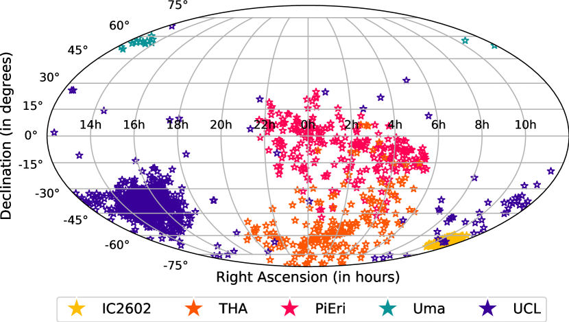
Figure 1: Equatorial locations of stars in selected clusters used in this study

In order to develop and test pterodactyls, we limited our search to only those young clusters in which TESS, along with followup observations with the Spitzer space telescope (Werner et al., 2004), had already found transiting planets during its primary mission: Tucana-Horologium Association (THA), IC 2602, Upper Centaurus Lupus (UCL), Ursa Major (UMa), and Pisces-Eridani (PiEri). DS TUC A b (Newton et al., 2019), HIP 67522 b and c (Rizzuto et al., 2020), TOI 1726 b and c (Mann et al., 2020), and TOI 451 b, c and d (Newton et al., 2021) were discovered using TESS 2-min cadence data and also had Spitzer data. All of these are confirmed planets except for HIP 67522 c. In contrast, the planets in IC 2602 were discovered using 30-min cadence data: TOI 837 b which is a confirmed planet with mass measurements from radial velocity (Bouma et al., 2020), and TIC 460950389 b (Nardiello et al., 2020) which is a Community TESS Object of Interest (CTOI).

In summary, a total of ten planets have been discovered so far in the selected clusters: of them eight were discovered in TESS 2-min cadence data and two in 30-min cadence data. Followup observations have confirmed eight of these while HIP 67522 c and TIC 460950389 b are only candidate exoplanets.

For the selected clusters and associations, we relied on the memberships provided in the BANYAN $\Sigma$ (Gagné et al., 2018) and the Gaia DR2 open cluster member lists (Gaia Collaboration, Babusiaux et al. 2018) which gives us a total of 1940 stars out of which 1591 were observed during the TESS Primary Mission. Based on parameters available in the TIC, these stars span a large range in Gaia G magnitude (1.73-20.45) and stellar mass (0.11-3.2 $M_{\odot}$). Table 1 provides a breakdown of the main properties of the moving groups and clusters that were included in this analysis while Figure 1 shows the relative positions of the clusters and their respective members that were analyzed in this work.

3 Transit Detection Pipeline

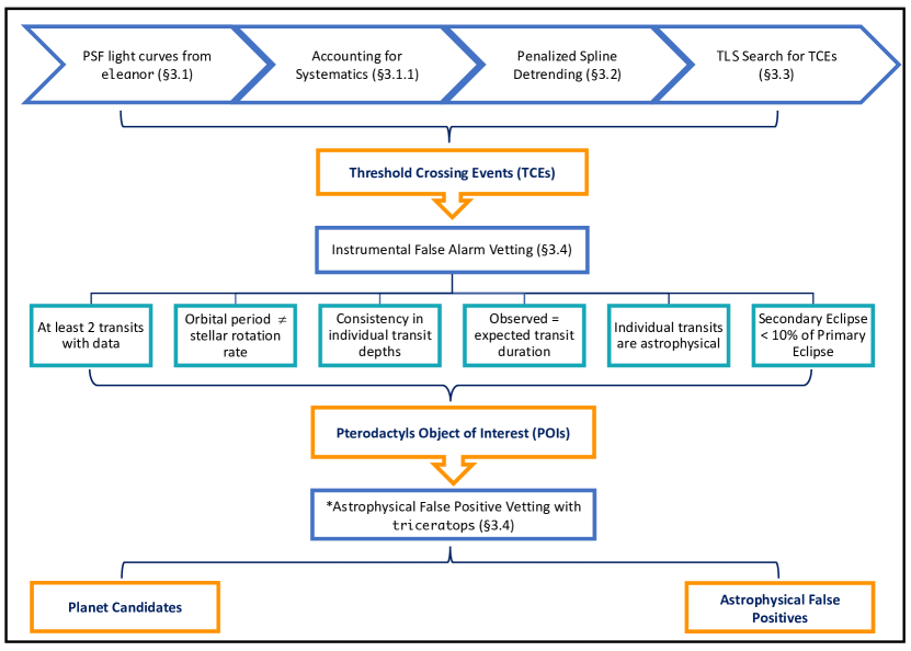
Figure 2: Schematic of pterodactyls. ${}^{\text{*}}$Before passing to triceratops, we conducted a centroid test whenever the Target Pixel File (TPF) was available on MAST.

pterodactyls builds on publicly available and tested tools in order to extract the light curves (Section 3.1), detrend them (Section 3.2), search for transit-like signals (Section 3.3), and vet planet candidates (Section 3.4) in these clusters. We further optimized the efficiency of the detrending, search and vetting components of pterodactyls via injection-recovery tests. For the latter, we injected $\sim$1000 transit signals with planets ranging in size from 0.5-10 $R_{\oplus}$ and with orbital periods between 0.5-10 days into a sample of our light curves using the Python-based batman package (Kreidberg, 2015). We then processed the light curves with pterodactyls and examined the distribution of planets that were recovered. We used this planet distribution as feedback in order to improve pterodactyls. The specifics of the extensive testing using planet injection-recovery tests are summarized in the respective sub-sections while the main steps of the pipeline are summarized in Figure 2.

3.1 Light Curve Extraction

Given that less than 10% of our targets were part of the pre-selected TESS 2-min cadence targets, we use the primary mission’s 30-min cadence photometry extracted from TESS FFIs. Here, we employed eleanor, an open-source tool developed by Feinstein et al. (2019). eleanor carries out background subtraction, and removal of spacecraft systematics such as jitter and pointing drift. eleanor provides four different types of light curves: raw light curves, corrected light curves, light curves with systematics removed using Principle Component Analysis (PCA), and Point Spread Function (PSF) modeled light curves.

In this work, we used PSF-modeled light curves since they better enable the recovery of small signals and minimize the effects of scattered light from the Earth and Moon (Feinstein et al., 2019). eleanor creates these PSF light curves by modeling the shape of the PSF as a multi-variate Gaussian (major axis, minor axis, and a rotation) for each star at each cadence. Then, eleanor integrates that Gaussian function to calculate the flux of the target star at each cadence. The quality flags assigned to the FFI data by the TESS team are implemented during the extraction of the light curves by eleanor (see Table 32 in the TESS Science Data Products Description Document). By default, we only keep the data with the bit value 0 i.e., the highest quality data. Once we download the light curves for each sector for a particular target, we ‘stitch’ them together and run the search on all available Primary Mission data for the target.

3.1.1 Accounting for Systematics

Any instrumental systematics that affect the shape of the PSF, such as the temperature of the instrument, are well-captured by the PSF model and the flux is conserved across it. However, there were several instrumental effects in these light curves that were not captured during the PSF modeling and remain in the light curve such as mid-sector flux drops caused by data downlink, and offsets in the light curves caused by errors in the uploaded Guidestar tables (see TESS’ Data Release Notes for a more detailed description of these issues). Since these instrumental effects would generate spikes in the light curve that affect pterodactyls’ ability to detrend and search for planets, we further optimized these light curves by masking the mid-sector flux drops and re-scaling any offsets. In some cases, eleanor could not properly fit the PSF flux of the target star possibly due to the target being faint, nearby bright stars, etc. We removed 148 such light curves from our sample.

We also masked a number of cadences in sectors 3, 10, 11, and 12 (see Figure  3) because we noticed that they triggered an anomalous number of transit-like detections in the search, indicating an issue with the light curves in those regions. We used a test similar to the “Skye” metric used by Thompson et al. (2018) that was also adopted for K2 data by Zink et al. (2020). The test measures the number of transit-like signals at each cadence and if the number of signals is $>$3$\sigma$, we masked those cadences before re-running the search.

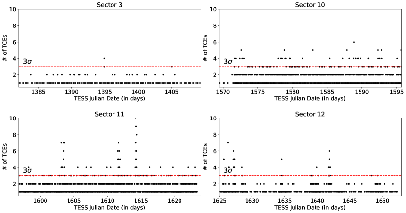
Figure 3: Skye Excess Metric for Sectors 3, 10, 11 and 12 respectively. Red dashed line depicts the 3$\sigma$ threshold.

3.2 Light Curve Detrending

In order to detrend the light curves of these young stars, we explored several options presented in Wōtan, an open-source Python package on GitHub developed by Hippke et al. (2019). In their study, Hippke et al. (2019) used injection recovery tests and found that, in the presence of significant stellar variation, spline-based methods (where adjacent functional pieces join each other at fixed knots) maximized the fraction of injected planets that were recovered. Following up on this result, we tested the following three different spline techniques (see Appendix A for an example): i) a robust spline with iterative sigma clipping, ii) a Huber estimator spline (Huber, 1981) and, iii) a penalized spline with iterative sigma clipping (Eilers & Marx, 1996). We also tested the commonly used Savitzky-Golay filter (Savitzky & Golay, 1964) and found that it often over-fits for the transit thereby causing an inaccurate transit depth measurement, as pointed out in Hippke et al. (2019).

We evaluated the detrending based on the low noise or the root mean square (hereafter, RMS) of the light curve, and recovery fraction from the injection-recovery tests. We found that the penalized spline with iterative sigma clipping works best for our sample of young stars as it gives the lowest RMS measured on a 7-hour window and had the highest recovery fraction ($\sim$92%). We found that, in agreement with Nardiello et al. (2020), the brighter stars contribute more flux and have low RMS. We also see a lot of scatter in the faint star region where there is more flux contamination. Furthermore, the ratio of the recovered planetary radii to the injected radii was close to unity, thereby suggesting that we did not over-detrend our light curves.

In carrying out these tests, we also noticed that the edges of light curves are often challenging to detrend due to the lack of data on one side and would often trigger a search. As such, we decided not to consider 0.5 days worth of data on either edge. We also noticed that the penalized spline uses a cut of 2$\sigma$ i.e., it uses sigma clipping in estimating the trend and does not consider any data that is more than 2$\sigma$ away. While this works well for almost the entire sample, it does not do a good job for light curves with high amplitude ($>$2-3%) rotational signals where it clips out peaks which leaves periodic residuals that are picked up by the search. We manually identified 20 such light curves and applied a 3$\sigma$ cut to them in order to achieve a better detrending.

3.2.1 Optimization Based on Stellar Rotation Rates

A penalized spline is essentially a piecewise polynomial fit in which the routine tries all numbers of splines up to a set maximum, and uses a penalty function to evaluate if a better fit outweighs the added degrees of freedom. The penalized spline provides additional flexibility: unlike other spline methods where the exact number of knots must be chosen manually, the penalized spline identifies the best number of knots by comparing it against the smaller residuals from an improved fit starting from a given maximum number. This feature turns out to be useful for our sample as some young stars are rapid rotators ($<$1 day) with periodic signals on timescales similar to the orbital period. Using injection-recovery tests, we found that the highest planet detection efficiency could be achieved by limiting the maximum number of splines based on the stellar rotation rate.

To this effect, we used a Lomb-Scargle periodogram (Lomb 1976; Scargle 1982; implemented in astropy) to first calculate the stellar rotation rate and then implement the following step function to determine the maximum number of splines that should be used in order to best detrend any given light curve:

• if $R_{\text{rot}}$$\leqslant$ 2 days: max splines = 200

• if $R_{\text{rot}}$$>$ 2 days and $\leqslant$ 10 days: max splines = 200/$R_{\text{rot}}$

• if $R_{\text{rot}}$$\geq$ 10 days: max splines = 25

If the periodogram was not able to find a period, it defaults to the length of the segment (half a sector since there is a break in the middle). Since that is $\sim$10 days, only a small number of splines (25) is used which is ideal for a light curve of low variability. However, this is a maximum number of splines which means that the detrending can still pick the right number of splines even if the rotation period is estimated to be shorter than it really is.

At this stage, we visually inspected all of the light curves and found 80 with variablility trends that were difficult to detrend e.g., extremely fast rotators with a rotational rate $<$0.5 days. Since we were not able to properly detrend these light curves, we also would not have been able to find planets in them. As such, we removed these light curves from our sample and are left with $\sim$1359 light curves that we used to search for planets.

3.3 Planet Candidate Search

We searched the detrended light curves for periodic, transit-like signals with transitleastsquares (hereafter, TLS; Hippke & Heller 2019). TLS is optimized for signal detection of small planets by taking into account the effects of limb darkening to better model the ingress and egress shape (Manduca et al., 1977; Mandel & Agol, 2002). TLS searches for these signals by phase-folding the light curve over a range of epochs, transit durations and orbital periods calculated using a function based on the mass and radius of the host star as detailed in Ofir (2014). The period search grid is set by TLS by dividing the length of the light curve by the minimum number of required transits which is set to two.

For the purposes of our work, we defined a Threshhold Crossing Event (TCE) as having a signal-to-noise ratio (SNR) of 7 and a signal detection efficiency (SDE) of 7. Most transit survey studies choose an SDE value between 6 and 10 (see e.g., Dressing & Charbonneau 2015; Livingston et al. 2018; Siverd et al. 2012; Pope et al. 2016; Aigrain et al. 2016; Feliz et al. 2021). While a lower SDE would mean higher completeness, a higher SDE would reduce the number of false positives. Our chosen SNR and SDE cuts reduced the number of false positives, which arose from detrending artifacts caused by the significant ($\sim$20%) number of rapid rotators with periodic signals comparable to stellar rotation rates. Additionally, an SNR and SDE cut of 7 recovers eight out of the ten the previously detected planets (see Section 5.1).

3.4 Candidate Vetting

Transiting surveys (like Kepler, K2 and TESS) that target a large number of stars face a major challenge while distinguishing false alarms (transit-like events caused by instrumental artifacts) and astrophysical false positives (transit-like events that are astrophysical in origin but are not caused by planets). The process of sorting out false alarms and false positives from real transit signals is known as vetting. In order to filter out any instrumental false alarms that could be due to detrending artifacts, we used criteria inspired by RoboVetter (Kepler; Thompson et al. 2018) and EDI-Vetter (K2; Zink 2019; Zink et al. 2020) to create four checks in order to address the issues unique to our sample. Only the TCEs that pass the following tests are considered objects of interest:

• At least two transits with data: We required two transit signals with in-transit data points in a given light curve which allowed us to find planets with orbital periods of up to 13.5 days around most of the stars (assuming each star only had single sector data). If we required at least three unique transits like Kepler did, we would be limited to transit signals with orbital periods less than 9 days.

• Orbital period dissimilar to stellar rotation rate: While analysing the results of the search, we often found residuals at orbital periods similar ($\sim$20%) to the stellar rotation rate (and some of these at half the rotation rates), despite detrending. To combat this, we flag any such TCEs.

• Consistency in individual transit depths: We found that, quite often, false alarms have transit depths with larger variance than real planets. Similar to Kepler’s Robovetter Single Event Statistic (SES), we flagged signals with large variations in transit depth as likely false positives. We weed out these signals based on the ratio of the standard deviations of the individual transit depths to the average transit depth, which we set to be greater than 1.5 for a false positive. This cutoff was determined by preserving known planets while keeping the number of false positives low.

• Observed transit duration should be consistent with expected transit duration: On visual inspection, we found that some TCEs had transit durations that were inconsistent with those of planetary transits. For example, stellar variability can lead to dips with a duration longer than a transit, and single occurrence outliers can appear to have a shorter transit duration. In such cases, it is beneficial to compare the observed transit duration to the expected transit duration that is determined using the planetary parameters calculated by TLS. If the observed transit duration is within 75% of the expected transit duration, the TCE passes this test. This cut was also set to preserve known planets and reduce the number of false positives.

In addition, we also used two checks from EDI-Vetter Unplugged (Zink et al., 2020) that were initially designed to vet transits in K2 data but has now been adapted to vet TESS light curves (for e.g., see Feliz et al. 2021).

• Individual Transit Test: Derived from the Marshall test designed by Mullally et al. (2016) for Kepler, this test used transit models and those of common non-transiting false positives and fit these to the individual transits. It then used the Bayesian Information Criterion (BIC) to gauge the goodness of these fits, thereby flagging the non-transiting signals that are often assumed to belong to transiting planets.

• Secondary Eclipse Test: This test looked for transit events between the 40-60% phase range of the folded light curve, allowing for some mild eccentricity variations. If a meaningful secondary eclipse was identified i.e., the secondary eclipse has a transit depth $>$10% of the primary transit, this flag was triggered and the transit was labeled a false positive. Secondary eclipses with less than 10% depth can be associated with reflected light from hot Jupiters.

Once we removed the clear false alarms and only have transit-like signals, we were left with 21 pterodactyls Objects of Interest (hereafter POIs; see Tables 2 and 3) on which we conducted a centroid test (Hedges, 2021) in order to determine whether the transiting signal was indeed coming from the target star (see Appendix C). This test compares the distributions of centroids for the data inside and outside the transit. An offset would indicate that the transiting signal was coming from a contaminating source such as a nearby or background star. We chose a probability p of 5% for the Student t-test below which the centroids positions inside and outside transits are not considered to come from the same parent distribution.

All POIs were then passed on to triceratops (Giacalone et al., 2021) $-$ a vetting tool designed to distinguish bona fide planets from astrophysical false positives in TESS data. triceratops calculated the marginal likelihood of each transit-producing scenario using observational constraints such as the transit depth and transit duration from TLS for each potential host, positions and magnitude of nearby stars from Gaia dr2 (Gaia Collaboration et al., 2018), priors on planet occurrence and stellar multiplicity rates, and models of planetary transits and eclipsing binaries. These scenarios include transiting planets and eclipsing binaries originating from the target star, known nearby stars, and unknown unresolved stars located near the target on the sky. Lastly, triceratops calculates the Bayes factor between all scenarios involving a transiting planet around the target star and all astrophysical false positive scenarios. Using this Bayes factor, triceratops can place a statistically robust constraint on the reliability of any given planet candidate detected by TESS. Here, we made a transiting planet probability cut of 50% in order to preserve known planets.

4 Fitting for Planet Properties

Once the POIs have passed all of the vetting tests described in Section 3.4, we fit the phase-folded light curve in order to derive a more accurate planet radius. Since TLS only provided an initial fit to the phase-folded light curve and did not provide uncertainties on the planet radius, we used TLS’ outputs as priors for a more rigorous optimization in order to derive uncertainties using EXOTIC (Zellem et al., 2020). Here, the transit parameters are optimized using the multi-modal nested sampling algorithm called UltraNest (Buchner, 2021) which is a Bayesian inference tool that uses the Monte Carlo strategy of nested sampling to calculate the Bayesian evidence allowing simultaneous parameter estimation and model selection. A nested sampling algorithm is efficient at probing parameter spaces which could potentially contain multiple modes and pronounced degeneracies in high dimensions; a regime in which the convergence of traditional Markov Chain Monte Carlo (MCMC) techniques becomes incredibly slow (Skilling 2004; Feroz & Hobson 2008). This approach has been validated on Kepler light curves, TESS data and ground-based measurements (Pearson et al., 2018, 2019; Pearson, 2019).

5 Results

We processed $\sim$1359 young stellar light curves extracted from TESS FFIs i.e., 30-min cadence data through pterodactyls (see Appendix D for the TIC IDs processed in this work). As an illustration, Figure 4 shows the different steps that were used in the recovery of the planet TOI 451 d. We detected 21 POIs that were then passed to triceratops where their phase-folded light curves were vetted to separate transiting planet signals from astrophysical false positives.

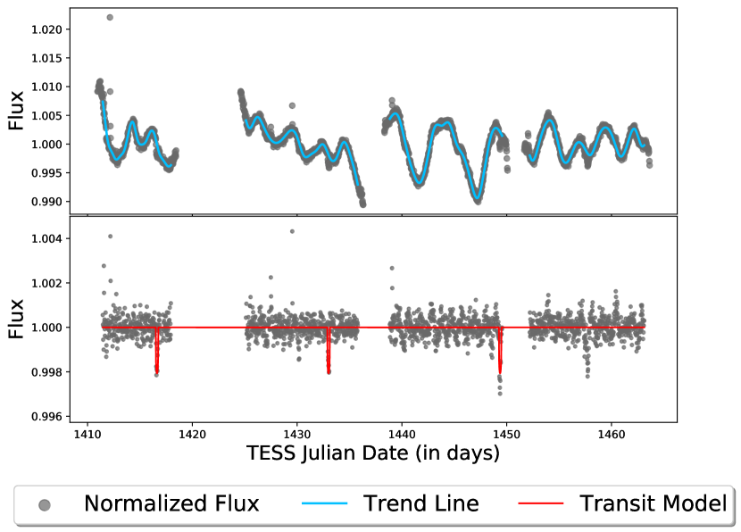
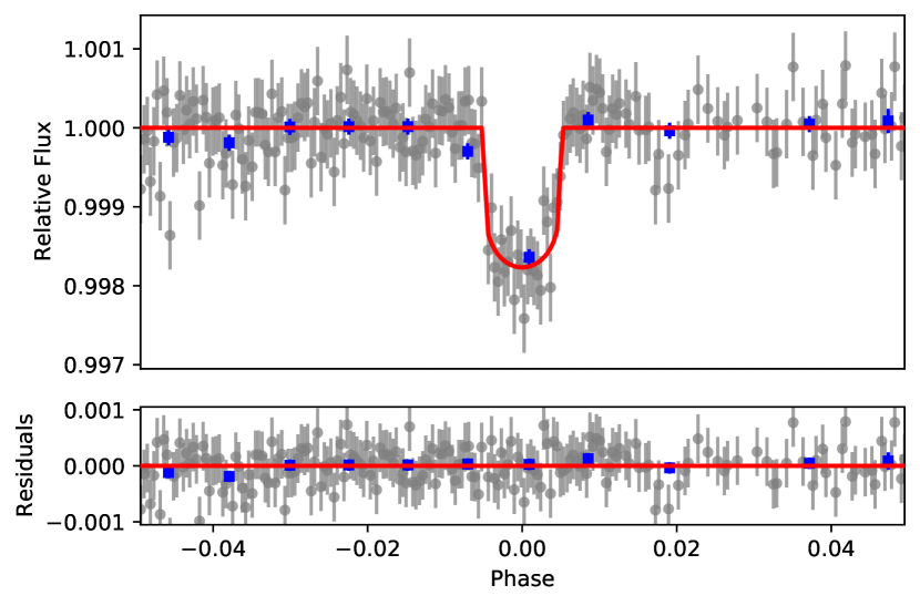
Figure 4: Left: Recovery of TOI 451 d. Upper panel: PSF flux (in dark gray) and penalized spline trend (in blue). Lower panel: Detrended light curve (PSF flux divided by the trend). The multi-transit signature (in red) can be clearly seen. Right: Upper panel shows Phase-folded light curve of TOI 451 d (gray data points) along with the best fit model using EXOTIC (in red). Lower panel shows the residuals in parts per million.

5.1 Recovery of Known Exoplanets

Planet	Ref.	Cluster	Radius (pub; $R_{\oplus}$)	Period (pub; days)	Radius (rec; $R_{\oplus}$)	Period (rec; days)	TP prob %
DS Tuc A b∗	a	THA	5.70$\pm$0.17	8.138268$\pm$0.000011	$5.349^{+0.464}_{-0.458}$	8.215$\pm$0.066	54.93
TIC 460950389 b	b	IC 2602	3.8$\pm$0.2	2.8622$\pm$0.0004	$3.554^{+0.320}_{-0.304}$	2.861$\pm$0.005	99.69
TOI 837 b	b,c	IC 2602	$6.9^{+0.6}_{-0.4}$; $8.90^{+0.74}_{-0.71}$	8.3252$\pm$0.0006	$7.224^{+0.410}_{-0.387}$	8.325$\pm$0.016	97.45
HIP 67522 b∗	d	UCL	$9.72^{+0.48}_{-0.47}$	6.95993$\pm$0.00034	$13.400^{+1.354}_{-1.328}$	6.893$\pm$0.019	86.06
HIP 67522 c∗	d	UCL	$8.01^{+0.75}_{-0.71}$	$54^{+70}_{-24}$	xx	xx	xx
TOI 1726 b∗	e	UMa	2.15$\pm$0.10	$7.10793^{+0.00046}_{-0.00034}$	$2.134^{+0.214}_{-0.213}$	7.116$\pm$0.043	75.32
TOI 1726 c∗	e	UMa	2.67$\pm$0.12	20.5455$\pm$0.0011	$2.225^{+0.264}_{-0.267}$	20.5234$\pm$0.1022	75.72
TOI 451 b∗	f	PiEri	$1.94^{+0.15}_{-0.34}$	$1.858701^{+0.000027}_{-0.000033}$	xx	xx	xx
TOI 451 c∗	f	PiEri	3.07$\pm$0.14	$9.192523^{+0.000064}_{-0.000084}$	$2.604^{+0.308}_{-0.294}$	9.195$\pm$0.036	71.11
TOI 451 d∗	f	PiEri	4.03$\pm$0.15	$16.364981^{+0.000047}_{-0.000049}$	$3.678^{+0.306}_{-0.294}$	16.368$\pm$0.070	70.63

Table 2: Published and Recovered Properties of planets detected in young clusters. References: a) Newton et al. (2019); b) Nardiello et al. (2020); c) Bouma et al. (2020); d) Rizzuto et al. (2020); e) Mann et al. (2020); f) Newton et al. (2021) ^∗Planet originally detected in 2-min cadence data.

In the five clusters that were searched in this work, there are eight confirmed planets and two planet candidates. More specifically, three were single planet systems (DS Tuc A b, TIC 460950389 b, and TOI 837 b; the latter two discovered in 30min-cadence data) and seven were part of three multi-planet systems (HIP 67522 b and c, TOI 1726 b and c, and TOI 451 b, c and d), all discovered in 2-min cadence data (see Section 2). As pterodactyls, which is automated, is built to search for just one planet per star, the discovery of additional planets in a system is carried out after finding a first planet and masking it out.

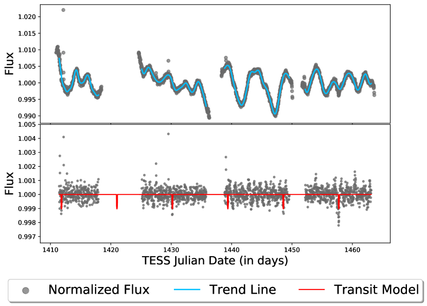
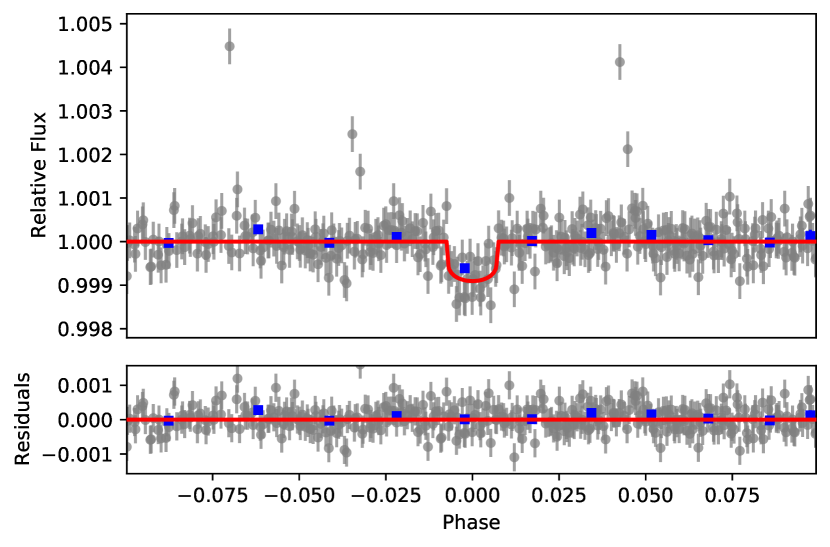
Figure 16: Left: Recovery of TOI 451 c. Upper panel: PSF flux (in dark gray) and penalized spline trend (in blue). Lower panel: Detrended light curve (PSF flux divided by the trend). The multi-transit signature (in red) can be clearly seen. Right: Upper panel shows Phase-folded light curve of TOI 451 c (gray data points) along with the best fit model using EXOTIC (in red). Lower panel shows the residuals in parts per million.

Among the 21 POIs detected by pterodactyls in the first automated run, we find six of the confirmed exoplanets that were previously detected by various teams using TESS (summarized in Table 2; for light curves, see Appendix B). pterodactyls was able to recover the values for the orbital periods and radii for three of these planets that were consistent (within uncertainties) with the literature. This includes two single planets (TIC 460950389 b, and TOI 837 b) that were initially discovered in 30-min cadence data, and one multi-planet system (TOI 451 b, c and d) that was initially discovered in 2-min cadence data. We first recovered TOI 451 d (4.1 $R_{\oplus}$) at an orbital period of 16.36 days. After masking this transit, we were also able to recover TOI 451 c (3.1 $R_{\oplus}$) at 9.19 days (see Figures 4 and 16). However, pterodactyls was not able to recover TOI 451 b (1.9 $R_{\oplus}$) since it has a low SNR ($\sim$5). We find that all of the confirmed planet and planet candidates that pterodactyls recovers pass the centroid test.

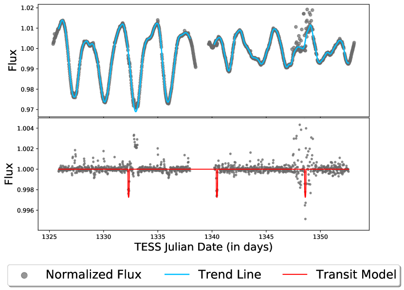
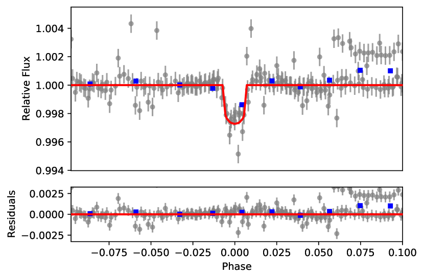
Figure 11: Left: Progression of the DS Tuc A light curve through pterodactyls. Upper panel: PSF flux (in dark gray) and penalized spline trend (in blue). Lower panel: Detrended light curve (PSF flux divided by the trend). The multi-transit signature (in red) can be clearly seen. Right: Upper panel shows Phase-folded light curve of DS Tuc A b (gray data points) along with the best fit model using EXOTIC (in red). Lower panel shows the residuals in parts per million.

Two out of the other three recovered transiting systems (out of a total of six as stated above) suffered from sparse cadence (few in-transit data points): DS Tuc A b and HIP 67522 b. For these, pterodactyls was able to accurately recover the orbital periods but not the same radii as in the literature. In the case of DS Tuc A b, at first we considerably underestimated the planet’s radius value. On further inspection, we noticed that this was caused by very few in-transit data points that was due to the removal of “bad” data that was flagged using the TESS team’s quality flags. In this specific case, we found that inclusion of certain quality flags lead to a better estimation of the planetary radius i.e 5.35 $R_{\oplus}$(see Figure 11) which is within errors of the value of 5.70 $R_{\oplus}$that was measured using TESS’ 2-min cadence and Spitzer data (see Table 2). In the case of HIP 67522 b, the overestimation of the planet radius was severe: we recovered a radius of 13.4 $R_{\oplus}$while the planet’s observed radius is 9.72 $R_{\oplus}$. This could be due to several factors. First, as can be seen in Figure 5, the middle transit was not recovered (but predicted by TLS) due to the default edge cutoff for all stars being 0.5 days. However, the severe overestimation of the radius could also be due to the planet being discovered in the more abundant 2-min cadence data. We tested this by processing the publicly available 2-min cadence light curve through pterodactyls (see Figure 6) and found that with the increased number of in-transit data points (along with higher RMS compared to 30-min cadence data), we were able to recover a planet radius of 9.8 $R_{\oplus}$which is close to the literature value of 9.72 $R_{\oplus}$. We were not able to recover HIP 67522 c due to it being a single transit event and hence, beyond the scope of pterodactyls since it requires a minimum of two transits.

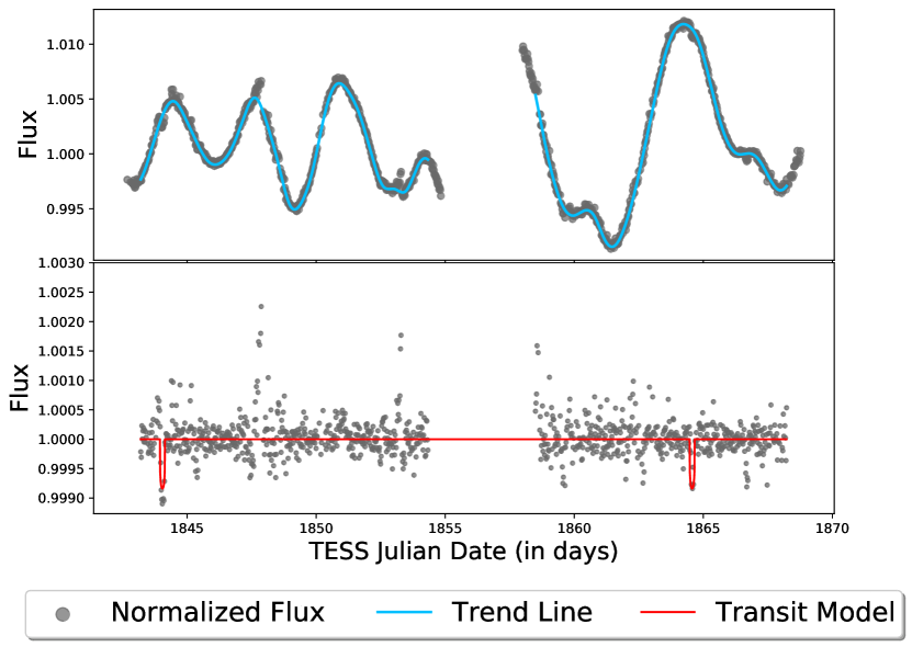
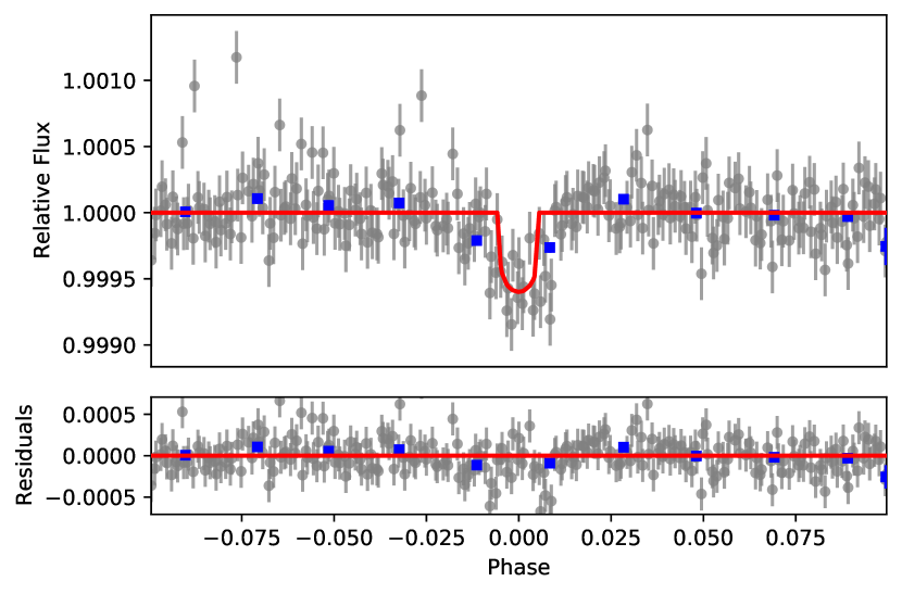
Figure 14: Left: Recovery of TOI 1726 c. Upper panel: PSF flux (in dark gray) and penalized spline trend (in blue). Lower panel: Detrended light curve (PSF flux divided by the trend). The multi-transit signature (in red) can be clearly seen. Right: Upper panel shows Phase-folded light curve of TOI 1726 c (gray data points) along with the best fit model using EXOTIC (in red). Lower panel shows the residuals in parts per million.

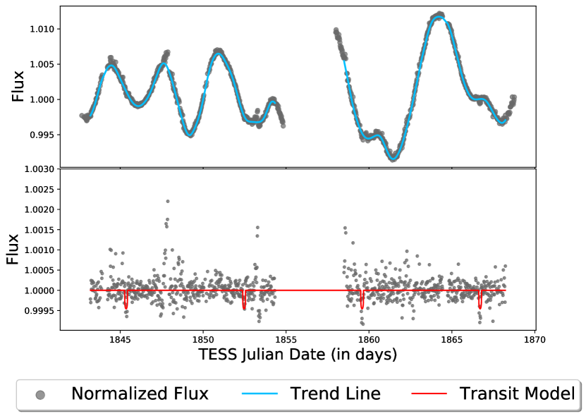
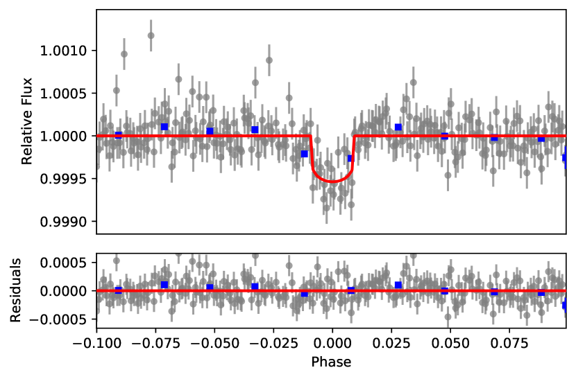
Figure 15: Left: Recovery of TOI 1726 b. Upper panel: PSF flux (in dark gray) and penalized spline trend (in blue). Lower panel: Detrended light curve (PSF flux divided by the trend). The multi-transit signature (in red) can be clearly seen. Right: Upper panel shows Phase-folded light curve of TOI 1726 b (gray data points) along with the best fit model using EXOTIC (in red). Lower panel shows the residuals in parts per million.

Finally, for the TOI 1726 system in UMa, we recovered a transit signal from a 2.48$R_{\oplus}$ planet with an orbital period of 11.32 days. However, the TOI-1726 system has two small planets (b and c) of radii 2.15 $R_{\oplus}$and 2.67 $R_{\oplus}$, with orbital periods of 7.11 and 20.55 days respectively (Mann et al., 2020). Given that the planet sizes (and hence, transit depths) are similar, the signals were initially detected by pterodactyls as coming from one planet. Upon further inspection, we realized that TLS set the maximum orbital period in the grid based on the minimum number of transits. So, for single sector data ($\sim$27 days) with the minimum number of transits set to 2, the maximum orbital period would be $\sim$13.5 days which is shorter than the orbital period of TOI 1726 c. With this in mind, for this case alone, we set the minimum number of transits to one and were able to recover TOI 1726 c (see Figure 14). We then masked this transit and re-processed it through pterodactyls and recovered TOI 1726 b as well (see Figure 15).

After implementing the aforementioned fixes, we find that all of the recovered orbital periods are the same as those reported in the discovery papers while for the radii, four are the same within 1$\sigma$ and three within 2$\sigma$ (Figure 7). The recovery of these planets demonstrates the usefulness of pterodactyls in discovering young planets in 30-min cadence data.

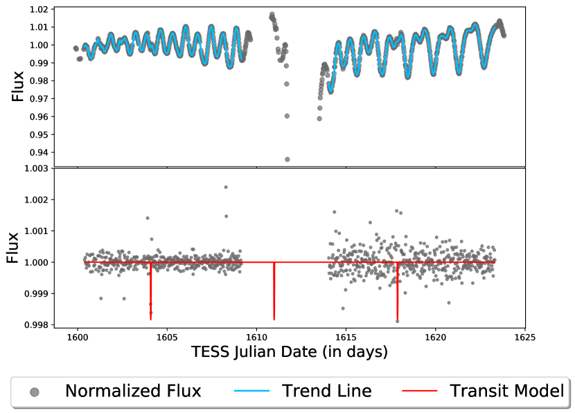
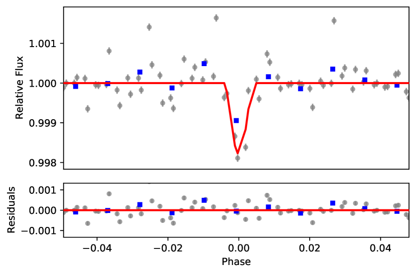
Figure 5: Left: Recovery of HIP 67522 b. Upper panel: PSF flux (in dark gray) and penalized spline trend (in blue). Lower panel: Detrended light curve (PSF flux divided by the trend). The multi-transit signature (in red) can be clearly seen. Right: Upper panel shows Phase-folded light curve of HIP 67522 b (gray data points) along with the best fit model using EXOTIC (in red). Lower panel shows the residuals in parts per million.

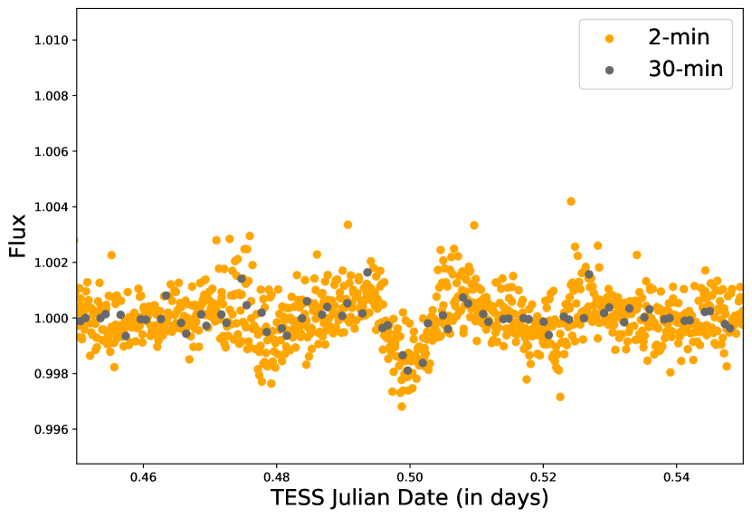
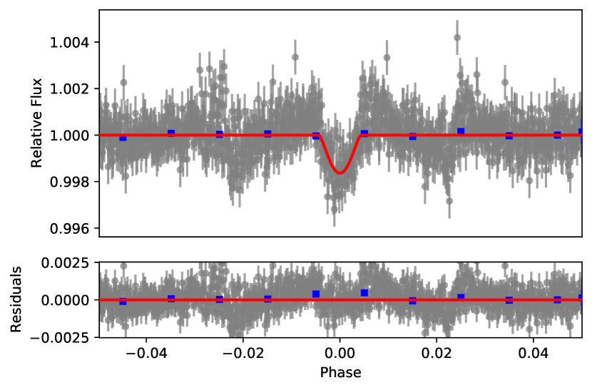
Figure 6: Left: Comparison of phase-folded light curve of HIP 67522 b using 2-min cadence data (orange) and 30-min cadence data (black). Right: Upper panel shows Phase-folded light curve of HIP 67522 b using 2-min cadence (dark gray points) along with the best fit model using EXOTIC (in red). Lower panel shows the residuals in parts per million.

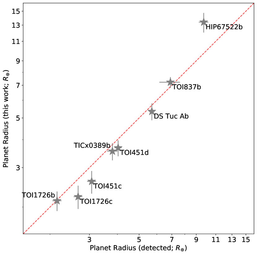
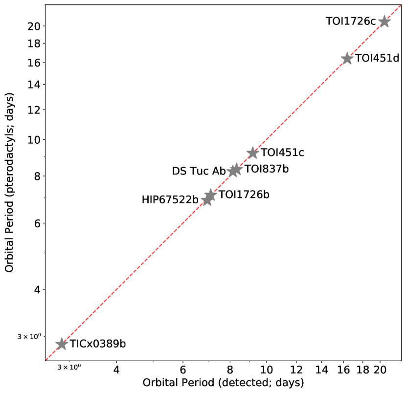
Figure 7: Left: Comparison of planetary radii recovered using pterodactyls (fitted with EXOTIC) vs. known planet radii for the eight recovered known planets. As can be seen, despite being recovered from 30-min cadence data, the radii are often consistent with those published. In two cases, TOI 1726 c and TOI 451 c, we slightly underestimate the planet’s radius. We also overestimate the radius of the planet for HIP 6752 b. Right: Comparison of orbital periods recovered using pterodactyls vs. known orbital periods for the eight recovered planets to depict consistency between the results of our work and those from the discovery papers. Note: Orbital period errors are extremely small and hence cannot be seen in the plot.

5.2 Astrophysical False Positives Vetting

Apart from the six confirmed planets, pterodactyls also detected 15 other POIs (see Table 3), including two eclipsing binary signals around two stars in UCL i.e., TIC 129116176 and TIC 148158540. We weren’t able to conduct centroid tests on all of these targets since the Target Pixel File on the MAST server (which is used for the centroid test) were only available for three of the candidates (all of the ones in UCL) in Table 3 but not for the 12 other candidates (IC2602). As such, we conducted the centroid test whenever the data was available. For the targets, where we could not conduct the centroid test, we visually inspected the eleanor pixel by pixel light curves. While determining the probability of a transiting signal being due an astrophysical false positive or a transiting planet, triceratops (by default) takes into account planet occurrence rates priors that are based on the Gyr-old exoplanet population (e.g., Howard et al. 2012; Dong & Zhu 2013; Petigura et al. 2013; Dressing & Charbonneau 2015; Mulders et al. 2015, 2018). However, if the planet population around young stars is different from that around Gyr-old stars, for example because young planets are larger in size, the probability that triceratops would calculate is likely to be biased. In order to test the effect of priors on the probabilities of the different scenarios investigated by triceratops, we also calculated the astrophysical false positive probability using non-informative (flat) priors that were recently implemented in triceratops.

Out of our remaining 15 POIs, we found that 11 were not affected by the choice of priors and had the same probability of being an astrophysical false positive in both cases. In two out of the remaining four, we detected a transiting signal in each each of them (TIC 466579089 and TIC 466035035; see Table 3) that had passed all our vetting tests. Using Gyr-old priors, triceratops calculated the most likely scenario to be a nearby eclipsing binary (NEB). However, when using flat priors, the most likely probability was calculated to be a transiting planet. Given that IC 2602 is an extremely crowded cluster ($\sim$5 stars per TESS pixel), we used eleanor’s pixel level light curves to investigate whether these transits were indeed around our target stars. In doing this, we found that the signal was coming from giant stars (TIC 466579123 and TIC 466035000, respectively) a couple of pixels away and actually contributed more flux to the pixel than our target star. With this information in hand, we ran pterodactyls on those stars and were able to detect the same signal in the light curve but, this time, triceratops found that the most likely scenario was that the signal was due to an eclipsing binary around TIC 466579123 and TIC 466035000.

When the false positive probability was calculated using flat priors, the remaining two POIs that were initially calculated to be nearby eclipsing binaries with Gyr-old priors, showed a $>$25% chance that the signal was either a nearby eclipsing binary or a nearby transiting planet. These POIs have large transits depths that could either be attributed to small stars, brown dwarfs or giant planets since the two populations have comparable radius distributions (Chen & Kipping, 2017). This, along with the fact that identifying shallow secondary transits can be arduous, makes it harder for statistical validation tools such as triceratops to properly distinguish between these scenarios (Shporer et al., 2017). In cases such as these, masses obtained via radial velocity follow-up are necessary to differentiate between these scenarios. This illustrates the need to properly take into account flux contamination in young clusters while vetting planet candidates.

TIC ID	Cluster	Period (d)	Most likely (Gyr-old priors)	Most likely (Flat priors)	Potential Host Star(s)
390758843	IC 2602	0.890	25% NEB	25% NEB	TIC 390758947
376731139	IC 2602	12.769	50% NEBx2P	49% NEBx2P	TIC 376731097
911870867	IC 2602	20.018	42% NEB	40% NTP; 27% NEB	TIC 390843430
911870847	IC 2602	20.018	50% NEB	37%NEB; 30% NTP	TIC 390843430
315312718	IC 2602	2.203	28% NEB	30% NEB	TIC 315312721; TIC 315312651
466035035	IC 2602	1.522	99% EB	92% TPx	TIC 466035000
466579089	IC 2602	15.910	91% NEB	44% NEB; 44% TPx	TIC 466579123
913701079	IC 2602	2.900	88% NEBx2P	84% NEBx2P	TIC 465306570
465306494	IC 2602	2.899	86% NEBx2P	85% NEBx2P	TIC 465306570
378611172	IC 2602	7.542	89% NEBx2P	87% NEBx2P	TIC 378611218
466422383	IC 2602	33.247	99% NEBx2P	99% NEBx2P	TIC 466422466
390757974	IC 2602	1.705	54% NEB	54% NEB	TIC 390758017
177631209	UCL	2.144	32% EB	21% PEB; 21% NEB	TIC 177631209; TIC 1167076020
129116176	UCL	4.032	74% EBx2P	91% EBx2P	-
148158540	UCL	3.700	65% EBx2P	64% EBx2P	-

Table 3: List of POIs/Potential Binaries detected by pterodactyls and vetted using triceratops in both Gyr-old and flat prior mode. Key: TP = Transiting Planet around Target Star; EB = Eclipsing Binary around Target Star; EBx2P = Eclipsing Binary around Target Star with twice the orbital period compared to what was detected by TLS; NTP = Nearby Transiting Planet; NEB = Nearby Eclipsing Binary; NEBx2P = Nearby Eclipsing Binary with twice the orbital period compared to what was detected by TLS; PEB: Eclipsing Binary around Primary Star with Unresolved Bound Companion. ^xSee discussion in Section 5.2 Note: The signals found in TIC 911870867 & TIC 911870847 as well as TIC 913701079 & TIC 465306494 have similar orbital periods with the same potential host star suggesting that they might be blended or part of the same multiple system.

6 Planet Occurrence Rates in investigated clusters

6.1 Detection Efficiency

An advantage of having an automated planet detection pipeline is that it enables the measurement of the survey detection efficiency which is necessary to compute intrinsic occurrence rates. The detection efficiency of our survey was calculated using injection-recovery tests on a 3$\times$4 grid in $\frac{R_{\text{p}}}{R_{\star}}$  from 0.01 to 0.3 and in orbital period from 0.5 to 27 days , equally spaced in both $\frac{R_{\text{p}}}{R_{\star}}$and orbital period. The injections are carried out in the $\frac{R_{\text{p}}}{R_{\star}}$ space because most stars in our clusters currently lack stellar properties. We injected a transit signal in each bin in each light curve in our sample while taking into account the flux contribution of each star as calculated by triceratops. We then passed these injections through pterodactyls and calculated the fraction that were recovered as planets to produce a detection efficiency map per cluster as well as an average map for the entire sample. The average detection efficiency map is presented in Figure 8 and shows that the overall detection efficiency does not exceed 50% for any bin below 0.1 $\frac{R_{\text{p}}}{R_{\star}}$(i.e., a Jupiter-sized planet assuming it orbits a Sun-like star). Interestingly, all the previously known recovered planets (denoted using blue stars in Figure 8) are in bins with fairly low values ($<$20%). This might be due to the intrinsic occurrence of smaller vs. larger planets being higher (Mulders et al., 2015; Petigura et al., 2018; Mulders et al., 2018).

We also investigated how the detection efficiencies of each cluster contributed to the overall detection efficiency. Figure 9 illustrates that the detection efficiency of a cluster can be quite different from the average. For example, Pisces-Eridani (top panel) has a significantly larger detection efficiency. IC 2602 (middle panel), on the other hand, has an extremely low detection efficiency. These differences might be due to age (IC 2602 is younger, hence its stars might be more variable) and/or to flux contamination due to stellar crowding, which is significantly more pronounced in IC 2602.

We further investigated the effects of flux contamination on IC 2602’s detection efficiency by re-running the injection recovery tests without accounting for flux contamination. In other words, signals are injected into the light curve assuming that all of the flux comes from the target star and hence, there is no transit depth dilution. The detection efficiency map is given in the bottom panel of Figure 9 and it is similar to that of Pisces Eridani within 10 days and above 0.06$\frac{R_{\text{p}}}{R_{\star}}$. This test demonstrates that flux contamination significantly reduces the detectability of all planets but stellar variability in the youngest associations still plays a role for the smaller planets.

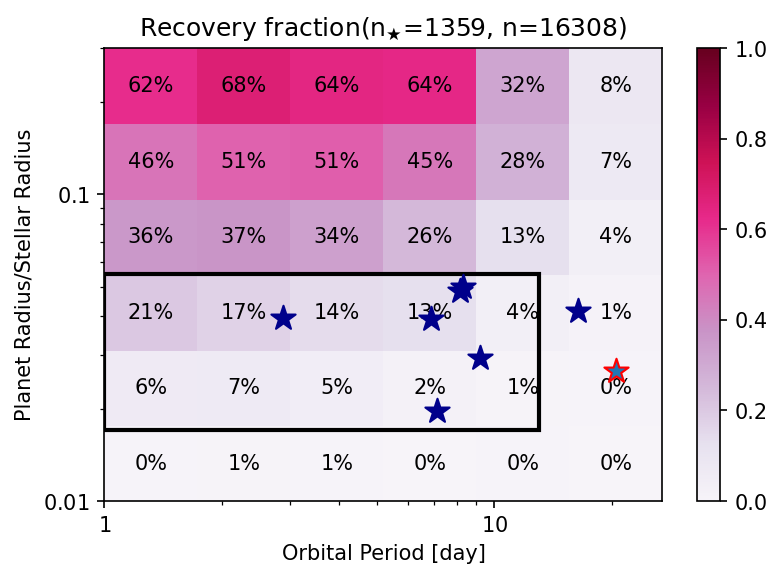
Figure 8: Overall detection efficiency of pterodactyls while taking into account flux contamination. The confirmed planets are depicted using blue stars, except for TOI 1726 b whose recovery required changing pterodactyls. Darker bins represent regions of higher detection efficiency. ${n_{\star}}$ is the total number of stars in our sample while n is the total number of injections done. Black box denotes the bin over which the intrinsic occurrence rates were calculated i.e., sub-Neptunes and Neptunes (0.017-0.055 $\frac{R_{\text{p}}}{R_{\star}}$ or 1.8-6 $R_{\oplus}$, assuming a solar radius) within 12.5 days (about half a TESS sector).

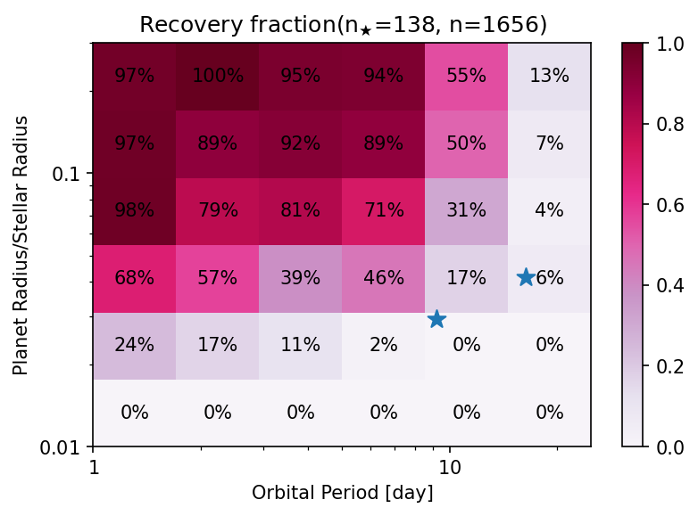
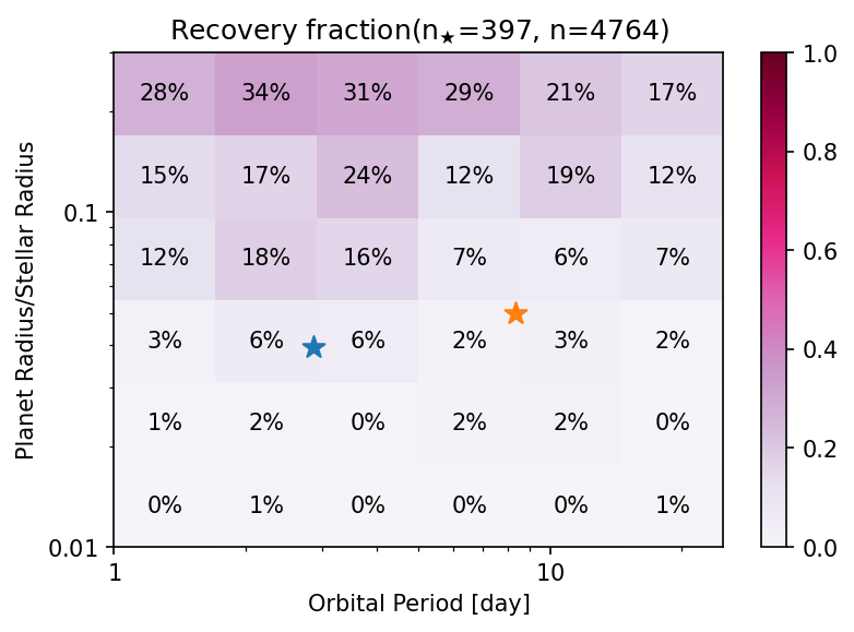
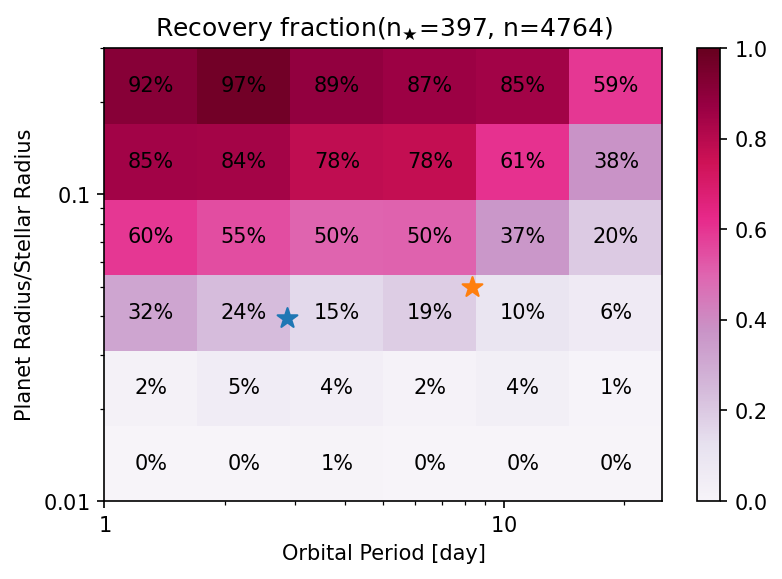
Figure 9: A comparison of extreme detection efficiencies to highlight the effect of flux contamination: Top: Detection efficiency of Pisces-Eridani, a moving group with members that are spread out so flux contamination is minimal. Middle: Detection efficiency of IC 2602, a crowded cluster, while taking into account flux contamination while injecting planets. Bottom: Detection efficiency of IC 2602 while assuming no flux contamination while injecting planets.

6.2 Preliminary Calculation of Occurrence Rates

The intrinsic occurrence rate of planets ($\eta$) can be calculated from the fraction of stars with detected planets in a survey and the survey completeness. Here, we used the inverse detection efficiency method as follows:

$$\eta=\frac{{n_{\text{p}}}}{n_{\star}}*\frac{1}{comp_{\text{bin}}}$$ (1)

where $comp_{\text{bin}}$ is the survey completeness evaluated in the defined bin, $n_{p}$ is the number of detected planets in the bin and $n_{\star}$ is the number of surveyed stars. The survey completeness is computed by combining the detection efficiency and the geometric transit probability, which is given by

$$f_{\text{geo}}=\frac{R_{\star}}{a}$$ (2)

Here, $R_{\star}$ is the stellar radius, and $a$ is the average semi-major axis which is calculated using Kepler’s third law. The uncertainty on the occurrence rate was calculated from the square root of the number of detected planets in the bin, assuming Poissonian statistics.

In our analysis, we only considered sub-Neptunes and Neptunes (0.017-0.055 $\frac{R_{\text{p}}}{R_{\star}}$ or 1.8-6 $R_{\oplus}$, assuming a solar radius) within 12.5 days (about half a TESS sector) because we wanted to understand the primordial population of sub-Neptunes and Neptunes before being stripped off of their atmospheres. With an average detection efficiency of 9% and a $f_{\text{geo}}$ of 0.1 (at a geometric mean orbital period of 3.5 days and assuming a Solar-type star), we compute an occurrence rate of 49$\pm$20% for our sample of young clusters.

We then use epos (Mulders et al., 2018) to calculate the Kepler Gyr-old FGK (Sun-like) occurrence in the same bin. epos is a well documented and tested Python code developed by our team, it is available on GitHub, and has already been used in several publications to compute occurrence rates as well as to compare planet formation models to the Kepler exoplanetary systems (e.g., Kopparapu et al., 2018; Pascucci et al., 2018; Fernandes et al., 2019; Mulders et al., 2019; Pascucci et al., 2019; Mulders et al., 2020). Here, we computed an occurrence rate value of 6.8$\pm$0.3%, which is much lower than our computed value for young clusters. This could be attributed to several reasons, the major one being that our sample is heavily biased towards clusters with known planets. For example, if we increased the sample of young stars to search by a factor of six, which is about all nearby young stars within $\sim$200 pc and assumed the same detection efficiency with no new planets, the occurrence would drop to $\sim$8% which is the same as the Kepler value. Furthermore, since most of the stars in the sample do not have stellar radii, masses or effective temperatures, it is very likely that we are considering non-FGK stars, most likely lower mass stars (Henry et al., 2006; Winters et al., 2014), while calculating the occurrence rate which would make the comparison to Kepler inaccurate, where the sample is mostly Sun-like stars. Therefore, in order to better estimate the occurrence rates of planets in young clusters, we will need to expand our search to all nearby clusters, measure the stellar parameters for those stars, and only compute the occurrence for FGK stars in our sample. However, if we continue to see this increased occurrence after we expand our sample to include all nearby clusters and moving groups, it could imply that there is an excess of larger planets at young ages possibly because their atmospheres have not yet been stripped due to photoevaporation and/or core-powered mass loss.

7 Summary and Future Work

In this paper, we present pterodactyls $-$ a Python-based pipeline that is built using publicly available codes, and is specifically designed to extract, detrend, search for, and vet transiting exoplanets in young clusters using TESS’ Primary Mission 30-min cadence FFIs. Here, we only consider 5 specific young clusters and moving groups: Tucana-Horologium Association, IC 2602, Upper Centaurus Lupus, Ursa Major, and Pisces Eridani. These clusters were chosen solely due to the presence of eight confirmed planets and two candidates which were used to validate pterodactyls. Using pterodactyls,

• We were able to recover eight out of ten known transiting planets/candidates. For the two that we were not able to recover (both initially discovered using 2-min cadence data), one planet was too small to detect (PiEri; TOI 451 b) and the other is a long period, single transit planet (UCL; HIP 67522 c), which is beyond the capabilities of the pipeline.

• We also detected 15 transiting signals, all of which were found to be either eclipsing binaries or nearby eclipsing binaries when their phase-folded light curves were vetted by triceratops.

• While taking into account the stellar flux contribution, we conducted injection-recovery tests in order to measure the detection efficiency of the pterodactyls. We found that the overall detection efficiency does not exceed 50% for any bin below 0.1 $\frac{R_{\text{p}}}{R_{\star}}$(i.e., a Jupiter-sized planet orbiting a Sun-like star) and that all the recovered planets are in bins with fairly low values ($<$20%), hinting that even in young clusters smaller planets are more frequent than giant planets.

• For our biased sample, we computed a planet occurrence rate of 49$\pm$20% which is significantly higher than Kepler’s Gyr-old occurrence rates of 6.8$\pm$0.3% for sub-Neptunes and Neptunes (0.017-0.055 $\frac{R_{\text{p}}}{R_{\star}}$ or 1.8-6 $R_{\oplus}$, assuming a Solar radius) within 12.5 days (about half a TESS sector).

Since most of these planets were initially detected in 2-min cadence data, our work shows that 30-min cadence data can be used to detect young transiting planets and thus has the potential for more planet discoveries. The planet occurrence rate we calculated for our sample is higher than that for Kepler’s Gyr old stars. However, we realize that this value is heavily biased since we only consider clusters with confirmed/candidate planets and can be further improved upon by using pterodactyls to search for young ($<1$ Gyr) transiting planets in a larger sample of nearby clusters and moving groups ($<$200 pc) using TESS Primary and Extended Mission FFIs. We also plan on uniformly characterizing all the stars in our sample, so as to only consider FGK stars in future studies. With this young population of transiting, short-period planets, we hope to establish how the radius distribution of transiting exoplanets evolved over time, and therefore provide observational constraints on the mass loss mechanisms of planetary atmospheres.

8 Acknowledgements

R.B.F. would like to thank the following individuals for their expertise, assistance and, invaluable insights throughout the testing of pterodactyls: Adina D. Feinstein and Benjamin T. Montet (eleanor), Michael Hippke (Wōtan and TLS), Robert T. Zellem (EXOTIC), Christina Hedges (vetting, centroid test), and the Scaling K2 team i.e., Jessie L. Christiansen, Sakhee Bhure and Britt Duffy Adkins. G.D.M. acknowledges support from ANID — Millennium Science Initiative — ICN12_009. This paper includes data collected by the TESS mission. Funding for the TESS mission is provided by the NASA’s Science Mission Directorate. This material is based upon work supported by the National Aeronautics and Space Administration (NASA) under Agreement No. NNX15AD94G for the program Earths in Other Solar Systems, under Agreement No. 80NSSC21K0593 for the program “Alien Earths”, and Grant No. 80NSSC20K0446 issued through the Astrophysics Data Analysis Program (ADAP). The results reported herein benefited from collaborations and/or information exchange within NASA’s Nexus for Exoplanet System Science (NExSS) research coordination network sponsored by NASA’s Science Mission Directorate. This publication makes use of data products from Exoplanet Watch, a citizen science project managed by NASA’s Jet Propulsion Laboratory on behalf of NASA’s Universe of Learning. This work is supported by NASA under award number NNX16AC65A to the Space Telescope Science Institute.

Appendix A Comparison of Spline-Based Detrending

In order to find the best detrending routine for our sample, we followed Hippke et al. (2019) which used injection-recovery tests and found that for highly variable stars, such as those found in young cluster, spline-based methods maximized the fraction of recovered injected planets. We specifically tested the following three splines available via Wōtan: robust spline with iterative sigma clipping, Huber estimator spline Huber (1981), and a penalized spline with iterative sigma clipping Eilers & Marx (1996). Here, we demonstrate how each of these splines detrend the light curve of HIP 67522 which is in UCL and also has two planets around it. As can be seen below, the penalized spline does the best job of detrending the light curve and has the lowest RMS.

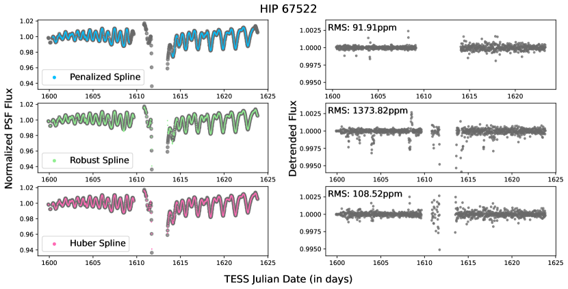
Figure 10: A demonstration of how different splines detrend the light curve of HIP 67522. As can be seen by the low RMS, the penalized spline does a superior job of matching the stellar variability trend and detrending the light curve.

Appendix B Recovery of Known Planets

The following plots depict the recovery of the known young transiting planets using pterodactyls:

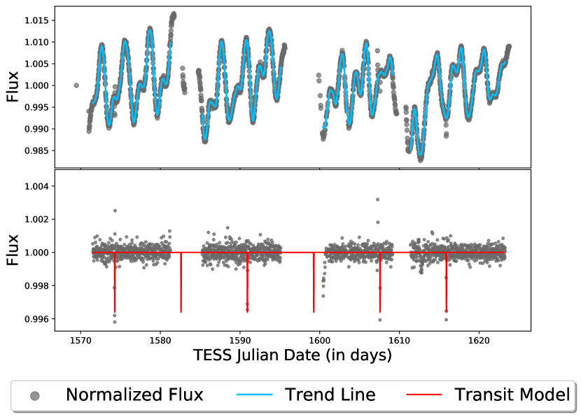
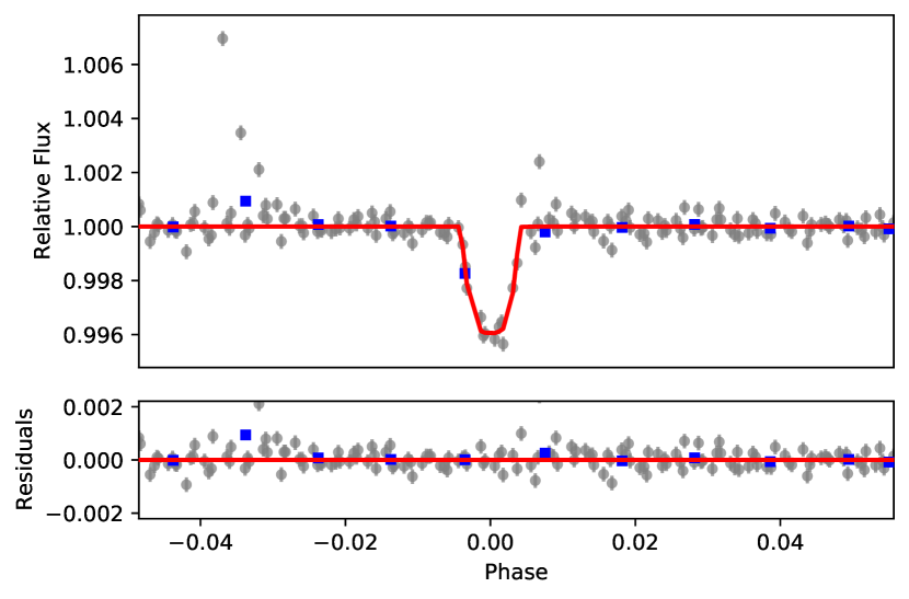
Figure 12: Left: Recovery of TIC 460205581 b. Upper panel: PSF flux (in dark gray) and penalized spline trend (in blue). Lower panel: Detrended light curve (PSF flux divided by the trend). The multi-transit signature (in red) can be clearly seen. Right: Upper panel shows Phase-folded light curve of TIC 460205581 b (gray data points) along with the best fit model using EXOTIC (in red). Lower panel shows the residuals in parts per million.

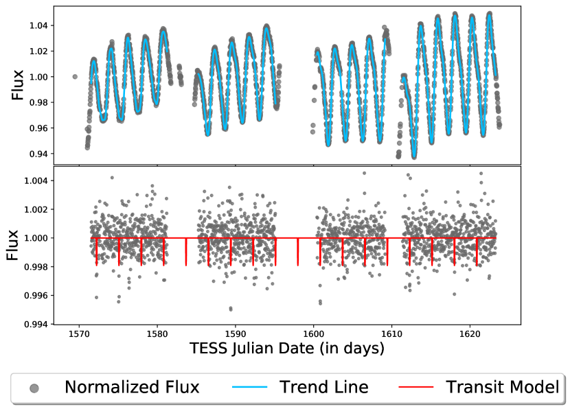
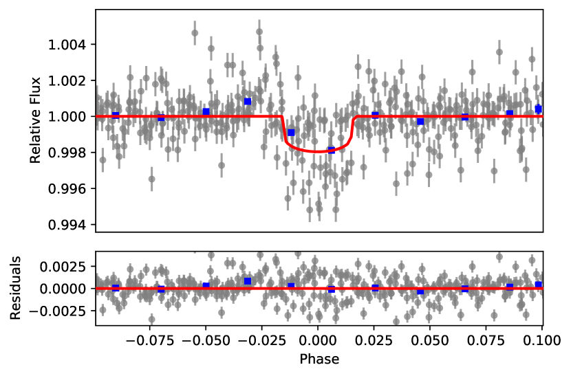
Figure 13: Left: Recovery of TOI 837 b. Upper panel: PSF flux (in dark gray) and penalized spline trend (in blue). Lower panel: Detrended light curve (PSF flux divided by the trend). The multi-transit signature (in red) can be clearly seen. Right: Upper panel shows Phase-folded light curve of TOI 837 b (gray data points) along with the best fit model using EXOTIC (in red). Lower panel shows the residuals in parts per million.

Appendix C Centroid Test

C.1 Recovered Known Transiting Planets

The following plots show the results of the centroid tests for the recovered, known, young transiting planets using pterodactyls. We find that, in all cases, no significant offset was detected i.e., the transiting signal was indeed coming from the target star.

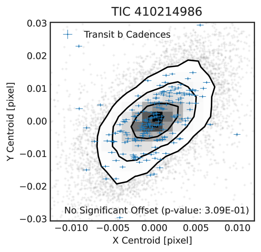
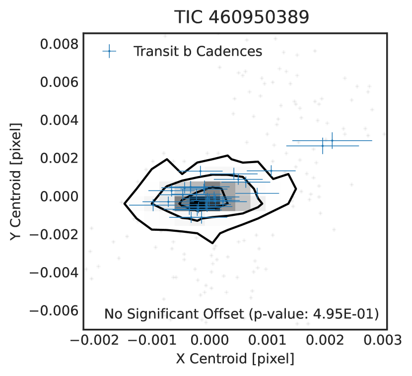
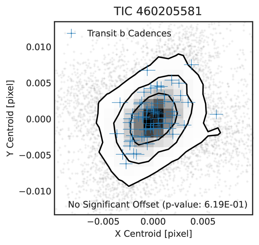
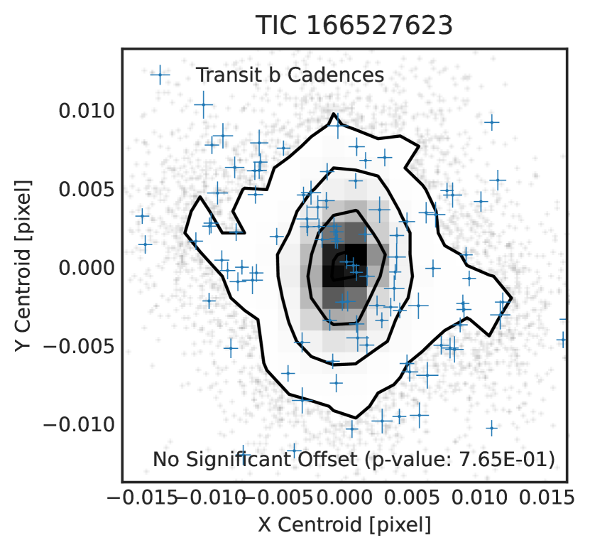
Figure 17: Centroid tests for single planet systems

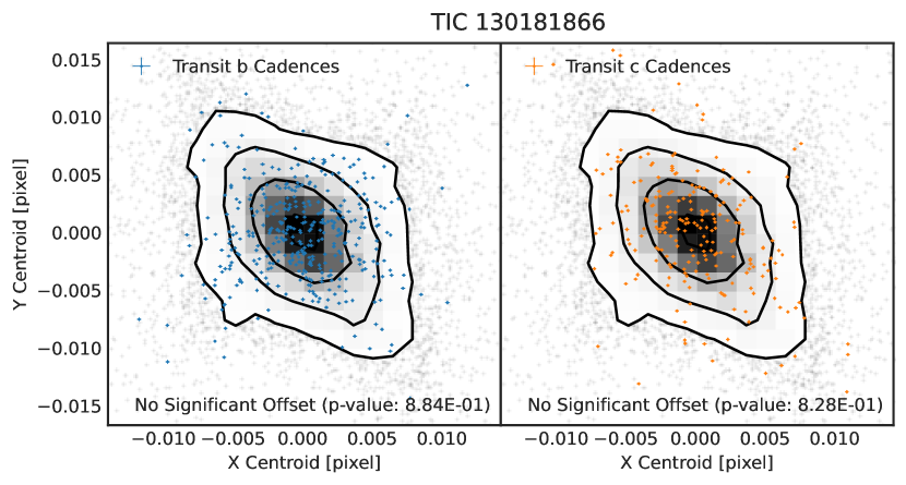
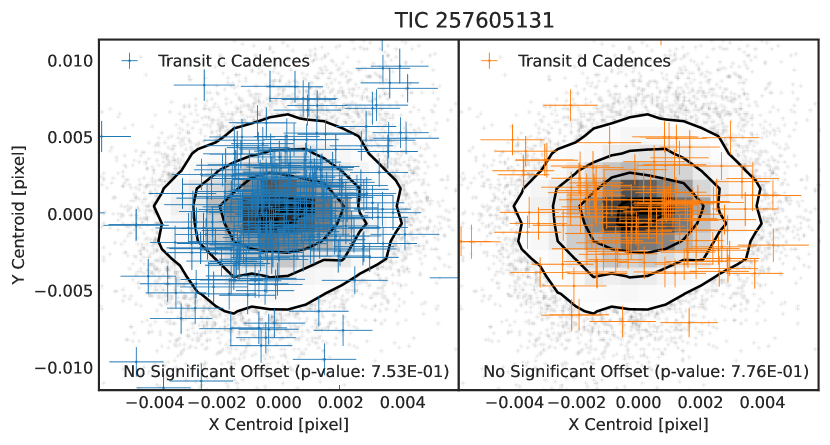
Figure 18: Centroid tests for multi-planet systems

C.2 POIs/Potential Binaries

Hedges (2021) uses the TESS Target Pixel File (TPF; and the aperture information therein) in order to conduct the centroid test. However, TPFs were only available for three of the potential binaries (all of the ones in UCL; shown below) in Table 3 but not for the 12 other candidates (IC2602). As such, we were only able to use this test when the TPF was available. As can be seen below in two of the cases, we see no significant offsets. However, in the case of TIC 177631209, an offset is detected which is consistent with triceratops’ Flat prior prediction i.e., the transiting signal is actually coming from a nearby/background star.

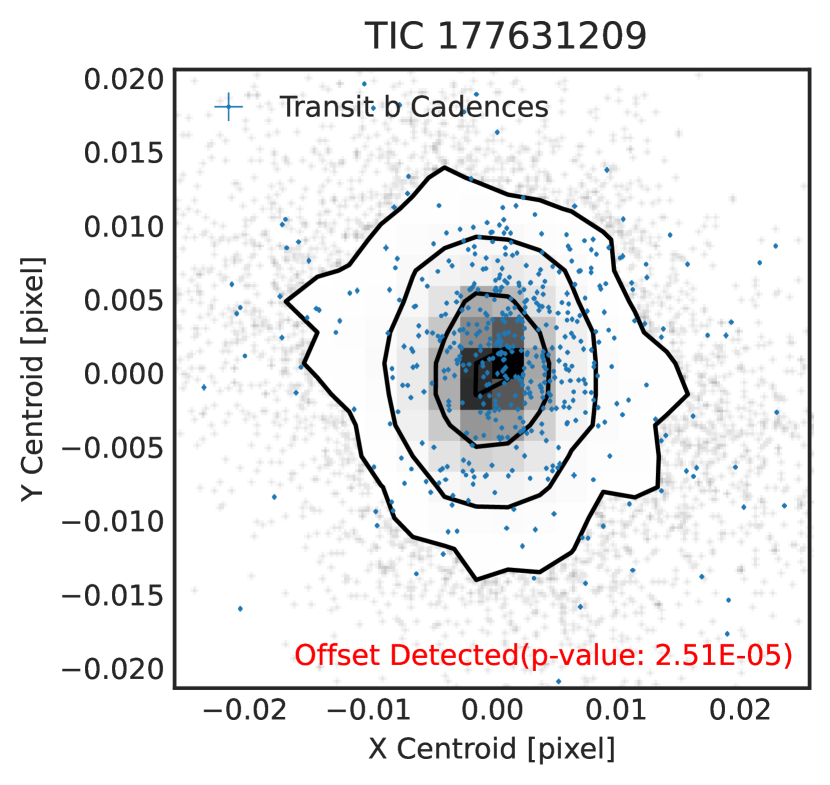
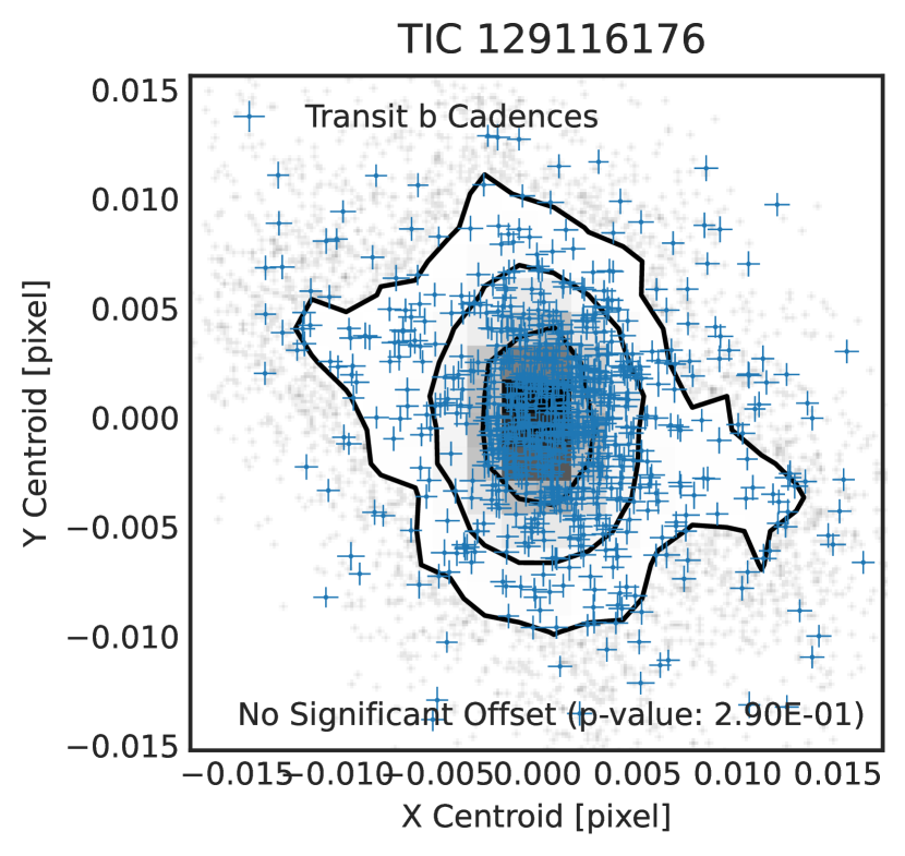
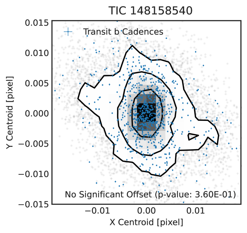
Figure 19: Centroid tests for POIs/Potential Binaries in UCL

Appendix D TESS Input Catalog (TIC) IDs of Cluster Members Searched in this work

D.1 Tucana Horologium Association (THA)

290496318, 266997586, 355766445, 425934574, 281461138, 231867117, 231907973, 231910539, 231914259, 271503441, 234495456, 394210384, 234506344, 234506911, 237880881, 237883772, 237885807, 237910557, 232073492, 234333175, 234338669, 238876720, 274017928, 220523369, 394355443, 238194430, 238196350, 25118964, 33864387, 33881250, 294754396, 319289907, 179315999, 149351776, 141423634, 270623499, 350712873, 150068381, 280865190, 410421717, 79403675, 259845346, 316854083, 406277015, 139984208, 238815210, 327667965, 71274771, 403237836, 234284556, 317016534, 273416539, 197960398, 261560580, 293507177, 229807000, 229807051, 410213494, 410214984, 410214986, 350215424, 325220989, 234290432, 201226029, 325525541, 650381163, 2054867096, 120462356, 12509218, 116157661, 156002545, 117874958, 117874959, 281670243, 206592394, 41862041, 158595208, 206623351, 230982053, 231005004, 229142539, 231020924, 231020638, 219993473, 219998026, 231064749, 231064750, 201753428, 201795667, 201861769, 166787846, 166852312, 166852313, 201898220, 201919099, 201938513, 207138379, 339607562, 381949410, 175298549, 149838027, 224276435, 40059734, 67630561, 140460192, 266746662, 77111651, 152970890, 200790343, 200790342, 401913214, 79566479, 219229275, 219257563, 259542669, 220437346, 381003375, 318785502, 318841562, 141306513, 165184400, 49906916, 176852917, 160008866, 308305105, 93122097, 144653213, 321100028, 44793998, 44794000, 152505948, 170673573, 77339881, 259573397, 161576005, 235056185, 685945639, 632601393, 70596114, 178857861, 117748478, 178969585, 178969584, 406498177, 188969241, 188969240, 77959676, 220622233, 738102496, 397231463, 317325489, 369862028, 451535889, 276967501, 401820403, 401820823, 411956826, 339397736, 466265409, 219953459, 360912453, 265332355, 372106647

D.2 IC 2602

269788982, 270294307, 373886624, 374507880, 374434502, 376150973, 376248958, 376731139, 377487978, 463722209, 463914418, 280562557, 281404104, 295146126, 296056755, 303021887, 303938254, 315312718, 315556844, 316108752, 316657304, 338027557, 338153421, 338155185, 344331260, 344500353, 344748662, 371442380, 372091372, 372598349, 372810731, 374748039, 375211992, 375586505, 375590099, 376026697, 376346464, 376802322, 376802477, 377369998, 377370859, 377954373, 378030265, 378229702, 378229708, 378412167, 378421253, 378503608, 378611172, 378968986, 378971350, 389925947, 389927730, 389987955, 389989102, 389989103, 389992758, 389994091, 390287165, 390297263, 390297906, 390356253, 390358373, 390358936, 390359665, 390359863, 390362683, 390362687, 390364291, 390365611, 390366165, 390366768, 390369742, 390370044, 390440616, 390442052, 390442224, 390442286, 390442621, 390443919, 390444472, 390446082, 390756608, 390757974, 390759555, 390759810, 390759889, 390760156, 390760423, 390840249, 390840539, 390841015, 390842457, 390847186, 390849159, 390850870, 390852244, 390853511, 390853705, 390953365, 390953417, 390954082, 390954865, 390955053, 390965584, 390966887, 390967697, 391166737, 391169363, 391247092, 391248084, 391251375, 391252554, 391333587, 391333777, 391334152, 391336297, 391336489, 391341577, 391345891, 391420878, 391421013, 391421894, 391422697, 391423247, 391423941, 391426350, 391426355, 391426724, 391742621, 391742931, 391798710, 391800466, 397179567, 397256049, 397451050, 397607720, 397608769, 397735761, 397781652, 397786354, 398002694, 398003321, 398007252, 398007510, 398009616, 398497171, 398859114, 398913671, 398919018, 398919062, 400066956, 400326671, 401066440, 401885249, 402190411, 402197704, 453950110, 460019760, 460042206, 460042668, 460044249, 460052791, 460053781, 460071039, 460169886, 460179837, 460205515, 460205581, 460205610, 460205613, 460209001, 460228276, 460230188, 460235527, 460297171, 460335450, 460336403, 460337200, 460338822, 460364093, 460366104, 460451570, 460473652, 460474388, 460493086, 460496906, 460500756, 460500920, 460501099, 460502873, 460526824, 460527147, 460613215, 460623602, 460625223, 460648865, 460649476, 460651700, 460651946, 460652126, 460765494, 460771098, 460772349, 460774571, 460774855, 460793411, 460793464, 460795626, 460796730, 460797477, 460797491, 460803319, 460823191, 460823505, 460825967, 460826876, 460827760, 460835832, 460910972, 460950389, 460950671, 460951259, 460953778, 460957968, 460958645, 460982124, 460982877, 460985868, 461080220, 461117076, 461120837, 461121683, 461123552, 461124617, 461125055, 461125245, 461125565, 461129500, 464897777, 464898410, 464900625, 464901555, 464902649, 464903262, 464905819, 464907721, 464907793, 464925976, 464925998, 464928326, 464928360, 464930364, 464934793, 464935013, 464935253, 464935435, 464936128, 464936356, 464936632, 464937455, 464937480, 464938239, 464969661, 465051041, 465069629, 465071629, 465075473, 465100077, 465104773, 465107223, 465107251, 465107412, 465107540, 465107704, 465109422, 465131523, 465132340, 465250214, 465261021, 465263287, 465264828, 465268721, 465268826, 465271210, 465272595, 465273919, 465275413, 465296988, 465297405, 465302289, 465306494, 465451355, 465456282, 465458552, 465459529, 465461596, 465462490, 465466499, 465466759, 465466991, 465470619, 465470793, 465472920, 465512275, 465593684, 465621749, 465661670, 465663582, 465801421, 465801835, 465803266, 465823847, 465828067, 465828262, 465831049, 465865592, 465902398, 465998642, 466002083, 466003005, 466010610, 466030199, 466032289, 466034300, 466035035, 466181275, 466183196, 466186713, 466194095, 466208965, 466209622, 466215841, 466218647, 466368276, 466370148, 466422383, 466568973, 466573354, 466576983, 466577068, 466579089, 466593335, 466617413, 466617428, 466630156, 466705111, 466736533, 466794262, 466831513, 466953672, 466982490, 467136716, 467138305, 467162035, 467170455, 467232072, 467342418, 467349410, 467351743, 467557909, 467739360, 467953288, 467976475, 467980197, 468093585, 468172174, 468205592, 844245965, 844522717, 847701323, 847769574, 848933728, 849260294, 850363872, 850582149, 850582150, 911292786, 911713906, 911870847, 911870867, 911872987, 911894290, 911920053, 911976941, 912047875, 912047923, 912058973, 913701079, 913996012, 914038861, 915086533, 923545851, 374517370, 374930544, 375679671, 376420337

D.3 Upper Centaurus Lupus (UCL)

410464477, 231813631, 436248798, 157209108, 284422031, 60024614, 53369126, 140295287, 45688827, 280207697, 446764692, 188084200, 48781344, 49046625, 448474635, 178659732, 29982064, 333734230, 437266963, 847323329, 872689258, 73650567, 73710370, 103625477, 124286087, 124512998, 124515557, 134976179, 142391542, 144609763, 144678969, 144921815, 152484504, 152484511, 162093865, 162208214, 178759525, 181229149, 248078069, 301219220, 323245745, 333832656, 390009811, 451452509, 452419080, 461125552, 911963409, 940640910, 998337743, 998337745, 388237166, 454856551, 273349137, 361818250, 258588387, 442062521, 287670422, 245298317, 339301537, 245430125, 363781484, 275705109, 438586540, 438692318, 243164696, 243237647, 165729961, 165775281, 243321910, 165823257, 243330489, 243344284, 243341756, 101940827, 243389982, 243390044, 243393076, 243396962, 243412695, 243427058, 243430178, 243477650, 243496587, 243511069, 241511379, 241511375, 30067072, 241570607, 241573601, 243618821, 207786920, 166447153, 243642384, 243647020, 241640242, 166577188, 241677723, 276004385, 241685708, 111947267, 307143242, 241739877, 113350106, 113277027, 166843863, 420522238, 359830202, 178931743, 359762838, 112176566, 178936965, 261389834, 261389883, 242119768, 326467176, 326742300, 242149069, 179099805, 179130687, 312420298, 312512588, 179220045, 396137563, 328700272, 179291515, 328811406, 242267549, 330123048, 329299765, 179367009, 179413040, 179413905, 179538968, 329815628, 210806853, 242336470, 242367242, 179623765, 179623744, 323269451, 242391843, 179743858, 339413946, 330987798, 331335557, 339530484, 179878718, 413285274, 331523868, 179905128, 332012383, 242548962, 179964001, 242557720, 332213483, 414138813, 125757999, 242583230, 242583644, 167480388, 242595135, 242612195, 242610390, 167546864, 420582698, 167596713, 332888505, 167670025, 90800382, 127024985, 167704195, 241827885, 241825308, 127089264, 333544395, 127203998, 264137167, 127249954, 127311608, 127246209, 211517703, 127315102, 290932786, 457557304, 241883618, 127664368, 83863971, 127731749, 392788625, 291909020, 158809330, 127794299, 127861722, 127791732, 392838495, 128079374, 158979332, 128119540, 159043143, 159195919, 289425666, 430829746, 369971171, 128453434, 128622430, 379593781, 460844584, 159376787, 159372538, 159421340, 159428617, 159428519, 383492888, 383582909, 159496289, 129116176, 129117325, 129060941, 159537293, 188212197, 188991120, 159752939, 383632304, 159754676, 47752102, 129419398, 47828022, 81003, 47884213, 250091359, 129623324, 366011440, 366011855, 250123846, 160089427, 48064387, 129774131, 129948345, 455309397, 160444470, 160404487, 160444291, 455375884, 455410480, 48364505, 160502580, 160504689, 48437482, 309456404, 164844, 160695823, 307425592, 333651699, 440863421, 276130740, 276219648, 121094784, 121102482, 461663855, 35001854, 440880146, 121240521, 121196226, 334129050, 121250827, 334425144, 334424163, 334417833, 121407551, 75543709, 75540884, 334648804, 75616091, 334835256, 75642561, 75648725, 335146096, 335139519, 75735567, 370476997, 121779963, 121779961, 121726626, 335454137, 121839093, 75869475, 335643748, 121982262, 121981993, 75873633, 75931110, 121983359, 121979152, 75933042, 75970186, 75971901, 61012630, 61079477, 160417350, 160417246, 160549804, 76050403, 122083452, 122162363, 76057224, 160633268, 160701354, 160704414, 122244909, 160632970, 160703925, 122250596, 160703933, 121850125, 122288890, 122397232, 122394390, 122397233, 76322064, 76397021, 276293815, 371122327, 276300910, 76435066, 276452267, 276491524, 276503464, 76580025, 141662588, 76587359, 307526685, 307533179, 61530691, 76652075, 142513032, 143414073, 76706808, 76706801, 272341056, 148087359, 148158374, 148158540, 272397344, 272395377, 148158169, 48630780, 272396062, 148261121, 272456799, 272462967, 460329848, 460323913, 225797367, 148480904, 148494823, 225957292, 148495018, 89026796, 148772375, 54172975, 54175032, 54175033, 148904033, 292265209, 292364079, 148904850, 148904891, 54245747, 54449487, 185053184, 54667962, 54810190, 54811378, 1037289516, 976426321, 128116539, 1052698599, 1174609023, 127871423, 42974961, 133010063, 132241629, 149640056, 141045993, 413145172, 461728725, 413693742, 413693728, 414077635, 152377452, 153079294, 149437620, 153781478, 154438290, 155430355, 170986304, 289877522, 172608950, 172608996, 189421351, 172615355, 173560788, 173560502, 173871956, 254322223, 254365686, 254406143, 254387071, 190372855, 176463845, 254451455, 98761335, 98909539, 177342508, 177336303, 177631209, 254597659, 99039745, 99039926, 178201756, 99041233, 99039843, 266271836, 99039842, 99046173, 99046104, 362351038, 254628801, 99205053, 178456568, 269155561, 269155560, 179051609, 179051461, 270107026, 99324522, 179622269, 272977820, 254740868, 254771390, 442611273, 295901750, 295905052, 295899674, 254844960, 295911223, 277674241, 296039638, 442642949, 254930869, 254901458, 296483317, 296700769, 255092900, 58413338, 442813719, 301036163, 301087756, 301048970, 255134616, 442828160, 58583881, 364200069, 364200072, 364200513, 255263576, 255236579, 58751944, 255246336, 292566342, 386943436, 58752825, 58749494, 386980599, 58832313, 294993587, 281164246, 281164807, 279883855, 255403319, 279819212, 279821618, 255407474, 59017926, 59095543, 59095516, 59183599, 59232730, 255464386, 59334299, 93457683, 93456758, 275018323, 255475779, 59403154, 59336031, 59504074, 59500324, 93610654, 93700013, 93779101, 93778206, 69283667, 69377602, 69178294, 256902444, 69420071, 93932740, 214870481, 93985722, 69514028, 69609942, 94159843, 161786522, 161873315, 70041394, 374542527, 374648559, 94491270, 374823554, 374812449, 374719920, 215392772, 374732772, 94731904, 94683443, 457995946, 457993297, 67978974, 382643945, 163141448, 382799779, 382794993, 382870216, 382800509, 382800518, 462044648, 462077825, 462083149, 462147302, 462148256, 462146157, 462147898, 462146834, 68256179, 164029492, 95468062, 382549695, 303188383, 164707310, 303188775, 68416596, 164707361, 318027415, 318030913, 317906231, 318035342, 68565222, 3084844, 410857373, 364368528, 364523302, 96552404, 318141346, 318141352, 96631952, 210541258, 210577071, 221355243, 3926262, 4061225, 222835418, 210908741, 210908710, 222940415, 392328254, 350869718, 210975114, 2743109, 211086449, 224004929, 351521484, 211143017, 211237627, 211237621, 225109252, 352162554, 211459804, 323187268, 211609345, 211681133, 291866634, 280474618, 292925229, 280828479, 280822724, 212201942, 382951562, 205461071, 83687552, 310053760, 458058639, 94972416, 233981889, 397712527, 234869424, 78981730, 79358659, 245927009, 245934292, 337243296, 338104678, 338105219, 246664608, 338495232, 34404183, 339989392, 247348620, 343976519, 212461524, 377523286, 378094374, 381441805, 381441323, 44207349, 193169513, 194744695, 160689461, 17509396, 1232119536, 1233589158, 1336147896, 1343250594, 1160500678, 1247277024, 504761559, 1170473308, 1172055696, 1255305471, 446547327, 469811127, 148910632, 97044158, 285117481, 393808105

D.4 Ursa Major (UMa)

11895653, 224288693, 224292240, 316331312, 224305606, 99381773, 229534764, 1001230963, 157272202, 159190005, 159191044, 141821609, 150387644, 142277151, 159189482, 416538839

D.5 Pisces-Eridani (PiEri)

80363380, 41858251, 262531383, 12787754, 399570739, 240720758, 4579839, 188627184, 311085703, 8938429, 66437682, 66471572, 89526411, 228383334, 89547213, 89547209, 114749459, 37763129, 212963433, 382306185, 28077586, 28092085, 248349830, 67643537, 248384545, 248952247, 70490059, 257434109, 29848163, 404467056, 164777021, 33625968, 423750380, 423750384, 257483561, 257484419, 72729895, 139526229, 120888774, 175491080, 144110354, 630138333, 332714671, 332740776, 270432631, 1028816, 332825272, 332862003, 332864335, 420000810, 1122408, 251064437, 251081955, 64008790, 251088243, 4741056, 65346691, 425095257, 35745429, 35841788, 204613238, 204613241, 141287580, 98855268, 365332374, 23193695, 9805084, 274037216, 441515106, 92250588, 279068672, 55893164, 9967295, 423442532, 12546422, 382326499, 12631414, 121006547, 166741952, 325707772, 156460685, 165219666, 279403260, 44647574, 461713170, 178286446, 257605131, 152590946, 170674625, 651901104, 457161840, 38613715, 55406666, 55441489, 34086013, 34147414, 9161614, 34238114, 34267639, 269724428, 332661361, 250133028, 37816550, 37860207, 248613540, 37903382, 37948770, 71089681, 71091056, 248655215, 38049622, 38049612, 38128400, 55935823, 117735557, 117745508, 56000236, 56127663, 146804027, 167485031, 246896530, 316915529, 152439649, 169396430, 169451121, 169529956, 231303250, 188968885, 188987821, 24607967, 442926120, 442926121, 24719594, 442965496, 143353370, 408233707, 437759888, 385141581

References

- Aigrain et al. (2016) Aigrain, S., Parviainen, H., & Pope, B. 2016, Monthly Notices of the Royal Astronomical Society, 459, 2408
- Babusiaux et al. (2018) Babusiaux, C., van Leeuwen, F., Barstow, M., et al. 2018, Astronomy & astrophysics, 616, A10
- Baglin et al. (2006) Baglin, A., Auvergne, M., Boisnard, L., et al. 2006, cosp, 36, 3749
- Beaugé & Nesvorný (2013) Beaugé, C., & Nesvorný, D. 2013, ApJ, 763, 12
- Borucki (2017) Borucki, W. J. 2017, Proceedings of the American Philosophical Society, 161, 38
- Borucki et al. (2010) Borucki, W. J., Koch, D., Basri, G., et al. 2010, Science, 327, 977
- Bouma et al. (2020) Bouma, L., Hartman, J., Brahm, R., et al. 2020, The Astronomical Journal, 160, 239
- Buchner (2021) Buchner, J. 2021, arXiv preprint arXiv:2101.09604
- Chen & Kipping (2017) Chen, J., & Kipping, D. 2017, ApJ, 834, 17
- Ciardi et al. (2018) Ciardi, D. R., Crossfield, I. J. M., Feinstein, A. D., et al. 2018, AJ, 155, 10
- David et al. (2019) David, T. J., Petigura, E. A., Luger, R., et al. 2019, The Astrophysical Journal Letters, 885, L12
- Dong & Zhu (2013) Dong, S., & Zhu, Z. 2013, The Astrophysical Journal, 778, 53
- Dressing & Charbonneau (2015) Dressing, C. D., & Charbonneau, D. 2015, The Astrophysical Journal, 807, 45
- Eilers & Marx (1996) Eilers, P. H., & Marx, B. D. 1996, Statistical science, 89
- Feinstein et al. (2019) Feinstein, A. D., Montet, B. T., Foreman-Mackey, D., et al. 2019, Publications of the Astronomical Society of the Pacific, 131, 094502
- Feliz et al. (2021) Feliz, D. L., Plavchan, P., Bianco, S. N., et al. 2021, arXiv preprint arXiv:2103.05647
- Fernandes et al. (2019) Fernandes, R. B., Mulders, G. D., Pascucci, I., Mordasini, C., & Emsenhuber, A. 2019, The Astrophysical Journal, 874, 81
- Feroz & Hobson (2008) Feroz, F., & Hobson, M. P. 2008, MNRAS, 384, 449
- Fulton et al. (2017) Fulton, B. J., Petigura, E. A., Howard, A. W., et al. 2017, The Astronomical Journal, 154, 109
- Gagné et al. (2018) Gagné, J., Mamajek, E. E., Malo, L., et al. 2018, The Astrophysical Journal, 856, 23
- Gaia Collaboration et al. (2018) Gaia Collaboration, Brown, A. G. A., Vallenari, A., et al. 2018, A&A, 616, A1
- Gaidos et al. (2017) Gaidos, E., Mann, A., Rizzuto, A., et al. 2017, Monthly Notices of the Royal Astronomical Society, 464, 850
- Giacalone et al. (2021) Giacalone, S., Dressing, C. D., Jensen, E. L. N., et al. 2021, AJ, 161, 24
- Ginzburg et al. (2016) Ginzburg, S., Schlichting, H. E., & Sari, R. 2016, The Astrophysical Journal, 825, 29
- Ginzburg et al. (2018) —. 2018, Monthly Notices of the Royal Astronomical Society, 476, 759
- Gupta & Schlichting (2019) Gupta, A., & Schlichting, H. E. 2019, Monthly Notices of the Royal Astronomical Society, 487, 24
- Gupta & Schlichting (2020) Gupta, A., & Schlichting, H. E. 2020, MNRAS, 493, 792
- Hardegree-Ullman et al. (2020) Hardegree-Ullman, K. K., Zink, J. K., Christiansen, J. L., et al. 2020, The Astrophysical Journal Supplement Series, 247, 28
- Hedges (2021) Hedges, C. 2021, Research Notes of the AAS, 5, 262
- Henry et al. (2006) Henry, T. J., Jao, W.-C., Subasavage, J. P., et al. 2006, The Astronomical Journal, 132, 2360
- Hippke et al. (2019) Hippke, M., David, T. J., Mulders, G. D., & Heller, R. 2019, The Astronomical Journal, 158, 143
- Hippke & Heller (2019) Hippke, M., & Heller, R. 2019, Astronomy & Astrophysics, 623, A39
- Howard et al. (2012) Howard, A. W., Marcy, G. W., Bryson, S. T., et al. 2012, The Astrophysical Journal Supplement Series, 201, 15
- Howell et al. (2014) Howell, S. B., Sobeck, C., Haas, M., et al. 2014, Publications of the Astronomical Society of the Pacific, 126, 398
- Huang et al. (2020a) Huang, C. X., Vanderburg, A., Pál, A., et al. 2020a, Research Notes of the AAS, 4, 204
- Huang et al. (2020b) —. 2020b, Research Notes of the AAS, 4, 206
- Huber (1981) Huber, P. 1981, Robust Statistics, Wiley Series in Probability and Statistics (Wiley)
- Hunter (2007) Hunter, J. D. 2007, Computing in Science & Engineering, 9, 90
- Johnson et al. (2017) Johnson, J. A., Petigura, E. A., Fulton, B. J., et al. 2017, The Astronomical Journal, 154, 108
- Jones et al. (2001–) Jones, E., Oliphant, T., Peterson, P., et al. 2001–, SciPy: Open source scientific tools for Python, [Online; accessed ¡today¿]
- Kopparapu et al. (2018) Kopparapu, R. K., Hébrard, E., Belikov, R., et al. 2018, The Astrophysical Journal, 856, 122
- Kovács et al. (2002) Kovács, G., Zucker, S., & Mazeh, T. 2002, Astronomy & Astrophysics, 391, 369
- Kreidberg (2015) Kreidberg, L. 2015, Publications of the Astronomical Society of the Pacific, 127, 1161
- Kunimoto et al. (2021) Kunimoto, M., Huang, C., Tey, E., et al. 2021, Research Notes of the AAS, 5, 234
- Livingston et al. (2018) Livingston, J. H., Crossfield, I. J., Petigura, E. A., et al. 2018, The Astronomical Journal, 156, 277
- Lomb (1976) Lomb, N. R. 1976, Astrophysics and space science, 39, 447
- Mandel & Agol (2002) Mandel, K., & Agol, E. 2002, The Astrophysical Journal Letters, 580, L171
- Manduca et al. (1977) Manduca, A., Bell, R., & Gustafsson, B. 1977, Astronomy and Astrophysics, 61, 809
- Mann et al. (2016a) Mann, A. W., Gaidos, E., Mace, G. N., et al. 2016a, The Astrophysical Journal, 818, 46
- Mann et al. (2016b) Mann, A. W., Newton, E. R., Rizzuto, A. C., et al. 2016b, The Astronomical Journal, 152, 61
- Mann et al. (2017) Mann, A. W., Vanderburg, A., Rizzuto, A. C., et al. 2017, The Astronomical Journal, 155, 4
- Mann et al. (2020) Mann, A. W., Johnson, M. C., Vanderburg, A., et al. 2020, The Astronomical Journal, 160, 179
- Meibom et al. (2011) Meibom, S., Barnes, S. A., Latham, D. W., et al. 2011, The Astrophysical Journal Letters, 733, L9
- Meibom et al. (2013) Meibom, S., Torres, G., Fressin, F., et al. 2013, Nature, 499, 55
- Mulders et al. (2019) Mulders, G. D., Mordasini, C., Pascucci, I., et al. 2019, ApJ, 887, 157
- Mulders et al. (2020) Mulders, G. D., O’Brien, D. P., Ciesla, F. J., Apai, D., & Pascucci, I. 2020, The Astrophysical Journal, 897, 72
- Mulders et al. (2015) Mulders, G. D., Pascucci, I., & Apai, D. 2015, ApJ, 814, 130
- Mulders et al. (2015) Mulders, G. D., Pascucci, I., & Apai, D. 2015, The Astrophysical Journal, 798, 112
- Mulders et al. (2018) Mulders, G. D., Pascucci, I., Apai, D., & Ciesla, F. J. 2018, The Astronomical Journal, 156, 24
- Mulders et al. (2018) Mulders, G. D., Pascucci, I., Apai, D., & Ciesla, F. J. 2018, AJ, 156, 24
- Mullally et al. (2016) Mullally, F., Coughlin, J. L., Thompson, S. E., et al. 2016, Publications of the Astronomical Society of the Pacific, 128, 074502
- Nardiello et al. (2020) Nardiello, D., Piotto, G., Deleuil, M., et al. 2020, Monthly Notices of the Royal Astronomical Society, 495, 4924
- Newton et al. (2019) Newton, E. R., Mann, A. W., Tofflemire, B. M., et al. 2019, The Astrophysical Journal Letters, 880, L17
- Newton et al. (2021) Newton, E. R., Mann, A. W., Kraus, A. L., et al. 2021, The Astronomical Journal, 161, 65
- Ofir (2014) Ofir, A. 2014, Astronomy & Astrophysics, 561, A138
- Owen & Wu (2013) Owen, J. E., & Wu, Y. 2013, The Astrophysical Journal, 775, 105
- Owen & Wu (2017) —. 2017, The Astrophysical Journal, 847, 29
- Pascucci et al. (2018) Pascucci, I., Mulders, G. D., Gould, A., & Fernand es, R. 2018, ApJ, 856, L28
- Pascucci et al. (2019) Pascucci, I., Mulders, G. D., & Lopez, E. 2019, ApJ, 883, L15
- Pearson (2019) Pearson, K. A. 2019, AJ, 158, 243
- Pearson et al. (2019) Pearson, K. A., Griffith, C. A., Zellem, R. T., Koskinen, T. T., & Roudier, G. M. 2019, AJ, 157, 21
- Pearson et al. (2018) Pearson, K. A., Palafox, L., & Griffith, C. A. 2018, MNRAS, 474, 478
- Petigura et al. (2013) Petigura, E. A., Howard, A. W., & Marcy, G. W. 2013, Proceedings of the National Academy of Sciences, 110, 19273
- Petigura et al. (2017) Petigura, E. A., Howard, A. W., Marcy, G. W., et al. 2017, The Astronomical Journal, 154, 107
- Petigura et al. (2018) Petigura, E. A., Marcy, G. W., Winn, J. N., et al. 2018, The Astronomical Journal, 155, 89
- Pope et al. (2016) Pope, B. J., Parviainen, H., & Aigrain, S. 2016, Monthly Notices of the Royal Astronomical Society, 461, 3399
- Rebull et al. (2016) Rebull, L. M., Stauffer, J. R., Bouvier, J., et al. 2016, AJ, 152, 114
- Ricker et al. (2014) Ricker, G. R., Winn, J. N., Vanderspek, R., et al. 2014, Journal of Astronomical Telescopes, Instruments, and Systems, 1, 014003
- Rizzuto et al. (2017) Rizzuto, A. C., Mann, A. W., Vanderburg, A., Kraus, A. L., & Covey, K. R. 2017, The Astronomical Journal, 154, 224
- Rizzuto et al. (2018) Rizzuto, A. C., Vanderburg, A., Mann, A. W., et al. 2018, The Astronomical Journal, 156, 195
- Rizzuto et al. (2020) Rizzuto, A. C., Newton, E. R., Mann, A. W., et al. 2020, The Astronomical Journal, 160, 33
- Savitzky & Golay (1964) Savitzky, A., & Golay, M. J. 1964, Analytical chemistry, 36, 1627
- Scargle (1982) Scargle, J. D. 1982, The Astrophysical Journal, 263, 835
- Shporer et al. (2017) Shporer, A., Zhou, G., Vanderburg, A., et al. 2017, The Astrophysical Journal Letters, 847, L18
- Siverd et al. (2012) Siverd, R. J., Beatty, T. G., Pepper, J., et al. 2012, The Astrophysical Journal, 761, 123
- Skilling (2004) Skilling, J. 2004, in American Institute of Physics Conference Series, Vol. 735, American Institute of Physics Conference Series, ed. R. Fischer, R. Preuss, & U. V. Toussaint, 395–405
- Stassun et al. (2018) Stassun, K. G., Oelkers, R. J., Pepper, J., et al. 2018, The Astronomical Journal, 156, 102
- Thompson et al. (2018) Thompson, S. E., Coughlin, J. L., Hoffman, K., et al. 2018, The Astrophysical Journal Supplement Series, 235, 38
- van der Walt et al. (2011) van der Walt, S., Colbert, S. C., & Varoquaux, G. 2011, Computing in Science & Engineering, 13, 22
- Vanderburg et al. (2018) Vanderburg, A., Mann, A. W., Rizzuto, A., et al. 2018, The Astronomical Journal, 156, 46
- Werner et al. (2004) Werner, M. W., Roellig, T., Low, F., et al. 2004, The Astrophysical Journal Supplement Series, 154, 1
- Winters et al. (2014) Winters, J. G., Henry, T. J., Lurie, J. C., et al. 2014, The Astronomical Journal, 149, 5
- Zellem et al. (2020) Zellem, R. T., Pearson, K. A., Blaser, E., et al. 2020, Publications of the Astronomical Society of the Pacific, 132, 054401
- Zink (2019) Zink, J. 2019, jonzink/EDI-Vetter: Initial Release, doi:10.5281/zenodo.3585940
- Zink et al. (2020) Zink, J. K., Hardegree-Ullman, K. K., Christiansen, J. L., et al. 2020, The Astronomical Journal, 159, 154