Simultaneous J-, H-, K- and L-band spectroscopic observations of galactic Be stars

Abstract

Context. It is already accepted that Be stars are surrounded by circumstellar envelopes, which are mostly compatible with a disc geometry in Keplerian rotation. Their infrared region is characterised by a moderate flux excess and the presence of hydrogen recombination lines that allow us to obtain information on the physical and dynamical structure of different regions inside the disc. Nevertheless, many of the infrared studies available in the literature show low-resolution spectra, or are restricted to a small object sample or describe just an individual object. Some others analyse reduced spectral ranges or just one infrared band.

Aims. We aim to obtain a more complete characterisation of the properties of the circumstellar environment of Be stars that helps to constrain the theoretical models of the Be phenomenon.

Methods. Throughout the last decade, we used the spectroscopic facilities at the Gemini and Las Campanas observatories to obtain quasi-simultaneous spectra in the J, H, K, and L bands of a sample of Be stars with medium resolution.

Results. We present near-infrared, medium-resolution spectra of a sample of galactic Be stars with different spectral subtypes and luminosity classes. We measure different parameters of the hydrogen recombination lines from the Paschen, Brackett, Pfund, and Humphreys series, and use them to diagnose physical conditions in the circumstellar environment. We analysed the equivalent-width (EW) ratio between Br$\alpha$ and Br$\gamma$ lines and different diagrams of flux ratios. We also identify lines from He i, C i, N i, O i, Na i, Mg i, Mg ii, Si i, Fe i, and Fe ii. Analysing the EW measurements of particular He i, Mg ii, Fe i, Fe ii and O i lines, we find that for some lines they correlate with the spectral type of the star. Particularly, the emission of the O i $\lambda\,1.3168\,\mu$m line decreases towards the later spectral types.

Conclusions. We present an atlas of 22 Be stars, that covers a wide infrared (IR) spectral range with quasi-simultaneous observations. From a detailed analysis, we define new complementary criteria to Mennickent’s classification of Be stars according to their disc opacity. Some objects in our sample present compact thick envelopes, while in others the envelope is extended and optically thin. The correlation between the full widths at half maximum (FWHM) and the peak separation ($\Delta\mathrm{V}$) versus $V\,\sin\,i$ for the Br10, Br$\delta$, and Hu14 lines reveals that the broadening mechanism is rotational. The Ly$\beta$ fluorescence is a key mechanism to explain the intensity of the emission of Mg ii and O i lines.

1 Introduction

Be stars are rapidly rotating, non-supergiant B-type stars, whose spectra show or have shown the H$\alpha$ line in emission (Jaschek et al., 1981; Collins, 1987). It is already accepted that these objects present circumstellar envelopes, mostly compatible with a disc geometry in Keplerian rotation (Rivinius et al., 2013). The infrared (IR) part of their spectra is characterised by a moderate flux excess and the presence of numerous hydrogen emission lines of the Paschen, Brackett, Pfund, and Humphreys series. These lines are formed in a region more internal than that of the optical H lines, and, for most of them, the photospheric absorption contribution is negligible (Steele & Clark, 2001; Lenorzer et al., 2002b). Thus, they allow us to obtain information on the physical and dynamical structure of different regions within the disc (Hony et al., 2000; Lenorzer et al., 2002a; Mennickent et al., 2009; Granada et al., 2010; Sabogal et al., 2017).

While different studies devoted to the near-IR spectra of Be stars show low-resolution data, many of them are restricted to a small sample, and some others analyse reduced spectral ranges. For instance, there are only a few studies done in the J band, and they focus mainly on a particular object or a specific spectral line or element (Mathew et al., 2012a, b; Štefl et al., 2009). Also, individual spectral ranges have already been studied for large samples of Be stars. Steele & Clark (2001) presented H-band spectroscopy of Be stars with a spectral resolution of R $\simeq$ 3 000. They reported Brackett and Fe ii lines in emission and, from the analysis of the strength ratio of the higher Brackett lines to Br$\gamma$, were able to distinguish early- from late-type Be stars. Later, Chojnowski et al. (2015) published high-resolution H-band spectroscopy for a great number of Be stars observed with APOGEE. They found that the Br11 emission line is formed preferentially in a circumstellar disc at an average distance of $\sim 2.2\,R_{\star}$, while the higher Brackett lines seem to originate in an innermost region. Several emission lines have been identified for the first time, such as C i $\lambda\,1.6895\,\mu$m, which is also formed in the inner region of the discs. In a later work, Chojnowski et al. (2017) analysed the variation of the emission strength, peak intensity ratio, and peak separation. Their analysis revealed a variety of temporal variability, including the disappearance and appearance of the line emission on different timescales. In the K band, Hanson et al. (1996), Clark & Steele (2000) and Granada et al. (2010) reported Br$\gamma$, Br$\delta$, and Pfund lines in emission together with lines of He i in emission or absorption, and Mg ii, Fe ii and Na i lines in emission. Clark & Steele (2000) related the infrared characteristics to the underlying properties of the stars: objects that present He i features in emission or absorption are B3 or earlier; if the star presents Mg ii in emission but no He i, it is between B2 and B4; objects with Br$\gamma$ emission but no evidence of He i or Mg ii are B5 or later. Lenorzer et al. (2002b) provided an extensive atlas of early type stars, including a number of Be stars, covering the K and L bands, while Lenorzer et al. (2002a) analysed the H recombination lines of those stars and constructed a diagram of flux ratios of some selected recombination lines: Hu14/Br$\alpha$ and Hu14/Pf$\gamma$. In this diagram, the location of the objects gives information about the density of the emitting gas. After that, Mennickent et al. (2009) presented a classification scheme for Be stars based on the intensity of the L-band hydrogen-emission lines. The objects in each group fall in different regions of Lenorzer’s diagram; thus, this classification scheme is probably connected to the density of the disc. Granada et al. (2010) analysed a sample of eight Be stars and classified them with Mennickent’s criterion. They found that for group I objects, the equivalent widths (EW) of Br$\alpha$ and Br$\gamma$ lines are similar, while for stars in group II the EW(Br$\gamma$) is much larger (more than five times) than the EW(Br$\alpha$). Besides this, Mennickent et al. (2009) and Granada et al. (2010) reported emission lines not only in Br$\alpha$, Pf$\gamma$, and the Humphreys series but also in He i $\lambda\,4.038\,\mu$m and He i $\lambda\,4.041\,\mu$m. Sabogal et al. (2017) showed a sample of L-band Be-star spectra and correlated the infrared features with the optical H$\alpha$ line behaviour.

Despite the broad studies performed in the near-IR (NIR) bands, an analysis of Be stars observed (quasi) simultaneously in the whole range ($0.8-4.5\,\mu$m) is still lacking. In order to obtain a more complete picture of the properties of their circumstellar environment, we collected a great number of NIR spectra of Be stars that cover a wider spectral range than those reported in previous works. These spectra together with the results we obtained from them, will be presented in a series of future papers. In this first work we present a medium resolution (R$\sim$1 800 and R$\sim$6 000) spectral atlas of a sample of 22 galactic Be stars, observed quasi-simultaneously in the J, H, K, and L bands. The paper is organised as follows. In Sect. 2 we present the observations. In Sect. 3 we present and describe the spectra and highlight their main features. The discussion is presented in Sect. 4, and our conclusions are in Sect. 5. The circumstellar parameters derived from the lines described here will be presented in the second paper of this series.

2 Observations

Medium-resolution NIR spectra were obtained for 22 galactic Be stars with spectral types in the O7.5-A0 range and different luminosity classes. The objects were selected either due to their reported variability (Hubert & Floquet, 1998; Mennickent et al., 2009; Granada et al., 2010) or the fact that they have envelope sizes determined by interferometric techniques (Cochetti et al., 2019). This allows us to analyse the evolution of the circumstellar envelopes, with the aim of performing a more complete analysis by adding IR spectroscopic observations.

The observed Be stars are listed in Table 1, which provides information about the HD name, alternative name, spectral type (ST), luminosity class (LC), projected rotational velocity ($V\,\sin\,i$), effective temperature (T_eff), and surface gravity ($\log g$).

Table 1: Fundamental parameters for the programme’s Be stars.

HD	Name	ST(a)	LC(a)	$V\,\sin\,i^{(b)}$ [km/s]	T${}_{\mathrm{eff}}^{(b)}$ [K]	$\log g^{(b)}$ [dex]
HD 20336	BK Cam	B2.5	V	341 $\pm$ 23	18684$\pm$517	3.865$\pm$0.072
HD 23862	28 Tau	B8	V	290 $\pm$ 15	12106$\pm$272	3.937$\pm$0.052
HD 25940	48 Per	B3	V	220 $\pm$ 13	16258$\pm$582	3.572$\pm$0.084
HD 28497	228 Eri	B2	V	342 $\pm$ 24	26724$\pm$427	4.200$\pm$0.046
HD 29441	V1150 Tau	B2.5	V	274 $\pm$ 42(c)	18000(g)	3.8(g)
HD 32991	105 Tau	B2	V	175 $\pm$ 18(d)	20900(h)	3.77(h)
HD 35439	$\psi_{01}$ Ori	B1	V	266 $\pm$ 13	22134$\pm$665	3.920$\pm$0.087
HD 36576	120 Tau	B2	IV-V	266 $\pm$ 13	22618$\pm$508	3.804$\pm$0.062
HD 37490	$\omega$ Ori	B3	V	155 $\pm$ 5 (e)	14492(h)	3.86(h)
HD 41335	V696 Mon	B3-5	V	376 $\pm$ 26	20902$\pm$610	3.886$\pm$0.081
HD 68980	MX Pup	B1.5	IV	152 $\pm$ 8	25126$\pm$642	3.951$\pm$0.077
HD 142983	48 Lib	B3 (f)	V (f)	407 $\pm$ 22	17642$\pm$554	3.845$\pm$0.080
HD 155806	V1075 Sco	O7.5	V	105 $\pm$ 16(c)	34000(i)	4.0(i)
HD 164284	66 Oph	B2	V	287 $\pm$ 21	21609$\pm$523	3.943$\pm$0.068
HD 171623	HR 6977	A0	V	253 $\pm$ 38(c)	9853$\pm$291 (j)	3.91$\pm$0.23 (j)
HD 178175	V4024 Sgr	B2	V	111 $\pm$ 7	18939$\pm$286	3.489$\pm$0.035
HD 183656	V923 Aql	B7	III	284 $\pm$ 16	12626$\pm$524	3.295$\pm$0.081
HD 187811	12 Vul	B2.5	V	258 $\pm$ 13	18086$\pm$583	3.810$\pm$0.083
HD 191610	28 Cyg	B2.5	V	318 $\pm$ 22	18353$\pm$516	3.718$\pm$0.072
HD 209409	$o$ Aqr	B7	IV	282 $\pm$ 20	12942$\pm$402	3.701$\pm$0.067
HD 212571	$\pi$ Aqr	B1	III-IV	233 $\pm$ 15	26061$\pm$736	3.915$\pm$0.088
HD 217050	EW Lac	B4	III	355 $\pm$ 25	17893$\pm$509	3.571$\pm$0.070

(a) CDS database, except other source is indicated; (b) Frémat et al. (2005), except other source is indicated; (c) Głȩbocki & Gnaciński (2005); (d) Abt et al. (2002); (e) Chauville et al. (2001); (f) Zorec et al. (2005). (g) using $T_{\text{eff}}$ y $\log g$ from other stars with the same ST; (h) Cochetti et al. (2019); (i) Cox & Pilachowski (2000); (j) Cochetti et al. (2020).

Observations were performed between 2010 and 2017 using Gemini Near-Infrared Spectrograph (GNIRS; Elias et al., 2006a, b), mounted on the Gemini North telescope, under the following programmes: GN-2010B-Q-2, GN-2012B-Q-56, GN-2016B-Q-83, GN-2017A-Q-84, GN-2017A-Q-89, GN-2017B-Q-81, and GN-2017B-Q-86. In Table 2, we describe the instrumental configurations in longslit or cross-dispersed mode that were used. These configurations provide a resolving power of R $\sim$ 1800.

Table 2: Different GNIRS configurations used on each observing run.

Year	Mode	Camera	Disperser	Slit	Bands
2010	LS	short blue (0.15”/pix)	32 l/mm	0.3”	H-K
		short red (0.15”/pix)	32 l/mm	0.3”	L
2012	LS	short blue (0.15”/pix)	32 l/mm	0.3”	H-K
		long red (0.05”/pix)	101 l/mm	0.1”	L
2016/2017	XD	short blue (0.15”/pix)	32 l/mm	0.3”	J-H-K
	LS	long red (0.05”/pix)	10 l/mm	0.1”	L

In addition, in 2017, we performed observations with the Folded-port InfraRed Echellette (FIRE) spectrometer at Las Campanas Observatory (LCO), Chile. FIRE spectra were obtained with the high-resolution echellete mode covering the 0.8-2.5 $\mu$m range with a resolving power of R $\sim 6000$.

For the data obtained in both telescopes, the reduction procedure is similar. Several ABBA sequences were taken for each target. Flats and comparison arc lamps were taken with each source and telluric-standard star pair. We used the IRAF software package tasks to extract and calibrate the GNIRS spectra and the IDL pipeline provided by Las Campanas Observatory to process FIRE observations. Data reduction steps consisted of subtracting of the AB pairs, flat-fielding, telluric-correction and wavelength and flux calibrations.

To perform the telluric and instrumental corrections, we used late-B- or early-A-type telluric standard stars, observed near the object in both time and sky position (air mass). The telluric spectrum was used to divide each programme’s object spectrum to obtain a telluric-corrected one. Correction for telluric lines is often a difficult task, and, in many cases, we were not able to cancel them out completely. Thus, some residuals of the telluric lines remained in a few spectra, especially at the end of each band and particularly around $2\,\mu$m (K band). However, this effect does not significantly affect the profile of the emission lines, except for the weakest ones.

The wavelength calibration was performed using a calibration lamp, except in the case of the L-band spectra, where we used the telluric lines. Because of the small number of telluric lines available in the standard star spectrum that can be used as wavelength reference, some L-band spectra show a less precise wavelength calibration.

To flux-calibrate Gemini spectra, we used the telluric spectra subtracted by the hydrogen absorption lines as flux standards. Finally, the spectra were corrected for heliocentric velocities.

In FIRE spectra there are gaps in the regions between orders; for example, around $2.28\,\mu$m. Table 3 gives the log of the quasi-simultaneous observations, which includes, for each observed Be star, spectrograph, the observing date and observed bands. For the objects for which the time separation between the two observations is longer than ten days, we checked in the BeSS database if the star spectrum showed variations in the optical range between those dates. In all the cases, the H$\alpha$ profile remained very similar.

Table 3: Log of the quasi-simultaneous observations of Be stars in the J, H, K, and L bands.

Name	Spectrograph	Obs. date	Bands
BK Cam	GNIRS	2016-11-16	J	H	K	L
28 Tau	GNIRS	2016-11-16				L
		2016-11-18	J	H	K
48 Per	GNIRS	2013-01-01		H	K	L
228 Eri	GNIRS	2017-12-10	J	H	K
		2017-12-14				L
V1150 Tau	GNIRS	2012-12-23		H	K	L
105 Tau	GNIRS	2017-01-04	J	H	K	L
$\psi_{01}$ Ori	GNIRS	2017-12-14				L
		2018-01-04	J	H	K
120 Tau	GNIRS	2017-12-29	J	H	K
		2018-01-04				L
$\omega$ Ori	GNIRS	2018-01-04	J	H	K	L
V696 Mon	GNIRS	2017-12-29	J	H	K
		2018-01-14				L
MX Pup	FIRE	2017-06-03	J	H	K
48 Lib	GNIRS	2017-07-09	J	H	K
V1075 Sco	FIRE	2017-06-04	J	H	K
66 Oph	GNIRS	2017-07-03	J	H	K	L
HD  171623	FIRE	2017-06-04	J	H	K
V4024 Sgr	FIRE	2017-06-04	J	H	K
V923 Aql	GNIRS	2017-05-29				L
		2017-07-08	J	H	K
12 Vul	GNIRS	2010-09-15		H	K	L
28 Cyg	GNIRS	2017-07-09	J	H	K	L
$o$ Aqr	GNIRS	2017-07-10	J	H	K
EW Lac	GNIRS	2017-12-27				L
		2018-01-11	J	H	K
$\pi$ Aqr	FIRE	2017-06-04	J	H	K
Observations per band			19	22	22	15

3 Results

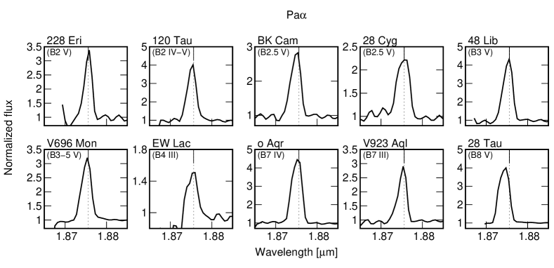
Figure 13: Pa$\alpha$-line profiles.

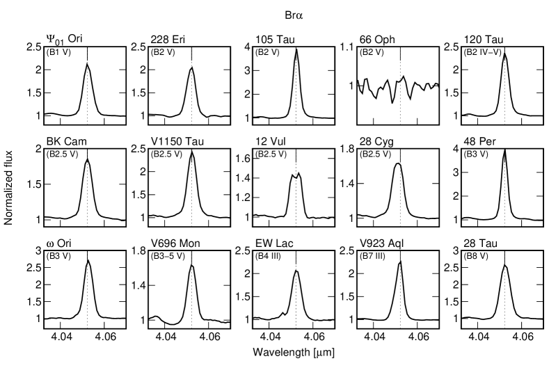
Figure 14: Br$\alpha$-line profiles.

In the following sub-sections, we present and describe the main features that characterise the NIR spectra for the programme’s Be stars. Figures 1,  2, and 9 to  12 show the complete set of spectra, which were normalised and vertically shifted to ease inspection and comparison. The spectra are organised according to the spectral type of the star, and the positions of the identified features are labelled. The spectral regions with telluric residual lines are marked with the $\oplus$ symbol. Figures 13 and 14 present the line profiles of the most intense lines, Pa$\alpha$ and Br$\alpha$, which are overlapped in the complete spectra figures.

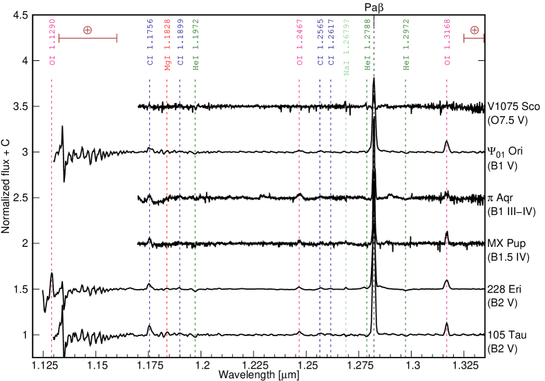
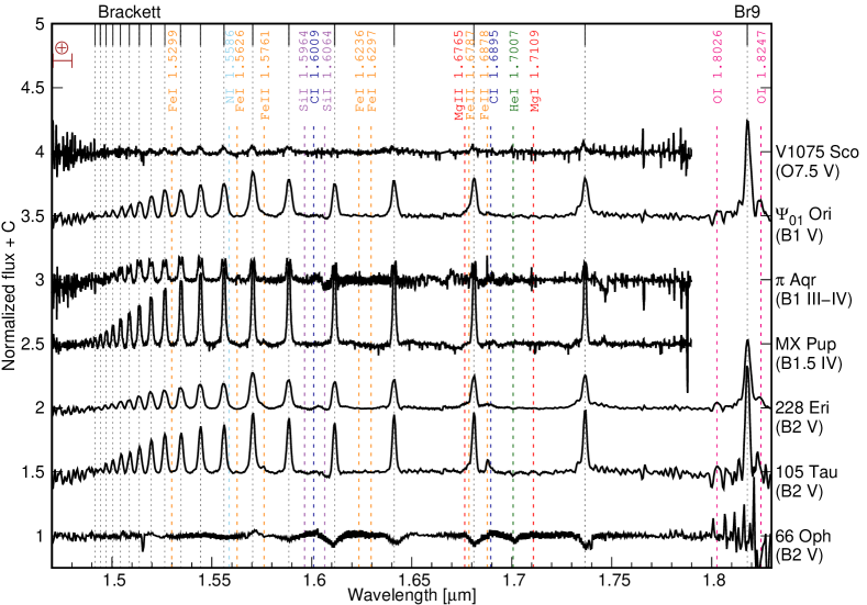
Figure 1: J- (upper panel) and H-band (lower panel) spectra of Be stars. Spectra are normalised and shifted vertically to ease comparison.

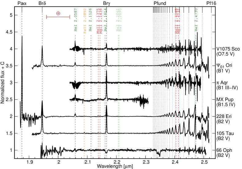
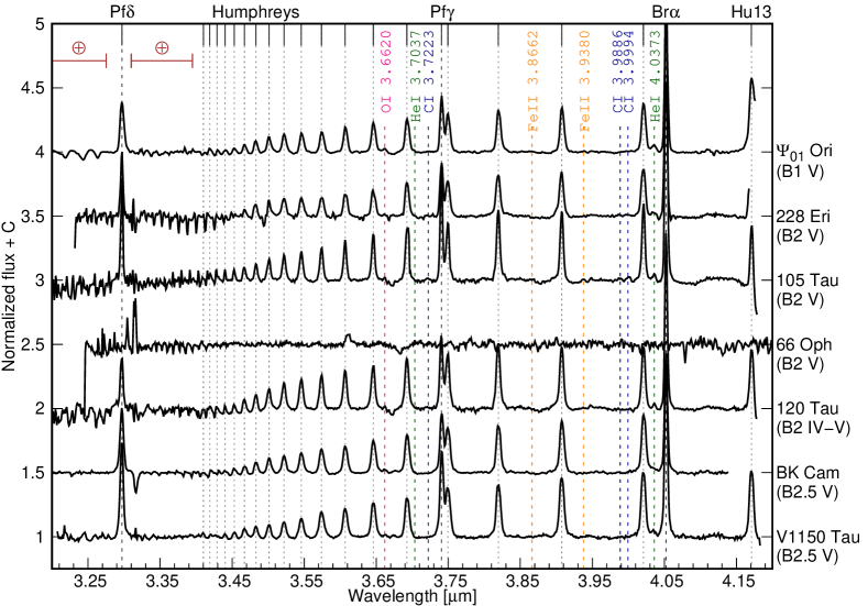
Figure 2: K- (upper panel) and L-band (lower panel) spectra of Be stars. Spectra are normalised and shifted vertically to ease comparison.

3.1 Hydrogen recombination lines

Our spectra cover a wide spectral range, where we have identified the following recombination hydrogen (H) lines: Pa$\alpha$ and Pa$\beta$; Br$\alpha$, and Br$\gamma$ up to the end of the series; Pf$\gamma$, Pf$\delta$, and Pf16 up to the end of the series; and Hu13 up to the end of the series. The H lines present different types of profiles. Most of the stars show H lines in emission above the continuum level, with one peak (e.g. $\Psi_{01}$ Ori) or two peaks (e.g. 12 Vul in the K band). There are some cases where the emission is weak and does not completely fill the photospheric absorption. In these cases the emission could be overimposed on the photospheric absorption (e.g 12 Vul in the H-band), resembling a shell-type profile (e.g. 28 Tau in the Brackett series) or barely visible as a deformation in the photospheric absorption-line profile (e.g. HD 171623 in the Pa$\beta$ and Br$\gamma$ lines). Spectra with no evidence of H emission lines are also observed (e.g. 66 Oph).

Tables 5 and 8 to 26 list the obtained line parameters for each object (except for 66 Oph and HD 171623, which present no evidence of H emission lines): EW, fluxes (Fl), full widths at half maximum (FWHM) and the peak separation of double-peaked line profiles ($\Delta\mathrm{V}$). The last two values are given in units of velocity. To obtain these parameters we performed Gaussian fittings to the emission components using IRAF tasks. The uncertainties for the measurements are around 10% for EW and Fl, 75 km s^-1 for FWHM, and 25 km s^-1 for $\Delta\mathrm{V}$. In this paper, we employ the convention that positive EW indicate emission features and negative EW indicate absorption features.

EWs and Fl for the H lines are corrected for photospheric absorption. For this purpose, we generated synthetic spectra with the synspec program (Hubeny, 1988; Hubeny & Lanz, 1995, 2011, 2017) using Kurucz (1979)’s atmosphere models as input. We used models with solar abundances, a microturbulence velocity of 2 km s^-1, and T_eff and $\log g$ in the ranges of $10\,000-39\,000$ K and $2.5-5$ dex, respectively. Steps for T_eff and $\log g$ were $1\,000$ K and $0.5$ dex, respectively. Table 4 summarises the selected $\log g$ range for each T_eff interval. Then, we measured the theoretical EWs of the H lines.

Table 4: Selected $\log g$ range for each T_eff interval.

Teff interval	$\log g$ range
[kK]	(dex)
10 - 11	2.0 - 5.0
12 - 19	2.5 - 5.0
20 - 26	3.0 - 5.0
27 - 31	3.5 - 5.0
32 - 39	4.0 - 5.0

We checked if the theoretical EWs are in good agreement with those previously reported for B stars. For the Pa$\beta$ lines we made a fitting of the T_eff versus EW behaviour using the values reported by Wallace et al. (2000) (Fig. 3 a), and compared it with the EW from the synthetic spectra (Fig. 3 b). The fitting was done using an implementation of the non-linear least-squares (NLLS) provided by GNUPLOT. In a similar way, Fig. 3 c presents the reported values of the EW of Br11 line from Meyer et al. (1998) for OB stars with luminosity classes V-III, and the comparison is in Fig. 3 d. Using a bigger sample from the APOGEE-2 DR14 catalogue (Abolfathi et al., 2018), Ramírez-Preciado et al. (2020) found a linear relationship between the sum of the EWs of the Br11 and Br13 lines and T_eff. This relationship, which is shown by a solid line in Fig. 3 e, falls in the upper limit of the theoretical EW values for stars with T_eff in the $10\,000-20\,000$ K range.

In the case of the Br$\gamma$ line, we used a fitting obtained from the measurements given by Hanson et al. (1996) (Figs. 3 f and g). Figures 3 h, i and j present the comparison of the EWs from the synthetic spectra with the fittings given by Lenorzer et al. (2002b). These fittings that give the relationship between the spectral type and the EW of some Brackett and Pfund lines were obtained empirically from a sample of 15 B-type dwarf to giant stars.

In general, we observe that the EWs obtained from the synthetic spectra are in good agreement with the values previously reported, especially in the T_eff and $\log g$ ranges typically observed in Be stars ($20\,000-30\,000$ K, $3.5-4.5$ dex, e.g. Cochetti et al., 2020). Then, we used the theoretical EWs to correct the observed H lines in our sample.

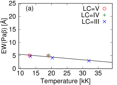
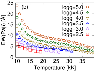
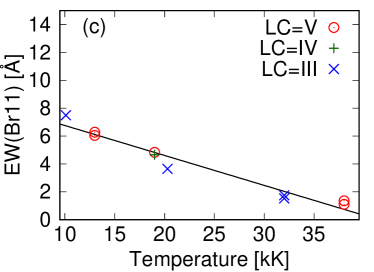
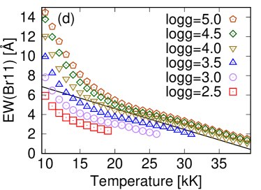
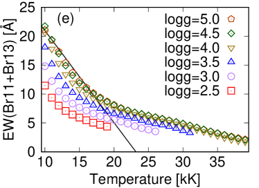
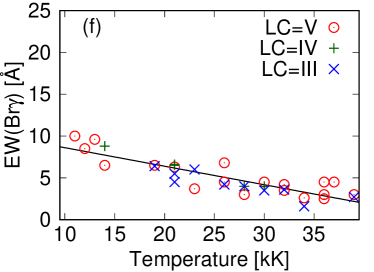
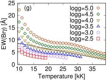
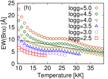
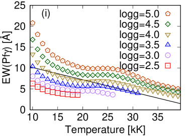
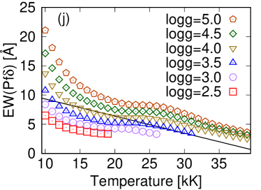
Figure 3: Comparison between EW obtained through synspec’s spectra and values/fits from the literature (see Sec. 3.1 for details).

Table 5: V1075 Sco - EW, Fl, and FWHM of the hydrogen lines.

Band/line	EW	Fl	FWHM
J band
Pa$\beta$	4.44	535.85	197
H band
Br10	3.79	157.54	313
Br11	3.07	144.84	438
Br12	2.31	115.05	529
Br13	em
Br14	1.81	104.26	502
Br15	1.97	116.7	478
Br16	1.7	103.57	509
Br17	1.7	104.69	540
Br18	1.33	83.74	521
Br19	1.2	77.31	587
K band
Br$\gamma$	6.2	121.38	244

3.2 Group classification

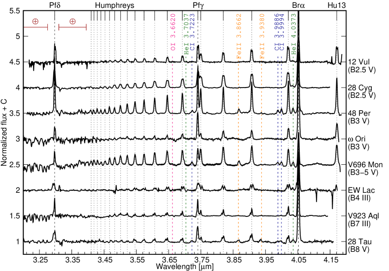
Figure 12: L-band spectra of Be stars. Spectra are normalised and shifted vertically to ease comparison.

Mennickent et al. (2009) proposed a criterion to classify the Be stars into three groups, based on the relative intensity of the hydrogen emission lines observed in the L band. Group I encompasses stars with Br$\alpha$ and Pf$\gamma$ lines with similar intensities to Humphreys lines. Stars with Br$\alpha$ and Pf$\gamma$ lines more intense than Humphreys lines belong to group II, while group III comprises stars with no emission lines. Following this criterion, we classified the stars of our sample with L-band observations (see Figs. 2 and 12) in the groups of Table 6.

Table 6: Group classification of our star sample according to Mennickent’s criterion.

Group I	Group II	Group III
BK Cam	$\Psi_{01}$ Ori∗	66 Oph
12 Vul	228 Eri∗
28 Cyg	105 Tau
V696 Mon	120 Tau∗
	V1150 Tau∗
	48 Per
	$\omega$ Ori
	EW Lac
	V923 Aql
	28 Tau
∗ Reclassified to group I (see Sec.4.1).

3.3 EW(Br$\alpha$)/EW(Br$\gamma$) ratio

According to the star sample analysed by Granada et al. (2010), group I objects present Br$\alpha$ and Br$\gamma$ lines with similar EW values up to EW(Br$\alpha$)$\simeq$3 EW(Br$\gamma$), while for stars in group II, the EW(Br$\alpha$) is much larger (more than five times) than the EW(Br$\gamma$). This behaviour is characteristic of the optically thick models, which predict a strong depression in the emission of Br$\alpha$ (Lynch et al., 2000).

In Fig. 4 we plot EW(Br$\alpha$) versus EW(Br$\gamma$) for the programme’s stars. Each star is represented with a different symbol. The empirical limits EW(Br$\alpha$)=3 EW(Br$\gamma$) and EW(Br$\alpha$)=5 EW(Br$\gamma$) are plotted in continuous and dashed lines, respectively, as a reference. Group I stars, which follow the same trend as the sample of Granada et al. (2010), are plotted in red. Group II stars are plotted in blue or green symbols according to the following criterion: those which follow the trend from Granada et al. (2010) EW(Br$\alpha$)$\gtrsim$5 EW(Br$\gamma$) are plotted in blue, and those with the EW(Br$\alpha$)/EW(Br$\gamma$) ratio similar to group I stars are plotted in green. We identify the green-symbol stars as group I-II. It is worth mentioning that 28 Cyg presents an EW(Br$\alpha$)/EW(Br$\gamma$) ratio a little higher than expected for a group I object.

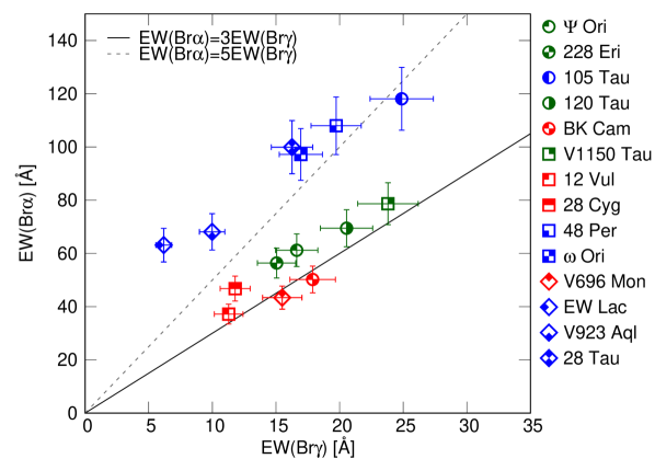
Figure 4: EW(Br$\alpha$) versus EW(Br$\gamma$). Red symbols are for group I stars, group II stars are plotted in blue, and green symbols are for the intermediate group I-II. The relations EW(Br$\alpha$)=3 EW(Br$\gamma$) and EW(Br$\alpha$)=5 EW(Br$\gamma$) are plotted in continuous and dashed lines, respectively.

3.4 Location in the Lenorzer diagram and other flux-ratio diagrams

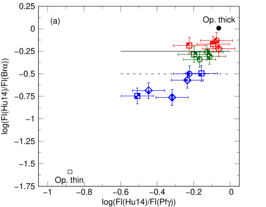
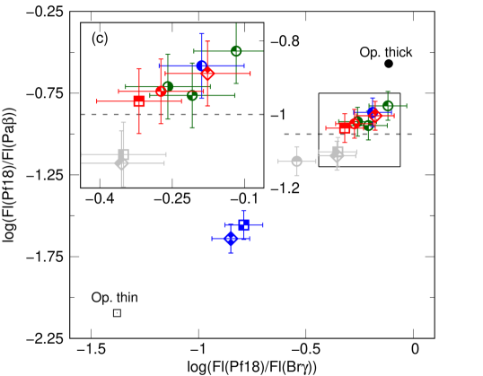
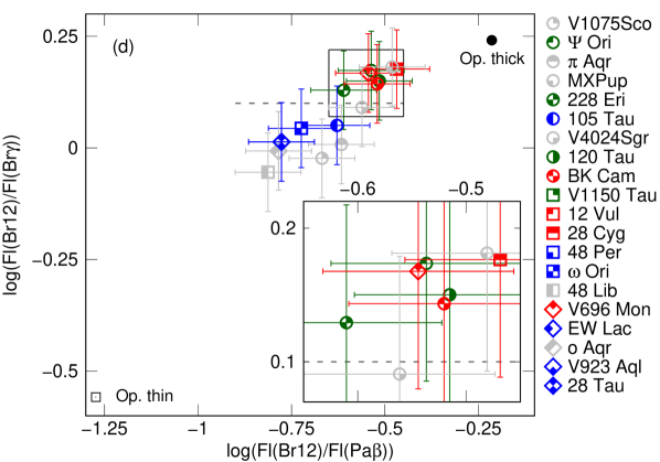
Figure 5: Flux-ratio diagrams based on the following lines: (a) Hu14 - Pf$\gamma$ - Br$\alpha$ (Lenorzer’s); (b) Br$\alpha$ - Pf$\gamma$ - Br$\gamma$ (Granada’s - Persson & McGregor’s); (c) Pf18 - Br$\gamma$ - Pa$\beta$; (d) Br12 - Pa$\beta$ - Br$\gamma$. The symbols for each star are the same as in Fig. 4, but the colour represents the group the star belongs to: red symbols represent group I stars, blue symbols group II stars, and green symbols the transition group I-II. The grey symbols are for those stars without an L-band spectrum and no group classification. Zoomed-in views of the region where symbols overlap are plotted in panels (c) and (d).

For a dense gas, lines are optically thick and their line strengths only depend on the emitting surface. On the contrary, for low gas densities, the lines are optically thin and can be represented by Menzel’s case B recombination (Baker & Menzel, 1938). Lenorzer et al. (2002a) made a diagram of the flux ratios Hu14/Br$\alpha$ versus Hu14/Pf$\gamma$ and plotted the location of different objects, together with the optically thick and optically thin limits. On this diagram, LBVs, Be, and B[e] stars are located in different loci along the diagonal between the optically thick and optically thin cases: LBVs are located in the lower part, close to the optically thin limit at (log(Fl(Hu14)/Fl(Pf$\gamma$)), log(Fl(Hu14)/Fl(Br$\alpha$))) $\simeq$ (-0.9,-1.6), Be stars are close to the optically thick case at (log(Fl(Hu14)/Fl(Pf$\gamma$)), log(Fl(Hu14)/Fl(Br$\alpha$))) $\simeq$ (0,0) in the upper part, while B[e] stars are in the central part. Moreover, Mennickent et al. (2009) located group I and II stars in a Lenorzer diagram and found that the group I stars are located in the top right part of the Lenorzer diagram, pointing out a compact and dense disc structure, while group II stars are more spread out and located in regions of moderate-to-small-line optical depths. Thereby, the location of the objects in the diagram gives us information about the density of the emitting gas.

Figure 5 a shows the Lenorzer diagram for those programme stars observed in the L band. The colour of the symbols in this figure is the same as in Fig 4. Stars of group I (BK Cam, 12 Vul, 28 Cyg, and V696 Mon) are located in the region log(Fl(Hu14)/Fl(Br$\alpha$)) $\geq$ -0.25 (limit marked with a solid black line), value that is close to the limit of -0.2 adopted by Mennickent et al. (2009) for stars in this group. For stars with log(Fl(Hu14)/Fl(Br$\alpha$)) below this value, classified as belonging to group II according to the intensity of Humphreys lines, we can distinguish between the ones that present EW(Br$\alpha$)/EW(Br$\gamma$) in the range expected for group II stars, and those with values nearer to the ones expected for stars of group I. Stars with EW(Br$\alpha$)/EW(Br$\gamma$) ratios in the expected range for group II stars (105 Tau, 48 Per, $\omega$ Ori, EW Lac, V923 Aql, and 28 Tau) are below the limit log(Fl(Hu14)/Fl(Br$\alpha$)) = -0.5 (dashed blue line). The others, which are those that present EW(Br$\alpha$)/EW(Br$\gamma$) ratios similar to those expected for group I ($\Psi_{01}$ Ori, 228 Eri, 120 Tau, and V1150 Tau), are located in the intermediate region -0.5 $\leq$ log(Fl(Hu14)/Fl(Br$\alpha$)) $\leq$ -0.25.

Granada et al. (2010) made a diagram similar to that of Persson & McGregor (1985) based on the Br$\alpha$, Pf$\gamma$, and Br$\gamma$ lines. They reported that these lines are also useful for distinguishing between compact thick or extended thin envelopes. Figure 5 b presents this diagram for our star sample, where stars of group I and I-II are located in the left part, while those of group II are located in the right part.

As observations in the L band are more difficult to obtain and both previously shown diagrams use lines from this band, we consider it useful to make a new diagram only based on lines from J, H, and K bands. With this aim, we made the diagrams shown in Figs. 5 c and d, which use the Pf18 - Br$\gamma$ - Pa$\beta$ and Br12 - Pa$\beta$ - Br$\gamma$ lines, respectively. The stars plotted in grey are those without an L-band spectrum and, therefore, without group classification and not plotted in Figs. 5 a and b.

The distributions obtained for the diagrams based on Pf18 - Br$\gamma$ - Pa$\beta$ and Br12 - Pa$\beta$ - Br$\gamma$ lines are similar to the one observed in the Lenorzer diagram. The group II stars are close to the optically thin limit in the lower part of the diagram at (log(Fl(Pf18)/Fl(Br$\gamma$)), log(Fl(Pf18)/Fl(Pa$\beta$))) $\simeq$ (-1.4,-2.1) and (log(Fl(Br12)/Fl(Pa$\beta$)), log(Fl(Br12)/Fl(Br$\gamma$))) $\simeq$ (-1.25,-0.6), while the group I stars are in the opposite corner, close to the optically thick case located at (log(Fl(Pf18)/Fl(Br$\gamma$)), log(Fl(Pf18)/Fl(Pa$\beta$))) $\simeq$ (-0.25,-0.6) and (log(Fl(Br12)/Fl(Pa$\beta$)), log(Fl(Br12)/Fl(Br$\gamma$))) $\simeq$ (-0.2,-0.25). The location of stars in group I-II is similar to that of stars in group I, and there is one star (105 Tau) classified as group II that falls in the upper region of the Pf18 - Br$\gamma$ - Pa$\beta$ diagram. It is worth mentioning that the position of 105 Tau in the Lenorzer diagram is over the line that divides the group II and I-II regions, so its location in Fig. 5 c suggests that it is likely an object belonging to group I-II. This intermediate classification may also indicate that these objects are in a transition stage between groups.

For the stars without group classification, there are three ($\pi$ Aqr, 48 Lib and $o$ Aqr) that are in the middle of the gap that separates the groups in Fig. 5 c and are located in a region compatible with group II in Fig. 5 d. V1075 Sco is located in the same region in Fig. 5 d. Thus, these four stars are likely part of group II.

Regarding the other two stars, in Fig. 5 d MX Pup is in a region compatible with group I stars, while V4024 Sgr falls in an intermediate locus. Based on that, MX Pup likely belongs to group I, and we can not assign a group for V4024 Sgr.

3.5 Helium and metallic lines

We identify lines from He i, C i, N i, O i, Na i, Mg i, Mg ii, Si i, Fe i, and Fe ii. In Tables 27 to 29, we present the EWs of the identified lines. As we mentioned before, positive EW indicate emission features, while negative EW indicate absorption features.

He i lines are present in 18 stars of our sample, generally in absorption, with the exception of the He I line at $\lambda\,2.0587\,\mu$m which is in emission. The Fe i and Fe ii lines are observed in emission in 16 and in 13 stars observed in the H band, respectively. In some of the stars that present Fe ii lines in emission in the H band, Fe ii lines are also observed in emission in the K and L bands. For the 19 objects observed in the J band, 15 stars present emission lines of O i, and 14 stars present C i in emission. Both elements also appear in the H- and L bands. Mg ii doublet $\lambda\lambda 2.1375-2.1438\,\mu$m is observed in 11 stars of the sample, while the other doublet in $\lambda\lambda 2.4038-2.4131\,\mu$m is more difficult to distinguish, because it is blended with H lines. Mg ii is also observed in the H band. In the H band, only five objects present N i emission at $\lambda\,1.5586\,\mu$m, while four present emission from Si i $\lambda\,1.5964\,\mu$m and $\lambda\,1.6064\,\mu$m. Two objects show Na i $\lambda\,2.2062\,\mu$m and $\lambda\,2.2090\,\mu$m in emission in the K band.

4 Discussion

4.1 An improved criterion to classify Be stars according to the disc opacity

Mennickent et al. (2009)’s criterion provides an easy way to separate stars in groups I and II through a qualitative description of the L-band spectrum of the Be stars, and thus to obtain information about the density of the emitting gas. However, in some cases where the Humphreys lines are quite intense, but not as intense as the Br$\alpha$ and Pf$\gamma$ lines, the classification may be ambiguous. In fact, we see that some stars classified as group II objects based on this criterion, actually have EWs and line-flux ratios similar to the ones of group I stars. Thus, we propose that the stars in our group I-II are indeed part of group I.

Assuming that stars in group I-II are actually part of group I, we can then quantitatively define different criteria that separate stars between groups I and II. These criteria, with limits represented by a dashed grey line in each panel of Fig. 5, are shown in Table 7. The criteria were empirically defined based on how the stars of each group gather in the different diagrams, separating group I objects from most group II objects. In Fig. 5 c, the unclassified objects laid in the gap between the group I and group II regions. Therefore, we used the information provided by Fig. 5 d, where the same unclassified objects are in positions compatible with group II membership. In Fig. 5 d, the limit could be a little displaced, because it is the only diagram where we can plot the unclassified object that is in the gap (V4024 Sgr).

With these new criteria, we can classify five of the seven stars without L-band observations. MX Pup is member of group I, while V1075 Sco, $\pi$ Aqr, 48 Lib, and $o$ Aqr are members of group II. We can also classify HD 171623 as a member of group III due to the absence of notorious emission. V4024 Sgr remains without classification because of its intermediate location in the Br12 - Pa$\beta$ - Br$\gamma$ area.

The final group classification for our sample is the following. Group I includes $\psi_{01}$ Ori, MX Pup, 228 Eri, 120 Tau, BK Cam, V1150 Tau, 12 Vul, 28 Cyg, and V696 Mon; Group II includes V1075 Sco, $\pi$ Aqr, 105 Tau, 48 Per, $\omega$ Ori, 48 Lib, EW Lac, $o$ Aqr, V923 Aql, and 28 Tau; Group III includes 66 Oph and HD 171623. V4024 Sgr remains unclassified.

It is worth highlighting that the nine stars that belong to group I have T${}_{\mathrm{eff}}\,\geq\,18000$, while seven of the ten stars in group II have T${}_{\mathrm{eff}}\,\leq\,18000$. The three stars in group II with T${}_{\mathrm{eff}}\,\geq\,18000$ are 105 Tau, for which we mentioned its limit position in the Lenorzer’s diagram, $\pi$ Aqr and V1075 Sco. This agrees with the result achieved by Sabogal et al. (2017), who mentioned that late Be stars present more tenuous and optically thin discs than early-type Be stars, but some early-type stars could present optically thin discs when they lose their discs.

Table 7: Quantitative criteria to classify stars in groups I and II, according to limits set on Fig. 5.

Ratio	Group I	Group II
log(Fl(Hu14)/Fl(Br$\alpha$))	$\gtrsim-0.5$	$\lesssim-0.5$
2.5$\cdot$log(Fl(Br$\alpha$)/Fl(Pf$\gamma$))	$\lesssim 0.55$	$\gtrsim 0.55$
log(Fl(Pf18)/Fl(Pa$\beta$))	$\gtrsim-1$	$\lesssim-1$
log(Fl(Br12)/Fl(Br$\gamma$))	$\gtrsim 0.1$	$\lesssim 0.1$

4.2 Behaviour of the He and metallic lines

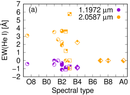
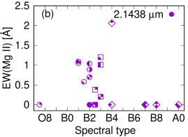
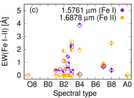
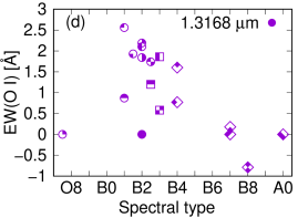
Figure 6: EW versus ST for representative lines of He i, Mg ii, Fe i, Fe ii and O i. The uncertainties for the EWs are around 10% of the values.

Figure 6 shows the EWs of representative lines from different elements versus the spectral type of the star. The symbols are the same as in Fig. 4, but different colours represent different lines of the same element, as is indicated in each panel.

In Fig. 6 a, we plot the EW values from the He i $\lambda\,2.0587\,\mu$m line in emission and the He i $\lambda\,1.1972\,\mu$m line in absorption. The He i is observed only in early B-type stars, with EW Lac (ST B4) and V696 Mon (ST B3-5) being the stars with the latest spectral type that present this element. This is in good agreement with previous results by Hanson et al. (1996), Clark & Steele (2000) and Lenorzer et al. (2002b).

The Mg ii $\lambda\,2.1438\,\mu$m line is only observed in the same spectral types as He lines (see Fig. 6 b). This agrees with the results by Clark & Steele (2000), who said that Mg II lines are likely excited via Ly$\beta$ fluorescence (Bowen, 1947) and are observed in stars with spectral types earlier than B4.

Regarding Fe i $\lambda\,1.5761\,\mu$m and Fe ii $\lambda\,1.6878\,\mu$m lines (Fig. 6 c), it seems that the emission is maximum for spectral types B2-B4. Through the comparison between the EWs of Fe ii, Mg ii and Br$\gamma$, Clark & Steele (2000) proposed that neither Fe ii nor Mg ii lines are seen in emission when EW(Br$\gamma$)$<8\,\AA$. We only have one object with EW(Br$\gamma$)$<8\,\AA$ (EW Lac), which does not present Fe ii or Mg ii emission in the K band.

Lenorzer et al. (2002b) reported that O i emission lines in the L band are observed in Be stars earlier than B3. However, in the K band we observe O i $\lambda\,1.3168\,\mu$m emission lines in stars with spectral types up to B7. It is worth mentioning that, as is shown in Fig. 6 d, the EW of O i emission lines becomes smaller for later spectral-type objects. This relation could be useful to estimate the ST of the star. In all the cases, EW(1.3168$\,\mu$m)/EW(1.129$\,\mu$m)¡1, as is expected if the Ly$\beta$ fluorescence process has a significant role in the excitation of the O i lines.

For the C i $\lambda\,1.1756\,\mu$m line, the existence of a correlation is not clear. Clark & Steele (2000) mentioned that the presence of Na i emission features suggests that a region of the circumstellar envelope should be shielded from direct stellar radiation, due to the low ionisation energy. This could be the case for 48 Per and V696 Mon, which are the two objects of our sample that present emission in Na i lines in the K band.

4.3 Correlation with $V\,\sin\,i$

To discuss if the main mechanism of broadening is rotational, we analyse the correlation between the FWHM and $\Delta\mathrm{V}$ parameters versus $V\,\sin\,i$. A strong correlation between the FWHM and $V\,\sin\,i$ was found by Hanuschik (1989) for optical lines and Granada et al. (2010) for IR lines.

The determination of the FWHM and $\Delta\mathrm{V}$ depends on the spectral resolution; therefore, to analyse their correlation with $V\,\sin\,i$ we selected GNIRS spectra. These spectra have the same resolution, and the sample is bigger than that observed with FIRE.

In Fig. 7, we plot the FWHM values of the Br10, Br$\delta$, Hu14, and Br$\alpha$ lines versus $V\,\sin\,i$. In each panel, a linear fitting and the 95% confidence interval are superimposed with a red line and grey area. To quantify the statistical relationship between the FWHM and $V\,\sin\,i$, we calculated the Pearson correlation coefficient for the distributions. For Br10, Br$\delta$, and Hu14 lines (Figs. 7 a, b, and c) we found a strong correlation with Pearson’s coefficients of 0.65, 0.67, and 0.60, respectively. Contrary to Granada et al. (2010), we found no correlation between the FWHM versus $V\,\sin\,i$ for the lines Pf$\gamma$ and Br$\alpha$ (see Fig. 7 d), nor for Br$\gamma$, Pa $\alpha$, Pa$\beta$, or Pf$\delta$ lines.

Figure 8 presents the peak separation versus $V\,\sin\,i$ for the same lines that the FWHM correlates with $V\,\sin\,i$ (Br10, Br$\delta$ and Hu14). It is seen that the $\Delta\mathrm{V}$ values on the Br10 line follow the relationship $\Delta\mathrm{V}=V\,\sin\,i$, which is plotted via a in dashed blue line. For the Hu14 line, the correlation is weaker, and there is no correlation for the Br$\delta$ line.

It is worth mentioning that those FWHMs and $\Delta\mathrm{V}$ that better correlate to $V\,\sin\,i$ correspond to higher-order Humphreys and Brackett lines, which form in inner parts of the disc compared the low-order lines (Hony et al., 2000; Mennickent et al., 2009), which form in outer parts. So, these lines might be useful when estimating the $V\,\sin\,i$ of the stars.

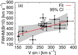
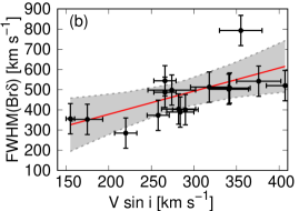
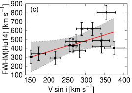
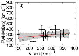
Figure 7: FWHMs of Br10 (a), Br$\delta$ (b), Hu14 (c), and Br$\alpha$ (d) lines versus $V\,\sin\,i$. Linear fits (red line) and 95% confidence intervals (grey area) are superimposed in each panel.

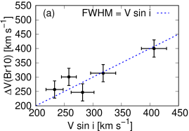
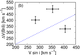
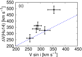
Figure 8: Peak separation of the Br10 (a), Br$\delta$ (b) and Hu14 (c) lines versus $V\,\sin\,i$. The linear relation $\Delta\mathrm{V}=V\,\sin\,i$ is represented by a dashed blue line.

5 Conclusions

The IR spectra of Be stars are excellent sources of information on the physical and dynamical structure of different regions inside the disc. Their analysis contributes to a better understanding of the possible mechanism involved in the development and evolution of the disc. However, a great number of NIR spectra and a wide spectral range coverage are required to attain a more complete overview of the Be phenomenon.

With this aim, we present an atlas of quasi simultaneous J-, H-, K-, and L-band observations of a sample of 22 Be stars obtained with the GNIRS and FIRE spectrographs. We identify several lines of the Paschen, Brackett, Pfund and Humphreys series of hydrogen. Lines of He i, C i, N i, O i, Na i, Mg i, Mg ii, Si i, Fe i, and Fe ii are also identified.

He i lines are observed in early B-type stars. In the same spectral types, the Mg ii and O i lines are observed in emission. Moreover, we report that the intensity of the O i $\lambda\,1.3168\,\mu$m emission line decreases towards the later spectral types. This reveals the importance of the Ly$\beta$ fluorescence process on Mg ii and O i transitions.

We also find a correlation between the FWHM of the Br10, Br$\delta$, and Hu14 lines with $V\,\sin\,i$. This indicates that the broadening mechanism is mainly rotational. In addition, the peak separation of Br10 line correlates strongly with $V\,\sin\,i$, while the correlation is weaker for the Hu14 line. We thus propose that these lines are useful when estimating the projected rotational velocity of Be stars.

Through the analysis of different hydrogen line-flux ratio diagrams, and taking into account the different value ranges from the EW(Br$\alpha$)/EW(Br$\gamma$) ratio, we propose new criteria to classify the Be stars into Mennickent’s groups. These new criteria also allow us to unify the classification that comes from previous works, which are the definition of the groups given by Mennickent et al. (2009) and the location of the different groups on Lenorzer’s diagram reported by Granada et al. (2010). Moreover, the new criteria involve lines not only in the L band, which are more difficult to obtain, but also in the J, H, and K bands. Using these criteria, we can identify some objects that present compact thick envelopes in our sample (group I stars: $\psi_{01}$ Ori, MX Pup, 228 Eri, 120 Tau, BK Cam, V1150 Tau, 12 Vul, 28 Cyg and V696 Mon), while in others the envelope is extended and optically thin (group II stars: V1075 Sco, $\pi$ Aqr, 105 Tau, 48 Per, $\omega$ Ori, 48 Lib, EW Lac, $o$ Aqr, V923 Aql and 28 Tau). The presence of an optically thin or thick disc seems to depend on $T_{\text{eff}}$, since group I stars have $T_{\text{eff}}\geq 18000$ while most group II stars have $T_{\text{eff}}\leq 18000$. We also find two objects that do not present an emitting disc at the observing time (66 Oph and HD 171623), and one star (V4024 Sgr) remains unclassified.

Paper II of this series will use the line parameters from this work to obtain a characterisation of the envelopes. It could be valuable to discuss the evolution of the envelopes through the analysis of the variability of their physical conditions and to identify some peculiar objects such as 12 Vul, which has presented a transitory ¹²CO emission (Cochetti et al., 2021). A better knowledge of the properties and evolution of the envelopes enable us to set constraints on the theoretical models of the stars with the Be phenomenon.

Appendix A Spectra of the star sample

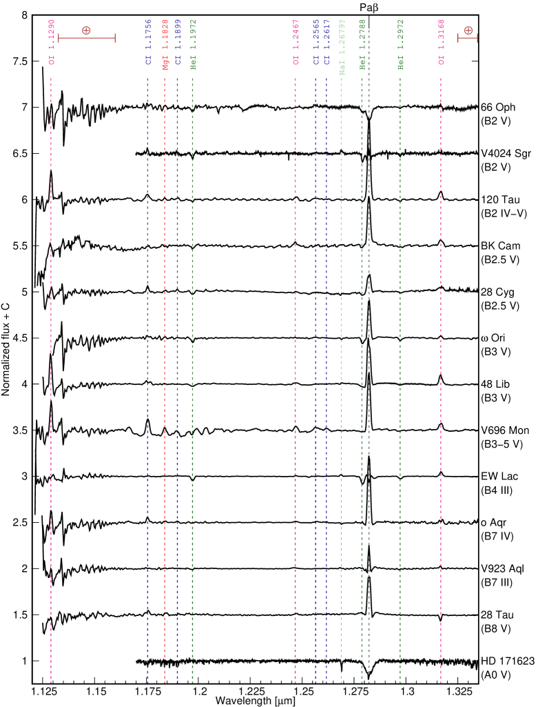
Figure 9: J-Band spectra of Be stars. Spectra are normalised and shifted vertically to ease comparison.

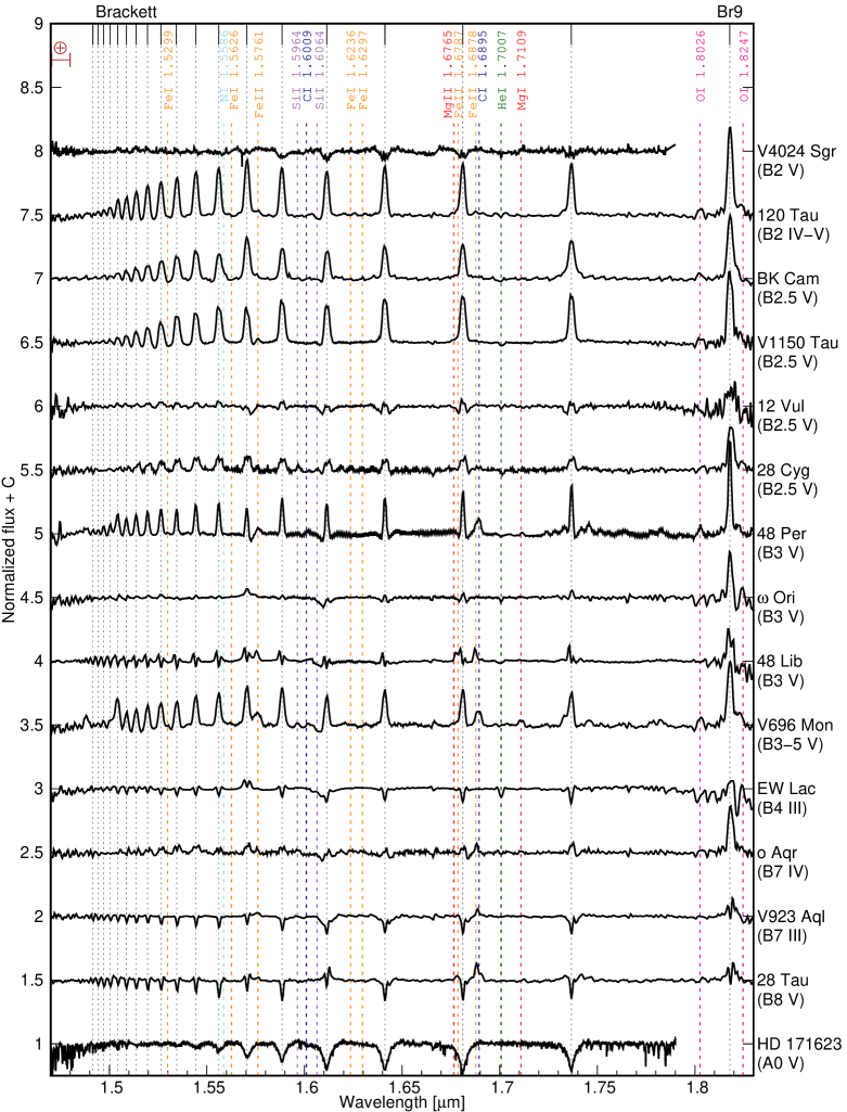
Figure 10: H-band spectra of Be stars. Spectra are normalised and shifted vertically to ease comparison.

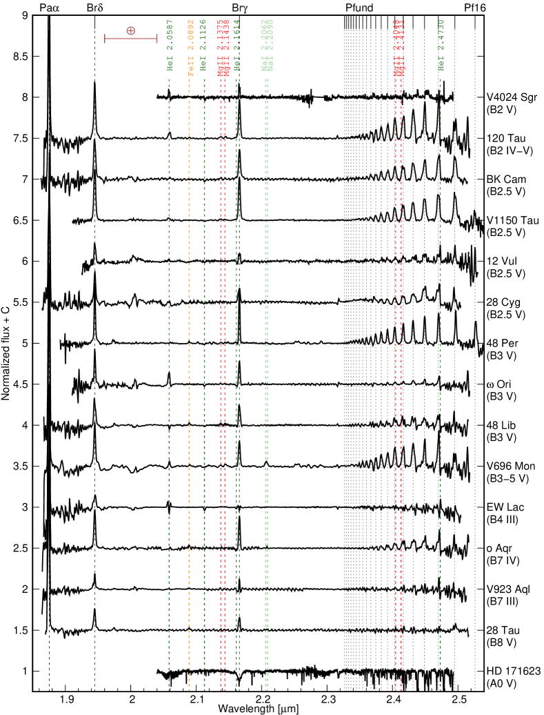
Figure 11: K-band spectra of Be stars. Spectra are normalised and shifted vertically to ease comparison.

Appendix B H-line parameters

The following tables show the line parameters of each H line for the star sample. The EW are in $\AA$, Fl are in units of 10^-13 erg cm^-2 s${}^{-1}\,\AA^{-1}$, and FWHM and $\Delta\mathrm{V}$ are in km s^-1.

Table 8: $\Psi$ Ori - EW, Fl, and FWHM of the hydrogen lines.

Band	Line	EW	Fl	FWHM
J-Band	Pa$\beta$	18.66	529.86	310
H-Band	Br9	27.89	312.63	472
	Br10	14.82	173	604
	Br11	13.21	162.21	524
	Br12	11.96	153.98	507
	Br13	10.41	139.14	475
	Br14	11.77	167.43	587
	Br15	12.87	193.56	608
	Br16	10.41	157.97	622
	Br17	9.38	146.95	608
	Br18	7.09	115.71	562
	Br19	6.56	111.16	511
	Br20	5.31	92.45	509
	Br21	3.68	66.3	477
	Br22	2.09	39.02	393
	Br23	1.65	31.41	341
	Br24	0.92	18.03	341
K-Band	Pf17	em
	Pf18	17.49	78.78	448
	Pf19	9.52	44.62	305
	Pf20	12.18	57.09	560
	Pf21	9.21	43.61	568
	Pf22	7.37	35.7	476
	Pf23	5.90	28.71	507
	Pf24	4.47	22.05	423
	Pf25	3.31	16.55	398
	Pf26	2.10	10.81	376
	Pf27	1.32	6.9	273
	Pf28	0.78	4.12	188
	Pf29	0.60	3.17	190
	Br$\gamma$	16.63	103.25	332
	Br$\delta$	27.16	234.27	544
L-Band	Hu13	em
	Br$\alpha$	61.20	109.37	272
	Hu14	27.10	49.81	424
	Hu15	28.62	55.61	510
	Hu16	27.22	57.98	547
	Hu17	23.33	53.96	540
	Pf$\gamma$	31.46	73.30	368
	Hu18	20.85	50.91	552
	Hu19	16.62	42.98	530
	Hu20	14.52	38.57	531
	Hu21	12.36	33.87	563
	Hu22	11.33	31.89	543
	Hu23	9.95	29.03	527
	Hu24	8.54	25.58	540
	Hu25	5.91	18.07	437
	Hu26	3.98	12.42	413
	Hu27	2.96	9.35	491
	Hu28	2.21	7.11	479
	Hu29	1.67	5.41	$\cdots$
	Pf$\delta$	19.69	73.90	222

Table 9: $\pi$ Aqr - EW, Fl, FWHM, and $\Delta V$ of the hydrogen lines.

Band	Line	EW	Fl	FWHM	$\Delta V$
J-Band	Pa$\beta$	10.12	41.82	357	212
H-Band	Br10	6.2	9.7	$\cdots$	257
	Br11	5.85	9.81	$\cdots$	247
	Br12	5.93	10.11	455	251
	Br13	4.2	7.47	393	272
	Br14	5.54	10.37	500	288
	Br15	4.93	9.64	473	268
	Br16	4.68	9.63	495	293
	Br17	4.88	10.39	514	287
	Br18	4.6	10.21	491	274
	Br19	4	9.16	490	281
	Br20	3.55	8.4	474	274
	Br21	3.96	9.52	483	275
	Br22	2.63	6.41	480	276
	Br23	2.25	5.62	492	269
K-Band	Pf17	8.19	4.67	$\cdots$	250
	Pf18	4.85	2.85	$\cdots$	268
	Pf19	6.73	3.99	$\cdots$	307
	Pf20	4.39	2.67	$\cdots$	278
	Pf21	6.44	3.94	$\cdots$	$\cdots$
	Pf22	4.37	2.76	$\cdots$	$\cdots$
	Pf23	3.69	2.37	$\cdots$	$\cdots$
	Pf24	3.51	2.29	$\cdots$	$\cdots$
	Pf25	3.19	2.11	$\cdots$	$\cdots$
	Pf26	2.16	1.45	$\cdots$	$\cdots$
	Pf27-28	em
	Br$\gamma$	10.51	9.93	359	211

Table 10: MX Pup - EW, Fl, FWHM, and $\Delta V$ of the hydrogen lines.

Band	Line	EW	Fl	FWHM	$\Delta V$
J-Band	Pa$\beta$	18.52	39.71	191	98
H-Band	Br10	15.93	12.55	290	116
	Br11	15.79	13.06	310	117
	Br12	14.53	13.13	310	112
	Br13	13.34	12.73	316	144
	Br14	13.72	13.52	339	137
	Br15	13.35	13.49	338	127
	Br16	12.12	12.86	335	106
	Br17	11.28	12.32	345	115
	Br18	9.99	11.19	340	101
	Br19	8.52	9.82	340	113
	Br20	7.21	8.51	336	114
	Br21	4.60	5.71	286	124
	Br22	4.49	5.55	308	111
	Br23	3.25	4.14	295	161
	Br24	2.30	2.99	266	133
	Br25	2.01	2.64	285	140
	Br26	1.63	2.15	286	134
	Br27	1.27	1.71	297	$\cdots$
	Br28-29	em
K-Band	Br$\gamma$	20.90	8.65	229	102

Table 11: 228 Eri - EW, Fl, and FWHM of the hydrogen lines.

Band	Line	EW	Fl	FWHM
J-Band	Pa$\beta$	15.97	343.01	301
H-Band	Br9	21.98	130.5	528
	Br10	11.17	85.2	467
	Br11	9.92	83.61	442
	Br12	9.35	84.11	459
	Br13	8.14	77.73	462
	Br14	8.78	88.57	559
	Br15	11.07	115.92	629
	Br16	7.08	76.1	564
	Br17	6.56	72.22	558
	Br18	5.70	64.08	576
	Br19	4.86	55.91	563
	Br20	4.27	50.18	529
	Br21	2.88	34.7	465
	Br22	1.80	22.24	434
	Br23	1.27	16.07	392
	Br24-26	em
K-Band	Pf16-17	em
	Pf18	17.13	38.64	463
	Pf19	8.72	21.56	377
	Pf20	12.39	30.06	600
	Pf21	7.56	19.26	533
	Pf22	6.87	18.19	483
	Pf23	5.12	13.96	520
	Pf24	3.98	11.15	426
	Pf25	3.04	8.68	412
	Pf26	2.83	8.26	622
	Pf27	0.87	2.61	$\cdots$
	Pf28	1.10	3.28	$\cdots$
	Pf29	0.71	2.17	$\cdots$
	Pf30-31	em
	Br$\gamma$	15.05	62.45	321
	Br$\delta$	22.80	123.95	508
	Pa$\alpha$	63.88	338.67	279
L-Band	Hu13	em
	Br$\alpha$	56.39	33.13	255
	Hu14	26.36	16.36	422
	Hu15	29.71	18.91	554
	Hu16	22.87	16.09	504
	Hu17	21.03	15.27	523
	Pf$\gamma$	29.11	21.21	362
	Hu18	18.55	14.05	489
	Hu19	16.04	12.44	586
	Hu20	12.99	10.36	550
	Hu21	12.49	10.05	613
	Hu22	10.31	8.46	552
	Hu23	8.60	7.22	515
	Hu24	5.21	4.40	320
	Hu25	6.31	5.32	434
	Hu26	2.52	2.17	324
	Pf$\delta$	25.98	28.90	295

Table 12: 105 Tau - EW, Fl, and FWHM of the hydrogen lines.

Band	Line	EW	Fl	FWHM
J-Band	Pa$\beta$	27.52	598.77	217
H-Band	Br9	27.72	235.55	343
	Br10	16.04	146.26	350
	Br11	14.9	143.85	343
	Br12	13.93	140.94	346
	Br13	12.2	128.82	343
	Br14	12.25	139.11	384
	Br15	14.18	166.5	463
	Br16	10.62	127.77	425
	Br17	9.5	117.73	420
	Br18	7.5	96.06	399
	Br19	7.41	97.26	403
	Br20	6.29	84.31	399
	Br21	4.6	63.6	370
	Br22	3.48	49.32	352
	Br23	2.97	42.99	318
	Br24	1.57	23.46	$\cdots$
	Br25	0.99	15.15	$\cdots$
K-Band	Pf17	em
	Pf18	25.18	81.19	353
	Pf19	13.83	48.22	275
	Pf20	16.42	57.41	533
	Pf21	12.8	45.55	491
	Pf22	9.23	33.88	418
	Pf23	7.11	26.51	420
	Pf24	5.72	21.6	356
	Pf25	4.51	17.29	360
	Pf26	3.69	14.48	426
	Pf27	2.21	8.83	$\cdots$
	Pf28	1.63	6.58	$\cdots$
	Pf29	1.02	4.19	$\cdots$
	Pf30	0.76	3.14	$\cdots$
	Br$\gamma$	24.88	125.46	259
	Br$\delta$	31.07	216.29	353
L-Band	Br$\alpha$	118.11	75.06	197
	Hu14	34.44	23.74	339
	Hu15	32.89	25.28	372
	Hu16	33.37	28.16	406
	Hu17	26.61	24.31	408
	Pf$\gamma$	43.10	39.68	265
	Hu18	18.85	18.53	347
	Hu19	17.78	18.13	357
	Hu20	16.44	17.14	384
	Hu21	15.62	16.69	444
	Hu22	13.46	14.96	459
	Hu23	11.11	12.71	439
	Hu24	8.96	10.5	425
	Hu25	6.53	7.76	368
	Hu26	5.50	6.65	396
	Hu27	3.36	4.12	$\cdots$
	Hu28	2.27	2.83	$\cdots$
	Pf$\delta$	33.28	49.99	263

Table 13: V4024 Sgr - EW, Fl, FWHM, and $\Delta V$ of the hydrogen lines.

Band	Line	EW	Fl	FWHM	$\Delta V$
J-Band	Pa$\beta$	6.19	1282.20	$\cdots$	187
H-Band	Br10	em
	Br11	4.59	367.65	$\cdots$
	Br12	4.22	352.06	$\cdots$
	Br13	3.40	320.73	$\cdots$
	Br14	2.76	276.09	$\cdots$
K-Band	Br$\gamma$	8.18	285.61	295	181

Table 14: 120 Tau - EW, Fl, and FWHM of the hydrogen lines.

Band	Line	EW	Fl	FWHM
J-Band	Pa$\beta$	20.46	1019.65	308
H-Band	Br9	25.75	359.46	448
	Br10	16.84	302.77	447
	Br11	14.64	300.85	415
	Br12	14.14	311.4	436
	Br13	13.19	304.5	453
	Br14	13.20	324.34	468
	Br15	13.41	345.52	475
	Br16	11.01	286.59	454
	Br17	10.07	267.08	456
	Br18	9.09	243.23	458
	Br19	8.45	230.96	475
	Br20	7.27	201.9	431
	Br21	5.75	162.68	411
	Br22	4.18	121	384
	Br23	3.08	91.63	329
	Br24	1.46	44.76	331
	Br25	0.72	22.39	246
	Br26	0.46	14.59	228
K-Band	Pf17	em
	Pf18	23.96	121.38	364
	Pf19	12.54	70.45	309
	Pf20	13.97	80.41	465
	Pf21	11.72	69.69	470
	Pf22	11.74	72.31	482
	Pf23	9.07	58.12	502
	Pf24	6.43	43.04	421
	Pf25	4.98	34.12	352
	Pf26	5.08	35.74	510
	Pf27	1.25	9.25	253
	Pf28	1.22	9.05	224
	Pf29	1.05	7.85	264
	Br$\gamma$	20.55	220.39	376
	Br$\delta$	29.53	405.48	487
	Pa$\alpha$	81.98	1072.18	338
L-Band	Hu13	em
	Br$\alpha$	69.47	50.08	263
	Hu14	35.66	27.62	435
	Hu15	35.76	30.49	476
	Hu16	35.41	33.47	479
	Hu17	29.53	30.06	485
	Pf$\gamma$	36.06	37.01	355
	Hu18	29.28	30.83	521
	Hu19	21.83	24.48	477
	Hu20	19.26	22.12	482
	Hu21	17.39	20.49	489
	Hu22	15.05	18.31	487
	Hu23	12.38	15.63	480
	Hu24	10.81	13.96	529
	Hu25	7.55	9.91	427
	Hu26	5.72	7.64	401
	Hu27	3.45	4.68	368
	Hu28	2.20	3.02	216
	Hu29	2.50	3.49	331
	Pf$\delta$	25.92	41.68	382

Table 15: BK Cam - EW, Fl, and FWHM of the hydrogen lines.

Band	Line	EW	Fl	FWHM
J-Band	Pa$\beta$	15.04	552.22	325
H-Band	Br9	25.4	269.77	586
	Br10	17.82	217.73	689
	Br11	12.78	172.52	473
	Br12	11.38	166.64	454
	Br13	10.36	158.14	474
	Br14	10.2	165.02	514
	Br15	12.41	210.03	564
	Br16	9.07	155.4	632
	Br17	7.86	141.84	539
	Br18	7.02	128.89	575
	Br19	5.65	106.08	542
	Br20	4.17	80.68	539
	Br21	3.03	59.79	491
	Br22	2.05	41.35	449
	Br23	1.18	24.46	456
	Br24-25	em
K-Band	Pf17	17.39	68.83	592
	Pf18	15.65	63.82	517
	Pf19	12.54	52.83	545
	Pf20	12.77	54.57	613
	Pf21	9.76	42.9	606
	Pf22	7.46	33.66	507
	Pf23	5.28	24.41	518
	Pf24	3.93	18.52	397
	Pf25	2.99	14.32	452
	Pf26	2.97	14.48	571
	Pf27	1.1	5.44	299
	Pf28	0.49	2.48	$\cdots$
	Pf29	0.71	3.59	$\cdots$
	Br$\gamma$	17.88	119.76	401
	Br$\delta$	24.03	221.82	502
	Pa$\alpha$	69.13	689.22	409
L-Band	Br$\alpha$	50.2	40.22	303
	Hu14	35.93	29.8	489
	Hu15	34.39	31	553
	Hu16	31.22	30.33	553
	Hu17	26.45	27.67	525
	Pf$\gamma$	33.67	35.39	405
	Hu18	22.48	24.24	527
	Hu19	18.17	20.42	530
	Hu20	15.62	17.98	554
	Hu21	14.71	17.32	584
	Hu22	10.96	13.35	558
	Hu23	8.66	10.84	510
	Hu24	8.39	10.69	561
	Hu25	5.95	7.72	500
	Hu26	4.33	5.69	514
	Hu27	3.38	4.51	517
	Pf$\delta$	28.09	45.81	343

Table 16: V1150 Tau - EW, Fl, and FWHM of the hydrogen lines.

Band	Line	EW	Fl	FWHM
H-Band	Br9	25.45	23.66	489
	Br10	17.94	19.06	497
	Br11	17.45	20.53	522
	Br12	15.88	20.32	521
	Br13	13.56	18.18	504
	Br14	14.08	19.66	557
	Br15	10.78	15.31	519
	Br16	10.61	15.71	558
	Br17	9.7	14.57	575
	Br18	8.69	13.48	570
	Br19	7.01	11.07	558
	Br20	5.32	8.64	528
	Br21	3.61	6.02	473
	Br22	2.22	3.8	437
	Br23	1.53	2.68	424
	Br24	0.84	1.5	418
	Br25	0.49	0.89	482
K-Band	Pf17	24.38	9.53	695
	Pf18	17.23	7.07	535
	Pf19	15.05	6.34	582
	Pf20	11.7	5.08	537
	Pf21	9.32	4.17	537
	Pf22	7.67	3.51	498
	Pf23	5.61	2.61	509
	Pf24	3.9	1.85	432
	Pf25	2.85	1.38	409
	Pf26	2.19	1.08	502
	Pf27	1.06	0.53	345
	Pf28	0.62	0.31	301
	Br$\gamma$	23.8	15.72	389
	Br$\delta$	29.56	25.97	498
L-Band	Hu13	51.98	5.1	557
	Br$\alpha$	78.68	8.32	304
	Hu14	39.76	4.32	478
	Hu15	40.75	4.69	561
	Hu16	36.86	4.52	607
	Hu17	35.19	4.65	659
	Pf$\gamma$	51	6.81	479
	Hu18	28.97	3.97	661
	Hu19	25.11	3.56	686
	Hu20	18.01	2.65	640
	Hu21	16.67	2.51	676
	Hu22	10.92	1.68	574
	Hu23	9.77	1.54	572
	Hu24	7.06	1.14	488
	Hu25	4.46	0.74	388
	Hu26	3.54	0.6	395
	Hu27	2.21	0.37	375
	Hu28	1.26	0.22	320
	Pf$\delta$	44.55	8.59	418

Table 17: 12 Vul - EW, Fl, FWHM, and $\Delta V$ of the hydrogen lines.

Band	Line	EW	Fl	FWHM	$\Delta V$
H-Band	Br9	em
	Br10	8.52	51.11	464	301
	Br11	7.88	53.63	417	276
	Br12	6.69	50.72	453	266
	Br13	4.96	40.44	413	277
	Br14	4.18	36.7	395	257
	Br15	3.05	26.73	435	264
	Br16	2.23	20.95	371	264
	Br17	1.82	17.45	574	270
	Br18	1.35	13.22	455	309
	Br19	1.5	15.02	553	$\cdots$
	Br20	1.19	12.14	607	$\cdots$
K-Band	Pf18	4.05	6.62	$\cdots$	$\cdots$
	Pf19	6.01	10.2	$\cdots$	$\cdots$
	Pf20	6.29	10.9	$\cdots$	$\cdots$
	Pf21	3.46	6.19	$\cdots$	$\cdots$
	Pf22	2.86	5.23	$\cdots$	$\cdots$
	Pf23	2.5	4.7	$\cdots$	$\cdots$
	Br$\gamma$	11.28	30.78	429	267
	Br$\delta$	13.31	54.4	373	$\cdots$
L-Band	Hu13	27.62	8.61	420	262
	Br$\alpha$	37.2	11.99	391	240
	Hu14	23.46	7.82	439	263
	Hu15	17.69	6.51	436	278
	Hu16	14.34	5.69	448	261
	Hu17	13.3	5.55	441	229
	Pf$\gamma$	31.45	13.1	450	264
	Hu18	8.8	3.97	457	276
	Hu19	6.67	3.14	434	266
	Hu20	4.64	2.28	433	231
	Hu21	4.19	2.12	451	244
	Hu22	3.96	2.05	482	264
	Hu23	3.37	1.79	493	244
	Hu24	2.5	1.36	458	247
	Hu25	1.91	1.06	457	224
	Hu26	2.1	1.18	577	310
	Pf$\delta$	24.36	16.71	414	257

Table 18: 28 Cyg - EW, Fl, FWHM, and $\Delta V$ of the hydrogen lines.

Band	Line	EW	Fl	FWHM	$\Delta V$
J-Band	Pa$\beta$	8.78	172.70	386	$\cdots$
H-Band	Br9	18.55	95.2	571	$\cdots$
	Br10	7.99	51.67	576	314
	Br11	7.04	53.51	506	345
	Br12	7.08	58.72	556	343
	Br13	5.87	52.36	540	368
	Br14	6.56	61.52	669	348
	Br15	6.18	60.45	624	374
	Br16	5.25	52.74	663	362
	Br17	5.02	51.29	686	359
	Br18	3.87	40.04	653	379
	Br19	3.1	32.27	610	344
	Br20	2.79	29.18	617	$\cdots$
	Br21	1.96	20.86	611	$\cdots$
	Br22-23	em
K-Band	Pf17	em
	Pf18	11.92	21.86	600	$\cdots$
	Pf19	9.6	18.77	666	350
	Pf20	7.5	14.43	751	395
	Pf21	5.25	10.13	591	481
	Pf22	3.94	7.74	545	357
	Pf23	2.97	5.99	534	303
	Pf24	2.32	4.86	611	$\cdots$
	Br$\gamma$	11.79	39.11	484	$\cdots$
	Br$\delta$	19.94	87.21	513	$\cdots$
	Pa$\alpha$	52.66	224.28	493	$\cdots$
L-Band	Br$\alpha$	46.79	20.88	393	$\cdots$
	Hu14	30.82	14.1	621	326
	Hu15	26.74	13.46	621	336
	Hu16	25.76	14	666	327
	Hu17	19.55	11.5	611	341
	Pf$\gamma$	29.47	17.51	537	165
	Hu18	16.45	10.15	636	327
	Hu19	13.06	8.45	612
	Hu20	11.53	7.75	671
	Hu21	8.76	6.1	608
	Hu22	7.13	5.13	584
	Hu23	6.42	4.75	621
	Hu24	6.95	5.28	652
	Hu25	5.75	4.47	642
	Hu26	2.37	1.88	529
	Hu27	3.13	2.53	632
	Hu28-29	em
	Pf$\delta$	30.6	30.14	546	237

Table 19: 48 Per - EW, Fl, and FWHM of the hydrogen lines.

Band	Line	EW	Fl	FWHM
H-Band	Br9	19.28	571.26	242
	Br10	11.76	369.51	188
	Br11	10.92	364.62	206
	Br12	9.92	349.66	216
	Br13	9.31	344.56	250
	Br14	8.25	339.4	246
	Br15	6.38	271.02	224
	Br16	6.23	278.35	248
	Br17	5.70	261.76	279
	Br18	4.01	188.7	220
	Br19	4.51	215.7	306
	Br20	4.13	200.08	310
	Br21	3.32	163.87	300
	Br22	2.50	125.7	288
	Br23	3.06	159.1	331
	Br24-27	em
K-Band	Pf16	em
	Pf17	12.91	121.67	265
	Pf18	12.16	119.86	288
	Pf19	11.29	112.26	310
	Pf20	9.38	95.37	328
	Pf21	7.35	75.98	317
	Pf22	6.94	72.56	359
	Pf23	5.43	57.81	311
	Pf24	3.64	39.94	285
	Pf25	3.71	40.8	312
	Pf26	3.19	35.11	341
	Pf27	2.14	24.12	254
	Pf28	1.48	16.95	216
	Pf29	1.06	12.34	209
	Pf30	1.12	13.14	306
	Pf31	0.52	6.24	$\cdots$
	Pf32	0.53	6.38	$\cdots$
	Pf33	0.28	3.35	$\cdots$
	Pf34	0.27	3.21	$\cdots$
	Pf35	0.13	1.52	$\cdots$
	Br$\gamma$	19.73	287.95	197
	Br$\delta$	23.39	504.61	285
L-Band	Hu13	39.43	78.99	286
	Br$\alpha$	107.97	227.92	170
	Hu14	34.86	72.82	292
	Hu15	31.41	71.15	304
	Hu16	29.05	69.09	337
	Hu17	24.36	63.10	337
	Pf$\gamma$	39.96	104.71	228
	Hu18	20.43	54.11	332
	Hu19	18.95	51.69	358
	Hu20	15.06	42.40	351
	Hu21	13.58	39.16	377
	Hu22	13.04	38.72	439
	Hu23	8.79	26.83	347
	Hu24	7.96	24.57	378
	Hu25	5.07	15.99	334
	Hu26	5.60	17.91	317
	Hu27	3.78	12.22	326
	Hu28	3.47	11.34	347
	Hu29	3.86	12.82	311
	Hu30	3.64	12.17	337
	Hu31	3.97	13.49	449
	Pf$\delta$	43.62	173.86	255

Table 20: $\omega$ Ori - EW, Fl, and FWHM of the hydrogen lines.

Band	Line	EW	Fl	FWHM
J-Band	Pa$\beta$	15.75	554.74	302
H-Band	Br9	19.28	210.59	389
	Br10	8.96	112.86	255
	Br11	8.44	114.40	314
	Br12	7.17	104.80	209
	Br13	6.21	95.13	362
	Br14	4.62	78.96	289
	Br15-20	em
K-Band	Pf18	4.18	15.4	279
	Pf19	2.42	9.26	257
	Pf20	2.49	9.69	495
	Pf21	1.14	4.51	342
	Pf22	1.24	5.01	415
	Pf23	0.99	4.03	289
	Br$\gamma$	16.95	94.73	312
	Br$\delta$	20.77	178.38	356
L-Band	Hu13	em
	Br$\alpha$	97.18	39.33	304
	Hu14	15.92	7.06	334
	Hu15	14.78	7.34	447
	Hu16	12.99	7.33	458
	Hu17	7.54	4.65	351
	Pf$\gamma$	36.96	22.78	342
	Hu18	4.83	3.23	314
	Hu19	4.10	2.86	336
	Hu20	3.81	2.72	455
	Hu21	2.73	2.02	376
	Hu22	2.48	1.9	414
	Hu23	1.85	1.48	316
	Hu24	1.31	1.08	457
	Hu25	1.61	1.32	313
	Hu26-27	em
	Pf$\delta$	19.90	20.33	327

Table 21: 48 Lib - EW, Fl, FWHM, and $\Delta V$ of the hydrogen lines.

Band	Line	EW	Fl	FWHM	$\Delta V$
J-Band	Pa$\beta$	16.46	599.27	373	233
H-Band	Br9	18.72	229.36	$\cdots$	378
	Br10	7.16	102.19	$\cdots$	400
	Br11	8.22	126.03	$\cdots$	356
	Br12	5.70	92.23	$\cdots$	434
	Br13	4.69	80.35	$\cdots$	423
	Br14	3.91	73.99	$\cdots$	488
	Br15	3.84	77.32	$\cdots$	478
	Br16	2.98	61.05	$\cdots$	519
	Br17	1.74	37.03	$\cdots$	498
	Br18	1.49	32.35	$\cdots$	519
	Br19	1.12	25.01	$\cdots$	508
	Br20	0.93	21.18	$\cdots$	540
K-Band	Pf18	11.41	46.61	$\cdots$	320
	Pf19	9.82	42.6	$\cdots$	262
	Pf20	9.18	40.54	$\cdots$	491
	Pf21	4.62	21.8	$\cdots$	426
	Pf22	3.78	18.4	$\cdots$	407
	Pf23	3.52	17.18	$\cdots$	484
	Pf24	2.45	12.3	$\cdots$	441
	Pf25	1.26	6.44	$\cdots$	$\cdots$
	Br$\gamma$	15.39	104.56	377	234
	Br$\delta$	18.63	194.6	520	329
	Pa$\alpha$	108.90	1201.24	374	$\cdots$

Table 22: V696 Mon - EW, Fl, and FWHM of the hydrogen lines.

Band	Line	EW	Fl	FWHM
J-Band	Pa$\beta$	16.83	721.09	321
H-Band	Br9	23.79	312.17	531
	Br10	13.51	214.48	542
	Br11	11.49	198.55	389
	Br12	11.18	206	424
	Br13	9.55	186.56	403
	Br14	10.89	229.88	465
	Br15	11.30	244.67	534
	Br16	7.47	167.11	442
	Br17	6.62	151.32	428
	Br18	5.78	133.76	417
	Br19	5.33	127.57	435
	Br20	5.21	125.52	421
	Br21	4.83	116.74	431
	Br22	3.06	76.99	363
K-Band	Pf17	em
	Pf18	17.93	93.21	336
	Pf19	9.78	53.47	285
	Pf20	14.49	77.67	506
	Pf21	10.68	60.41	472
	Pf22	8.57	51.28	417
	Pf23	7.39	45.14	457
	Pf24	6.16	38.72	408
	Pf25	5.51	34.58	351
	Pf26	5.09	32.88	471
	Pf27	1.90	12.82	228
	Pf28	1.88	12.75	241
	Pf29	1.42	9.65	232
	Br$\gamma$	15.49	140.01	353
	Br$\delta$	27.33	321.11	542
	Pa$\alpha$	66.46	878.84	373
L-Band	Hu13	28.73	30.68	409
	Br$\alpha$	43.39	50.46	308
	Hu14	24.58	30.33	402
	Hu15	25.17	32.36	436
	Hu16	25.42	34	475
	Hu17	21.45	30.46	436
	Pf$\gamma$	24.66	35.05	350
	Hu18	20.52	30.59	512
	Hu19	16.81	25.94	462
	Hu20	14.38	22.54	432
	Hu21	12.66	20.34	432
	Hu22	12.67	20.77	460
	Hu23	9.96	16.88	422
	Hu24	10.18	17.6	468
	Hu25	8.15	14.28	426
	Hu26	6.59	11.78	381
	Hu27	4.36	7.86	436
	Hu28	3.20	5.83	388
	Hu29	3.13	5.85	$\cdots$
	Hu30	5.27	9.84	$\cdots$
	Pf$\delta$	11.85	22.16	550

Table 23: EW Lac - EW, Fl, FWHM, and $\Delta V$ of the hydrogen lines.

Band	Line	EW	Fl	FWHM	$\Delta V$
J-Band	Pa$\beta$	2.49	43.31	$\cdots$	570
H-Band	Br10	2.56	16.08	$\cdots$	$\cdots$
	Br11	2.58	17.63	$\cdots$	$\cdots$
	Br12	1.71	12.65	$\cdots$	$\cdots$
	Br13	0.28	2.15	$\cdots$	$\cdots$
	Br14-19	shell
K-Band	Pf17-22	shell
	Br$\gamma$	6.18	16.91	796	571
	Br$\delta$	14.03	56.78	793	494
	Pa$\alpha$	31.26	137.42	481	292
L-Band	Br$\alpha$	63.13	15.52	328	$\cdots$
	Hu14	16.55	4.17	805	491
	Hu15	14.08	4.05	700	505
	Hu16	9.19	2.94	785	524
	Hu17	9.47	3.22	471	496
	Pf$\gamma$	20.65	7.16	779	346
	Hu18	5.54	2.1	592	474
	Hu19	6.25	2.55	656	479
	Hu20	4.57	2	652	458
	Hu21	3.64	1.7	$\cdots$	552
	Hu22	5.06	2.45	$\cdots$	628
	Hu23	2.66	1.34	$\cdots$	514
	Hu24	1.2	0.63	$\cdots$	462
	Pf$\delta$	17.14	11.65	717	420

Table 24: $o$ Aqr - EW, Fl, FWHM, and $\Delta V$ of the hydrogen lines.

Band	Line	EW	Fl	FWHM	$\Delta V$
J-Band	Pa$\beta$	19.77	603.00	299	$\cdots$
H-Band	Br9	17.52	174.2	431	$\cdots$
	Br10	9.44	102.77	437	247
	Br11	8.26	102.29	450	295
	Br12	7.33	99.06	407	303
	Br13	6.84	98.5	514	323
	Br14	5.73	91.13	601	351
	Br15	5.50	90.52	517	352
	Br16	4.04	67.89	713	394
	Br17	4.13	71.76	818	429
	Br18	3.38	59.62	780	429
	Br19	2.28	40.72	602	364
	Br20	2.66	47.72	773	443
K-Band	Pf17	em
	Pf18	13.62	44.43	595	337
	Pf19	6.23	22	564	349
	Pf20	6.38	22.72	644	438
	Pf21	5.24	18.97	630	365
	Pf22	4.04	14.92	621	341
	Pf23	3.52	13.11	708	327
	Pf24	2.59	9.78	563	458
	Br$\gamma$	19.43	100.61	322	$\cdots$
	Br$\delta$	21.22	166.60	404	$\cdots$
	Pa$\alpha$	112.46	1042.52	393	$\cdots$

Table 25: V923 Aql - EW, Fl, FWHM, and $\Delta V$ of the hydrogen lines.

Band	Line	EW	Fl	FWHM	$\Delta V$
J-Band	Pa$\beta$	9.21	17.63	207	362
H-Band	Br9	8.7	5.75	$\cdots$	434
	Br10-14	em
K-Band	Br$\gamma$	9.98	3.42	275	$\cdots$
	Br$\delta$	11.93	6.07	389	403
	Pa$\alpha$	60.95	32.55	333	$\cdots$
L-Band	Br$\alpha$	68.12	0.97	268	$\cdots$
	Hu14	13.41	0.2	372	338
	Hu15	11.95	0.22	409	354
	Hu16	9.96	0.22	484	370
	Hu17	8.88	0.23	401	387
	Pf$\gamma$	21.87	0.56	256	244
	Hu18	6.85	0.2	420	339
	Hu19	5.3	0.17	501	403
	Hu20	3.83	0.13	$\cdots$	398
	Hu21	2.59	0.1	$\cdots$	450
	Hu22	4.08	0.16	$\cdots$	381
	Hu23	2.25	0.1	$\cdots$	373
	Hu24	1.84	0.09	$\cdots$	$\cdots$
	Hu25	1.84	0.09	$\cdots$	$\cdots$
	Hu26	0.85	0.04	$\cdots$	$\cdots$
	Pf$\delta$	21.07	1.4	335	314

Table 26: 28 Tau - EW, Fl, FWHM, and $\Delta V$ of the hydrogen lines.

Band	Line	EW	Fl	FWHM	$\Delta V$
J-Band	Pa$\beta$	16.16	368.68	383	$\cdots$
H-Band	Br9	14.73	102.04	$\cdots$	$\cdots$
	Br10	9.43	76.86	$\cdots$	$\cdots$
	Br11	6.73	61.09	$\cdots$	$\cdots$
	Br12	6.34	61.66	$\cdots$	$\cdots$
	Br13-23	shell
K-Band	Pf17	6.13	14.15	$\cdots$	366
	Pf18	3.57	8.45	$\cdots$	448
	Pf19	3.02	7.29	$\cdots$	412
	Pf20	2.4	5.97	$\cdots$	544
	Pf21	3.29	8.33	$\cdots$	571
	Br$\gamma$	16.26	59.77	387	$\cdots$
	Br$\delta$	17.08	96.17	401	$\cdots$
	Pa$\alpha$	95.23	623.99	478	$\cdots$
L-Band	Br$\alpha$	99.94	5.1	348	$\cdots$
	Hu14	17.03	0.88	619	363
	Hu15	13.79	0.78	601	331
	Hu16	12.7	0.75	685	357
	Hu17	9.2	0.58	535	327
	Pf$\gamma$	28.41	1.83	395	$\cdots$
	Hu18	8.49	0.57	714	440
	Hu19	5.98	0.42	723	450
	Hu20	5.33	0.38	733	420
	Hu21	4.69	0.34	669	393
	Hu22	4.54	0.34	653	428
	Hu23	2.13	0.16	716	414
	Hu24	2.7	0.21	675	363
	Hu25	2.4	0.19	718	401
	Hu26	2.38	0.19	478	$\cdots$
	Hu27	1.27	0.1	493	$\cdots$
	Pf$\delta$	26.9	2.69	691	408

Appendix C Metallic line parameters

Table 27: Metallic line parameters.

Element	Line [$\mu$m]	V1075 Sco	$\Psi_{01}$ Ori	$\pi$ Aqr	MX Pup	228 Eri	105 Tau	66 Oph	V4024 Sgr
O i	1.1290	na	na	na	na	4.41	na	$\cdots$	na
C i	1.1756	em	1.33	2.31	0.69	1.23	2.12	$\cdots$	0.6
Mg i	1.1828	$\cdots$	0.53	$\cdots$	$\cdots$	em	em	em?	$\cdots$
C i	1.1899	$\cdots$	$\cdots$	$\cdots$	$\cdots$	0.27	em?	-1	em?
He i	1.1972	-0.42	-0.5	$\cdots$	$\cdots$	-0.54	-0.47	-1.12	-0.51
O i	1.2467	$\cdots$	1.07	1.33	0.62	0.6	0.89	$\cdots$	$\cdots$
C i	1.2565	$\cdots$	$\cdots$	0.16	$\cdots$	0.38	0.67	$\cdots$	$\cdots$
C i	1.2617	$\cdots$	$\cdots$	em	$\cdots$	0.23	em	$\cdots$	$\cdots$
Na i?	1.2679	$\cdots$	$\cdots$	$\cdots$	$\cdots$	0.22	$\cdots$	$\cdots$	0.25
He i	1.2788	-0.3	-0.21	$\cdots$	-0.15	-0.33	-0.31	abs	-0.98
He i	1.2972	$\cdots$	abs	$\cdots$	abs	-0.28	-0.54	abs	-0.27
O i	1.3168	$\cdots$	2.56	0.87	1.93	2.19	2.1	$\cdots$	$\cdots$
Fe i	1.5299	$\cdots$	$\cdots$	$\cdots$	$\cdots$	$\cdots$	0.32	$\cdots$	$\cdots$
N i	1.5586	$\cdots$	$\cdots$	$\cdots$	$\cdots$	$\cdots$	em	$\cdots$	$\cdots$
Fe i	1.5626	$\cdots$	0.16	0.74	$\cdots$	$\cdots$	0.27	$\cdots$	$\cdots$
Fe i	1.5761	$\cdots$	em	0.35	0.45	$\cdots$	0.32	$\cdots$	$\cdots$
Si i	1.5964	$\cdots$	$\cdots$	$\cdots$	$\cdots$	$\cdots$	$\cdots$	$\cdots$	$\cdots$
C i	1.6009*	$\cdots$	em	$\cdots$	$\cdots$	1.25	1.68	$\cdots$	$\cdots$
Si i	1.6064	$\cdots$	$\cdots$	$\cdots$	$\cdots$	$\cdots$	$\cdots$	$\cdots$	$\cdots$
Mg ii	1.6765	$\cdots$	em	$\cdots$	$\cdots$	em	0.51	$\cdots$	$\cdots$
Fe ii	1.6787	$\cdots$	em	$\cdots$	$\cdots$	em	1.53	$\cdots$	$\cdots$
Fe ii	1.6878	$\cdots$	0.43	$\cdots$	$\cdots$	0.5	1.89	$\cdots$	$\cdots$
C i	1.6895	$\cdots$	$\cdots$	$\cdots$	$\cdots$	0.47	0.75	$\cdots$	$\cdots$
He i	1.7007	$\cdots$	-0.25	$\cdots$	-0.4	-0.38	-0.48	$\cdots$	-0.36
Mg i	1.7109	$\cdots$	0.73	$\cdots$	$\cdots$	$\cdots$	0.96	$\cdots$	$\cdots$
O i	1.8026	na	em?	na	na	2.51	em?	$\cdots$	na
O i	1.8247	na	5.44	na	na	1.37	$\cdots$	$\cdots$	na
He i	2.0587	3.09	3.53	shell	2.6	3.64	em	1.9	2.27
Fe ii	2.0892	$\cdots$	$\cdots$	$\cdots$	$\cdots$	$\cdots$	0.53	$\cdots$	$\cdots$
He i	2.1126	$\cdots$	$\cdots$	$\cdots$	$\cdots$	-0.38	$\cdots$	$\cdots$	-0.75
Mg ii	2.1375	$\cdots$	1	0.94	0.8	0.81	0.68	$\cdots$	$\cdots$
Mg ii	2.1438	$\cdots$	1.09	1.05	0.58	0.7	1.04	$\cdots$	$\cdots$
He i	2.1614	2.39	$\cdots$	$\cdots$	em?	$\cdots$	$\cdots$	$\cdots$	$\cdots$
Na i	2.2062	$\cdots$	$\cdots$	$\cdots$	$\cdots$	$\cdots$	$\cdots$	$\cdots$	$\cdots$
Na i	2.2090	$\cdots$	$\cdots$	$\cdots$	$\cdots$	$\cdots$	$\cdots$	$\cdots$	$\cdots$
Mg ii	2.4038	$\cdots$	em	$\cdots$	na	$\cdots$	em	$\cdots$	$\cdots$
Mg ii	2.4131	$\cdots$	em	$\cdots$	na	$\cdots$	em	$\cdots$	$\cdots$
He i	2.4730	$\cdots$	abs	$\cdots$	na	abs	abs	$\cdots$	$\cdots$
O i	3.6620	na	1.53	na	na	em?	1.42	$\cdots$	na
He i	3.7037	na	em?	na	na	em?	$\cdots$	$\cdots$	na
C i	3.7223	na	$\cdots$	na	na	$\cdots$	1.8	$\cdots$	na
Fe ii	3.8662	na	$\cdots$	na	na	$\cdots$	$\cdots$	$\cdots$	na
Fe ii	3.9380	na	$\cdots$	na	na	$\cdots$	em?	$\cdots$	na
C i	3.9886	na	$\cdots$	na	na	em?	1.32	$\cdots$	na
C i	3.9994	na	$\cdots$	na	na	em?	2.62	$\cdots$	na
He i	4.0373	na	2.28	na	na	3.42	2.44	$\cdots$	na

Table 28: Metallic line parameters (continuation of 27).

Element	Line [$\mu$m]	120 Tau	BK Cam	V1150 Tau	12 Vul	28 Cyg	48 Per	$\omega$ Ori
O i	1.1290	4.26	em	na	na	em	na	$\cdots$
C i	1.1756	1.83	em	na	na	0.82	na	$\cdots$
Mg i	1.1828	0.34	$\cdots$	na	na	0.49	na	0.49
C i	1.1899	em?	-1	na	na	0.32	na	$\cdots$
He i	1.1972	-0.31	-0.84	na	na	-1.07	na	-0.75
O i	1.2467	1.06	0.98	na	na	0.4	na	em
C i	1.2565	$\cdots$	$\cdots$	na	na	$\cdots$	na	$\cdots$
C i	1.2617	$\cdots$	$\cdots$	na	na	$\cdots$	na	$\cdots$
Na i	1.2679	$\cdots$	$\cdots$	na	na	-0.18	na	-0.16
He i	1.2788	-0.37	-0.72	na	na	-0.78	na	-0.87
He i	1.2972	-0.49	abs	na	na	-0.39	na	-0.54
O i	1.3168	1.84	1.74	na	na	1.2	na	0.58
Fe i	1.5299	0.25	$\cdots$	em	$\cdots$	em	0.19	0.18
N i	1.5586	em	1.33	$\cdots$	$\cdots$	$\cdots$	$\cdots$	$\cdots$
Fe i	1.5626	0.43	0.87	$\cdots$	$\cdots$	$\cdots$	$\cdots$	$\cdots$
Fe i	1.5761	1.12	1.44	0.91	$\cdots$	0.52	2.19	0.33
Si i	1.5964	em	0.22	$\cdots$	$\cdots$	1.19	$\cdots$	$\cdots$
C i	1.6009*	em	0.56	$\cdots$	$\cdots$	0.24	em	$\cdots$
Si i	1.6064	$\cdots$	0.68	$\cdots$	$\cdots$	0.63	$\cdots$	$\cdots$
Mg ii	1.6765	0.62	em	0.55	$\cdots$	$\cdots$	$\cdots$	$\cdots$
Fe ii	1.6787	1.24	em	em	$\cdots$	$\cdots$	$\cdots$	$\cdots$
Fe ii	1.6878	1.09	$\cdots$	$\cdots$	$\cdots$	em	2.59	$\cdots$
C i	1.6895	0.72	$\cdots$	$\cdots$	$\cdots$	em	1.96	$\cdots$
He i	1.7007	-0.65	abs	-0.82	-0.49	-0.71	-0.43	-0.59
Mg i	1.7109	$\cdots$	$\cdots$	$\cdots$	$\cdots$	$\cdots$	0.53	$\cdots$
O i	1.8026	3.04	1.99	em	$\cdots$	em?	2.54	em?
O i	1.8247	1.49	0.97	$\cdots$	$\cdots$	1.98	$\cdots$	6.46
He i	2.0587	3.68	$\cdots$	1.2	em	3.6	$\cdots$	5.76
Fe ii	2.0892	$\cdots$	$\cdots$	$\cdots$	$\cdots$	$\cdots$	0.38	$\cdots$
He i	2.1126	$\cdots$	abs?	$\cdots$	$\cdots$	$\cdots$	$\cdots$	-0.63
Mg ii	2.1375	1.1	$\cdots$	0.53	$\cdots$	$\cdots$	0.55	0.3
Mg ii	2.1438	0.89	$\cdots$	0.38	$\cdots$	$\cdots$	1.2	0.2
He i	2.1614	$\cdots$	$\cdots$	$\cdots$	$\cdots$	$\cdots$	abs?	abs?
Na i	2.2062	$\cdots$	$\cdots$	$\cdots$	$\cdots$	$\cdots$	0.28	$\cdots$
Na i	2.2090	$\cdots$	$\cdots$	$\cdots$	$\cdots$	$\cdots$	0.37	$\cdots$
Mg ii	2.4038	em	em	$\cdots$	$\cdots$	$\cdots$	$\cdots$	$\cdots$
Mg ii	2.4131	em	em	$\cdots$	$\cdots$	$\cdots$	$\cdots$	$\cdots$
He i	2.4730	abs	$\cdots$	$\cdots$	$\cdots$	abs	$\cdots$	$\cdots$
O i	3.6620	1.45	0.59	0.52	$\cdots$	em	0.28	$\cdots$
He i	3.7037	$\cdots$	em	$\cdots$	$\cdots$	$\cdots$	$\cdots$	$\cdots$
C i	3.7223	$\cdots$	$\cdots$	$\cdots$	$\cdots$	$\cdots$	3.52	$\cdots$
Fe ii	3.8662	$\cdots$	$\cdots$	$\cdots$	$\cdots$	0.52	4.69	$\cdots$
Fe ii	3.9380	$\cdots$	$\cdots$	$\cdots$	$\cdots$	$\cdots$	1.29	$\cdots$
C i	3.9886	$\cdots$	$\cdots$	$\cdots$	$\cdots$	$\cdots$	6.09	$\cdots$
C i	3.9994	$\cdots$	$\cdots$	$\cdots$	$\cdots$	$\cdots$	7.21	$\cdots$
He i	4.0373	1.76	em	1.51	1.07	1.2	5.97	-1.76

Table 29: Metallic line parameters (continuation of 27).

Element	Line [$\mu$m]	48 Lib	V696 Mon	EW Lac	$o$ Aqr	V923 Aql	28 Tau	HD 171623
O i	1.1290	6.08	5.03	$\cdots$	em	em	em	$\cdots$
C i	1.1756	1.11	3.83	$\cdots$	0.71	$\cdots$	0.79	$\cdots$
Mg i	1.1828	em	1.94	$\cdots$	0.5	$\cdots$	em	$\cdots$
C i	1.1899	$\cdots$	1.36	$\cdots$	0.29	$\cdots$	$\cdots$	$\cdots$
He i	1.1972	-0.96	-0.82	-0.91	$\cdots$	$\cdots$	$\cdots$	$\cdots$
O i	1.2467	0.75	1.38	0.14	0.31	0.33	0.42	$\cdots$
C i	1.2565	$\cdots$	0.86	$\cdots$	0.31	$\cdots$	$\cdots$	$\cdots$
C i	1.2617	$\cdots$	0.58	$\cdots$	0.05	$\cdots$	$\cdots$	$\cdots$
Na i	1.2679	$\cdots$	$\cdots$	0.25	-0.11	em	$\cdots$	-0.38
He i	1.2788	abs	$\cdots$	$\cdots$	$\cdots$	$\cdots$	$\cdots$	$\cdots$
He i	1.2972	abs	$\cdots$	-0.57	$\cdots$	$\cdots$	$\cdots$	$\cdots$
O i	1.3168	1.86	1.6	0.77	$\cdots$	0.18	-0.79	$\cdots$
Fe i	1.5299	$\cdots$	0.46	$\cdots$	em	$\cdots$	$\cdots$	$\cdots$
N i	1.5586	$\cdots$	$\cdots$	em	$\cdots$	$\cdots$	0.3	$\cdots$
Fe i	1.5626	$\cdots$	em	em	$\cdots$	$\cdots$	$\cdots$	$\cdots$
Fe i	1.5761	2.25	3.87	0.09	0.65	0.72	0.39	$\cdots$
Si i	1.5964	$\cdots$	1.71	$\cdots$	$\cdots$	$\cdots$	$\cdots$	$\cdots$
C i	1.6009*	1.05	3.4	$\cdots$	$\cdots$	$\cdots$	$\cdots$	$\cdots$
Si i	1.6064	$\cdots$	$\cdots$	$\cdots$	$\cdots$	$\cdots$	$\cdots$	$\cdots$
Mg ii	1.6765	em	0.63	$\cdots$	$\cdots$	$\cdots$	$\cdots$	$\cdots$
Fe ii	1.6787	em	em	$\cdots$	$\cdots$	$\cdots$	$\cdots$	$\cdots$
Fe ii	1.6878	1.98	1.95	$\cdots$	0.86	0.77	2.48	$\cdots$
C i	1.6895	0.58	1.95	$\cdots$	$\cdots$	$\cdots$	0.92	$\cdots$
He i	1.7007	-0.85	abs	-1.79	$\cdots$	$\cdots$	$\cdots$	$\cdots$
Mg i	1.7109	$\cdots$	0.53	$\cdots$	em?	em	0.7	$\cdots$
O i	1.8026	$\cdots$	3.91	$\cdots$	em?	$\cdots$	$\cdots$	na
O i	1.8247	$\cdots$	em?	9.36	em?	$\cdots$	$\cdots$	na
He i	2.0587	-0.96	2.25	shell	0.59	0.36	$\cdots$	$\cdots$
Fe ii	2.0892	0.63	0.52	$\cdots$	em	0.22	$\cdots$	$\cdots$
He i	2.1126	-0.5	abs?	-1.31	$\cdots$	$\cdots$	$\cdots$	$\cdots$
Mg ii	2.1375	0.71	1.05	$\cdots$	$\cdots$	$\cdots$	$\cdots$	$\cdots$
Mg ii	2.1438	1.01	2.06	$\cdots$	$\cdots$	$\cdots$	$\cdots$	$\cdots$
He i	2.1614	$\cdots$	$\cdots$	$\cdots$	$\cdots$	$\cdots$	$\cdots$	$\cdots$
Na i	2.2062	$\cdots$	1.78	$\cdots$	$\cdots$	$\cdots$	$\cdots$	$\cdots$
Na i	2.2090	$\cdots$	0.95	$\cdots$	$\cdots$	$\cdots$	$\cdots$	$\cdots$
Mg ii	2.4038	$\cdots$	$\cdots$	$\cdots$	$\cdots$	$\cdots$	$\cdots$	$\cdots$
Mg ii	2.4131	$\cdots$	$\cdots$	$\cdots$	$\cdots$	$\cdots$	$\cdots$	$\cdots$
He i	2.4730	abs	$\cdots$	$\cdots$	abs	$\cdots$	$\cdots$	$\cdots$
O i	3.6620	na	em	0.92	na	em?	$\cdots$	na
He i	3.7037	na	$\cdots$	abs?	na	$\cdots$	$\cdots$	na
C i	3.7223	na	4.24	$\cdots$	na	$\cdots$	2.85	na
Fe ii	3.8662	na	5.92	$\cdots$	na	$\cdots$	3.72	na
Fe ii	3.9380	na	0.8	$\cdots$	na	$\cdots$	4.15	na
C i	3.9886	na	3.33	$\cdots$	na	em?	2.3	na
C i	3.9994	na	3.36	$\cdots$	na	em?	3.43	na
He i	4.0373	na	5.97	1.57	na	1.77	4.83	na