Fractional Brownian motion with random Hurst exponent: accelerating diffusion and persistence transitions

Abstract

Fractional Brownian motion, a Gaussian non-Markovian self-similar process with stationary long-correlated increments, has been identified to give rise to the anomalous diffusion behavior in a great variety of physical systems. The correlation and diffusion properties of this random motion are fully characterized by its index of self-similarity, or the Hurst exponent. However, recent single particle tracking experiments in biological cells revealed highly complicated anomalous diffusion phenomena that can not be attributed to a class of self-similar random processes. Inspired by these observations, we here study the process which preserves the properties of fractional Brownian motion at a single trajectory level, however, the Hurst index randomly changes from trajectory to trajectory. We provide a general mathematical framework for analytical, numerical and statistical analysis of fractional Brownian motion with random Hurst exponent. The explicit formulas for probability density function, mean square displacement and autocovariance function of the increments are presented for three generic distributions of the Hurst exponent, namely two-point, uniform and beta distributions. The important features of the process studied here are accelerating diffusion and persistence transition which we demonstrate analytically and numerically.

Almost 200 years have passed since Robert Brown reported the results of his microscopical observations of very rapid and highly irregular motion of the small pollen particles in the solvent. The fundamental origin of this phenomenon, called Brownian motion, was discovered in pioneering works by Einstein, Sutherland and Smoluchowski. Two hallmarks of Brownian motion are the Gaussian probability distribution of displacements and linear growth of its variance with time. Brownian motion is ubiquitous due to the central limit theorem and naturally appears if evolution of the system or result of experiment is determined by a large number of independent random factors. Mathematically, the (ordinary) Brownian motion is a self-similar Gaussian process with independent increments. The fractional Brownian motion, introduced by Kolmogorov, is a self-similar Gaussian process whose increments are however strongly correlated. The correlation and diffusion properties of fractional Brownian motion are fully characterized by its index of self-similarity, or the Hurst exponent. However, single particle tracking experiments revealed highly complicated phenomena in biological cells that can not be explained within the framework of the theory of self-similar processes. Inspired by several such experiments in viscoelastic environments, we here study the process which preserves the properties of fractional Brownian motion at a single trajectory level, however, the Hurst exponent randomly changes from trajectory to trajectory. We find that such process exhibits new intriguing properties which we demonstrate analytically and numerically. Our results pave the way for developing consistent mathematical theory of complicated fractional random motions and designing new statistical tools for experimental studies.

I Introduction and motivation

It has been over a century since Einstein, Sutherland, Smoluchowski and Langevin formulated the theory of Brownian motion to describe the thermal motion of particles [1, 2, 3, 4], first reported in 1828 by Robert Brown with his observations of the jiggling motion of pollen grains in water. The two hallmarks of Brownian motion are the Gaussian form of the probability density function (PDF) to find a particle at a given position at fixed time $t$ and the linear growth of its mean squared displacement (MSD), i.e. variance, with time. The strict mathematical formulation of ordinary Brownian motion— a non-stationary, Gaussian, self-similar process with stationary and independent increments— highlighted the ubiquity of this random motion in nature due to Central Limit Theorem [5, 6]. However, many experiments carried out on different scales ranging from astrophysical to inter-cellular ones reported non-linear growth of the $\mathrm{MSD}\propto t^{\mu}$, $\mu\neq 1$, a phenomenon now known as anomalous diffusion, see e.g. [7, 8, 9, 10] and references therein. One of the paradigmatic models of such anomalous diffusion was suggested by Kolmogorov in the context of statistical description of locally homogeneous isotropic turbulence. It comprises a class of Gaussian, self-similar processes possessing stationary power-law correlated increments [11]. This model was called fractional Brownian motion (FBM) in the seminal paper by Mandelbrot and van Ness [12] who presented its explicit integral representation and advertised its relevance to a broad scientific community. As motivations for such a generalization, Mandelbrot and van Ness cited examples from economic time series which exhibited cycles having periods of duration comparable to the sample size (long-range), studies of fluctuations in solids (flicker noise), and hydrological experiments where Hurst found “an infinite interdependence” between successive water flows (Hurst’s law). In the last decades FBM attracted attention in many applied fields, e.g. hydrology, telecommunications, economics, engineering [13]. This is mainly due to its Gaussianity and the power-law behaviour of autocovariance function of its increment process, which leads to the notion of long-range dependence (long memory) [14].

The anomalous diffusion properties of FBM are characterized by the Hurst exponent $H$, $0<H<1$, which is related to the anomalous diffusion exponent as $H~{}=~{}\mu/2$. The ordinary Brownian motion is a special case of FBM with $H~{}=~{}1/2$. Subdiffusive FBM with $0<H<1/2$ corresponds to anti-persistent motion while superdiffusive FBM with $1/2<H<1$ corresponds to persistent motion thereby making FBM a successful model for diffusion in complex environments such as a biological cell where, for instance, the viscoelastic environment could lead to anti-persistent motion of organelles while the motion of cellular cargo being actively transported by motor-proteins could be persistent[15, 16, 10].

A number of modern single particle tracking experiments in heterogeneous and crowded environments—such as those in biological cells— have recently reported that while the diffusion of tracked particles is consistent with FBM, the diffusion exponent and diffusion coefficient extracted from the time averaged mean squared displacement (TAMSD) often vary from trajectory to trajectory. Examples of such experiments include the dynamics of histonelike nucleoid-structuring proteins[17], diffusion of membraneless organelles in the single-cell state of C. elegans embryos [18], diffusion of nanometer sized beads in the biochemically active extracts derived from the eggs of the clawfrog Xenopus laevis [19], and diffusion of micron-sized tracers in the hydrogels of mucins [20]. In this context see also [21], where individual trajectories of quantum dots in the cytoplasm of living cultured cells were described by an intermittent FBM, alternating between two states of different mobility. This research was followed up by [22], where two states were modeled by a hidden Markov model and a variant of FBM with $H$ varying between trajectories was studied. We also point the readers’ attention to several experimental works that do not report the consistency with FBM explicitly, however characterize heterogeneity in different cellular environments via random anomalous diffusion exponent [23, 24, 25, 26]. In particular in Ref. [25] the authors deduced in this way the heterogeneity of local occupied volume fraction in cellular fluids. Moreover, in Ref. [26] the heterogeneity of anomalous diffusion exponent was analyzed, together with other properties such as skewness of displacement distributions, to discover that the motion of established—i.e. with junction points at each end—endoplasmic reticulum tubules in live Vero cells can be described by sub-populations, and that tubule dynamics are directly related to cellular location.

Physically the heterogeneity of the Hurst exponent and diffusivity discussed above may correspond to (a) either heterogeneous ensemble of tracers where each tracer has its own Hurst index, or (b) situations where each particle diffuses in its own patch with fixed-within-a-patch but otherwise random diffusivity and random Hurst exponent. Theoretically, such random variations from trajectory to trajectory can be naturally addressed in the framework of superstatistics [27, 28], which is based on two statistical levels describing, respectively, the fast jiggly dynamics of the diffusing particle and the slow environmental fluctuations with spatially local patches. We note that this is similar to the idea of the mixed Poisson process where the intensity parameter is a random variable [29, 30]. In Refs. [31, 32] the heterogeneous dynamics of histonelike nucleoid-structuring proteins[17] has been analyzed in the framework of superstatistical approach, where in addition to the fluctuations of the anomalous diffusion exponent due to structural inhomogeneity, the authors considered the randomness of diffusion coefficient due to temperature fluctuations.

Even more intricate regimes were discovered by using the advanced deep learning neural network trained on FBM [33]. The authors reported switching in lysosome and endosome movement inside the living eukariotic cells that can be modeled by FBM with a stochastic Hurst exponent varying in time along a single trajectory. The authors stressed that this was the first application of multifractional process with random Hurst exponent (MPRE) varying stochastically in time. The MPRE was introduced in Ref. [34] (see also Refs. [35, 36]), where its random wavelet series representation was obtained and process regularity as well as self-similarity were studied. In actuarial mathematics, MPRE corresponds to the idea of doubly-stochastic Poisson process (called also the Cox process), where the intensity does not only depend on time but is a stochastic process [37]. Following Ref. [33], a comprehensive empirical analysis of the endosomes intracellular motion was provided, which appears to be highly heterogeneous in space and time due to a combination of viscoelasticity, caging, aggregation and active transport [38, 39]. A similar analysis was undertaken in Ref. [40] where the authors demonstrated that the motion of Drosophila melanogaster hemocytes in the embrionic phase exhibits a broad spectrum of Hurst exponents and diffusivities, also randomly changing in space and time.

The experiments and theoretical findings discussed above motivated us to carry out a consistent study of FBM models with a random Hurst exponent. The present paper addresses the FBM model with the Hurst exponent being a random variable (FBMRE). We provide a general mathematical framework for the FBMRE by presenting its probability density function, moments and the autocovariance function of its increments. Applying this framework, we present analytical results for three generic distributions of the random Hurst exponent. We discover two remarkable properties of FBMRE, namely accelerating diffusion and persistence transition. We further validate our analytical results with numerical simulations. In order to highlight the effects emerging due to the randomness of the Hurst exponent we here omit the case of random diffusivity[41, 42] which is supposed to be presented in a forthcoming publication. Let us also note that several interesting features of FBM with a random diffusion coefficient and constant Hurst exponent have been studied in the framework of diffusing-diffusivity approach in Ref. [43].

The structure of the paper is as follows. In Section II we introduce FBMRE and derive general formulas manifesting its basic probabilistic and statistical properties. In Section III we consider three special cases of the distributions of the random Hurst exponent, namely two-point, uniform and beta. In Section IV we present results from numerical simulations which allow to gain insight into accelerating diffusion and persistence transition phenomena and validate analytical results of Section III. Finally, in Section V we conclude our analyses by discussing potential relations to experimental data, possible extension of the theory and addressing the issues which pertain to the representation of spatially heterogeneous processes with spatially independent random parameters.

II Fractional Brownian motion with random Hurst exponent

First, we remind the basic properties of FBM $\{B_{H}(t),~{}t\geq 0\}$. It is a continuous centered Gaussian process defined through the integral representation [12]

$$B_{H}(t) =A_{H}\Bigg{[}\int_{0}^{t}(t-u)^{H-1/2}d\tilde{B}(u)$$ (1)

$$+ \int_{-\infty}^{0}\mspace{-4.0mu}\left((t-u)^{H-1/2}-(-u)^{H-1/2}\right)d\tilde{B}(u)\Bigg{]}\mspace{-4.0mu},$$

where $0<H<1$ is the Hurst exponent (called also Hurst index). The process $\{\tilde{B}(t),~{}t\in\mathbb{R}\}$ is the extension of ordinary Brownian motion to the negative time axis defined as

$$\tilde{B}(t)=\begin{cases}B_{1}(t)~{}\mbox{for}~{}t>0,\\ B_{2}(-t)~{}\mbox{for}~{}t\leq 0,\end{cases}$$ (2)

where $\{B_{1}(t),~{}t\geq 0\}$ and $\{B_{2}(t),~{}t\geq 0\}$ are two independent ordinary Brownian motions. The prefactor $A_{H}=\left[\sqrt{\Gamma\left(2H+1\right)\sin\left(\pi H\right)}/\Gamma\left(H+1/2\right)\right]$ ensures that for given $t\geq 0$, $B_{H}(t)$ is zero-mean Gaussian random variable with variance $\mathbb{E}\left(B_{H}^{2}(t)\right)=t^{2H}$ (in this paper we use the symbol $\mathbb{E}$ to denote statistical averaging). In particular, for $t=1$ the random variable $B_{H}(1)$ has a standard Gaussian distribution, $B_{H}(1)\sim\mathcal{N}(0,1)$. Derivation of $A_{H}$ is presented in Appendix A.

FBM is a self-similar process meaning that $\{B_{H}(at)\}$ has the same finite-dimensional distributions as the process $\{a^{H}B_{H}(t)\}$ for all $a>0$. For $H=1/2$, FBM becomes an ordinary Brownian motion $\{{B}(t)\}$.

The increment process of FBM $\{b_{H}^{\Delta}(t),~{}t\geq 0\}$, which is called fractional Gaussian noise (FGN), is defined as

$$b_{H}^{\Delta}(t)=B_{H}(t+\Delta)-B_{H}(t),$$ (3)

where $\Delta$ is a time step. The FGN is a stationary process, and its autocovariance function (ACVF) is given by

$$C_{H}(\tau,\Delta) = \mathrm{Cov}(b_{{H}}^{\Delta}(0),b_{{H}}^{\Delta}(\tau))=\mathbb{E}\left(b_{{H}}^{\Delta}(0)b_{{H}}^{\Delta}(\tau)\right)$$ (4)

$$= \frac{1}{2}\left[(\tau+\Delta)^{2H}+|\tau-\Delta|^{2H}-2\tau^{2H}\right].$$

For small lags $\tau$, such that $\tau/\Delta\ll 1$, one obtains the asymptotic behavior

$$C_{H}(\tau,\Delta) \sim \Delta^{2H}\left(1-\left(\frac{\tau}{\Delta}\right)^{2H}\right)$$ (5)

while for large lags, $\tau/\Delta\gg 1$, one has

$$C_{H}(\tau,\Delta) \sim \Delta^{2}H(2H-1)\tau^{2H-2}.$$ (6)

The FGN has remarkable properties. For $H>1/2$ it is positively correlated and exhibits the so-called long-range dependence (long-memory or persistence). In that case the FBM is a superdiffusive process. In contrast, for $H<1/2$ the increment process is negatively correlated and exhibits short-range dependence (anti-persistence), and in that case FBM shows the subdiffusive behaviour.

Now, let us introduce the fractional Brownian motion $\{B_{\mathcal{H}}(t),~{}t\geq 0\}$ with random Hurst exponent. It is a process defined through the integral representation (1), where the Hurst exponent $H$ is replaced by random variable $\mathcal{H}$ with PDF $f_{\mathcal{H}}(h)$ defined on the interval $(0,1)$ and independent of the process $\{\tilde{B}(t)\}$.

We note that the concept of FBMRE is similar to that of the mixed Poisson process which plays a prominent role in actuarial mathematics as a claim counting process. The mixed Poisson process is a generalisation of the classical homogeneous Poisson process with intensity $\lambda>0$, where the intensity parameter is replaced with a positive random variable $\Lambda$ called the structure variable [29, 30]. In actuarial mathematics, the random parameter is attributed to a heterogeneous group of clients, each one of them generating claims according to a Poisson distribution with the intensity varying from one group to another (for example, in motor insurance to make a difference between drivers of different age).

In this paper we also consider the increment process $\{b_{\mathcal{H}}^{\Delta}(t),~{}t\geq 0\}$ of FBMRE, which is defined similar to Eq. (3) with $H$ replaced by $\mathcal{H}$.

In what follows the main attention is paid to the PDF $f_{B_{\mathcal{H}}}(x,t)$ of the process $\{B_{\mathcal{H}}(t)\}$, its MSD $\mathbb{E}\left(B_{\mathcal{H}}^{2}(t)\right)$, and the ACVF $C_{{\mathcal{H}}}(\tau,\Delta)$ of the process $\{b_{\mathcal{H}}^{\Delta}(t)\}$. Apparently, as for the FBM, the increments of $\{B_{\mathcal{H}}(t)\}$ are also stationary.

For given $t>0$ the PDF $f_{B_{\mathcal{H}}}(x,t)$ for $x\in\mathbb{R}$ is given by

$$f_{B_{\mathcal{H}}}(x,t) = \int_{0}^{1}\frac{1}{\sqrt{2\pi t^{2h}}}\exp\left\{\frac{-x^{2}}{2t^{2h}}\right\}f_{\mathcal{H}}(h)dh.$$ (7)

Eq. (7) is a direct consequence of the law of total probability [44] that manifests itself in superstatistical approach to Brownian motion [27, 28].

The $q-$th moment of $B_{\mathcal{H}}(t)$ for any $t>0$ takes the form

$$\mathbb{E}\left(|B_{\mathcal{{\mathcal{H}}}}(t)|^{q}\right) = c_{q}M_{\mathcal{H}}(q\log(t)),$$ (8)

where

$$M_{{\mathcal{H}}}(s)=\mathbb{E}(e^{s{\mathcal{H}}})=\int_{0}^{1}e^{sh}f_{\mathcal{H}}(h)dh$$ (9)

is a moment generating function (MGF) of a random variable ${\mathcal{H}}$ and

$$c_{q}=\frac{2^{q/2}\Gamma\left(\frac{q+1}{2}\right)}{\sqrt{\pi}}.$$ (10)

In particular, $c_{2}=1$.

Let us prove Eq. (8). We first introduce the conditional expectation value $\mathbb{E}(X|Y)$ for any finite-mean random variables $X$ and $Y$ and then remind the law of total expectation [44]

$$\mathbb{E}\left(X\right) = \mathbb{E}\left(\mathbb{E}\left(X|Y\right)\right).$$ (11)

Then, using the self-similarity property of FBM and the fact that for given fixed ${\mathcal{H}}$, $\{B_{\mathcal{H}}(t)\}$ is the FBM, we have

$$\mathbb{E}\left(|B_{\mathcal{H}}(t)|^{q}\right) = \mathbb{E}\left(\mathbb{E}\left(|B_{{\mathcal{H}}}(t)|^{q}\Bigg{|}{\mathcal{H}}\right)\right)$$

$$= \mathbb{E}\left(\mathbb{E}\left(t^{q{\mathcal{H}}}|B_{{\mathcal{H}}}(1)|^{q}\Bigg{|}{\mathcal{H}}\right)\right).$$

Let us recall that for given fixed $\mathcal{H}$ the random variable $B_{{\mathcal{H}}}(1)$ has a standard Gaussian distribution. Taking the notation $Z=|B_{{\mathcal{H}}}(1)|$ we obtain

$$\mathbb{E}\left(\mathbb{E}\left(t^{q{\mathcal{H}}}Z^{q}|{\mathcal{H}}\right)\right) = \mathbb{E}\left(Z^{q}\mathbb{E}\left(t^{q{\mathcal{H}}}|{\mathcal{H}}\right)\right)$$

$$= \mathbb{E}\left(Z^{q}t^{q{\mathcal{H}}}\right)=\mathbb{E}\left(Z^{q}\right)\mathbb{E}(t^{q{\mathcal{H}}})$$

$$= \mathbb{E}\left(Z^{q}\right)\mathbb{E}(e^{{q{\mathcal{H}}}\log(t)})$$

$$= \mathbb{E}\left(Z^{q}\right)M_{\mathcal{H}}(q\log(t)).$$

It is easy to see that $\mathbb{E}\left(Z^{q}\right)$ is given by Eq. (10) and thus, we arrive at Eq. (8).

Taking $q=2$, one can calculate the MSD of $\{B_{\mathcal{H}}(t)\}$,

$$\mathbb{E}\left(B_{\mathcal{H}}^{2}(t)\right)=M_{\mathcal{H}}(2\log(t)).$$ (12)

Using the form of the ACVF of the increment process of FBM (see Eq. (4)), we obtian the ACVF of $\{b_{\mathcal{H}}^{\Delta}(t)\}$,

$$C_{{\mathcal{H}}}(\tau,\Delta) = \mathrm{Cov}(b_{\mathcal{H}}^{\Delta}(0),b_{\mathcal{H}}^{\Delta}(\tau))$$ (13)

$$= \mathbb{E}\left(b_{\mathcal{H}}^{\Delta}(0)b_{\mathcal{H}}^{\Delta}(\tau)\right)=\mathbb{E}\left(\mathbb{E}(b_{{H}}^{\Delta}(0)b_{{H}}^{\Delta}(\tau)|{\mathcal{H}}=H)\right)$$

$$= \frac{1}{2}\mathbb{E}\left((\tau+\Delta)^{2{\mathcal{H}}}+|\tau-\Delta|^{2{\mathcal{H}}}-2\tau^{2{\mathcal{H}}}\right)$$

$$= \frac{1}{2}\mathbb{E}\left(e^{2{\mathcal{H}}\log(\tau+\Delta)}+e^{2{\mathcal{H}}\log|\tau-\Delta|}-2e^{2{\mathcal{H}}\log(\tau)}\right)$$

$$= \frac{1}{2}\left[M_{\mathcal{H}}\left(2\log(\tau+\Delta)\right)+M_{\mathcal{H}}\left(2\log|\tau-\Delta|\right)\right]$$

$$- M_{\mathcal{H}}\left(2\log{\tau}\right).$$

In the next section, we consider special cases of the distribution for the random variable ${\mathcal{H}}$.

III Generic distributions of random Hurst exponent

III.1 Two-point distribution of the random Hurst exponent

Let us first consider the simplest example of the random Hurst exponent, namely the variable ${\mathcal{H}}$ that has a (univariate) probability distribution concentrated in two points $H_{1},H_{2}\in(0,1)$, $H_{1}<H_{2}$ ,

$$f_{\mathcal{H}}(h)=p\delta(h-H_{1})+(1-p)\delta(h-H_{2}),$$ (14)

where $\delta(\cdot)$ is a Dirac delta function while $p$ and $1-p$ are the corresponding probability masses, $p\in(0,1)$. For clarity, we call the PDF (14) as two-point distribution which obviously should not be mixed with bivariate probability density.

The MGF of ${\mathcal{H}}$, Eq. (9), is given by

$$M_{\mathcal{H}}(s)=pe^{H_{1}s}+(1-p)e^{H_{2}s}.$$ (15)

Using Eqs. (7) and (14) we obtain the PDF of $B_{\mathcal{H}}(t)$,

$$f_{B_{\mathcal{H}}}(x,t) = \frac{p}{\sqrt{2\pi t^{2H_{1}}}}\exp\left\{\frac{-x^{2}}{2t^{2H_{1}}}\right\}$$ (16)

$$+ \frac{1-p}{\sqrt{2\pi t^{2H_{2}}}}\exp\left\{\frac{-x^{2}}{2t^{2H_{2}}}\right\}.$$

From here we conclude that $B_{\mathcal{H}}(t)$ has a distribution that is a mixture of Gaussian distributions with zero-means and variances equal to $t^{2H_{1}}$ and $t^{2H_{2}}$. The probability to stay at the origin reads

$$f_{B_{\mathcal{H}}}(0,t) = \frac{p}{\sqrt{2\pi t^{2H_{1}}}}+\frac{1-p}{\sqrt{2\pi t^{2H_{2}}}},$$ (17)

and thus it demonstrates the decay $\sim t^{-H}$ determined by the larger exponent $H=H_{2}$ at short times, $t\ll 1$, and smaller exponent $H=H_{1}$ at long times, $t\gg 1$, respectively. The MSD takes the form

$$\mathbb{E}\left(B_{\mathcal{H}}^{2}(t)\right) = \left[pt^{2H_{1}}+(1-p)t^{2H_{2}}\right],$$ (18)

and shows the growth $\sim t^{2H}$ determined by the smaller exponent $H=H_{1}$ at short times ($t\ll 1$) and by larger exponent $H=H_{2}$ at long times ($t\gg 1$), respectively. Following the terminology used in the theory of distributed order fractional diffusion equations, we may call this effect as accelerating diffusion [45, 46, 47]. In what follows we will demonstrate the universality of this effect for other distributions of the random Hurst exponent. This phenomenon is the first main result of the paper.

Finally, using Eqs. (13) and (15) we obtain the ACVF for the increment process

$$C_{{\mathcal{H}}}(\tau,\Delta) = pC_{H_{1}}(\tau,\Delta)+(1-p)C_{H_{2}}(\tau,\Delta),$$ (19)

where $C_{H}(\tau,\Delta)$ is given by Eq. (4). Making an expansion of Eq. (19) for two limit cases of small and large $\tau/\Delta$ we get the asymptotic formulas

$$C_{{\mathcal{H}}}(\tau,\Delta) \sim p\Delta^{2H_{1}}\left(1-\left(\frac{\tau}{\Delta}\right)^{2H_{1}}\right)$$ (20)

$$+ (1-p)\Delta^{2H_{2}}\left(1-\left(\frac{\tau}{\Delta}\right)^{2H_{2}}\right),$$

for $\tau/\Delta\ll 1$, and

$$C_{{\mathcal{H}}}(\tau,\Delta) \sim p\Delta^{2}H_{1}(2H_{1}-1)\tau^{2(H_{1}-1)}$$ (21)

$$+ (1-p)\Delta^{2}H_{2}(2H_{2}-1)\tau^{2(H_{2}-1)},$$

for $\tau/\Delta\gg 1$, respectively. One can see that at very long times the decay of the ACVF is determined by the second term in Eq. (21). However in intermediate time scale the first term can be dominant. If $H_{1}<1/2<H_{2}$, then an interesting effect can be observed, namely, the transition from the antipersistent to persistent behavior. We will see in what follows that such transition also occurs for other generic examples considered in this paper. Such transition from antipersistent and persistent regimes, which we call persistence transition, is the second main result of our paper.

III.2 Uniform distribution of the random Hurst exponent

As the second example we consider the case when the Hurst exponent has a uniform distribution on the interval $[H_{1},H_{2}]$, $0<H_{1}<H_{2}<1$. In this case the PDF and MGF are given by

$$f_{\mathcal{H}}(h)=\frac{{I}_{h\in[H_{1},H_{2}]}}{H_{2}-H_{1}},~{}~{}M_{\mathcal{H}}(s)=\frac{e^{H_{2}s}-e^{H_{1}s}}{s(H_{2}-H_{1})},$$ (22)

respectively, where ${I}_{h\in[H_{1},H_{2}]}$ is equal to $1$ when
$H_{1}\leq h\leq H_{2}$ and $0$ otherwise. Using Eq. (7) we obtain

$$f_{B_{\mathcal{H}}}(x,t) = \frac{1}{H_{2}-H_{1}}\int_{H_{1}}^{H_{2}}\frac{\exp\left\{-x^{2}/(2t^{2h})\right\}}{\sqrt{2\pi t^{2h}}}dh.$$ (23)

Making substitution $y=x/t^{h}$ we obtain

$$f_{B_{\mathcal{H}}}(x,t) = \frac{\Phi\left({x}/{t^{H_{1}}}\right)-\Phi\left({x}/{t^{H_{2}}}\right)}{x(H_{2}-H_{1})\log(t)},$$ (24)

where $\Phi(\cdot)$ is the cumulative distribution function of the standard Gaussian distribution,

$$\Phi(x)=\int_{-\infty}^{x}\frac{\exp\left\{-u^{2}/2\right\}}{\sqrt{2\pi}}du.$$ (25)

The probability to stay at the origin is obtained from Eq. (23),

$$f_{B_{\mathcal{H}}}(0,t)=\frac{1}{\sqrt{2\pi}(H_{2}-H_{1})\log(t)}\left(\frac{1}{t^{H_{1}}}-\frac{1}{t^{H_{2}}}\right)\mspace{-4.0mu},$$ (26)

and thus, similar to the case A of the two-point distribution, it is determined by the largest Hurst index $H_{2}$ for short times and smallest Hurst index $H_{1}$ for long times. The large $x$ asymptotic behavior is obtained from Eq. (24) using the asymptotics

$$\Phi(x)\sim 1-\frac{e^{-x^{2}/2}}{\sqrt{2\pi}x},$$ (27)

and thus the asymptotic shape of PDF is determined by smallest Hurst index $H_{1}$ for short times,

$$f_{B_{\mathcal{H}}}(x,t)\sim\frac{t^{H_{1}}e^{-x^{2}/2t^{2H_{1}}}}{\sqrt{2\pi}(H_{2}-H_{1})x^{2}\log(1/t)},~{}t\ll 1,$$ (28)

while the largest Hurst index $H_{2}$ determines the asymptotic shape for long times,

$$f_{B_{\mathcal{H}}}(x,t) \sim \frac{t^{H_{2}}e^{-x^{2}/2t^{2H_{2}}}}{\sqrt{2\pi}(H_{2}-H_{1})x^{2}\log(t)},~{}t\gg 1.$$ (29)

Using Eq. (12) we obtain the formula for MSD

$$\mathbb{E}(B_{\mathcal{H}}^{2}(t)) = \frac{t^{2H_{2}}-t^{2H_{1}}}{2(H_{2}-H_{1})\log(t)}.$$ (30)

This formula gives us the simple asymptotics for short times

$$\mathbb{E}(B_{\mathcal{H}}^{2}(t)) \sim \frac{t^{2H_{1}}}{2(H_{2}-H_{1})\log(1/t)},~{}~{}t\ll 1$$ (31)

and long times

$$\mathbb{E}(B_{\mathcal{H}}^{2}(t)) \sim \frac{t^{2H_{2}}}{2(H_{2}-H_{1})\log(t)},~{}~{}t\gg 1,$$ (32)

and thus we again observe the phenomenon of accelerating diffusion.

Finally, using (13) and the MGF given in (22) we obtain the ACVF for $\{b_{\mathcal{H}}^{\Delta}(t)\}$

$$C_{{\mathcal{H}}}(\tau,\Delta) = \frac{1}{2(H_{2}-H_{1})}\left(\frac{(\tau+\Delta)^{2H_{2}}}{\log(\tau+\Delta)}+\frac{|\tau-\Delta|^{2H_{2}}}{\log(|\tau-\Delta|)}\right)$$ (33)

$$- \frac{1}{2(H_{2}-H_{1})}\left(\frac{(\tau+\Delta)^{2H_{1}}}{\log(\tau+\Delta)}+\frac{|\tau-\Delta|^{2H_{1}}}{\log(|\tau-\Delta|)}\right)$$

$$- \frac{1}{(H_{2}-H_{1})}\left(\frac{\tau^{2H_{2}}}{\log(\tau)}-\frac{\tau^{2H_{1}}}{\log(\tau)}\right).$$

The asymptotics of ACVF for $\tau/\Delta\ll 1$ and $\tau/\Delta\gg 1$ are demonstrated in Appendix B. However, the persistence transition can not be easily seen from the analytical formulas there. This phenomenon is further demonstrated for a more general case of beta distribution in numerical simulations discussed in Section IV.

III.3 Beta distribution on the interval $[H_{1},H_{2}]$ of the random Hurst exponent

As the last and the most important example, we consider the case when the Hurst exponent has a beta distribution on the interval $[H_{1},H_{2}]$, $0<H_{1}<H_{2}<1$ with parameters $\alpha>0$ and $\beta>0$ (see Eq. (54) for the definition). The choice of beta distribution is motivated at least by its three advantages: first, it is defined on the finite support; second, the parameters $\alpha$ and $\beta$ provide an essential flexibility in shape; and third, the beta distribution is amenable to analytical studies. Let us note that the uniform distribution on the interval $[H_{1},H_{2}]$ is a special case of the beta distribution on the same interval with the parameters $\alpha=\beta=1$ and thus all the results obtained in this section can be reduced to those obtained in Section III.2.

For the readers’ convenience in Appendix C we present some results for the particular case of the beta distributed Hurst exponent on the interval $(0,1)$. Now at first we note that the beta distributed random variable $\mathcal{H}$ defined on the interval $[H_{1},H_{2}]$ is expressed via beta distributed random variable $\mathcal{H}_{1}$ on the interval $(0,1)$ as

$$\mathcal{H}=(H_{2}-H_{1})\mathcal{H}_{1}+H_{1}.$$ (34)

Thus, the PDF of $\mathcal{H}$ is given by

$$f_{\mathcal{H}}(h) = \frac{1}{H_{2}-H_{1}}f_{\mathcal{H}_{1}}\left(\frac{h-H_{1}}{H_{2}-H_{1}}\right),$$ (35)

where $f_{\mathcal{H}_{1}}(h)$ is the PDF given in Eq. (54). Therefore,

$$f_{\mathcal{H}}(h) = \frac{(h-H_{1})^{\alpha-1}(H_{2}-h)^{\beta-1}}{\mathbb{B}(\alpha,\beta)(H_{2}-H_{1})^{\alpha+\beta-1}}{I}_{h\in[H_{1},H_{2}]},$$ (36)

where

$$\mathbb{B}(\alpha,\beta)=\frac{\Gamma(\alpha)\Gamma(\beta)}{\Gamma(\alpha+\beta)}$$ (37)

is a beta function.

The MFG of ${\mathcal{H}}$ is given by

$$M_{\mathcal{H}}(s)=e^{sH_{1}}M_{\mathcal{H}_{1}}(s(H_{2}-H_{1})),$$ (38)

where the $M_{\mathcal{H}_{1}}(s)$ is a MGF given Eq. (55). Therefore,

$$M_{\mathcal{H}}(s)=e^{sH_{1}}{}_{1}F_{1}(\alpha,\alpha+\beta,s(H_{2}-H_{1})),$$ (39)

where ${}_{1}F_{1}(\cdot,\cdot,\cdot)$ is a confluent hypergeometric function defined in Eq. (56) [48].

Using Eq. (7) we obtain the PDF,

$$f_{B_{\mathcal{H}}}(x,t) = \int_{H_{1}}^{H_{2}}\frac{(h-H_{1})^{\alpha-1}(H_{2}-h)^{\beta-1}\exp\left\{\frac{-x^{2}}{2t^{2h}}\right\}}{\sqrt{2\pi t^{2h}}}dh$$ (40)

$$\times \frac{1}{(H_{2}-H_{1})^{\alpha+\beta-1}\mathbb{B}(\alpha,\beta)}.$$

By the use of Eq. (8) the MSD takes the form

$$\mathbb{E}\left(B_{\mathcal{H}}^{2}(t)\right) = t^{2H_{1}}\times$$ (41)

$${}_{1}F_{1}(\alpha,\alpha+\beta,2(H_{2}-H_{1})\log(t)),$$

which apparently reduces to Eq. (58) for $H_{1}=0$ and $H_{2}=1$.

Using Eq. (60) and the asymptotics Eq. (59) we obtain the asymptotics for MSD at short times

$$\mathbb{E}\left(B_{\mathcal{H}}^{2}(t)\right) \sim \frac{\Gamma(\alpha+\beta)t^{2H_{1}}}{\Gamma(\alpha)(2(H_{2}-H_{1})\log(1/t))^{\alpha}}.$$ (42)

The asymptotics for confluent hypergeometric function, Eq. (59), gives the asymptotics for MSD at long times,

$$\mathbb{E}\left(B_{\mathcal{H}}^{2}(t)\right) \sim \frac{\Gamma(\alpha+\beta)t^{2H_{2}}}{\Gamma(\alpha)(2(H_{2}-H_{1})\log(t))^{\beta}}.$$ (43)

Note that Eqs. (42) and (43) reduce to Eqs. (62) and (61) for $H_{2}=1$ and $H_{1}=0$. Finally, Eqs. (13) and (39) give the ACVF for $\{b_{\mathcal{H}}^{\Delta}(t)\}$,

$$C_{{\mathcal{H}}}(\tau,\Delta) = \frac{1}{2}\Big{\{}(\tau+\Delta)^{2H_{1}}\Big{.}{}_{1}F_{1}\left(\alpha,\alpha+\beta,2(H_{2}-H_{1})\log(\tau+\Delta)\right)+|\tau-\Delta|^{2H_{1}}{}_{1}F_{1}\left(\alpha,\alpha+\beta,2(H_{2}-H_{1})\log|\tau-\Delta|\right)$$ (44)

$$- \Big{.}2\tau^{2H_{1}}{}_{1}F_{1}\left(\alpha,\alpha+\beta,2(H_{2}-H_{1})\log\tau\right)\Big{\}},$$

which reduces to the particular a case for $H_{1}=0$, $H_{2}=1$, as it should be (see Eq. (63)). The above expression for the ACVF can be simplified in the limits of short and long time lags $\tau$ (see Appendix D), however the existence of the persistence transition is not so obvious as it is seen from simple Eqs. (19), (20) and (21) for two-point distribution of the Hurst exponent. To study the persistence transition in the next section numerically we employ the exact formula given by Eq. (44) for particular cases of the parameters.

To conclude this section we would like to stress that using model distributions like two-point and uniform ones is convenient if one strives to demonstrate new effects in a most “pure” form. Apparently, the general methodology provided in this paper can be applied to any distribution on the interval $[0,1]$. For example, we also performed analytical and numerical calculations for asymmetric triangular distribution, and the results are qualitatively similar to those presented in the paper.

IV Numerical analysis

In this section we perform numerical analyses of different characteristics of the FBMRE that will help us to discover important and distinct features of the process. We analyse the behaviour of MSD and PDF for FBMRE, and ACVF of its increments by using three different choices of the Hurst exponent distribution, namely two-point, uniform and beta distributions which were studied analytically in detail in Section III. To this end, we simulate trajectories of the process and employ the Monte Carlo method. Since the FBMRE can be viewed as a result of a two-step randomization procedure, first, the Hurst exponent is generated and second, the FBM with that generated value is simulated

In Figure 1 we present the MSD calculated both analytically (see Eqs. (18), (30) and (41)) and by means of Monte Carlo simulations. For the latter case, we generated $10,000$ trajectories of FBMRE for the time interval $[0,10]$ with $\Delta=0.01$. The parameters of the two-point distribution are $H_{1}=0.25$, $H_{2}=0.75$ and $p=0.5$, uniform distribution is concentrated on the interval $(0.25,0.75)$, and beta distribution is defined on the interval $(0.25,0.75)$ with the parameters $\alpha=\beta=0.5$. The parameters of the distributions are chosen in such a way to make them close to one another, namely they have the same range and mean.

The most important observation is that there is a transition from subdiffusion at shorter times to superdiffusion at longer times observed for all considered FBMREs: the diffusion is clearly accelerating. We also observe that the analytical results agree well with simulations. Moreover, the results for short and long times match the asymptotic formulas presented for all three types of distributions considered, see Eqs. (18) (31), (32), (42) and (43).

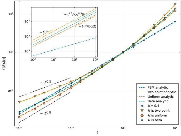
Figure 1: Mean squared displacement of FBMREs with two-point, uniform and beta distributions of the Hurst exponent calculated analytically by using the results from Section III (different lines), and by means of Monte Carlo simulations (different markers). For the two-point distribution $H_{1}=0.25$, $H=0.75$ with $p=0.5$, uniform is distributed on $(0.25,0.75)$, and beta is distributed on (0.25,0.75) with $\alpha=\beta=0.5$. The reference blue line and blue diamond markers correspond to FBM with $H=0.4$. The inset depicts the analytical behaviour for longer times and the asymptotics are plotted next to the relevant cases.

We now concentrate on two distributions, which we believe, can serve as the most important generic cases, namely the two-point and beta. The two-point distribution has the probability masses $p$ and $1-p$ at $H_{1}=0.25$ and $H_{2}=0.75$, respectively. The beta distribution is defined on the same range $(0.25,0.75)$. Further, for the two-point distribution we analyse three cases, namely $p=0.1$ (’almost’ superdiffusion), $p=0.5$ (intermediate case), and $p=0.9$ (’almost’ subdiffusion). Similarly, for the beta distribution we select three pairs of parameters $\alpha=0.7$, $\beta=0.3$; $\alpha=0.5$. $\beta=0.5$, and $\alpha=0.3$, $\beta=0.7$. The PDFs for the three selected cases are presented in Figure 2. From here one can see that for $\alpha=0.7$ and $\beta=0.3$ the distribution is skewed to the right (the same type of skewness as for the two-point distribution with $p=0.1$); for $\alpha=0.5$ and $\beta=0.5$ the distribution is symmetric around its mean $H=0.5$ (similar to two-point distribution with $p=0.5$), and for $\alpha=0.3$ and $\beta=0.7$ the distribution is skewed to the left (as for the two-point distribution with $p=0.9$).

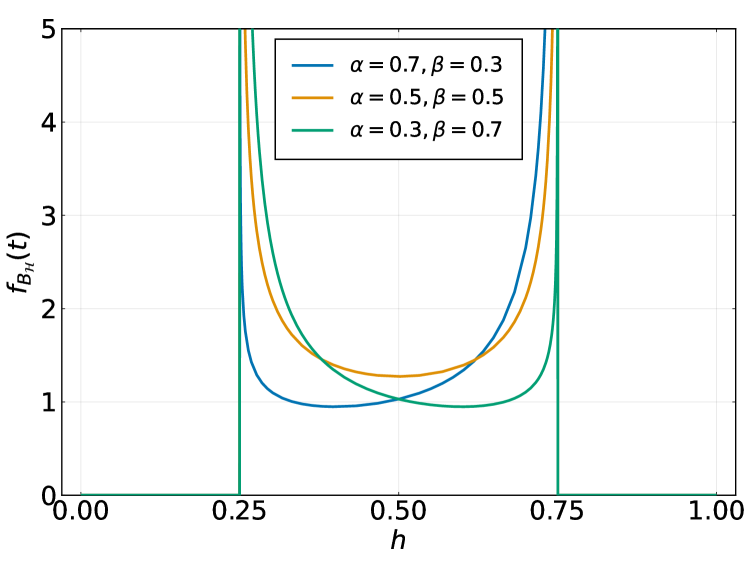
Figure 2: Probability density function for the beta distribution defined on the interval $(0.25,0.75)$ for three different pairs of the parameters: $\alpha=0.7$ and $\beta=0.3$ (blue line); $\alpha=0.5$ and $\beta=0.5$ (orange line); $\alpha=0.3$ and $\beta=0.7$ (green line).

In Figure 3 we depict PDFs of the FBMREs for the two distributions of the Hurst parameter, and PDFs of the FBM for $H=0.25$ and $H=0.75$, for two time points: $t=1$ and $t=10$. The parameters of the distributions are the same as used in Figure 1 for the intermediate case $p=0.5$. In Figures 3(a)-(b) the behaviour of the two-point distribution is shown. We observe that for short time $t=1$ the center of the distribution resembles the PDF of FBM with $H=0.75$, while the tails coincide with those of FBM with $H=0.25$. For long time $t=10$ situation is quite opposite: the tails correspond to FBM with $H=0.75$ and the distribution center to FBM with $H=0.25$. In Figures 3(c)-(d) the beta distribution case is presented. The most striking difference from the two-point distribution case is the fact the tails are no longer close to Gaussian and they rather resemble an exponential decay. This is due to the fact that for the two-point distribution, the FBMRE follows a mixture of two normal laws, whereas for the beta distribution the resulting distribution structure is more complex and leads to exponential-like tails.

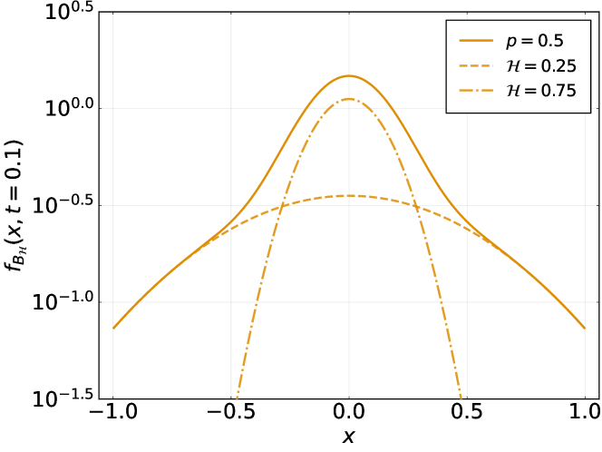
(a)

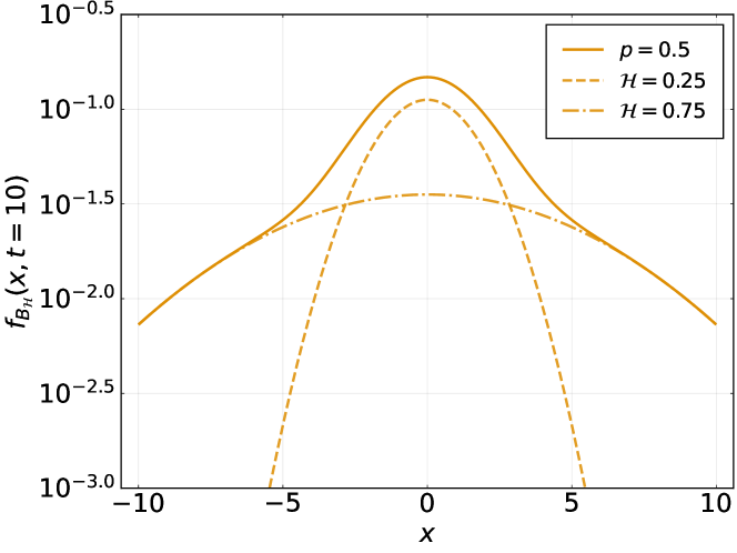
(b)

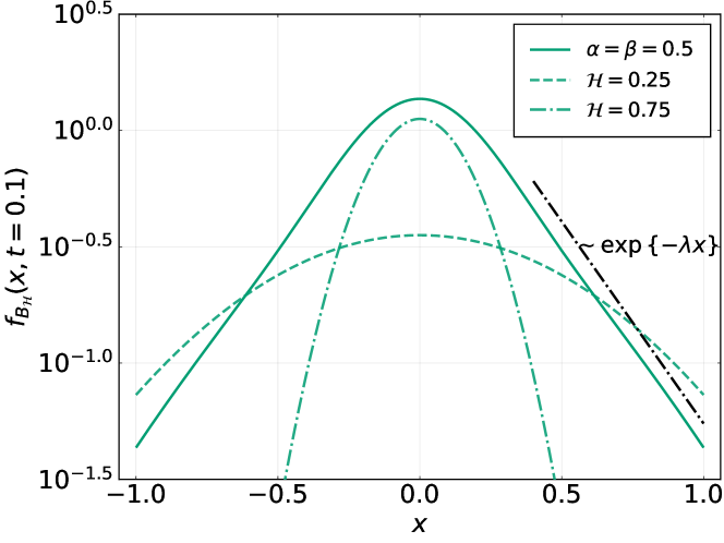
(c)

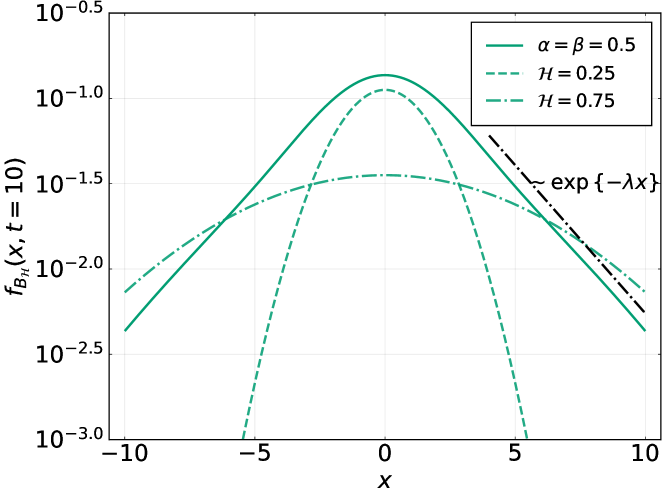
(d)

Figure 3: Probability density function of FBMREs for two-point (top panels) and beta (bottom panels) distributions of the Hurst parameter for two time points: $t=1$ (left panels) and $t=10$ (right panels) (solid lines). The parameters of the distributions are the same as used in Figure 1. Dashed green lines correspond to FBM with $H=0.25$ and dot-dashed green lines to FBM with $H=0.75$. Dot-dashed black lines represent exponential decay of the tails of the distribution, with $\lambda=4$ (bottom left panel) and $\lambda=0.4$ (bottom right panel).

In Figure 4, the long-time behaviour of the ACVFs for the two distributions is depicted as the functions of the lag $\tau$. For the two-point distribution, see Figure 4(a), we can see that the probability masses assigned to the points $H_{1}=0.25$, $H_{2}=0.75$ have a significant impact on the behaviour of ACVF, namely if the mass assigned to $H_{1}=0.25$ is small ($p=0.1$), then the ACVF is positive (apart from the very small lags), which corresponds to the superdiffusive (persistent) case. In contrast, for $p=0.9$ the ACVF is negative and converges to zero which matches the subdiffusive (antipersistent) case. For the probability mass $p=0.5$, the situation is intermediate, namely the ACVF starts with negative values, at lag around $30$ ACVF crosses the zero level and then it is positive, hence the process clearly performs the persistence transition. A similar behaviour can be also observed in Figure 4(b) for the beta distribution defined on the interval $(0.25,0.75)$ for three corresponding choices of the distribution parameters. When the parameters $\alpha$ and $\beta$ are equal then the persistence transition is again clearly visible.

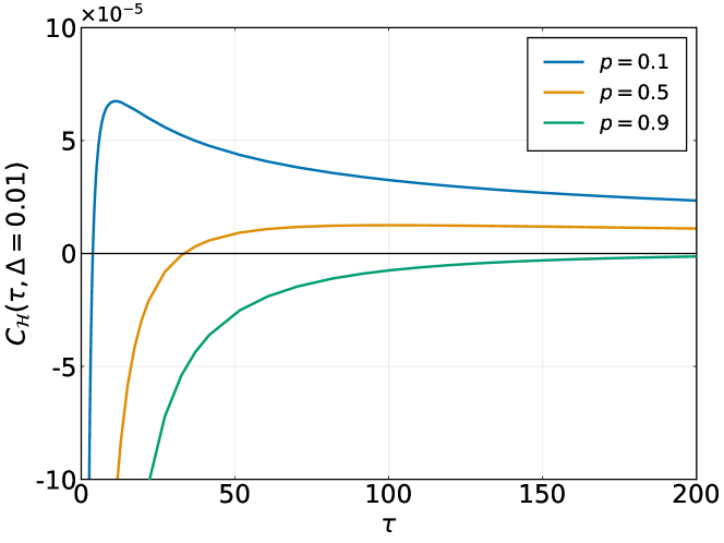
(a)

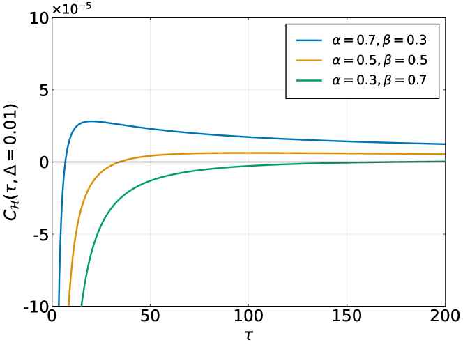
(b)

Figure 4: Long-time ACVF $C_{\mathcal{H}}(\tau,\Delta)$ of the FBMRE increments for $\Delta=0.01$ with two-point (panel (a)) and beta (panel (b)) distributions of the Hurst exponent. For the two-point distribution the parameters are $H_{1}=0.25$, $H_{2}=0.75$, and $p=0.1$ (blue line), $0.5$ (orange line), $0.9$ (green line). The beta distribution is defined on $(0.25,0.75)$ with parameters $\alpha=0.7$, $\beta=0.3$ (blue line), $\alpha=0.5$, $\beta=0.5$ (orange line), and $\alpha=0.3$, $\beta=0.7$ (green line). For clarity of the presentation we do not plot the ACVF for lag equal to zero which is the variance of the increment process.

To gain more insight into the persistence transition observed for the two-point and beta distributions, we analyse in detail the ACVFs $C_{\mathcal{H}}(\tau,\Delta)$ in Figures 5 and 6 for two different lag values $\tau=0.1$ and $\tau=10$ which differ by two orders of magnitude. We can see in Figure 5, which corresponds to the two-point distribution, that the ACVF behaviour is different for small and large lags. For smaller lags, as probability mass $p$ at $H_{1}$ increases, the $H_{2}$ value becomes irrelevant, i.e. the carpets consist of vertical stripes. The ACVF values are predominantly positive for $p=0.1$, and when the probability mass increases the negative values start to dominate. In contrast, for the larger lags, the plots resemble patches of horizontal stripes especially for small probability masses at $H_{1}$, i.e. the $H_{1}$ values becomes irrelevant. We also notice that the ACVF is always non-negative in this case. Finally, we note that for $H_{1}=H_{2}=0.5$ with $p=0.5$ we recover the Brownian motion case and the ACVF is equal to zero.

In Figure 6 we present the behaviour of the ACVF for the beta distribution. It is similar to that for the two-point distribution depicted in Figure 5, except for the smaller lag when the $H_{2}$ parameter always has some effect on the ACVF (observed stripes are not perfectly vertical).

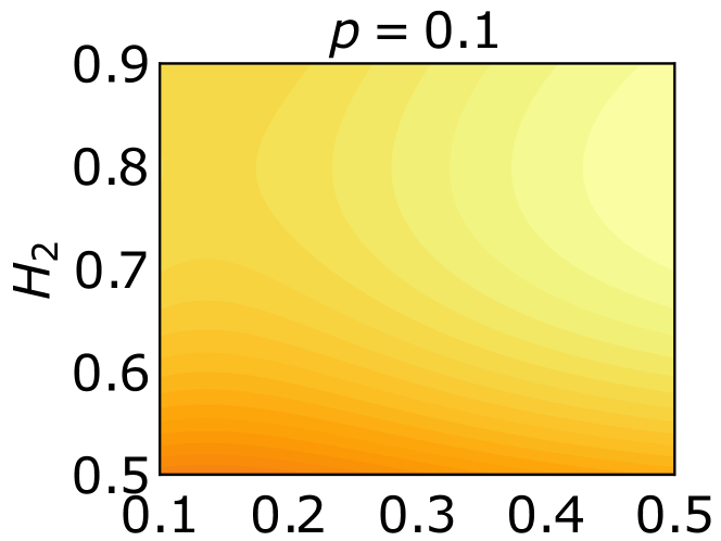
(a)

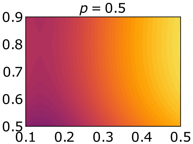
(b)

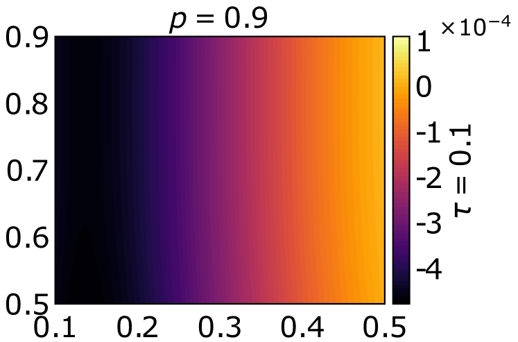
(c)

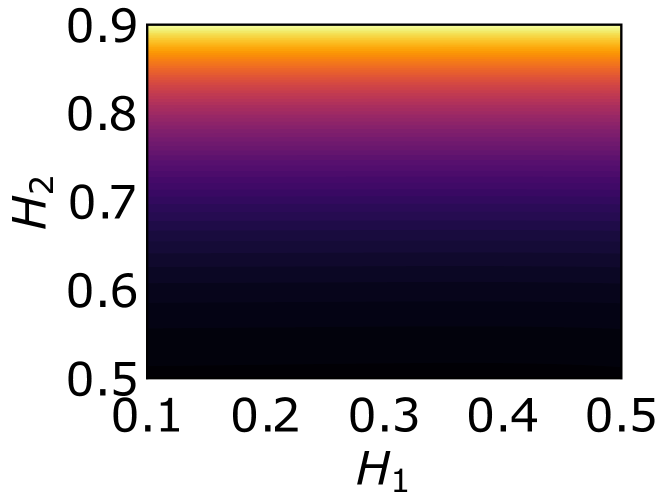
(d)

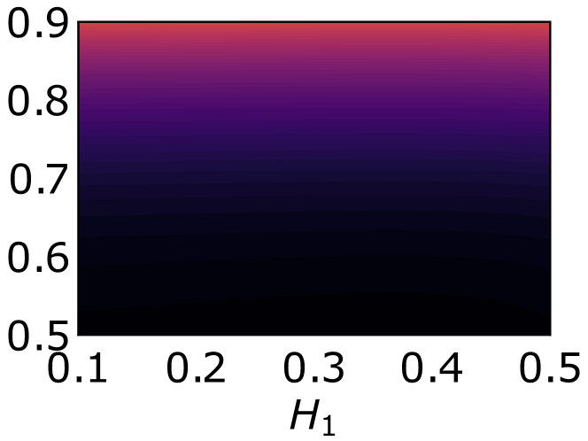
(e)

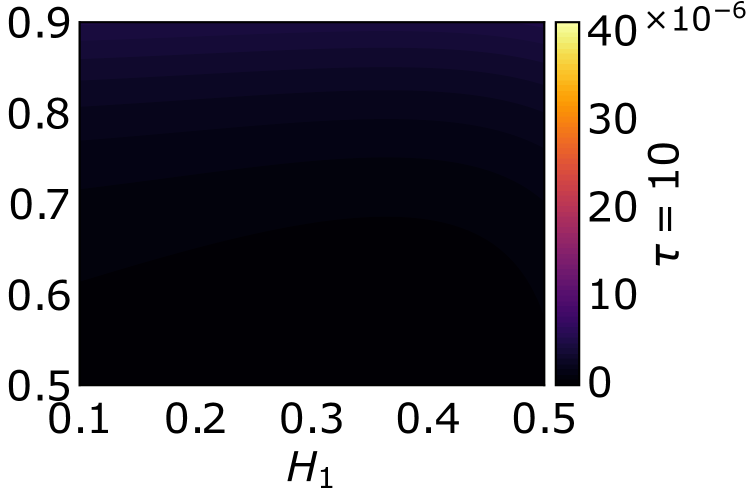
(f)

Figure 5: Carpet plots of ACVFs for the FBMRE increments for $\Delta=0.01$ with the two-point distribution of the Hurst exponent defined on the interval $(H_{1},H_{2})$ for the three cases of parameter $p=0.1$ (left panels), $0.5$ (middle panels), and $0.9$ (right panels), and for two different lags $\tau=0.1$ (top panels) and $\tau=10$ (bottom panels).

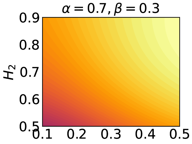
(a)

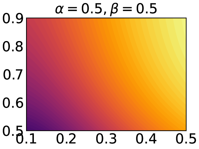
(b)

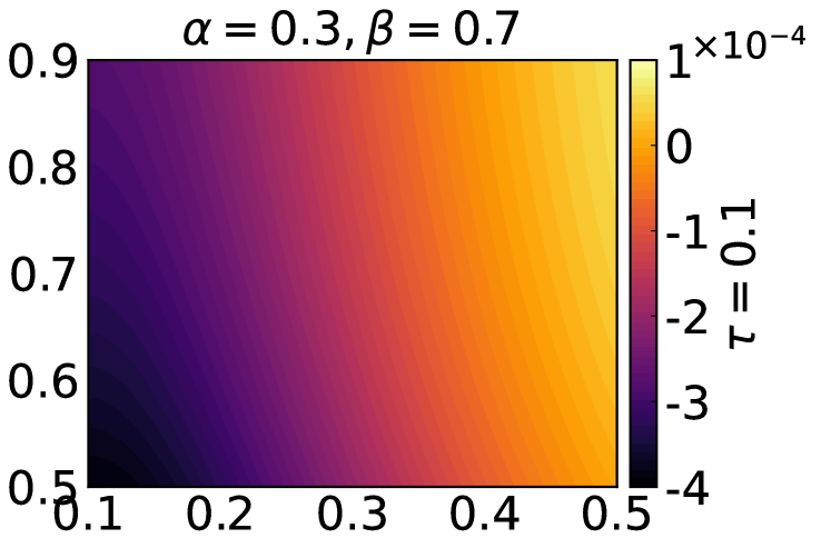
(c)

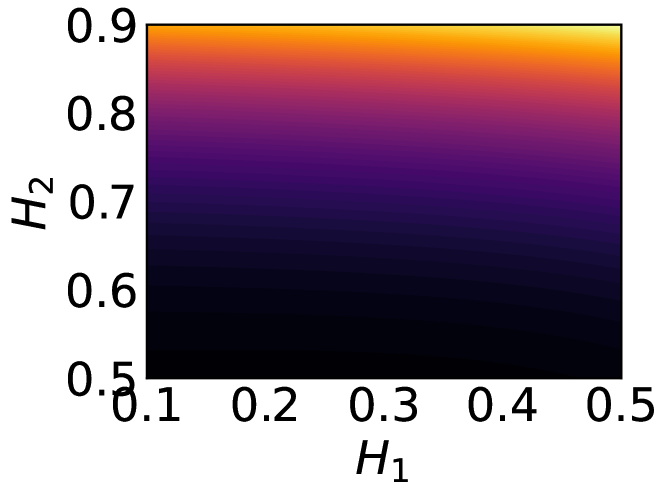
(d)

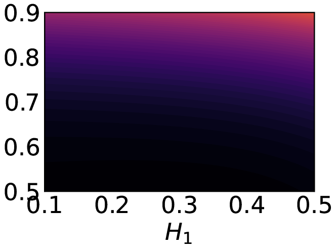
(e)

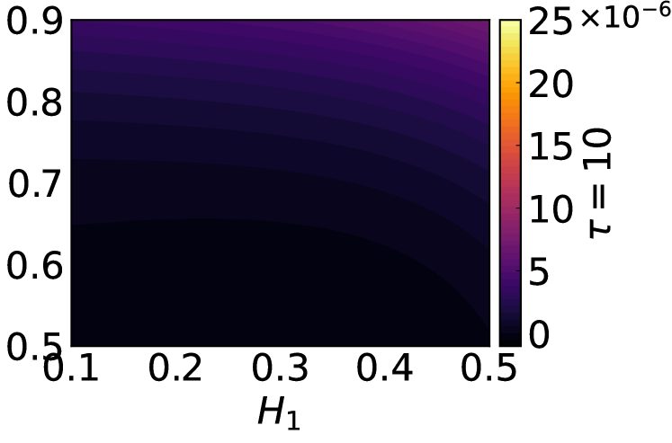
(f)

Figure 6: Carpet plots of ACVFs for the FBMRE increments for $\Delta=0.01$ with the beta distribution of the Hurst exponent defined on the interval $(H_{1},H_{2})$, for three different cases $\alpha=0.7$, $\beta=0.3$ (left panels), $\alpha=0.5$, $\beta=0.5$ (middle panels), and $\alpha=0.3$, $\beta=0.7$ (right panels), and for two different lags $\tau=0.1$ (top panels) and $\tau=10$ (bottom panels).

Finally, for the two considered distributions we calculate the persistence transition lags and present them in the form of carpet plots in Figures 7 and 8. We can observe that the waiting times for the transition are similar for the two-point and beta distributions.

(a)

(b)

(c)

Figure 7: Carpet plots of the persistence transition lags for the two-point distribution of the Hurst index defined on the interval $(H_{1},H_{2})$ and $\Delta=0.01$, for three cases: $p=0.1$ (panel (a)), $0.5$ (panel (b)), and $0.9$ (panel (c)).

(a)

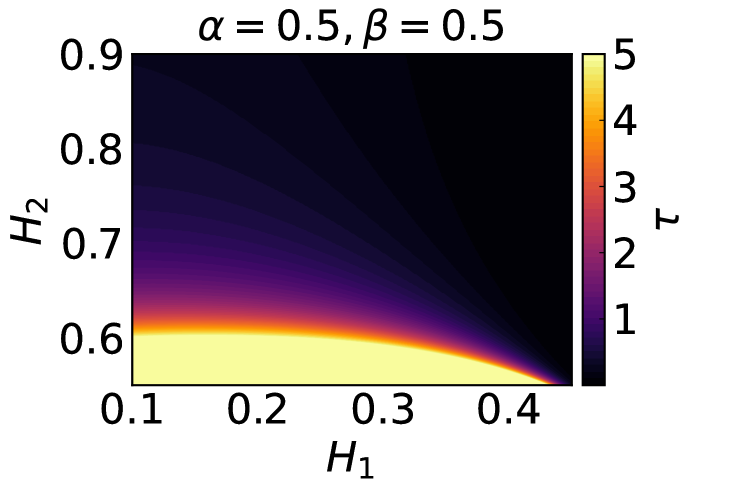
(b)

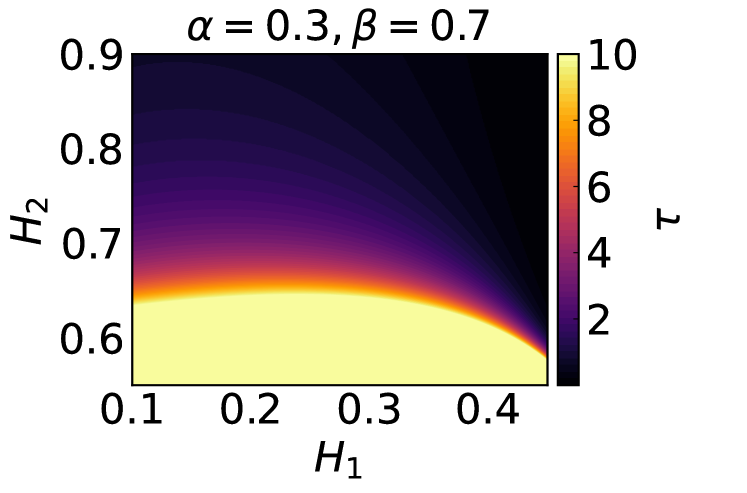
(c)

Figure 8: Carpet plots of the persistence transition lags for the beta distribution of the Hurst exponent defined on the interval $(H_{1},H_{2})$ and $\Delta=0.01$, for three cases: $\alpha=0.7$, $\beta=0.3$ (panel (a)), $\alpha=0.5$, $\beta=0.5$ (panel (b)), and $\alpha=0.3$, $\beta=0.7$ (panel (c)).

To sum up, numerical experiments show that the FBMRE exhibits distinct properties. First, it leads to accelerating diffusion, namely the MSD exponent increases in time, see Figure 1. Second, the distribution of the process increments is not Gaussian: for the two-point distribution of the Hurst exponent it follows a mixture of two Gaussian laws and for the beta distribution the tails become exponential (see Figure 3). Third, the increment process can show persistence transition, namely its ACVF switches sign at some lag. This behavior is presented in Figure 4 and is further studied in Figures 5-8.

V Discussion and conclusion

In this section, we discuss several issues related to the theory of FBMRE and its further extensions which we suppose to address in future studies.

V.1 Beta distribution fits empirical PDFs of the Hurst exponent

In single particle tracking experiments with tracers in mucin hydrogels under acidic conditions ($pH=2$), FBM was found to be the most likely model for majority of the trajectories [20]. Further, Bayesian inference at the single trajectory level revealed trajectory to trajectory fluctuations in the estimated Hurst exponent. Such variations were found to be consistent with estimates from the TAMSD for each trajectory. In Figure 9 we show that the distribution of Hurst exponents estimated using Bayesian inference in Ref.[20] is consistent with a beta distribution. The maximum likelihood estimators are $\alpha=3.37$ and $\beta=2.1$. We also performed the Kolmogorov-Smirnov goodness-of-fit test [49] for the beta distribution with the estimated parameters and obtained the $p$-value equal to $0.2557$ which does not lead to rejection of the underlying beta distribution hypothesis with $5\%$ significance level.

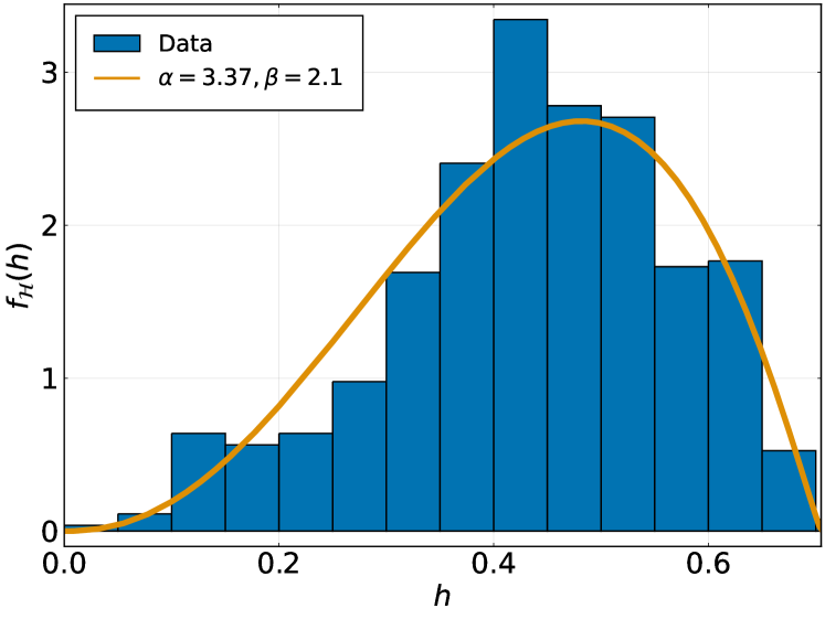
Figure 9: Histogram of Hurst exponents estimated using Bayesian inference in Ref.[20] for tracers tracked in mucin hydrogels and the fitted probability density function of the beta distribution. The data set corresponds to $N=532$ two-dimensional trajectories of tracers tracked at $pH=2$ and zero salt concentration.

Another example comes from the experiment with tracer particles in mammalian cells[21, 22]. The experimental observations can be described by FBM with the marked heterogeneity in individual particle trajectories. In Figure 10 we demonstrate that the distribution of Hurst exponents is consistent with the beta distribution with $\alpha=1.58$ and $\beta=3.88$. The Kolmogorov-Smirnov goodness-of-fit test for beta distribution with the estimated parameters gives the $p$-value equal to $0.178$.

The two presented examples show usefulness of beta distribution in fitting and analyzing experimental data with Hurst exponent randomly changing from trajectory to trajectory. This also justifies our choice of beta distribution for the analytical studies. It would be of interest to provide similar analysis with the empirical distributions presented in Refs.[17, 18, 33, 39].

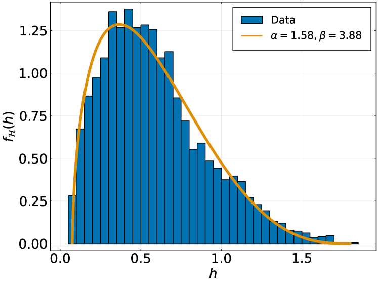
Figure 10: Histogram of Hurst exponents estimated using MSD approach in Ref.[21, 22] for tracer particles in the cytoplasm of mammalian cells and the fitted probability density function of the beta distribution. The data set corresponds to $N=3834$ trajectories.

V.2 Is the Hurst exponent a constant or a random variable?

The Hurst exponent can be estimated from experimental or simulated data using different statistics such as e.g., R/S statistic, rescaled variance statistic, detrended fluctuation analysis or TAMSD [50, 51, 52, 53, 54, 55]. As a result, one obtains the value of the estimator $\hat{H}$ that is a random variable. The papers [53, 50] discuss the sample distribution of $\hat{H}$ while the analytical derivation of the distribution of $\hat{H}$ for a finite number of data points was provided in [54] by using TAMSD statistic for FBM. How can one distinguish between two different sources of randomness of the estimated Hurst exponent, namely finiteness of the data set and random change from trajectory to trajectory? This issue points to the need to introduce effective tools for distinguishing between these two cases. One idea could be to measure the MSD as a function of time which should demonstrate either linear or convex behavior (in log-log scale) in time for a single or random Hurst exponent, respectively. Another proposition is to compare the sample distribution obtained for the estimated Hurst exponent by using TAMSD statistic with the analytical distribution presented in [54]. Alternatively, the uncertainty in the estimated value of the parameter due to finiteness of the data can be quantified using single trajectory analysis methods such as Bayesian inference and machine learning. Bayesian inference provides with the posterior distribution of the parameters—for example the Hurst exponent—given the data and a prior on the parameters. The variance of such a posterior distribution then quantifies the uncertainty in the estimated value of the parameter. Performing Bayesian parameter estimation on simulated trajectories of different lengths can then quantify the uncertainty in the estimation due to the finite length of trajectories. Such studies have been conducted in, for example, Refs.[56, 57, 58]. The quantification of uncertainty due to finite number of data points has also been done using machine learning approaches [59].

V.3 Is the Hurst exponent a random variable or a random process?

Recent studies of the random intracellular motions point to the necessity of going beyond the FBMRE concept to explain the highly heterogeneous transport of structures inside living cells [33, 39, 38]. The MPRE allowing the Hurst parameter to vary stochastically in time [34] is a natural extension of FBMRE, and its basic mathematical properties are worth to be explored, similar to how it is done in the present paper. We also note that the two processes, FBMRE and MPRE, can be distinguished by analyzing their TAMSD, namely while FBMRE is a mean-squared ergodic process, the MPRE does not exhibit this property.

V.4 Mimicking heterogeneous environment with random Hurst exponent

The anomalous transport in biological media has largely been attributed to heterogeneity [16] which itself can arise from two sources: (a) the spatially heterogeneous macromolecular crowding in, for instance, the cell cytoplasm and/or (b) heterogeneity in the shape and size of different constituents, such as proteins and lipids, of a biological cell. The former source may correspond to having local patches in a viscoelastic environment where a synthetic particle of known shape and size—tracked for a finite time such that it diffuses within the patch during this period—diffuses with a constant Hurst exponent. Another particle in a neighbouring patch in the medium might diffuse with a different Hurst exponent. Thus, the random Hurst exponents extracted from the trajectories of such particles mimic the heterogeneous environment. However, when the tracked particles are cellular constituents, such as proteins, the ensemble itself might be heterogeneous (non-identical particles), potentially giving rise to trajectory to trajectory fluctuations in the estimates of the Hurst exponent. Besides, such fluctuations may also arise from the superimposition of active processes on the motion of tracked particles [18]. How to disentangle the two potential sources of heterogeneity—listed above as (a) and (b)—is an interesting research question which might be investigated experimentally. We note here that the authors in Ref.[60] explained the dynamics of a transmembrane protein (DC-SIGN) on living-cell membranes by considering local patches of fixed diffusivity, which mimicked the heterogeneity of the cell membranes.

FBMRE presented in this article describes the scenarios of heterogeneity discussed in the preceding paragraph. However, the scenarios can be further complicated if, for example, the local patches with fixed Hurst exponent are small such that a tracked particle transitions multiple times between such patches with different Hurst exponents during the total experimental time period. Moreover, when the tracked particle is a cell-constituent such as a protein, it may change shape and size during its dynamics. Furthermore, given that a biological cell is dynamic, the cellular environment itself might change during the experiment. These scenarios would call for a generalization of FBMRE to include a Hurst exponent which is stochastic along an individual trajectory. We are currently exploring such generalizations as a follow-up of the present article.

In summary, in this paper we study the basic mathematical properties of the fractional Brownian motion with the Hurst exponent randomly changing from trajectory to trajectory. To the best of our knowledge, this is the first paper in the literature providing such complex analysis of the process with random Hurst exponent. Specifically, we provide general expressions for the probability density function, the $q-$th moment (including mean squared displacement) and autocovariance function for the increment process. We derive explicit results for three generic distributions of random Hurst exponent, namely, two-point, uniform and beta distributions. Our analytical and numerical analyses reveal two effects which are the hallmarks of the process, namely accelerating diffusion and persistence transition. Taking into account that three generic types of the distributions considered in our paper exhibit qualitatively similar properties, we conclude that these two effects are quite common for FBMRE. Our analytical expressions quantify and illustrate how they arise, and our simulations validate them. The presented results pave the way to a consistent mathematical and statistical description of fractional motions in complex heterogeneous environment. We hope that this paper will be of interest to researchers working not only in the field of biology but also climate, hydrology and financial markets where FBM is one of the canonical processes. Moreover, we hope to inspire experimentalists to test the two phenomena we discovered. Given the number of recent experiments which have reported FBMRE, we believe that the mathematical framework and the numerical methods we present are of significant potential utility.

Data Availability

The data that support the findings of this study are available from the corresponding author upon reasonable request.

Appendix A Derivation of $A_{H}$ prefactor

Starting with the integral representation of FBM as given in Eq. (1), we get

$$\mathbb{E}\left(B_{H}^{2}(t)\right) = A^{2}_{H}t^{2H}\Bigg{\{}\frac{1}{2H}$$ (45)

$$+ \int_{0}^{\infty}\left[(1+u)^{H-1/2}-u^{H-1/2}\right]^{2}du\Bigg{\}}.\quad$$

The formula in parentheses can be written as

$$\Bigg{\{}\ldots\Bigg{\}} = \frac{1}{2H}+\lim_{a\to\infty}\int_{0}^{a}(1+u)^{2H-1}du$$ (46)

$$+ \lim_{a\to\infty}\int_{0}^{a}\;u^{2H-1}du$$

$$- 2\lim_{a\to\infty}\int_{0}^{a}\;u^{2H-1}\left(1+\frac{1}{u}\right)^{H-1/2}du$$

$$= \lim_{a\to\infty}\left[\frac{a^{2H}}{H}+a^{2H-1}-2I(a,H)\right],$$

where

$$I(a,H)=\int_{0}^{a}\;u^{2H-1}\left(1+\frac{1}{u}\right)^{H-1/2}du$$ (47)

is the incomplete beta function.

Now, we take the integral $I(a,H)$ twice by parts in order to extract the terms that diverge at $a\to\infty$,

$$I(a,H) = \frac{a^{2H}}{2H}+\frac{a^{2H-1}}{2}$$ (48)

$$+ \frac{H-3/2}{4H}\int_{0}^{a}\;u^{2H-3}\left(1+\frac{1}{u}\right)^{H-5/2}du.\quad$$

Note that the integral in Eq. (48) converges at $a\to\infty$. After plugging Eq. (48) into Eq. (46) we obtain

$$\Bigg{\{}\ldots\Bigg{\}} = \frac{3/2-H}{2H}\int_{0}^{\infty}\frac{u^{H-1/2}}{(1+u)^{5/2-H}}du$$ (49)

$$= \frac{3/2-H}{2H}\mathbb{B}\left(H+\frac{1}{2},2-2H\right),\quad$$

where $\mathbb{B}(x,y)$ is the beta function defined in Eq. (37). Finally, we plug Eq. (49) into Eq. (45) to obtain

$$\mathbb{E}\left(B_{H}^{2}(t)\right)=A^{2}_{H}t^{2H}\frac{\Gamma^{2}(H+1/2)}{\Gamma(1+2H)\sin\left(\pi H\right)}.$$ (50)

Imposing $\mathbb{E}\left(B_{H}^{2}(t)\right)=t^{2H}$ gives the expression for $A_{H}$,

$$A_{H}=\frac{\sqrt{\Gamma(1+2H)\sin\left(\pi H\right)}}{\Gamma(H+1/2)}.$$ (51)

Appendix B Asymptotics of ACVF in case of uniform distribution of the random Hurst exponent

For small $\tau/\Delta\ll 1$ we have the following asymptotic behavior for ACVF $C_{{\mathcal{H}}}(\tau,\Delta)$

$$C_{{\mathcal{H}}}(\tau,\Delta) \sim \frac{1}{(H_{2}-H_{1})\log(\Delta)}\Bigg{[}\Delta^{2H_{2}}\left(1-\left(\frac{\tau}{\Delta}\right)^{2H_{2}}\right)$$ (52)

$$- \Delta^{2H_{1}}\left(1-\left(\frac{\tau}{\Delta}\right)^{2H_{1}}\right)\Bigg{]}.$$

Note that $C_{\mathcal{H}}(0,\Delta)$ is always positive, as it should be. For large $\tau/\Delta\gg 1$ the Eq. (33) gets a simpler form if in addition we require one of the following conditions, namely either a) $\Delta\ll\tau\ll 1$ or b) $\tau\gg\Delta\gg 1$. Then we get

$$C_{{\mathcal{H}}}(\tau,\Delta) \sim \frac{\Delta^{2}}{(H_{2}-H_{1})\log(\tau)}\left(H_{2}(2H_{2}-1)\tau^{2(H_{2}-1)}\right.$$ (53)

$$- \left.H_{1}(2H_{1}-1)\tau^{2(H_{1}-1)}\right)+\delta C_{\mathcal{H}},$$

and the correction term $\delta C_{\mathcal{H}}$ contains additional prefactor $1/\log(\tau)$.

Appendix C Beta distribution on the interval $(0,1)$ of the random Hurst exponent

The PDF of beta distribution on the interval $(0,1)$ with parameters $\alpha>0$ and $\beta>0$ reads

$$f_{\mathcal{H}}(h)=\frac{h^{\alpha-1}(1-h)^{\beta-1}}{\mathbb{B}(\alpha,\beta)}{I}_{h\in(0,1)}.$$ (54)

The MFG is given by

$$M_{\mathcal{H}}(s)={}_{1}F_{1}(\alpha,\alpha+\beta,s),$$ (55)

where $\mathbb{B}(\alpha,\beta)$ is the beta function defined in Eq. (37), and ${}_{1}F_{1}(\cdot,\cdot,\cdot)$ is a confluent hypergeometric function (Kummer function)

$${}_{1}F_{1}(a,b,z)=\sum_{n=0}^{\infty}\frac{(a)_{n}}{(b)_{n}}\frac{z^{n}}{n!}=1+\frac{a}{b}z+\cdots.$$ (56)

In the formula above $a,b$ are positive constants, $z\in\mathbb{R}$, and $(a)_{n}$ is the Pochhammer symbol, i.e. $(a)_{0}=1$ and $(a)_{n}=a(a+1)(a+2)\ldots(a+n-1)$ for $n\geq 1$.

Using Eq. (7) we obtain the PDF $f_{B_{\mathcal{H}}}(x,t)$,

$$f_{B_{\mathcal{H}}}(x,t) = \frac{1}{\mathbb{B}(\alpha,\beta)}$$

$$\times \int_{0}^{1}\frac{h^{\alpha-1}(1-h)^{\beta-1}}{\sqrt{2\pi t^{2h}}}\exp\left\{\frac{-x^{2}}{2t^{2h}}\right\}dh.$$

With the use of Eq. (8) the MSD takes the form

$$\mathbb{E}\left(B_{\mathcal{H}}^{2}(t)\right) = {}_{1}F_{1}(\alpha,\alpha+\beta,2\log(t)).$$ (58)

Notice that for large $z$, except when $a=0,-1,\ldots$ (polynomial cases), the confluent hypergeometric function given in (56) behaves as

$${}_{1}F_{1}(a,b,z)\sim\frac{\Gamma(b)e^{z}z^{a-b}}{\Gamma(a)}.$$ (59)

Thus, using the Kummer’s transformation for the confluent hypergeometric function

$${}_{1}F_{1}(a,b,z)=e^{z}{}_{1}F_{1}(b-a,b,-z),$$ (60)

we obtain the asymptotics of MSD for short times

$$\mathbb{E}\left(B_{\mathcal{H}}^{2}(t)\right) \sim \frac{\Gamma(\alpha+\beta)}{\Gamma(\beta)}\frac{1}{(2\log(1/t))^{\alpha}},$$ (61)

whereas for long times we have

$$\mathbb{E}\left(B_{\mathcal{H}}^{2}(t)\right) \sim \frac{\Gamma(\alpha+\beta)}{\Gamma(\alpha)}\frac{t^{2}}{(2\log(t))^{\beta}}.$$ (62)

Using Eq. (13) and the MGF (55) we obtain the ACVF for $\{b_{\mathcal{H}}^{\Delta}(t)\}$,

$$C_{{\mathcal{H}}}(\tau,\Delta) = \frac{1}{2}{}_{1}F_{1}(\alpha,\alpha+\beta,2\log(\tau+\Delta))$$ (63)

$$+ \frac{1}{2}{}_{1}F_{1}(\alpha,\alpha+\beta,2\log(|\tau-\Delta|))$$

$$- {}_{1}F_{1}(\alpha,\alpha+\beta,2\log(\tau)).$$

Appendix D Asymptotics of ACVF in case of beta distribution on the interval $[H_{1},H_{2}]$ of the random Hurst exponent

For asymptotic behavior of ACVF $C_{\mathcal{H}}(\tau,\Delta)$, Eq. (44), at $\tau/\Delta\ll 1$ we get

$$C_{\mathcal{H}}(\tau,\Delta) \sim \Delta^{2H_{1}}\Bigg{[}{}_{1}F_{1}\left(\alpha,\alpha+\beta,2(H_{2}-H_{1})\log\Delta\right)$$

$$- \left(\frac{\tau}{\Delta}\right)^{2H_{1}}{}_{1}F_{1}\left(\alpha,\alpha+\beta,2(H_{2}-H_{1})\log\tau\right)\Bigg{]}.$$

This result acquires an elegant form in two limit cases, namely a) $\tau\ll\Delta\ll 1$, where

$$C_{\mathcal{H}}(\tau,\Delta) \sim \frac{\Gamma(\alpha+\beta)}{\Gamma(\beta)[2(H_{2}-H_{1})]^{\alpha}}\frac{\Delta^{2H_{1}}}{\log^{\alpha}(1/\Delta)}$$ (65)

$$\times \Bigg{[}1-\left(\frac{\tau}{\Delta}\right)^{2H_{1}}\frac{\log^{\alpha}(1/\Delta)}{\log^{\alpha}(1/\tau)}\Bigg{]}$$

and b) $\Delta\gg\tau\gg 1$ where

$$C_{\mathcal{H}}(\tau,\Delta) \sim \frac{\Gamma(\alpha+\beta)}{\Gamma(\beta)[2(H_{2}-H_{1})]^{\beta}}\frac{\Delta^{2H_{2}}}{\log^{\beta}(\Delta)}$$ (66)

$$\times \Bigg{[}1-\left(\frac{\tau}{\Delta}\right)^{2H_{2}}\frac{\log^{\beta}(\Delta)}{\log^{\beta}(\tau)}\Bigg{]}.$$

At $\tau/\Delta\gg 1$ the asymptotics of ACVF reads

$$C_{\mathcal{H}}(\tau,\Delta) \sim \frac{\Delta^{2}}{\tau^{2-2H_{1}}}\Bigg{[}H_{1}(2H_{1}-1){}_{1}F_{1}\left(\alpha,\alpha+\beta,2(H_{2}-H_{1})\log\tau\right)$$ (67)

$$+ \frac{(H_{2}-H_{1})(2H_{1}-1)\alpha}{\alpha+\beta}{}_{1}F_{1}\left(\alpha+1,\alpha+\beta+1,2(H_{2}-H_{1})\log\tau\right)$$

$$+ \frac{(H_{2}-H_{1})^{2}\alpha(\alpha+1)}{(\alpha+\beta)(\alpha+\beta+1)}{}_{1}F_{1}\left(\alpha+2,\alpha+\beta+2,2(H_{2}-H_{1})\log\tau\right)\Bigg{]}.$$

References

- Einstein [1905] A. Einstein, “Über die von der molekularkinetischen Theorie der Wärme geforderte Bewegung von in ruhenden Flüssigkeiten suspendierten Teilchen,” Ann. Phys. 322, 549 (1905).
- Sutherland [1905] W. Sutherland, “A dynamical theory of diffusion for non-electrolytes and the molecular mass of albumin,” Philos. Mag. 9, 781 (1905).
- von Smoluchowski [1906] M. von Smoluchowski, “Zur kinetischen Theorie der Brownschen Molekularbewegung und der Suspensionen,” Ann. Phys. 21, 756 (1906).
- Langevin [1908] P. Langevin, “Sur la théorie du mouvement brownien,” C. R. Acad. Sci. (Paris) 530, 146 (1908).
- Gnedenko and Kolmogorov [1954] B. V. Gnedenko and A. N. Kolmogorov, Limit Distributions for Sums of Independent Random Variables (Gostekhizdat, Moscow, 1949, Eng. transl. Addison–Wesley, Boston, 1954).
- Donsker [1952] M. D. Donsker, “Justification and Extension of Doob’s Heuristic Approach to the Kolmogorov- Smirnov Theorems,” The Annals of Mathematical Statistics 23, 277 (1952).
- Bouchaud and Georges [1990] J.-P. Bouchaud and A. Georges, “Anomalous diffusion in disordered media: statistical mechanisms, models and physical applications,” Physics Reports 195, 127 (1990).
- Klages, Radons, and Sokolov [eds.] R. Klages, G. Radons, and I. M. Sokolov (eds.), Anomalous transport : foundations and applications (Wiley-VCH, Berlin, 2008).
- Sokolov [2012] I. M. Sokolov, “Models of anomalous diffusion in crowded environments,” Soft Matter 8, 9043 (2012).
- Metzler et al. [2014] R. Metzler, J. H. Jeon, A. G. Cherstvy, and E. Barkai, “Anomalous diffusion models and their properties: non-stationarity, non-ergodicity, and ageing at the centenary of single particle tracking,” Physical Chemistry Chemical Physics 16, 24128 (2014).
- Kolmogorov [1940] A. N. Kolmogorov, “Wienersche Spiralen und einige andere interessante Kurven in Hilbertscen Raum,” C.R. (Doklady) Acad. Sci. URSS (NS) 26, 115 (1940).
- Mandelbrot and Ness [1968] B. B. Mandelbrot and J. W. V. Ness, “Fractional Brownian Motions, Fractional Noises and Applications,” SIAM Review 10, 422 (1968).
- Doukhan, Oppenheim, and [Eds.] P. Doukhan, G. Oppenheim, and M. S. T. (Eds.), Theory and applications of long-range dependence (Birkhóauser Boston, Inc., Boston, 2003).
- Beran et al. [2016] J. Beran, Y. Feng, S. Ghosh, and R. Kulik, Long-Memory Processes (Springer, 2016).
- Ernst et al. [2012] D. Ernst, M. Hellmann, J. Köhler, and M. Weiss, “Fractional Brownian motion in crowded fluids,” Soft Matter 8, 4886 (2012).
- Höfling and Franosch [2013] F. Höfling and T. Franosch, “Anomalous transport in the crowded world of biological cells,” Rep. Prog. Phys. 76, 046602 (2013).
- Sadoon and Wang [2018] A. A. Sadoon and Y. Wang, “Anomalous, non-Gaussian, viscoelastic, and age-dependent dynamics of histonelike nucleoid-structuring proteins in live escherichia coli,” Physical Review E 98, 042411 (2018).
- Benelli and Weiss [2021] R. Benelli and M. Weiss, “From sub-to superdiffusion: Fractional Brownian motion of membraneless organelles in early C. elegans embryos,” New Journal of Physics 23, 063072 (2021).
- Speckner and Weiss [2021] K. Speckner and M. Weiss, “Single-particle tracking reveals anti-persistent subdiffusion in cell extracts,” Entropy 23, 892 (2021).
- Cherstvy et al. [2019] A. G. Cherstvy, S. Thapa, C. E. Wagner, and R. Metzler, “Non-Gaussian, non-ergodic, and non-Fickian diffusion of tracers in mucin hydrogels,” Soft Matter 15, 2526–2551 (2019).
- Sabri et al. [2020] A. Sabri, X. Xu, D. Krapf, and M. Weiss, “Elucidating the origin of heterogeneous anomalous diffusion in the cytoplasm of mammalian cells,” Physical Review Letters 125, 058101 (2020).
- Janczura et al. [2021] J. Janczura, M. Balcerek, K. Burnecki, A. Sabri, M. Weiss, and D. Krapf, “Identifying heterogeneous diffusion states in the cytoplasm by a hidden Markov model,” New Journal of Physics 23, 053018 (2021).
- Schweizer et al. [2015] N. Schweizer, N. Pawar, M. Weiss, and H. Maiato, “An organelle-exclusion envelope assists mitosis and underlies distinct molecular crowding in the spindle region,” Journal of Cell Biology 210, 695–704 (2015).
- Pawar, Donth, and Weiss [2014] N. Pawar, C. Donth, and M. Weiss, “Anisotropic Diffusion of Macromolecules in the Contiguous Nucleocytoplasmic Fluids during Eukaryotic Cell Division,” Current Biology 24, 1905–1908 (2014).
- Stiehl and Weiss [2016] O. Stiehl and M. Weiss, “Heterogeneity of crowded cellular fluids on the meso- and nanoscale,” Soft Matter 12, 9413–9416 (2016).
- Perkins, Allan, and Waigh [2021] H. T. Perkins, V. J. Allan, and T. A. Waigh, “Network organisation and the dynamics of tubules in the endoplasmic reticulum,” Scientific Reports 11, 16230 (2021).
- Beck and Cohen [2003] C. Beck and E. G. D. Cohen, “Superstatistics,” Physica A 322, 267–275 (2003).
- Beck [2005] C. Beck, “Superstatistical Brownian motion,” Progress of Theoretical Physics Supplement 162, 29–36 (2005).
- Ammeter [1948] H. Ammeter, “A generalization of the collective theory of risk in regard to fluctuating basic-probabilities,” Scandinavian Actuarial Journal 1948, 171 (1948).
- Grandell [1997] J. Grandell, Mixed Poisson Processes, Monographs on Statistics and Applied Probability (Springer US, 1997).
- Itto and Beck [2021a] Y. Itto and C. Beck, “Superstatistical modelling of protein diffusion dynamics in bacteria,” Journal of the Royal Society Interface 18, 20200927 (2021a).
- Itto and Beck [2021b] Y. Itto and C. Beck, “Weak correlation between fluctuations in protein diffusion inside bacteria,” Journal of Physics: Conference Series 2090, 012168 (2021b).
- Han et al. [2020] D. Han, N. Korabel, R. Chen, M. Johnston, A. Gavrilova, V. J. Allan, S. Fedotov, and T. A. Waigh, “Deciphering anomalous heterogeneous intracellular transport with neural networks,” ELife 9, e52224 (2020).
- Ayache and Taqqu [2005] A. Ayache and M. S. Taqqu, “Multifractional processes with random exponent,” Publicacions Matemàtiques 49, 459 (2005).
- Bianchi and Pianese [2015] S. Bianchi and A. Pianese, “Asset Price Modeling: From Fractional to Multifractional Processes,” in Future Perspectives in Risk Models and Finance, edited by A. Bensoussan, D. Guegan, and C. S. Tapiero (Springer, Switzerland, 2015) p. 247.
- Loboda, Mies, and Steland [2021] D. Loboda, F. Mies, and A. Steland, “Regularity of multifractional moving average processes with random Hurst exponent,” Stochastic processes and their applications 140, 21 (2021).
- Cox [1955] D. R. Cox, “Some statistical methods connected with series of events,” Journal of the Royal Statistical Society: Series B (Methodological) 17, 129 (1955).
- Korabel et al. [2021a] N. Korabel, D. Han, A. Taloni, G. Pagnini, S. Fedotov, V. Allan, and T. A. Waigh, “Unravelling heterogeneous transport of endosomes,” arXiv:2107.07760 (2021a).
- Korabel et al. [2021b] N. Korabel, D. Han, A. Taloni, G. Pagnini, S. Fedotov, V. Allan, and T. A. Waigh, “Local analysis of heterogeneous intracellular transport: Slow and fast moving endosomes,” Entropy 23, 958 (2021b).
- Korabel et al. [2021c] N. Korabel, G. D. Clemente, D. Han, F. Feldman, T. H. Millard, and T. A. Waigh, “The anomalous tango of hemocyte migration in Drosophila melanogaster embryos,” arxiv:2109.03797v1 (2021c).
- Lampo et al. [2017] T. J. Lampo, S. Stylianidou, M. P. Backlund, P. A. Wiggins, and A. J. Spakowitz, “Cytoplasmic RNA-Protein Particles Exhibit Non-Gaussian Subdiffusive Behavior,” Biophysical Journal 112, 532–542 (2017).
- Witzel et al. [2019] P. Witzel, P. Götz, Y. Lanoiselée, T. Franosch, D. S. Grebenkov, and D. Heinrich, “Heterogeneities Shape Passive Intracellular Transport,” Biophysical Journal 117, 203–213 (2019).
- Wang et al. [2020] W. Wang, F. Seno, I. M. Sokolov, A. V. Chechkin, and R. Metzler, “Unexpected crossovers in correlated random-diffusivity processes,” New Journal of Physics 22, 083041 (2020).
- Feller [1965] W. Feller, An Introduction to Probability Theory and Its Applications, Volume II (Willey & Sons, 1965).
- Chechkin, Gorenflo, and Sokolov [2002] A. V. Chechkin, R. Gorenflo, and I. M. Sokolov, “Retarding subdiffusion and accelerating superdiffusion governed by distributed-order fractional diffusion equations,” Physical Review E 66, 046129 (2002).
- Chechkin et al. [2008] A. V. Chechkin, V. Y. Gonchar, R. Gorenflo, N. Korabel, and I. M. Sokolov, “Generalized fractional diffusion equations for accelerating subdiffusion and truncated Lévy flights,” Physical Review E 78, 021111 (2008).
- Chechkin, Sokolov, and Klafter [2011] A. Chechkin, I. M. Sokolov, and J. Klafter, “Natural and modified forms of distributed-order fractional diffusion equations,” in J. Klafter, S.C. Lim, R. Metzler (Eds), Fractional Dynamics: Recent Advances. (Singapore: World Scientific, 2011) Chap. 5, pp. 107–127.
- Abramowitz and Stegun [1970] M. Abramowitz and I. A. Stegun, Handbook of Mathematical Functions: with Formulas, Graphs, and Mathematical Tables (Dover Books on Mathematics) (Dover Publications, New York, 1970).
- D’Agostino and Stephens [1986] R. B. D’Agostino and M. A. Stephens, Goodness-of-Fit Techniques (Marcel Dekker, Inc., USA, 1986).
- Cajueiro and Tabak [2005] D. O. Cajueiro and B. M. Tabak, “The rescaled variance statistic and the determination of the Hurst exponent,” Mathematics and Computers in Simulation 70, 172 (2005).
- Mielniczuk and Wojdyłło [2007] J. Mielniczuk and P. Wojdyłło, “Estimation of Hurst exponent revisited,” Computational Statistics & Data Analysis 51, 4510 (2007).
- Carbone [2007] A. Carbone, “Algorithm to estimate the Hurst exponent of high-dimensional fractals,” Physical Review E 76, 056703 (2007).
- Ellis [2007] C. Ellis, “The sampling properties of Hurst exponent estimates,” Physica A: Statistical Mechanics and its Applications 375, 159 (2007).
- Sikora et al. [2017] G. Sikora, M. Teuerle, A. Wyłomańska, and D. Grebenkov, “Statistical properties of the anomalous scaling exponent estimator based on time-averaged mean-square displacement,” Physical Review E 96, 022132 (2017).
- Sikora, Burnecki, and Wyłomańska [2017] G. Sikora, K. Burnecki, and A. Wyłomańska, “Mean-squared-displacement statistical test for fractional Brownian motion,” Physical Review E 95, 032110 (2017).
- Thapa et al. [2018] S. Thapa, M. A. Lomholt, J. Krog, A. G. Cherstvy, and R. Metzler, “Bayesian analysis of single-particle tracking data using the nested-sampling algorithm: maximum-likelihood model selection applied to stochastic-diffusivity data,” Physical Chemistry Chemical Physics 20, 29018 (2018).
- Park et al. [2021] S. Park, S. Thapa, Y. Kim, M. A. Lomholt, and J. H. Jeon, “Bayesian inference of Lévy walks via hidden Markov models,” Journal of Physics A: Mathematical and Theoretical 54, 484001 (2021).
- Thapa et al. [2022] S. Thapa, S. Park, Y. Kim, J. H. Jeon, R. Metzler, and M. A. Lomholt, “Bayesian inference of scaled versus fractional Brownian motion,” Journal of Physics A: Mathematical and Theoretical 55, 194003 (2022).
- Muñoz-Gil et al. [2021] G. Muñoz-Gil et al., “Objective comparison of methods to decode anomalous diffusion,” Nature Communications 12, 6253 (2021).
- Manzo et al. [2015] C. Manzo, J. A. Torreno-Pina, P. Massignan, G. J. Lapeyre, M. Lewenstein, and M. F. G. Parajo, “Weak ergodicity breaking of receptor motion in living cells stemming from random diffusivity,” Physical Review X 5, 011021 (2015).