${\bf H}(\mathrm{curl}^{2})$ conforming element for Maxwell’s transmission eigenvalue problem using fixed-point approach

Abstract

Using newly developed ${\bf H}(\mathrm{curl}^{2})$ conforming elements, we solve the Maxwell’s transmission eigenvalue problem. Both real and complex eigenvalues are considered. Based on the fixed-point weak formulation with reasonable assumptions, the optimal error estimates for numerical eigenvalues and eigenfunctions (in the ${\bf H}(\mathrm{curl}^{2})$-norm and ${\bf H}(\mathrm{curl})$-semi-norm) are established. Numerical experiments are performed to verify the theoretical assumptions and confirm our theoretical analysis.

1 Introduction

The transmission eigenvalue problem has important applications in the area of inverse scattering, e.g., simulating non-destructive test of anisotropic materials. For some background materials such as existence theory, application, and reconstruction of transmission eigenvalues, we refer readers to cakoni1 ; cakoni2 ; cakoni21 ; cakoni3 ; colton1 and references therein. Naturally, numerical computation of transmission eigenvalues has attracted the attention of scientific community. There have been some research works on numerical methods for Helmholtz transmission eigenvalue problem (HTEP), see, e.g., an ; colton2 ; cakoni ; ji1 ; kleefeld1 ; yang ; yang3 . However, numerical treatment of the Maxwell’s transmission eigenvalue problem (MTEP) is relatively rare. An earlier work on the subject can be found in monk1 where a curl-conforming and a mixed finite element were proposed. The authors reduced the MTEP to two coupled eigenvalue problems involving the second-order curl operator. Huang et al. huang proposed an eigensolver for computing a few smallest positive Maxwell’s transmission eigenvalues. More recently An and Zhang an1 studied a spectral method for MTEP on spherical domains and obtained numerical eigenvalues with superior accuracy. The MTEP is a non-self-adjoint and non-elliptic problem involving the quad-curl operator, which makes the error analysis of its numerical methods difficult (see the concluding remark in monk ). There have been some related works on numerical methods for equations with the quad-curl operator and the associated eigenvalue problems zheng ; zhang1 ; hong ; sun1 ; brenner1 ; wang .

In the finite element error analysis for HTEP, the solution operator of its source problem is readily defined to guarantee its compactness in the solution space. However, it is difficult to define a compact solution operator for MTEP in ${\bf H}(\mathrm{curl}^{2})$. Fortunately, the fixed-point weak formulation in cakoni2 ; cakoni21 ; cakoni3 ; paivarinta ; sun2 for MTEP leads to a source problem with a well-defined compact solution operator whose image space is also contained in ${\bf H}(\mathrm{div})$. The fixed-point weak formulation is a generalized eigenvalue problem with the eigenvalue as its parameter. To solve it numerically, an iterative method is usually adopted. An analysis framework of the iterative method for HTEP is well established in sun and further developed in xie , which motivate us to use it for MTEP.

Recently Zhang and Hu et al. zhang ; hu ; hu1 proposed ${\bf H}(\mathrm{curl}^{2})$-conforming (or curl-curl conforming) finite elements for solving PDEs with the quad-curl operator. In this paper, we use these newly developed ${\bf H}(\mathrm{curl}^{2})$-conforming elements to solve MTEP in anisotropic inhomogeneous medium. Thanks to the conformity of the finite element space, it makes possible to establish convergence theory for the proposed method. We first prove the coercivity of bilinear form of the fixed-point weak formulation. Then we prove the uniform convergence of discrete operator in ${\bf H}_{0}(\mathrm{curl}^{2},D)$. Under the assumption on the uniform lower bound (which can be verified numerically) of the discrete fixed-point function, the error estimate of discrete eigenvalue is proved using the Lagrange mean value theorem. Our analysis also includes the complex eigenvalue case with the fixed-point weak formulation being modified to guarantee the coercivity of the sesqui-linear form.

To the best of our knowledge, this is the first numerical method with theoretical proof for MTEP with variable coefficients on general polygonal and polyhedral domains.

The rest of the paper is organized as follows. In Section 2, the fixed-point weak formulation and its curl-curl conforming element discretization is given then the Maxwell’s transmission eigenvalue is expressed as the root of a fixed-point function. In Section 3, we discuss the error estimates for real eigenvalues. The solution operator and some associated discrete operators are defined and the compactness of the solution operator is stated. The optimal error estimates are proved using the approximation relations among discrete operators and Babuska-Osborn’s theory. The error estimates for complex eigenvalues are proved in Section 4. Finally, in Section 5 we present several numerical examples with different indices of fraction to validate the assumption on the uniform lower bound of discrete fixed-point function and convergence order of curl-curl conforming element. The upper boundedness property of the real numerical eigenvalues is also verified in this section.

2 Preliminaries

In this paper, we consider the Maxwell’s transmission eigenvalue problem: Find $k\in\mathbb{C}$, $\bm{w},\bm{\sigma}\in\mathbf{L}^{2}(D)$, $\bm{w}-\bm{\sigma}\in\mathbf{H}_{0}(\mathrm{curl}^{2},D)$ such that

$$\mathrm{curl}^{2}\bm{w}-k^{2}N\bm{w}=0,~{}~{}~{}in~{}D,$$ (2.1)

$$\mathrm{curl}^{2}\bm{\sigma}-k^{2}\bm{\sigma}=0,~{}~{}~{}in~{}D,$$ (2.2)

$$\nu\times(\bm{w}-\bm{\sigma})=0,~{}~{}~{}on~{}\partial D,$$ (2.3)

$$\nu\times\mathrm{curl}(\bm{w}-\bm{\sigma})=0,~{}~{}~{}on~{}\partial D,$$ (2.4)

where $D\subset\mathbb{R}^{d}$ ($d=2,3$) is a bounded simply connected set containing an inhomogeneous medium, and $\nu$ is the unit outward normal to $\partial D$. We assume that $N(\bm{x})$ is real-valued satisfying $(N(\bm{x})-I)^{-1}\in{\bf W}^{1,\infty}(D)$ and

$$1<N_{*}\leq\overline{\xi}\cdot N(\bm{x})\xi\leq N^{*}<\infty,~{}\|\xi\|=1.$$ (2.5)

With obvious changes the analysis approach in this paper is suitable for

$$\overline{\xi}\cdot N(\bm{x})\xi\leq N^{*}<1,~{}\|\xi\|=1.$$ (2.6)

Throughout this paper we adopt the following function spaces

$$\mathbf{H}(\mathrm{curl},D):=\{\bm{v}\in\mathbf{L}^{2}(D):\mathrm{curl}\bm{v}\in\mathbf{L}^{2}(D)\},$$

$$\mathbf{H}(\mathrm{curl}^{s},D):=\{\bm{v}\in\mathbf{L}^{2}(D):\mathrm{curl}^{j}\bm{v}\in\mathbf{L}^{2}(D),1\leq j\leq s\},$$

equipped with the norms $\|\cdot\|_{1,\mathrm{curl}}$ and $\|\cdot\|_{s,\mathrm{curl}}$, respectively,

$$\mathbf{H}_{0}(\mathrm{curl}^{s},D):=\{\bm{v}\in\mathbf{L}^{2}(D):\mathrm{curl}^{j}\bm{v}\in\mathbf{L}^{2}(D),\mathrm{curl}^{j-1}\bm{v}\times\bm{n}|_{\partial D}=0,1\leq j\leq s\},$$

$${\bf H}(\mathrm{div},D):=\{\bm{v}\in\mathbf{L}^{2}(D):~{}\mathrm{div}\bm{v}\in{\bf L}^{2}(D)\}.$$

From monk1 we know that for $\bm{u}=\bm{w}-\bm{\sigma}\in\mathbf{H}_{0}(\mathrm{curl}^{2},D)$, the weak formulation for the transmission eigenvalue problem (2.1)-(2.4) can be stated as follows: Find $k\in\mathbb{C}$ and $\bm{u}\in\mathbf{H}_{0}(\mathrm{curl}^{2},D)$ such that

$$\left((N-I)^{-1}(\mathrm{curl}^{2}\bm{u}-k^{2}\bm{u}),\mathrm{curl}^{2}\bm{v}-\overline{k^{2}}N\bm{v}\right)=0,~{}~{}~{}\forall\bm{v}\in\mathbf{H}_{0}(\mathrm{curl}^{2},D),$$ (2.7)

Let $\tau=k^{2}$ as usual. Following the treatment approach in cakoni2 ; cakoni21 ; cakoni3 ; paivarinta ; sun ; sun2 , we consider the eigenvalue problem in the weak form

$$\mathcal{A}_{\tau}(\bm{u},\bm{v})=\tau\mathcal{B}(\bm{u},\bm{v}),~{}\forall\bm{v}\in\mathbf{H}_{0}(\mathrm{curl}^{2},D)$$ (2.8)

where

$$\mathcal{A}_{\tau}(\bm{u},\bm{v})=\left((N-I)^{-1}(\mathrm{curl}^{2}\bm{u}-\tau\bm{u}),\mathrm{curl}^{2}\bm{v}-\overline{\tau}\bm{v}\right)+\tau^{2}(\bm{u},\bm{v}),$$

$$\mathcal{B}(\bm{u},\bm{v})=(\mathrm{curl}\bm{u},\mathrm{curl}\bm{v}).$$

We will consider the edge element approximations based on the weak formulation (2.8). The authors in hu propose three families of curl-curl conforming elements. For simplicity in this paper we merely show the lowest order element in hu and the second family in zhang . Let $\pi_{h}$ be a regular triangulation of $D$ composed of the elements ${\kappa}$. The curl-curl conforming edge element zhang generates the spaces

$$\mathbf{U}_{h}=\{\bm{v}_{h}\in\mathbf{H}_{0}(\mathrm{curl}^{2},D):\bm{v}_{h}|_{\kappa}\in{\bf P}_{l}(\kappa)\bigoplus\{\bm{p}\in{\bf\widetilde{P}}_{l+1}(\kappa):\bm{x}\cdot\bm{p}=0\},~{}\forall\kappa\in\pi_{h}\},$$

where ${\bf P}_{l}(\kappa)$ is the polynomial space of degree less than or equal to $l$($l\geq 3$) on $\kappa$ and ${\bf\widetilde{P}}_{l+1}(\kappa)$ is the homogeneous polynomial space of degree $l+1$ on $\kappa$. The lowest order element hu generates the spaces

$$\mathbf{U}_{h}=\{\bm{v}_{h}\in\mathbf{H}_{0}(\mathrm{curl}^{2},D):\bm{v}_{h}|_{\kappa}\in\nabla P_{1}(\kappa)\bigoplus\mathfrak{p}W_{1}(\kappa),~{}\forall\kappa\in\pi_{h}\},$$

where $W_{1}(\kappa):=P_{1}(\kappa)\bigoplus span\{\lambda_{1}\lambda_{2}\lambda_{3}\}$, $\mathfrak{p}v:=\int_{0}^{1}t\bm{x}^{\bot}v(t\bm{x})dt$ and $\bm{x}^{\bot}=(-x_{2},x_{1})^{T}$. Adopting the curl-curl conforming element, we give the discrete form of the Maxwell’s transmission eigenvalue problem

$$\mathcal{A}_{\tau_{h}}(\bm{u}_{h},\bm{v}_{h})=\tau_{h}\mathcal{B}(\bm{u}_{h},\bm{v}_{h}),~{}\forall\bm{v}_{h}\in~{}\mathbf{U}_{h}.$$ (2.9)

Now we consider the following generalized eigenvalue problem:

$$\mathcal{A}_{\tau}(\bm{u},\bm{v})=\lambda(\tau)\mathcal{B}(\bm{u},\bm{v}),~{}\forall\bm{v}\in\mathbf{H}_{0}(\mathrm{curl}^{2},D)$$ (2.10)

and its discrete form

$$\mathcal{A}_{\tau}(\bm{u}_{h},\bm{v}_{h})=\lambda_{h}(\tau)\mathcal{B}(\bm{u}_{h},\bm{v}_{h}),~{}\forall\bm{v}_{h}\in\mathbf{U}_{h}.$$ (2.11)

Then $\lambda(\tau)$ and $\lambda_{h}(\tau)$ is a continuous function of $\tau$. From (2.8), the Maxwell’s transmission eigenvalue is the root of

$$f(\tau):=\lambda(\tau)-\tau$$

while the discrete eigenvalue in (2.9) is the root of

$$f_{h}(\tau):=\lambda_{h}(\tau)-\tau.$$

We need the following error estimates for the curl-curl element interpolation.

Lemma 2.1 (Theorem 3.4 in zhang or Theorem 5.1 in hu )

If $\bm{v}\in\bm{H}^{s-1}(\kappa)$ and $\mathrm{curl}\bm{v}\in\bm{H}^{s}(\kappa),1+\delta\leq s\leq l+1$ with $\delta>0$ then there hold the following error estimates for the finite element interpolation $I_{h}$

$$\|\bm{v}-I_{h}\bm{v}\|_{0,\kappa}+\|\mathrm{curl}(\bm{v}-I_{h}\bm{v})\|_{0,\kappa}\lesssim h_{\kappa}^{s-1}\|\bm{v}\|_{s-1,\kappa}+h_{\kappa}^{s}\|\mathrm{curl}\bm{v}\|_{s,\kappa},$$ (2.12)

$$\|\mathrm{curl}^{2}(\bm{v}-I_{h}\bm{v})\|_{0,\kappa}\lesssim h_{\kappa}^{s-1}\|\mathrm{curl}\bm{v}\|_{s,\kappa},$$ (2.13)

where the symbols $a\lesssim b$ and $a\gtrsim b$ mean that $a\leq Cb$ and $a\geq Cb$ respectively, and $C$ denotes a positive constant independent of mesh parameters and may not be the same in different places. For the lowest order curl-curl conforming element, the above estimates are valid with $s=2$.

3 Error estimates for real eigenvalues

In this section we let the eigenvalue $\tau\neq 0$ in (2.8) be a real number. The following lemma provides useful properties of the generalized eigenvalue problems.

Lemma 3.1

$\mathcal{A}_{\tau}$ is a coercive sesquilinear form on $\mathbf{H}_{0}(\mathrm{curl}^{2},D)$.

Proof

Pick up any $\bm{u}\in\mathbf{H}_{0}(\mathrm{curl}^{2},D)$. We have

$$|\mathcal{A}_{\tau}(\bm{u},\bm{u})| \geq\gamma\|\mathrm{curl}^{2}\bm{u}-\tau\bm{u}\|^{2}+\tau^{2}\|\bm{u}\|^{2}$$

$$\geq\gamma\|\mathrm{curl}^{2}\bm{u}\|^{2}-2\gamma\tau\|\mathrm{curl}^{2}\bm{u}\|\|\bm{u}\|+(\tau^{2}\gamma+\tau^{2})\|\bm{u}\|^{2}$$

$$=\epsilon(\tau\|\bm{u}\|-\frac{\gamma}{\epsilon}\|\mathrm{curl}^{2}\bm{u}\|)^{2}+(\gamma-\frac{\gamma^{2}}{\epsilon})\|\mathrm{curl}^{2}\bm{u}\|^{2}+(1+\gamma-\epsilon)\tau^{2}\|\bm{u}\|^{2}$$

where $\gamma=(N^{*}-1)^{-1}$ and $\gamma<\epsilon<\gamma+1$. Thanks to the result of Lemma 2.1 in hong

$$2\|\mathrm{curl}\bm{u}\|\leq\|u\|+\|\mathrm{curl}^{2}\bm{u}\|$$

the assertion is valid.

Based on Lemma 3.1, we can define the solution operator $T_{\tau}\bm{f}\in\mathbf{H}_{0}(\mathrm{curl}^{2},D)$:

$$\mathcal{A}_{\tau}(T_{\tau}\bm{f},\bm{v})=\mathcal{B}(\bm{f},\bm{v}),~{}\forall\bm{v}\in\mathbf{H}_{0}(\mathrm{curl}^{2},D)$$ (3.1)

and its discrete operator $T_{\tau,h}\bm{f}\in\mathbf{U}_{h}$:

$$\mathcal{A}_{\tau}(T_{\tau,h}\bm{f},\bm{v})=\mathcal{B}(\bm{f},\bm{v}),~{}\forall\bm{v}\in\mathbf{U}_{h}.$$ (3.2)

Next we shall analyze the compactness of the operator $T_{\tau}$ for $\tau\neq 0$. It is obvious from Lemma 3.1

$$\|T_{\tau}\bm{f}\|_{2,\mathrm{curl}}\lesssim\|\mathrm{curl}\bm{f}\|,~{}~{}\forall\bm{f}\in\{\bm{v}:\mathrm{curl}\bm{v}\in L^{2}(D)\}.$$ (3.3)

Lemma 3.2

$T_{\tau}$($\tau\neq 0$) is compact in ${\bf H}_{0}(\mathrm{curl}^{2},D)$.

Proof

Let $\{\bm{v}_{i}\}_{i=1}^{\infty}$ be a sequence in ${\bf H}_{0}(\mathrm{curl}^{2},D)$ with $\|\bm{v}_{i}\|_{2,\mathrm{curl}}\leq 1$. Then $\{\mathrm{curl}\bm{v}_{i}\}_{i=1}^{\infty}\subset{\bf H}_{0}(\mathrm{curl},D)\cap{\bf H}(\mathrm{div},D)$ have a convergence subsequence in ${\bf L}^{2}(D)$, still denoted by itself. Thanks to (3.3), $\{T_{\tau}\bm{v}_{i}\}_{i=1}^{\infty}$ is cauchy in ${\bf H}_{0}(\mathrm{curl}^{2},D)$ and so have a convergence point therein. This leads to the compactness of $T_{\tau}$.

According to Lemmas 3.1 and 2.1 we have the error estimate for the discrete problem (3.2)

$$\|(T_{\tau,h}-T_{\tau})\bm{f}\|_{2,\mathrm{curl}}\lesssim\inf_{\bm{v}\in{\bf H}_{h}}\|T_{\tau}\bm{f}-\bm{v}\|_{2,\mathrm{curl}}\lesssim h^{r-1}(\|T_{\tau}\bm{f}\|_{r-1}+\|\mathrm{curl}T_{\tau}\bm{f}\|_{r}),~{}r>1.$$ (3.4)

We define the Ritz projection $P_{\tau,h}:{\bf H}_{0}(\mathrm{curl},D)\rightarrow{\bf U}_{h}$ such that

$$\mathcal{A}_{\tau}(P_{\tau,h}\bm{w}-\bm{w},\bm{v})=0,~{}~{}\forall\bm{v}\in{\bf U}_{h}.$$ (3.5)

We have the relation $T_{\tau,h}=P_{\tau,h}T_{\tau}$ between $T_{\tau}$ and $T_{\tau,h}$. This leads to

$$\|T_{\tau,h}-T_{\tau}\|_{2,\mathrm{curl}}=\sup_{\bm{f}\in\mathbf{H}_{0}(\mathrm{curl}^{2},D)\atop\|\bm{f}\|_{2,\mathrm{curl}}=1}\|(I-P_{\tau,h})T_{\tau}\bm{f}\|_{2,\mathrm{curl}}\rightarrow 0$$ (3.6)

where we have used $T_{\tau}\{\bm{f}\in\mathbf{H}_{0}(\mathrm{curl}^{2},D):\|\bm{f}\|_{2,\mathrm{curl}}=1\}$ is a relatively compact set in $\mathbf{H}_{0}(\mathrm{curl}^{2},D)$.

Using the spectral approximation theory babuska , we are in a position to establish the following a priori error estimates for the finite element approximation (2.11).

Lemma 3.3

Let $(\lambda_{h}(\tau),\bm{u}_{h}(\tau))$ with $\mathcal{B}(\bm{u}_{h}(\tau),\bm{u}_{h}(\tau))=1$ be an eigenvalue of the problem (2.11) that converges to $(\lambda(\tau),\bm{u}(\tau))$ and the eigenfunction space $M(\lambda(\tau)$ satisfies $M(\lambda(\tau))\subset{\bf H}^{s-1}(D)$, $\mathrm{curl}\left(M(\lambda(\tau))\right)$ $\subset{\bf H}^{s}(D)$ with $l+1\geq s>1$ then

$$\|\bm{u}_{h}(\tau)-\bm{u}(\tau)\|_{2,\mathrm{curl}}\lesssim h^{s-1},$$ (3.7)

$$|\lambda(\tau)-\lambda_{h}(\tau)|\lesssim h^{2(s-1)}.$$ (3.8)

Assume $\tau_{h}\to\tau^{*}$. In order to prove the approximation relation between $\lambda_{h}(\tau_{h})$ and $\lambda(\tau_{h})$ we introduce an auxiliary operator $T_{\tau_{h},h}\bm{f}\in\mathbf{U}_{h}$:

$$\mathcal{A}_{\tau_{h}}(T_{\tau_{h},h}\bm{f},\bm{v})=\mathcal{B}(\bm{f},\bm{v}),~{}\forall\bm{v}\in\mathbf{U}_{h}.$$ (3.9)

Then $\forall\bm{v}\in\mathbf{U}_{h}$

$$\mathcal{A}_{\tau^{*}}(T_{\tau_{h},h}\bm{f}-T_{\tau^{*},h}\bm{f},\bm{v}) =\mathcal{A}_{\tau^{*}}(T_{\tau_{h},h}\bm{f},\bm{v})-\mathcal{A}_{\tau_{h}}(T_{\tau_{h},h}\bm{f},\bm{v})$$

$$\lesssim|\tau_{h}-\tau^{*}|\|T_{\tau_{h},h}\bm{f}\|_{2,\mathrm{curl}}\|\bm{v}\|_{2,\mathrm{curl}}$$

$$\lesssim|\tau_{h}-\tau^{*}|\|\mathrm{curl}\bm{f}\|\|\bm{v}\|_{2,\mathrm{curl}}.$$

Hence

$$\|T_{\tau_{h},h}-T_{\tau^{*},h}\|_{2,\mathrm{curl}}\lesssim\sup_{\bm{f}\in\mathbf{H}_{0}(\mathrm{curl}^{2},D)\atop\|\bm{f}\|_{2,\mathrm{curl}}=1}\sup_{\bm{v}\in\mathbf{U}_{h}\atop\|\bm{v}\|_{2,\mathrm{curl}}=1}\mathcal{A}_{\tau^{*}}(T_{\tau_{h},h}\bm{f}-T_{\tau^{*},h}\bm{f},\bm{v})\lesssim|\tau_{h}-\tau^{*}|\rightarrow 0.$$ (3.10)

Note that

$$\|T_{\tau^{*},h}-T_{\tau^{*}}\|_{2,\mathrm{curl}}=\|(P_{\tau^{*},h}-I)T_{\tau^{*}}\|_{2,\mathrm{curl}}\lesssim\sup_{\bm{f}\in\mathbf{H}_{0}(\mathrm{curl}^{2},D)\atop\|\bm{f}\|_{2,\mathrm{curl}}=1}\|(P_{\tau^{*},h}-I)T_{\tau^{*}}\bm{f}\|_{2,\mathrm{curl}}\rightarrow 0.$$ (3.11)

The above two uniform convergence results give

$$\|T_{\tau_{h},h}-T_{\tau^{*}}\|_{2,\mathrm{curl}}\rightarrow 0.$$ (3.12)

Meanwhile the similar argument to show (3.10) can derive

$$\|T_{\tau_{h}}-T_{\tau^{*}}\|_{2,\mathrm{curl}}\lesssim|\tau_{h}-\tau^{*}|\rightarrow 0.$$ (3.13)

Using the standard spectral approximation theory in babuska ; chatelin then in virtue of (3.12) and (3.13) we have

Lemma 3.4

Assume $\tau_{h}\to\tau^{*}$. Let $\lambda_{h}(\tau^{*})$, $\lambda(\tau^{*})$ and $M(\lambda(\tau^{*}))$ be as in Lemma 3.3 then

$$|\lambda(\tau_{h})-\lambda(\tau^{*})|+|\lambda_{h}(\tau_{h})-\lambda(\tau^{*})|\lesssim h^{2(s-1)}+|\tau_{h}-\tau^{*}|\to 0.$$ (3.14)

In order to study the convergence of discrete eigenvalues in a bounded interval, we have to verify their boundedness. The following result, a direct citation of Theorem 3.3 in cakoni3 , is given without proof.

Lemma 3.5

Let $\widetilde{\tau}_{h}$ and $\widehat{\tau}_{h}$ be the eigenvalue of (2.9) with $N:=N_{*}I$ and $N:=N^{*}I$, respectively. Then there is an eigenvalue $\tau_{h}$ of (2.9) such that $\widehat{\tau}_{h}\leq\tau_{h}\leq\widetilde{\tau}_{h}$.

With the aid of standard error analysis of FEM for quad-curl eigenvalue problem with constant coefficients, it is somewhat easier to prove $\widehat{\tau}_{h}$ and $\widetilde{\tau}_{h}$ converges to the eigenvalue $\widehat{\tau}$ of (2.8) with $N:=N^{*}I$ and the eigenvalue $\widetilde{\tau}$ with $N:=N_{*}I$, respectively. Then it follows by Lemma 3.4 that $\widehat{\tau}\leq\tau_{h}\leq\widetilde{\tau}$ for $h$ small enough.

Theorem 3.1

Let $f_{h}(\tau)\in C^{1}([a,b])$ with $a>0$ and $f(\tau)$ be two continuous functions on $[a,b]$. Let $\{\tau_{h_{i}}\}_{1}^{\infty}\subset[a,b]$ satisfy $f_{h_{i}}(\tau_{h_{i}})=0$ then there is $\tau^{*}$ such that $f(\tau^{*})=0$ and a subsequence $\tau_{h_{i}}\to\tau^{*}$ ($i\to\infty$). We adopt the following assumption.

Assumption A. There is a positive constant $c$ such that $\min_{\tau\in[a,b]}|f^{\prime}_{h}(\tau)|\geq c$ for $h$ small enough.

Then it holds

$$|\tau_{h_{i}}-\tau^{*}|\leq|f_{h_{i}}(\tau^{*})-f(\tau^{*})|{\overline{c}},~{}for~{}i~{}large~{}enough.$$ (3.15)

Conversely, let the interval $[a,b]$ be such that $\tau^{*}\in[a,b]$ with $f(\tau^{*})=0$ and $\{\tau_{h}:f_{h}(\tau_{h})=0,\forall h<\delta\}\subset[a,b]$ for a small $\delta>0$. If Assumption A is valid then any sequence $\{\tau_{h_{i}}\}_{1}^{\infty}\subset[a,b]$ satisfying $f_{h_{i}}(\tau_{h_{i}})=0$ will converge to $\tau^{*}$ and the above (3.15) is valid.

Proof

Let $\{\tau_{h_{i}}\}_{1}^{\infty}\subset[a,b]$ satisfy $f_{h_{i}}(\tau_{h_{i}})=0$. Note that the sequence $\{\tau_{h_{i}}\}_{1}^{\infty}\subset[a,b]$ does have a cluster point, i.e., there is a subsequence, still denoted by itself, converging to $\tau^{*}\in[a,b]$. In virtue of Lemma 3.4 we have

$$f(\tau_{h_{i}})\rightarrow 0,~{}i\rightarrow\infty.$$

Hence due to the continuity of $f$ we have

$$f(\tau^{*})=0.$$

Let Assumption A hold true. Using Lagrange mean value theorem we have

$$f_{h_{i}}(\tau^{*})-f_{h_{i}}(\tau_{h_{i}})=f^{\prime}_{h_{i}}(\psi)(\tau^{*}-\tau_{h_{i}}),~{}\psi~{}is~{}between~{}\tau_{h_{i}}~{}and~{}\tau^{*}$$

that is

$$f_{h_{i}}(\tau^{*})-f(\tau^{*})=f^{\prime}_{h_{i}}(\psi)(\tau^{*}-\tau_{h_{i}}).$$ (3.16)

Then (3.15) follows.

Conversely, let $[a,b]$ be such that $\tau^{*}\in[a,b]$ with $f(\tau^{*})=0$ and any sequence $\{\tau_{h_{i}}\}$ with $h_{i}<\delta$ falls in $[a,b]$. Let the modified Assumption A be valid. We give the proof by contradiction. Suppose there is a $\varepsilon>0$ so that for any fixed positive $\widetilde{\delta}<\delta$ if $h_{i}<\widetilde{\delta}$ then $|\tau_{h_{i}}-\tau^{*}|>\varepsilon$. We modify the expansion (3.16) as

$$f(\tau^{*})-f_{h_{i}}(\tau^{*})=f^{\prime}_{h_{i}}(\psi)(\tau_{h_{i}}-\tau^{*}).$$ (3.17)

This leads to a contraction by letting $i\rightarrow\infty$ and using Lemma 3.3. Hence $\tau_{h_{i}}\rightarrow\tau^{*}$ ($i\rightarrow\infty$). Then (3.15) follows by using (3.16) again.

Remark 3.1

In Theorem 3.1 the condition $\min_{\tau\in[a,b]}|f^{\prime}_{h}(\tau)|\geq c$ ($h$ small enough) can be reduced into $|f^{\prime}_{h}(\tau^{*})|$ $\geq c$ ($h$ small enough). We state the practicality of the conditions given in above theorem. The assumption $\{\tau_{h_{i}}\}_{i}^{\infty}\subset[a,b]$ is usually satisfied in the case that $\{\tau_{h_{i}}\}_{i}^{\infty}$ converges to a point $\tau^{*}$. Assumption A can be verified when $f_{h_{i}}(\tau)$ is a strictly monotonic function sequence in a small neighbourhood $[a,b]$ of $\tau_{h_{i}}$. In addition, we can prove $f^{\prime}_{h_{i}}(\tau^{*})\to f^{\prime}(\tau^{*})$ ($i\rightarrow\infty$). In fact, differenating on both sides of (2.11)

$$\mathcal{A}^{\prime}_{\tau^{*}}(\bm{u}_{h}(\tau^{*}),\bm{v}_{h})+\mathcal{A}_{\tau^{*}}(\bm{u}^{\prime}_{h}(\tau^{*}),\bm{v}_{h})=\lambda^{\prime}_{h}(\tau^{*})\mathcal{B}(\bm{u}_{h}(\tau^{*}),\bm{v}_{h})+\lambda_{h}(\tau^{*})\mathcal{B}(\bm{u}^{\prime}_{h}(\tau^{*}),\bm{v}_{h}),~{}\forall\bm{v}_{h}\in\mathbf{U}_{h}.$$ (3.18)

Taking $\bm{v}_{h}:=\bm{u}_{h}(\tau^{*})$ with $\mathcal{B}(\bm{u}_{h}(\tau^{*}),\bm{u}_{h}(\tau^{*}))=1$ we have

$$\lambda^{\prime}_{h}(\tau^{*}) =\mathcal{A}^{\prime}_{\tau^{*}}(\bm{u}_{h}(\tau^{*}),\bm{u}_{h}(\tau^{*}))$$

$$=-\left((N-I)^{-1}\mathrm{curl}^{2}\bm{u}_{h}(\tau^{*}),\bm{u}_{h}(\tau^{*})\right)-\left((N-I)^{-1}\bm{u}_{h},\mathrm{curl}^{2}\bm{u}_{h}(\tau^{*})\right)$$

$$~{}~{}~{}~{}+2\tau^{*}(N(N-I)^{-1}\bm{u}_{h}(\tau^{*}),\bm{u}_{h}(\tau^{*})).$$ (3.19)

Similarly we have

$$\lambda^{\prime}(\tau^{*}) =-\left((N-I)^{-1}\mathrm{curl}^{2}\bm{u}(\tau^{*}),\bm{u}(\tau)\right)-\left((N-I)^{-1}\bm{u}(\tau^{*}),\mathrm{curl}^{2}\bm{u}(\tau^{*})\right)$$

$$~{}~{}~{}~{}+2\tau^{*}(N(N-I)^{-1}\bm{u}(\tau^{*}),\bm{u}(\tau^{*}))$$ (3.20)

with the eigenfunction satisfying $\mathcal{B}(\bm{u},\bm{u})=1$. So the assertion is true due to (3.7). Hence $\lambda^{\prime}(\tau^{*})\neq 1$ implies $|f^{\prime}_{h_{i}}(\tau^{*})|$ $\geq c$ ($i$ small enough).

Theorem 3.2

Assume $\tau_{h}\to\tau^{*}\in(a,b)$ with $a>0$. Let $\lambda_{h}(\tau),\lambda(\tau)\in C^{1}([a,b])$. Then

$$|\lambda^{\prime}_{h}(\tau_{h})-\lambda^{\prime}(\tau^{*})|+|\lambda^{\prime}_{h}(\tau^{*})-\lambda^{\prime}(\tau^{*})|\to 0.$$ (3.21)

Proof

$\lambda(\tau)\in C^{1}([a,b])$ implies that $\lambda^{\prime}(\tau)$ has uniform continuity on $[a,b]$. For any fixed $\varepsilon>0$, there exists $\delta(\varepsilon)>0$ such that if $|\Delta\tau|<\delta(\varepsilon)$ then

$$|\lambda^{\prime}(\tau+\Delta\tau)-\lambda^{\prime}(\tau)|<\varepsilon/2.$$ (3.22)

We deduce from (3.1) and (3.1)

$$\max_{\tau\in[a,b]}|\lambda^{\prime}_{h}(\tau)-\lambda^{\prime}(\tau)|\to 0.$$ (3.23)

Hence we know for $h<h_{0}(\varepsilon,a,b)$ it holds for $\tau\in[a,b]$

$$|\lambda^{\prime}_{h}(\tau)-\lambda^{\prime}(\tau)|<\varepsilon/2.$$ (3.24)

For $h<h_{1}(\delta,a,b)$ small enough it holds $\tau_{h}\in(a,b)$ and $|\tau_{h}-\tau^{*}|<\delta(\varepsilon)$. Then we deduce from (3.22) and (3.24) that for $h<\min(h_{0},h_{1})$

$$|\lambda^{\prime}_{h}(\tau_{h})-\lambda^{\prime}(\tau^{*})|\leq|\lambda^{\prime}_{h}(\tau_{h})-\lambda^{\prime}(\tau_{h})|+|\lambda^{\prime}(\tau_{h})-\lambda^{\prime}(\tau^{*})|<\varepsilon.$$ (3.25)

Namely $|\lambda^{\prime}_{h}(\tau_{h})-\lambda^{\prime}_{h}(\tau^{*})|\to 0$ ($h\to 0$).

Remark 3.2

The above theorem implies that if $\tau_{h}\to\tau^{*}$ then $f^{\prime}_{h}(\tau_{h})=\lambda^{\prime}_{h}(\tau_{h})-1$ can be regarded as an indicator to detect $|f_{h}^{\prime}(\tau^{*})|=|\lambda^{\prime}_{h}(\tau^{*})-1|$ greater than 0 strictly in Remark 1. Since $\lambda^{\prime}_{h}(\tau_{h})$ is readily computed by (3.1), this is more convenient in practical computation.

Theorem 3.3

Under the assumptions in Theorem 3.1, let $\tau_{h}=\lambda_{h}(\tau_{h})$ be an eigenvalue of the problem (2.9) that converges to $\tau^{*}=\lambda(\tau^{*})$. Let the eigenfunction space $M(\lambda(\tau^{*}))$ satisfy $M(\lambda(\tau^{*}))\subset{\bf H}^{s-1}(D)$, $\mathrm{curl}\left(M(\lambda(\tau^{*}))\right)\subset{\bf H}^{s}(D)$ with $l+1\geq s>1$. Let $\bm{u}_{h}(\tau_{h})$ be the corresponding eigenfunction of the problem (2.9) and $\|\bm{u}_{h}(\tau_{h})\|_{2,\mathrm{curl}}=1$, then there exists an eigenfunction $\bm{u}(\tau^{*})$ and $s_{0}>1$ such that

$$|\tau^{*}-\tau_{h}|\lesssim h^{2(s-1)},$$ (3.26)

$$\|\bm{u}_{h}(\tau_{h})-\bm{u}(\tau^{*})\|_{2,\mathrm{curl}}\lesssim h^{s-1},$$ (3.27)

$$\|\mathrm{curl}(\bm{u}_{h}(\tau_{h})-\bm{u}(\tau^{*}))\|\lesssim h^{s-2+s_{0}}.$$ (3.28)

Proof

The combination of (3.8) and (3.15) gives (3.26). According to the standard spectral approximation theory in babuska , using (3.12), (3.10) and the argument in (3.11) we have

$$\|\bm{u}(\tau^{*})-\bm{u}_{h}(\tau_{h})\|_{2,\mathrm{curl}} \lesssim\|(T_{\tau^{*}}-T_{\tau^{*},h}+T_{\tau^{*},h}-T_{\tau_{h},h})\bm{u}(\tau^{*})\|_{2,\mathrm{curl}}$$

$$\lesssim\|(P_{\tau^{*},h}-I)\bm{u}(\tau^{*})\|_{2,\mathrm{curl}}+\|(T_{\tau^{*},h}-T_{\tau_{h},h})\bm{u}(\tau^{*})\|_{2,\mathrm{curl}}$$

$$\lesssim h^{s-1}+|\tau^{*}-\tau_{h}|.$$

This together with (3.26) yields the assertion (3.27). Introduce the auxiliary problem: Find $\bm{\Phi}\in\mathbf{H}_{0}(\mathrm{curl}^{2},D)$ such that

$$\mathcal{A}_{\tau^{*}}(\bm{\Phi},\bm{v})=\mathcal{B}\left((T_{\tau^{*}}-T_{\tau^{*},h})\bm{f},\bm{v}\right),~{}~{}~{}\forall\bm{v}\in\mathbf{H}_{0}(\mathrm{curl}^{2},D).$$ (3.29)

We adopt the following a-priori regularity assumption(see (5.7) in zhang and Remark 3.5 in brenner1 )

$$\|\mathrm{curl}{\bm{\Phi}}\|_{s_{0}}+\|\bm{\Phi}\|_{s_{0}-1}\lesssim\|\mathrm{curl}(T_{\tau^{*}}-T_{\tau^{*},h})\bm{f}\|$$ (3.30)

with $s_{0}>3/2$. We shall verify this assumption under $N=nI$ with $n,(n-1)^{-1}\in W^{1,\infty}(D)$, $n(\bm{x})>1$ $\forall\bm{x}\in D$ and the two-dimensional domain $D$. Taking $\bm{v}=\nabla p$ in (3.29) for any $p\in H^{1}_{0}(D)$, we have

$$\tau^{*2}\left(n(n-1)^{-1}\bm{\Phi},\nabla p\right)-\tau^{*}\left((n-1)^{-1}\mathrm{curl}^{2}\bm{\Phi},\nabla p\right)=0.$$ (3.31)

It follows that

$$\|\mathrm{div}\left(\frac{n}{n-1}\bm{\Phi}\right)\|\lesssim\|\bm{\Phi}\|_{2,\mathrm{curl}}\lesssim\|\mathrm{curl}(T_{\tau^{*}}-T_{\tau^{*},h})\bm{f}\|,~{}~{}\forall\bm{f}\in{\bf H}_{0}(\mathrm{curl},D).$$ (3.32)

Hence $\bm{\Phi}\in{\bf H}_{0}(\mathrm{curl}^{2},D)\cap\{\bm{v}:\mathrm{div}\left(\frac{n}{n-1}\bm{v}\right)\in L^{2}(D)\}\subset{\bf H}^{s_{0}-1}(D)$ for some $s_{0}>3/2$. Let $y:=\mathrm{curl}\bm{\Phi}\in H^{1}_{0}(D)$ and $\bm{g}:=(T_{\tau^{*}}-T_{\tau^{*},h})\bm{f}\in\mathbf{H}(\mathrm{curl},D)$. Note that

$$\mathrm{curl}^{2}((n-1)^{-1}\mathrm{curl}^{2}\bm{\Phi})=\tau^{*}(n-1)^{-1}\mathrm{curl}^{2}\bm{\Phi}+\tau^{*}\mathrm{curl}^{2}((n-1)^{-1}\bm{\Phi})-(\tau^{*})^{2}\bm{\Phi}+\mathrm{curl}^{2}\bm{g}.$$

i.e.,

$$\mathrm{curl}^{2}((n-1)^{-1}\mathrm{curl}y)=\tau^{*}n(n-1)^{-1}\mathrm{curl}^{2}\bm{\Phi}+\tau^{*}\mathrm{curl}^{2}((n-1)^{-1}\bm{\Phi})-(\tau^{*})^{2}\bm{\Phi}+\mathrm{curl}^{2}\bm{g}.$$

Since

$$\mathrm{curl}((n-1)^{-1}\mathrm{curl}y)=-(n-1)^{-1}\Delta y-\nabla((n-1)^{-1})\cdot\nabla y$$

we have

$$-\mathrm{curl}((n-1)^{-1}\Delta y) =\tau^{*}(n-1)^{-1}\mathrm{curl}^{2}\bm{\Phi}+\tau^{*}\mathrm{curl}^{2}((n-1)^{-1}\bm{\Phi})-(\tau^{*})^{2}\bm{\Phi}$$

$$~{}~{}~{}~{}+\mathrm{curl}(\nabla((n-1)^{-1})\cdot\nabla y)+\mathrm{curl}^{2}\bm{g}.$$

This implies $\nabla((n-1)^{-1}\Delta y)\in{\bf H}^{-1}(D)$. It is obvious that $(n-1)^{-1}\Delta y\in H^{-1}(D)$. Thanks to Lemma 3.2 in brenner1 we have $(n-1)^{-1}\Delta y\in L^{2}(D)$. Due to the regularity estimate of Possion equation, there is a number greater than 3/2, still denoted by $s_{0}$, such that $\|y\|_{s_{0}}\lesssim\|\Delta y\|$. Then $y\in H^{s_{0}}(D)$ and we conclude the assertion (3.30). Let $\bm{\Phi}_{h}$ be the finite element interpolation approximation of $\bm{\Phi}$. For any $\bm{f}\in{\bf L}^{2}(D)$ we have from (3.29) and the interpolation error in Lemma 2.1

$$\|\mathrm{curl}(T_{\tau^{*}}-T_{\tau^{*},h})\bm{f}\|^{2} =\mathcal{A}_{\tau^{*}}((T_{\tau^{*}}-T_{\tau^{*},h})\bm{f},\bm{\Phi})$$

$$=\mathcal{A}_{\tau^{*}}((T_{\tau^{*}}-T_{\tau^{*},h})\bm{f},\bm{\Phi}-\bm{\Phi}_{h})$$

$$\lesssim\|(T_{\tau^{*}}-T_{\tau^{*},h})\bm{f}\|_{2,\mathrm{curl}}h^{s_{0}-1}(\|\mathrm{curl}\bm{\Phi}\|_{s_{0}}+\|\bm{\Phi}\|_{s_{0}-1})$$

$$\lesssim h^{s_{0}-1}\|(T_{\tau^{*}}-T_{\tau^{*},h})\bm{f}\|_{2,\mathrm{curl}}\|\mathrm{curl}(T_{\tau^{*}}-T_{\tau^{*},h})\bm{f}\|.$$ (3.33)

This implies

$$\|T_{\tau^{*}}-T_{\tau^{*},h}\|_{\dot{{\bf H}}_{0}(\mathrm{curl})}\to 0$$

and

$$\|(T_{\tau^{*}}-T_{\tau^{*},h})|_{M(\lambda)}\|_{\dot{{\bf H}}_{0}(\mathrm{curl})}\lesssim h^{s_{0}+s-2}$$ (3.34)

where $\dot{{\bf H}}_{0}(\mathrm{curl},D):={{\bf H}}_{0}(\mathrm{curl},D)/\ker(\mathrm{curl})$. The similar argument as in (3.10) leads to

$$\|T_{\tau_{h},h}-T_{\tau^{*},h}\|_{\dot{{\bf H}}_{0}(\mathrm{curl})}\lesssim|\tau_{h}-\tau^{*}|\rightarrow 0.$$ (3.35)

Using Theorem 7.4 in babuska , we deduce from the two estimates above

$$\|\mathrm{curl}(\bm{u}(\tau^{*})-\bm{u}_{h}(\tau_{h}))\|\lesssim\|(T_{\tau_{h},h}-T_{\tau^{*}})\mid_{M(\lambda)}\|_{\dot{{\bf H}}_{0}(\mathrm{curl})}\lesssim h^{s+s_{0}-2}+|\tau_{h}-\tau^{*}|.$$

Using (3.26), this gives (3.28).

4 Error estimates for complex eigenvalues

In this section we assume the eigenvalue $\tau:=\tau_{1}+\tau_{2}i$ in (2.8) be a complex number with $\tau_{2}\neq 0$, $|\tau_{1}|>(\sqrt{2}-1)|\tau_{2}|$ and $N=nI$. Given a positive number $\eta$ to be determined, we rewrite (2.8) as

$$\widetilde{\mathcal{A}}_{\tau}(\bm{u},\bm{v}):={\mathcal{A}}_{\tau}(\bm{u},\bm{v})+\eta{\mathcal{B}}(\bm{u},\bm{v})=(\eta+\tau){\mathcal{B}}(\bm{u},\bm{v}),~{}\forall\bm{v}\in\mathbf{H}_{0}(\mathrm{curl}^{2},D).$$ (4.1)

Lemma 4.1

Assume that $|\tau_{1}|>(\sqrt{2}-1)|\tau_{2}|$. For $\eta$ large enough, $\widetilde{\mathcal{A}}_{\tau}$ is a coercive sesquilinear form on $\mathbf{H}_{0}(\mathrm{curl}^{2},D)$.

Proof

Integrating by parts we have

$$\left((n-1)^{-1}\bm{u},\mathrm{curl}^{2}\bm{u}\right) =\left(\mathrm{curl}((n-1)^{-1}\bm{u}),\mathrm{curl}\bm{u}\right)$$

$$=\left((n-1)^{-1}\mathrm{curl}\bm{u}+\nabla((n-1)^{-1})\times\bm{u},\mathrm{curl}\bm{u}\right).$$ (4.2)

Pick up any $\bm{u}\in\mathbf{H}_{0}(\mathrm{curl}^{2},D)$. We have

$$|\widetilde{\mathcal{A}}_{\tau}(\bm{u},\bm{u})| =\big{|}\left((n-1)^{-1}\mathrm{curl}^{2}\bm{u},\mathrm{curl}^{2}\bm{u}\right)-\tau\left((n-1)^{-1}\bm{u},\mathrm{curl}^{2}\bm{u}\right)-\tau\left((n-1)^{-1}\mathrm{curl}^{2}\bm{u},\bm{u}\right)$$

$$~{}~{}~{}+\tau^{2}\left(n(n-1)^{-1}\bm{u},\bm{u}\right)+\eta\left(\mathrm{curl}\bm{u},\mathrm{curl}\bm{u}\right)\big{|}$$

$$\geq\big{|}\left((n-1)^{-1}\mathrm{curl}^{2}\bm{u},\mathrm{curl}^{2}\bm{u}\right)+\tau^{2}\left(n(n-1)^{-1}\bm{u},\bm{u}\right)+\eta\left(\mathrm{curl}\bm{u},\mathrm{curl}\bm{u}\right)\big{|}$$

$$~{}~{}~{}-2\left|\tau\left((n-1)^{-1}\bm{u},\mathrm{curl}^{2}\bm{u}\right)\right|$$

$$\geq\frac{1}{\sqrt{2}}\big{|}(N^{*}-1)^{-1}\|\mathrm{curl}^{2}\bm{u}\|^{2}+(\tau_{1}^{2}-\tau_{2}^{2})(n(n-1)^{-1}\bm{u},\bm{u})+\eta\|\mathrm{curl}\bm{u}\|^{2}\big{|}$$

$$~{}~{}~{}~{}+\sqrt{2}|\tau_{1}\tau_{2}|(n(n-1)^{-1}\bm{u},\bm{u})-2\left|\tau\left((n-1)^{-1}\bm{u},\mathrm{curl}^{2}\bm{u}\right)\right|$$

The fact $|\tau_{1}|>(\sqrt{2}-1)|\tau_{2}|$ implies $2|\tau_{1}\tau_{2}|>\tau_{2}^{2}-\tau_{1}^{2}$. Then for both $\tau_{1}^{2}>\tau_{2}^{2}$ and $\tau_{1}^{2}\leq\tau_{2}^{2}$ it holds

$$|\widetilde{\mathcal{A}}_{\tau}(\bm{u},\bm{u})| \geq\frac{1}{\sqrt{2}}\big{(}(N^{*}-1)^{-1}\|\mathrm{curl}^{2}\bm{u}\|^{2}+\eta\|\mathrm{curl}\bm{u}\|^{2}\big{)}$$

$$~{}~{}~{}~{}+(\sqrt{2}|\tau_{1}\tau_{2}|+(\tau_{1}^{2}-\tau_{2}^{2})/\sqrt{2})N^{*}(N^{*}-1)^{-1}(\bm{u},\bm{u})$$

$$~{}~{}~{}~{}-2\left|(N_{*}-1)^{-1}\tau\left(\mathrm{curl}\bm{u},\mathrm{curl}\bm{u}\right)\right|-|(n-1)^{-1}|_{1,\infty}^{2}|\tau|^{2}\|\mathrm{curl}\bm{u}\|^{2}/\varepsilon-\varepsilon\|\bm{u}\|^{2}$$

Hence we choose $\eta>\sqrt{2}\left(2\left|(N_{*}-1)^{-1}\tau\right|+|(n-1)^{-1}|_{1,\infty}^{2}|\tau|^{2}/\varepsilon\right)$ with $0<\varepsilon<(\sqrt{2}|\tau_{1}\tau_{2}|+(\tau_{1}^{2}-\tau_{2}^{2})/\sqrt{2})N^{*}(N^{*}-1)^{-1}$. The assertion is valid.

Hence we can define the solution operator $\widetilde{T}_{\tau}\bm{f}\in\mathbf{H}_{0}(\mathrm{curl}^{2},D)\cap{\bf H}(\mathrm{div},D)$ for $\mathrm{curl}\bm{f}\in{\bf L}^{2}(D)$:

$$\widetilde{\mathcal{A}}_{\tau}(\widetilde{T}_{\tau}\bm{f},\bm{v})={\mathcal{B}}(\bm{f},\bm{v}),~{}\forall\bm{v}\in\mathbf{H}_{0}(\mathrm{curl}^{2},D)$$ (4.3)

and its discrete operator $\widetilde{T}_{\tau,h}\bm{f}\in\mathbf{U}_{h}$:

$$\widetilde{\mathcal{A}}_{\tau}(\widetilde{T}_{\tau,h}\bm{f},\bm{v})=\mathcal{B}(\bm{f},\bm{v}),~{}\forall\bm{v}\in\mathbf{U}_{h}.$$ (4.4)

Like in Lemma 3.2, we know that $\widetilde{T}_{\tau}$ is compact in $\mathbf{H}_{0}(\mathrm{curl}^{2},D)$. Similar as in (3.11), we can infer the uniform convergence

$$\|\widetilde{T}_{\tau,h}-\widetilde{T}_{\tau}\|_{2,\mathrm{curl}}\rightarrow 0.$$ (4.5)

Now we consider the following generalized eigenvalue problem

$$\widetilde{\mathcal{A}}_{\tau}(\bm{u},\bm{v})=(\widetilde{\lambda}(\tau)+\eta){\mathcal{B}}(\bm{u},\bm{v}),~{}\forall\bm{v}\in~{}\mathbf{H}_{0}(\mathrm{curl}^{2},D).$$ (4.6)

and its discrete problem

$$\widetilde{\mathcal{A}}_{\tau}(\bm{u}_{h},\bm{v}_{h})=(\widetilde{\lambda}_{h}(\tau)+\eta){\mathcal{B}}(\bm{u}_{h},\bm{v}_{h}),~{}\forall\bm{v}_{h}\in\mathbf{H}_{h}.$$ (4.7)

Then $\widetilde{\lambda}(\tau)$ and $\widetilde{\lambda}_{h}(\tau)$ is a continuous function of $\tau$. From (4.1), the Maxwell’s transmission eigenvalue is the root of

$$\widetilde{f}(\tau):=\widetilde{\lambda}(\tau)-\tau$$

while the discrete eigenvalue in (2.9) is the root of

$$\widetilde{f}_{h}(\tau):=\widetilde{\lambda}_{h}(\tau)-\tau.$$

The error estimates of the discrete problem (4.7) can be derived like in Section 3. Hence we give this result without detailed proof.

Lemma 4.2

Let $\widetilde{\lambda}_{h}(\tau)$ be an eigenvalue of the problem (4.7) that converges to $\widetilde{\lambda}(\tau)$. Assume the ascent of $\widetilde{\lambda}(\tau)$ is one. Let the eigenfunction space $M(\widetilde{\lambda}(\tau))$ satisfy $M(\widetilde{\lambda}(\tau))\subset{\bf H}^{s-1}(D)$, $\mathrm{curl}\left(M(\widetilde{\lambda}(\tau))\right)\subset{\bf H}^{s}(D)$ with $l+1\geq s>1$ then

$$|\widetilde{\lambda}(\tau)-\widetilde{\lambda}_{h}(\tau)|\lesssim h^{2(s-1)}.$$ (4.8)

Theorem 4.1

Let $\widetilde{f}_{h}(\tau)$ and $\widetilde{f}(\tau)$ be two analytic functions on a close convex domain $B$ not containing zero. Let $\{\tau_{h_{i}}\}_{1}^{\infty}\subset B$ satisfy $\widetilde{f}_{h_{i}}(\tau_{h_{i}})=0$ then there is $\tau^{*}$ such that $\widetilde{f}(\tau^{*})=0$ and a subsequence $\tau_{h_{i}}\to\tau^{*}$ ($i\to\infty$). We adopt the following assumption.

Assumption Ã. There is a positive constant $c$ such that $\min_{\tau\in B}|\widetilde{f}^{\prime}_{h}(\tau)|\geq c$ for $h$ small enough.

Then it holds

$$|\tau_{h_{i}}-\tau^{*}|\leq|\widetilde{f}_{h_{i}}(\tau^{*})-\widetilde{f}(\tau^{*})|{\overline{c}},~{}for~{}i~{}large~{}enough.$$ (4.9)

Conversely, let the domain $B$ be such that $\tau^{*}\in[a,b]$ with $\widetilde{f}(\tau^{*})=0$ and $\{\tau_{h}:\widetilde{f}_{h}(\tau_{h})=0,\forall h<\delta\}\subset B$ for a small $\delta>0$. If Assumption à is valid then any sequence $\{\tau_{h_{i}}\}_{1}^{\infty}\subset B$ satisfying $\widetilde{f}_{h_{i}}(\tau_{h_{i}})=0$ will converge to $\tau^{*}$ and the above (4.9) are valid.

Proof

The proof is similar to Theorem 3.1 except for the Lagrange mean value theorem

$$\widetilde{f}_{h_{i}}(\tau^{*})-\widetilde{f}_{h_{i}}(\tau_{h_{i}})=(Re~{}\widetilde{f}^{\prime}_{h_{i}}(\psi)+iIm~{}\widetilde{f}^{\prime}_{h_{i}}(\eta))(\tau_{h_{i}}-\tau^{*}),$$

$$\psi,\eta~{}are~{}on~{}the~{}line~{}between~{}\tau_{h_{i}}~{}and~{}\tau^{*}.$$

Remark 4.1

In Theorem 4.1 the condition $\min_{\tau\in B}|\widetilde{f}^{\prime}_{h}(\tau)|\geq c$ ($h$ small enough) can be reduced into $|\widetilde{f}^{\prime}_{h}(\tau^{*})|$ $\geq c$ ($h$ small enough). We state the practicality of the conditions given in above theorem. The assumption $\{\tau_{h_{i}}\}_{i}^{\infty}\subset B$ is usually satisfied in the case that $\{\tau_{h_{i}}\}_{i}^{\infty}$ converges to a point $\tau^{*}$. Assumption A can be verified when $Re~{}\widetilde{f}_{h_{i}}(\tau)$ or $Im~{}\widetilde{f}_{h_{i}}(\tau)$ is a strictly monotonic function sequence along a line segment near and across $\tau_{h_{i}}$. By the same calculation as in Remark 3.1

$$\mathcal{B}(\bm{u},\overline{\bm{u}})\widetilde{\lambda}^{\prime}(\tau^{*})=-\left((N-I)^{-1}\mathrm{curl}^{2}\bm{u},\overline{\bm{u}}\right)-\left((N-I)^{-1}\bm{u},\mathrm{curl}^{2}\overline{\bm{u}}\right)+2\tau^{*}(N(N-I)^{-1}\bm{u},\overline{\bm{u}})$$ (4.10)

with the eigenfunction $\bm{u}:=\bm{u}(\tau^{*})$ associated with $\widetilde{\lambda}(\tau^{*})$. Hence $\lambda^{\prime}(\tau^{*})\neq 1$ implies $|f^{\prime}_{h_{i}}(\tau^{*})|$ $\geq c$ ($i$ small enough).

Theorem 4.2

Assume $\tau_{h}\to\tau^{*}\in(a,b)$ with $a>0$. Let $\widetilde{\lambda}_{h}(\tau),\widetilde{\lambda}(\tau)\in C^{1}([a,b])$. Then

$$|\widetilde{\lambda}^{\prime}_{h}(\tau_{h})-\widetilde{\lambda}^{\prime}(\tau^{*})|+|\widetilde{\lambda}^{\prime}_{h}(\tau^{*})-\widetilde{\lambda}^{\prime}(\tau^{*})|\to 0.$$ (4.11)

Remark 4.2

The above theorem implies that if $\tau_{h}\to\tau^{*}$ then $\widetilde{f}^{\prime}_{h}(\tau_{h})=\widetilde{\lambda}^{\prime}_{h}(\tau_{h})-1$ can be regarded as an indicator to detect $|\widetilde{f}_{h}^{\prime}(\tau^{*})|=|\widetilde{\lambda}^{\prime}_{h}(\tau^{*})-1|$ greater than 0 strictly in Remark 3.

The following theorem is similar to Theorem 3.2 and thus we omit its proof.

Theorem 4.3

Under the assumptions in Theorem 4.1, let $\tau_{h}=\widetilde{\lambda}_{h}(\tau_{h})$ be an eigenvalue of the problem (2.9) that converges to $\tau^{*}=\widetilde{\lambda}(\tau^{*})$ whose ascent is one. Let the eigenfunction space $M(\widetilde{\lambda}(\tau^{*}))$ satisfy $M(\widetilde{\lambda}(\tau^{*}))\subset{\bf H}^{s-1}(D)$, $\mathrm{curl}\left(M(\widetilde{\lambda}(\tau^{*}))\right)\subset{\bf H}^{s}(D)$ with $l+1\geq s>1$ then Let $\bm{u}_{h}(\tau_{h})$ be the corresponding eigenfunction of the problem (2.9) and $\|\bm{u}_{h}(\tau_{h})\|_{2,\mathrm{curl}}=1$, then there exists an eigenfunction $\bm{u}(\tau^{*})$ and $s_{0}>1$ such that

$$|\tau^{*}-\tau_{h}|\lesssim h^{2(s-1)},$$ (4.12)

$$\|\bm{u}_{h}(\tau_{h})-\bm{u}(\tau^{*})\|_{2,\mathrm{curl}}\lesssim h^{s-1}$$ (4.13)

$$\|\mathrm{curl}(\bm{u}_{h}(\tau_{h})-\bm{u}(\tau^{*}))\|\lesssim h^{s-2+s_{0}}.$$ (4.14)

5 Numerical experiment

In this section we shall show some numerical results to verify the condition $|f^{\prime}_{h}(\tau)|\geq c$ in a neighbourhood of $\tau_{h}$ for $h$ small enough in Theorems 3.1 and 4.1 (see also Remarks 3.1 and 4.1). For the case of the complex $\tau_{h}$, it suffices to verify $|Im~{}f^{\prime}_{h}(\tau)|\geq c$ in a neighbourhood of $\tau_{h}$ for a small $h$. First of all, in order to compute the eigenvalue problem (2.9) we rewrite it as the linear formulation

$$\begin{aligned} &\left((N-1)^{-1}\mathrm{curl}^{2}\bm{u}_{h},\mathrm{curl}^{2}\bm{v}\right)=\tau_{h}\left((N-1)^{-1}\bm{u}_{h},\mathrm{curl}^{2}\bm{v}\right)\\ &~{}~{}~{}~{}~{}~{}+\tau_{h}\left(\mathrm{curl}^{2}\bm{u}_{h},N(N-I)^{-1}\bm{v}\right)-\tau_{h}\left(\bm{\omega}_{h},N(N-1)^{-1}\bm{v}\right),~{}~{}\forall\bm{v}\in{\bf U}_{h},\\ &\left(\bm{\omega}_{h},\bm{z}\right)=\tau_{h}\left(\bm{u}_{h},\bm{z}\right),~{}~{}\forall\bm{z}\in{\bf U}_{h}\end{aligned}$$ (5.1)

which can be solved via direct eigenproblem solver. The second family of curl-curl element with $l=3$ and the lowest order curl-curl element is adopted to solve the Maxwell’s transmission eigenvalue problem. The computed domain $D$ is chosen as the unit square $(0,1)^{2}$ or the L-shaped domain $(-1,1)^{2}\backslash\{[0,1)\times(-1,0]\}$. The index of refraction $N$ is set to be the scalar-matrix $16I$ or $(8-x_{1}+x_{2})I$ on the square and the L-shaped domains while set to be the matrix

$$\left[\begin{tabular}[]{cc}16&0\\ 0&$16+x_{1}-x_{2}$\end{tabular}\right]~{}or~{}\left[\begin{tabular}[]{cc}16&$x_{1}$\\ $x_{1}$&2\end{tabular}\right]$$

on the L-shaped domain. The computed lowest four eigenvalues obtained by the second family of curl-curl element with $l=3$ are given in Tables 1-3 and those obtained by the lowest order curl-curl element are given in Tables 4-6. It should be noted that all computed complex eigenvalues satisfy the assumption $Re~{}\tau>(\sqrt{2}-1)Im~{}\tau$ in Section 4. In our computation, we take $h=\sqrt{2}/16$ on the square domain and $h=\sqrt{2}/8$ on the L-shaped domain to verify $|Im~{}f^{\prime}_{h}(\tau)|\geq c$ in a small neighbourhood of $\tau_{h}$ (or equivalently $|Im~{}f^{\prime}_{h}(\tau_{h})|\geq c$). For this propose we choose a small neighbourhood of a real number $\tau_{h}$ or a small line segment near and across a complex number $\tau_{h}$. According to the magnitude of eigenvalues, the neighbourhood is chosen between $(k_{h}-0.03)^{2}$ and $(k_{h}+0.03)^{2}$ and the line segment on the complex plane possesses the endpoints $(k_{h}-0.03)^{2}$ and $(k_{h}+0.03)^{2}$. For example, if $k_{h}\approx 1.92$ then its neighbourhood is [$1.89^{2},1.95^{2}$] while if $k_{h}\approx 1.20+0.44i$ then the associated line segment is [$(1.17+0.44i)^{2},(1.23+0.44i)^{2}$] on the complex plane. It can be seen from Figure 1 that for all computed cases $|f^{\prime}_{h}(\tau)|$ is strictly greater than zero in a neighbourhood of $\tau_{h}$. In addition, according to Remark 2 and 4 we also adopt the formulas (3.1) and (4.10) to compute $f^{\prime}_{h}(\tau)$ which are stable near fixed positive constant given in Tables 1-3. All of these numerical evidences indicate the conditions in Theorems 3.1 and 4.1 are valid. The computed convergence order $r_{h}$ of numerical eigenvalues on the square domain are around six, which is consistent with the theoretical results in Theorems 3.3 and 4.3. However, the convergence order computed by the second family of curl-curl element with $l=3$ is much worse due to the singularities of the eigenvalue problem towards the L corner point. The convergence order computed by the lowest order curl-curl element performs much well in this case.

At last it can be seen that all real numerical eigenvalues approximate the real eigenvalue from upper. In fact, due to (3.16) we have for the real eigenvalues $\tau_{h}$ and $\tau^{*}$

$$\tau_{h}-\tau^{*}=-(\lambda_{h}(\tau^{*})-\lambda(\tau^{*}))/f^{\prime}_{h}(\psi).$$ (5.3)

By Lemma 9.1 in babuska

$$\lambda_{h}(\tau^{*})-\lambda(\tau^{*})=\frac{\mathcal{A}_{\tau_{*}}(\bm{u}_{h}(\tau^{*})-\bm{u}(\tau^{*}),\bm{u}_{h}(\tau^{*})-\bm{u}(\tau^{*}))}{\mathcal{B}(\bm{u}_{h}(\tau^{*}),\bm{u}_{h}(\tau^{*}))}-\lambda(\tau^{*})\frac{\|\mathrm{curl}(\bm{u}_{h}(\tau^{*})-\bm{u}(\tau^{*}))\|^{2}}{\mathcal{B}(\bm{u}_{h}(\tau^{*}),\bm{u}_{h}(\tau^{*}))}.$$ (5.4)

According to Theorem 3.3, the first term at the right-hand side is dominated so that $\lambda_{h}(\tau^{*})>\lambda(\tau^{*})$. This together with the fact $f^{\prime}_{h}(\psi)<0$ shown in Fig. 1 yields the assertion $\tau_{h}>\tau^{*}$.

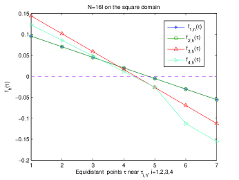
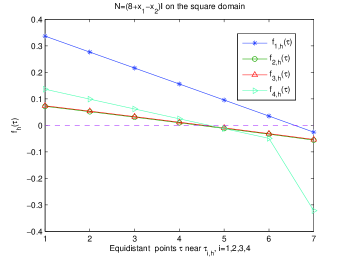
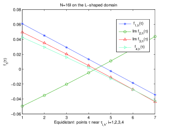
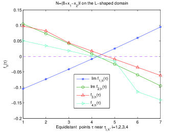
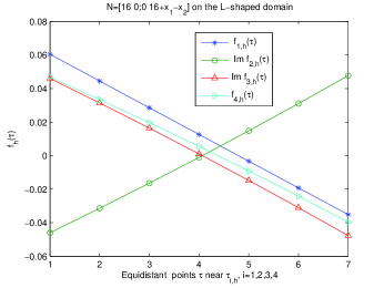
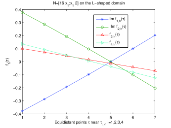
Figure 1: $f_{h}(\tau)$ computed by the second family of curl-curl element ($l=3$).

Table 1: Numerical eigenvalues by the second family of curl-curl element ($l=3$) on the unit square with $h_{0}=\frac{\sqrt{2}}{8}$.

$N=16I$					$N=(8+x_{1}-x_{2})I$
$j$	$h$	$k_{j,h}$	$r_{h}$	$|f^{\prime}_{h}(\tau_{j,h})|$	$k_{j,h}$	$r_{h}$	$|f^{\prime}_{h}(\tau_{j,h})|$
1	$h_{0}$	1.927882001		0.65	3.385891713		0.80
1	$\frac{h_{0}}{2}$	1.927871544	5.14	0.65	3.385803303	5.92	0.80
1	$\frac{h_{0}}{4}$	1.927871248		0.65	3.385801845		0.80
2	$h_{0}$	1.927882001		0.65	3.505047783		0.31
2	$\frac{h_{0}}{2}$	1.927871544	5.14	0.65	3.504614745	5.51	0.31
2	$\frac{h_{0}}{4}$	1.927871248		0.65	3.504605216		0.31
3	$h_{0}$	2.333811701		0.92	3.505832045		0.31
3	$\frac{h_{0}}{2}$	2.333763623	5.78	0.92	3.505632716	4.82	0.31
3	$\frac{h_{0}}{4}$	2.333762748		0.92	3.505625649		0.31
4	$h_{0}$	2.343100969		0.79	3.616924954		0.51
4	$\frac{h_{0}}{2}$	2.343034872	5.75	0.79	3.616668920	5.37	0.51
4	$\frac{h_{0}}{4}$	2.343033643		0.79	3.616662744		0.51

Table 2: Numerical eigenvalues by the second family of curl-curl element ($l=3$) on the L-shaped domain with $h_{0}=\frac{\sqrt{2}}{4}$.

$N=16I$					$N=(8+x_{1}-x_{2})I$
$j$	$h$	$k_{j,h}$	$r_{h}$	$|f^{\prime}_{h}(\tau_{j,h})|$	$j$	$h$	$k_{j,h}$	$r_{h}$	$|f^{\prime}_{h}(\tau_{j,h})|$
1	$h_{0}$	1.17856958		0.67	1,2	$h_{0}$	1.2921312		1.90
1	$\frac{h_{0}}{2}$	1.1783712	1.50	0.67			$\pm$0.6797234i
1	$\frac{h_{0}}{4}$	1.1783009		0.67	1,2	$\frac{h_{0}}{2}$	1.2925357	1.31	1.89
3,4	$h_{0}$	1.2025191		0.96			$\pm$0.6797410i
		$\pm$0.4412079i			1,2	$\frac{h_{0}}{4}$	1.2926992		1.89
3,4	$\frac{h_{0}}{2}$	1.2030798	1.41	0.96			$\pm$0.6797388i
		$\pm$0.4411595i			3	$h_{0}$	2.0370694		0.65
3,4	$\frac{h_{0}}{4}$	1.2032896		0.96	3	$\frac{h_{0}}{2}$	2.0365801	2.35	0.65
		$\pm$0.4411257i			3	$\frac{h_{0}}{4}$	2.0364839		0.65
2	$h_{0}$	1.2717694		0.56	4	$h_{0}$	2.0630459		0.40
2	$\frac{h_{0}}{2}$	1.2713493	1.76	0.56	4	$\frac{h_{0}}{4}$	2.0608619	1.42	0.40
2	$\frac{h_{0}}{4}$	1.2712256		0.56	4	$\frac{h_{0}}{4}$	2.0600483		0.40

Table 3: Numerical eigenvalues by the second family of curl-curl element ($l=3$) on the L-shaped-domain with $h_{0}=\frac{\sqrt{2}}{4}$.

$N=[16~{}0;0~{}16+x_{1}-x_{2}]$					$N=[16~{}x_{1};x_{1}~{}2]$
$j$	$h$	$k_{j,h}$	$r_{h}$	$|f^{\prime}_{h}(\tau_{j,h})|$	$j$	$h$	$k_{j,h}$	$r_{h}$	$|f^{\prime}_{h}(\tau_{j,h})|$
1	$h_{0}$	1.188137		0.67	1,2	$h_{0}$	1.5794070		4.67
1	$\frac{h_{0}}{2}$	1.187914	1.47	0.67			$\pm$1.0033762i
1	$\frac{h_{0}}{4}$	1.187833		0.67	1,2	$\frac{h_{0}}{2}$	1.5799704	0.89	4.67
2,3	$h_{0}$	1.2000971		0.97			$\pm$1.0032588i
		$\pm$0.4413211i			1,2	$\frac{h_{0}}{4}$	1.5802770		4.67
2,3	$\frac{h_{0}}{2}$	1.2006542	1.40	0.96			$\pm$1.0032045i
		$\pm$0.4412676i			3	$h_{0}$	2.1671018		0.65
2,3	$\frac{h_{0}}{4}$	1.2008635		0.96	3	$\frac{h_{0}}{2}$	2.1654994	2.08	0.65
		$\pm$0.4412319i			3	$\frac{h_{0}}{4}$	2.1651206		0.65
4	$h_{0}$	1.2842037		0.57	4	$h_{0}$	2.5257509		0.86
4	$\frac{h_{0}}{2}$	1.2837800	1.77	0.57	4	$\frac{h_{0}}{2}$	2.5214581	2.09	0.86
4	$\frac{h_{0}}{4}$	1.2836553		0.57	4	$\frac{h_{0}}{4}$	2.5204517		0.86

Table 4: The numerical eigenvalues by lowest order element on the unit square with $h_{0}=\frac{\sqrt{2}}{16}$.

$N=16I$					$N=(8+x_{1}-x_{2})I$
$j$	$h$	$k_{j,h}$	$r_{h}$	$|f^{\prime}_{h}(\tau_{j,h})|$	$k_{j,h}$	$r_{h}$	$|f^{\prime}_{h}(\tau_{j,h})|$
1	$h_{0}$	1.9556		0.64	3.4855		0.77
1	$\frac{h_{0}}{2}$	1.9348	2.00	0.65	3.4116	1.94	0.79
1	$\frac{h_{0}}{4}$	1.9296	2.00	0.65	3.3923	1.98	0.80
1	$\frac{h_{0}}{8}$	1.9283		0.65	3.3874		0.80
2	$h_{0}$	1.9773		0.62	3.6570		0.32
2	$\frac{h_{0}}{2}$	1.9400	2.04	0.65	3.5430	2.02	0.31
2	$\frac{h_{0}}{4}$	1.9309	1.98	0.65	3.5149	2.01	0.31
2	$\frac{h_{0}}{8}$	1.9286		0.65	3.5079		0.31
3	$h_{0}$	2.3787		0.86	3.8035		0.39
3	$\frac{h_{0}}{2}$	2.3465	1.81	0.89	3.5885	1.76	0.31
3	$\frac{h_{0}}{4}$	2.3373	1.82	0.91	3.5252	2.03	0.31
3	$\frac{h_{0}}{8}$	2.3347		0.92	3.5097		0.31
4	$h_{0}$	2.4270		0.80	3.8496		0.45
4	$\frac{h_{0}}{2}$	2.3624	2.12	0.80	3.6598	2.54	0.50
4	$\frac{h_{0}}{4}$	2.3475	2.13	0.79	3.6272	2.04	0.51
4	$\frac{h_{0}}{8}$	2.3441		0.79	3.6193		0.51

Table 5: The numerical eigenvalues by lowest order element on the L-shaped domain with $h_{0}=\frac{\sqrt{2}}{16}$.

$N=16I$					$N=(8+x_{1}-x_{2})I$
$j$	$h$	$k_{j,h}$	$r_{h}$	$|f^{\prime}_{h}(\tau_{j,h})|$	$j$	$h$	$k_{j,h}$	$r_{h}$	$|f^{\prime}_{h}(\tau_{j,h})|$
1	$h_{0}$	1.1887		0.66	1,2	$h_{0}$	1.2911		1.91
1	$\frac{h_{0}}{2}$	1.1810	1.94	0.67			$\pm$0.6823i
1	$\frac{h_{0}}{4}$	1.1790	1.86	0.67	1,2	$\frac{h_{0}}{2}$	1.2919	1.54	1.90
1	$\frac{h_{0}}{8}$	1.1784		0.67			$\pm$0.6804i
3,4	$h_{0}$	1.1992		0.97	1,2	$\frac{h_{0}}{4}$	1.2924	1.41	1.90
		$\pm$0.4436i					$\pm$0.6799i
3,4	$\frac{h_{0}}{2}$	1.2018	1.50	0.97	1,2	$\frac{h_{0}}{8}$	1.2926		1.89
		$\pm$0.4418i					$\pm$0.6798i
3,4	$\frac{h_{0}}{4}$	1.2028	1.48	0.97	3	$h_{0}$	2.0675		0.63
		$\pm$0.4413i			3	$\frac{h_{0}}{2}$	2.0443	2.00	0.64
3,4	$\frac{h_{0}}{8}$	1.2032		0.96	3	$\frac{h_{0}}{4}$	2.0385	1.93	0.64
		$\pm$0.4412i			3	$\frac{h_{0}}{8}$	2.0370		0.65
2	$h_{0}$	1.2880		0.57	4	$h_{0}$	2.1037		0.40
2	$\frac{h_{0}}{2}$	1.2757	1.90	0.56	4	$\frac{h_{0}}{2}$	2.0716	1.90	0.40
2	$\frac{h_{0}}{4}$	1.2724	1.89	0.56	4	$\frac{h_{0}}{4}$	2.0630	1.82	0.40
2	$\frac{h_{0}}{8}$	1.2715		0.56	4	$\frac{h_{0}}{8}$	2.0606		0.40

Table 6: The numerical eigenvalues by lowest order element on the L-shaped-domain with $h_{0}=\frac{\sqrt{2}}{16}$.

$N=[16~{}0;0~{}16+x_{1}-x_{2}]$					$N=[16~{}x_{1};x_{1}~{}2]$
$j$	$h$	$k_{j,h}$	$r_{h}$	$|f^{\prime}_{h}(\tau_{j,h})|$	$j$	$h$	$k_{j,h}$	$r_{h}$	$|f^{\prime}_{h}(\tau_{j,h})|$
1	$h_{0}$	1.1984		0.66	1,2	$h_{0}$	1.5803		4.69
1	$\frac{h_{0}}{2}$	1.1906	1.89	0.67			$\pm$1.007i
1	$\frac{h_{0}}{4}$	1.1885	2.02	0.67	1,2	$\frac{h_{0}}{2}$	1.5798	1.83	4.67
1	$\frac{h_{0}}{8}$	1.1880		0.67			$\pm$1.004i
2,3	$h_{0}$	1.1968		0.97	1,2	$\frac{h_{0}}{4}$	1.5801	1.59	4.67
		$\pm$0.4438i					$\pm$1.004i
2,3	$\frac{h_{0}}{2}$	1.1994	1.44	0.96	1,2	$\frac{h_{0}}{8}$	1.5803		4.67
		$\pm$0.4420i					$\pm$1.003i
2,3	$\frac{h_{0}}{4}$	1.2004	1.65	0.96	3	$h_{0}$	2.2286	1.98	0.65
		$\pm$0.4414i			3	$\frac{h_{0}}{2}$	2.1812		0.65
2,3	$\frac{h_{0}}{8}$	1.2008		0.96	3	$\frac{h_{0}}{4}$	2.1692	1.95	0.65
		$\pm$0.4413i			3	$\frac{h_{0}}{8}$	2.1661		0.65
4	$h_{0}$	1.3006		0.57	4	$h_{0}$	2.6139		0.83
4	$\frac{h_{0}}{2}$	1.2881	1.92	0.57	4	$\frac{h_{0}}{2}$	2.5446	1.94	0.85
4	$\frac{h_{0}}{4}$	1.2848	1.95	0.57	4	$\frac{h_{0}}{4}$	2.5266	1.91	0.86
4	$\frac{h_{0}}{8}$	1.2839		0.57	4	$\frac{h_{0}}{8}$	2.5218		0.86

Acknowledgements.   This work was partially supported by supported by the National Natural Science Foundation of China (Grants. 12001130, 11871092, NSAF 1930402), China Postdoctoral Science Foundation (no. 2020M680316), and Science and Technology Foundation of Guizhou Province (no. ZK[2021]012).

References

• (1) J. An and J. Shen. A spectral-element method for transmission eigenvalue problems. J. Sci. Comput., 57(2013), 670-688
• (2) J. An and Z. Zhang. An efficient spectral-Galerkin approximation and error analysis for Maxwell transmission eigenvalue problems in spherical geometries. J. Sci. Comput., 75(2018), 157-181.
• (3) I. Babuska, J. Osborn. Eigenvalue Problems, in: P .G. Ciarlet, J. L. Lions, (Ed.), Finite Element Methods (Part 1), Handbook of Numerical Analysis, vol.2, Elsevier Science Publishers, North-Holand, 1991, pp. 640-787.
• (4) S. C. Brenner, J. Sun, and L. Sung. Hodge decomposition methods for a quad-curl problem on planar domains. J. Sci. Comput., 73(2017), 495-513.
• (5) F. Brezzi and M. Fortin. Mixed and Hybrid Finite Element Methods, vol. 15, Springer, New York, NY, USA, 1991.
• (6) F. Cakoni, M. Cayoren, and D. Colton. Transmission eigenvalues and the nondestructive testing of dielectrics. Inverse Problems, 24(2008), 065016.
• (7) F. Cakoni, H. Haddar. On the existence of transmission eigenvalues in an inhomogenous medium, Appl. Anal., 88(2009), pp. 475-493.
• (8) F. Cakoni, D. Gintides, and H. Haddar. The existence of an infinite discrete set of transmission eigenvalues. SIAM J. Math. Anal., 42(2010), 237-255.
• (9) F. Cakoni, D. Coltionk P. Monk, and J. Sun. The inverse electromagnetic scattering problem for anisotropic media, Inverse Problems, 26(2010), 074004 (14pp).
• (10) F. Cakoni, P. Monk, and J. Sun. Error analysis for the finite element approximation of transmission eigenvalues, Comput. Methods Appl. Math., 14(2014), 419-427.
• (11) D. Colton, R. Kress, Inverse Acoustic and Electromagnetic Scattering Theory, 2nd ed., Vol. 93 in Applied Mathematical Sciences, Springer, New York, 1998.
• (12) D. Colton, P. Monk, and J. Sun. Analytical and computational methods for transmission eigenvalues. Inverse Problems, 26(2010), 045011
• (13) D. Colton, L. P$\ddot{a}$iv$\ddot{a}$rinta, and J. Sylvester. The interior transmission problem. Inverse Problem Imaging, 1(2007), 13-28.
• (14) F. Chatelin. Spectral Approximations of Linear Operators, Academic Press, New York, 1983.
• (15) R. Hiptmair. Finite elements in computational electromagnetism. Acta Numer., 11 (2002), 237-339.
• (16) Q. Hong, J. Hun, S. Shu, and J. Xu. A discontinuous galerkin method for the fourth-order curl problem. J. Comp. Math., 30(2012), 565-578.
• (17) K. Hu, Q. Zhang, and Z. Zhang. Simple curl-curl-conforming finite elements in two dimensions, SIAM Journal on Scientific Computing, 42(2020), A3859-A3877.
• (18) K. Hu, Q. Zhang, and Z. Zhang. A family of finite element stokes complexes in three dimensions. arXiv:2008.03793v1 [math.NA], Aug 2020.
• (19) T. M. Huang, W. Q. Huang, and W. W. Lin. A robust numerical algorithm for computing Maxwell’s transmission eigenvalue problems, SIAM J. Sci. Comput. 37(2015), A2403-A2423.
• (20) X. Ji, J. Sun, and H. Xie. A multigrid method for Helmholtz transmission eigenvalue problems. J. Sci. Comput., 60(2014), 276-294.
• (21) A. Kleefeld and L. Pieronek. The method of fundamental solutions for computing acoustic interior transmission eigenvalues. Inverse Problems, 34 (2018), 035007
• (22) F. Kikuchi. Weak formulations for finite element analysis of an electromagnetic eigenvalue problem. Scientific Papers of the College of Arts and Sciences, University of Tokyo, 38 (1988), 43-67.
• (23) F. Kikuchi. On a discrete compactness property for the Nedelec finite elements. J.fac.sci.univ.tokyo Sect. 1A Math, 36(1989), 479-490.
• (24) P. Monk. Finite Element Methods for Maxwell’s Equations, Oxford University Press, Oxford, UK, 2003.
• (25) P. Monk and J. Sun. Finite element methods for Maxwell’s tranmission eigenvalues. SIAM. J. Sci. Comput., 34(2012), B247-B264.
• (26) P. Monk and L. Demkowicz. Discrete compactness and the approximation of Maxwell’s equations in $\mathbb{R}^{3}$. Math. Comp., 70(2000), pp. 507-523.
• (27) J. C. N$\acute{e}$d$\acute{e}$lec. Mixed finite elements in $R^{3}$. Numer. Math., 35(1980), 315-341.
• (28) J. E. Osborn. Spectral approximation for compact operators. Math. Comput., 26(1975), 712-725.
• (29) L. Päivärinta and J. Sylvester. Transmission eigenvalues, SIAM J. Math. Anal., 40(2008), 738-753.
• (30) J. Sun. Iterative methods for transmission eigenvalues, SIAM J. Numer. Anal., 49(2011), pp. 1860-1874.
• (31) J. Sun and L. Xu. Computation of Maxwell’s transmission eigenvalues and its applications in inverse medium problems. Inverse Problems, 29 (2013), 104013 (18pp).
• (32) J. Sun. A mixed FEM for the quad-curl eigenvalue problem, Numer. Math., 132(2016), 185-200.
• (33) L. Wang, W. Shan, H. Li, and Z. Zhang. ${\bf H}(\mathrm{curl}^{2})$-conforming quadrilateral spectral element method for quad-curl problems. Math. Mod. Meth. Appl. Sci., 31(2021), 1951-1986.
• (34) H. Xie and X. Wu. A multilevel correction method for interior transmission eigenvalue problem, J. Sci. Comput. 72(2017), 586-604.
• (35) Y. Yang, J. Han, and H. Bi. Error estimates and a two grid scheme for approximating transmission eigenvalues. arXiv: 1506.06486 V2 [math. NA] 2 Mar 2016.
• (36) Y. Yang, H. Bi, H. Li, and J. Han. Mixed method for the helmholtz transmission eigenvalues. SIAM J. Sci. Comput., 38(2016), A1383-A1403.
• (37) Q. Zhang, L. Wang, and Z. Zhang. An $H(\mathrm{curl}^{2})$-conforming finite element in 2 dimensions and applications to the quad-curl problem. SIAM J. Sci. Comput., 41(2019), A1527-A1547.
• (38) S. Zhang. Mixed schemes for quad-curl equations, ESAIM: M2AN, 52 (2018), 147-161.
• (39) B. Zheng, B. Hu, and Q. Xu. A nonconforming element method for fourth order curl equations in $\mathbb{R}^{3}$. Math. Comput., 276(2011), 1871-1886.