Bayesian Predictive Decision Synthesis

Abstract

Decision-guided perspectives on model uncertainty expand traditional statistical thinking about managing, comparing and combining inferences from sets of models. Bayesian predictive decision synthesis (BPDS) advances conceptual and theoretical foundations, and defines new methodology that explicitly integrates decision-analytic outcomes into the evaluation, comparison and potential combination of candidate models. BPDS extends recent theoretical and practical advances based on both Bayesian predictive synthesis and empirical goal-focused model uncertainty analysis. This is enabled by the development of a novel subjective Bayesian perspective on model weighting in predictive decision settings. Illustrations come from applied contexts including optimal design for regression prediction and sequential time series forecasting for financial portfolio decisions.

Keywords: Bayesian decision analysis, Decision-guided model weighting, Generalised Bayesian updating, Entropic tilting, Model uncertainty, Optimal design, Portfolio decisions

Introduction

Questions of model assessment, calibration, comparison and combination define continuing conceptual and practical challenges to all areas of quantitative modelling. Recent developments in Bayesian thinking has generated new methodology motivated by a range of challenging applications  (e.g. Billio et al., 2013; Amisano and Geweke, 2017; Kapetanios et al., 2015; Aastveit et al., 2019; McAlinn and West, 2019; West, 2020; Vannitsem et al., 2021; Aastveit et al., 2023). However, while advancing methodology for improved prediction, such research developments have also raised foundational questions on the scope of model uncertainty analysis more broadly.

A key theme is recognising explicit inferential goals to reflect the intended uses of models when addressing model assessment and uncertainty. This perspective is increasingly recognised (e.g. Clyde and Iversen, 2013; McAlinn and West, 2019; McAlinn et al., 2020, and references therein), with numerous applied studies emphasising the relevance of differentially weighting models modulo specified goals (e.g. Geweke and Amisano, 2011, 2012; Nakajima and West, 2013; Kapetanios et al., 2015; West, 2020; McAlinn, 2021). This theme has been recently highlighted in Lavine et al. (2021) and Loaiza-Maya et al. (2021). These authors use explicit model weightings based on so-called “Gibbs probabilities”that incorporate metrics related to utility (or “score”) functions evaluating predictions of specific, defined outcomes. Studies there highlight the relevance of this perspective, and its dominance over traditional “goal neutral”statistical approaches such as Bayesian model averaging when explicit goals can be defined and used to focus and guide the analysis.

This paper contributes to this area by addressing foundational perspectives on model comparison and combination that reflect both predictive and decision goals. The perspective follows Lindley (1992) in emphasising both the inferential “Yin”and the decision analytic “Yang”of Bayesian analysis. Developments build on the foundation of Bayesian predictive synthesis (BPS: McAlinn et al., 2018; McAlinn and West, 2019; Johnson and West, 2022). Recent methodological developments linked to the BPS foundations are increasingly impacting forecasting and related applications, especially in economics and finance (e.g. Bassetti et al., 2018; McAlinn et al., 2020; Aastveit et al., 2019; McAlinn, 2021; Aastveit et al., 2023). A stylised class of BPS mixture models– referred to as mixture-BPS– is extended to integrate explicit decision goals and outcomes into the model uncertainty framework. Modelling choices and implementation exploit entropic tilting (ET), originally introduced in predictive analyses to condition predictive distributions on sets of externally-imposed constraints (Robertson et al., 2005; Krüger et al., 2017; West, 2023). As developed here, ET defines a broader decision analysis setting for exploring, contrasting and integrating constraints into predictive inferences, with opportunities for exploitation in new ways. Key foundational connections are made with generalised belief updating, in which data-based evidence is represented in likelihood functions constructed based on defined loss or utility functions (Jiang and Tanner, 2008; Bissiri et al., 2016; Bernaciak and Griffin, 2022) This links to integrating decision-analysis perspectives into Bayesian updating under model misspecification (e.g. Zhang, 2006a, b; Jiang and Tanner, 2008; Watson and Holmes, 2016). These theoretical themes tie into Bayesian model scoring based on Gibbs model probabilities (Lavine et al., 2021; Loaiza-Maya et al., 2021) that explicitly focus on incorporating specific predictive goals into the model evaluation processes.

Integration of ET with BPS defines the new framework of Bayesian predictive decision synthesis (BPDS). This recognises that formal decision analysis will often yield differences across models in the implied optimal decisions and realised utilities, so a primary focus on decisions and their outcomes is relevant in model comparison and combination. Integration with other recent developments in decision-guided model scoring and weighting, including adaptive variable selection (Lavine et al., 2021), enables the incorporation of information on historical predictions and decision outcomes in the overall BPDS framework. This is especially relevant in development in sequential time series applications with dynamic models for forecasting and decisions.

Section 2 reviews aspects of the foundations and nature of mixture-BPS that is of central interest here. This is presented in the traditional predictive setting with no links to decision analysis. Section 3 discusses new, stylised versions of mixture-BPS models, and discusses theoretical foundations in both entropic tilting and generalised Bayesian updating. These new developments are again presented in the purely predictive setting, not addressing decisions. The extensions to integrate model-specific decisions, defining the new BPDS framework, are presented in Section 4. Detailed developments are made in two example settings. Section 5 concerns optimal design variable selection in a simple regression setting as an illuminating, idea-fixing example. Section 6 develops an extensive example in sequential portfolio decision analysis in time series. Concluding comments are in Section 7.

Bayesian Predictive Synthesis (BPS) and Mixture Models

Traditional Model Uncertainty Framework

Begin with the usual model uncertainty framework of a discrete mixture of distributions for outcomes of interest. The quantities of interest and notation are as follows.

• An outcome $q-$vector $\mathbf{y}$ in sample space ${\mathcal{Y}}$. Examples are the returns on $m$ equities at the next time period in a financial time series forecasting application or the outcome in a response surface design study.

• A set of $J$ models ${\mathcal{M}}_{j}$, $j=1{:}J,$ such as a set of dynamic regression models for the return vector with different predictors across models, or other distinct model forms.

• Model ${\mathcal{M}}_{j}$ defines a predictive density function $p_{j}(\mathbf{y}|{\mathcal{M}}_{j})$, the set of which is denoted by ${\mathcal{P}}=\{p_{1}(\mathbf{y}|{\mathcal{M}}_{1}),\ldots,p_{J}(\mathbf{y}|{\mathcal{M}}_{J})\}.$

• Model probabilities $\pi_{j}=Pr({\mathcal{M}}_{j})$, such as from traditional Bayesian model averaging based on past data and information denoted by ${\mathcal{D}}.$

• The dependence of models and model probabilities on ${\mathcal{D}}$ is not made explicit in the notation, for clarity; such dependence is, of course, critical in applications and implicit throughout.

The predictive mixture $p(\mathbf{y})=\sum_{j=1{:}J}\pi_{j}p_{j}(\mathbf{y}|{\mathcal{M}}_{j})$ is implied under traditional Bayesian model averaging (BMA). A well-known concern with BMA is that it does not address model set incompleteness, i.e., that all models ${\mathcal{M}}_{j}$ may be poor predictors (as well as all “wrong”), a key point that is revisited below in discussing BPS.

Bayesian Predictive Synthesis: Mixture-BPS

Background and Mixture-BPS Model Form

Bayesian predictive synthesis (BPS) adopts a subjective Bayesian view of model uncertainty in which the set of predictive densities ${\mathcal{P}}$ is regarded by a Bayesian modeller as information to condition upon in forming their predictions. This is known as the “supra-Bayesian” perspective (Lindley et al., 1979), and provides opportunities to adjust model-specific predictions for biases and miscalibration, and to at least partly address model set incompleteness. BPS evolved from the theory of agent opinion analysis (West and Crosse, 1992; West, 1992) which built on foundations in Genest and Schervish (1985). The approach is semi-parametric Bayesian, and results in identifying a subclass of predictive distributions that are consistent with the modeller’s partial specification of prior uncertainty about $\mathbf{y}$ and ${\mathcal{P}}.$ Johnson and West (2022), and McAlinn and West (2019), discuss the foundational theory, and present a range of examples among which outcome dependent mixture-BPS represents the special case of focus here. This subclass of BPS models is the foundation for the decision-focused extensions in Section 4 below. In one specific subset of mixture-BPS models, the modeller’s predictive distribution– conditional on learning ${\mathcal{P}}$– has the form

$$f(\mathbf{y}|{\mathcal{P}})\propto\sum_{j=0{:}J}\pi_{j}\alpha_{j}(\mathbf{y})p_{j}(\mathbf{y}|{\mathcal{M}}_{j})$$ (1)

where (i) $\pi_{0{:}J}$ is a set of initial model probabilities; (ii) $p_{0}(\mathbf{y}|{\mathcal{M}}_{0})$ is the density of a baseline distribution specified by the modeller and based on a notional baseline model ${\mathcal{M}}_{0}$; and (iii) $\alpha_{j}(\cdot)$, $(j=0{:}J),$ are non-negative weight functions.

Eqn. (1) can be rewritten as

$$f(\mathbf{y}|{\mathcal{P}})=\sum_{j=0{:}J}\tilde{\pi}_{j}f_{j}(\mathbf{y}|{\mathcal{M}}_{j})\ \ \textrm{where}\ \ f_{j}(\mathbf{y}|{\mathcal{M}}_{j})=\alpha_{j}(\mathbf{y})p_{j}(\mathbf{y}|{\mathcal{M}}_{j})/a_{j},\,\,j=0{:}J,$$ (2)

in which

$$a_{j}=\int_{\mathbf{y}}\alpha_{j}(\mathbf{y})p_{j}(\mathbf{y}|{\mathcal{M}}_{j})d\mathbf{y}\ \ \textrm{and}\ \ \tilde{\pi}_{j}=k\pi_{j}a_{j}\ \ \textrm{with}\ \ k^{-1}=\sum_{j=0{:}J}\pi_{j}a_{j}.$$

Before discussing the details of these ingredients and their implications, the constructive use of the above theoretical result is emphasised. That is, models of the form of eqn. (2) can be explored for various choices of the weight functions $\alpha_{j}(\mathbf{y});$ choosing these directly defines the predictive $f(\mathbf{y}|{\mathcal{P}})$. The current paper adopts this perspective. Note also that, in applications in sequential time series forecasting, each of the $\mathbf{y},\pi_{j},\alpha_{j}(\cdot),{\mathcal{P}}$ and of course ${\mathcal{D}}$ become time-indexed; see examples in Johnson and West (2022). Our time series example in Section 6 follows this path.

Mixture-BPS Weight Functions

The $\alpha_{j}(\mathbf{y})$ terms explicitly depend on the future outcome $\mathbf{y}$, and can be exploited to address anticipated biases and lack of calibration in each ${\mathcal{M}}_{j}$, as well as to increase/decrease weight on any model in different regions of the outcome space of $\mathbf{y}.$ For example, a specific model ${\mathcal{M}}_{i}$ may be expected to predict relatively more accurately in regions where element $y_{1}$ is high, but poorly when $y_{1}$ is low. This relates to considerations of relative areas of “expertise” across the model set. Appropriately chosen weight (or “kernel”) functions $\alpha_{j}(\cdot)$ will then change the contributions of the ${\mathcal{M}}_{j}$ to $f(\mathbf{y}|{\mathcal{P}})$ accordingly as they modify the $p_{j}(\mathbf{y}|{\mathcal{M}}_{j})$ to resulting $f_{j}(\mathbf{y}|{\mathcal{M}}_{j})$ densities. Correspondingly, the $\tilde{\pi}_{j}$ are modified model probabilities, adjusting the initial $\pi_{j}$ based on concordance of $\alpha_{j}(\mathbf{y})$ with $p_{j}(\mathbf{y}|{\mathcal{M}}_{j})$. The consideration of outcome-dependent calibration led to important early work using forms similar to eqn. (2) in empirical studies in macroeconomic forecasting, beginning with Kapetanios et al. (2015). Mixture-BPS underpins such developments and extends such approaches to admit a possible baseline model indexed by $j=0$ as well as specified initial model probabilities $\pi_{j}$ based on historical data and information ${\mathcal{D}}.$

Baseline Distribution

The baseline distribution is an important feature; it explicitly admits and addresses the potential that “all models are wrong”. That is, the question of model set incompleteness (McAlinn et al., 2018; Aastveit et al., 2019; McAlinn et al., 2020; Giannone et al., 2021), earlier and often referred to as the “model space open”– or $``{\mathcal{M}}-$open”– setting (Bernardo and Smith, 1994; West and Harrison, 1997, section 12.2;  Clyde and George, 2004; Clyde and Iversen, 2013). It is often important to adopt this view, admitting that predictions based on any of the candidate models may be poor, and assign some non-zero probability on a “safe-haven” or fall-back predictive; see also DeGroot (1980) for a pertinent historical perspective. $p_{0}(\cdot|{\mathcal{M}}_{0})$ may be chosen, for example, as an over-dispersed density, putting higher mass on regions of $\mathbf{y}$ likely to be less well-supported under any of the ${\mathcal{M}}_{j}.$ Such a baseline will receive increasing weight as outcome $\mathbf{y}$ predictions from the model set of $J$ models are more and more inaccurate. Thus larger values of $\tilde{\pi}_{0}$ will indicate that ${\mathcal{M}}_{j}$ models for $j=1{:}J$ are collectively performing poorly. The conceptual and technical relationships with the construction of baseline “alternative models” in Bayesian analysis in other areas is to be noted (West, 1986; West and Harrison, 1997, section 11.4).

Initial Model Weights

The $\pi_{j}$ can be regarded as initial model weights based on historical data and prior information ${\mathcal{D}}$ that the modeller deems relevant to forecasting $\mathbf{y}.$ In a sequential time series context, for example, they may be discounted versions of past BMA weights, as used, for example in  Zhao et al. (2016) and adaptive variable selection (AVS) in Lavine et al. (2021). More generally, the modeller has the flexibility to choose the initial weights as a separate consideration to that of specifying the $\alpha_{j}(\cdot)$ weight functions which address questions of anticipated model bias and relative areas of expertise.

Example: BMA as a Special Case

Based on the initial model probabilities $\pi_{1{:}J},$ it is immediate that BPS specialises to BMA with the choices $\pi_{0}=0$ and $\alpha_{j}(\mathbf{z}_{j})=1$ for $j=1{:}J$. Obviously, there is no future outcome dependency here and the input predictives $p_{j}(\mathbf{y}|{\mathcal{M}}_{j})$ are not modified prior to averaging.

BMA does not recognise model set incompleteness. However, this simple mixture-BPS example with a non-zero $\pi_{0}$ opens a path to potentially raise awareness of, and adapt to, the lack of predictive ability of the set of models. Such a minor extension of BMA does, of course, require an appropriately chosen $p_{0}(\cdot|{\mathcal{M}}_{0})$.

Examples: AVS and Goal-Focused Scoring of Historical Predictions

Important special cases– again with no outcome dependence– link mixture weights to historical data and past outcomes in the predictive performance of each model. Scoring models modulo specified forecasting goals has been stressed in various ways (e.g. Geweke and Amisano, 2011, 2012; Nakajima and West, 2013; Kapetanios et al., 2015; West, 2020; McAlinn, 2021), and recently highlighted in AVS (Lavine et al., 2021) and targeted prediction (Loaiza-Maya et al., 2021).

Recall that ${\mathcal{D}}$ denotes all prior information the modeller deems relevant to combining forecast information for $\mathbf{y},$ recognizing that the initial model probabilities $\pi_{j}$ are inherently dependent on ${\mathcal{D}}.$ In a sequential time series context, and in which models are distinguished based on chosen sets of covariates in a dynamic linear modelling framework, the AVS approach of Lavine et al. (2021) uses scores that reflect past predictive accuracy on outcomes of applied interest. The term adaptive variable selection explicitly relates to the models being based on different sets of covariates, and the changes over time in chosen covariates in a sequential time series setting. Examples of scores include predictions of multi-step ahead outcomes in the time series, and multi-step paths over several time periods ahead. Ignoring the time indexing for a sequential time series setting, AVS uses outcome-independent choices $\pi_{0}=0$ and $\alpha_{j}(\mathbf{y})\equiv\alpha_{j}\propto\exp\{\tau s_{j}({\mathcal{D}})\}$ for $j=1{:}J,$ not depending on $\mathbf{y}.$ Here $\tau$ is a chosen scale factor and $s_{j}({\mathcal{D}})$ is a chosen univariate score for model ${\mathcal{M}}_{j}$ based on historical information ${\mathcal{D}}.$ This is a special case of mixture-BPS with dynamic extension for the time series setting. Then, note that the approach in Loaiza-Maya et al. (2021) adopts a functional form of weights similar to those defining AVS.

Entropic Tilting and Generalised Bayes

Exponential Score Weight Functions

Adopt models in which the BPS weight functions are defined by

$$\alpha_{j}(\mathbf{y})=\exp\{{\bm{\tau}}^{\prime}\mathbf{s}_{j}(\mathbf{y})\},\,\,j=0{:}J,$$ (3)

where each $\mathbf{s}_{j}(\mathbf{y})$ is a $k-$vector of prescribed scores that depend on the future outcome $\mathbf{y}$. The scores are chosen to reflect utilities, so that higher scores are desirable. The use of a vector score allows consideration of multiple aspects of model evaluation, i.e., multi-attribute utilities. The $k-$vector ${\bm{\tau}}$ defines relative weights and directional relevance of the elements of the score vector, so that the ${\mathcal{M}}_{j}$ are relatively weighted according to the resulting aggregate score.

The exponential, weighted-score form of $\alpha_{j}(\mathbf{y})$ is underpinned by theoretical foundations presented in Sections 3.2 and 3.3 below. It also parallels and extends score-based methods that use historical outcomes to define weight functions via so-called “Gibbs model probabilities”in generalised Bayesian updating, AVS and allied approaches (Bissiri et al., 2016; Lavine et al., 2021; Loaiza-Maya et al., 2021, and references therein). Key innovations here are that model weights in eqn. (3) depend on (i) the as yet unobserved outcome $\mathbf{y}$, and (ii) multiple predictive metrics in the vector score. This underlies the extension to integrate decision outcomes in Section 4 below. Prior to that development, the underlying foundational theory is summarised.

Entropic and/or Exponential Tilting

Using eqn. (3), the BPS predictive densities $f_{j}(\cdot)$ in eqn. (2) are “exponentially tilted”modifications of the $p_{j}(\cdot|\cdot),$ i.e., $f_{j}(\mathbf{y}|{\mathcal{M}}_{j})\propto\exp\{{\bm{\tau}}^{\prime}\mathbf{s}_{j}(\mathbf{y})\}p_{j}(\mathbf{y}|{\mathcal{M}}_{j}).$ Exponential/entropic tilting (Robertson et al., 2005; Krüger et al., 2017; West, 2023) provides conceptual and theoretical foundation for this choice of the $\alpha_{j}(\cdot)$ as well as a constructive approach specifying the ${\bm{\tau}}$ vector.

First, recognise that the initial mixture model is fundamentally a joint distribution over outcomes and models together, i.e. the joint density/mass function $p(\mathbf{y},{\mathcal{M}}_{j})=p({\mathcal{M}}_{j})p(\mathbf{y}|{\mathcal{M}}_{j})=\pi_{j}p_{j}(\mathbf{y}|{\mathcal{M}}_{j})$ over $\mathbf{y}\in{\mathcal{Y}},j=1{:}J.$ Extend this to include a baseline case $j=0$ defined by the modeller. Then, for score vectors $\mathbf{s}_{j}(\mathbf{y})$ of chosen functional forms in $\mathbf{y}$, this extended mixture implies the initial expected score $\mathbf{m}_{\mathbf{0}}=E_{p}[\mathbf{s}_{j}(\mathbf{y})]=\sum_{j=0{:}J}\pi_{j}\mathbf{m}_{j,\mathbf{0}}$ where $\mathbf{m}_{j,\mathbf{0}}=\int_{\mathbf{y}}\mathbf{s}_{j}(\mathbf{y})p_{j}(\mathbf{y}|{\mathcal{M}}_{j})d\mathbf{y}$ is the expected score under $p_{j}(\cdot|{\mathcal{M}}_{j}).$ Since the score is a vector of utilities, $\mathbf{m}_{\mathbf{0}}$ represents a vector of benchmark expected utilities– benchmark as they are based on the initial distribution over $(\mathbf{y},{\mathcal{M}}_{j})$.

Entropic tilting (ET) investigates modifications of this joint distribution that are consistent with different expected scores. The relevant thinking here is that of improving, i.e., increasing scores relative to the initial mixture. Choose a $k-$vector $\mathbf{m}$ to define a target expected score; for example, elements of $\mathbf{m}$ may represent small % increases in expected score relative to $\mathbf{m}_{\mathbf{0}}.$ Predictive distributions over $(\mathbf{y},{\mathcal{M}}_{j})$ that have this or higher expected scores are then of interest– simply as they may result in increased realised scores. Exploring small/modest increases in expected scores relative to $\mathbf{m}_{\mathbf{0}}$ reflects a perspective that, while the initial mixture has been defined based on analysis to date– including past decision outcomes as well as predictions– it still represents a specific, chosen model, and small perturbations of it may yield improved predictions and decisions. It is important that chosen score functions be interpretable, so that the numerical values of elements of expected scores can be understood to aid specification of $\mathbf{m}.$ As noted above, in many cases this will be naturally assessed using percent changes over the expected score under the initial mixture. Further discussion in context is given in the design and portfolio examples below.

In its original form, ET operationalises these ideas by considering all distributions $f(\mathbf{y},{\mathcal{M}}_{j})$ under which $E_{f}[\mathbf{s}_{j}(\mathbf{y})]=\mathbf{m}$; then, among such distributions, ET identifies $f(\cdot,\cdot)$ that is Küllback-Leibler (KL) closest to $p(\cdot,\cdot).$ The natural KL direction is used: the divergence is that of $p(\cdot,\cdot)$ from $f(\cdot),$ i.e., $KL(f{||}p)=E_{f}[\log\{f(\mathbf{y},{\mathcal{M}}_{j})/p(\mathbf{y},{\mathcal{M}}_{j})\}]$ where the expectation is with respect to $f(\mathbf{y},{\mathcal{M}}_{j}).$ While this does not, a priori, impose any other assumptions on the form of $f(\mathbf{y},{\mathcal{M}}_{j}),$ the resulting the optimisation theoretically yields the unique solution $\tilde{\pi}_{j}f_{j}(\mathbf{y}|{\mathcal{M}}_{j})\propto\pi_{j}\alpha_{j}(\mathbf{y})p_{j}(\mathbf{y}|{\mathcal{M}}_{j})$ where $\alpha_{j}(\mathbf{y})$ has precisely the exponentially tilted form of eqn. (3). The unique optimising vector ${\bm{\tau}}$ depends on $\mathbf{m}$ and is implicitly defined so that the resulting BPS distribution $\tilde{\pi}_{j}f_{j}(\mathbf{y}|{\mathcal{M}}_{j})$ over $(\mathbf{y},{\mathcal{M}}_{j})$ has this expected score. Generally, there is a one-one correspondence between $\mathbf{m}$ and ${\bm{\tau}}$ emerging from convexity properties of exponential families (see, for example, the supplementary material in Tallman and West, 2022).

In addition to this theoretical foundation for the choice of weighting functions of eqn. (3), ET is constructive. It allows for calibration of mixture-BPS by defining the vector ${\bm{\tau}}$ consistent with a chosen target score $\mathbf{m}.$ Assuming the elements of the score vector are on contextually interpretable scales, specifying $\mathbf{m}$ is natural. Then, evidently the terms $a_{j}$ and hence $k$ in eqn. (2) depend on ${\bm{\tau}}$, and the resulting implicit equation to solve for ${\bm{\tau}}$ reduces to

$$\mathbf{m}=k\sum_{j=0{:}J}\pi_{j}\frac{\partial a_{j}}{\partial{\bm{\tau}}}.$$ (4)

This is often amenable to an easy numerical solution to compute ${\bm{\tau}}$ for a given $\mathbf{m}.$ It is also useful in reverse– to evaluate expected scores for any given values of ${\bm{\tau}}$.

ET has a broader, “relaxed” optimality property. Take target score $\mathbf{m}\geq\mathbf{m}_{\mathbf{0}}$ where the inequality is strict in at least one element of the vector. Then the ET optimal ${\bm{\tau}}$ ensuring expected score $\mathbf{m}$ does, in fact, minimise the KL divergence over all possible target scores $\mathbf{m}_{\ast}\geq\mathbf{m}$. This, and more detailed background and theoretical developments of entropic tilting, is shown in the supplementary manuscript of Tallman and West (2022). This supplement details the theory of ET for conditioning predictive distributions on constraints, includes new results related to connections with exponential families, elaborates on the “relaxed ET” (RET) extension, and includes examples of relevance more broadly and beyond the use in this paper.

Generalised Bayesian Updating and Approximate Models

A complementary theoretical foundation for the score form of BPS synthesis functions in eqn. (3) comes from generalised and robust Bayesian updating, earlier referenced (e.g. Bissiri et al., 2016, and others). In particular, there are intimate connections with the theme of Bayesian updating based on approximate models/priors as discussed in Watson and Holmes (2016). These authors work in terms of losses rather than utilities, and with only one loss metric; hence their results apply here with $\mathbf{s}_{j}(\mathbf{y})$ becoming scalar $s_{j}(\mathbf{y})$ and with $-s_{j}(\mathbf{y})$ representing their loss.

In a general setting, Watson and Holmes (2016) address uncertainty about a specified prior for a parameter or set of parameters. Mapping to the current setting, the “parameters” are $(\mathbf{y},{\mathcal{M}}_{j})$ and the baseline-extended initial model defines a specified prior $p(\mathbf{y},{\mathcal{M}}_{j})$ over $\mathbf{y}\in{\mathcal{Y}},j=0{:}J.$ Watson and Holmes (2016) ask questions about comparing other distributions $f(\cdot,\cdot)$ with $p(\cdot,\cdot)$ in terms of $KL(f{||}p)$ as used in ET above. A translation of the result discussed following Theorem 4.1 in their paper is key here. Consider all possible priors $f(\cdot,\cdot)$ in the Küllback-Leibler neighbourhood defined by $KL(f{||}p)\leq C$ for some chosen $C>0.$ That is, distributions $f(\cdot,\cdot)$ that are “close to” $p(\cdot,\cdot)$ in this KL sense with $C$ defining how close. Across this set of priors, find that $f(\cdot,\cdot)$ that maximises the implied expected utility (negative loss) $E_{f}[s_{j}(\mathbf{y})].$ The unique result is the exponentially tilted modification of the initial prior given by $f(\mathbf{y},{\mathcal{M}}_{j})\propto\pi_{j}\exp\{\tau_{C}s_{j}(\mathbf{y})\}p_{j}(\mathbf{y}|{\mathcal{M}}_{j}).$ Here $\tau_{C}\geq 0$ depends on $C$ and, as $C$ varies, is monotonically increasing in $C$.

This result is the theoretical dual of that based on ET, providing a complementary foundational perspective. The ET perspective has two distinctions, however. First, some of the interest in BPS, and decision-focused extensions below, lies in multiple utilities related to predictive and decision goals. The ET foundation admits multivariate scores and underlies the general result in eqn. (3). The dual generalised Bayesian updating result in Watson and Holmes (2016) concerned a univariate utility, with no obvious/easy theoretical multi-utility extension. The second point relates to interpretation in specification. With interpretable scores specified on understandable utility scales in an applied context, the ET approach is accessible in that a target score $\mathbf{m}$ can be related to the benchmark value(s) $\mathbf{m}_{\mathbf{0}}$ under the initial prior. In contrast, the specification of a practically relevant and interpretable $C$ to define a Küllback-Leibler neighbourhood in the complementary view is less natural and interpretable.

Local Perturbations of Expected Scores

Exploring target expected scores that are small/modest perturbations of those under the initial mixture is emphasised. With $\mathbf{m}_{\mathbf{0}}=E_{p}[\mathbf{s}_{j}(\mathbf{y})]$ implied under $p(\mathbf{y},{\mathcal{M}}_{j}),$ take target $\mathbf{m}=\mathbf{m}_{\mathbf{0}}+{\bm{\epsilon}}$ where the elements of ${\bm{\epsilon}}$ are zero or small and positive, representing modest increases in one or more of the utility dimensions relative to initial expectations. This yields insights into, and and practical suggestions for, the choice of ${\bm{\tau}}.$ Taylor series expansion of $\mathbf{m}$ in ${\bm{\tau}}$ around ${\bm{\tau}}=\mathbf{0}$ yields ${\bm{\tau}}=\mathbf{V}_{0}^{-1}{\bm{\epsilon}}$ where $\mathbf{V}_{0}=V_{p}[\mathbf{s}_{j}(\mathbf{y})],$ the covariance matrix of the score vector under $p(\mathbf{y},{\mathcal{M}}_{j})$. This follows easily from exponential family theory as detailed in the supplementary manuscript (Tallman and West, 2022, section 3). As with the mean score $\mathbf{m}_{\mathbf{0}},$ the score covariance matrix $\mathbf{V}_{0}$ will typically be easily computed– either analytically or via direct Monte Carlo sampling depending on the forms of the chosen score functions. On a theoretical point, this local perturbation approximation also leads to $C={\bm{\tau}}^{\prime}\mathbf{V}_{0}{\bm{\tau}}/2={\bm{\epsilon}}^{\prime}\mathbf{V}_{0}^{-1}{\bm{\epsilon}}/2$ as the value of the KL divergence minimised under ET. This also links to the KL-neighbourhood “radius” in the generalised Bayesian updating setting, and highlights the role of ET in extending that approach to multivariate utilities.

Bayesian Predictive Decision Synthesis (BPDS)

Explicit Decision Context

Now consider an explicit decision context in which the Bayesian modeller is to make a decision whose outcome will be known once $\mathbf{y}$ is observed. In general, model predictions can depend on the decision, while utility functions can depend on the model. Then, given any model ${\mathcal{M}}_{j},$ standard Bayesian decision theory applies, with the modeller choosing optimal decisions to maximise expected utility. The earlier, decision-free context and its notation is then extended as follows:

• The decision variable is a $d-$vector $\mathbf{x}$.

• In model ${\mathcal{M}}_{j}$ and conditional on any potential decision $\mathbf{x},$

  • the predictive distribution is $p_{j}(\mathbf{y}|\mathbf{x},{\mathcal{M}}_{j}),$

  • the modeller specifies a utility function $u_{j}(\mathbf{y},\mathbf{x}),$ and as a result

  • the model-specific optimal decision is $\mathbf{x}_{j}=\textrm{arg max}_{\mathbf{x}}\int_{\mathbf{y}}u_{j}(\mathbf{y},\mathbf{x})p_{j}(\mathbf{y}|\mathbf{x},{\mathcal{M}}_{j})d\mathbf{y}.$

Design Examples. In an optimisation/experimental design context, $\mathbf{x}$ is a vector of control variables or design points to be chosen. Suppose past experimentation has led to $\mathbf{x}_{0}$ as the “current” or local/recent value, and $\mathbf{y}_{0}$ is a chosen or target outcome for the optimisation problem. Specific utility functions might, for example, balance the expected proximity of the future outcome $\mathbf{y}$ to the target $\mathbf{y}_{0}$ with a corresponding measure of closeness of the optimising value of $\mathbf{x}$ to the current value $\mathbf{x}_{0}$. Here the predictive distribution critically depends on the decision, while issues of balancing relative scales of $\mathbf{y}$ and $\mathbf{x}$ lead to utility functions that are typically model dependent.

Portfolio Examples. In financial forecasting for portfolio analysis, $\mathbf{y}$ is a vector of future financial returns or prices of assets, and $\mathbf{x}$ is the vector of portfolio weights to be chosen. It is assumed that the portfolio is small enough in value that it does not impact the market; thus the predictive distributions do not depend on $\mathbf{x}$, i.e., $p_{j}(\mathbf{y}|\mathbf{x},{\mathcal{M}}_{j})=p_{j}(\mathbf{y}|{\mathcal{M}}_{j}).$ Portfolio utility functions are often model-dependent, however, with $u_{j}(\mathbf{y},\mathbf{x})$ often very dependent on aspects of $p_{j}(\mathbf{y}|{\mathcal{M}}_{j}).$ For example, a common portfolio strategy specifies a “target” level of expected portfolio return; a chosen target must be achievable under the predictive distribution $p_{j}(\mathbf{y}|{\mathcal{M}}_{j}),$ and this can sometimes involve modifying targets– and hence the utility function– in ways specific to ${\mathcal{M}}_{j}.$ In other cases, a common utility function $u_{j}(\mathbf{y},\mathbf{x})=u(\mathbf{y},\mathbf{x})$ is used.

Decision-Guided Extension of Mixture-BPS

Conditional on any candidate decision vector $\mathbf{x},$ the mixture-BPS structure of eqn. (2) is simply modified to make the conditioning explicit. This gives the decision-dependent predictive

$$f(\mathbf{y}|\mathbf{x},{\mathcal{P}})=\sum_{j=0{:}J}\tilde{\pi}_{j}(\mathbf{x})f_{j}(\mathbf{y}|\mathbf{x},{\mathcal{M}}_{j})\ \ \textrm{where each}\ \ f_{j}(\mathbf{y}|\mathbf{x},{\mathcal{M}}_{j})=\alpha_{j}(\mathbf{y}|\mathbf{x})p_{j}(\mathbf{y}|\mathbf{x},{\mathcal{M}}_{j})/a_{j}(\mathbf{x}),$$ (5)

in which

$$a_{j}(\mathbf{x})=\int_{\mathbf{y}}\alpha_{j}(\mathbf{y}|\mathbf{x})p_{j}(\mathbf{y}|\mathbf{x},{\mathcal{M}}_{j})d\mathbf{y}\ \ \textrm{and}\ \ \tilde{\pi}_{j}(\mathbf{x})=k(\mathbf{x})\pi_{j}a_{j}(\mathbf{x})\ \textrm{with}\ \ k(\mathbf{x})^{-1}=\sum_{j=0{:}J}\pi_{j}a_{j}(\mathbf{x}).$$ (6)

The weights $\alpha_{j}(\mathbf{y}|\mathbf{x})$ can now depend on all aspects of analysis under ${\mathcal{M}}_{j}$. This dependence can now include aspects of the decision setting, including model-specific optimal decisions $\mathbf{x}_{j}$. This is implicit in the subscript-$j$ notation (used to maintain notational clarity) and is central to the development of BDPS. If each $\alpha_{j}(\mathbf{y}|\mathbf{x})$ depends on the corresponding $\mathbf{x}_{j}$, this dependence transfers to impact on the $a_{j}(\mathbf{x})$, the resulting BPDS model probabilities $\tilde{\pi}_{j}(\mathbf{x})$, and the reweighted, model-specific conditional densities $f_{j}(\mathbf{y}|\mathbf{x},{\mathcal{M}}_{j}).$ Hence the relative model evaluation and combination may be influenced by the differences across models in the decision of interest as well as their relative abilities in predicting $\mathbf{y}.$

The departure from traditional model uncertainty analysis is to be stressed. The focus is now on decision-guided reweighting of models that then underlie a final decision. The BPDS mixture in eqn. (5) is not a traditional predictive distribution; it builds on past predictive and decision outcomes through the $\pi_{j}$ but now– through appropriately chosen weight functions $\alpha_{j}(\mathbf{y}|\mathbf{x})$– explicitly targets potentially improved decision-making $(\mathbf{x})$ as well as improved prediction $(\mathbf{y})$. The portfolio example setting (Section 6) aids in understanding the new perspective. One model may have generated superior portfolio returns over recent time periods, resulting in this model having a larger $\pi_{j}.$ However, this specific model also having superior decision-outcome performance in expectation in the coming time period suggests (some, but perhaps modest) further increased weight on this model to underlie the final portfolio decision $\mathbf{x}$ implied, compared to other models with similar past predictive ability but worse expected outcomes.

Predictive Decision Scores

The foundational theory of Sections 3.2 and 3.3 extends immediately. Each model score function now also potentially depends on the model-specific optimal decision $\mathbf{x}_{j},$ so the notation is extended to make this explicit: the BPS score function $\mathbf{s}_{j}(\mathbf{y})$ becomes $\mathbf{s}_{j}(\mathbf{y},\mathbf{x}_{j}).$ Then eqn. (3) generalises as

$$\alpha_{j}(\mathbf{y}|\mathbf{x})=\exp\{{\bm{\tau}}(\mathbf{x})^{\prime}\mathbf{s}_{j}(\mathbf{y},\mathbf{x}_{j})\},\,\,j=0{:}J,$$ (7)

where now ${\bm{\tau}}(\mathbf{x})$ in general depends on the decision variable $\mathbf{x}$. This is most easily understood from the ET perspective, as follows. The initial distribution over $(\mathbf{y},{\mathcal{M}}_{j})$ now generally depends on $\mathbf{x}$ through $p_{j}(\mathbf{y}|\mathbf{x},{\mathcal{M}}_{j})$, so that the implied the benchmark expected score given $\mathbf{x}$ is $E_{p}[\mathbf{s}_{j}(\mathbf{y},\mathbf{x}_{j})|\mathbf{x}]=\mathbf{m}_{\mathbf{0}}(\mathbf{x}),$ varying with $\mathbf{x}.$ Hence any specified target score $\mathbf{m}$ must be referenced to this $\mathbf{x}-$dependent benchmark; this generates $\mathbf{x}-$dependence in the resulting tilting vector ${\bm{\tau}}(\mathbf{x}).$ This dependence is central in areas such as optimal design for decisions, as in the example in Section 5 below. In other applications where the $p_{j}(\mathbf{y}|\mathbf{x},{\mathcal{D}}_{j})=p_{j}(\mathbf{y}|{\mathcal{D}}_{j})$ do not depend on $\mathbf{x}$, such as in the portfolio example of Section 6 below, ${\bm{\tau}}(\mathbf{x})={\bm{\tau}}$ is constant as in the original BPS.

The combination of the $\mathbf{s}_{j}(\cdot,\cdot)$ and the $\pi_{j}$ drives the balance across models; the $\mathbf{s}_{j}(\cdot)$ are chosen to favour models expected to score more highly, but the $\pi_{j}$’s incorporation of past performance provides a balance to mitigate favouring overly ambitious but unrealistic models. Similar comments are relevant in design examples (Section 5). In application, the goal would be to relatively weight models through both the historical performance ($\pi_{j})$ and for expected performance using appropriate scores that address trade-offs in both outcome $(\mathbf{y})$ and decision $(\mathbf{x})$ spaces. The simulation example focuses on the novel contribution of weighting through expected performance, leaving the $\pi_{j}$ as uniform. The two example sections below highlight these concepts underlying BPDS while demonstrating potential impact in key decision settings.

Evaluation of Tilting Vectors

Computations typically involve iterative numerical search over values of $\mathbf{x}$ to define the final optimal decision vector. Each step involves computing the $\mathbf{x}-$dependent tilting vector ${\bm{\tau}}(\mathbf{x})$ that satisfies the constraint $\mathbf{m}=E_{f}[\mathbf{s}_{j}(\mathbf{y},\mathbf{x}_{j})|\mathbf{x}]$ for the chosen, constant target score $\mathbf{m}.$ From eqn. (5) this identity is

$$\mathbf{m}=k(\mathbf{x})\sum_{j=0{:}J}\tilde{\pi}_{j}(\mathbf{x})\int_{\mathbf{y}\in\mathbb{R}^{m}}\mathbf{s}_{j}(\mathbf{y},\mathbf{x}_{j})f_{j}(\mathbf{y}|\mathbf{x},{\mathcal{M}}_{j})d\mathbf{y}.$$

With the $\tilde{\pi}_{j}(\mathbf{x})$ and $k(\mathbf{x})$ as defined in eqn. (6), and the $\alpha_{j}(\mathbf{y}|\mathbf{x})$ of eqn. (7), this identify becomes

$$\mathbf{m}=k(\mathbf{x})\sum_{j=0{:}J}\pi_{j}\frac{\partial a_{j}(\mathbf{x})}{\partial{\bm{\tau}}(\mathbf{x})}.$$ (8)

This simplifies to eqn. (4) in the decision-free setting of BPS, as well as in decision problems– such as the portfolio example in Section 6– in which the $p_{j}(\mathbf{y}|\cdot)$ and $\alpha_{j}(\mathbf{y}|\cdot)$ do not depend on $\mathbf{x}.$

Solving eqn. (8) for ${\bm{\tau}}(\mathbf{x})$ defines the BPDS distribution $f(\mathbf{y}|\mathbf{x},{\mathcal{P}})$ at this current value of $\mathbf{x}$. Numerical methods to solve for ${\bm{\tau}}(\mathbf{x})$ will involve the first and, typically, second derivatives of each $a_{j}(\mathbf{x})$ with respect to ${\bm{\tau}}(\mathbf{x}).$ From eqn. (6) and  eqn. (7), these are

$$\frac{\partial a_{j}(\mathbf{x})}{\partial{\bm{\tau}}(\mathbf{x})} =a_{j}(\mathbf{x})\int_{\mathbf{y}\in\mathbb{R}^{m}}\mathbf{s}_{j}(\mathbf{y},\mathbf{x}_{j})f_{j}(\mathbf{y}|\mathbf{x},{\mathcal{M}}_{j})d\mathbf{y},$$ (9)

$$\frac{\partial^{2}a_{j}(\mathbf{x})}{\partial{\bm{\tau}}(\mathbf{x})\partial{\bm{\tau}}(\mathbf{x})^{\prime}} =a_{j}(\mathbf{x})\int_{\mathbf{y}\in\mathbb{R}^{m}}\mathbf{s}_{j}(\mathbf{y},\mathbf{x}_{j})\mathbf{s}_{j}(\mathbf{y},\mathbf{x}_{j})^{\prime}f_{j}(\mathbf{y}|\mathbf{x},{\mathcal{M}}_{j})d\mathbf{y}.$$

Newton-Raphson solution is a first choice for numerical evaluation of the tilting vector, with the obvious initialisation ${\bm{\tau}}(\mathbf{x})=\mathbf{0}$ corresponding to no tilting. The expectations in eqn. (9) will typically be approximated via Monte Carlo using samples generated from each of the $p_{j}(\mathbf{y}|\mathbf{x},{\mathcal{M}}_{j})$; hence access to direct sampling from these distributions is important for application.

Decision Synthesis

Under eqns. (5, 7), the decision maker now faces the choices of a utility function to evaluate the final decision $\mathbf{x}$ and utility-based consequences. This is now standard Bayesian decision analysis, with freedom and context-dependence in choosing utility functions. That said, a novel and natural class of utility functions that links to the conceptual basis of BPDS emerges and is used in the examples below. This BPDS reference utility specification may be adopted as a baseline for comparison with other choices, but often as the basis for final decision analysis.

In parallel to the probabilistic perspective underlying BPS, broaden the final decision perspective to address model uncertainty by defining a class of utility functions $U(\mathbf{y},\mathbf{x},{\mathcal{M}}_{j})$: these quantify the utilities of adopting a final decision $\mathbf{x}$ if the outcome is $\mathbf{y}$ and if model ${\mathcal{M}}_{j}$ were to be chosen for use in predicting $\mathbf{y}$ using $f_{j}(\mathbf{y}|\mathbf{x},{\mathcal{M}}_{j}).$ The reference BPDS utility function proposed is

$$U(\mathbf{y},\mathbf{x},{\mathcal{M}}_{j})={\bm{\tau}}(\mathbf{x})^{\prime}(\mathbf{s}_{j}(\mathbf{y},\mathbf{x})-\mathbf{b})$$ (10)

where $\mathbf{b}$ is the upper bound of $\mathbf{s}_{j}(\mathbf{y},\mathbf{x})$ across all $j,\mathbf{x},\mathbf{y}$. As $\mathbf{x}$ varies, ${\bm{\tau}}(\mathbf{x})$ down-weights potential choices of $\mathbf{x}$ that require more tilting from the initial mixture to achieve the specified target score $\mathbf{m}$, while still rewarding high-scoring decisions. Then, eqn. (10) also defines a novel contribution to multi-objective decision analysis: ${\bm{\tau}}(\mathbf{x})$ induces a weighted average of the univariate utilities in the $\mathbf{s}_{j}(\mathbf{y},\mathbf{x})$ to underlie final decisions.

In many applications, simulation will be used to evaluate predictions and decisions; that is, samples of $\mathbf{y}|\mathbf{x}$ from the $p_{j}(\cdot|\cdot)$ that can be used to evaluate functions of the BPDS mixture $f(\cdot|\cdot).$ Such samples provide the basis to explore the implied predictive distribution of utilities both assuming a specific model ${\mathcal{M}}_{j}$ and then– leading to final decisions– under the BPDS mixture. Then, the optimal Bayesian decision is given by $\text{arg max}_{\mathbf{x}}\bar{U}(\mathbf{x})$ where

$$\bar{U}(\mathbf{x})=E[U(\mathbf{y},\mathbf{x},{\mathcal{M}}_{j})|\mathbf{x}]={\bm{\tau}}(\mathbf{x})^{\prime}\sum_{j=0{:}J}\tilde{\pi}_{j}(\mathbf{x})\int_{\mathbf{y}}\{\mathbf{s}_{j}(\mathbf{y},\mathbf{x})-\mathbf{b}\}f_{j}(\mathbf{y}|\mathbf{x},{\mathcal{M}}_{j})d\mathbf{y}.$$ (11)

Similar to eqn. (9), these integrals can be approximated using direct Monte Carlo with samples from $p_{j}(\cdot|\cdot)$. Some analytic tractability will arise depending on the choice of score functions. Examples below include Section 5, in which ${\bm{\tau}}(\mathbf{x})$ depends on the decision vector $\mathbf{x},$ and Section 6, in which it does not. The main implications of dependence on $\mathbf{x}$ are computational, as noted in those sections.

Optimisation over eqn. (11) typically involves numerical search,. Some applications may impose additional constraints on $\mathbf{x}$ to aid this optimisation, such as requiring positive elements or linear constraints; then, more general optimisation approaches can be required. The portfolio example below is such a case.

Example: Experimental Design Decisions

A first, idea-fixing example comes from simple Bayesian optimisation. Take $\mathbf{y}=y$ to be univariate and $\mathbf{x}=x$ to be a single control variable. Suppose that $y_{0}$ is a chosen target value for the optimisation problem, and $x_{0}$ is the current value of the control variable. The decision maker aims to choose a new $x$ to rerun the experiment. For instance, the U.S. Federal Reserve aims to choose policy variables, such as the Federal Funds interest rate $(x)$, to influence future inflation outcomes $(y)$, obviously in a very simplified example setting here. In this example, $x_{0}$ is the current interest rate, and $x$ is the new rate being set to target inflation level $y_{0}$. The decision maker’s utilities here will highly score outcomes $y$ that are close to the target $y_{0},$ but will also down-weight choices of $x$ that are far from the current $x_{0}$ (i.e., the aim is to encourage inflation towards the target, but also to not “rock-the-boat” in terms of avoiding overly aggressive changes in central bank policy).

A simulation example using simple linear regressions is illuminating. Synthetic past data is generated from $y_{i}=0.7+1.2x_{i}-0.9z_{i,1}+\epsilon_{i}$ where $\epsilon_{i}\sim N(0,v)$ with $v=0.09,$ and $x_{i},z_{i,1},z_{i,2}\sim U(0,2)$. The $\epsilon_{i},x_{i},z_{i,\ast}$ are independent, and the simulation generates $i=1,\ldots,10$ samples. By design, $z_{2}$ is a nuisance variable, not impacting on outcomes $y_{i}.$ A set of $J=3$ models ${\mathcal{M}}_{j}$ are normal linear regressions differing only in the choice of covariates: $x$ in ${\mathcal{M}}_{1}$, $(x,z_{1})$ in ${\mathcal{M}}_{2}$, and $(x,z_{1},z_{2})$ in ${\mathcal{M}}_{3}$. Each ${\mathcal{M}}_{j}$ has (true) residual variance $v=0.09$, and linear predictor $\mu_{j}+\beta_{j}x$ where $\mu_{j}=\beta_{j,0}+\beta_{j,1}z_{1}+\beta_{j,2}z_{2}$ in which $\beta_{1,1}=\beta_{1,2}=\beta_{2,2}=0$. The non-zero $\beta_{\ast}$ parameters have independent, zero-mean normal priors with variances $V(\beta_{j,0})=v_{y}c$, $V(\beta_{j})=v_{y}c/v_{x}$, $V(\beta_{j,1})=v_{y}c/v_{z,1}$, $V(\beta_{j,2})=v_{y}c/v_{z,2}$ with $c=9$ and where $v_{x},v_{y},v_{1},v_{2}$ are the sample variances of $x,y,z_{1},z_{2}$, respectively, in the synthetic training data. Standard normal conjugate analysis provides normal posteriors for regression parameters and hence, at any future chosen value of $x,z_{1},z_{2},$ results in normal predictive distributions for $y$ in each ${\mathcal{M}}_{j}.$

For the BPDS analysis, the initial weights $\pi_{j}$ are taken as uniform and the baseline p.d.f. is chosen as $p_{0}(y|x,{\mathcal{M}}_{0})=N(\bar{\mu}+\bar{\beta}x,\bar{v}(x)/\delta)$, having the $\pi-$weighted mean over models $\bar{\mu}+\bar{\beta}x$ and a variance given by the variance $\bar{v}(x)$ of the $\pi-$weighted mixture of the $p_{j}(\cdot|\cdot)$ inflated with a discount factor $\delta=0.135$ (c.f., baseline inflation discount factors in different, relevant settings, in West and Harrison, 1997).

The design question is to choose $x$ with given settings $z_{1}=1.1,z_{2}=0.1$, current control setting $x_{0}=1$ and outcome target $y_{0}=1.$ Ignoring the dependence on the known $z_{j}$ in notation, for clarity, each predictive $p_{j}(y|x,{\mathcal{M}}_{j})$ is normal at any chosen $x$. Across a relevant range of $x,$ Figure 1 shows the true regression line, and the predictive regression with 95% credible bands from each ${\mathcal{M}}_{j}$ for $j=1,2,3,$ with bands for ${\mathcal{M}}_{0}$ not shown due to its widely increased dispersion. Utility functions in each ${\mathcal{M}}_{j}$ address interests in outcomes $y$ close to target $y_{0}$ while penalising design decisions $x$ that are far from the current control setting $x_{0}$. Specifically, ${\mathcal{M}}_{j}$ adopts utility function $u_{j}(y,x)=-(y-y_{0})^{2}/2-c_{j}(x-x_{0})^{2}/2$ with $c_{j}=cb_{j}^{2}$ where $b_{j}$ is the posterior (to training data) mean of the $x-$coefficient $\beta_{j}$ in ${\mathcal{M}}_{j}.$ This ensures that deviations of $x$ from $x_{0}$ are quantified on the same scale as those of $y$ from $y_{0}$. Since models have differing $b_{j}$ values, this is a setting of model-specific utility functions. Since all of the $b_{j}$ are similar in scale, with $b_{0}=1.443,b_{1}=1.399,b_{2}=1.346,b_{3}=1.396,$, the utility functions are comparable. The constant $c$ defines the balance of $y,x$ dimensions; the main example here is equally balanced, with $c=1$. The BPDS baseline utility $u_{0}(y,x)$ has the same form with $c_{0}=\bar{c}_{j}$, the $\pi-$weighted average of the $c_{j}.$

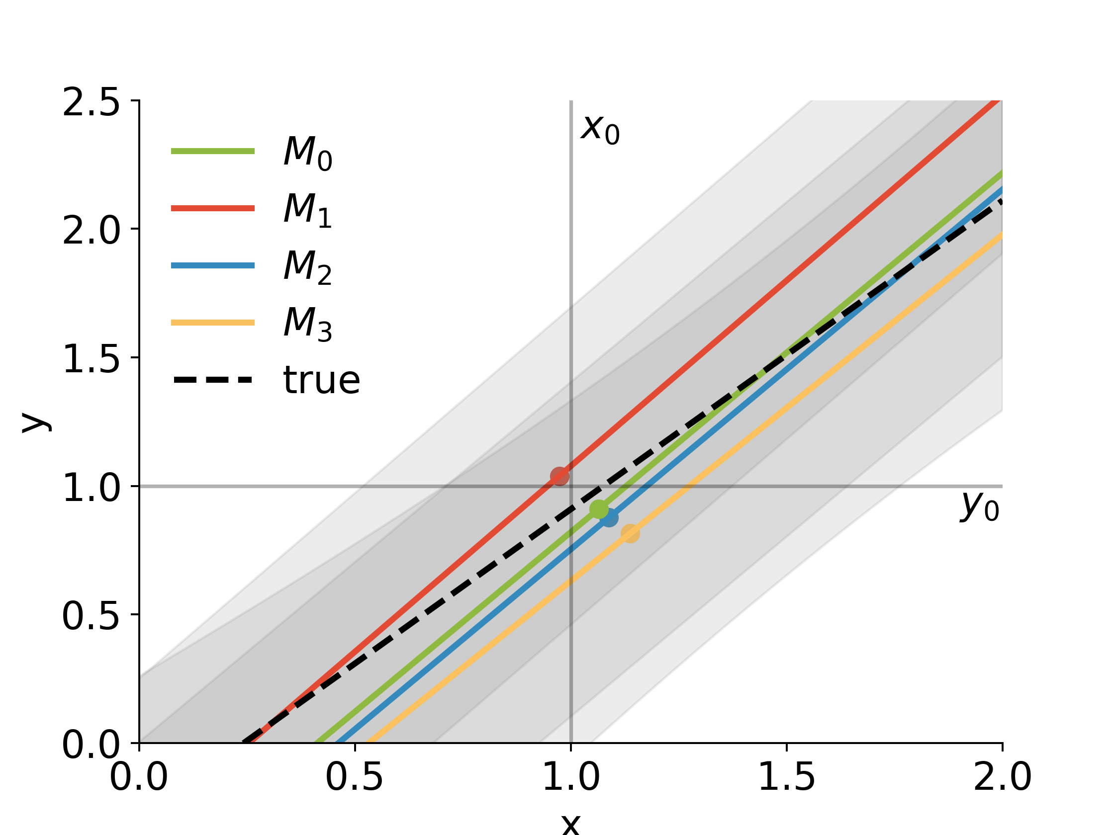
Figure 1: Optimal control example with $x_{0}=1$ and target $y_{0}=1$. The figure shows the linear predictors with 95% credible intervals from models $j=1{:}3,$ and the linear predictor from the baseline model $j=0$ (no intervals shown for $j=0$ as they are wider than the plot bounds). Model-specific optimal control points $x_{j}$ are indicated by dots.

Taking expected utilities in each ${\mathcal{M}}_{j}$ and solving for the optimal controls yields the model-specific decisions where $m_{j}$ is the posterior (to training data) mean of $\mu_{j}=\beta_{j,0}+\beta_{j,1}z_{1}+\beta_{j,2}z_{2}$ under ${\mathcal{M}}_{j}$ at the given values of $z_{1}=1.1,z_{2}=0.1.$ These optimal control values are indicated in Figure 1 in the numerical example.

BPDS adopts the univariate score functions $s_{j}(y,x)\equiv u_{j}(y,x_{j})=-(y-y_{0})^{2}/2-c_{j}(x-x_{0})^{2}/2$ with $c_{j}=cb_{j}^{2}$, i.e., the same utilities as used in each model. The following details are then implied.

• In model ${\mathcal{M}}_{j}$, the weight functions $\alpha_{j}(y|x)=\exp\{\tau(x)s_{j}(y,x_{j})\}$ are

  $$\alpha_{j}(y|x)={(2\pi/\tau(x))}^{1/2}\ N(y|y_{0},1/\tau(x))\ \exp\{-c_{j}\tau(x)(x_{j}-x_{0})^{2}/2\},$$

  where $N(y|m,v)$ is the p.d.f. of the univariate normal $N(m,v)$ evaluated at $y.$

• The resulting BPDS p.d.f. $f_{j}(y|x,{\mathcal{M}}_{j})\propto\alpha_{j}(y|x)p_{j}(y|x,{\mathcal{M}}_{j})$ is $N(m_{j}^{*}(x),v_{j}^{*}(x))$ with

  $$m_{j}^{*}(x)=v_{j}^{*}(x)\{m_{j}+b_{j}x+\tau(x)v_{j}(x)y_{0}\}\quad\textrm{and}\quad v_{j}^{*}(x)=v_{j}(x)/\{1+\tau(x)v_{j}(x)\}.$$

• The $a_{j}(x)$ are given by

  $$a_{j}(x)={(2\pi/\tau(x))}^{1/2}\exp\{-c_{j}\tau(x)(x_{j}-x_{0})^{2}/2\}N(y_{0}|m_{j}+b_{j}x,v_{j}(x)+1/\tau(x)).$$

Computations to define $\tau(x)$ at any given $x$– based on a chosen target expected score $m$– are easy via Newton-Raphson optimisation. This relies on the identities

$$\frac{\partial a_{j}(x)}{\partial\tau(x)}=-\frac{a_{j}(x)}{2}(r_{j}(x)+d_{j})\quad\textrm{with}\quad r_{j}(x)=(m_{j}^{*}(x)-y_{0})^{2}+v_{j}^{*}(x)\quad\textrm{and}\quad d_{j}=c_{j}(x_{j}-x_{0})^{2},$$

and

$$\frac{\partial^{2}a_{j}(x)}{\partial\tau(x)^{2}}=\frac{a_{j}(x)}{4}\{w_{j}(x)+2d_{j}r_{j}(x)+d_{j}^{2}\},$$

where $w_{j}(x)=(m_{j}^{*}(x)-y_{0})^{4}+6(m_{j}^{*}(x)-y_{0})^{2}v_{j}^{*}(x)+v_{j}^{*}(x)^{2}.$

BPDS analysis involves specifying the target (lower bound) on the expected score. As noted above this will be anchored in the expected score under the initial mixture so that– on the defined utility scale– BPDS is defined as an extension of the initial mixture. This example uses this concept as follows. Under the initial mixture, compute the model-specific expected scores at their optimal $x_{j}$ and then take the ET target score as the maximum; i.e., $m=\max_{j=0{:}J}E_{p}[s_{j}(y,x_{j})|\mathcal{M}_{j}].$ In the numerical example here, this yields $m=-0.046$. This is just one potential way of setting $m$, the portfolio example in Section  6 provides another alternative. Reanalysis with values slightly more or less extreme than this is also of interest, of course, while the following discussion adopts this specific value.

Under the reference BPDS utility of eqn. (10), the final BPDS optimal decision $x$ maximises the expected utility in eqn. (11), i.e.,

$$\bar{U}(x) = \tau(x)\sum_{j=0{:}J}\tilde{\pi}_{j}(x)\int_{y}s_{j}(y,x)f_{j}(y|x,{\mathcal{M}}_{j})dy$$

$$= -\tau(x)\left\{(m_{f}(x)-y_{0})^{2}+v_{f}(x)+c_{f}(x)(x-x_{0})^{2}\right\}/2,$$

where $m_{f}(x),v_{f}(x)$ are the mean and variance of $y$ under $f(y|x)$ and $c_{f}(x)=\sum_{j=0{:}J}\tilde{\pi}_{j}(x)c_{j}.$

It is easy to evaluate $\tau(x)$ and $\tilde{\pi}_{j}(x)$ and hence $\bar{U}(x)$ over a grid of $x$ values; see Figures 3 and 3. Observe the variation in the inferred ET parameter $\tau(x)$ as a function of $x,$ with a minimum of around 7. A comparison uses a proper BMA analysis. The BPDS optimal is $x_{BPDS}=1.02,$ a lightly lower value than $x_{BMA}=1.09$, shrunk a little more towards the current control setting $x_{0}=1.0$ The $\tilde{\pi}_{j}(x)$ shown in Figure 3 vary substantially with $x$. By comparison, the BMA analysis assigns around $95\%$ probability on ${\mathcal{M}}_{2}$ and almost all of the rest on ${\mathcal{M}}_{3}.$ Compared to the uniform initial weights, BPDS weighs ${\mathcal{M}}_{1}$ generally more highly and down-weights the baseline distribution– a logical choice given the increased spread of the latter. ${\mathcal{M}}_{2}$ and ${\mathcal{M}}_{3}$ are more highly weighted as $x$ increases as their optimal $x_{j}$ values are higher. Table 1 shows the true synthetic resulting linear predictor $\hat{y}_{j}$ of $y$ and the implied loss under the optimal $x_{j}$ of each ${\mathcal{M}}_{j}.$ This loss is evaluated as $L(x_{j})=(\hat{y}_{j}-y_{0})^{2}+\beta^{2}(x_{j}-x_{0})^{2}$ at the underlying slope $\beta=1.2$ of the synthetic data generating model. BPDS achieves a significantly smaller loss than any other model, including the BMA approximation and the baseline.

Model	Opt $x$	$\hat{y}$	Loss	% Excess
${\mathcal{M}}_{1}$	0.97	0.88	1.60	242
${\mathcal{M}}_{2}$	1.09	1.02	1.14	143
${\mathcal{M}}_{3}$	1.14	1.07	3.26	598
baseline (${\mathcal{M}}_{0}$)	1.06	0.99	0.61	30
Equal	1.06	0.98	0.58	24
BMA	1.09	1.02	1.21	158
BPDS	1.02	0.94	0.47	—

Table 1: Optimal control example with $x_{0}=1$ and target $y_{0}=1$. For each model, decision $x$ and resulting linear predictor $\hat{y}$, the resulting empirical loss and implied percentage increase/excess relative to BPDS. Loss here is calculated as $100\{(\hat{y}-y_{0})^{2}+\beta^{2}(x-x_{0})^{2}\}$ with true/synthetic model parameter $\beta=1.2$. BPDS dominates in terms of minimising loss, substantially so over BMA as well as over Equal weighting (the initial uniform $\pi_{j}$.)

This analysis based on $c=1$ equally penalises deviations from targets on the $x$ and $y$ scales. A repeat analysis with $c=0.1$ provides expected results with $x_{BPDS}=1.10$ and resulting $y=1.03$, closer to $y_{0}$ and further from $x_{0}$ due to decreased weight on the $x-$dimension in the score/utility. BPDS further outperforms BMA in that example with the latter having an over 620% increase in loss relative to BPDS. BMA emphasises fit to the data and generally favours more conservative models, and in this case does put the majority of its weight on the model including all relevant variables. However, BMA completely eliminating the impact of ${\mathcal{M}}_{1}$ leads to a selected control $x$ value that is too far away from $x_{0}$. BPDS operates under the assumption that the prior weights incorporate all past information about model accuracy, which in this example are uniform. ${\mathcal{M}}_{1}$ is then given an increased weight under BPDS, since its forward-looking expectation generally indicates a higher score than the other models. The BPDS mixture is superior to the prior weighting: tilting towards models expected to perform well leads to an improved final decision.

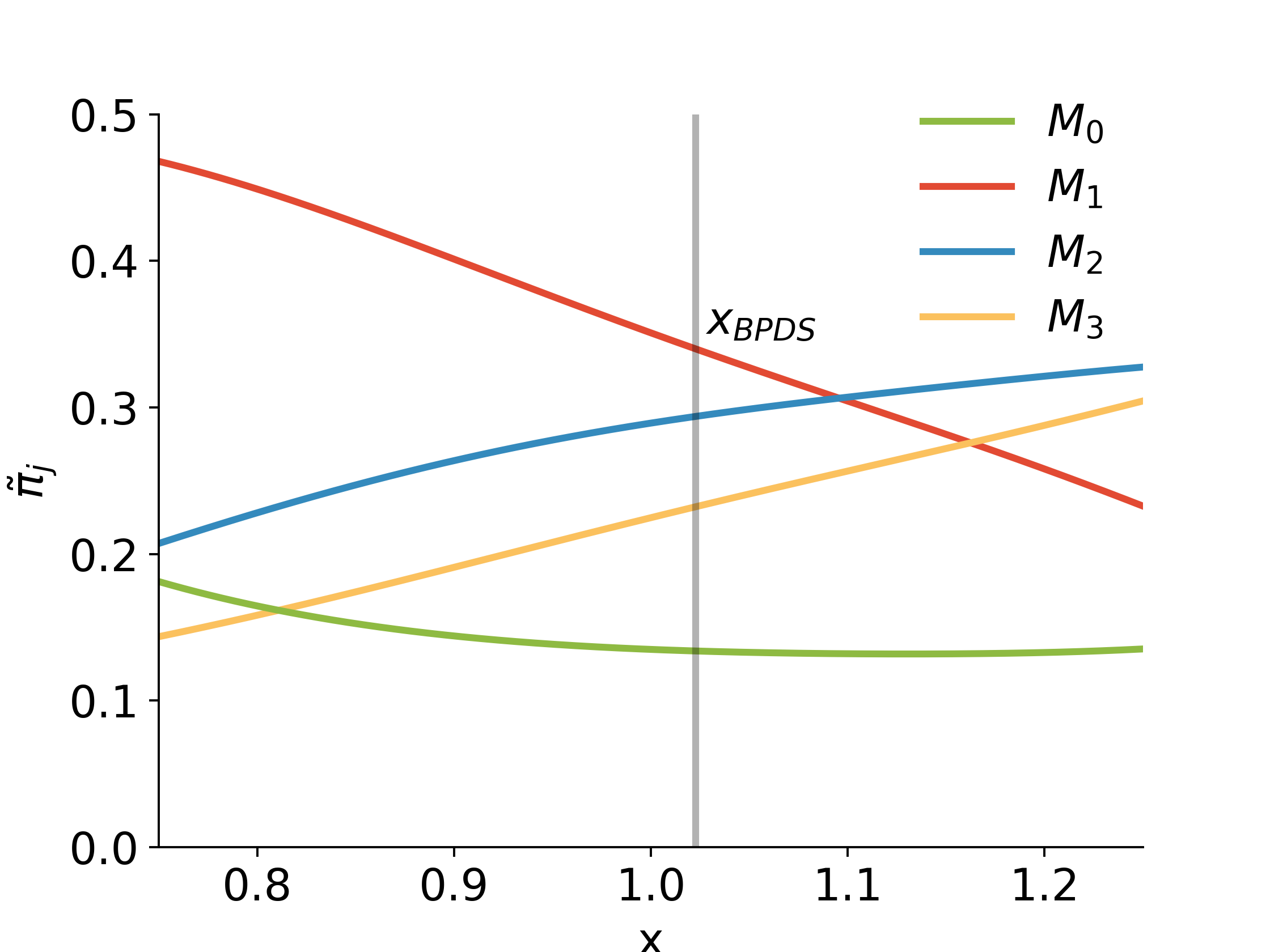
Figure 2: Optimal control example with $x_{0}=1$ and target $y_{0}=1$. ET–optimised $\tau(x)$ (left axis, blue line) and resulting expected BPDS utility (right axis, red line) across a grid of $x$, with labelled $x_{BPDS}=1.02$ that maximises the BPDS expected utility function, and $x_{BMA}=1.09$.

Figure 3: Optimal control example with $x_{0}=1$ and target $y_{0}=1$. Posterior $\tilde{\pi}_{j}(x)$ across a grid of values of $x$, with labelled $x_{BPDS}=1.02$ that maximises the expected BPDS utility function.

Example: Dynamic Portfolio Investment Decisions

Applied Setting, Data and Models

A second example concerns multivariate outcomes and time-varying models in sequential financial portfolio analysis. This involves time series of daily prices of $q=13$ assets including FX and market indices from August 2000 to the end of March 2010. On any day and based on the historical data and model analyses, the decision is to choose a portfolio weight vector to reallocate investments prior to moving to the next day. Ignoring time indices for clarity, $\mathbf{y}$ is the $1-$step ahead vector of percent returns on the $q$ assets, and the current decision is the $q-$vector of portfolio weights $\mathbf{x}$ such that the portfolio return is $\mathbf{x}^{\prime}\mathbf{y}.$ Constraints include the sum-to-one condition $\mathbf{x}^{\prime}\mathbf{1}=1$ (no additions or withdrawals of capital are allowed, and all capital must be invested). In contrast to the design example, the predictive distributions $p_{j}(\mathbf{y}|\cdot)$ and BPDS weighting functions $\alpha_{j}(\cdot|\cdot)$ do not depend on the final portfolio choice $\mathbf{x}$. The $\alpha_{j}(\cdot|\cdot)$ do, of course, depend on the ${\mathcal{M}}_{j}$–specific optimal portfolio vectors $\mathbf{x}_{j}$.

Forecasting models ${\mathcal{M}}_{j}$ are multivariate time-varying autoregressive (TV–VAR) dynamic linear models for log prices. Including the $t$ index for this discussion, the model applies to the vector $\log(\mathbf{p}_{t})$ where $\mathbf{p}_{t}$ is the vector of asset prices on day $t$. These can be transformed to the return scale using $\mathbf{y}_{t}=\mathbf{p}_{t}/\mathbf{p}_{t-1}-1$. TV–VAR models include time-varying covariance matrices addressing multivariate volatility (Aguilar and West, 2000; Irie and West, 2019; Prado et al., 2021, chap. 9 & 10). A summary of the TV–VAR model form and specification is given in the Appendix here. All models have TV–VAR order 3, reflecting expected $2{-}3$ day momentum effects in price series: each univariate series $y_{t,i}$ is predicted by all of the values of $\mathbf{y}_{t-3:t-1}$ with differing coefficients for each asset. Each model uses a state evolution discount factor $\delta=0.9995$. Models are distinguished through values of the volatility matrix discount factor $\beta$; this takes one of three values $\beta\in\{.94,.98,.995\}$, representing differing degrees of change in levels of volatility of each of the assets over time, as well as– critically for portfolio analysis– in the inter-dependencies among the assets as represented by time-varying covariances. Technical details of the roles of $(\beta,\delta)$ are given in the Appendix.

In each TV–VAR model ${\mathcal{M}}_{j}$, standard Bayesian forward-filtering analysis applies, and forecasting one-day ahead for local portfolio rebalancing (each day) uses Monte Carlo samples of the predictive distributions that map to the predictive mean vector and covariance matrix on the percent returns scale. Within each model analysis, the model-specific decisions are based on quite standard Markowitz mean-variance portfolio optimisation: this simply minimises predicted portfolio variance among sum-to-one portfolios that share a daily expected return constrained to a specified target level $r_{j}$ (see, for example, Prado et al., 2021, section 10.4.7). The set of $J=6$ BPDS model/decision pairs is defined by the use of two different target expected portfolio returns $r_{j}\in\{0.05,0.15\}$ coupled with each of the three TV–VAR models. For this example, the analyses are run “blind” and automated, with no interventions. On each day, the resulting optimised portfolio weight vector $\mathbf{x}_{j}$ is a vector of asset weights that has two constraints: they sum to one, i.e., $\mathbf{x}_{j}^{\prime}\mathbf{1}=1$, and have the specified target mean property $E(\mathbf{x}_{j}^{\prime}\mathbf{y}|{\mathcal{M}}_{j})=r_{j}$.

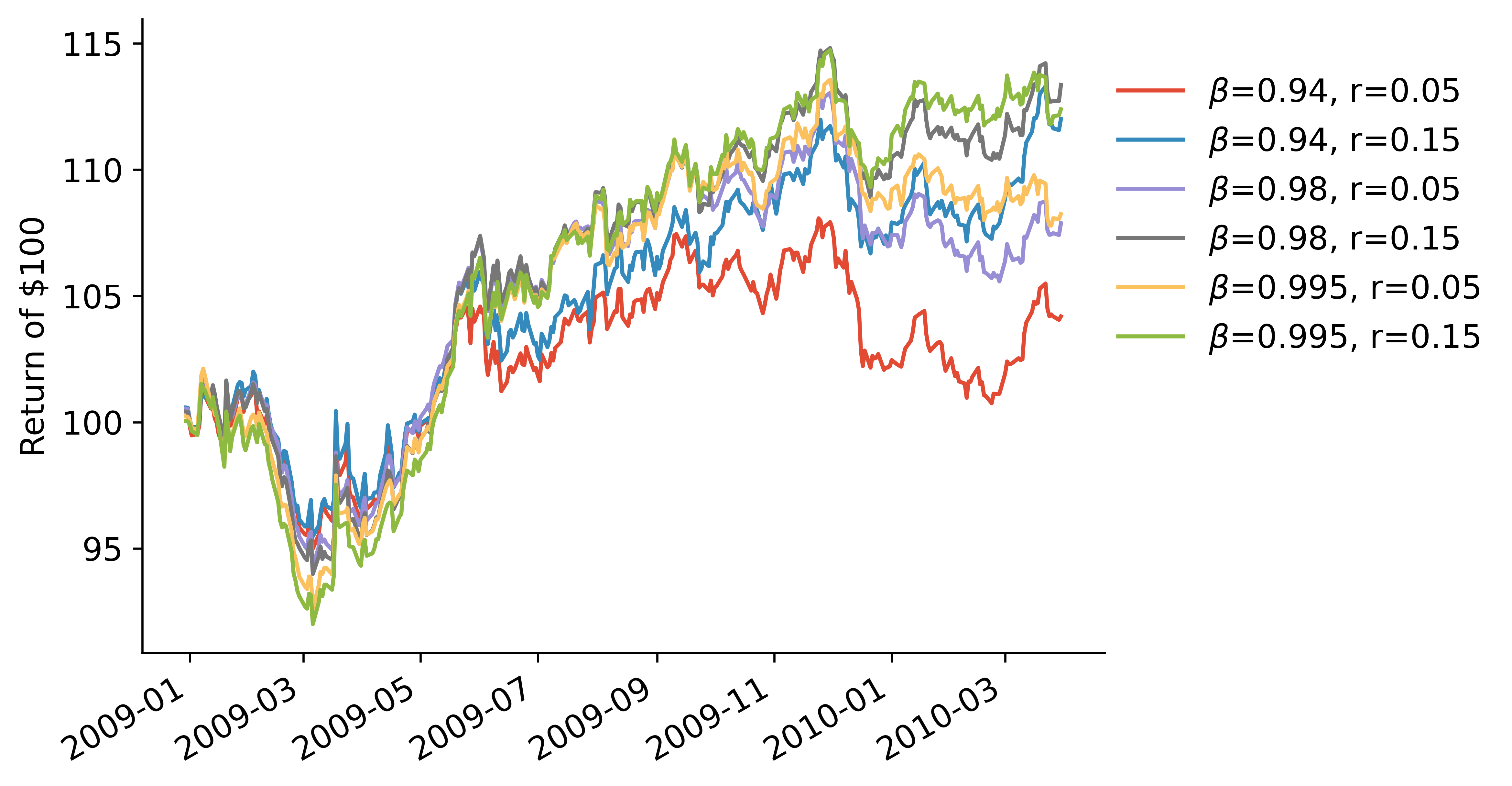
Figure 4: Returns on $100 invested from January 2009 to the end of March 2010 for $J=6$ TV–VAR models with differing volatility matrix discount factors $\beta,$ evaluated using Markowitz portfolios with two different target returns $r_{j}.$

The period of 2,195 trading days to the end of 2008 provide model training data, and the following 325 trading days to the end of March 2010 define the test period. Figure 4 shows the model-specific portfolio returns over the test period. Initial losses as national economies exit the very volatile recessionary period are followed by market stabilisation and a period of generally positive returns. Note the eventual superiority of the more stable volatility models (i.e., larger volatility discount factor $\beta$) as markets stabilise and recover from the recessionary period. This provides a good setting to evaluate BPDS, as it will ideally show more resilience to the initial downturn while taking advantage of increasing returns once model predictions and decision-outcome performance improves.

BPDS Utility-based Score

BPDS analysis adopts the bivariate score vector

$$\mathbf{s}_{j}(\mathbf{y},\mathbf{x}_{j})=[\,\mathbf{x}_{j}^{\prime}\mathbf{y},\,-(\mathbf{x}_{j}^{\prime}\mathbf{y}-m)^{2}/2\,]^{\prime}$$ (12)

for a chosen target return $m=0.1$, notably the midpoint of the model-specific potential targets. This is motivated by the classic, bounded-above risk-averse exponential utility function for return $r$ given by $V_{e}(r)=-\exp(-r/d)$ for some risk tolerance level $d>0$. A second-order Taylor series approximation around $r=m$ gives $V_{e}(r)\approx V_{q}(r)=V_{e}(r)\{1-(r-m)/d+(r-m)^{2}/2d^{2}\}.$ This is a very accurate approximation to the bounded exponential utility function across ranges of $r,m$ which correspond to realistic models for return prediction in portfolio analyses, especially for daily returns. Note that $V_{q}(r)$ is maximised at $r=m+d$. Using a univariate score $s_{j}(\mathbf{y},\mathbf{x}_{j})=\mathbf{x}_{j}^{\prime}\mathbf{y}-(\mathbf{x}_{j}^{\prime}\mathbf{y}-m)^{2}/2d$ gives $\alpha_{j}(\mathbf{y},\mathbf{x}_{j})=\exp\{\tau\mathbf{x}_{j}^{\prime}\mathbf{y}-\tau(\mathbf{x}_{j}^{\prime}\mathbf{y}-m)^{2}/2d\}$. However, using the bivariate score allows flexibility in defining the levels of risk tolerance as $d$ is implicitly specified; the bivariate score gives $\alpha_{j}(\mathbf{y},\mathbf{x}_{j})=\exp\{\tau_{1}\mathbf{x}_{j}^{\prime}\mathbf{y}-\tau_{2}(\mathbf{x}_{j}^{\prime}\mathbf{y}-m)^{2}\}/2$ which agrees with the univariate case if/when $\tau=\tau_{1}$ and $d=\tau_{1}/\tau_{2}$, and thus defines a maximising target return $m+d$ at this level of risk tolerance. The bivariate score allows more flexibility in the role of the return/risk elements and their impact in the BPDS analysis, while overlaying and replicating what the classical exponential utility univariate score defines as a special case.

Sequential Analysis and Operational BPDS for Time Series Portfolios

Recognise the sequential time series and decision setting by extending the notation to add a time subscript $t.$ In the example, this indexes working days. At any current time $t$ the model set, predictive distributions, initial model probabilities, and BPDS score vectors and targets are now all indexed by $t$ as well as model index $j;$ for example, model probabilities $\pi_{t,j}$ define weights that incorporate historical performance on all data and aspects of the analysis up to but not including time $t.$ At each time point, the BPDS analysis will take as inputs the current model summaries and define a time-specific ET vector ${\bm{\tau}}_{t}$ for the resulting BPDS mixture predictive and decisions. As $t$ evolves, the analysis will repeat.

Time-Specific Initial BPDS Probabilities and Baseline

The analysis builds on and extends prior developments of Bayesian model weighting based on historical predictive performance using AVS (Lavine et al., 2021). For each time $t,$ the current initial model probabilities are taken as $\pi_{t,j}\propto(\pi_{t-1,j})^{\gamma}\exp\{{\bm{\tau}}_{t-1}^{\prime}\mathbf{s}_{t-1,j}(\mathbf{y}_{t-1},\mathbf{x}_{t-1,j})\}$ where the AVS model discount factor $0{\ll}\gamma{<}1$ down-weights the impact of model predictive performance based on more distant past data (Zhao et al., 2016); the example here takes $\gamma=0.95$. This is a coherent extension of AVS to form an extended BPDS analysis in which the forward-looking BPDS score functions are also used as realised utilities in weighting historical model performance. Time $t=0$ model probabilities $\pi_{0,j}$ are taken as uniform. The vector score is as above in eqn. (12), now indexed by $t$ as well as $j$ to make explicit the variation in time.

The time $t$ initial mixture model defined by these AVS weights and densities $p_{t,j}(\cdot|\cdot)$ is referred to as the “AVS” model. The final aspect of model structure is the baseline. For each $t,$ each of the TV–VAR models generates a theoretical one-step ahead forecast distribution for log asset prices that is multivariate T, with parameters that are model-specific and updated in the standard forward-filtering analysis. The BPDS baseline $p_{t,0}(\cdot|\cdot)$ is taken as a T distribution with 9 degrees of freedom, the same location as the AVS mixture, and variance matrix of that of the AVS mixture inflated by $1/\delta$ with $\delta=0.135$. Consistent with the earlier discussed desiderata for the choice of baseline, this represents a neutral-but-diffuse predictive distribution relative to the current set of models in the AVS mixture. The baseline initial probability $\pi_{t,0}$ is also defined via the AVS weighting, extending the analysis to include $j=0$ giving $j=0{:}J$ dynamic models. The set of model predictive densities for time $t$ is denoted by ${\mathcal{P}}_{t}=\{p_{t,0}(\mathbf{y}_{t}|{\mathcal{M}}_{t,0}),\ldots,p_{t,J}(\mathbf{y}_{t}|{\mathcal{M}}_{t,J})\}.$

BPDS Decision Focus, Constraints and Implementation

The target score at any time point is set adaptively based on realistic assessment of expected returns and risk levels using the “current” set of models at each time. The analysis adopts $\mathbf{m}_{t}=(1.05\bar{m}_{t,1},0.9\bar{m}_{t,2})^{\prime}$ as the target score at time $t$ where the $\bar{m}_{\ast}$ elements are the expected scores under the current, time $t$ mixture over the models. This aims for a 5% greater expected return and a 10% decrease in the squared deviation from target return $m=0.1$ on each day. Further, this example setting is one in which restrictions on elements of the now time-dependent ${\bm{\tau}}_{t}$ are desirable. The elements of the score vector are obviously dependent, and it is relevant to constrain ${\bm{\tau}}_{t}$ to have positive elements so that higher expected returns and lower expected risk are rewarded. The ratio $d_{t}=\tau_{t,1}/\tau_{t,2}$ has the interpretation of a risk aversion parameter through the connection to exponential utility, and a smaller value is desirable; here the additional constraints $0<\tau_{t,1}<0.1\tau_{t,2}$ address these desiderata and additionally constrains the ET optimisation analysis for ${\bm{\tau}}_{t}$ at each time point. Note also that there is no analytic form for the $a_{t,j}$ terms in this setting; Monte Carlo analysis is used to evaluate the (time $t$ dependent extensions of) integrals in eqn. (9) within numerical optimisation to solve for ${\bm{\tau}}_{t}$.

BPDS Optimal Portfolio Decisions

With the time dependence explicit in notation, $f_{t}(\mathbf{y}_{t}|{\mathcal{P}}_{t})$ is now the one-step ahead BPDS mixture predictive density for returns from time $t-1$ to time $t.$ The operational portfolio optimisation adopts the reference utility as in Section 4.5, with the extension to time-dependence here. In this example with linear and quadratic elements of $\mathbf{s}_{t,j}(\mathbf{y}_{t},\mathbf{x}_{t})$, the expected reference utility function from eqn. (11) at time $t$ reduces to

$$\bar{U}_{t}(\mathbf{x}_{t})=\tau_{t,1}\mathbf{x}_{t}^{\prime}\mathbf{f}_{t}-\tau_{t,2}(\mathbf{x}_{t}^{\prime}\mathbf{f}_{t}-m)^{2}/2-\tau_{t,2}\mathbf{x}_{t}^{\prime}\mathbf{V}_{t}\mathbf{x}_{t}/2$$ (13)

where $\mathbf{f}_{t}$ and $\mathbf{V}_{t}$ are the forecast mean vector and variance matrix of $f_{t}(\mathbf{y}_{t}|{\mathcal{P}}_{t})$.

This is an example where additional constraints on the final decision vector $\mathbf{x}_{t}$ are relevant. First, add the usual unit-sum constraint $\mathbf{1}^{\prime}\mathbf{x}_{t}=1.$ Second, constrain portfolio decisions such that $\mathbf{x}_{t}^{\prime}\mathbf{f}_{t}=m_{t}^{*}$ for some specified target $m_{t}^{*}.$ Subject to these constraints, maximising eqn. (13) reduces to the Markowitz solution with target expected return, with a simple analytic solution for $\mathbf{x}_{t}$. The analysis here takes $m_{t}^{*}=m+d_{t}$ with risk tolerance $d_{t}=\tau_{t,1}/\tau_{t,2}$; this maximises expected utility as noted earlier in Section 6.2. With earlier discussed settings this implies that $0.1=m<m_{t}^{*}<0.2$, allowing for potential time-dependent improvements over the original target $m$.

Comparisons are with BMA–based model averaging and AVS. In each, the analysis applies Markowitz optimisation with target expected return $\sum_{j=1{:}J}\pi_{t,j}r_{t,j}$ where the $\pi_{t,j}$ are the initial mixture model weights and $r_{t,j}$ is expected return in ${\mathcal{M}}_{j}$ at time $t$. Note that BMA weights models wholly based on predictive fit to the data scored by the sequences of density values $p_{t,j}(\mathbf{y}_{t}|\mathcal{M}_{t,j})$, and does not take any account of the decision focus the models are designed to address. Thus, BMA cannot distinguish between models with identical discount factors but different expected returns $r_{t,j}$, so the portfolio weights will always evenly split weight between the two comparison targets $r_{t,j}$, giving an expected return of $0.1$. In contrast, AVS weighting accounts for the $\mathbf{x}_{t,j}$ and historical return outcomes in each model, and so differentially weights models with the same discount factor; AVS expected returns then vary over time as, of course, do those from BPDS.

Some Summary Results

For each of the three analyses– based on BPDS, BMA, and AVS, respectively– cumulative returns and empirical Sharpe ratios are shown in Figure 6. At the start of the test period, all models perform somewhat poorly through the tail-end of the recession. BPDS shows a slight advantage in this time period, but cannot completely avoid the downturn effects. However, once the economy begins to recover and information flows stabilise, BPDS is able to achieve a significantly higher return in comparison to BMA or AVS. Interestingly, basic AVS performs worse than BMA overall, which is essentially due to constraining the AVS tilting vector ${\bm{\tau}}$ to have smaller values; this is necessary in the BPDS analysis and for comparison, but leads to lack of differentially weighting “good” historical performance in basic AVS. Sharpe ratio summaries support similar conclusions. BPDS ultimately dominates both BMA and AVS. BPDS achieves increased returns without corresponding increased risk, exemplifying the prospects for prediction and decision improvements.

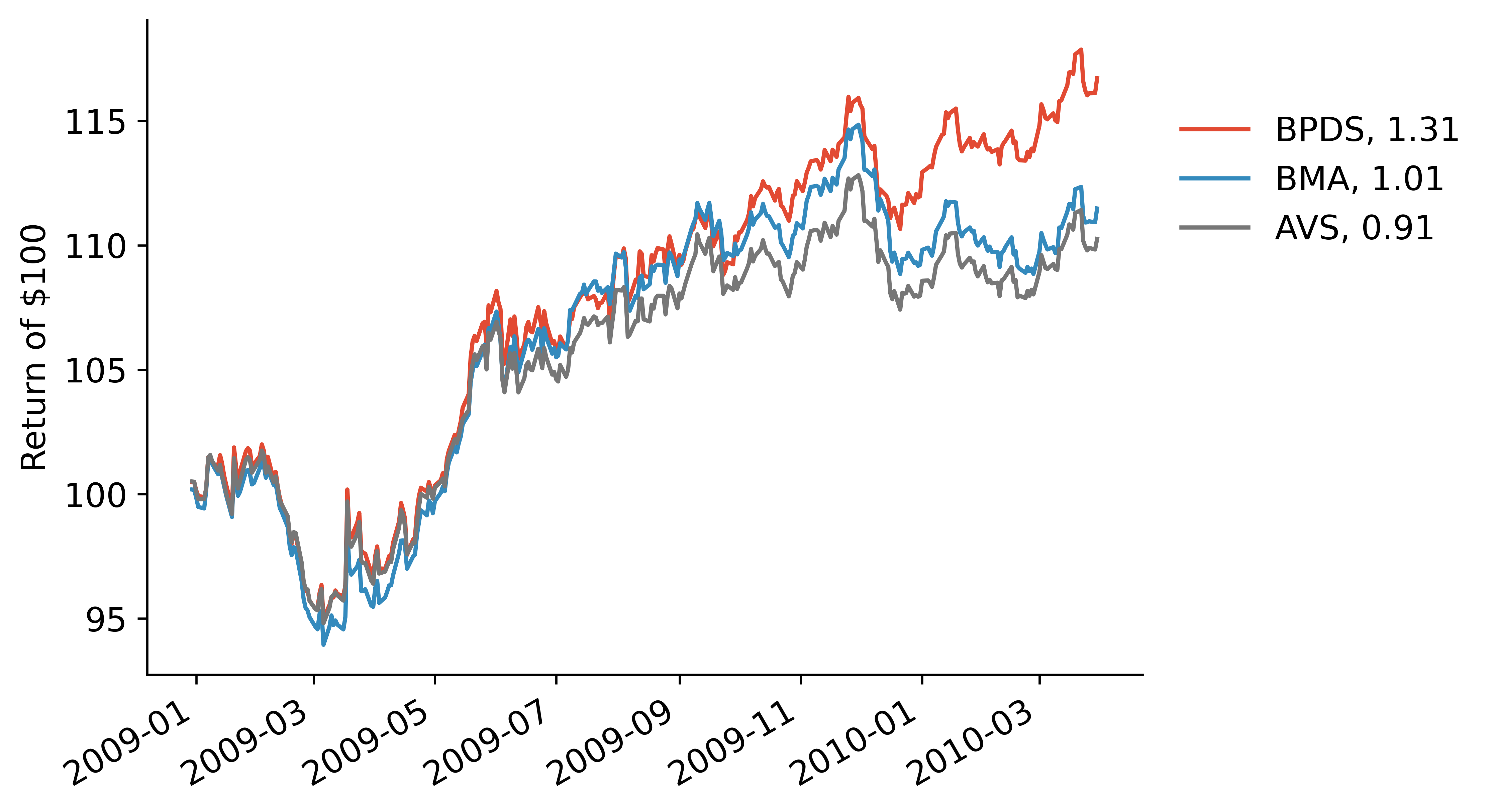
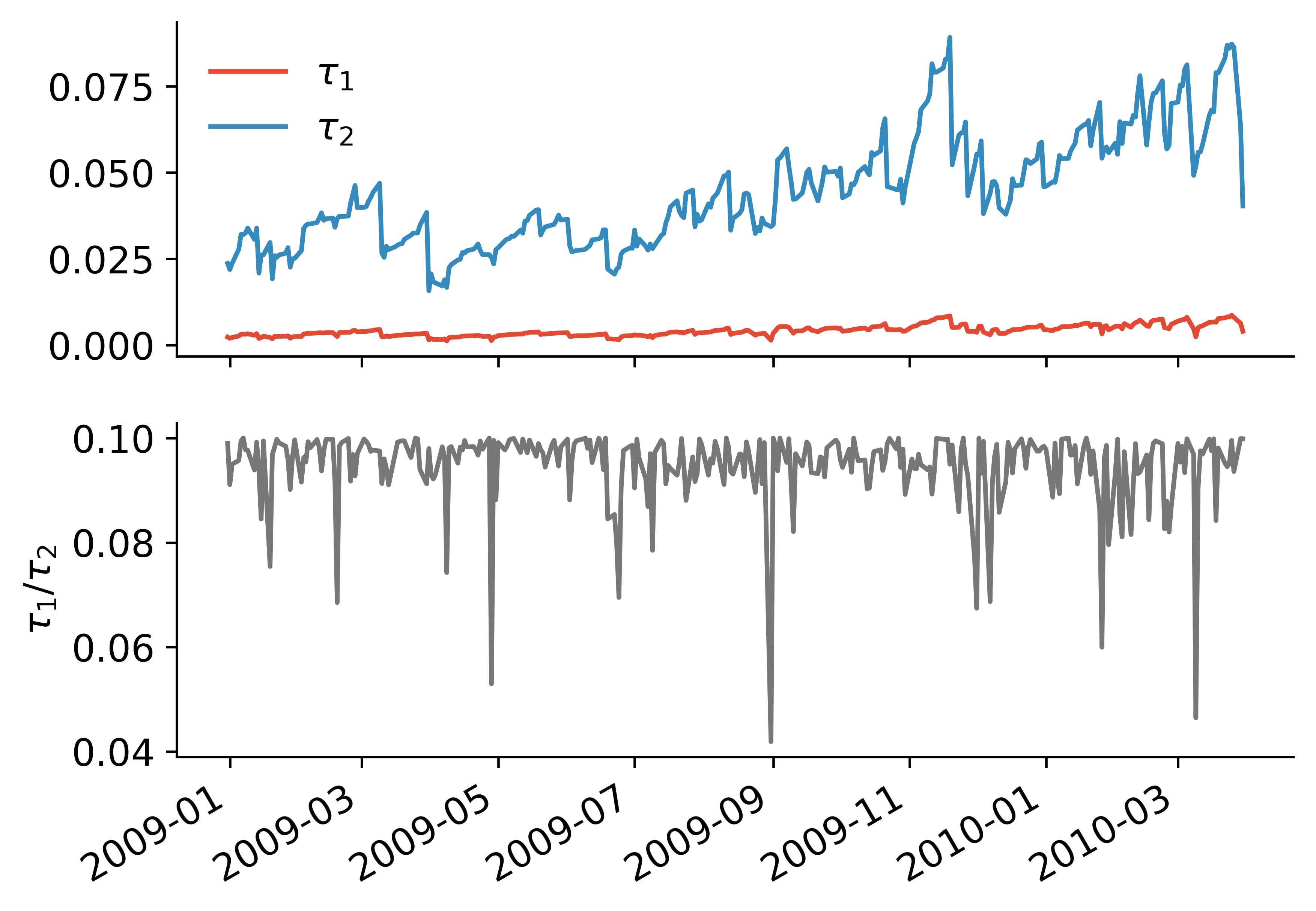
Figure 5: Returns on $100 invested from January 2009 to the end of March 2010 evaluated in each of the BPDS, BMA and AVS analyses, as well as their Sharpe ratio (see the legend, formatted as name, Sharpe). The Sharpe ratio is calculated as the annualised ratio of mean return to standard deviation of return.

Figure 6: Resulting ${\bm{\tau}}_{t}$ (upper) and ratio $\tau_{t,1}/\tau_{t,2}$ (lower) from the BPDS portfolio analysis. The latter shows that the target expected return $m+\tau_{t,1}/\tau_{t,2}$ in the BPDS analysis exhibits meaningful levels of variation throughout the time period.

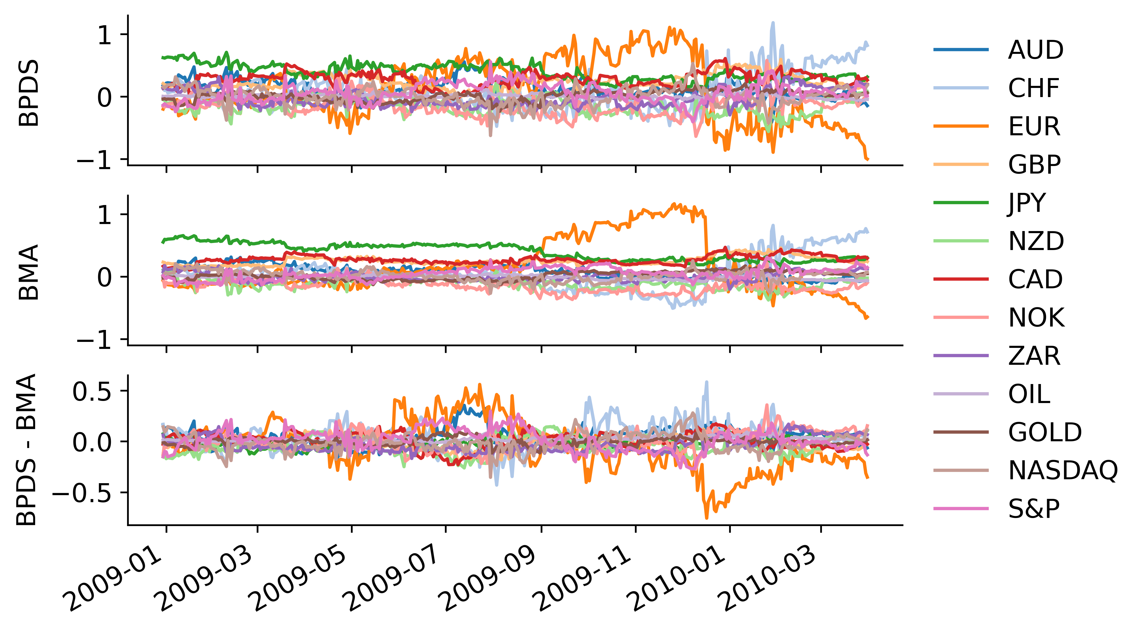
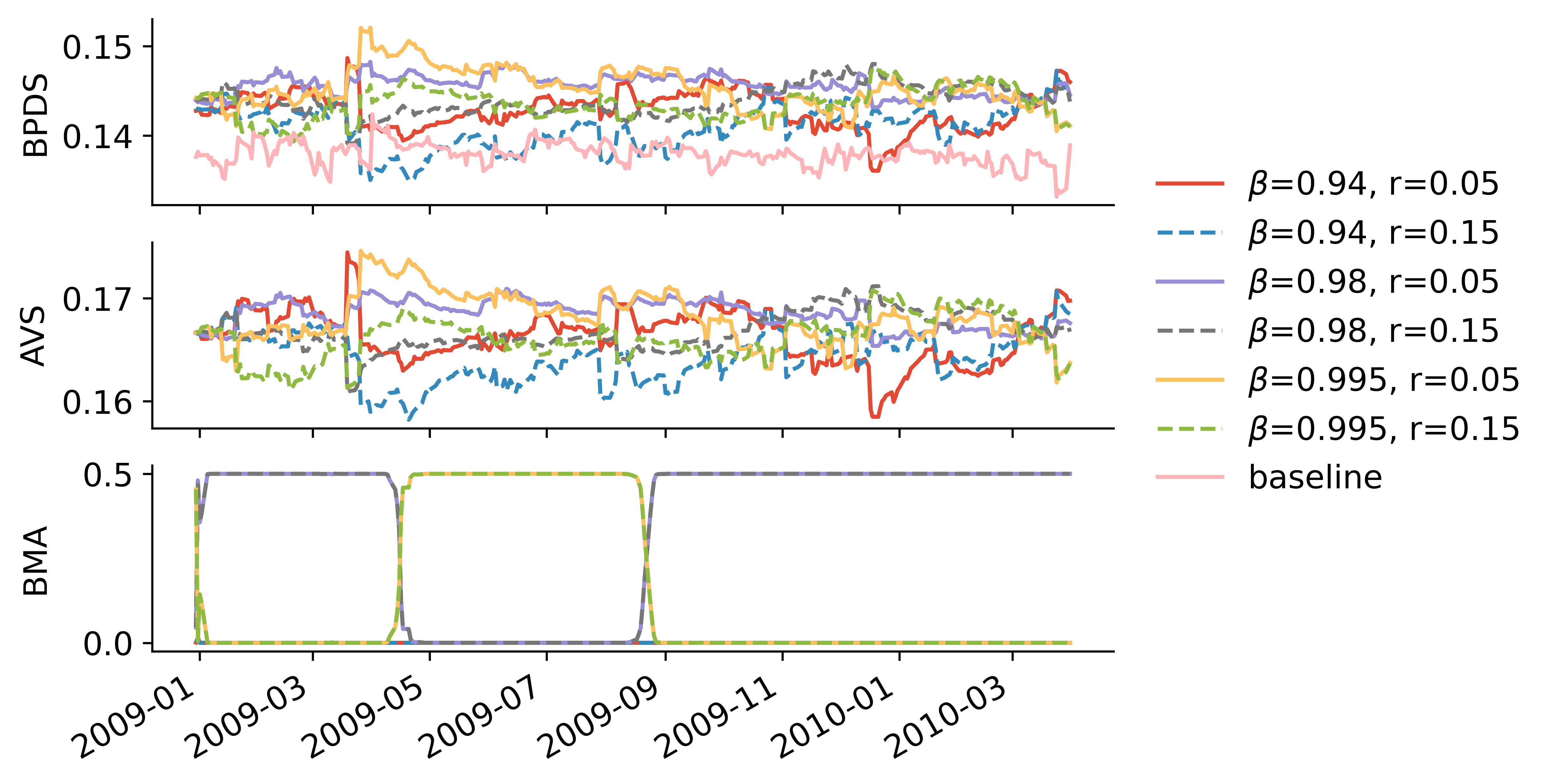
Figure 7: Time trajectories of optimised portfolio weights for each of the 13 assets in analyses based on BPDS (upper) and BMA (middle) models, and the difference of weights– BPDS minus BMA (lower).

Figure 8: Model weights $\pi^{*}_{j}$ for BPDS (upper), AVS (middle) and BMA (lower). The baseline model is only included in the BPDS analysis by definition.

Time trajectories of the optimised BPDS ${\bm{\tau}}_{t}$ vectors exhibit more variation in weightings on the second score component than the first; see Figure 6. This is partly due to the scale, as $\tau_{t,1}$ is constrained to be smaller than $\tau_{t,2}$. There are also influences from the model-specific portfolio constraints which target somewhat similar expected returns across models over the time period. That is, there is limited variation over time in expected returns (the first score vector elements) but substantially more diversity in terms of forecast uncertainty about returns (related to the second score vector element). The ratio of the two elements defines the target return for the BPDS analysis, which then does vary substantially over the time period while generally staying close to the defined $0.1$ boundary. This leads to BPDS portfolio weights being somewhat more adaptive than those from the BMA analysis (see Figure 8), while indicating that the BPDS foundation with a differing target score generally leads to higher realised scores and increased returns.

Figure 8 displays trajectories of sequentially revised portfolio weights from the BPDS and BMA analyses, and the difference in weights, BPDS minus BMA. The optimised weights have similar patterns over time, while there is generally more variation under BPDS. This decision-guided difference in the BPDS analysis partly drives small improvements in portfolio outcomes across the time period. More noticeable differences appear in mid-2009 and into 2010, particularly with respect to the weights on the Euro and, to a lesser degree, the Swiss franc. Here BPDS is more adaptive to the increasingly volatile period for the Euro linked to the developing Euro-zone sovereign debt crisis. Relative to BMA, the BPDS analysis is able to capitalise on this increased volatility and, in later 2009, begins to more aggressively short investments in the Euro. This later position is a key driver of the more evident increased returns seen in Figure 6.

Trajectories of the BPDS, BMA and AVS model probabilities are shown in Figure 8. A key feature is the typical performance of BMA. The BMA probabilities switch dramatically between favouring the two related models with $\beta=0.98$ and the two with $\beta=0.995,$ while the most adaptive models with $\beta=0.94$ receive negligible weight. The latter point is a key issue and concern in terms of time adaptability in dynamic modelling. On BPDS, note that the baseline is generally down-weighted, including during the initial period where the set of models performs relatively poorly overall. The baseline is relatively disadvantaged due to its inflated spread without a significant advantage in location over this period. Then, BPDS initially down-weights the more adaptive models in comparison to AVS due to the variance penalty in the score function rewarding more stable models. BPDS and AVS favour more stable models towards the end of the testing period as information stabilises. BPDS weights– while slightly more volatile and adaptive locally– tend to shrink AVS weights, inducing more robustness in part due to the role of the baseline.

Summary Comments

The framework of Bayesian predictive decision synthesis expands traditional thinking about evaluating, comparing and combining models to explicitly integrate decision-analytic goals. Growing from a theoretical foundation in Bayesian predictive synthesis and empirical approaches to goal-focused model uncertainty analysis, BPDS defines a theoretical basis for explicitly recognising both predictive and decision goals, integrating the intended uses of models into the model uncertainty and combination framework. Recognising and “rewarding” models through utility functions that anticipate improved decision outcomes together with predictions is the central concept. The integration with focused predictive methods, such as AVS, unites the core ideas of model scoring on past data with “outcome dependent”, anticipatory model weightings to define novel methodology. The use of entropic tilting is both foundational and enabling in implementation; ET also aids the interpretation of BPDS, important in bringing the approach to new applications.

The detailed examples highlight core aspects of the methodology and demonstrate the potential for BPDS to yield improvements in Bayesian decision analysis in two very different settings. The examples highlight the flexibility of BPDS to address a variety of prediction and decision problems, and its customisation via the use of context-dependent utility functions to define BPDS scores relevant for each applied setting. They also demonstrate that BPDS can generate interpretable outputs which may improve understanding of models differences in the decision context, in addition to generating potentially superior outcomes relative to standard model combination approaches.

The examples also note some basic implementation and computational aspects of the methodology. The use of coupled simulation and optimisation methods is generic and will be the basis for implementation in broader and larger-scale problems. BPDS predictive distributions will typically be simulated using samples from the prior mixture, delivering direct Monte Carlo approximations to integrals required in iterative solution of the optimisation problems to maximise expected utilities subject to ET and perhaps other constraints. Our design example is simple and expository; there the evaluation of decision variables across a discrete grid is easy computationally and has a convex and unique solution. In more realistic, applied design settings– such as in the use of Gaussian process regression and other reinforcement learning contexts– decision variables are multivariate, chosen BPDS utility functions may not lead to convex forms for solution, and additional constraints may be desired as in the portfolio example here. In terms of scalability of computations, note that second-order gradient methods for optimisation to define tilting vectors scale requires matrix inversions that scale cubically in the dimension of the score vectors. Alternative numerical search approaches that scale linearly might be of interest in settings models with higher-dimensional scores.

The use of AVS-style prior weights on models in the portfolio example is a setting in which the BPDS predictive distributions do not depend on the pending decision variables. Extension of AVS-style weights to settings in which this dependence exists and is key– such as in more elaborate developments of the basic optimal design example– is an open question. As with BPS, the new BPDS framework admits the use of a baseline distribution that requires specification in any application. Some desiderata are noted in Section 2.2.3 above; theoretical study of the impact of any chosen baseline represents an area for future research (relevant more broadly than BPDS). There is also theoretical interest in more foundational aspects of ET in the BPDS framework. This includes questions about the relationships between target score vectors and entropic tilting parameter vectors, delineation of problems in which ET has no solution as a result of specific choices of target scores, the roles of bounded utility functions to define scores, and theoretical implications of imposing additional constraints on the tilting parameters. On the question of choice of target scores, large deviations from that under the initial mixture will represent discarding much of the information and experience the latter is based on, so is obviously not of interest. This also relates to the question of achievable solutions for any chosen target score; while this is a matter for theoretical study, the BPDS analysis analysis can (sometimes) identify infeasible choices of target expected scores via failure of the numerical optimisation to identify implied tilting vectors. BPDS is open to including arbitrary choices of utility functions to define score vectors. The current examples involve context-specific scores, while other applications could involve more general score choices– such as scores related to aspects of probabilistic calibration (e.g. Gneiting and Raftery, 2007). Then, links with other areas of decision analysis involving multi-dimensional utilities are of interest; BPDS score vectors can reflect multiple aspects of a decision problem with the potential for conflict between dimensions. In sequential time series decision problems, as exemplified by the financial portfolio example, there are a number of open questions. Extended or alternative choices of score functions that reflect risk:reward in different ways, turnover in portfolio allocations, multi-step-ahead portfolio construction, and psychological as well as financial dimensions (e.g. Irie and West, 2019), are some general topics of interest.

Extensions of BPDS model probability weighting functions are of interest to address questions of relationships and dependencies across the set of models in the mixture. This has been a theme in recent developments of Bayesian predictive synthesis in purely predictive time series applications (McAlinn et al., 2018; McAlinn and West, 2019). The concept will apply to BPDS by extending mixture-model based BPS to allow weights on model ${\mathcal{M}}_{j}$ to depend on aspects of predictive and decision performance of other models ${\mathcal{M}}_{i}$ for $i\neq j$. There is potential practical value in this; for example, a subset of models generating very similar predictions and decisions might then each have appropriately lesser roles in the ET synthesis, accounting for the so-called herding effect (e.g. Johnson and West, 2022). There are also opportunities to explore more probabilistic choices of BPDS score functions, including score vector elements that relate to aspects of probability forecast calibration and proper scoring rules (e.g. Raftery et al., 2005). These and other extensions are open for future research.

Appendix: Multivariate TV–VAR Dynamic Models

Summaries of standard forecasting models used in the portfolio example are given here. All material is sourced from Prado et al., 2021, section 10.8; notation (including that for Wishart, inverse-Wishart, matrix normal and matrix normal-inverse Wishart distributions) is as detailed there.

Over $t=1,2,\ldots$ the $(q\times 1)-$vector time series $\mathbf{y}_{t}$ follows a random walk multivariate DLM

$$\mathbf{y}_{t}^{\prime}=\mathbf{F}_{t}^{\prime}{\bm{\Theta}}_{t}+{\bm{\nu}}_{t}^{\prime},\ \ {\bm{\nu}}_{t}\sim N(\mathbf{0},\mathbf{V}_{t}),\qquad\textrm{and}\qquad{\bm{\Theta}}_{t}={\bm{\Theta}}_{t-1}+\bm{\Omega}_{t},\ \ \bm{\Omega}_{t}\sim N(\mathbf{0},\mathbf{W}_{t},\mathbf{V}_{t}),$$

with components as follows. At time $t$:

• ${\bm{\Theta}}_{t}$ is the $(p\times q)$ time-varying state matrix, and $\mathbf{V}_{t}$ is the $(q\times q)$ time-varying volatility matrix.

• ${\bm{\nu}}_{t}$ is the $(q\times 1)$ observation error vector, and ${\bm{\Omega}}_{t}$ is the $(p\times q)$ state evolution error matrix.

• $\mathbf{F}_{t}$ is the $(p\times 1)$ regression vector of known constants and/or predictors.

• $\mathbf{W}_{t}$ is the known ($p\times p$) state evolution covariance matrix.

Write ${\mathcal{D}}_{t}$ for all past data and information prior to time $t.$ Initialise analysis using the time $t=0$ distribution $({\bm{\Theta}}_{0},\mathbf{V}_{0}|{\mathcal{D}}_{0})\sim NIW(\mathbf{M}_{0},\mathbf{C}_{0},h_{0}-q+1,\mathbf{D}_{0})$. Sequential learning and forecasting over time follows a conjugate analysis structure with, for all $t=1,2,\ldots$ the following summaries:

• Time $t-1$ posterior $({\bm{\Theta}}_{t-1},\mathbf{V}_{t-1}|{\mathcal{D}}_{t-1})\sim NIW(\mathbf{M}_{t-1},\mathbf{C}_{t-1},h_{t-1}-q+1,\mathbf{D}_{t-1})$.

• Time $t$ prior $({\bm{\Theta}}_{t},\mathbf{V}_{t}|{\mathcal{D}}_{t-1})\sim NIW(\mathbf{M}_{t-1},\mathbf{R}_{t},\beta h_{t-1}-q+1,\beta\mathbf{D}_{t-1})$ with $\mathbf{R}_{t}=\mathbf{C}_{t-1}+\mathbf{W}_{t}$. The elements $\beta,\mathbf{W}_{t}$ here are defined below.

• $1-$step ahead forecast distribution $(\mathbf{y}_{t}|{\mathcal{D}}_{t-1})\sim T_{\beta h_{t-1}}(\mathbf{f}_{t},c_{t}\mathbf{D}_{t-1})$ with $\mathbf{f}_{t}=\mathbf{M}_{t-1}^{\prime}\mathbf{F}_{t}$ and $c_{t}=\beta q_{t}/(\beta h_{t-1}-q+1).$

• Time $t$ posterior update on observing $\mathbf{y}_{t}$ gives $({\bm{\Theta}}_{t},\mathbf{V}_{t}|{\mathcal{D}}_{t})\sim NIW(\mathbf{M}_{t},\mathbf{C}_{t},h_{t}-q+1,\mathbf{D}_{t})$ with update equations

  . $\mathbf{M}_{t}=\mathbf{M}_{t-1}+\mathbf{A}_{t}\textrm{e}_{t}^{\prime},\quad\mathbf{C}_{t}=\mathbf{R}_{t}-q_{t}\mathbf{A}_{t}\mathbf{A}_{t}^{\prime},\quad h_{t}=\beta h_{t-1}+1\ \textrm{and}\ \mathbf{D}_{t}=\beta\mathbf{D}_{t-1}+\textrm{e}_{t}\textrm{e}_{t}^{\prime}/q_{t}$

  where $\textrm{e}_{t}=\mathbf{y}_{t}-\mathbf{f}_{t}$ and $\mathbf{A}_{t}=\mathbf{R}_{t}\mathbf{F}_{t}/q_{t}$ with $q_{t}=1+\mathbf{F}_{t}^{\prime}\mathbf{R}_{t}\mathbf{F}_{t}.$

The extent of time variation in the state and volatility matrices is controlled by discount factors $(\delta,\beta),$ each in $(0,1]$ and typically closer to 1. First, the state evolution covariance matrix is $\mathbf{W}_{t}=\mathbf{C}_{t-1}(1-\delta)/\delta$ based on the state discount factor $\delta.$ This simplifies details above as it implies $\mathbf{R}_{t}=\mathbf{C}_{t-1}/\delta.$ Second, the volatility matrix $\mathbf{V}_{t}$ follows a dynamic inverse Wishart evolution depending on the volatility discount factor $\beta$; this is evident above in the discounting of the Wishart degrees of freedom and scale matrix in the evolution from time $t-1$ to $t.$

TV–VAR Models

Time-varying, vector autoregressive (TV–VAR) models are special cases. A TV–VAR model of order $r$ is defined by the specification $\mathbf{F}_{t}^{\prime}=(1,\mathbf{y}_{t-1}^{\prime},\mathbf{y}_{t-2}^{\prime},\ldots,\mathbf{y}_{t-r}^{\prime}).$ Hence each univariate time series element of $\mathbf{y}_{t}$ is regression on recent past values of all $q$ univariate series up to and including lag $r$, together with an intercept term. The $i^{th}$ column of the state matrix ${\bm{\Theta}}_{t}$ then has the time-varying intercept and regression coefficients on these predictors for univariate series $i$.

Supplementary Material

Tallman and West (2022) is a supplementary document providing detailed background and theoretical developments of entropic tilting and related topics. This details the theory of ET for conditioning predictive distributions on constraints, includes new results related to connections with regular exponential families of distributions, elaborates on the relaxed entropic tilting, and provides a number of examples. Supplementary code to replicate the design example is available and will be provided in the final version.

References

- Aastveit et al. (2023) Aastveit, K. A., J. L. Cross, and H. K. van Dijk (2023). Quantifying time-varying forecast uncertainty and risk for the real price of oil. Journal of Business and Economic Statistics 41, 523–537.
- Aastveit et al. (2019) Aastveit, K. A., J. Mitchell, F. Ravazzolo, and H. K. van Dijk (2019). The evolution of forecast density combinations in economics. Oxford Research Encyclopedia of Economics and Finance. doi: 10.1093/acrefore/9780190625979.013.381.
- Aguilar and West (2000) Aguilar, O. and M. West (2000). Bayesian dynamic factor models and portfolio allocation. Journal of Business and Economic Statistics 18, 338–357.
- Amisano and Geweke (2017) Amisano, G. and J. F. Geweke (2017). Prediction using several macroeconomic models. The Review of Economics and Statistics 5, 912–925.
- Bassetti et al. (2018) Bassetti, F., R. Casarin, and F. Ravazzolo (2018). Bayesian nonparametric calibration and combination of predictive distributions. Journal of the American Statistical Association 113, 675–685.
- Bernaciak and Griffin (2022) Bernaciak, D. and J. E. Griffin (2022). A loss discounting framework for model averaging and selection in time series models. arXiv:2201.12045.
- Bernardo and Smith (1994) Bernardo, J. M. and A. F. M. Smith (1994). Bayesian Theory. Wiley, New York.
- Billio et al. (2013) Billio, M., R. Casarin, F. Ravazzolo, and H. K. Van Dijk (2013). Time-varying combinations of predictive densities using nonlinear filtering. Journal of Econometrics 177, 213–232.
- Bissiri et al. (2016) Bissiri, P. G., C. C. Holmes, and S. G. Walker (2016). A general framework for updating belief distributions. Journal of the Royal Statistical Society (Series B: Statistical Methodology) 5, 1103–1130.
- Clyde and George (2004) Clyde, M. and E. I. George (2004). Model uncertainty. Statistical Science 19, 81–94.
- Clyde and Iversen (2013) Clyde, M. and E. S. Iversen (2013). Bayesian model averaging in the open framework. In P. Damien, P. Dellaportes, N. G. Polson, and D. A. Stephens (Eds.), Bayesian Theory and Applications, pp. 483–498. Clarendon: Oxford University Press.
- DeGroot (1980) DeGroot, M. H. (1980). Improving predictive distributions. Trabajos de Estadística e Investigación Operativa 31, 385–395.
- Genest and Schervish (1985) Genest, C. and M. J. Schervish (1985). Modelling expert judgements for Bayesian updating. Annals of Statistics 13, 1198–1212.
- Geweke and Amisano (2012) Geweke, J. and G. G. Amisano (2012). Prediction with misspecified models. The American Economic Review 102, 482–486.
- Geweke and Amisano (2011) Geweke, J. F. and G. G. Amisano (2011). Optimal prediction pools. Journal of Econometrics 164, 130–141.
- Giannone et al. (2021) Giannone, D., M. Lenza, and G. E. Primiceri (2021). Economic predictions with big data: The illusion of sparsity. Econometrica 89, 2409–2437.
- Gneiting and Raftery (2007) Gneiting, T. and A. E. Raftery (2007). Strictly proper scoring rules, prediction, and estimation. Journal of the American Statistical Association 102, 359–378.
- Irie and West (2019) Irie, K. and M. West (2019). Bayesian emulation for multi-step optimization in decision problems. Bayesian Analysis 14, 137–160.
- Jiang and Tanner (2008) Jiang, W. and M. A. Tanner (2008). Gibbs posterior for variable selection in high-dimensional classification and data mining. The Annals of Statistics 5, 2207–2231.
- Johnson and West (2022) Johnson, M. C. and M. West (2022). Bayesian predictive synthesis with outcome-dependent pools. Technical Report, Department of Statistical Science, Duke University. arXiv:1803.01984.
- Kapetanios et al. (2015) Kapetanios, G., J. Mitchell, S. Price, and N. Fawcett (2015). Generalized density forecast combinations. Journal of Econometrics 188, 150–165.
- Krüger et al. (2017) Krüger, F., T. E. Clark, and F. Ravazzolo (2017). Using entropic tilting to combine BVAR forecasts with external nowcasts. Journal of Business and Economic Statistics 35(3), 470–485.
- Lavine et al. (2021) Lavine, I., M. Lindon, and M. West (2021). Adaptive variable selection for sequential prediction in multivariate dynamic models. Bayesian Analysis 16, 1059–1083.
- Lindley (1992) Lindley, D. V. (1992). Is our view of Bayesian statistics too narrow? In J. M. Bernardo, J. O. Berger, A. P. Dawid, M. H. DeGroot, and A. F. M. Smith (Eds.), Bayesian Statistics 4. Oxford University Press.
- Lindley et al. (1979) Lindley, D. V., A. Tversky, and R. V. Brown (1979). On the reconciliation of probability assessments. Journal of the Royal Statistical Society (Series A: General) 142, 146–180.
- Loaiza-Maya et al. (2021) Loaiza-Maya, R., G. M. Martin, and D. T. Frazier (2021). Focused Bayesian prediction. Journal of Applied Econometrics 36, 517–543.
- McAlinn (2021) McAlinn, K. (2021). Mixed-frequency Bayesian predictive synthesis for economic nowcasting. Journal of the Royal Statistical Society, Series C (Applied Statistics) 70, 1143–1163.
- McAlinn et al. (2020) McAlinn, K., K. A. Aastveit, J. Nakajima, and M. West (2020). Multivariate Bayesian predictive synthesis in macroeconomic forecasting. Journal of the American Statistical Association 115, 1092–1110.
- McAlinn et al. (2018) McAlinn, K., K. A. Aastveit, and M. West (2018). Bayesian predictive synthesis. Discussion of: Using stacking to average Bayesian predictive distributions, by Y. Yao et al. Bayesian Analysis 13, 971–973.
- McAlinn and West (2019) McAlinn, K. and M. West (2019). Dynamic Bayesian predictive synthesis in time series forecasting. Journal of Econometrics 210, 155–169.
- Nakajima and West (2013) Nakajima, J. and M. West (2013). Bayesian analysis of latent threshold dynamic models. Journal of Business and Economic Statistics 31, 151–164.
- Prado et al. (2021) Prado, R., M. A. R. Ferreira, and M. West (2021). Time Series: Modeling, Computation & Inference (2nd ed.). Chapman & Hall/CRC Press.
- Raftery et al. (2005) Raftery, A. E., T. Gneiting, F. Balabdaoui, and M. Polakowski (2005). Using Bayesian model averaging to calibrate forecast ensembles. Monthly Weather Review 133, 1155–1174.
- Robertson et al. (2005) Robertson, J. C., E. W. Tallman, and C. H. Whitemanng (2005). Forecasting using relative entropy. Journal of Money, Credit, and Banking 37, 383–401.
- Tallman and West (2022) Tallman, E. and M. West (2022). On entropic tilting and predictive conditioning. Technical Report, Department of Statistical Science, Duke University. arXiv:2207.10013.
- Vannitsem et al. (2021) Vannitsem, S., J. B. Bremnes, J. Demaeyer, G. R. Evans, J. Flowerdew, S. Hemri, S. Lerch, N. Roberts, S. Theis, A. Atencia, Z. B. Bouallègue, J. Bhend, M. Dabernig, L. D. Cruz, L. Hieta, O. Mestre, L. Moret, I. O. Plenković, M. Schmeits, M. Taillardat, J. V. den Bergh, B. V. Schaeybroeck, K. Whan, and J. Ylhaisi (2021). Statistical postprocessing for weather forecasts: Review, challenges, and avenues in a big data world. Bulletin of the American Meteorological Society 102, E681–E699.
- Watson and Holmes (2016) Watson, J. and C. Holmes (2016). Approximate models and robust decisions. Statistical Science 31, 465–489.
- West (1986) West, M. (1986). Bayesian model monitoring. Journal of the Royal Statistical Society (Series B: Statistical Methodology) 48, 70–78.
- West (1992) West, M. (1992). Modelling agent forecast distributions. Journal of the Royal Statistical Society (Series B: Statistical Methodology) 54, 553–567.
- West (2020) West, M. (2020). Bayesian forecasting of multivariate time series: Scalability, structure uncertainty and decisions (with discussion). Annals of the Institute of Statistical Mathematics 72, 1–44.
- West (2023) West, M. (2023). Perspectives on constrained forecasting. Bayesian Analysis, advance publication doi:10.1214/23-BA1379.
- West and Crosse (1992) West, M. and J. Crosse (1992). Modelling of probabilistic agent opinion. Journal of the Royal Statistical Society (Series B: Statistical Methodology) 54, 285–299.
- West and Harrison (1997) West, M. and P. J. Harrison (1997). Bayesian Forecasting and Dynamic Models (2nd ed.). Springer.
- Zhang (2006a) Zhang, T. (2006a). From -entropy to KL-entropy: Analysis of minimum information complexity density estimation. The Annals of Statistics 5, 2180–2210.
- Zhang (2006b) Zhang, T. (2006b). Information theoretic upper and lower bounds for statistical estimation. IEEE Transactions on Information Theory 4, 1307–1321.
- Zhao et al. (2016) Zhao, Z. Y., M. Xie, and M. West (2016). Dynamic dependence networks: Financial time series forecasting & portfolio decisions (with discussion). Applied Stochastic Models in Business and Industry 32, 311–339.