Supersolid Gap Soliton in a Bose-Einstein Condensate and Optical Ring Cavity coupling system

Abstract

The system of a transversely pumped Bose-Einstein condensate (BEC) coupled to a lossy ring cavity can favor a supersolid steady state. Here we find the existence of supersolid gap soliton in such a driven-dissipative system. By numerically solving the mean-field atom-cavity field coupling equations, gap solitons of a few different families have been identified. Their dynamical properties, including stability, propagation and soliton collision, are also studied. Due to the feedback atom-intracavity field interaction, these supersolid gap solitons show numerous new features compared with the usual BEC gap solitons in static optical lattices.

I Introduction

Due to the effect of dispersion, a wave packet would suffer a spatially spreading during its time evolution. However, when there also exists appropriate nonlinearity in the system, the dispersion spreading can be suppressed, and give rise to a non-spreading localized wave packet—soliton [1]. In a Bose-Einstein condensate (BEC) system, the nonlinearity due to attractive inter-atom contact interaction can well balance the dispersion spreading, and support a matter wave soliton, which is particularly called as bright soliton [2, 3, 4, 5, 6, 7, 8]. While for the repulsive interaction, instead of a non-spreading wavepacket, it only supports a localized atomic density dip (i.e., absence of atoms) on the background BEC density profile, which is usually named as dark soliton [9, 10, 11, 12, 13, 14, 15] (these solitons are originally studied in the field of nonlinear optics, so according to the brightness of the light pulses, they are described by the words “bright” and “dark” [16, 17, 18]). When BEC is loaded into a periodical optical lattice potential, its dispersion property can be substantially changed, as a result, even for the repulsive interaction there can also exist a bright soliton. Since the chemical potential of such a soliton falls into the energy gaps of the optical lattice potential, it is given the name of gap soliton [19, 20, 21, 22, 23, 24, 25, 26, 27, 28, 29, 30, 31, 32, 33, 34, 35, 36, 37, 38, 39]. In passing, we also mention that although gap solitons usually refer to the bright ones, there do exist dark gap solitons [40, 41, 42, 43] which are not the concerns of this paper.

Supersolid is an unusual state of matter that simultaneously behaves as both a crystalline solid and a superfluid [44, 45, 46, 47, 48]. Originally, it was predicted for helium as early as the middle of the 20th century [49, 50, 51, 52, 53], but until now it still has not been observed undoubtedly [55, 54, 56, 57, 58]. In recent years, the highly controllable atomic quantum gas brings new vitality to the supersolid studies. It has been experimentally realized in several different types of systems. The ground state of a spin-orbit coupled BEC can fall into a stripe phase exhibiting supersolid properties [59, 60, 61]. In dipolar BEC, the balance between long range dipole-dipole interaction and short range contact interaction gives rise to the emergence of arrays of quantum droplets, i.e. dipolar supersolid [62, 63, 64, 65, 66, 67, 68]. The cavity-mediated interaction also can lead to BEC supersolid. Two different schemes have already been experimentally reported, one of them couples the BEC to two crossed linear optical cavities [69, 70], while the other one uses a ring cavity [71, 72].

In this work, we are interested in the driven-dissipative supersolid BEC realized by the ring cavity scheme, for details of the physical model see section II or the original paper [71]. In this scheme, the BEC collectively scatters the pumping photons into the cavity, and results in a superradiant optical lattice, which backwardly drives the BEC into a supersolid state. As having been pointed out in the first paragraph of this section, the simultaneous existence of an optical lattice and interaction nonlinearity would lead to gap solitons in BEC. In this vein of thought, we propose that there would exist supersolid gap solitons in a BEC and ring cavity coupling system. The main objectives of this work are finding out such soliton solutions, and studying their basic properties.

The rest contents of this paper are organized as follows: In section II, we briefly describe the considering system, and present the theoretical formulas to handle its steady state and dynamical evolution. The next section III shows the main results of this paper. It is split into four subsections, which deal with the gap soliton solutions (III.1), their stability (III.2), mobility (III.3) and collision (III.4) properties respectively. At last, we summarize the paper in section IV.

II Model

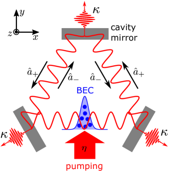
Figure 1: Schematic diagram of the considering atomic BEC and optical ring cavity coupling system. A quasi-one-dimensional BEC is loaded in an optical ring cavity along its axis. By transversely pumping the BEC using a standing wave laser (pumping strength $\eta$), light fields are built up in the cavity due to superradiant scattering of pumping photons into the two counterpropagating ring cavity optical modes ($\hat{a}_{\pm}e^{\pm ik_{c}x}$), and reach a steady state on account of the cavity loss (loss rate $\kappa$). Interference between lights of the two cavity modes forms an optical lattice. Backwardly, this optical lattice drives the BEC to a supersolid gap soliton state [71].

As schematically shown in figure 1, in this work we consider an atomic BEC and optical ring cavity coupling system. The BEC is loaded in the ring cavity along the cavity axis, and is tightly trapped in the transverse ($y,z$) direction, such that only the longitudinal ($x$) direction dynamics need to be considered. When transversely illuminating a standing-wave laser on the BEC atoms (Rabi frequency $\Omega_{0}$ and detuning $\Delta_{a}$), light fields are built up in the cavity due to the scattering of pumping photons into the two counterpropagating ring cavity optical modes ($\hat{a}_{\pm}e^{\pm ik_{c}x}$ with $\hat{a}_{\pm}$ being the annihilation operators and $k_{c}$being the wavenumber). Backwardly, the induced cavity light fields will also interact with the BEC atoms (strength ${\cal G}_{0}$). Such a system can be described by Hamiltonian [71]

$$\hat{H} =-\hbar\Delta_{c}\left(\hat{a}_{+}^{\dagger}\hat{a}_{+}+\hat{a}_{-}^{\dagger}\hat{a}_{-}\right)+\int\hat{\psi}^{\dagger}\left(x\right)H_{a}\hat{\psi}\left(x\right)dx$$

$$+\frac{1}{2}\int\hat{\psi}^{\dagger}\left(x\right)\hat{\psi}^{\dagger}\left(x^{\prime}\right)V\left(x-x^{\prime}\right)\hat{\psi}\left(x^{\prime}\right)\hat{\psi}\left(x\right)dxdx^{\prime},$$ (1)

where $\hbar$ is the Planck constant, $\Delta_{c}$ is the detuning between the cavity modes and pump laser, $\hat{\psi}$ is the field operator of the BEC. The first term describes the two counter-propagating cavity modes. The last term describes the interaction between BEC atoms. Considering the one-dimensional effective contact interaction [73], it is $V\left(x-x^{\prime}\right)=g\delta\left(x-x^{\prime}\right)$, where $g=2\hbar\omega_{\bot}a_{s}$ describes the interaction strength, with $a_{s}$ being the s-wave scattering length, $\omega_{\bot}$ referring to the frequency of transverse confinement harmonic potential. When $g<0$, it represents an attractive interaction, while for $g>0$, it is a repulsive interaction. In this work, we consider the case of repulsive interaction. The middle term accounts for the kinetic and optical potential energy of the BEC, $H_{a}$ is the corresponding single particle Hamiltonian

$$H_{a} =\frac{\hat{p}_{x}^{2}}{2m}+\hat{V}_{ac}+\hat{V}_{ap},$$ (2)

with

$$\hat{V}_{ac}=\hbar U\!\left[\hat{a}_{+}^{\dagger}\hat{a}_{+}+\hat{a}_{-}^{\dagger}\hat{a}_{-}+\left(\hat{a}_{+}^{\dagger}\hat{a}_{-}e^{-2ik_{c}x}+\mathrm{h.c.}\right)\right],$$ (3)

$$\hat{V}_{ap}=\hbar\eta\left(\hat{a}_{+}e^{ik_{c}x}+\hat{a}_{-}e^{-ik_{c}x}+\mathrm{h.c.}\right).$$ (4)

Here, $m$ is the atomic mass, $\hat{p}_{x}=-i\hbar\partial_{x}$ is the momentum operator along the $x$ direction, hence $\hat{p}_{x}^{2}/(2m)$ is the kinetic energy term. The optical potential can be split into two parts. The part caused by two-photon scattering between the two cavity modes is denoted as $\hat{V}_{ac}$, its strength is $\hbar U=\hbar\mathcal{G}_{0}/\Delta_{a}$. The other part $\hat{V}_{ap}$ is caused by two-photon scattering between pump and cavity modes, and its strength is $\hbar\eta=\hbar\mathcal{G}_{0}\Omega_{0}/\Delta_{a}$. In other words, this term describes the pumping of the system, so $\eta$ would also be called an effective pumping strength. In the following contents, we will use the natural unit $m=\hbar=k_{c}=1$ for simplicity of formulae.

Within the mean-field theory [74], the quantum operators are approximated by their mean values. The dynamical equations governing these mean-field variables can be obtained by taking mean values of the corresponding Heisenberg equations, and they are

$$i\frac{\partial}{\partial t}\alpha_{\pm}=\left(-\Delta_{c}+UN-i\kappa\right)\alpha_{\pm}+UN_{\pm 2}\alpha_{\mp}+\eta N_{\pm 1},$$ (5)

$$i\frac{\partial}{\partial t}\psi=\left[-\frac{1}{2}\frac{\partial^{2}}{\partial x^{2}}+\mathcal{V}_{\mathrm{eff}}\left(x\right)\right]\psi+\left|\psi\right|^{2}\psi,$$ (6)

with

$$N=\int\left|\psi\left(x\right)\right|^{2}dx,$$ (7)

$$N_{\pm 1}=\int\left|\psi\left(x\right)\right|^{2}e^{\mp ix}dx,$$ (8)

$$N_{\pm 2}=\int\left|\psi\left(x\right)\right|^{2}e^{\mp 2ix}dx,$$ (9)

$$\mathcal{V}_{\mathrm{eff}}\left(x\right)=\mathcal{V}_{ac}\left(x\right)+\mathcal{V}_{ap}\left(x\right),$$ (10)

$$\mathcal{V}_{ac}=U\left(\left|\alpha_{+}\right|^{2}+\left|\alpha_{-}\right|^{2}\right)+U\left(\alpha_{+}^{*}\alpha_{-}e^{-2ix}+\mathrm{c.c.}\right),$$ (11)

$$\mathcal{V}_{ap}=\eta\left(\alpha_{+}e^{ix}+\alpha_{-}e^{-ix}+\mathrm{c.c.}\right),$$ (12)

being some auxiliary quantities to make the dynamical equations compact. Here, we have introduced the cavity loss with rate $\kappa$ phenomenologically. And, we also have scaled the BEC wave function with the inter-atom interaction character length $l=\omega_{\bot}a_{s}m/\left(2\hbar k_{c}^{2}\right)$, $\psi\rightarrow\text{$\psi$}/\sqrt{l}$, therefore in equation (6) the coefficient before the nonlinear interaction term is simplified to 1. Under such a scaling, the normalization constant $N$ should be interpreted as a scaled atom number. However, without leading to any misunderstanding, literally we will still call it “atom number” for convenience in the following contents.

Due to the balance between the pumping and cavity loss, the system will reach a steady state which can be mathematically obtained by letting $\partial_{t}\alpha_{\pm}=0$, and $\psi\left(x,t\right)=\psi\left(x\right)e^{-i\mu t}$ with $\mu$ being the chemical potential. Inserting them into equations (5) and (6), one gets the following time-independent equations for steady state

$$\mu\psi\left(x\right)=\left[-\frac{1}{2}\frac{\partial^{2}}{\partial x^{2}}+\mathcal{V}_{\mathrm{eff}}\left(x\right)\right]\psi\left(x\right)+\left|\psi\left(x\right)\right|^{2}\psi\left(x\right),$$ (13)

$$\alpha_{+}=-\frac{\left(-\Delta_{c}+UN-i\kappa\right)\eta N_{+1}-\eta UN_{+2}N_{-1}}{\left(-\Delta_{c}+UN-i\kappa\right)^{2}-U^{2}N_{-2}N_{+2}},$$ (14)

$$\alpha_{-} =-\frac{\left(-\Delta_{c}+UN-i\kappa\right)\eta N_{-1}-\eta UN_{-2}N_{+1}}{\left(-\Delta_{c}+UN-i\kappa\right)^{2}-U^{2}N_{-2}N_{+2}}.$$ (15)

We see that the BEC feels an optical lattice potential from the light fields. Since we are considering a running wave ring cavity, the location of this optical lattice is not predetermined by the cavity mirrors, and spontaneously breaks the continuous translation symmetry. This optical lattice will further modulate the BEC atomic density, that is, it will drive the BEC to a spatially periodical supersolid state [71, 72]. For some examples of such states, one can see figure 2.

It is well known that when BEC with repulsive contact interaction is loaded in an optical lattice, even though the system is not well bounded, a kind of localized wavepacket, i.e., gap soliton, can also exist due to the balance between repulsive interaction and anomalous dispersion [22]. Here, a supersolid optical lattice is also built up, thus we guess that gap soliton would also exist in the now considering supersolid system. Next, we try to find such supersolid gap soliton solutions, and examine their stability, mobility, and collision properties.

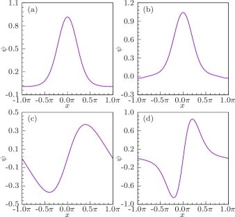
Figure 2: Examples of spatially periodical supersolid states. Only one spatial period is considered here. Chemical potentials corresponding to these states are respectively $\mu=-3.10$ (a), $-3.04$ (b), $0.55$ (c), and $-1.31$ (d), i.e., the same as those in panels (b,f) of figure 3, and panels (b,e) of figure 4. Parameters used are $\Delta_{c}=-1$, $U=-0.5$, $\kappa=10$, $\eta=15$ (this set of parameters will be used all along this paper).

III Results

III.1 Gap Soliton Solutions

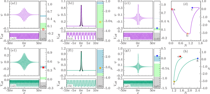
Figure 3: Fundamental gap solitons in the first (a-d) and second (e-h) energy gaps. Panels (a1-c1) and (e1-g1): wave functions $\psi\left(x\right)$ of the fundamental gap solitons. In panels (b1,f1), the black points represent the periodical supersolid states [which have previously been shown in panels (a,b) of figure 2] with the same chemical potential. Panels (a2-c2) and (e2-g2): corresponding effective optical lattice potentials $V_{\mathrm{eff}}\left(x\right)$. Panels (a3-c3) and (e3-g3): corresponding energy band structures. The gray filled region is the semi-infinite energy gap, the light-green filled region is the first energy gap, the light-blue filled region is the second energy gap, while the unfilled regions are the energy bands (some of the energy bands and gaps are too narrow to be seen very clearly). The colored points mark the chemical potential $\mu$ of the corresponding solutions. In panels (a,e), the chemical potentials lie close to the lower edge of the gap; in panels (b,f), they lie deep in the gap; and in panels (c,g), they lie near the upper edge of the gap. Panels (d) and (h): relation between chemical potential $\mu$ and atom number $N$ for fundamental gap soliton in the first (d) and second (h) energy gaps. The values of ($N,\mu$) corresponding to solutions of panels (a-c) and (e-g) are marked on the curve with the colored points which have point style the same as those in panels (a3-c3) and (e3-g3), and at the same time also explicitly labeled.

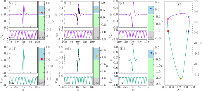
Figure 4: Sub-fundamental gap solitons in the second energy gap. Panels (a1-f1), (b2-f2), (a3-f3) and (g) are wavefunctions, effective optical lattice, energy band structure and $N$-$\mu$ curve respectively, and they are plotted the same way as figure 3. In panels (b1,e1), the black points represent the periodical supersolid states [which have previously been shown in panels (c,d) of figure 2] with the same chemical potential. The $N$-$\mu$ curve of this family of soliton is a closed loop, the upper and lower part is plotted with violet and green color respectively. The solutions of panels (a-c) have values of ($N,\mu$) on the upper part of the $N$-$\mu$ loop, while the solutions of panels (d-f) have values of ($N,\mu$) on the lower part, as labeled in panel (g).

We find gap soliton by numerically solving the discretized version (the derivative is approximated by second-order central difference) of equations (13, 14, 15), starting from an initial guessing wave function $\psi_{0}=\sum_{i=1,I}A_{i}\mathrm{sech}\left[\left(x-x_{i}\right)/\sigma_{i}\right]$ , where $A_{i}$, $x_{i}$, $\sigma_{i}$ and $I$ are numerically tunable parameters. $I$ determines the number of sub-wavepackets (peaks) of the soliton, $x_{i},\sigma_{i},A_{i}$ are the location, width and amplitude of each sub-wavepacket. We expect that each sub-wavepacket will fit in a lattice site, thus $\sigma_{i}$ is typically set to a value several times smaller than the spatial period of the optical lattice (since the dimension-less optical lattice period is $2\pi$, we typically set $\sigma_{i}$ in the range of $0.3\sim 2$). Parameter $A_{i}$ is typically set to a value in the range of $0.1\sim 1$, such that the contact interaction is obvious, but smaller than the depth of optical lattice, and a self-bounded bright soliton solution would be possible. The same typical physical parameters $\Delta_{c}=-1$, $U=-0.5$, $\kappa=10$, $\eta=15$ will be used all along this paper.

In figure 3, we show some examples of fundamental soliton wavefunctions in the first [panels (a1-c1)] and second [panels (e1-g1)] energy gaps, together with their corresponding effective optical lattice potentials [panels (a2-c2; e2-g2)] and energy band structures [panels (a3-c3; e3-g3)]. When the soliton’s chemical potential lies deep in the energy gap, its wavefunction is well localized in only one lattice site [panels (b1,f1)]. As the chemical potential moves towards the edge of the energy gap, oscillating-decay tails grow out on both sides of the central peak of the wavefunction. When the chemical potential becomes very close to the gap edge, the tail grows very heavy, see panels (a1,e1; c1,g1). Compared with the close to top gap edge case [panels (c1,g1)], near the bottom edge of the energy gap, we found that the tail decays much slower, so that the height of the tail peaks becomes almost as high as the central main peak [panels (a1,e1)].

The relation between chemical potential and atom number plays an important role in studying gap solitons. It is the basis for classifying gap solitons—a distinct family of gap solitons is usually identified by a continuous $N$-$\mu$ curve [21, 26]. For the usual gap solitons in a static optical lattice, this relation is very simple. As the atom number increases, the repulsive interaction leads the chemical potential to grow gradually, i.e., $\mu$ is a monotonic increasing function of $N$ [21, 26]. Here, the optical lattice potential is built up by pumping the atomic BEC. When the quantum state of BEC changes, the optical lattice potential also changes accordingly. The potential energy will also have an affection on the chemical potential. Therefore, we found that the relationship between $N$ and $\mu$ becomes more complex, see panels (d,h) of figure 3. For the well-localized soliton with chemical potential deep in the energy gap [panels (b,f)], a deep optical lattice is produced (hence the corresponding energy gap is relatively wide), the potential energy makes the chemical potential take a large negative value. Near the edges of the energy gap [panels (a,e;c,g)], the soliton wavefunction extends much wider. According to formulas (8–15), this will lead to smaller values of $N_{\pm 1,\pm 2}$, consequently a shallower optical lattice (hence the corresponding energy gap becomes narrower) and close to zero chemical potential. Therefore, roughly speaking the $N$-$\mu$ curve takes a “V” shape, as shown in panels (d,h). In both these two panels, the right arms of the “V” shapes have a positive dependence of $\mu$ on $N$. This can be understood by the fact that as $N$ increases the repulsive interaction becomes stronger, and at the same time as moves towards the gap edge, the lattice potential also becomes shallower. These two mechanisms both lead to the positive dependence of $\mu$ on $N$. However, in these two panels, the left arms of the “V” shapes have opposite slopes. In panel (d), as $N$ increases the repulsive interaction energy will increase accordingly. Meanwhile, the induced optical lattice becomes deeper, which leads to a decrease of potential energy. Since the atom number $N$ is small in this regime, it is the decrease of potential energy that plays the main role, thus in total $\mu$ has a negative dependence on $N$. In panel (h), even for the left arm, the atom number is also considerably large, so this time the repulsive interaction energy dominants the potential energy, and the chemical potential $\mu$ will increase with the atom number $N$. Lastly, we emphasize that the above discussions are only roughly valid, the dependence of $\mu$ on $N$ is in fact very complex, in detail, we also found that the $N$-$\mu$ curves may anomalously bend near the gap edge [the right end of panel (d), and the left end of panel (h)]. This anomalous bent reflects the nonlinear feature of the superradiant optical lattice, the similar phenomenon also happens for matter-wave solitons in other nonlinear optical lattices [25].

In the second energy gap, other than the fundamental solitons, we also found another family of solitons, see figure 4. The wavefunction of this type of soliton is very similar to the first excited state of a (harmonically) trapped particle. It possesses the odd parity symmetry, at the lattice bottom the wavefunction takes a zero value, and there are two main peaks (one is positive valued, while the other is negative valued) around this zero point. We distinguish this family of solitons as sub-fundamental solitons because their wavefunctions have the same feature as the sub-fundamental solitons reported in Ref. [26], where gap solitons in a static optical lattice are studied. The ($N,\mu$) data points of this family of solitons form a closed loop, see panel (g). The chemical potential of this family of solitons can not take values very close to the gap edge, therefore their oscillating-decay tails are always not very heavy. For the same atom number $N$, the solitons with chemical potential on the upper half part of the $N$-$\mu$ curve [panels (a-c)] are wider, and at the same time have a heavier oscillating-decay tail, compared to their lower partners [panels (d-f)].

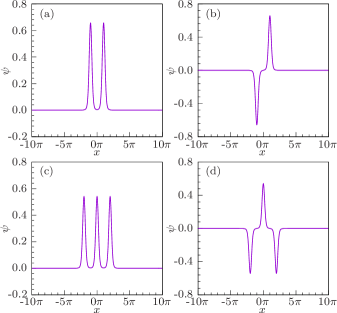
Figure 5: Examples of high order gap solitons in the first energy gap. They can be interpreted as combinations of two (a,b) or three (c,d) fundamental solitons with the same (a,c) or opposite (b,d) phases.

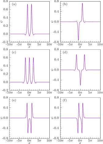
Figure 6: Examples of high order gap solitons in the second energy gap. They can be interpreted as combinations of two (a,b,e,f) or three (c,d) fundamental (a-d) or sub-fundamental (e,f) solitons with the same or opposite phases.

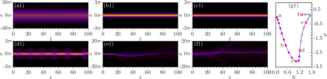
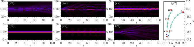
Figure 7: Stability of fundamental gap solitons in the first (a1-g1) and second (a2-g2) energy gaps. Panels (a1-f1; a2-f2): time evolutions of the atomic density $\left|\psi\left(x,t\right)\right|^{2}$ for some example solitons. Panel (g1, g2): stability of the solitons marked on the $N$-$\mu$ curve. The solid square points represent the solitons that are stable during the time evolution, while the empty square points represent the unstable ones. The ($N,\mu$) data points corresponding to panels (a1-f1; a2-f2) are specially plotted with red color, and at the same time also have been explicitly labeled.

Figure 8: Enlargements of panels (f1) and (a2) in figure 7. Originally, in figure 7, to get the overall information, these two panels are plotted in a wide spatial range. Here, to see the details of interest, they are plotted within a narrow range of $x\in\left[-5\pi,5\pi\right]$.

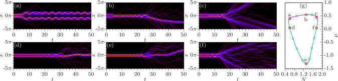
Figure 9: Stability of the sub-fundamental gap solitons in the second energy gap. The panels are plotted in a similar way as in figure 7. All these sub-fundamental solitons are unstable.

There also exist many families of high order gap solitons, which have more than one main peaks. In figure 5 (first energy gap) and figure 6 (second energy gap), some examples of two, three and four peaks solutions are shown. Comparing them with the fundamental and sub-fundamental solitons, it is straightforward to conclude that these high order solitons can be interpreted as the superposition of fundamental or sub-fundamental solitons at different lattice sites.

We also compared the spatially periodical supersolid states and the supersolid gap solitons. As shown in panels (b1,f1) of figure 3, and panel (e1) of figure 4, when the gap soliton is well localized in only one lattice site, it has almost the same shape as the periodical supersolid state with the same chemical potential. This indicates that the periodical supersolid state can be recognized as a chain of gap solitons. While for gap soliton with obvious tails around the main peak, its shape will evidently differ from the corresponding periodical solution, this can be seen from panel (b1) of figure 4. Such similarities and differences between the localized gap soliton and periodical wave have also been reported in the case of static optical lattices [32, 33, 34, 35].

III.2 Stability

The stability of these gap solitons has been checked by numerically evolving the time-dependent equations (5) and (6), with a 5% random perturbation being initially added on the soliton wavefunction $\psi_{0}$, i.e., $\psi\left(x,t=0\right)=\psi_{0}\left[1+0.05\xi\left(x\right)\right]$, with $\xi\left(x\right)$ being random numbers uniformly distributed in the range of $\left(-1,1\right)$. The corresponding atomic density is $\left|\psi\left(x,t=0\right)\right|^{2}\approx\left|\psi_{0}\right|^{2}\left[1+0.1\xi\left(x\right)\right]$, that is the atomic density is perturbed by a magnitude of 10%. However, the perturbation on total atom number is negligible, since the mean value is $\langle\xi\left(x\right)\rangle=0$. We don’t explicitly perturb the cavity optical filed, it is dynamically determined by the BEC.

Character timescales of the considering system are the dispersion time and cavity loss time. The cavity loss time is estimated by the inverse of loss rate, $\tau_{1}=1/\kappa=0.1$. The dispersion time is the spreading time of a wavepacket due to the kinetic energy term, it is related to the width of the studied wavepacket. Here character width of the gap solitons is about one lattice length $\sigma\approx\pi$, so that the dispersion time is $\tau_{2}=m\sigma^{2}/\hbar\approx 10$. Thus, for checking the stability, in the numerical simulations, we typically evolve the initial state to a final time $t=100$ (for the stable solitons) which is much longer than $\tau_{1}$ and $\tau_{2}$, or until the atomic density is substantially different from its initial profile (for the unstable solitons).

The stability results for fundamental solitons in the first energy gap are shown in panels (a1-g1) of figure 7. In panel (g1), the overall stability property is summarized on the $N$-$\mu$ curve, with the solid square points referring to stable solitons, while the empty squares for unstable ones. For detailed stability information, in panels (a1-f1), we show the time evolutions of the atomic density for some typical solitons. In panels (a1-c1), the solitons can maintain their shape during long time evolution. While, the other ones in panels (d1-f1) all lose their initial shape very quickly, however in different ways. In panel (d1), the breathing of atomic density between the main wave packet and the two tail wave packets on its two sides is excited. In panel (e1), the soliton suffers a severe spatial spreading during the evolution. In panel (f1), the soliton also suffers an overall spatially spreading, but less severe compared to that in panel (e1), because the atom density is smaller (therefore, the repulsive interaction is weaker). Another feature in panel (f1) is that the wide main wavepacket undergoes a sudden shrink at the very beginning time [this is emphasized by an enlarged graph in the top panel of figure 8], then the shrunk narrow wave packet can evolve comparatively stable for some time.

The numerical results suggest that the stability of these gap solitons roughly obeys a Vakhitov-Kolokolov (VK) criterion (a negative slope of the $N$-$\mu$ curve, $d\mu/dN<0$) [31, 36, 37, 38]. Here, we say “roughly” because of two reasons. Firstly, for the points already on the right-half of the $N$-$\mu$ curve, but still very close to the bottom of the curve, although the VK criterion is invalid, the solitons also can evolve stably for quite a long time. This would result from that the density profile of these solitons changes very slightly during the time evolution, so that the numerical simulation fails to distinguish. Secondly, at the close to gap edge anomalous bent, some points do have negative slopes, however the solitons are numerically checked to be unstable. This indicates that the VK criterion can not capture the unstable mechanism shown in panel (f1). We also would like to point out that for the normal repulsive interaction supported BEC gap solitons in static linear optical lattices, their stability obeys the anti-VK criterion by contrast [31, 36, 37, 38]. This again makes a definite difference between the supersolid gap solitons discussed here and the normal gap solitons in static optical lattices.

The stability results of fundamental solitons in the second energy gap are shown in panels (a2-g2) of figure 7. In this case, the VK criterion ($d\mu/dN<0$) is fulfilled in two places—the close to gap edge anomalous bent, and a very narrow range left to the bottom of $N$-$\mu$ curve, see panel (g2). Numerically, we found that for the anomalous bent, the VK criterion again failed to predict the right stability property, i.e., the solitons are unstable during the time evolution, for an example, see panel (a2). And around the bottom of $N$-$\mu$ curve, agree with the VK criterion (also roughly, as having been discussed in the previous paragraph), the solitons are checked to be stable, see panel (d2). All the other points on the $N$-$\mu$ curve are checked to be referring to unstable solitons. On different parts of the $N$-$\mu$ curve, the unstable mechanisms are different. Close to the stable region, the solitons are unstable because of the atomic density breathing, see panels (c2,e2). Far away from the stable region, they suffer a spatial spreading, and the larger atom number leads to the severer spreading, this is can be seen from panels (b2, f2). These two unstable mechanisms are similar to that in the first energy gap case. At last, at the anomalous bent, we also find a new unstable mechanism. As shown in panel (a2) and its enlargement in the bottom panel of figure 8, this soliton has a very heavy oscillating-decay tail, i.e., the density profile contains many small sub-wavepackets, it is unstable due to the interaction between two neighboring sub-wavepackets.

All the sub-fundamental gap solitons are numerically found to be unstable, see figure 9. Several different unstable mechanisms have been found. Firstly, the two main peaks of a sub-fundamental soliton can merge into a single peak with a loss of the atoms, see panels (d,e). Secondly, for large atom number sub-fundamental solitons, the strong repulsive interaction can lead to spatial spreading instability, see panels (c,f). Thirdly, in panel (b), for the soliton on the very top part of $N$-$\mu$ curve, at first it shrinks to another sub-fundamental soliton with two narrower density peaks (similar to its partner on the lower part of the $N$-$\mu$ curve), then these two narrower peaks merge into a single one again. Lastly, in panel (a), we found that at the beginning time the two main peaks of the sub-fundamental soliton move away from each other, and then spatial oscillations of the wavepackets are excited.

Since the high order solitons can be seen as superposition of fundamental or sub-fundamental solitons at different lattice sites, we found that they usually have a similar stability feature as their fundamental or sub-fundamental components, i.e., when the composing solitons are stable, the high order soliton is also stable and vice versa. For example, solitons (a,b,c,d) in figures 5 and 6 are found to be stable, while solitons (e,f) in figure 6 are unstable.

For comparison, we also examined the stability of normal gap solitons in static periodic potentials whose amplitude and periodicity are the same as the dynamically created optical lattice in ring cavity. We found that in such a static lattice solitons can undergo a stable evolution until the final time of the numerical simulation. So, we think that the instability of the supersolid gap solitons found here is caused by the dynamical property of the optical field.

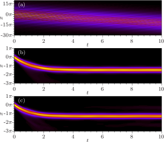
Figure 10: Mobility of the stable gap solitons. Time evolutions of the atomic density $\left|\psi\left(x,t\right)\right|^{2}$ for three different solitons with initial speed $v_{0}=4.0$ are plotted in the three panels. The three solitons are fundamental soliton near the lower edge of the first energy gap (a), deep in the first energy gap (b), and deep in the second energy gap (c) respectively. Their wavefunctions, effective optical lattice potential, and energy band structures have previously been shown in panels (a,b,f) of figure 3.

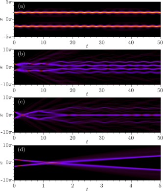
Figure 11: Collision of two gap solitons (with chemical potential deep in the first energy gap). Time evolutions of the atomic density $\left|\psi\left(x,t\right)\right|^{2}$ are plotted. From top to bottom, the initial colliding velocities are set to $v_{0}=0.5$ (a), $2.5$ (b), $3.5$ (c) and $6.0$ (d) respectively.

III.3 Mobility

In this part, we study mobility of the stable gap solitons. In a ring cavity, lights of the two counter-propagating modes can have independent phases, when their phase difference changes, the optical lattice potential produced by their interference will move. Furthermore, the light field is built up by pumping the BEC. So, it would be reasonable to expect that when the BEC wave packet moves, the optical lattice potential will move accordingly, and will put no extra force on the moving BEC, such that the BEC can move freely. However, this has been demonstrated to be only partially true. More comprehensive studies show that because the light field can not follow the BEC dynamics instantaneously, the optical lattice will fall behind the BEC for a certain distance, and will put a friction force on the BEC, as a result, the BEC will usually undergo a decelerating motion [75, 76].

To verify the above discussions, we studied the moving dynamics numerically. We give an initial velocity $v_{0}$ to the gap soliton by imprinting a phase factor $\exp\left[iv_{0}x\right]$ on its wavefunction, then examining the afterward time evolution. The results are shown in figure 10. In panels (b,c), for solitons with chemical potential deep in both the first (b) and second (c) energy gaps, we do observe a decelerating motion of the soliton wave packet. In panel (a), for the soliton with chemical potential near the gap edge, the deceleration is not obvious, it undergoes an almost free motion. This is because in this case the effective optical lattice is very weak [see panel (a2) of figure 3], as a result, the friction force is also very small, and its deceleration effect is hard to be obviously observed on the graph.

III.4 Collision

At last, we show the collision dynamics of two such supersolid gap solitons. In figure 11, taking the collisions of two solitons with chemical potential deep in the first energy gap as an example, the time evolutions of atomic density are plotted for different collision velocities. Although a single such gap soliton is movable (as having been shown in section III.3), we found that when the initial colliding velocity is small, two solitons can not approach each other, they only oscillate around their initial locations with a small amplitude, see panel (a). For the medium velocity collision [panels (b,c)], the two solitons strongly interact with each other. After some time, the two solitons either break into many small pieces [panel (b)], or merge into a single wavepacket accompanied by a scattering loss of the atoms [panel (c)]. For the large velocity collision [panel (d)], the two solitons collide similar to two classical particles, however suffering a spatial spreading. Similar collision phenomena have already been observed for non-soliton wavepackets in the same model [77], the explanations also apply here.

Strictly speaking, solitons refers to non-spreading localized wavepackets which can interact with other solitons, and emerge from the collision unchanged, except for a phase shift [1]. In this sense, the wavepackets in this work would better be called solitary waves. However, in many cases, the collision requirement is often given up, and the term soliton may be used instead of solitary wave [78], here we also follow such a relaxed definition.

IV Summary

In summary, we predict that there exist supersolid gap solitons in a BEC and optical ring cavity coupling system. We studied the system within the mean-field theory, and numerically found a few families of gap soliton solutions—fundamental gap solitons in both the first and second energy gaps, sub-fundamental gap solitons in the second energy gap, and high order gap solitons which consist of several fundamental or sub-fundamental solitons. The stability of these gap solitons has been checked by numerically simulating the time-dependent mean-field equations. The numerical results suggest that, for the fundamental solitons, their stability roughly obeys the VK criterion, i.e., usually they are stable when their chemical potential $\mu$ is negatively dependent on the atom number $N$ ($d\mu/dN<0$), however with some exceptions. All the sub-fundamental gap solitons are found to be unstable. The high order gap solitons have similar stability as their fundamental or sub-fundamental components. For the mobility property, given an initial velocity, these gap solitons usually undergo a decelerating motion due to the friction force from the light fields (the deceleration may be unobvious when friction force is weak). We also studied the two solitons collision dynamics, which are found to be strongly velocity-dependent. For small velocity collision, the two solitons can only oscillate around their initial location with a small amplitude. For medium velocity collision, the two solitons either break into many small pieces, or merge into a single wavepacket with a loss of atoms. And the large velocity collision behaves similarly to the collision of two classical particles, except that the two soliton wavepackets suffer a spatial spreading.

At last, we note that the BEC and optical ring cavity coupling system has already been realized, and supersolid phase in the system has also been identified [72]. Therefore, the supersolid gap solitons and their dynamical properties reported in this article are ready to be observed experimentally.

- [1] P. G. Drazin and R. S. Johnson, Solitons: An Introduction, 2nd ed. (Cambridge University Press, Cambridge, UK, 1989).
- [2] P. A. Ruprecht, M. J. Holland, K. Burnett, and M. Edwards, Time-Dependent Solution of the Nonlinear Schrödinger Equation for Bose-Condensed Trapped Neutral Atoms, Phys. Rev. A 51, 4704 (1995).
- [3] V. M. Pérez-García, H. Michinel, and H. Herrero, Bose-Einstein Solitons in Highly Asymmetric Traps, Phys. Rev. A 57, 3837 (1998).
- [4] L. Khaykovich, F. Schreck, G. Ferrari, T. Bourdel, J. Cubizolles, L. D. Carr, Y. Castin, and C. Salomon, Formation of a Matter-Wave Bright Soliton, Science 296, 1290 (2002).
- [5] K. E. Strecker, G. B. Partridge, A. G. Truscott, and R. G. Hulet, Formation and propagation of matter-wave soliton trains, Nature 417, 150 (2002).
- [6] K. E. Strecker, G. B. Partridge, A. G. Truscott, and R. G. Hulet, Bright Matter Wave Solitons in Bose–Einstein Condensates, New J. Phys. 5, 73 (2003).
- [7] S. L. Cornish, S. T. Thompson, and C. E. Wieman, Formation of Bright Matter-Wave Solitons during the Collapse of Attractive Bose-Einstein Condensates, Phys. Rev. Lett. 96, 170401 (2006).
- [8] T. P. Billam, A. L. Marchant, S. L. Cornish, S. A. Gardiner, and N. G. Parker, Bright Solitary Matter Waves: Formation, Stability and Interactions, in Spontaneous Symmetry Breaking, Self-Trapping, and Josephson Oscillations, edited by B. A. Malomed (Springer, Berlin, Heidelberg, 2013), pp. 403–455.
- [9] A. D. Jackson, G. M. Kavoulakis, and C. J. Pethick, Solitary Waves in Clouds of Bose-Einstein Condensed Atoms, Phys. Rev. A 58, 2417 (1998).
- [10] R. Dum, J. I. Cirac, M. Lewenstein, and P. Zoller, Creation of Dark Solitons and Vortices in Bose-Einstein Condensates, Phys. Rev. Lett. 80, 2972 (1998).
- [11] S. Burger, K. Bongs, S. Dettmer, W. Ertmer, K. Sengstock, A. Sanpera, G. V. Shlyapnikov, and M. Lewenstein, Dark Solitons in Bose-Einstein Condensates, Phys. Rev. Lett. 83, 5198 (1999).
- [12] J. Denschlag, J. E. Simsarian, D. L. Feder, C. W. Clark, L. A. Collins, J. Cubizolles, L. Deng, E. W. Hagley, K. Helmerson, W. P. Reinhardt, S. L. Rolston, B. I. Schneider, and W. D. Phillips, Generating Solitons by Phase Engineering of a Bose-Einstein Condensate, Science 287, 97 (2000).
- [13] B. P. Anderson, P. C. Haljan, C. A. Regal, D. L. Feder, L. A. Collins, C. W. Clark, and E. A. Cornell, Watching Dark Solitons Decay into Vortex Rings in a Bose-Einstein Condensate, Phys. Rev. Lett. 86, 2926 (2001).
- [14] B. Wu, J. Liu, and Q. Niu, Controlled Generation of Dark Solitons with Phase Imprinting, Phys. Rev. Lett. 88, 034101 (2002).
- [15] D. J. Frantzeskakis, Dark Solitons in Atomic Bose–Einstein Condensates: From Theory to Experiments, J. Phys. A Math. Theor. 43, 213001 (2010).
- [16] B. A. Malomed, D. Mihalache, F. Wise, and L. Torner, Spatiotemporal Optical Solitons, J. Opt. B Quantum Semiclassical Opt. 7, R53 (2005).
- [17] Z. Chen, M. Segev, and D. N. Christodoulides, Optical Spatial Solitons: Historical Overview and Recent Advances, Rep. Prog. Phys. 75, 086401 (2012).
- [18] Y. Song, X. Shi, C. Wu, D. Tang, and H. Zhang, Recent Progress of Study on Optical Solitons in Fiber Lasers, Appl. Phys. Rev. 6, 021313 (2019).
- [19] G. L. Alfimov, P. G. Kevrekidis, V. V. Konotop, and M. Salerno, Wannier Functions Analysis of the Nonlinear Schrödinger Equation with a Periodic Potential, Phys. Rev. E 66, 046608 (2002).
- [20] P. J. Y. Louis, E. A. Ostrovskaya, C. M. Savage, and Y. S. Kivshar, Bose-Einstein Condensates in Optical Lattices: Band-Gap Structure and Solitons, Phys. Rev. A 67, 013602 (2003).
- [21] N. K. Efremidis and D. N. Christodoulides, Lattice Solitons in Bose-Einstein Condensates, Phys. Rev. A 67, 063608 (2003).
- [22] B. Eiermann, Th. Anker, M. Albiez, M. Taglieber, P. Treutlein, K.-P. Marzlin, and M. K. Oberthaler, Bright Bose-Einstein Gap Solitons of Atoms with Repulsive Interaction, Phys. Rev. Lett. 92, 230401 (2004).
- [23] B. J. Da̧browska, E. A. Ostrovskaya, and Y. S. Kivshar, Interaction of Matter-Wave Gap Solitons in Optical Lattices, J. Opt. B Quantum Semiclassical Opt. 6, 423 (2004).
- [24] T. Anker, M. Albiez, R. Gati, S. Hunsmann, B. Eiermann, A. Trombettoni, and M. K. Oberthaler, Nonlinear Self-Trapping of Matter Waves in Periodic Potentials, Phys. Rev. Lett. 94, 020403 (2005).
- [25] H. Sakaguchi and B. A. Malomed, Matter-Wave Solitons in Nonlinear Optical Lattices, Phys. Rev. E 72, 046610 (2005).
- [26] T. Mayteevarunyoo and B. A. Malomed, Stability Limits for Gap Solitons in a Bose-Einstein Condensate Trapped in a Time-Modulated Optical Lattice, Phys. Rev. A 74, 033616 (2006).
- [27] O. Morsch and M. Oberthaler, Dynamics of Bose-Einstein Condensates in Optical Lattices, Rev. Mod. Phys. 78, 179 (2006).
- [28] H. Sakaguchi and B. A. Malomed, Gap Solitons in Quasiperiodic Optical Lattices, Phys. Rev. E 74, 026601 (2006).
- [29] T. Richter, K. Motzek, and F. Kaiser, Long Distance Stability of Gap Solitons, Phys. Rev. E 75, 016601 (2007).
- [30] D. L. Wang, X. H. Yan, and W. M. Liu, Localized Gap-Soliton Trains of Bose-Einstein Condensates in an Optical Lattice, Phys. Rev. E 78, 026606 (2008).
- [31] Y. Sivan, G. Fibich, B. Ilan, and M. I. Weinstein, Qualitative and Quantitative Analysis of Stability and Instability Dynamics of Positive Lattice Solitons, Phys. Rev. E 78, 046602 (2008).
- [32] Y. Zhang and B. Wu, Composition Relation between Gap Solitons and Bloch Waves in Nonlinear Periodic Systems, Phys. Rev. Lett. 102, 093905 (2009).
- [33] Y. Zhang, Z. Liang, and B. Wu, Gap Solitons and Bloch Waves in Nonlinear Periodic Systems, Phys. Rev. A 80, 063815 (2009).
- [34] T. J. Alexander and Y. S. Kivshar, Soliton Complexes and Flat-Top Nonlinear Modes in Optical Lattices, Appl. Phys. B 82, 203 (2005).
- [35] T. J. Alexander, E. A. Ostrovskaya, and Y. S. Kivshar, Self-Trapped Nonlinear Matter Waves in Periodic Potentials, Phys. Rev. Lett. 96, 040401 (2006).
- [36] H. Sakaguchi and B. A. Malomed, Solitons in Combined Linear and Nonlinear Lattice Potentials, Phys. Rev. A 81, 013624 (2010).
- [37] Y. V. Kartashov, B. A. Malomed, and L. Torner, Solitons in Nonlinear Lattices, Rev. Mod. Phys. 83, 247 (2011).
- [38] N. Dror and B. A. Malomed, Stability of Two-Dimensional Gap Solitons in Periodic Potentials: Beyond the Fundamental Modes, Phys. Rev. E 87, 063203 (2013).
- [39] J. Su, H. Lyu, Y. Chen, and Y. Zhang, Creating Moving Gap Solitons in Spin-Orbit-Coupled Bose-Einstein Condensates, Phys. Rev. A 104, 043315 (2021).
- [40] Y. S. Kivshar, W. Krlikowski, and O. A. Chubykalo, Dark Solitons in Discrete Lattices, Phys. Rev. E 50, 5020 (1994).
- [41] S. C. Cheng and T. W. Chen, Dark Gap Solitons in Exciton-Polariton Condensates in a Periodic Potential, Phys. Rev. E 97, 032212 (2018).
- [42] L. Zeng and J. Zeng, Gap-Type Dark Localized Modes in a Bose–Einstein Condensate with Optical Lattices, Adv. Photonics 1, 046004 (2019).
- [43] J. Li and J. Zeng, Dark Matter-Wave Gap Solitons in Dense Ultracold Atoms Trapped by a One-Dimensional Optical Lattice, Phys. Rev. A 103, 013320 (2021).
- [44] N. Prokof’ev, What Makes a Crystal Supersolid?, Adv. Phys. 56, 381 (2007).
- [45] S. Balibar, The Enigma of Supersolidity, Nature 464, 176 (2010).
- [46] A. B. Kuklov, N. V. Prokof’ev, and B. V. Svistunov, How Solid Is Supersolid?, Physics 4, 109 (2011).
- [47] M. Boninsegni and N. V. Prokof’Ev, Supersolids: What and Where Are They?, Rev. Mod. Phys. 84, 759 (2012).
- [48] M. H. W. Chan, R. B. Hallock, and L. Reatto, Overview on Solid 4He and the Issue of Supersolidity, J. Low Temp. Phys. 172, 317 (2013).
- [49] E. P. Gross, Unified Theory of Interacting Bosons, Phys. Rev. 106, 161 (1957).
- [50] D. J. Thouless, The Flow of a Dense Superfluid, Ann. Phys. (N. Y). 52, 403 (1969).
- [51] A. F. Andreev and I. M. Lifshitz, Quantum Theory of Defects in Crystals, J. Exp. Theor. Phys. 29, 1107 (1969).
- [52] G. V. Chester, Speculations on Bose-Einstein Condensation and Quantum Crystals, Phys. Rev. A 2, 256 (1970).
- [53] A. J. Leggett, Can a Solid Be “Superfluid”?, Phys. Rev. Lett. 25, 1543 (1970).
- [54] E. Kim and M. H. W. Chan, Probable Observation of a Supersolid Helium Phase, Nature 427, 225 (2004).
- [55] E. Kim and M. H. W. Chan, Observation of Superflow in Solid Helium, Science 305, 1941 (2004).
- [56] J. Day and J. Beamish, Low-Temperature Shear Modulus Changes in Solid 4He and Connection to Supersolidity, Nature 450, 853 (2007).
- [57] D. Y. Kim and M. H. W. Chan, Absence of Supersolidity in Solid Helium in Porous Vycor Glass, Phys. Rev. Lett. 109, 155301 (2012).
- [58] H. J. Maris, Effect of Elasticity on Torsional Oscillator Experiments Probing the Possible Supersolidity of Helium, Phys. Rev. B 86, 020502 (2012).
- [59] J. R. Li, J. Lee, W. Huang, S. Burchesky, B. Shteynas, F. Ç. Topi, A. O. Jamison, and W. Ketterle, A Stripe Phase with Supersolid Properties in Spin–Orbit-Coupled Bose–Einstein Condensates, Nature 543, 91 (2017).
- [60] T. M. Bersano, J. Hou, S. Mossman, V. Gokhroo, X.-W. Luo, K. Sun, C. Zhang, and P. Engels, Experimental Realization of a Long-Lived Striped Bose-Einstein Condensate Induced by Momentum-Space Hopping, Phys. Rev. A 99, 051602 (2019).
- [61] A. Putra, F. Salces-Cárcoba, Y. Yue, S. Sugawa, and I. B. Spielman, Spatial Coherence of Spin-Orbit-Coupled Bose Gases, Phys. Rev. Lett. 124, 053605 (2020).
- [62] L. Tanzi, E. Lucioni, F. Famà, J. Catani, A. Fioretti, C. Gabbanini, R. N. Bisset, L. Santos, and G. Modugno, Observation of a Dipolar Quantum Gas with Metastable Supersolid Properties, Phys. Rev. Lett. 122, 130405 (2019).
- [63] L. Tanzi, S. M. Roccuzzo, E. Lucioni, F. Famà, A. Fioretti, C. Gabbanini, G. Modugno, A. Recati, and S. Stringari, Supersolid Symmetry Breaking from Compressional Oscillations in a Dipolar Quantum Gas, Nature 574, 382 (2019).
- [64] M. Guo, F. Böttcher, J. Hertkorn, J. N. Schmidt, M. Wenzel, H. P. Büchler, T. Langen, and T. Pfau, The Low-Energy Goldstone Mode in a Trapped Dipolar Supersolid, Nature 574, 386 (2019).
- [65] F. Böttcher, J. N. Schmidt, M. Wenzel, J. Hertkorn, M. Guo, T. Langen, and T. Pfau, Transient Supersolid Properties in an Array of Dipolar Quantum Droplets, Phys. Rev. X 9, 011051 (2019).
- [66] L. Chomaz, D. Petter, P. Ilzhöfer, G. Natale, A. Trautmann, C. Politi, G. Durastante, R. M. W. Van Bijnen, A. Patscheider, M. Sohmen, M. J. Mark, and F. Ferlaino, Long-Lived and Transient Supersolid Behaviors in Dipolar Quantum Gases, Phys. Rev. X 9, 021012 (2019).
- [67] M. A. Norcia, C. Politi, L. Klaus, E. Poli, M. Sohmen, M. J. Mark, R. N. Bisset, L. Santos, and F. Ferlaino, Two-Dimensional Supersolidity in a Dipolar Quantum Gas, Nature 596, 357 (2021).
- [68] M. Sohmen, C. Politi, L. Klaus, L. Chomaz, M. J. Mark, M. A. Norcia, and F. Ferlaino, Birth, Life, and Death of a Dipolar Supersolid, Phys. Rev. Lett. 126, 233401 (2021).
- [69] J. Léonard, A. Morales, P. Zupancic, T. Esslinger, and T. Donner, Supersolid Formation in a Quantum Gas Breaking a Continuous Translational Symmetry, Nature 543, 87 (2017).
- [70] J. Léonard, A. Morales, P. Zupancic, T. Donner, and T. Esslinger, Monitoring and Manipulating Higgs and Goldstone Modes in a Supersolid Quantum Gas, Science 358, 1415 (2017).
- [71] F. Mivehvar, S. Ostermann, F. Piazza, and H. Ritsch, Driven-Dissipative Supersolid in a Ring Cavity, Phys. Rev. Lett. 120, 123601 (2018).
- [72] S. C. Schuster, P. Wolf, S. Ostermann, S. Slama, and C. Zimmermann, Supersolid Properties of a Bose-Einstein Condensate in a Ring Resonator, Phys. Rev. Lett. 124, 143602 (2020).
- [73] L. Salasnich, A. Parola, and L. Reatto, Effective Wave Equations for the Dynamics of Cigar-Shaped and Disk-Shaped Bose Condensates, Phys. Rev. A 65, 043614 (2002).
- [74] F. Mivehvar, F. Piazza, T. Donner, and H. Ritsch, Cavity QED with Quantum Gases: New Paradigms in Many-Body Physics, Adv. Phys. 70, 1 (2021).
- [75] J. Qin and L. Zhou, Self-Trapped Atomic Matter Wave in a Ring Cavity, Phys. Rev. A 102, 063309 (2020).
- [76] K. Gietka, F. Mivehvar, and H. Ritsch, Supersolid-Based Gravimeter in a Ring Cavity, Phys. Rev. Lett. 122, 190801 (2019).
- [77] J. Qin and L. Zhou, Collision of Two Self-Trapped Atomic Matter Wave Packets in an Optical Ring Cavity, Phys. Rev. E 104, 044201 (2021).
- [78] N. Akozbek, Optical Solitary Waves in a Photonic Band Gap Material, University of Toronto, 1998.