Universal Properties of Dense Clumps in Magnetized Molecular Clouds Formed through Shock Compression of Two-phase Atomic Gases

Abstract

We investigate the formation of molecular clouds from atomic gas by using three-dimensional magnetohydrodynamical simulations, including non-equilibrium chemical reactions, heating/cooling processes, and self-gravity by changing the collision speed $V_{0}$ and the angle $\theta$ between the magnetic field and colliding flow. We found that the efficiency of the dense gas formation depends on $\theta$. For small $\theta$, anisotropic super-Alfvénic turbulence delays the formation of gravitationally unstable clumps. An increase in $\theta$ develops shock-amplified magnetic fields along which the gas is accumulated, making prominent filamentary structures. We further investigate the statistical properties of dense clumps identified with different density thresholds. The statistical properties of the dense clumps with lower densities depend on $V_{0}$ and $\theta$ because their properties are inherited from the global turbulence structure of the molecular clouds. By contrast, denser clumps appear to have asymptotic universal statistical properties, which do not depend on the properties of the colliding flow significantly. The internal velocity dispersions approach subsonic and plasma $\beta$ becomes order of unity. We develop an analytic formula of the virial parameter which reproduces the simulation results reasonably well. This property may be one of the reasons for the universality of the initial mass function of stars.

=1 The Friends of AASTeX Collaboration

1 Introduction

The formation and evolution of molecular clouds (MCs) are crucial to set the initial condition of star formation. The formation of MCs arises from accumulation of the diffuse atomic gas, which consists of the cold neutral medium (CNM) and warm neutral medium (WNM) (Field et al., 1969).

The formation of MCs has been intensively studied by numerical simulations of atomic colliding flows (e.g., Heiles & Troland, 2005; Vázquez-Semadeni et al., 2006; Hennebelle et al., 2008; Inoue & Inutsuka, 2012). The colliding flows model accumulation of the atomic gas owing to supernova explosions (e.g., McKee & Ostriker, 1977), expansion of super-bubbles (e.g., McCray & Kafatos, 1987), galactic spiral waves (e.g., Wada et al., 2011), and large-scale colliding flows. The shock compression induces the thermal instability (Field, 1965) to form cold clouds (Hennebelle & Pérault, 2000; Koyama & Inutsuka, 2000). At the same time, a part of the kinetic energy of the colliding flows is converted into the turbulent energy of the cold clouds and intercloud gas, generating supersonic translational velocity dispersions of the cold clouds (Koyama & Inutsuka, 2002). MCs form if a sufficient amount of the gas is accumulated into the cold clouds.

Magnetic fields play a crucial role on the physical properties of MCs. Iwasaki et al. (2019) (hereafter Paper I) investigated the early stage of the molecular cloud formation through compression of the two-phase atomic gas with various compression conditions (also see Inoue & Inutsuka, 2009; Heitsch et al., 2009; Körtgen & Banerjee, 2015; Dobbs & Wurster, 2021). Paper I found that the physical properties of the post-shock layers strongly depend on the angle $\theta$ between the magnetic field and collision velocity. For a sufficiently small $\theta$, accumulation of the two-phase atomic gas drives super-Alfvénic turbulence (Inoue & Inutsuka, 2012). As $\theta$ increases, the Alfvén mach number of the turbulence decreases, and the shock-amplified magnetic field plays a major role in the dynamics of the post-shock layer.

In this paper, we investigate how the $\theta$-dependence of the turbulent properties affects the subsequent star formation by using the numerical simulations including self-gravity. We focus on the physical properties of dense clumps that are often discussed by using the virial theorem both observationally (Bertoldi & McKee, 1992) and theoretically (McKee & Zweibel, 1992). In most colliding-flow simulations, the virial theorem of dense clumps have not been discussed quantitatively. For instance, Inoue & Inutsuka (2012) investigated the physical properties of dense clumps and discuss their stability using the virial theorem, but their simulations did not include self-gravity and they did not provide quantitative discussions. We will derive an analytic estimate of each term in the virial theorem on the basis of the results of the numerical simulations.

This paper is structured as follows: In Section 2, we describe the methods and models adopted in this paper. We present our results including the global physical properties of the post-shock layers and the statistical properties of dense clumps in Section 3. Discussions are made in Section 5. Finally, we summarize our results in Section 6.

2 Methods and Models

2.1 Methods

The basic equations are the same as those used in Paper I except that self-gravity is taken into account in this work. The basic equations are given by

$$\frac{\partial\rho}{\partial t}+\frac{\partial\left(\rho v_{i}\right)}{\partial x_{i}}=0,$$ (1)

$$\frac{\partial\rho v_{i}}{\partial t}+\frac{\partial}{\partial x_{j}}\left(\rho v_{i}v_{j}+T_{ij}\right)=-\rho\frac{\partial\phi}{\partial x_{i}},$$ (2)

$$\frac{\partial E}{\partial t}+\frac{\partial}{\partial x_{i}}\left[\left(E\delta_{ij}+T_{ij}\right)v_{j}-\kappa\frac{\partial T}{\partial x_{i}}\right]=-\rho v_{i}\frac{\partial\phi}{\partial x_{i}}-{\cal L},$$ (3)

$$\frac{\partial B_{i}}{\partial t}+\frac{\partial}{\partial x_{j}}\left(v_{j}B_{i}-v_{i}B_{j}\right)=0,$$ (4)

$$\nabla^{2}\phi=4\pi G\rho,$$ (5)

and

$$T_{ij}=\left(P+\frac{B^{2}}{8\pi}\right)\delta_{ij}-\frac{B_{i}B_{j}}{4\pi},$$ (6)

where $\rho$ is the gas density, $v_{i}$ is the gas velocity, $B_{i}$ is the magnetic field, $E=\rho v^{2}/2+P/(\gamma-1)+B^{2}/8\pi$ is the total energy density, $\phi$ is the gravitational potential, $T$ is the gas temperature, $\kappa$ is the thermal conductivity, and ${\cal L}$ is a net cooling rate per unit volume. The thermal conductivity for neutral hydrogen is given by $\kappa(T)=2.5\times 10^{3}T^{1/2}$ cm^-1 K^-1 s^-1 (Parker, 1953).

The Possion equation (Equation (5)) is solved by the multigrid method that has been implemented in Athena++ by Tomida (2022, in preparation). We have implemented the chemical reactions, radiative cooling/heating, ray-tracing of FUV photons into a public MHD code of Athena++ (Stone et al., 2020) in Paper I.

We do not use the adaptive mesh refinement technique but use a uniformly spaced grid. The simulations are conducted with resolution of $2048\times 1024^{2}$, which is two times higher than that in Paper I. The corresponding mesh size is $\Delta x\sim 0.02~{}$pc. Although dense cores with $<0.1$ pc are not resolved sufficiently, the surrounding low-density regions, which is important for the MC formation and driving turbulence, are well resolved (Kobayashi et al., 2020).

To avoid gravitational collapse and numerical fragmentation, the cooling and heating processes are switched off if the local thermal Jeans length $\lambda_{\mathrm{J}}\equiv c_{\mathrm{s}}\sqrt{\pi/G\rho}$ is shorter than $4\Delta x$ (Truelove et al., 1997). Since the temperature of the dense gas is about 20 K in our results, the Truelove condition sets the maximum density $n_{\mathrm{max}}\equiv 1.4\times 10^{5}~{}\mathrm{cm}^{-3}(N_{x}/2048)^{2}(c_{\mathrm{s}}/0.3~{}\mathrm{km~{}s^{-1}})^{-2}$ above which the gas is artificially treated as the adiabatic fluid with $\gamma=5/3$.

The maximum density $n_{\mathrm{max}}$ can be reached only when self-gravity becomes important. As will be explained in Section 2.3, we consider colliding flows of the two-phase atomic gas with collision speeds of $V_{0}=5~{}\mathrm{km~{}s^{-1}}$ and $V_{0}=10~{}\mathrm{km~{}s^{-1}}$. The cold phase of the atomic gas is as dense as $n_{\mathrm{cold}}\sim 50~{}\mathrm{cm}^{-3}$. The maximum densities obtained by the shock compression are estimated to be $n_{\mathrm{cold}}(V_{0}/0.3~{}\mathrm{km~{}s^{-1}})^{2}\sim 10^{4}~{}\mathrm{cm}^{-3}$ for $V_{0}=5~{}\mathrm{km~{}s^{-1}}$ and $\sim 4\times 10^{4}~{}\mathrm{cm}^{-3}$ for $V_{0}=10~{}\mathrm{km~{}s^{-1}}$, both of which are smaller than $n_{\mathrm{max}}$.

Paper I took into account 9 chemical species (H, H₂, H⁺, He, He⁺, C, C⁺, CO, $e$) following Inoue & Inutsuka (2012). We improved the chemical networks and thermal processes following Gong et al. (2017). We consider 15 chemical species (H, H₂, H⁺, H${}_{2}^{+}$, H${}_{3}^{+}$, He, He⁺, C, C⁺, CH_x, CO, O, OH_x, HCO⁺, $e$) which are similar to those in Nelson & Langer (1999). We calculate the far-ultraviolet (FUV) flux, which causes photo-chemistry and related thermal processes, is required to be calculated at any cells. In the same way as in Paper I and Inoue & Inutsuka (2012), FUV radiation is divided into two rays which propagate along the $x$-direction from the left and right $x$-boundaries because the compression region has a sheet-like configuration, and the column densities along the $x$-direction are smaller than those in the $y$- and $z$-directions. The two-ray approximation is also adapted for calculating the escape probabilities of the cooling photons. The detailed description is found in Paper I.

The cosmic-ray ionization rate per hydrogen nucleus $\xi_{\mathrm{H}}$ varies significanly depending on regions. In this paper, we adopt the recently updated one in diffuse molecular clouds $\xi_{\mathrm{H}}=2\times 10^{-16}~{}$s^-1 (Indriolo et al., 2007, 2015; Neufeld & Wolfire, 2017), which is about ten times larger than that adopted in Paper I. We should note that the cosmic ray flux is attenuated toward the deep interior of molecular clouds, and Neufeld & Wolfire (2017) showed marginal evidence that $\xi_{\mathrm{H}}$ decreases with $A_{\mathrm{V}}$ in proportional to $A_{\mathrm{V}}^{-1}$ for $A_{\mathrm{V}}>0.5$. Our adopted value of $\xi_{\mathrm{H}}=2\times 10^{-16}~{}$s^-1 corresponds to an upper limit of the cosmic-ray ionization rate, and the gas temperature at dense regions may be slightly overestimated.

As a solver of the stiff chemical equations, we adopt the Rosenbrock method, which is a semi-implicit 4th-order Runge-Kutta scheme (Press et al., 1986). The time width $\Delta t_{\mathrm{chem}}$ required to solve the chemical reactions with sufficiently small errors can be much smaller than that of the MHD part. We integrate the chemical reactions with adaptive substepping, and the number of the substeps is determined so that a error estimated from 3rd-order and 4th-order solutions becomes sufficiently small.

2.2 A Brief Review of Paper I

Before presenting the models in this study, we here review the results of Paper I that investigated the early stage of molecular cloud formation from atomic gas by ignoring self-gravity. They performed a survey in a parameter space of ($\langle n_{0}\rangle$, $V_{0}$, $B_{0}$, $\theta$), where $\langle n_{0}\rangle$ is the mean density of the pre-shock atomic gas, $V_{0}$ is the collision velocity, and $B_{0}$ is the field strength, and $\theta$ is the angle between the collision velocity and magnetic field of the atomic gas. At a given parameter set of $(\langle n_{0}\rangle,B_{0},V_{0})$, they found that there is a critical angle $\theta_{\mathrm{cr}}$ which characterizes the physical properties of the post-shock layers. They obtained an analytic formula of the critical angle as follows:

$$\sin\theta_{\mathrm{cr}}=0.1\left(\frac{\langle n_{0}\rangle}{10~{}\mathrm{cm}^{-3}}\right)^{1/2}\left(\frac{V_{0}}{5~{}\mathrm{km~{}s^{-1}}}\right)\left(\frac{B_{0}}{3~{}\mu\mathrm{G}}\right)^{-1}.$$ (7)

• For an angle smaller than $\theta_{\mathrm{cr}}$, anisotropic super-Alfvénic turbulence is maintained by the accretion of the two-phase atomic gas. The ram pressure dominates over the magnetic stress in the post-shock layers. As a result, a greatly-extended turbulence-dominated layer is generated.

• For an angle comparable to $\theta_{\mathrm{cr}}$, the shock-amplified magnetic field weakens the post-shock turbulence, making the post-shock layer denser. The mean post-shock density has a peak around $\theta\sim\theta_{\mathrm{cr}}$ as a function of $\theta$.

• For an angle larger than $\theta_{\mathrm{cr}}$, the magnetic pressure plays an important role in the post-shock layer. Their mean densities decrease with $\theta$ and are determined by the balance between the post-shock magnetic pressure and pre-shock ram pressure (see also Inoue & Inutsuka, 2012).

2.3 Models

We consider colliding flows of the two-phase atomic gas whose mean density is $\langle n_{0}\rangle$ in the same manner as in Paper I. The collision speed is $V_{0}$, magnetic field strength is $B_{0}$ and the angle between the colliding flow and magnetic field is $\theta$. The colliding flows move in the $\pm x$ directions, and the magnetic fields are tilted toward the $y$-axis.

In order to generate the initial conditions for performing the colliding-flow simulations, the upstream two-phase atomic gas is generated using the same manner as in Paper I. We prepare a thermally unstable gas in thermal equilibrium with a mean density of $\langle n_{0}\rangle$ and a uniform magnetic field of $\mathbf{B}_{0}$ in a cubic simulation box of $-10~{}\mathrm{pc}\leq x,y,z\leq 10~{}\mathrm{pc}$ with the periodic boundary conditions in all the directions. As the initial condition, we add a velocity dispersion having a Kolmogrov spectrum of $0.64~{}\mathrm{km~{}s^{-1}}~{}(L/~{}\mathrm{pc})^{0.37}$, where $L$ is the size of regions. The initial unstable gas evolves into the two thermally stable states, or the CNM and WNM, in about one cooling timescale. We terminate the simulations at $t=8~{}$Myr or $\sim 4$ cooling timescale of the initial unstable gas. The density distribution of our upstream gas is highly inhomogeneous, where the dense CNM clumps are embedded in the diffuse WNM (see Figure 1 in Paper I).

In the colliding flow simulations, the simulation box is doubled in the $x$-direction, or $-20~{}\mathrm{pc}\leq x\leq 20\mathrm{pc}$, $-10~{}\mathrm{pc}\leq y,z\leq 10~{}\mathrm{pc}$. In the $y$- and $z$-directions, periodic boundary conditions are imposed. The $x$-boundary conditions at $x=\pm 20~{}$pc are imposed so that the initial distribution is periodically injected into the computation region from both the $x$-boundaries with a constant speed of $V_{0}$.

The model parameters are listed in Table 1. In all the models, $\langle n_{0}\rangle=10~{}\mathrm{cm}^{-3}$ is adopted. As in Paper I, we here consider the formation of MCs through accretion of HI clouds with a mean density of $\sim 10~{}\mathrm{cm}^{-3}$ (Blitz et al., 2007; Fukui et al., 2009; Inoue & Inutsuka, 2012; Fukui et al., 2017) rather than through accretion of the warm neutral medium. For all the models, the field strength $B_{0}$ is set to $3~{}\mu$G, which is roughly consistent with a typical field strength in the atomic gas (Heiles & Troland, 2005; Crutcher et al., 2010).

As a fiducial model in this paper, we consider $V_{0}=5~{}\mathrm{km~{}s^{-1}}$. In order to investigate the dependence of the results on the collision velocity, we perform additional simulations with $V_{0}=10~{}\mathrm{km~{}s^{-1}}$. Our simulations model accumulation of the atomic gas by expansion of HI shells or spiral shock waves (McCray & Kafatos, 1987; Wada et al., 2011). The critical angle for the fiducial model is $\sin\theta_{\mathrm{cr}}=0.1$ for $V_{0}=5~{}\mathrm{km~{}s^{-1}}$ and $0.2$ for $V_{0}=10~{}\mathrm{km~{}s^{-1}}$ (Equation (7)).

For each $V_{0}$, we consider cases with $\theta=0.25\theta_{\mathrm{cr}}$ and $\theta=2\theta_{\mathrm{cr}}$ as representative models of the turbulence-dominated and magnetic-pressure-dominated layers, respectively (Section 2.2). We name a model by attaching “$\Theta_{\mathrm{cr}}$” in front of a value of $\theta/\theta_{\mathrm{cr}}$ followed by “V” in front of a value of $V_{0}/1~{}\mathrm{km~{}s^{-1}}$ (Table 1).

model	$V_{0}~{}[\mathrm{km~{}s^{-1}}]$	$\theta$	$t_{\mathrm{first}}$
$\Theta_{\mathrm{cr}}0.25\mathrm{V5}$	5	$1.5^{\circ}~{}(0.25\theta_{\mathrm{cr}})$	8.3 Myr
$\Theta_{\mathrm{cr}}2\mathrm{V5}$	5	$11^{\circ}~{}(2\theta_{\mathrm{cr}})$	6.0 Myr
$\Theta_{\mathrm{cr}}0.25\mathrm{V10}$	10	$3^{\circ}~{}(0.25\theta_{\mathrm{cr}})$	8.8 Myr
$\Theta_{\mathrm{cr}}2\mathrm{V10}$	10	$24^{\circ}~{}(2\theta_{\mathrm{cr}})$	6.0 Myr

Table 1: List of the model parameters. In the rightmost column, $t_{\mathrm{first}}$ indicates the epoch when the first unstable clump is formed. In all the models, $\langle n_{0}\rangle=10~{}\mathrm{cm}^{-3}$ and $B_{0}=3~{}\mu$G are adopted.

It is useful to estimate global mass-to-flux ratios $\mu_{\mathrm{layer}}$ of the post-shock layers (Strittmatter, 1966; Mouschovias & Spitzer, 1976; Nakano & Nakamura, 1978; Tomisaka et al., 1988; Tomisaka, 2014). The total mass of the post-shock layer increases with time, following $M_{\mathrm{layer}}=2\langle\rho_{0}\rangle V_{0}L^{2}t$, where $L=20~{}\mathrm{pc}$ is the box size along the $y$- and $z-$axes. The magnetic flux held in the post-shock layer depends on direction. In the plane perpendicular to the $x$-axis ($y$-axis), the magnetic fluxes $\Phi_{x}$ ($\Phi_{y}$) is expressed as $B_{0}L^{2}\cos\theta$ ($2B_{0}V_{0}Lt\sin\theta$). The global mass-to-flux ratio is estimated as $\mu_{\mathrm{layer}}=\min(M_{\mathrm{layer}}/\Phi_{x},M_{\mathrm{layer}}/\Phi_{y})$. It increases with time as $M_{\mathrm{layer}}/\Phi_{x}\propto t$, but does not exceed $M_{\mathrm{layer}}/\Phi_{y}=\langle\rho_{0}\rangle L/(B_{0}\sin\theta)$. The global gravitational instability of the post-shock layers occurs if $\mu_{\mathrm{layer}}$ exceeds a critical value of $\mu_{\mathrm{cr}}=(2\pi\sqrt{G})^{-1}$. The ratio is given by

$$\frac{\mu_{\mathrm{layer}}}{\mu_{\mathrm{cr}}} = 4\langle n_{0}\rangle_{1}B_{3}^{-1}$$ (8)

$$\times \min\left\{V_{5}t_{10}\left(\frac{\cos\theta}{1}\right)^{-1},L_{20}\left(\frac{\sin\theta}{0.2}\right)^{-1}\right\},$$

where $\langle n_{0}\rangle_{\mathrm{1}}=\langle n_{0}\rangle/10~{}\mathrm{cm}^{-3}$, $B_{3}=B_{0}/3~{}\mu\mathrm{G}$, $V_{5}=V_{0}/5~{}$km s^-1, $L_{20}=L/20~{}$pc, and $t_{10}=t/10~{}\mathrm{Myr}$. The mass-to-flux ratios of the post-shock layers increase in proportion to time and exceed unity at $t=2.5V_{5}^{-1}~{}\mathrm{Myr}$. They continue to increase at least until $t=10~{}$Myr for the $\theta=0.25\theta_{\mathrm{cr}}$ models while they reach the maximum values of $2$ at $t=5$ Myr for model $\Theta_{\mathrm{cr}}2$V5 and $4$ at $t=2.5~{}$Myr for model $\Theta_{\mathrm{cr}}2$V10. The star formation will be suppressed for largely-inclined compressions with $\sin\theta>0.8\langle n_{0}\rangle_{10}B_{3}L_{20}$ because $M_{\mathrm{layer}}/\Phi_{y}<\mu_{\mathrm{cr}}$ unless magnetic dissipation processes, such as ambipolar diffusion and/or turbulent reconnection work.

3 Results

In this section, we show the simulation results up to $t=t_{\mathrm{first}}+0.5$ Myr, where $t_{\mathrm{first}}$ is the formation time of the first unstable clump, which will be defined in Section 3.2. In our simulations, the resolution is not high enough to resolve dense cores ($>10^{5}~{}\mathrm{cm}^{-3}$) and the thermal processes are switched-off in the regions where the Jeans condition is violated (Truelove et al., 1997) instead of inserting sink particles. Therefore, we focus on the early evolution of the clumps rather than performing long-term simulations in this paper.

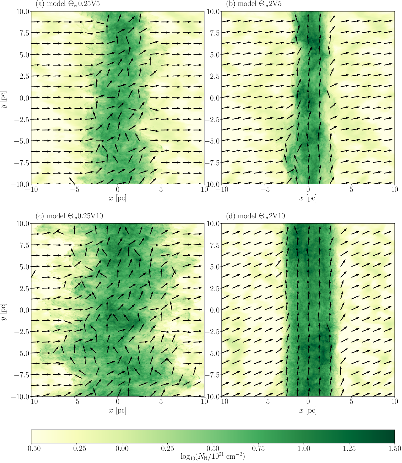
Figure 1: Column density maps integrated along the $z$-axis at $t=5~{}$Myr for models (a) $\Theta_{\mathrm{cr}}0.25\mathrm{V5}$, (b) $\Theta_{\mathrm{cr}}2\mathrm{V5}$, (c) $\Theta_{\mathrm{cr}}0.25\mathrm{V10}$, and (d) $\Theta_{\mathrm{cr}}2\mathrm{V10}$. The black arrows indicate the direction of the density-weighted mean magnetic field along the $z$-axis.

3.1 Global Properties of post-shock Layers

The early time evolution of the post-shock layers exhibits similar behaviors found in Paper I. Figure 1 shows the column densities integrated along the $z$-axis at $t=5$ Myr. The accretion of the CNM clumps through the shock fronts disturbs the post-shock layers significantly. For $\theta=0.25\theta_{\mathrm{cr}}$, the CNM clumps are not decelerated by the Lorentz force significantly after passing through the shock fronts because the compression is almost parallel to the magnetic field (Figures 1a and 1c). Figure 2a shows the time evolution of the mean (volume-averaged) kinetic, magnetic, and gravitational energy densities, ${E}_{\mathrm{kin}}$, ${E}_{\mathrm{mag}}$, ${E}_{\mathrm{grv}}$ of the post-shock layer for $\theta=0.25\theta_{\mathrm{cr}}$. We first focus on the results with $V_{0}=5~{}\mathrm{km~{}s^{-1}}$. The kinetic energies are always larger than the magnetic energies, indicating that the magnetic field lines are easily bent by the gas motion. This can be seen in the magnetic field directions that are random rather than organized as shown in Figures 1a and 1c.

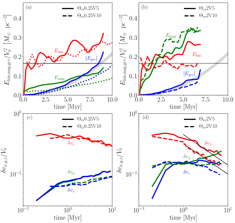
Figure 2: (Top panels) Time evolutions of (red) kinetic energy, (green) magnetic energy, and (blue) gravitational energy densities of the post-shock layers are compared between the models with (a) $\theta=0.25\theta_{\mathrm{cr}}$ and (b) $\theta=2\theta_{\mathrm{cr}}$. All the energy densities are divided by $V_{0}^{2}$. The gray line correspond to ${E}_{\mathrm{grv,ana}}$ shown in Equation (10). The horizontal black lines indicate the kinetic energy density flowing into the post-shock layer from the atomic gas, $\langle\rho_{0}\rangle V_{0}^{2}/2$. (Bottom panels) Time evolutions of the density-weighted velocity dispersions in the (red) $x$-, (green) $y$-, and (blue) $z$-directions for (c) $\theta=0.25\theta_{\mathrm{cr}}$ and (d) $\theta=2\theta_{\mathrm{cr}}$. In Panel (d), the two black lines correspond to the predictions from $\delta v_{x}/V_{0}=0.45\tau^{-1/2}$, where $\tau=t\left(\langle n_{0}\rangle/5~{}\mathrm{cm}^{-3}\right)\left(V_{0}/20~{}\mathrm{km~{}s^{-1}}\right)/(1~{}\mathrm{Myr})$ (Paper I) with $V_{0}=5~{}\mathrm{km~{}s^{-1}}$ and $10~{}\mathrm{km~{}s^{-1}}$. In all the panels, the solid and dashed lines show the results with $V_{0}=5~{}\mathrm{km~{}s^{-1}}$ and $10~{}\mathrm{km~{}s^{-1}}$, respectively.

An increase in $V_{0}$ from $5~{}\mathrm{km~{}s^{-1}}$ to $10~{}\mathrm{km~{}s^{-1}}$ does not change the physical properties of the post-shock layers for $\theta=0.25\theta_{\mathrm{cr}}$. Figure 2a clearly shows that all the energy densities are roughly proportional to $V_{0}^{2}$, keeping the relative ratios constant. This can be understood by the fact that the dynamics in the post-shock layers are driven by the ram pressure that is proportional to $V_{0}^{2}$.

Figure 2c shows that $\delta v_{x,y,z}/V_{0}$ does not depend on $V_{0}$ significantly, indicating that the velocity dispersions in the post-shock layers are proportional to the collision speed. For both the models, the degree of anisotropy of the velocity dispersion, which is defined as $\delta v_{x}/\sqrt{(\delta v_{y}^{2}+\delta v_{z}^{2})/2}$, is as large as $\sim 3$ for $V_{0}=5~{}\mathrm{km~{}s^{-1}}$ and $\sim 4$ for $V_{0}=10~{}\mathrm{km~{}s^{-1}}$ at $t=5$ Myr. In addition, $\delta v_{z}$ is almost identical to $\delta v_{y}$ for each model. This suggests that there is no preferential directions in the $(y,z)$-plane.

When $\theta$ is increased from $0.25\theta_{\mathrm{cr}}$ to $2\theta_{\mathrm{cr}}$ for $V_{0}=5~{}\mathrm{km~{}s^{-1}}$ (model $\Theta_{\mathrm{cr}}2\mathrm{V5}$), the physical properties of the post-shock layer drastically changes. Comparison between Figures 1a and 1b shows that the post-shock layer is thinner and denser for $\theta=2\theta_{\mathrm{cr}}$ because the Lorentz force owing to the shock-amplified magnetic field decelerates the CNM clumps efficiently for $\theta=2\theta_{\mathrm{cr}}$. The shock compression amplifies the magnetic energy that dominates over the kinetic energy at $t>2~{}$Myr (Figure 2b). Figure 1b shows that the magnetic field directions in the post-shock layer are parallel to the $y$-axis. At the early phase ($t<0.5~{}$Myr), Figures 2c and 2d show that $\delta v_{x}$ for model $\Theta_{\mathrm{cr}}2\mathrm{V5}$ is as large as that for model $\Theta_{\mathrm{cr}}0.25\mathrm{V5}$ because the magnetic field has not been amplified yet. In the subsequent evolution, $\delta v_{x}$ decreases in proportion to $t^{-1/2}$ (Paper I), and all the three components $\delta v_{x,y,z}$ become of similar magnitudes around $t\sim 5$ Myr.

Unlike model $\Theta_{\mathrm{cr}}0.25\mathrm{V5}$, there is anisotropy in the velocity dispersion in the $(y,z)$ plane for model $\Theta_{\mathrm{cr}}2\mathrm{V5}$. The velocity dispersion along the $y$-axis increases with time while $\delta v_{z}$ is constant with time. The continuous increase in $\delta v_{y}$ corresponds to the formation of filamentary structure by self-gravity, which will be shown in Figure 4.

Unlike the models with $\theta=0.25\theta_{\mathrm{cr}}$, the time evolution of the physical quantities depends on the collision speed for the $\theta=2\theta_{\mathrm{cr}}$ models. The relative importance of $E_{\mathrm{mag}}$ to the total energy is more significant for $V_{0}=10~{}\mathrm{km~{}s^{-1}}$ than for $V_{0}=5~{}\mathrm{km~{}s^{-1}}$. After the early evolution ($t<1~{}\mathrm{Myr}$) in which the velocity dispersions $\delta v_{x,y,z}$ increase in proportion to $V_{0}$, $\delta v_{x}$ begins to decrease earlier for $V_{0}=10~{}\mathrm{km~{}s^{-1}}$ than for $V_{0}=5~{}\mathrm{km~{}s^{-1}}$. This behavior is consistent with the results of Paper I where they found that $\delta v_{x}/V_{0}=0.3\tau^{-1/2}$, where $\tau=t\left(\langle n_{0}\rangle/5~{}\mathrm{cm}^{-3}\right)\left(V_{0}/20~{}\mathrm{km~{}s^{-1}}\right)/(1~{}\mathrm{Myr})$ The formula suggests that $\delta v_{x}/V_{0}$ is independent of $\langle\rho_{0}\rangle$ and $V_{0}$ if $\delta v_{x}$ is measured at the time of reaching the same column density. The effect of the rapid decrease in $\delta v_{x}$ can be seen in the fact that the shock fronts are flatter for $V_{0}=10~{}\mathrm{km~{}s^{-1}}$ (Figure 1b and 1d). The anisotropy of the velocity dispersions in the ($y,z$) plane exists also for the $V_{0}=10~{}\mathrm{km~{}s^{-1}}$. Interestingly, the epochs ($t\sim 5~{}\mathrm{Myr}$) when $\delta v_{x}$ becomes equal to $\delta v_{y}$ appear to be independent of $V_{0}$.

There are two main mechanisms to drive the post-shock turbulence. One is the accretion of the upstream CNN clumps as mentioned above. Since the momentum flux of the CNM clumps is much larger than the averaged post-shock momentum flux $\langle n_{0}\rangle V_{0}^{2}$, the accretion of the CNM clumps significantly disturbs the post-shock layers (Paper I). The other arises from deformation of the shock fronts that are generated by the interaction between the shock fronts and inhomogeneous upstream gas (Kobayashi et al., 2020). The post-shock velocity can be super-sonic if the shock normal is tilted more than $\sim 30$ degrees (Landau & Lifshitz, 1959).

The effect of the thermal instability on the post-shock turbulence is minor. Kobayashi et al. (2020) investigated how the post-shock turbulence depends on the amplitude of initial density perturbations. They found that the thermal instability contributes to drive turbulence only when $\delta n_{0}/\langle n_{0}\rangle$ is less than 10%, where $\delta n_{0}$ is the upstream density perturbation. In such situations, the energy conversion efficiency $\epsilon$ from the upstream kinetic energy $\langle\rho_{0}\rangle V_{0}^{2}/2$ to the post-shock turbulence energy is as low as a few percents. When $\delta n_{0}/n_{0}>10~{}\%$, the interaction between shock fronts and density inhomogeneity drives strong turbulence where $\epsilon$ is as high as 10%, which is roughly consistent with the values obtained in this paper, which is $\epsilon\sim(\delta v_{x}/V_{0})^{2}\sim 16\%$ (Paper I).

3.2 Structure Formation due to Self-gravity

Figures 2a and 2b show the time evolution of the gravitational energy densities of the post-shock layers that are estimated by

$$E_{\mathrm{grv}}=-\left(\int_{\mathrm{layer}}d^{3}x\right)^{-1}L^{2}\int_{\mathrm{layer}}\rho x\frac{\partial\phi}{\partial x}dx,$$ (9)

where the integration is done over the post-shock layer. The continuous accumulation of the atomic gas deepens the gravitational potential well, and $-E_{\mathrm{grv}}$ increases with time. The total energies of the post-shock layers however are positive, indicating that the post-shock layers remain unbound until at least the end of the simulations.

Assuming that the gas density is uniform inside the post-shock layer, one can derive the gravitational energy density analytically as follows:

$${E}_{\mathrm{grv,ana}}=-\frac{\pi G\Sigma_{0}(t)^{2}}{3},$$ (10)

where $\Sigma_{0}(t)=2\langle\rho_{0}\rangle V_{0}t$ is the mean column density of the post-shock layer. Figures 2a and 2b show that the time evolution of ${E}_{\mathrm{grv}}$ is consistent with that of ${E}_{\mathrm{grv,ana}}$ for all the models, indicating that the gravitational energy densities increase in proportion to $V_{0}^{2}$. The deviations of $E_{\mathrm{grv}}$ from $E_{\mathrm{grv,ana}}$ come from the non-uniform density distributions.

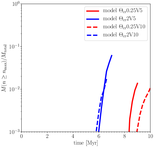
Figure 3: Time evolution of the mass fraction of dense gas with $n>n_{\mathrm{max}}$ for models (solid red) $\Theta_{\mathrm{cr}}0.25$V5, (solid blue) $\Theta_{\mathrm{cr}}2$V5, (dashed red) $\Theta_{\mathrm{cr}}0.25$V10, and (dashed blue) $\Theta_{\mathrm{cr}}2$V10.

As an indicator of star formation, we measure the mass fraction of the dense gas whose density is larger than $n_{\mathrm{max}}$ above which the cooling/heating processes are switched off to prevent gravitational collapse (Section 2.3).

The time evolution of the mass fraction of the dense gas with $n>n_{\mathrm{max}}$ does not depend on $V_{0}$ significantly for each $\theta$ (Figure 3). This behavior can be understood by the fact that the ratios of the thermal, kinetic, and magnetic energies to the gravitational energy are independent of $V_{0}$ (Figure 2). We expect that an increase of $\langle n_{0}\rangle$ accelerates the formation of the dense gas with $n>n_{\mathrm{max}}$ because the gravitational energy density is proportional to $\langle n_{0}\rangle^{2}$ while the ram pressure of the pre-shock gas is proportional to $\langle n_{0}\rangle$.

As is expected in Paper I, the formation of the dense gas with $n>n_{\mathrm{max}}$ is delayed by compressions with smaller $\theta$ because anisotropic super-Alfénic turbulence is driven for $\theta$ less than $\theta_{\mathrm{cr}}$.

Another interesting feature is that the difference in $V_{0}$ affects the formation of the dense gas with $n>n_{\mathrm{max}}$ in a different way at different $\theta$. As $V_{0}$ increases, the time evolution of the dense gas fraction does not change significantly for $\theta=2\theta_{\mathrm{cr}}$ while the formation of the dense gas is suppressed slightly for $\theta=0.25\theta_{\mathrm{cr}}$. This is due to the fact that the $\theta$-dependence of the velocity field differs depending on the collision velocity. For $\theta=0.25\theta_{\mathrm{cr}}$, the anisotropy of the velocity dispersion becomes more significant with increasing $V_{0}$ (Figure 2c).

We define $t_{\mathrm{first}}$, the time when the first bound clump is formed, as the earliest time at which the total energy of a clump with $n>n_{\mathrm{max}}$ becomes negative, where the clumps are identified by a friends-of-friends method. Table 1 lists $t_{\mathrm{first}}$, which are almost identical to the epochs when the mass with $n>n_{\mathrm{max}}$ increases rapidly as shown in Figure 3.

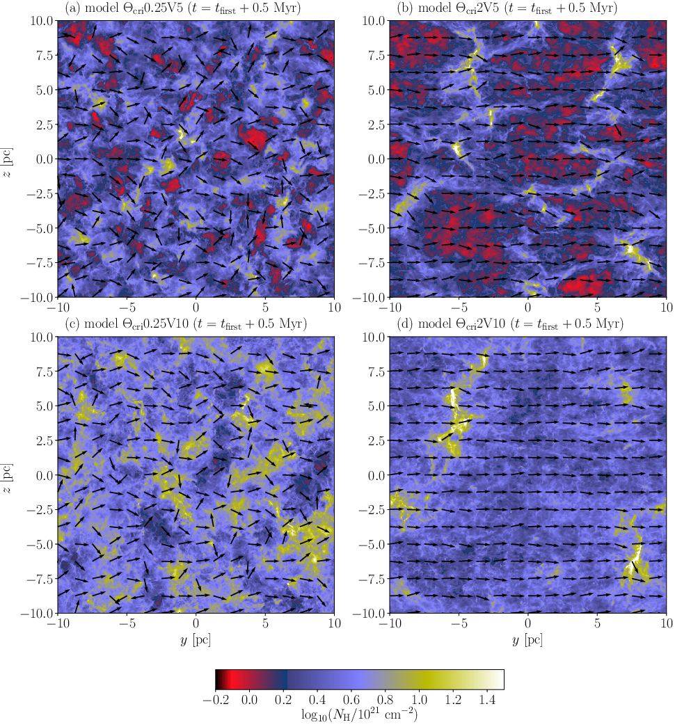
Figure 4: Color maps of the column densities integrated along the $x$-axis for models (a)$\mathrm{\Theta_{\mathrm{cr}}0.25V5}$, (b)$\mathrm{\Theta_{\mathrm{cr}}2V5}$, (c)$\mathrm{\Theta_{\mathrm{cr}}0.25V10}$, and (d)$\mathrm{\Theta_{\mathrm{cr}}2V10}$ at $t_{\mathrm{first}}+0.5~{}\mathrm{Myr}$. In each panel, the black arrows indicate the direction of the magnetic fields.

The column density distributions along the collision direction strongly depend on $\theta$ as shown in Figure 4. For the models with $\theta=2\theta_{\mathrm{cr}}$, prominent filamentary structures develop, and their elongations are roughly perpendicular to the mean magnetic field (Figures 4b and 4d). This is because the gas is accumulated by the self-gravity preferentially along with the magnetic fields. By contrast, the column density maps for the models with $\theta=0.25\theta_{\mathrm{cr}}$ do not show filamentary structures clearly. The projected magnetic fields are randomized. The detailed structure of filamentary clouds is investigated in forthcoming papers.

3.3 Field strength-density Relation

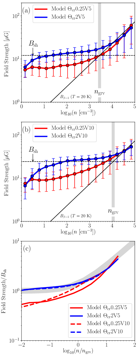
Figure 5: Mean field strength at each number density bin for the models with (a)$V_{0}=5~{}\mathrm{km~{}s^{-1}}$ and (b)$V_{0}=10~{}\mathrm{km~{}s^{-1}}$ at $t=t_{\mathrm{first}}+0.5$ Myr. Panels (a) and (b) compare the results with $\theta=0.25\theta_{\mathrm{cr}}$ and $2\theta_{\mathrm{cr}}$. The error bars correspond to the dispersion at a given density bin. The horizontal dashed lines indicate $B=B_{\mathrm{sh}}$. The field strength $B_{\beta=1}=\sqrt{8\pi\rho(0.3~{}\mathrm{km~{}s^{-1}})^{2}}$, which is proportional to $n^{1/2}$, is plotted in the black solid line. Panel (c) is the same as Panels (a) and (b) but the horizontal and vertical axes are normalized by $n_{\mathrm{grv}}$ and $B_{\mathrm{sh}}$, respectively. The thick gray line indicates the analytic formula shown in Equation (15).

The turbulence structures in the post-shock layers are reflected in the field strength-density ($B$-$n$) relation. Figures 5a and 5b show the mean field strengths as a function of density at $t_{\mathrm{first}}+0.5~{}\mathrm{Myr}$ for the models with $V_{0}=5~{}\mathrm{km~{}s^{-1}}$ and $V_{0}=10~{}\mathrm{km~{}s^{-1}}$, respectively.

We first consider the models with $V_{0}=5~{}\mathrm{km~{}s^{-1}}$ (Figure 5a). In low densities less than $10^{3}~{}\mathrm{cm}^{-3}$, model $\Theta_{\mathrm{cr}}2$V5 shows that the mean field strength is determined by the shock compression that amplifies the field strength up to

$$B_{\mathrm{sh}} = \sqrt{8\pi\langle\rho_{0}\rangle}V_{0}$$ (11)

$$= 12~{}\mu\mathrm{G}~{}\left(\frac{\langle n_{0}\rangle}{10~{}\mathrm{cm}^{-3}}\right)^{1/2}\left(\frac{V_{0}}{5~{}\mathrm{km~{}s^{-1}}}\right),$$

which is derived by balance between the pre-shock ram pressure and post-shock magnetic pressure. The independence of $B\sim B_{\mathrm{sh}}$ on $n$ for model $\Theta_{\mathrm{cr}}2$V5 reflects gas condensation along the magnetic field, corresponding to the formation of filaments. By contrast, for model $\Theta_{\mathrm{cr}}0.25$V5, the mean field strength ($\sim 6~{}\mu$G) is amplified by shear motion owing to the anisotropic super-Alfvénic turbulence. Assuming that the energy transfer efficiency from the kinetic energy to the magnetic energy $\epsilon$ is 20%, the following estimated field strength $B_{\mathrm{tur}}$ is consistent with the simulation results,

$$B_{\mathrm{tur}}=5.4~{}\mu\mathrm{G}\left(\frac{\epsilon}{0.2}\right)^{1/2}\left(\frac{\langle n_{0}\rangle}{10~{}\mathrm{cm}^{-3}}\right)^{1/2}\left(\frac{V_{0}}{5~{}\mathrm{km~{}s^{-1}}}\right).$$ (12)

Once the gas density becomes larger than $\sim 10^{3}~{}\mathrm{cm}^{-3}$, the $\theta$-dependence of the mean field strengths disappears, and the mean field strengths begin to increase with the gas density, following a similar $B$-$n$ relation. Interestingly, the mean field strengths in the high density range are consistent with the field strength $B_{\beta=1}$,

$$B_{\beta=1}=23~{}\mu\mathrm{G}~{}\left(\frac{c_{\mathrm{s}}}{0.3~{}\mathrm{km~{}s^{-1}}}\right)\left(\frac{n}{10^{4}~{}\mathrm{cm}^{-3}}\right)^{1/2},$$ (13)

which is given by $\beta=1$ at $T=20~{}$K that is a typical temperature of the dense regions, where $\beta$ is the plasma beta. This is where the self-gravity in the clumps becomes significant and the field amplification mode changes.

The $B$-$n$ relations of the models with $V_{0}=10~{}\mathrm{km~{}s^{-1}}$ behave similarly to those of the models with $V_{0}=5~{}\mathrm{km~{}s^{-1}}$. At each $\theta/\theta_{\mathrm{cr}}$, the field strength increases by a factor of two owing to the increase in $V_{0}$. This is consistent with the predictions from Equations (11) and (12). Similar to the models with $V_{0}=5~{}\mathrm{km~{}s^{-1}}$, in the high density regions, the field strengths follow $B_{\beta=1}$ although the density range is limited. The critical density where the transition between the low and high density regimes occurs is shifted toward high densities when $V_{0}$ increases from $5~{}\mathrm{km~{}s^{-1}}$ to $10~{}\mathrm{km~{}s^{-1}}$.

For the models with $\theta=2\theta_{\mathrm{cr}}$, the mean field strengths take a constant value of $B_{\mathrm{sh}}$ for lower densities and it increases following $B_{\beta=1}\propto n^{1/2}$ for higher densities (Figure 5b). From these facts, a critical density $n_{\mathrm{grv}}$ can be derived by equating $B_{\mathrm{sh}}$ and $B_{\beta=1}$ as follows:

$$n_{\mathrm{grv}} = \langle n_{0}\rangle\left(V_{0}/c_{\mathrm{s}}\right)^{2}$$ (14)

$$= 2.8\times 10^{3}~{}\mathrm{cm}^{-3}~{}\left(\frac{\langle n_{0}\rangle}{10~{}\mathrm{cm}^{-3}}\right)$$

$$\times\left(\frac{V_{0}}{5~{}\mathrm{km~{}s^{-1}}}\right)^{2}\left(\frac{c_{\mathrm{s}}}{0.3~{}\mathrm{km~{}s^{-1}}}\right)^{-2}.$$

When the density exceeds $n_{\mathrm{grv}}$, the self-gravitational force amplifies the magnetic fields.

Figure 5c is the same as Figures 5a and 5b but for the gas density and field strength are normalized by $n_{\mathrm{grv}}$ and $B_{\mathrm{sh}}$, respectively. The $B$-$n$ relation is characterized by $n_{\mathrm{grv}}$ and $B_{\mathrm{sh}}$ reasonably well for the models with $\theta=2\theta_{\mathrm{cr}}$. The mean field strength for the models is well approximated by

$$B_{\mathrm{ana}}=B_{\mathrm{sh}}\sqrt{1+\beta_{\mathrm{d}}^{-1}(n/n_{\mathrm{grv}})},$$ (15)

where $\beta_{\mathrm{d}}$ is a typical plasma $\beta$ for higher densities, and set to $1$ in Figure 5. Equation (15) is similar to that found by Tomisaka et al. (1988) who investigate the magnetohydrostatic structure of axisymmetric clouds.

4 Statistical Properties of Dense Clumps

In this section, we investigate the physical properties of dense clumps. The clumps are identified by connecting adjacent cells whose densities are larger than a threshold number density of $n_{\mathrm{th}}$. We extract dense clumps consisting of more than 100 cells, whose internal structure is sufficiently well resolved at least with 6 cells along the diameter. Dib et al. (2007) estimated errors for the terms in the virial theorem by using a uniform sphere, and found that the errors are not larger than $\sim 15~{}$% if the diameter of the sphere is resolved by four cells. Kobayashi et al. (2022) also found that the internal velocity dispersions of dense clumps are numerically converged if the clump size is resolved at least by 5 cells. This is because the largest scale of a clump, which corresponds to the clump size, has the largest power of the internal turbulence spectrum.

We choose a minimum threshold density of $10^{3}~{}\mathrm{cm}^{-3}$ because we could not identify dense clumps as an isolated structure at lower densities. We here consider the dense clumps identified with four different threshold densities ($n_{\mathrm{th}}=10^{3}~{}\mathrm{cm}^{-3}$, $10^{3.5}~{}\mathrm{cm}^{-3}$, $10^{4}~{}\mathrm{cm}^{-3}$, and $10^{4.5}~{}\mathrm{cm}^{-3}$). The spatial distributions of the dense clumps identified at $t=t_{\mathrm{first}}+0.5~{}\mathrm{Myr}$ are displayed in Figure 6. The filamentary structures seen in the left panels of Figures 4 correspond to the dense clumps with $n_{\mathrm{th}}\geq 10^{3.5}~{}\mathrm{cm}^{-3}$.

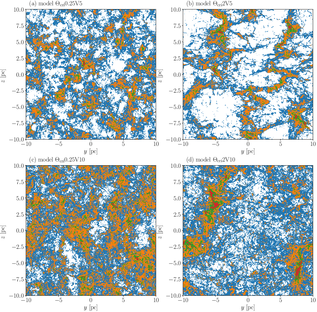
Figure 6: Spatial distributions of the dense clumps identified with four different threshold densities, $n_{\mathrm{th}}=$ (blue)$10^{3}~{}\mathrm{cm}^{-3}$, (orange)$10^{3.5}~{}\mathrm{cm}^{-3}$, (green)$10^{4}~{}\mathrm{cm}^{-3}$, and (red)$10^{4.5}~{}\mathrm{cm}^{-3}$ for models (a)$\Theta_{\mathrm{cr}}$0.25V5, (b)$\Theta_{\mathrm{cr}}$2V5, (c)$\Theta_{\mathrm{cr}}0.25$V10, and (d)$\Theta_{\mathrm{cr}}$2V10 at $t=t_{\mathrm{first}}+0.5~{}\mathrm{Myr}$.

We define the mass $M_{\mathrm{cl}}$, the position of the center of mass $\mathbf{x}_{\mathrm{cl}}$, and density-weighted mean velocity $\mathbf{v}_{\mathrm{cl}}$ of an identified clump as follows:

$$M_{\mathrm{cl}}=\int_{V}\rho d^{3}x,$$ (16)

$$\mathbf{\bf x}_{\mathrm{cl}}=\frac{1}{M_{\mathrm{cl}}}\int_{V}\rho\mathbf{x}d^{3}x,$$ (17)

$$\mathbf{\bf v}_{\mathrm{cl}}=\frac{1}{M_{\mathrm{cl}}}\int_{V}\rho\mathbf{v}d^{3}x,$$ (18)

where $V$ denotes the volume of each identified clump.

In this paper, when considering the virial theorem, the surface terms are neglected although they can be important to judge the stability of dense clumps (Dib et al., 2007). In a future paper, we will investigate the stability of dense clumps by taking into account the surface terms as well as the time evolution of filamentary structures.

The virial theorem without the surface terms is

$$\frac{1}{2}\frac{d^{2}I}{dt^{2}}=2\left({\cal E}_{\mathrm{th}}+{\cal E}_{\mathrm{kin}}\right)+{\cal E}_{\mathrm{mag}}+{\cal E}_{\mathrm{grv}}$$ (19)

where $I$ is the moment of inertia, ${\cal E}_{\mathrm{th}}$ and ${\cal E}_{\mathrm{kin}}$ are the thermal and kinetic energies

$${\cal E}_{\mathrm{th}}=\frac{3}{2}\int_{V}Pd^{3}x,\;\;\mathrm{and}\;\;{\cal E}_{\mathrm{kin}}=\frac{1}{2}\int_{V}\rho\mathbf{u}^{2}d^{3}x,$$ (20)

and ${\cal E}_{\mathrm{mag}}$ is the magnetic energy,

$${\cal E}_{\mathrm{mag}}=\int_{V}\frac{B^{2}}{8\pi}d^{3}x,$$ (21)

where $\mathbf{u}=(\mathbf{v}-\mathbf{v}_{\mathrm{cl}})$. In Equation (19), the gravitational energy is denoted by

$${\cal E}_{\mathrm{grv}}=-\int_{V}\rho\mathbf{r}\cdot\mathbf{\nabla}\phi d^{3}x,$$ (22)

where $\mathbf{r}=(\mathbf{x}-\mathbf{x}_{\mathrm{cl}})$. ${\cal E}_{\mathrm{grv}}$ is not exactly the same as the gravitational energy of the clump, and includes the tidal effect from the external gas. In this paper, ${\cal E}_{\mathrm{grv}}$ is called the gravitational energy. It can be positive when the tidal force exerted by the external gas destroys the clump.

In preparation for interpreting the results, we express the energies in terms of the mean values,

$${\cal E}_{\mathrm{th}}=\frac{3}{2}M_{\mathrm{cl}}c_{\mathrm{s}}^{2},$$ (23)

$${\cal E}_{\mathrm{kin}}=\frac{3}{2}M_{\mathrm{cl}}\delta u_{\mathrm{cl,1D}}^{2},$$ (24)

$${\cal E}_{\mathrm{mag}}=\frac{B_{\mathrm{cl}}^{2}}{8\pi}\frac{M_{\mathrm{cl}}}{\rho_{\mathrm{cl}}},$$ (25)

$${\cal E}_{\mathrm{grv}}\sim-\frac{3}{5}\frac{GM_{\mathrm{cl}}^{2}}{R_{\mathrm{cl}}}$$ (26)

where $c_{\mathrm{s}}$ is the mean sound speed, $\delta u_{\mathrm{cl,1D}}$ is the one-dimensional internal velocity dispersion, $B_{\mathrm{cl}}$ is the mean field strength, $V_{\mathrm{cl}}$ is the volume of dense clumps, $\rho_{\mathrm{cl}}=M_{\mathrm{cl}}/V_{\mathrm{cl}}$ is the mean density. In derivation of Equation (26), we assume a uniform spherical cloud with a radius of $R_{\mathrm{cl}}$. In this paper, as a size of clumps, we use

$$R_{\mathrm{cl}}=\left(\frac{3V_{\mathrm{cl}}}{4\pi\rho_{\mathrm{cl}}}\right)^{1/3}.$$ (27)

All the statistical quantities shown in this section are estimated using the dense clumps identified in $t_{\mathrm{first}}-0.5~{}\mathrm{Myr}\leq t\leq t_{\mathrm{first}}+0.5~{}\mathrm{Myr}$ to increase the number of samples.

4.1 The Virial Parameter

From the virial theorem without the surface terms (Equation (19)), a stability criterion can be derived by $\ddot{I}<0$, which is rewritten as

$$\alpha_{\mathrm{tot}}=\frac{2\left({\cal E}_{\mathrm{th}}+{\cal E}_{\mathrm{kin}}\right)+{\cal E}_{\mathrm{mag}}}{-{\cal E}_{\mathrm{grv}}}<1.$$ (28)

The virial parameter $\alpha_{\mathrm{tot}}$ is related to that often used in observations as a diagnose of the stability of dense clumps and cores (Bertoldi & McKee, 1992), but it contains the effect of support due to magnetic fields.

Before showing the dependence of $\alpha_{\mathrm{tot}}$ on $n_{\mathrm{th}}$, $M_{\mathrm{cl}}$, $V_{0}$, and $\theta$, we investigate the velocity structure of the dense clumps that are related to ${\cal E}_{\mathrm{kin}}$ in Sections 4.1.1 and 4.1.2.

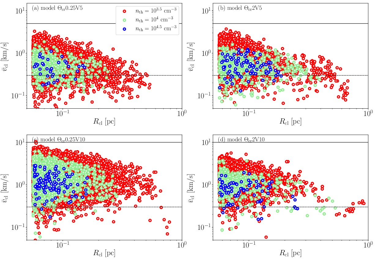
Figure 7: Bulk speeds as a function of the clump size $R_{\mathrm{cl}}$ at three different $n_{\mathrm{th}}$, (red) $10^{3.5}$, (green) $10^{4}$, and (blue) $10^{4.5}~{}\mathrm{cm}^{-3}$, for models (a)$\mathrm{\Theta_{\mathrm{cr}}0.25V5}$, (b)$\mathrm{\Theta_{\mathrm{cr}}2V5}$, (c)$\mathrm{\Theta_{\mathrm{cr}}0.25V10}$, and (d)$\mathrm{\Theta_{\mathrm{cr}}2V10}$. The horizontal solid and dashed lines correspond to the collision speed and sound speed in the dense regions, respectively.

4.1.1 Bulk Speeds

In Figure 2, we found that the velocity dispersions of the post-shock layers and their anisotropy in the post-shock layer depend not on $V_{0}$ significantly but on $\theta/\theta_{\mathrm{cr}}$. How are these velocity structures imprinted the motion and internal turbulence of the dense clumps?

Figures 7 show the bulk speeds of the clumps as a function of the clump size at three different threshold densities ($n_{\mathrm{th}}=10^{3.5}$, $10^{4}$, and $10^{4.5}~{}\mathrm{cm}^{-3}$). Figures 7a and 7b show that for all the models most clumps have supersonic bulk speeds because the sound speed is as low as $0.2-0.3~{}\mathrm{km~{}s^{-1}}$ (Koyama & Inutsuka, 2002). The bulk speeds decrease with the clump size on average although there are large dispersions.

In order to investigate how the bulk velocities of the dense clumps depend on $\theta$ in more detail, we measure the one-dimensional translational velocity dispersions of the bulk motion of the dense clumps with $R_{\mathrm{cl}}\leq 0.2~{}\mathrm{pc}$ that are defined as

$$\Delta v_{\mathrm{cl}}=\sqrt{\langle\left(\mathbf{v}_{\mathrm{cl}}-\langle\mathbf{v}_{\mathrm{cl}}\rangle\right)^{2}\rangle/3},$$ (29)

where the average is taken over all the dense clumps identified with each threshold density.

Figure 8a shows $\Delta v_{\mathrm{cl}}$ as a function of the mean clump density $\langle{n}_{\mathrm{cl}}\rangle$. All the model shows that $\Delta v_{\mathrm{cl}}$ decreases at a similar rate as $\langle{n}_{\mathrm{cl}}\rangle$ increases. The difference in $\theta$ does not have significant effect on $\Delta v_{\mathrm{cl}}$. By contrast, $\Delta v_{\mathrm{cl}}$ increases roughly in proportion to $V_{0}$. This comes from that the global velocity dispersions are in proportion to $V_{0}$, but are roughly independent of $\theta$ (Figures 2c and 2d). At $t=t_{\mathrm{first}}$, the global velocity dispersions are $\sim 1.7~{}\mathrm{km~{}s^{-1}}$ for both the models with $V_{0}=5~{}\mathrm{km~{}s^{-1}}$, are $\sim 3.4~{}\mathrm{km~{}s^{-1}}$ for model $\Theta_{\mathrm{cr}}0.25$V10 and $\sim 2.4~{}\mathrm{km~{}s^{-1}}$ for model $\Theta_{\mathrm{cr}}2$V10.

We further examine how the anisotropy of the velocity dispersions of the post-shock layers shown in Figure 2b carries over the anisotropy of ${\bf v}_{\mathrm{cl}}$. To characterize it, $f_{\mathrm{aniso}}\equiv\Delta v_{x,\mathrm{cl}}/\Delta v_{\perp,\mathrm{cl}}$ is defined as a representative value of the degree of anisotropy, where $\Delta v_{\perp,\mathrm{cl}}^{2}=(\Delta v_{y,\mathrm{cl}}^{2}+\Delta v_{z,\mathrm{cl}}^{2})/2$.

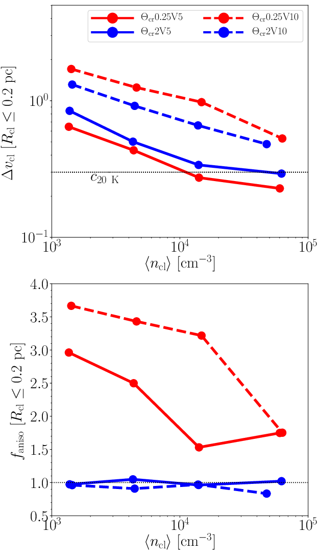
Figure 8: (a) Velocity dispersions of the bulk motion of the dense clumps with $R_{\mathrm{cl}}\leq 0.2~{}\mathrm{pc}$ for models (solid red)$\Theta_{\mathrm{cr}}0.25$V5, (solid blue)$\Theta_{\mathrm{cr}}2$V5, (dashed red)$\Theta_{\mathrm{cr}}0.25$V10, and (dashed blue)$\Theta_{\mathrm{cr}}2$V10 as a function of the mean clump density at four different threshold densities, $n_{\mathrm{th}}=10^{3},$ $10^{3.5}$, $10^{4}$, and $10^{4.5}~{}\mathrm{cm}^{-3}$. In each panel, the horizontal solid and dashed lines correspond to the collision speed and sound speed in the dense regions.

Figure 8b shows that unlike $\Delta v_{\mathrm{cl}}$, $f_{\mathrm{aniso}}$ depends more strongly on $\theta$ than on $V_{0}$. For both the models with $\theta=2\theta_{\mathrm{cr}}$, $f_{\mathrm{aniso}}$ is almost constant with ${n}_{\mathrm{cl}}$ and roughly equal to unity. This is consistent with Figure 2b. By contrast, the anisotropy in the models with $\theta=0.25\theta_{\mathrm{cr}}$ are more significant toward lower ${n}_{\mathrm{cl}}$. At $n_{\mathrm{th}}=10^{3}~{}\mathrm{cm}^{-3}$, $f_{\mathrm{iso}}$ is as high as $\sim 2.8$, which is consistent with $\delta v_{x}/\sqrt{(\delta v_{y}^{2}+\delta v_{z}^{2})/2}\sim 2.8$ for $V_{0}=5~{}\mathrm{km~{}s^{-1}}$ and $\sim 3.8$ for $V_{0}=10~{}\mathrm{km~{}s^{-1}}$ at $t=t_{\mathrm{first}}$ (Figure 2b).

For $\theta=0.25\theta_{\mathrm{cr}}$, the larger the collision speed, the higher $f_{\mathrm{aniso}}$ remains until the gas density becomes higher. This indicates that the ballistic motion of the dense clumps is maintained without much deceleration up to higher densities for larger $V_{0}$ (Figure 8).

4.1.2 Internal Velocity Dispersions

We here investigate the size-dependence of the internal velocity dispersion of each dense clump. The one-dimensional internal velocity dispersions of the clumps $\delta u_{\mathrm{cl,1D}}$ are plotted in Figures 9. They increase with the clump size in a power-law manner although the range of the clump sizes is small. We fit them using a power-law function of

$$\delta u_{\mathrm{cl,1D}}=\delta v_{0}\left(\frac{R_{\mathrm{cl}}}{1~{}\mathrm{pc}}\right)^{a}.$$ (30)

The best fit parameters are listed in Table 2. In the fitting, the clumps with $n_{\mathrm{th}}=10^{4.5}~{}\mathrm{cm}^{-3}$ are removed because a increase of $\delta u_{\mathrm{cl,1D}}$ due to self-gravity is found for $R_{\mathrm{cl}}>0.1~{}$pc in Figure 9.

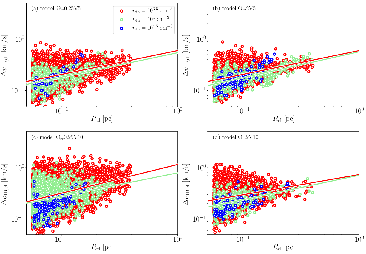
Figure 9: Internal velocity dispersions as a function of the clump size $R_{\mathrm{cl}}$ at three different $n_{\mathrm{th}}$, (red) $10^{3.5}$, (green) $10^{4}$, and (blue) $10^{4.5}~{}\mathrm{cm}^{-3}$, for models (a)$\Theta_{\mathrm{cr}}0.25$V5, (b)$\Theta_{\mathrm{cr}}2$V5, (c)$\Theta_{\mathrm{cr}}0.25$V10, and (d)$\Theta_{\mathrm{cr}}2$V10. In each panel, the two lines correspond to the lines of the best fit for (red) $10^{3.5}$, and (green) $10^{4}~{}\mathrm{cm}^{-3}$.

The power-law indices shown in Table 2 are consistent with $0.4-0.5$ for all the models, which is close to those of shock-dominated turbulence ($a=0.5$, Elsässer & Schamel, 1976) than incompressible Kolmogrov turbulence ($a=1/3$). They are consistent with observed values (e.g., Larson, 1981; Solomon et al., 1987).

$n_{\mathrm{th}}~{}[\mathrm{cm}^{-3}]$	$\Theta_{\mathrm{cr}}0.25$V5	$\Theta_{\mathrm{cr}}0.25$V10	$\Theta_{\mathrm{cr}}2$V5	$\Theta_{\mathrm{cr}}2$V10
$10^{3.5}$	$(0.60\pm 0.02)R_{\mathrm{1pc}}^{0.46\pm 0.01}$	$(1.15\pm 0.03)R_{\mathrm{1pc}}^{0.56\pm 0.01}$	$(0.57\pm 0.04)R_{\mathrm{1pc}}^{0.51\pm 0.03}$	$(0.73\pm 0.04)R_{\mathrm{1pc}}^{0.39\pm 0.02}$
$10^{4}$	$(0.54\pm 0.06)R_{\mathrm{1pc}}^{0.48\pm 0.05}$	$(0.79\pm 0.07)R_{\mathrm{1pc}}^{0.45\pm 0.03}$	$(0.57\pm 0.04)R_{\mathrm{1pc}}^{0.51\pm 0.03}$	$(0.71\pm 0.07)R_{\mathrm{1pc}}^{0.48\pm 0.04}$

Table 2: List of the best-fit formula of the internal velocity dispersions. From the second to fifth columns, the numbers in the parentheses represent $\delta v_{0}$ in $\mathrm{km~{}s^{-1}}$.

In order to investigate the parameter dependence of $\delta u_{\mathrm{cl,1D}}$ in more detail, we plot $\delta u_{\mathrm{cl,1D}}$ mass-weighted averaged over the clumps with $R_{\mathrm{cl}}\leq 0.2~{}$pc as a function of $\langle{n}_{\mathrm{cl}}\rangle$ in Figure 10. Like the bulk velocity dispersions $\langle\Delta v_{\mathrm{cl}}\rangle$, $\langle\delta u_{\mathrm{cl,1D}}\rangle$ depends more on $V_{0}$ than $\theta$. For $V_{0}=5~{}\mathrm{km~{}s^{-1}}$, the internal velocity dispersions are as low as $\sim 0.2-0.3~{}\mathrm{km~{}s^{-1}}$, regardless of ${n}_{\mathrm{cl}}$ for both $\theta=0.25\theta_{\mathrm{cr}}$ and $2\theta_{\mathrm{cr}}$. The internal velocity dispersions at $n_{\mathrm{th}}=10^{3}~{}\mathrm{cm}^{-3}$ increases roughly in proportion to $V_{0}$. Their scatters in $\delta u_{\mathrm{cl,1D}}$ also increase with $V_{0}$. Unlike for $V_{0}=5~{}\mathrm{km~{}s^{-1}}$, $\delta u_{\mathrm{cl,1D}}$ decreases with ${n}_{\mathrm{cl}}$ for $V_{0}=10~{}\mathrm{km~{}s^{-1}}$. As a result, the difference in $\delta u_{\mathrm{cl,1D}}$ between the models with different $V_{0}$ decreases as $\langle n_{\mathrm{cl}}\rangle$. This feature is consistent with the results of Audit & Hennebelle (2010).

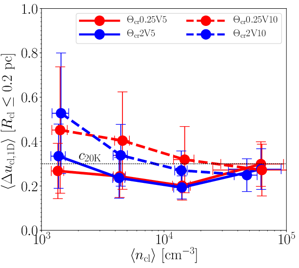
Figure 10: Mass-weighted average of the internal velocity dispersions as a function of the mean clump density at $n_{\mathrm{th}}=10^{3}$, $10^{3.5}$, $10^{4}$, and $10^{4.5}~{}\mathrm{cm}^{-3}$ for models (solid red)$\Theta_{\mathrm{cr}}0.25$V5, (solid blue)$\Theta_{\mathrm{cr}}2$V5, (dashed red)$\Theta_{\mathrm{cr}}0.25$V10, and (dashed blue)$\Theta_{\mathrm{cr}}$2V10. The average is performed over the dense clumps with $R_{\mathrm{cl}}<0.2$ pc. The horizontal and vertical error bars indicate the dispersions of the mean density and internal velocity dispersion at each threshold density, respectively.

4.1.3 Virial Parameters

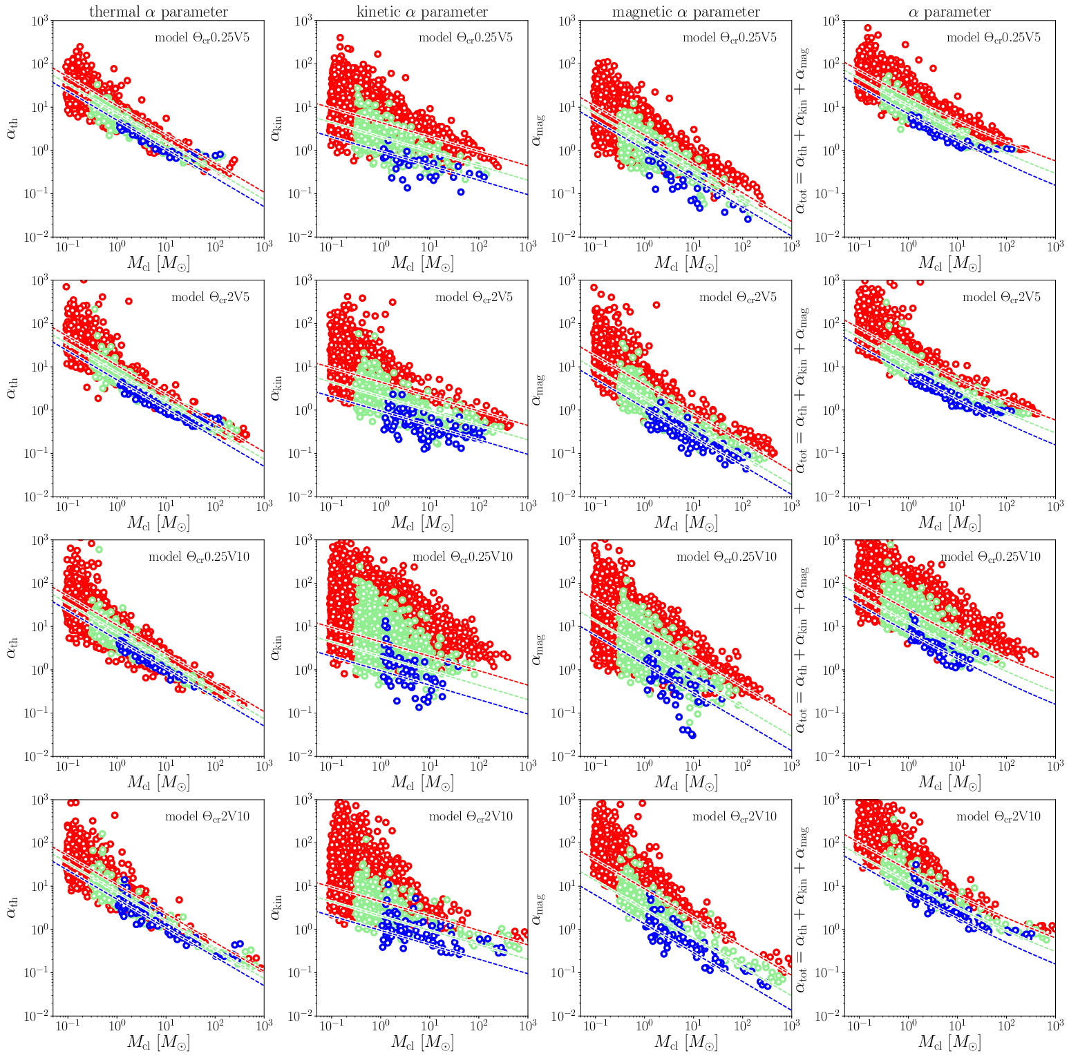
Figure 11: (first column) Thermal, (second column) kinetic, and (third column) magnetic virial parameters as a function of the clump mass at (red) $n_{\mathrm{th}}=10^{3.5}$, (green) $10^{4}$, and (blue) $10^{4.5}~{}\mathrm{cm}^{-3}$ for models (first row) $\Theta_{\mathrm{cr}}0.25$V5, (second row) $\Theta 2$V5, (third row) $\Theta_{\mathrm{cr}}0.25$V10, and (forth row) $\Theta_{\mathrm{cr}}2$V10. The forth column shows the total virial parameter $\alpha_{\mathrm{tot}}=\alpha_{\mathrm{th}}+\alpha_{\mathrm{kin}}+\alpha_{\mathrm{mag}}$. In each panel, the three dashed lines correspond to the predictions from the analytic formula (Equations (32), (34), (36), and (37)).

The virial parameter (Equation (28)) is divided into three contributions, thermal, kinetic, and magnetic virial parameters as follows:

$$\alpha_{\mathrm{th}}=\frac{2{\cal E}_{\mathrm{th}}}{-{\cal E}_{\mathrm{grv}}},\;\;\alpha_{\mathrm{kin}}=\frac{2{\cal E}_{\mathrm{kin}}}{-{\cal E}_{\mathrm{grv}}},\;\;\mathrm{and}\;\;\alpha_{\mathrm{mag}}=\frac{{\cal E}_{\mathrm{mag}}}{-{\cal E}_{\mathrm{grv}}}.\;\;$$ (31)

Figure 11 illustrates the three virial parameters ($\alpha_{\mathrm{th}}$, $\alpha_{\mathrm{kin}}$, and $\alpha_{\mathrm{mag}}$) as a function of the clump mass at three density thresholds. One can see that the three virial parameters have different $M_{\mathrm{cl}}$ and $n_{\mathrm{th}}$-dependence. Focusing on the $M_{\mathrm{cl}}$-dependence, as $M_{\mathrm{cl}}$ increases, $\alpha_{\mathrm{th}}$ and $\alpha_{\mathrm{mag}}$ both decrease at a rate of $\propto M_{\mathrm{cl}}^{-0.6}$ while $\alpha_{\mathrm{kin}}$ decreases more slowly following $\propto M_{\mathrm{cl}}^{-0.3}$. All the virial parameters decrease with $n_{\mathrm{th}}$, keeping their trend unchanged while the decreasing rate depends on $\theta$ and $V_{0}$.

In order to explain the simulation results, we here derive analytic formula of $\alpha_{\mathrm{th}}$, $\alpha_{\mathrm{kin}}$, and $\alpha_{\mathrm{mag}}$. First we consider the thermal virial parameter. Using Equations (23) and (26), Equation (31) is rewritten as

$$\alpha_{\mathrm{th,ana}}\sim\frac{5R_{\mathrm{cl}}}{GM_{\mathrm{cl}}}c_{\mathrm{s}}^{2}=9c_{0.3}^{2}\rho_{4}^{-1/3}M_{1}^{-2/3},$$ (32)

where $c_{0.3}=c_{\mathrm{s}}/0.3~{}\mathrm{km~{}s^{-1}}$, $\rho_{4}=\rho_{\mathrm{cl}}/(10^{4}\mu m_{\mathrm{H}}~{}\mathrm{cm}^{-3})$, and $M_{1}=M_{\mathrm{cl}}/1~{}M_{\odot}$. Equation (32) is essentially the same as that derived by Bertoldi & McKee (1992) and Lada et al. (2008). The thermal virial parameters are consistent with the predictions from Equations (32) for all the models (the first column of Figure 11).

The kinetic virial parameter is estimated as

$$\alpha_{\mathrm{kin,ana}}\sim\frac{5R_{\mathrm{cl}}}{GM_{\mathrm{cl}}}\delta u_{\mathrm{cl,1D}}^{2}=\frac{5R_{\mathrm{cl}}}{GM_{\mathrm{cl}}}\delta v_{0}^{2}\left(\frac{R_{\mathrm{cl}}}{R_{0}}\right),$$ (33)

where the internal velocity dispersion $\delta u_{\mathrm{cl,1D}}=\delta u_{0}\left(R_{\mathrm{cl}}/R_{0}\right)^{0.5}$ is used (Section 4.1.2). Equation (33) becomes

$$\alpha_{\mathrm{kin,ana}}\sim 9\delta u_{1}^{2}\rho_{4}^{-2/3}M_{1}^{-1/3}$$ (34)

where we use $\delta u_{1}=\delta u_{0}/1~{}\mathrm{km~{}s^{-1}}$ and $R_{0}=1~{}\mathrm{pc}$ for all the models because $\delta u_{\mathrm{cl,1D}}$ roughly converges to $\sim 0.6~{}\mathrm{km~{}s^{-1}}~{}(R_{\mathrm{cl}}/1~{}\mathrm{pc})^{0.5}$ toward higher clump densities, regardless of the parameters $V_{0}$ and $\theta$ (Section 4.1.2). The mass-dependence of $\alpha_{\mathrm{kin}}$ is weaker than that of $\alpha_{\mathrm{th}}$, indicating that $\alpha_{\mathrm{kin}}$ dominates over $\alpha_{\mathrm{th}}$ for more massive clumps. Comparison between $\alpha_{\mathrm{kin}}$ and the predictions from Equation (34) shows that Equation (34) reproduces the simulation results reasonably well in higher densities although deviations are found in lower clump densities for $V_{0}=10~{}\mathrm{km~{}s^{-1}}$ as expected.

The magnetic virial parameter is expressed as

$$\alpha_{\mathrm{mag,ana}}\sim\frac{B_{\mathrm{cl}}^{2}}{8\pi\rho_{\mathrm{cl}}}\frac{5R_{\mathrm{cl}}}{3GM_{\mathrm{cl}}}.$$ (35)

The field strength $B_{\mathrm{cl}}$ is estimated from the $B$-$n$ relation shown in Figure 5. For the models with $\theta=2\theta_{\mathrm{cr}}$, the density-dependence of the field strength is characterized by $n_{\mathrm{grv}}$. Substituting Equation (15) into Equation (35) one obtains

$$\alpha_{\mathrm{mag,ana}}\sim 3c_{0.3}^{2}\rho_{4}^{-1/3}M_{1}^{-2/3}\left(\beta_{\mathrm{d}}^{-1}+\frac{n_{\mathrm{grv}}}{{n}_{\mathrm{cl}}}\right).$$ (36)

This equation shows that the magnetic virial parameter decreases in proportion to $M_{1}^{-2/3}$. This dependence is the same as that of $\alpha_{\mathrm{th}}$ as shown in Figure 11. The predictions from Equation (36) are consistent with the simulation results (the third column of Figure 11).

Note that $\alpha_{\mathrm{mag}}$ is closely related with the mass-to-flux ratio that is estimated observationally by the Zeemann measurement (Crutcher, 1999; Heiles & Troland, 2005; Crutcher et al., 2010). We will discuss an asymptotic property of the mass-to-flux ratio of dense clumps in Section 5.1.

Combining Equation (32), (34), and (36), one obtains the analytic expression of the total $\alpha$ parameter,

$$\alpha_{\mathrm{tot,ana}} = \left(9+3\beta_{\mathrm{d}}^{-1}+3\frac{n_{\mathrm{grv}}}{{n}_{\mathrm{cl}}}\right)c_{0.3}^{2}\rho_{4}^{-1/3}M_{1}^{-2/3}$$ (37)

$$+ 9\delta v_{1}^{2}\rho_{4}^{-2/3}M_{1}^{-1/3},$$

where the first term in the right-hand side corresponds to $\alpha_{\mathrm{th}}+\alpha_{\mathrm{mag}}$ and the remaining term corresponds to $\alpha_{\mathrm{kin}}$.

It is worth noting the importance of the magnetic support in $\alpha_{\mathrm{tot,ana}}$ (Equation (37)). For clumps with $\rho_{\mathrm{cl}}>\rho_{\mathrm{grv}}$, the field strength is roughly determined by the condition $\beta\sim O(1)$. The third term in the parentheses of the first term in the right-hand side of Equation (37) is negligible compared with the other two terms. In such a dense clump, the magnetic field is only of secondary importance in $\alpha_{\mathrm{tot,ana}}$ because $\alpha_{\mathrm{th,ana}}$ is three times larger than $\alpha_{\mathrm{mag,ana}}$ when $\beta_{\mathrm{d}}=1$ ($\alpha_{\mathrm{th}}/\alpha_{\mathrm{mag}}=2{\cal E}_{\mathrm{th}}/{\cal E}_{\mathrm{mag}}\sim 3\beta$). This finding suggests that the masses of clumps and cores are determined almost independently of the magnetic field strength once $\rho_{\mathrm{cl}}$ exceeds $\rho_{\mathrm{grv}}$.

The diffuse clumps with

$${n}_{\mathrm{cl}}<\frac{n_{\mathrm{grv}}}{3} = 10^{3}~{}\mathrm{cm}^{-3}\left(\frac{\langle n_{0}\rangle}{10~{}\mathrm{cm}^{-3}}\right)$$ (38)

$$\left(\frac{V_{0}}{5~{}\mathrm{km~{}s^{-1}}}\right)^{2}\left(\frac{c_{\mathrm{s}}}{0.3~{}\mathrm{km~{}s^{-1}}}\right)^{-2}$$

are expected to be mainly supported by the shock-amplified magnetic fields if the contribution of the kinetic energy is excluded. This is because the third term dominates over the other two terms in the parentheses of the first term in the right-hand side of Equation (37). In our setup, the condition is met when ${n}_{\mathrm{cl}}<10^{3}~{}\mathrm{cm}^{-3}$ for $V_{0}=5~{}\mathrm{km~{}s^{-1}}$ and ${n}_{\mathrm{cl}}<4\times 10^{3}~{}\mathrm{cm}^{-3}$ for $V_{0}=10~{}\mathrm{km~{}s^{-1}}$. This is why magnetically-supported dense clumps with $n_{\mathrm{th}}\geq 10^{4}~{}\mathrm{cm}^{-3}$ are not seen in our results.

5 Discussions

5.1 Mass-to-Flux Ratio

The mass-to-flux ratio $\mu$ is often used to evaluate the importance of magnetic fields in cloud stability. If the mass-to-flux ratio is larger than the critical value of $\mu_{\mathrm{cr}}=1/2\pi\sqrt{G}$, magnetic fields are not strong enough to support clumps against self-gravity A factor of $1/2\pi$ slightly changes depending on the clump shape (Strittmatter, 1966; Mouschovias & Spitzer, 1976; Nakano & Nakamura, 1978; Tomisaka et al., 1988; Tomisaka, 2014). Observationally $\mu$ is often estimated by taking the ratio between the column density and the field strength measured by the Zeeman effect (Crutcher, 1999; Heiles & Troland, 2005; Crutcher et al., 2010).

In terms of $\alpha_{\mathrm{mag}}$, the mass-to-flux ratio is expressed as

$$\frac{\mu}{\mu_{\mathrm{cr}}}\sim\left(\alpha_{\mathrm{mag}}\right)^{-1/2}=\left(\frac{{\cal E}_{\mathrm{mag}}}{-{\cal E}_{\mathrm{grv}}}\right)^{-1/2}.$$ (39)

From Equation (36), $\mu/\mu_{\mathrm{cr}}$ is expected to be proportional to $M_{\mathrm{cl}}^{1/3}$, regardless of $\theta$. This mass dependence was confirmed in the third column of Figure 11. In simulations of cloud-cloud collision, Sakre et al. (2021) found that as the clump mass increases, the magnetic energy increases more slowly than the gravitational energy, which is consistent with the positive $M_{\mathrm{cl}}$ dependence of the mass-to-flux ratio. Considering compressions along the magnetic field, Banerjee et al. (2009) and Inoue & Inutsuka (2012) found a similar mass-dependence of the mass-to-flux ratios which follow $\propto M_{\mathrm{cl}}^{0.4}$. Iffrig & Hennebelle (2017) also found a similar relation in semi-global galactic-disk simulations, and explained the mass-dependence by a similar argument as in this paper.

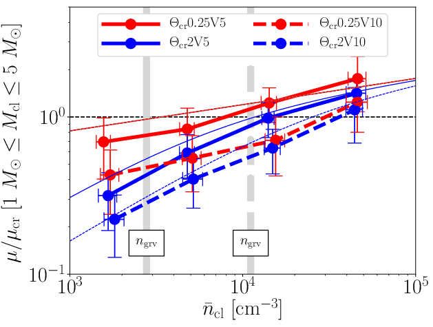
Figure 12: Mass-to-flux ratios averaged over the clumps with $1~{}M_{\odot}\leq M_{\mathrm{cl}}\leq 5~{}M_{\odot}$ as a function of the clump mean density for models (solid red)$\Theta_{\mathrm{cr}}0.25$V5, (solid blue)$\Theta_{\mathrm{cr}}2$V5, (dashed red)$\Theta_{\mathrm{cr}}0.25$V10, and (dashed blue)$\Theta_{\mathrm{cr}}$2V10. The vertical solid and dashed gray lines indicate $n_{\mathrm{grv}}$ with $V_{0}=5~{}\mathrm{km~{}s^{-1}}$ and $10~{}\mathrm{km~{}s^{-1}}$, respectively. The thin red line corresponds to the mass-to-flux ratios assuming $\beta=1$. The thin solid and dashed blue lines indicate the predictions from Equation (36) with $M_{\mathrm{cl}}=3~{}M_{\odot}$ for $V_{0}=5~{}\mathrm{km~{}s^{-1}}$ and $V_{0}=10~{}\mathrm{km~{}s^{-1}}$, respectively.

We plot the mass-to-flux ratios averaged over $1~{}M_{\odot}\leq M_{\mathrm{cl}}\leq 5~{}M_{\odot}$ as a function of the mean clump density in Figure 12. The $\theta=2\theta_{\mathrm{cr}}$ models show that the mass-to-flux ratios are consistent with the predictions from the analytic formula (Equation (36)). Equation (36) predicts

$$\frac{\mu_{\beta}}{\mu_{\mathrm{cr}}}=0.6\beta_{\mathrm{d}}^{1/2}c_{0.3}^{-1}\rho_{4}^{1/6}M_{1}^{1/3}$$ (40)

for ${n}_{\mathrm{cl}}>n_{\mathrm{grv}}$ and

$$\frac{\mu_{\mathrm{sh}}}{\mu_{\mathrm{cr}}}=1.1\langle\rho_{0}\rangle_{1}^{-1/2}V_{5}^{-1}\rho_{4}^{2/3}M_{1}^{1/3}$$ (41)

for ${n}_{\mathrm{cl}}<n_{\mathrm{grv}}$. The mass-to-flux ratios increase in proportion to ${n}_{\mathrm{cl}}^{2/3}$ until ${n}_{\mathrm{cl}}$ reaches $n_{\mathrm{grv}}$. When ${n}_{\mathrm{cl}}$ exceeds $n_{\mathrm{grv}}$, the mass-to-flux ratios approach the asymptotic line given by the condition $\beta\sim 1$. The difference in $V_{0}$ appears in how fast $\mu$ approaches $\mu_{\beta}$.

The difference in $\mu/\mu_{\mathrm{cr}}$ between the models disappear when ${n}_{\mathrm{cl}}$ exceeds $n_{\mathrm{grv}}$ because the field strength is determined by the condition $\beta\sim O(1)$ (Figure 5). Comparison between the simulation results and the predictions from Equation (36) with $M_{\mathrm{cl}}=3~{}M_{\odot}$ shows that they are consistent for both the models.

For ${n}_{\mathrm{cl}}>n_{\mathrm{grv}}$, the mass-to-flux ratios are insensitive to ${n}_{\mathrm{cl}}$ (Figure 12) since $\mu_{\beta}\propto{n}_{\mathrm{cl}}^{1/6}.$ This means that the mass-to-flux ratio does not change significantly once ${n}_{\mathrm{cl}}$ becomes larger than $n_{\mathrm{grv}}$. We thus define the characteristic mass-to-flux ratio $\mu_{\mathrm{ch}}$ for which ${n}_{\mathrm{cl}}$ is equal to $n_{\mathrm{grv}}$,

$$\frac{\mu_{\mathrm{ch}}}{\mu_{\mathrm{cr}}}=0.5\beta_{\mathrm{d}}^{1/2}c_{0.3}^{-4/3}\langle\rho_{0}\rangle_{1}^{1/6}V_{5}^{1/3}M_{1}^{1/3}.$$ (42)

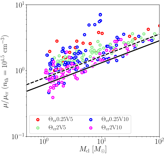
Figure 13: Mass-to-flux ratios of the dense clumps with $n_{\mathrm{th}}=10^{4.5}~{}\mathrm{cm}^{-3}$ as a function of the clump mass for models (red)$\Theta_{\mathrm{cr}}0.25$V5, (green)$\Theta_{\mathrm{cr}}2$V5, (blue)$\Theta_{\mathrm{cr}}0.25$V10, and (magenta)$\Theta_{\mathrm{cr}}$2V10. The solid and dashed lines correspond to $\mu_{\mathrm{ch}}/\mu_{\mathrm{cr}}$ with $V_{0}=5~{}\mathrm{km~{}s^{-1}}$ and $V_{0}=10~{}\mathrm{km~{}s^{-1}}$, respectively.

Figure 13 shows the mass-to-flux ratios of the dense clumps with $n_{\mathrm{th}}=10^{4.5}~{}\mathrm{cm}^{-3}$, which are almost independent of the parameters $V_{0}$ and $\theta$. This is consistent with what we found in Figure 12. We compare the mass-to-flux ratios of the dense clumps with $n_{\mathrm{th}}=10^{4.5}~{}\mathrm{cm}^{-3}$ with the predictions from Equation (42) in Figure 12. One can see that they are consistent. The reason why the measured mass-to-flux ratios are slightly larger than the predictions is that the clump density is larger than $n_{\mathrm{grv}}$.

Interestingly, $\mu_{\mathrm{ch}}/\mu_{\mathrm{cr}}$ is roughly equal to unity, and it is insensitive to the collision parameters $(\langle n_{0}\rangle,V_{0})$. The sound speed is expected to decrease to 0.2 $\mathrm{km~{}s^{-1}}$ when the gas density increases further, $\mu_{\mathrm{ch}}/\mu_{\mathrm{cr}}$ increases by a factor of two (Equation (42)). We thus expect that dense clumps with $\sim 1~{}M_{\odot}$ become super-critical if their mean densities exceed $n_{\mathrm{grv}}$ in a wide range of the collision parameters.

5.2 Internal Alfén Mach number

We here show the ratio between the kinetic energy and magnetic energy, or Alfvén mach number,

$${\cal M}_{\mathrm{A}}=\sqrt{{{\cal E}_{\mathrm{kin}}}/{{\cal E}_{\mathrm{mag}}}}.$$ (43)

Using Equations (15) and (30), one obtains the following analytic formula,

$${\cal M}_{\mathrm{A,\beta}}=1.2\delta u_{1}c_{0.3}^{-1}\rho_{4}^{-1/6}M_{1}^{1/6}$$ (44)

for $n>n_{\mathrm{grv}}$, and

$${\cal M}_{\mathrm{A,sh}}=2.3\delta u_{1}V_{5}^{-1}\langle\rho_{0}\rangle_{1}^{-1/2}\rho_{4}^{1/3}M_{1}^{1/6}$$ (45)

for $n<n_{\mathrm{grv}}$. If the ram pressure of the colliding flow $\langle\rho_{0}\rangle V_{0}^{2}$ is extremely large, the Alfvén Mach number can be small in the low density regions with $n<n_{\mathrm{grv}}$. Once the number density exceeds $n_{\mathrm{grv}}$, Equation (44) shows that the Alfvén Mach number converges to order of unity. This result is robust because it is extremely insensitive to both the clump density and mass. This feature is consistent with observations by Myers & Goodman (1988) and Crutcher (1999).

5.3 Structures of Filamentary Clouds

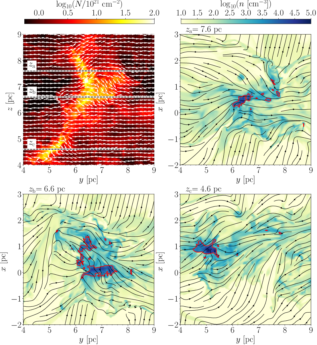
Figure 14: The top-left panel shows the column density map in $4~{}\mathrm{pc}\leq y,z\leq 9~{}\mathrm{pc}$ for model $\Theta_{\mathrm{cr}}2\mathrm{V}5$. The white arrows indicate the directions of the projected magnetic fields density-weighted-averaged along the $x$-axis. The remaining three panels correspond to the density slices at $z=z_{\mathrm{a}}=7.6~{}$pc, $z_{\mathrm{b}}=6.6$ pc, and $z_{\mathrm{c}}=4.6$ pc. The red lines indicate the contours of $n=10^{3.5}~{}\mathrm{cm}^{-3}$. The black lines show the stream lines of the vector field $(B_{y},B_{x})$.

In our models, prominent filamentary structures form only for $\theta>\theta_{\mathrm{cr}}$ (Figure 4) because super-Alfvénic turbulence prevents such a coherent structure from forming for $\theta<\theta_{\mathrm{cr}}$. Our results are consistent with the observational results (e.g., André et al., 2010) because compressions with $\theta<\theta_{\mathrm{cr}}$ is extremely rare if compressions are isotropic (Paper I). In reality, the magnetic fields are not uniform but have different orientations, depending on the location. Compressions with $\theta<\theta_{\mathrm{cr}}$ are unlikely to occur over a wide area.

In this section, the internal structures of the filaments are briefly shown for model $\Theta_{\mathrm{cr}}$2V5 although they will be investigated in detail in forthcoming papers. We extract one of the filaments from the simulation results and its column density is shown in the top-left panel of Figure 14. Overall, the projected magnetic fields are perpendicular to the filament, which is consistent with observational results (e.g., Alves et al., 2008; Sugitani et al., 2010; Chapman et al., 2011).

The three dimensional structure of filaments is not a cylinder but more like a “ribbon”. The top-right and bottom panels of Figure 14 correspond to the density slices at $z=z_{\mathrm{a}}$, $z_{\mathrm{b}}$, and $z_{\mathrm{c}}$, whose positions are shown in the top-left panel of Figure 14. The cross sections of the filament are flattened along the local magnetic field direction. Ribbon-like flattened structures are a natural configuration of strongly-magnetized filaments because the anisotropic nature of the Lorentz force, whose direction is perpendicular to the local magnetic field (Tomisaka, 2014; Auddy et al., 2016).

Interestingly, the elongated direction of the flattened density structures varies significantly along the filament axis because the directions of the magnetic fields significantly vary as shown in the density-slice plots of Figure 14. For instance, at $z=z_{\mathrm{b}}$, the minor axis of the flattened structure found around $(y,x)\sim(7~{}\mathrm{pc},0~{}\mathrm{pc})$ is parallel to the line-of-sight direction (the $x$-axis). That is why the widths of the filament around $z=z_{\mathrm{b}}$ appear to be larger than those of the other regions (the top panel of Figure 14).

5.4 A Universal $B$-$n$ Relation

The $B$-$n$ relation for high densities reflects how the magnetic field is amplified during gas contraction. The gravitational collapse of a spherical cloud with extremely weak magnetic fields leads to the scaling law $B\propto n^{2/3}$ (Mestel, 1965). By contrast, a cloud flattened by the existence of the magnetic field undergoes gravitational contraction with $B\propto n^{1/2}$, indicating that the plasma beta remains constant (Mouschovias, 1976; Tomisaka et al., 1988).

Our analytic formulae derived in Section 4 rely on the speculation that the field strength is determined by a condition of $\beta\sim O(1)$ in the high density limit, regardless of $\theta$.

We first present a simple argument of why the central plasma $\beta$ of gravitationally contracting flattened clouds should be $O(1)$. We then compare the $B$-$n$ relations of our work with those of the previous studies in Section 5.4.2, and those inferred from observational studies in Section 5.4.3.

5.4.1 $B$-$n$ Relations of Gravitationally Contracting Flattened Clouds

In Section 5.3, we found that the dense clumps have ribbon-like structures flattened along the local magnetic field for model $\Theta_{\mathrm{cr}}2$V5. Also for the other filaments of models $\Theta_{\mathrm{cr}}2$V5 and $\Theta_{\mathrm{cr}}2$V10, similar ribbon-like structures are found. Thus, at least for $\theta=2\theta_{\mathrm{cr}}$, the dense clumps form through gas accumulation along the magnetic fields.

We here investigate how magnetic fields are amplified by self-gravity using a simple ribbon model. As shown in Figure 15, a flattened ribbon-like filament with the central density $\rho_{\mathrm{c}}$, the line mass $M_{\mathrm{L}}$, and the width $d_{0}$ is considered. The uniform magnetic field, whose strength is $B_{0}$, is perpendicular to the ribbon surface. The thickness of the ribbon is determined by the thermal Jeans length,

$$h=\frac{c_{\mathrm{s}}}{\sqrt{2\pi G\rho_{\mathrm{c}}}}.$$ (46)

The relation between $\rho_{\mathrm{c}}$ and column density $\Sigma=M_{\mathrm{L}}/d_{0}$ is

$$\rho_{\mathrm{c}}=\frac{\pi G\Sigma^{2}}{2c_{\mathrm{s}}^{2}}.$$ (47)

The flux-freezing condition gives

$$Bd_{0}=\frac{B}{\Sigma}\times M_{\mathrm{L}}=\mathrm{const.}$$ (48)

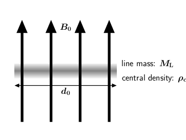
Figure 15: Schematic picture of the ribbon with the width $d_{0}$ and line mass $M_{\mathrm{L}}$. The ribbon extends in the direction parallel to the sheet. The central density is assumed to be $\rho_{\mathrm{c}}$, and the density is assumed to be independent of the width. The uniform magnetic field (field strength $B_{0}$) is parallel to the minor axis of the ribbon.

We here consider the situation that the ribbon grows by gas accretion along the magnetic field. Initially, the disk is not massive enough to contract radially due to the magnetic pressure. In order for the disk to contract radially, the mass-to-flux ratio be larger than the critical value,

$$\frac{\Sigma}{B_{0}}>\frac{1}{2\pi\sqrt{G}}$$ (49)

(Nakano & Nakamura, 1978). From this, we define a critical column density of

$$\Sigma_{\mathrm{cr}}=\frac{B_{0}}{2\pi\sqrt{G}}.$$ (50)

Once the column density of the ribbon reaches this critical value, the ribbon begins to contract radially. The line mass at this epoch is denoted by $M_{\mathrm{L,cr}}$,

$$M_{\mathrm{L,cr}}=\frac{d_{0}B_{0}}{2\pi\sqrt{G}}.$$ (51)

This is essentially the same as the critical line mass at the large magnetic flux limit derived by Tomisaka (2014).

Using Equation (47) and (48) ($M_{\mathrm{L}}\Sigma/B=M_{\mathrm{L,cr}}\Sigma_{\mathrm{cr}}/B_{0}$), we found that the central plasma $\beta$ evolves as

$$\beta\sim\frac{8\pi\rho_{\mathrm{c}}c_{\mathrm{s}}^{2}}{B^{2}}=\left(\frac{M_{\mathrm{L}}}{M_{\mathrm{L,cr}}}\right)^{2}.$$ (52)

This result leads to the important conclusion that the plasma $\beta$ of dense clumps is order of unity when their gravitational contraction starts.

A similar argument can be done in an oblate cloud flattened along the magnetic field. The corresponding expression for the central plasma $\beta$ is given by

$$\beta\sim\left(\frac{M}{M_{\mathrm{cr}}}\right)^{2},$$ (53)

where $M$ is the cloud mass and

$$M_{\mathrm{cr}}=\frac{\Sigma\pi R_{0}^{2}}{2\pi\sqrt{G}},$$ (54)

where $R_{0}$ is the radius of the oblate.

An important conclusion given from Equations (52) and (53) is that the plasma $\beta$ should be larger than unity in contracting flattened clouds.

We should note that the above analytic argument cannot be applied to the models with $\theta=0.25\theta_{\mathrm{cr}}$. Despite the fact that the dense clumps are not necessarily flattened along the magnetic field, the $B$-$n$ relations of the models with $\theta=0.25\theta_{\mathrm{cr}}$ are consistent with the line $\beta\sim O(1)$ (Figure 5). More general physics may be hidden.

5.4.2 $B$-$n$ Relations in Previous Theoretical Studies

Figure 16 shows the $B$-$n$ relations of the simulation studies with various setups. The references prefixed by (C) (Hennebelle et al., 2008; Banerjee et al., 2009) investigate the colliding flows of atomic gases as in our study. All the $B$-$n$ relations of the colliding-flow simulations follow the lines of $\beta=1$ for high densities.

Next, our $B$-$n$ relations are compared with those of the colliding-flow of MCs that is a promising mechanism to form massive cores which will evolve into massive stars (Inoue & Fukui, 2013; Inoue et al., 2017). Their field strengths approach the lines of $\beta=1$ as the density increases, which is consistent with our finding. For densities higher than $\sim 10^{8}~{}\mathrm{cm}^{-3}$, the density-dependence of the field strength becomes weaker than $B\propto n^{1/2}$. This may be explained if the mass increases during the gas contraction (see Equation (52)).

We should note that the magnetic field for lower densities is stronger than ours because their ram pressure is an order of magnitude larger than ours. The strong magnetic field prevents the gas from becoming gravitationally unstable before massive cores form, and the dense pre-shock gas provides a sufficient amount of mass to form massive cores.

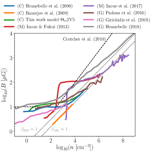
Figure 16: The mean field strength as a function of the gas density in various studies extracted from Hennebelle et al. (2008), Banerjee et al. (2009), Padoan et al. (2016), Hennebelle (2018), Inoue & Fukui (2013), Inoue et al. (2017), Girichidis et al. (2018). The $B$-$n$ relations are extracted by using WebPlotDigitizer (Rohatgi, 2021) except for Inoue & Fukui (2013) and Inoue et al. (2017). The two gray lines correspond to $\beta_{\mathrm{10K}}=1$ and $\beta_{\mathrm{20K}}=1$. The observational prediction in Crutcher et al. (2010), $B\sim\max(10~{}\mu\mathrm{G}(n/300~{}\mathrm{cm}^{-3})^{0.65},10~{}\mu\mathrm{G})$, is shown by the dashed line.

We also compare our $B$-$n$ relations with those of supernova-regulated ISM MHD simulations (Padoan et al., 2016; Hennebelle, 2018). Padoan et al. (2016) carry out a simulation with periodic boundary conditions in a simulation box of $(250~{}\mathrm{pc})^{3}$. Their results are consistent with our results although their simulation setup is quite different from ours. Hennebelle (2018) consider the stratification of the galactic disk, and their simulations resolve the gas dynamics from the kpc scale to $0.004~{}$pc by using a zoom-in technique. Their results show that the field strength follows $B\propto n^{1/2}$ for higher densities, but it is slightly stronger than that predicted from $\beta=1$ even when the gas density is as high as $10^{6}~{}\mathrm{cm}^{-3}$ if the gas temperature is as low as 10 K.

Mocz et al. (2017) performed isothermal simulations of driven turbulence with different initial field strengths, and demonstrated that the outer regions ($\sim 10^{4}~{}$au) of the cores have $\beta\sim 1$, regardless of the initial field strength. The regions of $B\propto n^{2/3}$, where gravitationally collapse isotropically, emerge on small scales ($r<10^{4}~{}$au) only when the initial Alfvén Mach number is less than unity. In our simulations, the phase of $B\propto n^{2/3}$ cannot be resolved because of the lack of resolution.

Li et al. (2015) found that the mean field strength of clumps does not follow $n^{1/2}$ but it is proportional to $n^{0.7}$, which is comparable to those found in observations of the Zeeman measurement (see Section 5.4.3). The mean field strength of their results is $B\sim 20~{}\mu\mathrm{G}\left(n/10^{4}~{}\mathrm{cm}^{-3}\right)^{0.7}$, regardless of the initial field strength. It is higher than those obtained in our simulations. An possible reason is the difference of the simulation setups. In our simulations, dense clumps evolve from the stable stage to the unstable stage through coalescence of smaller clumps and the gas accumulation of the atomic gas. By contrast, Li et al. (2015) prepared a gravitationally unstable gas as the initial condition. Rapid super-Alfvénic contraction of the dense clumps may lead to a strong density-dependence of the field strength ($B\propto n^{0.7}$).

In summary, the plasma $\beta$ in dense regions is order of unity in previous studies conducting colliding flow simulations (Hennebelle et al., 2008; Banerjee et al., 2009; Inoue & Fukui, 2013; Inoue et al., 2017). However, in other setups, some simulations show consistent results (Padoan et al., 2016; Girichidis et al., 2018), but some studies are not consistent with ours (Hennebelle, 2018; Li et al., 2015). Further investigations are needed to understand what makes this difference in the high density limit of the $B$-$n$ relation

5.4.3 $B$-$n$ Relations in Observational Studies

Analysing the results of Zeeman surveys of Hi, OH, and CN, Crutcher et al. (2010) derived an expected field strength as a function of density that is given by $B_{\mathrm{obs}}\sim 10~{}\mu\mathrm{G}(n/300~{}\mathrm{cm}^{-3})^{0.65}$ for $n>300~{}\mathrm{cm}^{-3}$. It is about three times stronger than our results at $n=10^{3}~{}\mathrm{cm}^{-3}$, and the difference increases with the density, indicating that the plasma $\beta$ of the observed clouds is much lower than unity. Crutcher (1999) found that the plasma $\beta$ is as low as $0.04^{+0.03}_{-0.02}$, which appears to be contradict with our results.

A reason of this discrepancy may come from the fact that the Zeeman surveys have mainly been conducted in massive star forming regions. Suppose that a spherical cloud with a density of $\rho$ and mass of $M$ has a magnetic field with a strength of $B$, the mass-to-flux ratio is given by

$$\frac{\mu}{\mu_{\mathrm{cri}}}=2\pi\sqrt{G}\frac{M}{B\pi(3M/4\pi\rho)^{2/3}}.$$ (55)

Solving equation (55) for $M$ using a relation of $B=c_{\mathrm{s}}\sqrt{8\pi\rho\beta^{-1}}$, one obtains

$$M = 10^{3}~{}\mathrm{M_{\odot}}~{}\left(\frac{\mu/\mu_{\mathrm{cri}}}{2}\right)^{3}\left(\frac{\beta}{0.04}\right)^{-3/2}$$ (56)

$$\left(\frac{c_{\mathrm{s}}}{0.2~{}\mathrm{km~{}s^{-1}}}\right)^{3}\left(\frac{n}{10^{4}~{}\mathrm{cm}^{-3}}\right)^{-1/2}.$$

The equation indicates that in order for a cloud with $\beta\sim 0.04$ to be gravitationally unstable, it should be massive. This is consistent with the fact that most data in high density range analyzed in Crutcher et al. (2010) are associated with massive star formation. Inoue & Fukui (2013) and Inoue et al. (2017) demonstrated that magnetically-supported dense cores formed by cloud-cloud collisions are possible sites of massive star formation (Figure 16). An averaged plasma $\beta$ of such dense cores is expected to be much lower than unity as seen in the Zeeman observations although the plasma beta of the central densest region is order of unity (Figure 16).

We focuses on low and intermediate mass star formation. For model $\Theta_{\mathrm{cr}}2$V10, a typical plasma $\beta$ and density of the post-shock gas are $\sim 0.025$ and $200~{}\mathrm{cm}^{-3}$, respectively, if we assume that the pre- and post-shock gas are uniform and isothermal with a sound speed of $0.3~{}\mathrm{km~{}s^{-1}}$. Only forty-times density enhancement is enough for the plasma $\beta$ to become unity. Thus, our results are not contradict with the observations measuring the field strength through the Zeeman effect.

5.5 Relative Orientations between Density Structures and Magnetic Fields

To characterize the relation between the density and magnetic fields, Soler et al. (2013) define that the angle $\varphi$ between the magnetic field and gradient of the density using the following expression:

$$\varphi=\tan^{-1}\left(\frac{|\mathbf{B}\times\mathbf{\nabla}n|}{\mathbf{B}\cdot\mathbf{\nabla}n}\right)$$ (57)

where $\mathbf{\nabla}n$ is calculated using the Gaussian derivative kernel with the standard deviation $\Delta x/\sqrt{2}$ to reduce numerical fluctuations.

The two-dimensional version of Equation (57), where $n$ is replaced by observed surface densities and the direction of $\mathbf{B}$ is estimated from polarization observations, is often used to link the simulation and observation studies (e.g., Planck Collaboration et al., 2016a).

Figure 17: Three-dimensional HROs obtained from the snapshots at $t=t_{\mathrm{first}}+0.5~{}$Myr for models (a) $\Theta_{\mathrm{cr}}0.25$V5, (b) $\Theta_{\mathrm{cr}}2$V5, (c) $\Theta_{\mathrm{cr}}0.25$V10, and (d) $\Theta_{\mathrm{cr}}2$V10. In each panel, the lines correspond to the HROs at the five different density bins.

Figure 17 shows the histogram of $\cos\varphi$ called Histogram of Relative Orientations (HROs), which was proposed by Soler et al. (2013). For the lowest density bin ($10^{2.5}~{}\mathrm{cm}^{-3}\leq n<10^{3}~{}\mathrm{cm}^{-3}$), the HROs have sharp peaks around $\cos\varphi\sim 0$ for all the models, indicating that the density structure tends to be elongated along the magnetic field. The directions of the density elongation are different between the models with $\theta=0.25\theta_{\mathrm{cr}}$ and $2\theta_{\mathrm{cr}}$. For $\theta=0.25\theta_{\mathrm{cr}}$, the strong shear motion, which is generated by the anisotropic super-Alfvénic turbulence (Figure 2c), stretches both the density structure and magnetic fields in the collision direction. By contrast, for $\theta=2\theta_{\mathrm{cr}}$, the magnetic fields amplified by the shock compression are perpendicular to the collision direction, and the gas is elongated along the magnetic field.

As the density increases, the peaks around $\cos\varphi\sim 0$ become less prominent while the number of counts around $\cos\varphi\sim\pm 1$ increases for all the models. The highest density bin ($10^{4.5}~{}\mathrm{cm}^{-3}\leq n\leq 10^{5}~{}\mathrm{cm}^{-3}$) corresponds to the densest clumps identified in this paper. Figure 17 shows that the HROs at the highest density bin depend on $\theta/\theta_{\mathrm{cr}}$. For $\theta=0.25\theta_{\mathrm{cr}}$, the HROs become almost flat, indicating that any angles between $\mathbf{\nabla}n$ and $\mathbf{B}$ are equally realized. For $\theta=2\theta_{\mathrm{cr}}$, the magnetic fields tend to be perpendicular to the direction of the elongation of the density structures for $n>10^{4}~{}\mathrm{cm}^{-3}$. This clearly reflects that the filamentary structures are elongated perpendicular to the magnetic field (the right panels of Figure 4).

These properties of the HROs are consistent with other simulation studies where the flip from the regime of $\mathbf{\nabla}n\perp\mathbf{B}$ to that of $\mathbf{\nabla}n\parallel\mathbf{B}$ occurs only in high magnetization cases with $\beta\ll 1$ (Soler et al., 2013; Barreto-Mota et al., 2021) although what determines the critical densities at which the flip occurs is not fully understood theoretically (Pattle et al., 2022). For the models with $\theta=2\theta_{\mathrm{cr}}$, the critical density ($\sim 10^{4}~{}\mathrm{cm}^{-3}$) roughly agrees with the mean density at which the dense clumps with $>1~{}M_{\odot}$ change from sub-critical to super-critical (Figure 12). This is consistent with the results of Seifried et al. (2020).

Planck Collaboration et al. (2016a, b) found that the relative angle $\varphi$ systematically changes with increasing surface density in a consistent way as the simulation results. With the clump mass $\sim 10~{}M_{\odot}$ around which $\alpha_{\mathrm{tot}}$ becomes less than unity (the bottom panels of Figure 11), the transition density $n\sim 10^{4}~{}\mathrm{cm}^{-3}$ corresponds to the surface density $N\sim n\times(4\pi/3\times(10~{}M_{\odot})/(1.4nm_{\mathrm{H}}~{}\mathrm{cm}^{-3}))^{1/3}\sim 10^{22}~{}\mathrm{cm}^{-2}$, which appears to be consistent with the value $N_{\mathrm{H}}\sim 10^{21.7}~{}\mathrm{cm}^{-2}$ obtained from the Planck observations (Planck Collaboration et al., 2016b). More rigorous comparisons will be made in forthcoming papers by applying synthetic observations to our results.

5.6 Density Dependence of Velocity Dispersions

Figures 9 and 10 show that the $\delta u_{\mathrm{cl,1D}}$-$R$ relations depends on the mean clump density although the dynamic range of the clump sizes is less than one decade. The density dependence is more significant for larger $V_{0}$. Observationally, the density-dependence of the $\delta u_{\mathrm{cl,1D}}$-$R$ relation can be investigated by using multiple lines of different molecules and isotopes (Goodman et al., 1998).

In the L1551 cloud in Taurus, which is an isolated low-mass star-forming region, Yoshida et al. (2010) do not find any clear deferences in the three line width-size relations ($\sigma_{\mathrm{NT}}\sim 0.2~{}\mathrm{km~{}s^{-1}}~{}(L/1~{}\mathrm{pc})^{0.5}$) obtained from the ¹²CO ($J=1-0)$, ¹³CO ($J=1-0$), and C¹⁸O ($J=1-0$) lines. The obtained velocity dispersions are transonic $\sim 0.2~{}\mathrm{km~{}s^{-1}}$ even at $L\sim 1~{}\mathrm{pc}$, and appear to be smaller than a typical line width-size relation (e.g., Larson, 1981; Solomon et al., 1987). This observational result may be qualitatively consistent with the models with $V_{0}=5~{}\mathrm{km~{}s^{-1}}$.

Recently, in the filamentary infrared dark cloud G034.43+00.24, Liu et al. (2022) found that the velocity dispersion-size relation in smaller scales ($\sim 0.09~{}$pc) gives systematically lower velocity dispersions than that in larger scales ($\sim 0.6~{}$pc). This may be qualitatively consistent with the models with $V_{0}=10~{}\mathrm{km~{}s^{-1}}$, which show the negative dependence of $\delta u_{\mathrm{cl,1D}}$ on the mean clump density (Figure 10).

On the other hand, Liu et al. (2022) found that the turbulence spectrum toward a filamentary infrared dark cloud G034.43+00.24 observed in the dense-gas tracer H¹³CO⁺ shows a systematic deviation from the Larson’s law and the slope is steeper. This may be qualitatively consistent with the models with $V_{0}=10~{}\mathrm{km~{}s^{-1}}$. We attribute this deviation from the Larson’s law to the gravitational collapse in the dense region.

5.7 Core Formation

We found that for $n>n_{\mathrm{grv}}$, $\mu/\mu_{\mathrm{cr}}$ becomes order of unity. This indicates that the magnetic energy is comparable to the gravitational energy. Since plasma beta is order of unity for $n>n_{\mathrm{grv}}$, the thermal energy is also comparable to the magnetic energy. In Section 5.2, we found that the Alfvén mach number is also order of unity for $n>n_{\mathrm{grv}}$. Combining these results suggests that all the energies (thermal, kinetic, magnetic, and gravitational energies) become equipartition when $n>n_{\mathrm{grv}}$, regardless of $\theta$. This property has been found in previous studies. Lee & Hennebelle (2019) for instance found that ${\cal E}_{\mathrm{mag}}$, ${\cal E}_{\mathrm{th}}$, and ${\cal E}_{\mathrm{grv}}$ reach equipartition in the high-density ends of their runs.

Chen & Ostriker (2014) found that core masses do not depend on the upstream magnetic field direction in their colliding-flow simulations. They estimated the core mass by using a theoretical argument considering gas accumulation along the magnetic field. In terms of our notation, their estimated core mass corresponds to the Jean mass with $n=n_{\mathrm{grv}}=\langle n_{0}\rangle\left(V_{0}/c_{\mathrm{s}}\right)^{2}\sim 10^{5}~{}\mathrm{cm}^{-3}$. From Equation (42), the cores with $n\sim n_{\mathrm{grv}}$ are expected to be super-critical when the core mass is around 1 $M_{\odot}$. Our results suggest that the contribution of the magnetic field to the virial theorem is negligible when $n>n_{\mathrm{grv}}/3=3\times 10^{4}~{}\mathrm{cm}^{-3}$ (Equation (38)). This is consistent with their results, which show that a typical core mass is independent of magnetic fields.

Chen & Ostriker (2015) investigated the dependence of the core properties on the collision speed and field strength. The plasma $\beta$ of the cores takes values roughly between 1 and 10, consistent with our results. They found that the core collapse time is proportional to $V_{0}^{-1/2}$ (also see Iwasaki & Tsuribe, 2008; Gong & Ostriker, 2011). This appears to be contradict with our results, which show that the clump formation time is insensitive to $V_{0}$ (Table 1 and Figure 3). This discrepancy may come from the difference in the disturbances of the pre-shock gas. Relatively weak turbulence ($\delta v=0.14~{}\mathrm{km~{}s^{-1}}$ in a box of $(1~{}\mathrm{pc})^{3}$) was considered in Chen & Ostriker (2015) while the two-phase structure of the atomic gas is considered in this paper. In our setting, higher collision speeds do not make the clump formation time shorter because stonger post-shock turbulence is driven.

5.8 Long-term Evolutions

In this paper, we focus on the early evolution of the dense clumps since our simulations are terminated at 0.5 Myr after the formation of the first unstable clump because a star formation treatment is not included and the resolution is not high enough to resolve very dense cores. In this section, we here discuss whether our results are applicable to the long-term evolution.

In the long-term evolutions, the clumps will grow through gas accretion and denser cores will form. The analytic formulae of the virial parameters shown in Equations (32), (34), and (36) are all applicable in the long-term evolutions. $\alpha_{\mathrm{th}}$ parameter (Equation (32)) is unlikely to change significantly unless the gas is heated up locally by the star formation. The magnetic energies of the dense clumps are strongly related with the $B$-$n$ relation. If the magnetic field amplification is caused by the gravitational contraction also in the long-term evolutions, Equation (36) is also unlikely to change significantly. It is possible that ${\cal E}_{\mathrm{kin}}$ increases as the gravitational potential becomes deeper (Arzoumanian et al., 2013), or $\delta u_{1}$ in Equation (34) increases. The long-term evolutions with higher resolution are investigated in forthcoming papers.

6 Summary

We investigated the formation and evolution of MCs by colliding flows of the atomic gas with a mean density of $\langle n_{0}\rangle=10~{}\mathrm{cm}^{-3}$ and field strength of $B_{0}=3~{}\mu$G. We additionally include self-gravity in the simulations done in Paper I and investigate the global properties of post-shock layers and the statistical properties of dense clumps.

As parameters, we consider the collision speed and the angle between the magnetic field and upstream flow. As examples of the turbulent-dominated and magnetic field-dominated layers, we adopt $\theta=0.25\theta_{\mathrm{cr}}$ and $2\theta_{\mathrm{cr}}$, respectively. The critical $\theta_{\mathrm{cr}}$ is found in Paper I and defined in Equation (7). We consider two collision speeds of $5~{}\mathrm{km~{}s^{-1}}$ and $10~{}\mathrm{km~{}s^{-1}}$.

Our findings are as follows:

1. The $\theta$-dependence of the physical properties of the post-shock layers affect on the clump formation.

   • For $\theta=0.25\theta_{\mathrm{cr}}$, anisotropic super-Alfvénic turbulence driven for $\theta=0.25\theta_{\mathrm{cr}}$ suppresses the formation of self-gravitating clumps. The post-shock layers are significanly disturbed by turbulence, and no prominent filamentary structures are found.

   • For $\theta=2\theta_{\mathrm{cr}}$, the gas accumulates along the shock amplified magnetic field, and prominent filamentary structures form.

   Self-gravitating clumps are formed more efficiently for $\theta=2\theta_{\mathrm{cr}}$ than for $\theta=0.25\theta_{\mathrm{cr}}$.

2. The difference of $V_{0}$ does not influence the epoch of the formation of the first unstable clump $t_{\mathrm{first}}$ significantly although the mass accumulation rate increases in proportion to $V_{0}$. This is because all the energies are in proportional to $V_{0}^{2}$, and their ratios are independent of $V_{0}$.

3. The parameter dependence of the field strength-density relation appears only for low densities. The mean field strength approaches a univeral relation that determined by $\beta\sim O(1)$ as the density increases, regardless of values of $\theta$ and $V_{0}$ (Figure 5). The critical density which divides the two asymptotic behaviors is expressed as $n_{\mathrm{grv}}=\langle n_{0}\rangle(V_{0}/c_{\mathrm{s}})^{2}$ (Equation (14)). We confirm that the $B$-$n$ relations derived in previous studies with different setups approach $\beta\sim O(1)$ in the high-density limit, consistent with our results (Figure 16).

4. The physical properties of the bulk velocities of dense clumps are inherited from the turbulence structure of the post-shock layers. The models with $\theta=0.25\theta_{\mathrm{cr}}$ show that the bulk velocities are biased in the collision direction for less dense clumps. As the clump density increases, the anisotropy of the bulk velocities becomes insignificant. Anisotropy in the bulk velocities is not found in the models with $\theta=2\theta_{\mathrm{cr}}$.

5. The internal velocity dispersions of dense clumps roughly obey $\propto R_{\mathrm{cl}}^{0.5}$, where $R_{\mathrm{cl}}$ is a typical clump radius, which is defined as $R_{\mathrm{cl}}=(3V_{\mathrm{cl}}/(4\pi))^{1/3}$, where $V_{\mathrm{cl}}$ is the volume of dense clumps. The internal velocity dispersions $\delta u_{\mathrm{cl,1D}}$ depend not on $\theta$ but on $V_{0}$. For diffuse clumps with $\sim 10^{3}~{}\mathrm{cm}^{-3}$, $\delta u_{\mathrm{cl,1D}}$ is roughly in proportion to $V_{0}$. The larger the collision speed, the faster $\delta u_{\mathrm{cl,1D}}$ decreases with the clump density. As a result, the parameter-dependence of $\delta u_{\mathrm{cl,1D}}$ becomes insignifiant for denser clumps.

6. The virial parameter $\alpha_{\mathrm{tot}}$ is divided into three contributions from the thermal pressure $\alpha_{\mathrm{th}}$, Raynolds stress $\alpha_{\mathrm{kin}}$, and Maxwell stress $\alpha_{\mathrm{mag}}$ in Equation (28). The thermal and magnetic virial parameters are proportional to $M_{\mathrm{cl}}^{-2/3}$ and kinetic virial parameter is proportional to $M_{\mathrm{cl}}^{-1/3}$, where $M_{\mathrm{cl}}$ is the clump mass. We develop an analytic formulae for $\alpha_{\mathrm{th}}$ in Equation (32), for $\alpha_{\mathrm{kin}}$ in Equation (34), and for $\alpha_{\mathrm{mag}}$ in Equation (36). They explain our results reasonably well.

7. We found that the mass-to-flux ratios of dense clumps with $\sim 1~{}M_{\odot}$ are expected to be order of unity if the clump density is higher than $n_{\mathrm{grv}}$ in a wide range of the collision parameters which reproduces the observed relations.

References

- Alves et al. (2008) Alves, F. O., Franco, G. A. P., & Girart, J. M. 2008, A&A, 486, L13
- André et al. (2010) André, P., Men’shchikov, A., Bontemps, S., et al. 2010, A&A, 518, L102
- Arzoumanian et al. (2013) Arzoumanian, D., André, P., Peretto, N., & Könyves, V. 2013, A&A, 553, A119
- Auddy et al. (2016) Auddy, S., Basu, S., & Kudoh, T. 2016, ApJ, 831, 46
- Audit & Hennebelle (2010) Audit, E., & Hennebelle, P. 2010, A&A, 511, A76
- Banerjee et al. (2009) Banerjee, R., Vázquez-Semadeni, E., Hennebelle, P., & Klessen, R. S. 2009, MNRAS, 398, 1082
- Barreto-Mota et al. (2021) Barreto-Mota, L., de Gouveia Dal Pino, E. M., Burkhart, B., et al. 2021, MNRAS, 503, 5425
- Bertoldi & McKee (1992) Bertoldi, F., & McKee, C. F. 1992, ApJ, 395, 140
- Blitz et al. (2007) Blitz, L., Fukui, Y., Kawamura, A., et al. 2007, Protostars and Planets V, 81
- Chapman et al. (2011) Chapman, N. L., Goldsmith, P. F., Pineda, J. L., et al. 2011, ApJ, 741, 21
- Chen & Ostriker (2014) Chen, C.-Y., & Ostriker, E. C. 2014, ApJ, 785, 69
- Chen & Ostriker (2015) —. 2015, ApJ, 810, 126
- Crutcher (1999) Crutcher, R. M. 1999, ApJ, 520, 706
- Crutcher et al. (2010) Crutcher, R. M., Wandelt, B., Heiles, C., Falgarone, E., & Troland, T. H. 2010, ApJ, 725, 466
- Dib et al. (2007) Dib, S., Kim, J., Vázquez-Semadeni, E., Burkert, A., & Shadmehri, M. 2007, ApJ, 661, 262
- Dobbs & Wurster (2021) Dobbs, C. L., & Wurster, J. 2021, MNRAS, 502, 2285
- Elsässer & Schamel (1976) Elsässer, K., & Schamel, H. 1976, Z. Physik B., 23, 89
- Field (1965) Field, G. B. 1965, ApJ, 142, 531
- Field et al. (1969) Field, G. B., Goldsmith, D. W., & Habing, H. J. 1969, ApJ, 155, L149
- Fukui et al. (2017) Fukui, Y., Tsuge, K., Sano, H., et al. 2017, PASJ, 69, L5
- Fukui et al. (2009) Fukui, Y., Kawamura, A., Wong, T., et al. 2009, ApJ, 705, 144
- Girichidis et al. (2018) Girichidis, P., Seifried, D., Naab, T., et al. 2018, MNRAS, 480, 3511
- Gong & Ostriker (2011) Gong, H., & Ostriker, E. C. 2011, ApJ, 729, 120
- Gong et al. (2017) Gong, M., Ostriker, E. C., & Wolfire, M. G. 2017, ApJ, 843, 38
- Goodman et al. (1998) Goodman, A. A., Barranco, J. A., Wilner, D. J., & Heyer, M. H. 1998, ApJ, 504, 223
- Heiles & Troland (2005) Heiles, C., & Troland, T. H. 2005, ApJ, 624, 773
- Heitsch et al. (2009) Heitsch, F., Stone, J. M., & Hartmann, L. W. 2009, ApJ, 695, 248
- Hennebelle (2018) Hennebelle, P. 2018, A&A, 611, A24
- Hennebelle et al. (2008) Hennebelle, P., Banerjee, R., Vázquez-Semadeni, E., Klessen, R. S., & Audit, E. 2008, A&A, 486, L43
- Hennebelle & Pérault (2000) Hennebelle, P., & Pérault, M. 2000, A&A, 359, 1124
- Hunter (2007) Hunter, J. D. 2007, Computing in Science and Engineering, 9, 90
- Iffrig & Hennebelle (2017) Iffrig, O., & Hennebelle, P. 2017, A&A, 604, A70
- Indriolo et al. (2007) Indriolo, N., Geballe, T. R., Oka, T., & McCall, B. J. 2007, ApJ, 671, 1736
- Indriolo et al. (2015) Indriolo, N., Neufeld, D. A., Gerin, M., et al. 2015, ApJ, 800, 40
- Inoue & Fukui (2013) Inoue, T., & Fukui, Y. 2013, ApJ, 774, L31
- Inoue et al. (2017) Inoue, T., Hennebelle, P., Fukui, Y., et al. 2017, PASJ in press
- Inoue & Inutsuka (2009) Inoue, T., & Inutsuka, S. 2009, ApJ, 704, 161
- Inoue & Inutsuka (2012) —. 2012, ApJ, 759, 35
- Iwasaki et al. (2019) Iwasaki, K., Tomida, K., Inoue, T., & Inutsuka, S. 2019, ApJ, 873, 6
- Iwasaki & Tsuribe (2008) Iwasaki, K., & Tsuribe, T. 2008, PASJ, 60, 125
- Kobayashi et al. (2020) Kobayashi, M. I. N., Inoue, T., Inutsuka, S., et al. 2020, ApJ, 905, 95
- Kobayashi et al. (2022) Kobayashi, M. I. N., Inoue, T., Tomida, K., Iwasaki, K., & Nakatsugawa, H. 2022, ApJ, 930, 76
- Körtgen & Banerjee (2015) Körtgen, B., & Banerjee, R. 2015, MNRAS, 451, 3340
- Koyama & Inutsuka (2000) Koyama, H., & Inutsuka, S. 2000, ApJ, 532, 980
- Koyama & Inutsuka (2002) —. 2002, ApJ, 564, L97
- Lada et al. (2008) Lada, C. J., Muench, A. A., Rathborne, J., Alves, J. F., & Lombardi, M. 2008, ApJ, 672, 410
- Landau & Lifshitz (1959) Landau, L. D., & Lifshitz, E. M. 1959, Fluid mechanics
- Larson (1981) Larson, R. B. 1981, MNRAS, 194, 809
- Lee & Hennebelle (2019) Lee, Y.-N., & Hennebelle, P. 2019, A&A, 622, A125
- Li et al. (2015) Li, P. S., McKee, C. F., & Klein, R. I. 2015, MNRAS, 452, 2500
- Liu et al. (2022) Liu, H.-L., Tej, A., Liu, T., et al. 2022, MNRAS, 511, 4480
- McCray & Kafatos (1987) McCray, R., & Kafatos, M. 1987, ApJ, 317, 190
- McKee & Ostriker (1977) McKee, C. F., & Ostriker, J. P. 1977, ApJ, 218, 148
- McKee & Zweibel (1992) McKee, C. F., & Zweibel, E. G. 1992, ApJ, 399, 551
- Mestel (1965) Mestel, L. 1965, QJRAS, 6, 265
- Mocz et al. (2017) Mocz, P., Burkhart, B., Hernquist, L., McKee, C. F., & Springel, V. 2017, ApJ, 838, 40
- Mouschovias (1976) Mouschovias, T. C. 1976, ApJ, 207, 141
- Mouschovias & Spitzer (1976) Mouschovias, T. C., & Spitzer, Jr., L. 1976, ApJ, 210, 326
- Myers & Goodman (1988) Myers, P. C., & Goodman, A. A. 1988, ApJ, 329, 392
- Nakano & Nakamura (1978) Nakano, T., & Nakamura, T. 1978, PASJ, 30, 671
- Nelson & Langer (1999) Nelson, R. P., & Langer, W. D. 1999, ApJ, 524, 923
- Neufeld & Wolfire (2017) Neufeld, D. A., & Wolfire, M. G. 2017, ApJ, 845, 163
- Padoan et al. (2016) Padoan, P., Pan, L., Haugbølle, T., & Nordlund, Å. 2016, ApJ, 822, 11
- Parker (1953) Parker, E. N. 1953, ApJ, 117, 431
- Pattle et al. (2022) Pattle, K., Fissel, L., Tahani, M., Liu, T., & Ntormousi, E. 2022, arXiv e-prints, arXiv:2203.11179