Space-time unfitted finite element methods for time-dependent problems on moving domains

Abstract.

We propose a space-time scheme that combines an unfitted finite element method in space with a discontinuous Galerkin time discretisation for the accurate numerical approximation of parabolic problems with moving domains or interfaces. We make use of an aggregated finite element space to attain robustness with respect to the cut locations. The aggregation is performed slab-wise to have a tensor product structure of the space-time discrete space, which is required in the numerical analysis. As an aternative, we also propose a space-time ghost penalty stabilisation term to attain robustness. We analyse the proposed algorithm, providing stability, condition number bounds and anisotropic a priori error estimates. A set of numerical experiments confirm the theoretical results for a parabolic problem on a moving domain. The method is applied for a mass transfer problem with changing topology.

Keywords: Embedded methods; unfitted finite elements; space-time discretisations.

1. Introduction

Numerical simulations using standard finite element methods require the generation of body-fitted meshes, which is one of the main bottlenecks of the simulation workflow. This problem is exacerbated in applications that involve moving interfaces and evolving geometries. The method of lines, which discretises in space and time separately, cannot be readily applied to transient problems with moving domains or interfaces since it assumes a constant geometry in time. In order to solve this problem, one can consider arbitrary Lagrangian Eulerian (ALE) schemes [22, 43]. ALE schemes require frequent remeshing and are not suitable for large geometrical variations or topological changes. Another approach is to use variational space-time formulations on space-time body-fitted meshes. These methods have been widely used in applications like fluid-structure interaction [53, 10, 51]. Even though variational space-time schemes can be applied to moving domains/interfaces, they do require space-time meshes, which are unfeasible in general. The mathematical analysis of space-time methods has been considered, e.g., in [46] (for a discontinuous Galerkin (DG) method in time for parabolic equations on body-fitted domains and constant geometries) and in [50] (for a space-time DG method for advection-diffusion on time-dependent domains).

Unfitted (also known as immersed or embedded) finite element (FE) formulations lower the geometrical requirements since they do not require body-fitted meshes but simple, e.g., Cartesian, background meshes. Hence, unfitted FEM are becoming increasingly popular in applications with moving interfaces such as fluid-structure interactions [25, 14, 48], fracture mechanics [26, 21], and in applications with changing geometries such as additive manufacturing [41, 18] and stochastic geometry problems [4]. In [32], a mass transport problem across an evolving interface is analysed using a variational space-time DG extended finite element method (XFEM).

However, unfitted FEMs are prone to ill-conditioning problems when dealing with unfitted boundaries and high contrast interface problems [45, 3, 15]. If the intersection of a cut background cell with the physical domain is small, it can lead to a so-called small cut cell problem. The support of the FE shape functions corresponding to the background cell can have an arbitrarily small support, leading to almost singular system matrices. Several methods [15, 31, 33, 28, 36] have been proposed to circumvent the small cut cell problem. However, only few formulations are robust and optimal with respect to the cut cell position. Some methods include additional terms that enhance the stability of the FE discretisation while keeping optimal convergence (see, e.g., the ghost penalty [13] formulation used in CutFEM [15, 57, 20]). Another approach, used in this work, involves cell aggregation (or agglomeration) techniques. These techniques can readily be applied to numerical methods that can handle general polytopal meshes, e.g., DG or hybridisable methods (see, e.g., [9, 47, 23, 17]). Cell aggregation for $\mathcal{C}^{0}$ FE spaces has been proposed in [3], where it was coined aggregated finite element method (AgFEM).

In AgFEM, the degrees of freedom associated to FE functions that have arbitrarily small support and can lead to ill-conditioning are eliminated. This is attained by designing a discrete extension operator that constrains the ill-posed DOFs using the well-posed DOFs while preserving $\mathcal{C}^{0}$ continuity. AgFEM enjoys good numerical properties, such as stability, bounded condition numbers, optimal convergence and continuity with respect to data; detailed mathematical analysis of this method is included in [3] for elliptic problems, in [2] for the Stokes equation and in [8] for higher-order FEs. The method is also amenable to arbitrarily complex 3D geometries [6], distributed implementations for large scale problems [55], error-driven $h$-adaptivity and parallel tree-based meshes [5], explicit time-stepping for the wave equation [16] and elliptic interface problems with high contrast [40]. A weak AgFEM technique is proposed in [7], which is much less sensitive to stabilisation parameters than the ghost penalty method.

Despite the potential of unfitted FEMs for transient problems with moving boundaries and interfaces, few formulations are robust and enjoy optimal convergence. The space-time DG XFEM scheme proposed in [32] is not robust to the cut location and the error estimate is suboptimal with respect to time. The main reason for the suboptimal error estimates is the fact that the FE space cannot be expressed as a slab-wise tensor product in space-time. The CutFEM formulation in [57] makes use of space-time quadratures to approximate moving domains for transient convection-diffusion problems. Robust and optimally convergent space-time DG formulations are presented in [30, 29, 44], in which the robustness of these methods are due to additional stabilisation terms in the weak formulation. Space-time CutFEM on overlapping meshes with optimal convergence are explored in [37, 38].

The novelties of this work are the following:

1. We propose a novel unfitted variational space-time formulation on moving domains/interfaces that is robust with respect to the small cut cell problem. Robustness is attained by extending AgFEM to space-time. The spatial discretisation can handle both continuous (nodal) and discontinuous FE spaces, while a DG space is used in time.

2. We carry out a detailed mathematical analysis proving that this method enjoys sought-after numerical properties such as well-posedness, stability, bounded condition numbers and optimal convergence. In addition, we provide implementation details and perform a set of numerical experiments that support the theoretical results.

In particular, we consider a slab-wise cell aggregation scheme and a space-time discrete extension operator that can be expressed as a space-time tensor product. This way, the aggregated finite element (AgFE) space is constant at each time slab, and we can prove optimal error bounds.

The outline of this work is as follows. First, we introduce the embedded geometry setup, the aggregation strategy and construct the AgFE spaces in Section 2. In Section 3, the proposed space-time AgFEM discretisation is introduced for a model problem. We perform the numerical analysis of the method in Section 4 and numerical experiments that support these results are presented in Section 5. Finally, we draw some conclusions in Section 6.

2. Space-time aggregated finite element method

2.1. Embedded geometry setup

In this section, we provide a set of geometrical definitions that will be required to define the proposed formulation. We refer to Figure 1 for an illustration of many of the definitions below.

Let us consider an open, bounded, connected Lipschitz domain $\Omega^{0}\subset\mathbb{R}^{d}$, with $d\in\{2,3\}$ the number of spatial dimensions, a time domain $[0,T]$ and a smooth diffeomorphism $\boldsymbol{\varphi}_{t}(\boldsymbol{x}):\Omega^{0}\rightarrow\mathbb{R}^{d}$ for any $t\in[0,T]$. We define $\Omega(t)\doteq\left\{\boldsymbol{\varphi}_{t}(\boldsymbol{x})\ :\ \boldsymbol{x}\in\Omega^{0}\right\}$ (the domain at a given time step) and $Q=\left\{\boldsymbol{x}\in\Omega(t)\ :\ t\in[0,T]\right\}$ (the space-time domain). For simplicity, we assume that $Q$ is a polytopal domain. $\partial\Omega(t)$ represents the boundary of $\Omega(t)$. We consider a partition of the boundary into $\partial\Omega_{D}(t)$ and $\partial\Omega_{N}(t)$, the Dirichlet and Neumann spatial boundaries, resp. Thus, $\partial\Omega(t)=\partial\Omega_{D}(t)\cup\partial\Omega_{N}(t)$ and $\partial\Omega_{D}(t)\cap\partial\Omega_{N}(t)=\emptyset$. The Dirichlet and Neumann boundaries of the space-time domain are $\partial Q_{D}\doteq\cup_{t\in(0,T)}\partial\Omega_{D}(t)\times\{t\}$ and $\partial Q_{N}\doteq\cup_{t\in(0,T)}\partial\Omega_{N}(t)\times\{t\}$, resp. The boundary of $Q$ is $\partial Q\doteq\Omega(0)\cup\Omega(T)\cup\partial Q_{D}\cup\partial Q_{N}$.

Let us define a spatial artificial domain $\Omega_{art}\subset\mathbb{R}^{d}$ such that $\Omega(t)\subset\Omega_{art}$ for all $t\in[0,T]$. One can consider a simple geometry for $\Omega_{art}$, e.g., a bounding box, which can be meshed using a Cartesian grid. We can also define the space-time artificial domain $Q_{art}\doteq\Omega_{art}\times[0,T]$, such that $Q\subset Q_{art}$.

Let $0=t^{0}<t^{1}<\dots<t^{N}=T$ and $J^{n}\doteq(t^{n-1},t^{n}),1\leq n\leq N$, denote the $n$-th time slab. $\left\{J^{n}\right\}_{n=1}^{N}$ is a partition of $[0,T]$. The size of each time slab $J^{n}$ is denoted by $\tau^{n}\doteq t^{n}-t^{n-1}$ (the so-called time step size) and $\tau\doteq\max_{n=1,\ldots,N}\tau^{n}$. The artificial domain and the space-time domain corresponding to a time slab $J^{n}$ are denoted as $Q^{n}_{art}\doteq\Omega_{art}\times J^{n}$ and $Q^{n}\doteq\cup_{t\in J^{n}}\Omega(t)\times\{t\}$, resp. Furthermore, the intersection of the Dirichlet and Neumann boundaries with $Q^{n}_{art}$ are denoted as $\partial Q^{n}_{D}$ and $\partial Q^{n}_{N}$, resp. We also use the notation $\Omega^{n}\doteq\Omega(t^{n})$, $n=0,\ldots,N$.

Let $\bar{\mathcal{T}}_{h,art}^{n}$ be a conforming, shape regular and quasi-uniform partition of $\Omega_{art}$. The space-time mesh $\mathcal{T}_{h,art}^{n}$ is the Cartesian product of $\bar{\mathcal{T}}_{h,art}^{n}$ and $J^{n}$, i.e.,

$$\mathcal{T}_{h,art}^{n}\doteq\{\bar{T}\times J^{n}\in\mathcal{T}_{h,art}\ :\ \bar{T}\in\bar{\mathcal{T}}_{h,art}^{n}\}.$$

The super-index $n$ in $\bar{\mathcal{T}}_{h,art}^{n}$ stands for the fact that the background mesh can be different at different time slabs. E.g., $\bar{\mathcal{T}}_{h,art}^{n}$ can be a background $n$-tree mesh with adaptive mesh refinement. We use the notation $T^{n}$ for cells in $\mathcal{T}_{h,art}^{n}$ and $\bar{T}^{n}$ for cells in $\bar{\mathcal{T}}_{h,art}^{n}$. By construction, we can define the injective map $\bar{\cdot}:\mathcal{T}_{h,art}^{n}\longrightarrow\bar{\mathcal{T}}_{h,art}^{n}$ such that $T^{n}=\bar{T}^{n}\times J^{n}$, i.e., a map from space-time to space-only cells at each time slab. In the analysis, we assume that $\bar{\mathcal{T}}_{h,art}^{n}$ is a shape-regular and quasi-uniform mesh with characteristic cell size $h$.

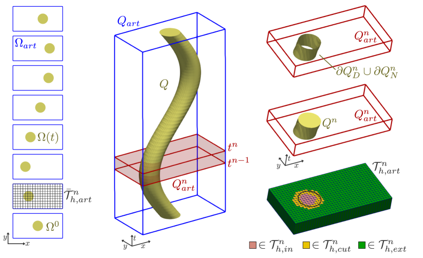
Figure 1. Graphical representation of the main geometrical quantities associated with the space-time embedded finite element setup for a 2D+1D example. We note in the figure at the bottom-right corner that some cells that are not cut on $t^{n}$ appear as cut. This is because these cells are cut at some time value $t\in[t^{n-1},t^{n}]$.

2.2. Cell aggregation

The direct use of unfitted FEMs on the previously defined meshes is not robust with respect to cut locations. As commented in the introduction, one could consider using stabilisation techniques to remedy this problem. Another approach, which is followed in this work, relies on the definition of aggregated or agglomerated meshes. In particular, cells are aggregated in such a way that all aggregates have a large enough portion inside the physical domain, e.g., there is one internal cell per aggregate.

We refer to [3] for the aggregation strategy required in the space-only case. In space-time, we apply this algorithm slab-wise to prevent cells at different time slabs to be merged to form aggregates. That would complicate the implementation and numerical analysis and have a serious impact on the computational cost. Our motivation is to end up with a space-time solver that only requires a set of sequential slab-wise solvers, as time marching methods.

The aggregation algorithm requires a classification of active cells between well-posed and ill-posed cells. The most straightforward definition is to classify interior cells as well-posed and cut cells as ill-posed. If ${T}^{n}\subset Q^{n}$, then ${T}^{n}$ is an internal cell. If ${T}^{n}\cap Q^{n}=\emptyset$, then ${T}^{n}$ is an external cell. Otherwise, ${T}^{n}$ is a cut cell. The set of internal, external and cut cells on time slab $J^{n}$ are denoted as $\mathcal{T}_{h,in}^{n}$, $\mathcal{T}_{h,ext}^{n}$ and $\mathcal{T}_{h,cut}^{n}$, resp. (see Figure 1). The union of internal, external and cut cells on each time slab is denoted as $Q_{in}^{n}\subset Q$, $Q_{ext}^{n}$ and $Q_{cut}^{n}$, resp. We define the set of active cells as $\mathcal{T}^{n}_{h,act}\doteq\mathcal{T}^{n}_{h,in}\cup\mathcal{T}^{n}_{h,cut}$ and their union as $Q^{n}_{act}$. We can readily define the space-only meshes $\bar{\mathcal{T}}^{n}_{h,act}\doteq\bar{\mathcal{T}}^{n}_{h,in}\cup\bar{\mathcal{T}}^{n}_{h,cut}$ using the map $\bar{\cdot}$ over the cells of the respective space-time meshes. The union of cells in $\bar{\mathcal{T}}_{h,act}^{n}$ is represented with $\Omega_{act}^{n}$.

This definition can be further refined by considering a numerical parameter $\eta_{0}>0$. Given a time slab $J^{n}$, one can compute the cell-wise quantity

$$\eta^{n}(T^{n})=\underset{t\in J^{n}}{\mathrm{min}}\frac{|\bar{T}^{n}\cap\Omega(t)|}{|\bar{T}^{n}|},\qquad\forall T^{n}\in\mathcal{T}_{h,act}^{n}.$$

If $\eta^{n}(T^{n})\geq\eta_{0}$, then $T^{n}$ is a well-posed cell. Otherwise, it is ill-posed. Note that this definition enforces that any space-time cell must have a significant portion in the spatial domain at all times, thus it is anisotropic. When $\eta_{0}=1$, then well-posed cells are internal cells and ill-posed cells are cut cells. For brevity, we will consider this case in the following exposition, even though the general case does not involve any modification.

Next, at each time slab, the aggregation strategy introduced in [3] (in a spatial mesh only) is performed on the active mesh $\mathcal{T}_{h,act}^{n}$. Very briefly, the algorithm performs the following steps: (1) well-posed cells are marked as touched first; (2) each ill-posed cell that is neighbour of touched cells is merged to one of these and marked as touched; (3) repeat (2) till all active cells are touched. This algorithm returns a set of aggregates $\mathrm{ag}(\mathcal{T}_{h,act}^{n})$ that contain one and only one well-posed cell. This well-posed cell is called the root cell of the aggregate. We refer to [3] for more details about the aggregation strategy in space, e.g., bounds for the size of the resulting aggregates.

2.3. Space-time unfitted FE spaces

Our aim is to construct AgFE spaces on each time slab making use of the aggregated meshes defined above. We start by introducing some notations. It is crucial to note that the AgFE spaces on each time slab may be different, even if $\mathcal{T}_{h,art}^{n}$ is the same for all slabs, due to the evolving geometry in time.

Let $T^{n}=\bar{T}^{n}\times J^{n}\in\mathcal{T}_{h,act}^{n}$, where $\bar{T}^{n}\in\bar{\mathcal{T}}_{h,act}^{n}$. We define the local FE space as a tensor product of spatial and temporal polynomials. For $d-$simplex spatial meshes, the local FE space ${V}({{T}^{n}})\doteq\mathcal{P}_{p}({\bar{T}^{n}})\otimes\mathcal{P}_{q}({J^{n}})$ is the space of polynomials of order less than or equal to $p$ in the spatial variables $x_{1},x_{2},\dots,x_{d}$ and polynomials of order less than or equal to $q$ in the temporal variable. For $d-$cube spatial meshes the local FE space ${V}({{T}^{n}})\doteq\mathcal{Q}_{p}({\bar{T}^{n}})\otimes\mathcal{P}_{q}({J^{n}})$ is the space of polynomials of order less than or equal to $p$ in each of the spatial variables $x_{1},x_{2},\dots,x_{d}$ and polynomials of order less than or equal to $q$ in the temporal variable.

In this work, we restrict ourselves to Lagrangian FE methods. Observe that the basis of the local FE space $V({{T}^{n}})$ is the tensor product of the Lagrangian basis of order $p$ in space and a basis for univariate polynomials of order $q$ in time. (The choice of a basis in time is flexible, since we will not enforce $\mathcal{C}^{0}$ continuity in time, but we will consider a Lagrangian basis for simplicity.) Let $\mathcal{N}({{T}^{n}})$ denote the set of Lagrangian nodes of ${{T}^{n}}$; any $a\in\mathcal{N}({{T}^{n}})$ can be expressed as a tuple $(a_{\boldsymbol{x}},a_{t})$ of space and time nodes. The dual basis of DOFs corresponds to the pointwise evaluation at these nodes. Analogously, the space-time shape functions associated to node $b\in\mathcal{N}({{T}^{n}})$ can be expressed as $\Phi^{b}(\boldsymbol{x},t)\doteq\phi^{b_{\boldsymbol{x}}}(\boldsymbol{x})\varphi^{b_{t}}(t)$, i.e., the tensor product of a spatial shape function $\phi^{b_{\boldsymbol{x}}}(\boldsymbol{x})$ and temporal shape function $\varphi^{b_{t}}(t)$. It satisfies $\Phi^{b}({\boldsymbol{x}}^{a_{\boldsymbol{x}}},t^{a_{t}})=\phi^{b_{\boldsymbol{x}}}({\boldsymbol{x}}^{a_{\boldsymbol{x}}})\varphi^{b_{t}}(t^{a_{t}})=\delta_{a_{\boldsymbol{x}}b_{\boldsymbol{x}}}\delta_{a_{t}b_{t}}$, where ${\boldsymbol{x}}^{a_{\boldsymbol{x}}}$ and $t^{a_{t}}$ are the spatial and temporal coordinates of the node $a$, resp., and $\delta$ is the Kronecker delta.

We consider a continuous Galerkin (CG) global FE space in the spatial direction at each time slab $J^{n}$. For CG methods, this is attained (on conforming meshes) by a local-to-global DOF map such that the resulting global space of functions is $\mathcal{C}^{0}$ continuous. To this end, at time slab $J^{n}$, we introduce the active space-time FE space

$$V_{h,act}^{n}\doteq\{v\in\mathcal{C}^{0}(Q^{n}_{act}):v|_{T}\in V(T),\text{ for any }T\in\mathcal{T}_{h,act}^{n}\}.$$

It can also be defined as a tensor-product space as follows. We define a space-only global FE space on $\Omega_{act}^{n}$ as

$$\bar{V}_{h,act}^{n}=\{v\in\mathcal{C}^{0}(\Omega_{act}^{n}):v|_{\bar{T}}\in\mathcal{X}_{p}(\bar{T}),\text{ for any }\bar{T}\in\bar{\mathcal{T}}_{h,act}^{n}\},$$

where $\mathcal{X}_{p}(\bar{T})$ is $\mathcal{P}_{p}(\bar{T})$ for simplicial meshes and $\mathcal{Q}_{p}(\bar{T})$ for hexahedral meshes. With all these ingredients, $V_{h,act}^{n}$ can be equivalently defined as $V_{h,act}^{n}\doteq\bar{V}_{h,act}^{n}\otimes\mathcal{P}_{q}(J^{n})$. We can proceed analogously for interior cells to define $V_{h,in}^{n}\doteq\bar{V}_{h,in}^{n}\otimes\mathcal{P}_{q}(J^{n})$.

Since we consider a DG approximation in time, the global space-time space can readily be defined as a Cartesian product of the above defined slab-wise spaces. In any case, the global problem is never solved at once but sequentially slab-by-slab.

2.4. Space-time AgFE spaces

It has been established that solving the FE problem on the active space leads to ill-conditioning problems. Therefore, we use an AgFE space to solve this issue. The key idea of AgFEM is to eliminate the problematic DOFs using well-posed DOFs. This is achieved by defining a discrete extension operator. Let $\bar{\mathcal{E}}:\bar{V}_{h,in}\rightarrow\bar{V}_{h,act}$ be the spatial extension operator between space-only interior $\bar{V}_{h,in}$ and active $\bar{V}_{h,act}$ FE spaces. The space-only discrete extension operator has been previously described, e.g., in [3]. The spatial AgFE space is defined as $\bar{V}_{h,ag}\doteq\bar{\mathcal{E}}(\bar{V}_{h,in})$. The discrete extension operator relies on a set of linear constraints that constrain the ill-posed DOFs (i.e., the ones that only belong to ill-posed cells) by the well-posed DOFs (the ones that belong to at least one well-posed cell). We do not provide the full construction of the space-only operator for the sake of conciseness. The interested reader can find the complete definition in [3] for the case of conforming background meshes, [5] for non-conforming adaptive meshes and [8] for a version of this extension that is well-suited to high-order approximations. The space-time extension proposed herein can be applied in all these situations.

In this work, we must define a slab-wise space-time discrete extension operator between $V_{h,in}^{n}$ and $V_{h,act}^{n}$. We do this by combining the slab-wise aggregation algorithm in Section 2.2, the tensor-product definition of these spaces in Section 2.3 and the space-only extension operator in [3]. In particular, at time slab $J^{n}$, the space-time extension operator $\mathcal{E}^{n}:V_{h,in}^{n}\rightarrow V_{h,act}^{n}$ is defined as follows:

$$\mathcal{E}^{n}(V_{h,in}^{n})=\mathcal{E}^{n}(\bar{V}_{h,in}^{n}\otimes\mathcal{P}_{q}(J^{n}))=\bar{\mathcal{E}}^{n}(\bar{V}_{h,in}^{n})\otimes\mathcal{P}_{q}(J^{n}),$$ (1)

where $\bar{\mathcal{E}}^{n}:\bar{V}_{h,in}^{n}\rightarrow\bar{V}_{h,act}^{n}$ is a space-only extension operator at slab $J^{n}$. The space-time aggregated FE space on the time slab, $V^{n}_{h,ag}\doteq\mathcal{E}^{n}(V_{h,in}^{n})$. The global space-time AgFE space is $\mathcal{V}_{h,ag}\doteq V^{1}_{h,ag}\times\dots\times V^{N}_{h,ag}$. By construction, we have $\mathcal{E}^{n}(u_{h})(\boldsymbol{x},t)=\bar{\mathcal{E}}^{n}(u_{h}(\cdot,t))(\boldsymbol{x})$ for $u_{h}\in V_{h,in}^{n}$.

3. Approximation of parabolic problems on moving domains

3.1. Model problem

We start by introducing some anisotropic functional spaces. Let $\boldsymbol{\alpha}=(\alpha_{1},\alpha_{2},\dots,\alpha_{d})$ and $|\boldsymbol{\alpha}|=\alpha_{1}+\dots+\alpha_{d}$. We define the anisotropic Sobolev space of order $(s_{s},s_{t})$ on a domain $\mathcal{D}\subset\mathbb{R}^{d+1}$ as

$$H^{(s_{s},s_{t})}(\mathcal{D})\doteq\{u\in L^{2}(\mathcal{D}):\partial^{\alpha_{1}}_{x_{1}}\dots\partial^{\alpha_{d}}_{x_{d}}u,\,\partial^{\beta}_{t}u\in L^{2}(\mathcal{D})\text{ for }|\boldsymbol{\alpha}|\leq s_{s},\beta\leq s_{t}\}.$$ (2)

The norm and semi-norm associated with this Sobolev space are:

$$\|v\|_{H^{(s_{s},s_{t})}(\mathcal{D})}^{2} \doteq\sum\limits_{\begin{subarray}{c}|\boldsymbol{\alpha}|\leq s_{s}\end{subarray}}\left\|\partial^{\alpha_{1}}_{x_{1}}\dots\partial^{\alpha_{d}}_{x_{d}}v\right\|^{2}_{L^{2}(\mathcal{D})}+\sum\limits_{\begin{subarray}{c}\beta\leq s_{t}\end{subarray}}\left\|\partial^{\beta}_{t}v\right\|^{2}_{L^{2}(\mathcal{D})},$$ (3)

$$|v|_{H^{(s_{s},s_{t})}(\mathcal{D})}^{2} \doteq\sum\limits_{\begin{subarray}{c}|\boldsymbol{\alpha}|=s_{s}\end{subarray}}\left\|\partial^{\alpha_{1}}_{x_{1}}\dots\partial^{\alpha_{d}}_{x_{d}}v\right\|^{2}_{L^{2}(\mathcal{D})}+\left\|\partial^{s_{t}}v\right\|^{2}_{L^{2}(\mathcal{D})}.$$

We introduce the proposed formulation for the convection-diffusion equation on moving domains with non-homogeneous boundary conditions as a model problem. In any case, the proposed methodology can be extended to other parabolic problems. Using the ideas in [2], it can also be generalised to indefinite systems, e.g., incompressible flows.

We represent with $H_{g_{D}}^{(1,s_{t})}(Q)$ the subspace of function in $H^{(1,s_{t})}(Q)$ with trace $g_{D}\in H^{(1/2,s_{t})}(\partial Q_{D})$ on the Dirichlet boundary. The model problem seeks to find $u:Q\rightarrow\mathbb{R}\in H^{(1,0)}_{g_{D}}(Q)\cap H^{(-1,1)}(Q)$ such that

$$\partial_{t}u+\boldsymbol{w}\cdot\boldsymbol{\nabla}u-\mu\Delta u=f H^{(-1,0)}(Q),\qquad \mu\nabla u\cdot\boldsymbol{n}=g_{N} H^{(-1/2,0)}(\partial Q_{N}),$$ in in (4)

and the initial condition $u(x,0)=u^{0}(x)\in L^{2}(\Omega^{0})$, where $\mu$ is the diffusion coefficient, the source term $f\in H^{(-1,0)}(Q)$, $\boldsymbol{w}\in L^{\infty}(Q)$ is a solenoidal convective field, the boundary flux $g_{N}\in H^{(-1/2,0)}(\partial Q_{N})$ and $\boldsymbol{n}$ denotes the outward normal to the boundary $\partial Q_{N}$. The weak form of (4) consists in finding

$$u\in H_{g_{D}}^{(1,0)}(Q)\cap H^{(-1,1)}(Q)\quad:\quad B(u,v)=L(v)\qquad\forall v\in H^{(1,0)}(Q),$$ (5)

where

$$B(u,v) =\int_{Q}\partial_{t}u\mathrm{~{}}v\mathrm{~{}d}\boldsymbol{x}\mathrm{~{}d}t+\int_{0}^{T}a(t,u,v)\mathrm{~{}d}t+\int_{0}^{T}c(t,w,u,v)\mathrm{~{}d}t,$$ (6)

$$a(t,u,v) =\int_{\Omega(t)}\mu\nabla u\cdot\nabla v\mathrm{~{}d}\boldsymbol{x},\quad c(t,w,u,v)=\int_{\Omega(t)}\boldsymbol{w}\cdot\boldsymbol{\nabla}u\mathrm{~{}}v\mathrm{~{}d}\boldsymbol{x},$$

$$L(v) =\int_{0}^{T}l(t,v)\mathrm{~{}d}t,\quad l(t,v)=\int_{\Omega(t)}f\mathrm{~{}}v\mathrm{~{}d}\boldsymbol{x}+\int_{{\partial\Omega_{N}(t)}}g_{N}v\mathrm{~{}d}S.$$

A detailed discussion on well-posedness of (6) can be found in [27, Sec. 10.3] for a mass transport problem with a moving interface and an advection velocity $\boldsymbol{w}$. Well-posedness requires that $\boldsymbol{w}\cdot\boldsymbol{n_{x}}+n_{t}{\geq}0$ on the Neumann boundary $\partial Q_{N}$, where $\boldsymbol{n}=(\boldsymbol{n_{x}},n_{t})$ denotes the outward normal to $\partial Q$.

3.2. Discrete formulation

In order to state the discrete problem, we introduce some notation. Let $\phi:Q\rightarrow\mathbb{R}$. We denote the values of the function at both sides of an inter-slab interface $t^{n}$ as $\phi^{n,\pm}\doteq\lim_{\epsilon\rightarrow 0}\phi(\boldsymbol{x},t^{n}\pm\epsilon)$ and its jump as $\llbracket\phi\rrbracket^{n}\doteq\phi^{n,+}-\phi^{n,-}$. Also, we set $\phi^{0,-}\doteq\phi(\boldsymbol{x},t^{0})$.

We consider a weak imposition of the Dirichlet boundary conditions using the Nitsche’s method [42] and a spatial CG approximation. In any case, the extension to DG in space is straightforward, since DG methods can readily be applied to agglomerated meshes.

Since the coupling between time slabs respect causality, it is sufficient to study the problem on a single time slab assuming the value of the unknown at the previous one is known. The weak formulation of the model problem (4) using a spatial CG and a temporal DG discretisation on a time slab $J^{n}$ consists of finding

$$u_{h}\in V_{h,ag}^{n}\quad:\quad B_{h}^{n}(u_{h},v_{h})=L_{h}^{n}(v_{h})\quad\forall v_{h}\in V_{h,ag}^{n},$$ (7)

where the left-hand side reads

$$B_{h}^{n}(u_{h},v_{h})= \int_{Q^{n}}\partial_{t}u_{h}\mathrm{~{}}v_{h}\mathrm{~{}d}\boldsymbol{x}\mathrm{~{}d}t+\int_{\Omega^{n-1}}\llbracket u_{h}\rrbracket^{n-1}{v}_{h}^{n-1,+}\mathrm{~{}d}\boldsymbol{x}$$ (8)

$$+\int_{J^{n}}a_{h}(t,u_{h},v_{h})\mathrm{~{}d}t+\int_{J^{n}}c(t,w,u_{h},v_{h})\mathrm{~{}d}t,$$

$$a_{h}(t,u_{h},v_{h})= \int_{\Omega(t)}\mu\nabla u_{h}\cdot\nabla v_{h}\mathrm{~{}d}\boldsymbol{x}+\sum_{T\in\mathcal{T}_{h,act}^{n}}\int_{{\partial\Omega_{D}(t)}\cap\bar{T}}\beta_{\bar{T}}u_{h}v_{h}\mathrm{~{}d}S$$

$$\quad-\int_{{\partial\Omega_{D}(t)}}\mu(\boldsymbol{n_{x}}\cdot\nabla u_{h})v_{h}+\mu(\boldsymbol{n_{x}}\cdot\nabla v_{h})u_{h}\mathrm{~{}d}S,$$

and the right-hand side reads

$$L^{n}_{h}(v_{h}) =\int_{J^{n}}l_{h}(t,v_{h})\mathrm{~{}d}t,$$ (9)

$$l_{h}(t,v_{h}) =\int_{\Omega(t)}f\mathrm{~{}}v_{h}\mathrm{~{}d}\boldsymbol{x}+\sum_{T\in\mathcal{T}_{h,act}^{n}}\int_{{\partial\Omega_{D}(t)}\cap\bar{T}}\beta_{\bar{T}}g_{D}v_{h}-\mu(\boldsymbol{n_{x}}\cdot\nabla v_{h})g_{D}\mathrm{~{}d}S$$

$$\quad+\int_{{\partial\Omega_{N}(t)}}g_{N}v_{h}\mathrm{~{}d}S.$$

$\boldsymbol{n_{x}}$ is the space-only normal vector, $\beta_{\bar{T}}=\mu\gamma/{h_{\bar{T}}}$ and $\gamma>0$ is the Nitsche’s parameter, which is independent of the cut-cell configuration and must be large enough for stability purposes. The value $u_{h}^{n-1,-}$ comes from the solution of the previous time slab or the initial condition, where we make use of the causality in time. The global FE problem over the whole time domain reads as: find

$$u_{h}\in\mathcal{V}_{h,ag}\ :\ B_{h}(u_{h},v_{h})=L_{h}(v_{h}),\qquad\forall v_{h}\in\mathcal{V}_{h,ag},$$ (10)

with

$$B_{h}(u_{h},v_{h}) =\sum\limits_{n=1}^{N}B^{n}_{h}(u_{h}^{n},v_{h}^{n})+\int_{\Omega^{0}}u_{h}^{0,-}v_{h}^{0}~{}\mathrm{d}\boldsymbol{x},\qquad L_{h}(v_{h}) =\sum\limits_{n=1}^{N}L^{n}_{h}(v_{h}^{n})+\int_{\Omega^{0}}u^{0}v_{h}^{0}\mathrm{~{}d}\boldsymbol{x}.$$

3.3. Ghost penalty methods

In this work, we restrict ourselves to aggregation (or agglomeration) approaches for the sake of conciseness. However, the ideas and numerical analyses in this work could be extended to ghost penalty stabilisation techniques. The proposed space-time ghost penalty method reads: find

$$u_{h}\in\mathcal{V}_{h,act}\ :\ B_{h}(u_{h},v_{h})+\sum_{n=1}^{N}\int_{J^{n}}s_{h}(u_{h},v_{h})=L_{h}(v_{h}),\qquad\forall v_{h}\in\mathcal{V}_{h,act},$$ (11)

where at each time slab

$$s_{h}(u_{h},v_{h})=\sum_{\bar{T}\in\bar{\mathcal{T}}_{h,cut}^{n}}\int_{\bar{T}}\gamma h_{\bar{T}}^{-2}(u_{h}-\Pi_{gh}(u_{h}))(v_{h}-\Pi_{gh}(v_{h}))\mathrm{d}\boldsymbol{x},$$ (12)

in which $\Pi_{gh}(\cdot)$ is an operator that performs a projection in space only. For instance, we can simply take $\Pi_{gh}(\cdot)=\mathcal{E}^{n}$ at each time slab. This way, we obtain a space-time version of the weak AgFEM proposed in [7]. Alternatively, we can use in space a standard projection onto $\mathcal{P}_{p}(U)$, where $U$ is an aggregate to define a space-time extension of the standard bulk-based ghost penalty method (see [7, 13] for more details). Alternatively, we can consider a face-based ghost penalty stabilisation

$$s_{h}(u_{h},v_{h})=\sum_{{F}\in{\mathcal{{F}}}_{h,cut}^{n}}\int_{\bar{F}}\gamma h_{F}{\llbracket{\partial_{\boldsymbol{n}_{\boldsymbol{x}}}^{i}u_{h}}\rrbracket}\cdot{\llbracket{\partial_{\boldsymbol{n}_{\boldsymbol{x}}}^{i}v_{h}}\rrbracket}\mathrm{d}\boldsymbol{x},$$ (13)

where we extend the notation for cells to faces and $\partial_{\boldsymbol{n}_{\boldsymbol{x}}}^{i}$ denotes the normal derivative of order $i$. ($\mathcal{F}_{h,cut}^{n}$ are the cut faces in the space-time mesh $\mathcal{T}_{h}^{n}$. Given a face $F\in\mathcal{F}_{h,cut}^{n}$, we represent with $\bar{F}$ the space-only face such that $F=\bar{F}\otimes J^{n}$.)

The reason for the choices above (analogously to the AgFEM case) is that we can ensure the desired extended stability, continuity and weak consistency properties in [7, Def. 4.1] at all time values.

4. Numerical analysis

In this section, we analyse the numerical properties of the space-time AgFEM proposed above. The analysis for the ghost penalty method in Sec. 3.3 can be performed in an analogous way and is not considered for conciseness. We provide first the well-posedness of the steady problem. Next, we consider the transient problem and space-time discretisation. Our time discretisation makes use of DG methods and the space-only discretisation can vary between slabs (due to the cell-wise aggregation and possibly space refinement). Following similar ideas in [19] (for body-fitted formulations), we consider an $L^{2}(Q)$ projector in space-time, in order to eliminate the time derivative terms in the a priori error analysis. Anisotropic error estimates are obtained for this projector, relying on an extension of the solution to $Q_{act}\doteq\cup_{n=1}^{N}Q^{n}_{act}$. Finally, for the space-only terms of the bilinear form, we can readily use previous analyses of AgFEM in the steady case (see, e.g., [3, 8]).

For simplicity, we assume $\boldsymbol{w}=\boldsymbol{0}$ in the analysis. As a result, we require $n_{t}\geq 0$ for well-posedness of the problem. However, the analysis can readily be extended to more complex models, e.g., convection-diffusion-reaction systems, possibly with numerical stabilisation. A robust analysis for singularly perturbed limits (i.e., high Peclet and Reynolds numbers) and error bounds at arbitrary time values can be carried out using the technique proposed in [19, Section 3] in the analysis below. We also consider an exact treatment of the geometry. Integration errors can not be warded off for non-polyhedral domains and the discrete formulation requires a careful geometrical treatment (see, e.g., [30, 29] for high order space-time geometrical approximations).

In the following analysis, all constants are independent of mesh size and the location of cut cells but can depend on the polynomial order. We also introduce the following notation, if $A\leq cB$, where $c$ is a positive constant, then we write $A\lesssim B$; similarly if $A\geq cB$, then $A\gtrsim B$.

4.1. Spatial discretisation

In this section, we prove the well-posedness of the spatial discretisation. In the following sections, we will make use of these results at fixed time values $t\in(0,T]$. To avoid cumbersome notation, we drop the time dependency; $\Omega(t)$ and the restriction of space-time FE spaces and meshes at $t$ are represented with $\Omega$, $\bar{V}_{h}$ and $\bar{\mathcal{T}}_{h}$, resp. We also drop the time slab superscript from FE spaces and meshes.

The spatial discretisation corresponding to the model problem is to seek

$$u_{h}\in\bar{V}_{h,ag}\,:\,a_{h}(u_{h},v_{h})=l_{h}(v_{h}),\quad\forall v_{h}\in\bar{V}_{h,ag}.$$

We define the norm on $\bar{V}_{h,ag}$ as

$$\|v\|^{2}_{\bar{V}_{h}}\doteq\mu\|\nabla v\|^{2}_{L^{2}(\Omega)}+\sum_{\bar{T}\in\bar{\mathcal{T}}_{h,act}}\beta_{\bar{T}}\|v\|^{2}_{L^{2}(\bar{T}\cap\partial\Omega_{D})}.$$

We introduce the space $\bar{V}(h)\doteq\bar{V}_{h,ag}+H^{2}(\Omega)$ endowed with the norm

$$\|v\|_{\bar{V}(h)}^{2}\doteq\mu\|\nabla v\|^{2}_{L^{2}(\Omega)}+\sum_{\bar{T}\in\bar{\mathcal{T}}_{h,act}}\beta_{\bar{T}}\|v\|^{2}_{L^{2}(\bar{T}\cap\partial\Omega_{D})}+\sum_{\bar{T}\in\bar{\mathcal{T}}_{h,act}}\mu h_{\bar{T}}^{2}|v|^{2}_{H^{2}(\bar{T}\cap\Omega)}.$$

Using a discrete inverse inequality for FE functions on AgFE spaces [40], it can be proved that $\|v_{h}\|_{\bar{V}(h)}\lesssim\|v_{h}\|_{\bar{V}_{h}}$, for any $v_{h}\in\bar{V}(h)$. We also introduce a trace inequality to estimate the Nitsche terms. For a domain $\omega$ with a Lipschitz boundary, the following inequality holds (see, [12, Th. 1.6.6]):

$$\|u\|^{2}_{L^{2}(\partial\omega)}\leq C_{\omega}\|u\|_{L^{2}(\omega)}\|u\|_{H^{1}(\omega)},\hskip 8.61108ptu\in H^{1}(\omega).$$ (14)

The constant $C_{\omega}$ depends only on the shape of $\omega$. Since the aggregates are shape regular, this inequality holds at the aggregate level also. We also make use of an inverse inequality for aggregates. Let $A$ denote an aggregate. For any $u_{h}\in\bar{V}_{h,ag}$ and any aggregate $A\in\mathrm{ag}(\bar{\mathcal{T}}_{h,act})$, we have (see [8])

$$\|u_{h}\|_{H^{1}(\Omega\cap A)}\leq Ch_{A}^{-1}\|u_{h}\|_{L^{2}(\Omega\cap A)},$$ (15)

where, $C>0$ is a constant and $h_{A}$ is the size of the aggregate.

The coercivity and continuity of the bilinear form ensure the well-posedness of the problem.

Proposition 4.1.

The bilinear form $a_{h}(\cdot,\cdot)$ satisfies:

$$a_{h}(v_{h},v_{h})\geq c_{\mu}\left(\|v_{h}\|^{2}_{\bar{V}_{h}}+\|v_{h}\|^{2}_{L^{2}(\Omega)}\right),\quad a_{h}(u,v_{h})\leq C_{\mu}\|u\|_{\bar{V}(h)}\|v_{h}\|_{\bar{V}(h)},$$ (16)

for any $v_{h}\in\bar{V}_{h,ag}$ and $u\in\bar{V}(h)$ and $\gamma$ large enough, and where $c_{\mu}$ and $C_{\mu}$ are positive constants away from zero.

Proof.

The proof of continuity and coercivity with respect to the norm $\|\cdot\|_{\bar{V}(h)}$ can be found in [8]. We control the $L^{2}$ term using a generalised Poincaré inequality. We define

$$f(u)=|\partial\Omega_{D}|^{-1/2}\int_{\partial\Omega_{D}}u\mathrm{~{}d}S.$$

The restriction of $f$ on constant functions is non-zero. As $\bar{V}_{h,ag}\subset H^{1}(\Omega)$, using [24, Lemma. B.63] and Cauchy Schwarz inequality yields

$$c_{p,\Omega}\|v_{h}\|_{L^{2}(\Omega)} \leq\|\nabla v_{h}\|_{L^{2}(\Omega)}+|f(v_{h})|\lesssim\|\nabla v_{h}\|_{L^{2}(\Omega)}+\|v_{h}\|_{L^{2}(\partial\Omega_{D})},$$

where $c_{p,\Omega}>0$ is a constant that depends only on the domain and order of spatial discretisation. ∎

4.2. Stability analysis

In this section, we analyse the stability of the fully discretised space-time problem. We introduce a DG norm on $V_{h,ag}^{n}$ as

$${\left|\kern-1.07639pt\left|\kern-1.07639pt\left|v\right|\kern-1.07639pt\right|\kern-1.07639pt\right|}_{n}^{2}\doteq\|v^{n,-}\|^{2}_{L^{2}(\Omega^{n})}+\|v^{n-1,+}-v^{n-1,-}\|^{2}_{L^{2}(\Omega^{{n-1}})}+c_{\mu}\int_{J^{n}}\|{v}\|^{2}_{\bar{V}(h)}\mathrm{~{}d}t,$$ (17)

and an accumulated DG norm on $V_{h,ag}^{1}\times\dots\times V_{h,ag}^{n}$ as

$${\left|\kern-1.07639pt\left|\kern-1.07639pt\left|v\right|\kern-1.07639pt\right|\kern-1.07639pt\right|}_{n,*}^{2}\doteq\|v^{n,-}\|^{2}_{L^{2}(\Omega^{n})}+\sum_{i=0}^{n-1}\|v^{i,+}-v^{i,-}\|^{2}_{L^{2}(\Omega^{{i}})}+c_{\mu}\int_{0}^{t^{n}}\|{v}\|^{2}_{\bar{V}(h)}\mathrm{~{}d}t.$$ (18)

We make repeated use of the following property on the space-time domain. We represent with $n_{t}$ the temporal component of the space-time normal vector $\boldsymbol{n}$ on $\partial Q$.

Proposition 4.2.

Any function $u\in H^{(0,1)}(Q^{n})$ satisfies

$$\int_{Q^{n}}\partial_{t}u\mathrm{~{}}u\mathrm{~{}d}\boldsymbol{x}\mathrm{~{}d}t+\int_{\Omega^{n-1}}\llbracket u\rrbracket^{n-1}{u}^{n-1,+}\mathrm{~{}d}\boldsymbol{x}-\frac{1}{2}\int_{\partial Q^{n}_{D}\cup\partial Q^{n}_{N}}n_{t}u^{2}\mathrm{~{}d}S$$ (19)

$$=\frac{1}{2}\|u^{n,-}\|_{L^{2}(\Omega^{n})}^{2}-\frac{1}{2}\|u^{n-1,-}\|_{L^{2}(\Omega^{n-1})}^{2}+\frac{1}{2}\|u^{n-1,+}-u^{n-1,-}\|_{L^{2}(\Omega^{n-1})}^{2}.$$

Proof.

The boundaries of $Q^{n}$ are $\Omega^{n},\Omega^{n-1},\partial Q^{n}_{D},\partial Q^{n}_{N}$. The temporal component $n_{t}$ of the space-time normal vector $\boldsymbol{n}$ takes the following values on $\partial Q^{n}$ : $n_{t}=-1$ on $\Omega^{n-1}$ and $1$ on $\Omega^{n}$. Using the Gauss-Green theorem, we get

$$\int_{Q^{n}}\partial_{t}u\mathrm{~{}}u\mathrm{~{}d}\boldsymbol{x}\mathrm{~{}d}t =\frac{1}{2}\int_{\partial Q^{n}}n_{t}u^{2}\mathrm{~{}d}S$$

$$=\frac{1}{2}\|u^{n,-}\|_{L^{2}(\Omega^{n})}^{2}-\frac{1}{2}\|u^{n-1,+}\|_{L^{2}(\Omega^{n-1})}^{2}+\frac{1}{2}\int_{\partial Q^{n}_{D}\cup\partial Q^{n}_{N}}n_{t}u^{2}\mathrm{~{}d}S.$$

After some algebraic manipulations, we get:

$$\int_{\Omega^{n-1}}\llbracket u\rrbracket^{n-1}{u}^{n-1,+}\mathrm{~{}d}\boldsymbol{x}=\frac{1}{2}\|u^{n-1,+}\|_{L^{2}(\Omega^{n-1})}^{2}+\frac{1}{2}\|u^{n-1,+}-u^{n-1,-}\|_{L^{2}(\Omega^{n-1})}^{2}-\frac{1}{2}\|u^{n-1,-}\|_{L^{2}(\Omega^{n-1})}^{2}.$$

Combining these results, we prove the proposition. ∎

Proposition 4.3 (Local stability estimate).

The bilinear form $B_{h}^{n}(\cdot,\cdot)$ satisfies

$$c_{\mu}\|v_{h}\|_{L^{2}(Q^{n})}^{2}+{\left|\kern-1.07639pt\left|\kern-1.07639pt\left|v_{h}\right|\kern-1.07639pt\right|\kern-1.07639pt\right|}_{n}^{2}\lesssim B_{h}^{n}(v_{h},v_{h})+\|v_{h}^{n-1,-}\|_{L^{2}(\Omega^{n-1})}^{2},\ \forall\ v_{h}\in{V}_{h,ag}^{n}$$

for $\gamma$ large enough.

Proof.

Let $v_{h}\in V^{n}_{h,ag}$. Using the coercivity of the spatial bilinear form for all $t\in(0,T]$ in Prop. 4.1 and (19), we get:

$$B_{h}^{n}(v_{h},v_{h})=\int_{Q^{n}}\partial_{t}v_{h}\mathrm{~{}}v_{h}\mathrm{~{}d}\boldsymbol{x}\mathrm{~{}d}t+\int_{\Omega^{n-1}}\llbracket v_{h}\rrbracket^{n-1}{v}_{h}^{n-1,+}\mathrm{~{}d}\boldsymbol{x}+\int_{J^{n}}a_{h}(t,v_{h},v_{h})\mathrm{~{}d}t$$

$$\geq\frac{1}{2}\|v_{h}^{n,-}\|_{L^{2}(\Omega^{n})}^{2}+\frac{1}{2}\|v_{h}^{n-1,+}-v_{h}^{n-1,-}\|_{L^{2}(\Omega^{n-1})}^{2}+c_{\mu}\int_{J^{n}}\left(\|v_{h}\|^{2}_{\bar{V}_{h}}+\|v_{h}\|^{2}_{L^{2}(\Omega(t))}\right)\mathrm{d}t$$

$$\qquad-\frac{1}{2}\|v_{h}^{n-1,-}\|_{L^{2}(\Omega^{n-1})}^{2}+\frac{1}{2}\int_{\partial Q^{n}_{D}\cup\partial Q^{n}_{N}}n_{t}v_{h}^{2}\mathrm{~{}d}S.$$

We require $n_{t}>0\textrm{ on }\partial Q_{N}^{n}$ for the continuous problem to be well posed. Since $|n_{t}|\leq 1$, choosing $\gamma$ such that $\beta_{\bar{T}}>1/{c_{\mu}}$, we get

$${\left|\kern-1.07639pt\left|\kern-1.07639pt\left|v_{h}\right|\kern-1.07639pt\right|\kern-1.07639pt\right|}_{n}^{2}+c_{\mu}\|v_{h}\|_{L^{2}(Q^{n})}^{2}\lesssim\|v^{n-1,-}_{h}\|_{L^{2}(\Omega^{n-1})}^{2}+B_{h}^{n}(v_{h},v_{h}).$$

∎

Proposition 4.4 (Continuity).

The bilinear form $B_{h}^{n}(\cdot,\cdot)$ satisfies

$$B_{h}^{n}(u,v_{h})\lesssim \left(\|\partial_{t}u\|_{L^{2}(Q^{n})}^{2}+\|u^{n-1,+}-u^{n-1,-}\|^{2}_{L^{2}(\Omega^{n-1})}+C_{\mu}\int_{J^{n}}\|u\|^{2}_{\bar{V}(h)}\mathrm{~{}d}t\right)$$

$$\times\left(\|v_{h}\|_{L^{2}(Q^{n})}^{2}+\|v^{n-1,+}_{h}\|^{2}_{L^{2}(\Omega^{n-1})}+C_{\mu}\int_{J^{n}}\|v_{h}\|^{2}_{\bar{V}(h)}\mathrm{~{}d}t\right)$$ (20)

for any $u\in H^{(2,1)}(Q^{n})$ and $v_{h}\in V_{h,ag}^{n}$.

Proof.

The result can readily be obtained using Cauchy-Schwarz inequality and the continuity in Prop. 4.1. ∎

Proposition 4.5 (Galerkin orthogonality).

If $u$ solves the model problem (4) and $u_{h}$ solves the discrete problem (7), then $B_{h}^{n}(u-u_{h},v_{h})=0$ for all $u\in H^{(2,1)}(Q)$ and $v_{h}\in V_{h,ag}^{n}$.

Proof.

Since $u\in H^{(2,1)}(Q),\llbracket u\rrbracket^{n}=0$ a.e. in $\Omega^{n}$, for $n=0,1,2,\dots N$. Using $u=g_{D}$ on $\partial Q_{D}^{n}$ and integration by parts yields $B_{h}^{n}(u,v_{h})=L_{h}^{n}(v_{h})$, for all $v_{h}\in V_{h,ag}^{n}\subset H^{(1,0)}(Q^{n})$. Using (7), we prove the result. ∎

4.3. Anisotropic space-time approximation

In this section, we introduce a space-time $L^{2}$ projector $\pi_{h\tau}^{n}$ that will be useful in the a priori error analysis. The key properties of this projector are that it satisfies anisotropic error estimates and the corresponding approximation error cancels the time derivative term.

To do so, we define several projectors, some of them defined on functions extended to the active domain $Q^{n}_{act}$. This extension is needed in the following analysis to end up with anisotropic estimates for the space-time AgFE spaces. Isotropic estimates can be readily obtained without this requirement by using the interpolator in [3, Lemma 5.11] in the space-time domain and the continuity of $\mathcal{E}^{n}$. The continuity of $\mathcal{E}^{n}$ is a consequence of its tensor-product definition and the continuity of the space-only extension in [3, Cor. 5.3]:

$$\|\bar{\mathcal{E}}v\|_{L^{2}(\Omega_{act})}\lesssim\|v\|_{L^{2}(\Omega_{in})},\quad\forall v\in\bar{V}_{h,in}.$$ (21)

First, we introduce $L^{2}$ projectors for space-only (in $\Omega_{act}^{n}$ and $\Omega$) and time-only functions (in $J^{n}$), resp.:

$$\bar{\pi}^{n}_{h,act}:L^{2}(\Omega_{act}^{n})\rightarrow\bar{V}_{h,ag}^{n}\ :\ \int_{\Omega^{n}_{act}}(u-\bar{\pi}_{h,act}^{n}(u))v_{h}\mathrm{~{}d}\boldsymbol{x}=0,\quad\forall v_{h}\in\bar{V}_{h,ag}^{n},$$

$$\bar{\pi}^{n}_{h}:L^{2}(\Omega^{n})\rightarrow\bar{V}_{h,ag}^{n}\ :\ \int_{\Omega^{n}}(u-\bar{\pi}_{h}^{n}(u))v_{h}\mathrm{~{}d}\boldsymbol{x}=0,\quad\forall v_{h}\in\bar{V}_{h,ag}^{n},$$

$$\bar{\pi}_{\tau}^{n}:L^{2}(J^{n})\rightarrow\mathcal{P}_{q}(J^{n})\ :\ \bar{\pi}^{n}_{\tau}(u)(t^{n})=u(t^{n})\ ,\ \int_{J^{n}}(u-\bar{\pi}_{\tau}^{n}(u))v_{\tau}\mathrm{~{}d}t=0,\quad\forall v_{\tau}\in\mathcal{P}_{q-1}(J^{n}),$$

for $q>0$. Next, we define space-time semi-discrete projectors:

$$\pi^{n}_{h,act}:L^{2}(Q^{n}_{act})\rightarrow\bar{V}_{h,ag}^{n}\otimes L^{2}(J^{n})\ :\ \int_{Q^{n}_{act}}(u-\pi_{h,act}^{n}(u))v_{h}\mathrm{~{}d}\boldsymbol{x}\mathrm{~{}d}t=0,\quad\forall v_{h}\in\bar{V}_{h,ag}^{n}\otimes L^{2}(J^{n}),$$

$${\pi}_{\tau,act}^{n}:L^{2}(\Omega_{act}^{n})\otimes\mathcal{C}^{0}(J^{n})\rightarrow L^{2}(\Omega_{act}^{n})\otimes\mathcal{P}_{q}(J^{n})\ :\ \pi_{\tau,act}^{n}(u)(t^{n})=u(t^{n}),$$

$$\qquad\qquad\qquad\int_{Q^{n}_{act}}(u-\pi_{\tau,act}^{n}(u))v_{\tau}\mathrm{~{}d}\boldsymbol{x}\mathrm{~{}d}t=0,\quad\forall v_{\tau}\in L^{2}(\Omega^{n}_{act})\otimes\mathcal{P}_{q-1}(J^{n}),\quad q>0.$$

Lemma 4.6.

The following equivalences hold in $L^{2}(Q^{n}_{act})$-sense:

$$\bar{\pi}_{h,act}^{n}(u(\cdot,t))(\boldsymbol{x})=\pi_{h,act}^{n}(u)(\boldsymbol{x},t),\quad \forall u\in L^{2}(\Omega^{n}_{act})\otimes\mathcal{C}^{0}(J^{n}),$$ (22)

$$\bar{\pi}_{\tau}^{n}(u(\boldsymbol{x},\cdot))(t)=\pi_{\tau,act}^{n}(u)(\boldsymbol{x},t),\quad \forall u\in H^{1}(\Omega^{n}_{act})\otimes L^{2}(J^{n}).$$ (23)

Proof.

The first result has been proven in [32, Lemma 3.3.5]. The second result can be proved using the fact that one can approximate any function in $u\in H^{1}(\Omega^{n}_{act})$ by $u_{\epsilon}\in\mathcal{C}^{0}(\Omega^{n}_{act})$ such that $\|u-u_{\epsilon}\|_{L^{2}(\Omega^{n}_{act})}\to 0$ as $\epsilon\to 0$. ∎

Finally, we define the fully discrete space-time projector $\pi_{h\tau}^{n}:H^{(0,1)}(Q^{n})\rightarrow V_{h,ag}^{n}=\bar{V}_{h,ag}^{n}\otimes\mathcal{P}_{q}(J^{n})$ such that $\pi_{h\tau}^{n}(u)(t^{n})=\bar{\pi}_{h}^{n}(u(t^{n}))$ and

$$\int_{Q^{n}}(u-\pi^{n}_{h\tau}u)v_{h\tau}\mathrm{~{}d}\boldsymbol{x}\mathrm{~{}d}t=0,\mathrm{~{}}\quad\forall v_{h\tau}\in\bar{V}_{h,ag}^{n}\otimes\mathcal{P}_{q-1}(J^{n}),\quad q>0,$$ (24)

and the analogous on $Q^{n}_{act}$, represented with $\pi_{h\tau,act}^{n}$ and defined as the one above by replacing $Q^{n}\leftarrow Q^{n}_{act}$.

Next, we prove approximation error bounds for the space and space-time AgFE spaces. In the following result, we denote with $\Omega_{act}$ the set of spatial active cells at any given time $t\in(0,T]$. The time dependency is eliminated to avoid cumbersome notations.

Proposition 4.7 (Approximation error in space).

Let $u\in H^{p+1}(\Omega_{act})$ and $\bar{V}_{h,ag}$ be of order $p$. The following result holds:

$$\|u-\bar{\pi}_{h,act}(u)\|_{H^{s}(\Omega)}\lesssim h^{p+1-s}|u|_{H^{p+1}(\Omega_{act})},\quad\hbox{for $0\leq s\leq p+1$.}$$ (25)

Proof.

This bound can readily be proved using the existence of an optimal interpolant $\bar{\mathcal{I}}_{h}$ onto $\bar{V}_{h,ag}$ (see [3, Lemma 5.11]), a standard inverse inequality in space, and the stability of the $L^{2}$ projection as follows:

$$\|u-\bar{\pi}_{h,act}(u)\|_{H^{s}(\Omega)} \leq\|u-\bar{\mathcal{I}}_{h}(u)\|_{H^{s}(\Omega)}+\|\bar{\pi}_{h,act}(u)-\bar{\mathcal{I}}_{h}(u)\|_{H^{s}(\Omega)}$$ (26)

$$\lesssim\|u-\bar{\mathcal{I}}_{h}(u)\|_{H^{s}(\Omega)}+h^{-s}\|\bar{\pi}_{h,act}(u-\bar{\mathcal{I}}_{h}(u))\|_{L^{2}(\Omega_{act})}$$

$$\lesssim\|u-\bar{\mathcal{I}}_{h}(u)\|_{H^{s}(\Omega)}+h^{-s}\|u-\bar{\mathcal{I}}_{h}(u)\|_{L^{2}(\Omega_{act})}$$

$$\lesssim h^{p+1-s}|u|_{H^{p+1}(\Omega_{act})}.$$

∎

Proposition 4.8 (Approximation error in space-time).

Let $u\in H^{(p+1,q+1)}(Q^{n}_{act})$ and $V_{h,ag}^{n}\doteq\bar{V}_{h,ag}^{n}\otimes\mathcal{P}_{q}(J^{n})$, with $\bar{V}_{h,ag}^{n}$ of order $p$ and $q>0$. The following results hold for $0\leq s\leq p+1$:

$$\|u-{\pi}_{h,act}^{n}(u)\|_{H^{(s,0)}(Q^{n})}\lesssim h^{p+1-s}|u|_{H^{(p+1,0)}(Q^{n}_{act})},$$

$$\|u-\pi_{\tau,act}^{n}(u)\|_{L^{2}(Q^{n})}\lesssim\tau^{q+1}|u|_{H^{(0,q+1)}(Q_{act}^{n})},$$

$$\|u-\pi_{h\tau,act}^{n}(u)\|_{H^{(s,0)}(Q^{n})}\lesssim h^{p+1-s}|u|_{H^{(p+1,0)}(Q^{n}_{act})}+h^{-s}\tau^{q+1}|u|_{H^{(0,q+1)}(Q_{act}^{n})}.$$

Proof.

Since $u$ is continuous in time, using the optimal interpolant $\bar{\mathcal{I}}_{h}$ at each time value and its approximability properties, a standard inverse inequality in space and the stability of $\pi_{h,act}^{n}$ in $L^{2}(Q^{n}_{act})$, we obtain:

$$\int_{J^{n}}\|u-{\pi}_{h,act}^{n}(u)\|_{H^{s}(\Omega)}^{2} \leq\int_{J^{n}}\|u-\bar{\mathcal{I}}_{h}(u)\|_{H^{s}(\Omega)}^{2}+\|{\pi}_{h,act}^{n}(u-\bar{\mathcal{I}}_{h}(u))\|_{H^{s}(\Omega)}^{2}$$

$$\lesssim\int_{J^{n}}\|u-\bar{\mathcal{I}}_{h}(u)\|_{H^{s}(\Omega)}^{2}+h^{-2s}\|{\pi}_{h,act}^{n}(u-\bar{\mathcal{I}}_{h}(u))\|_{L^{2}(\Omega_{act})}^{2}$$

$$\lesssim\int_{J^{n}}\|u-\bar{\mathcal{I}}_{h}(u)\|_{H^{s}(\Omega)}^{2}+h^{-2s}\|u-\bar{\mathcal{I}}_{h}(u)\|^{2}_{L^{2}(\Omega_{act})}$$

$$\leq h^{2(p+1-s)}|u|^{2}_{H^{(p+1,0)}(Q^{n}_{act})}.$$

The time approximation error can be proved using the equivalence in (23) and the approximation properties of $\bar{\pi}_{\tau}^{n}$ (see [52, Th. 12.1]):

$$\|u-\pi_{\tau,act}^{n}(u)\|_{L^{2}(Q^{n})}^{2} \leq\int_{\Omega_{act}}\|u-\bar{\pi}_{\tau}^{n}(u)\|_{L^{2}(J^{n})}^{2}$$

$$\lesssim\int_{\Omega_{act}}\tau^{2(q+1)}|u|_{H^{q+1}(J^{n})}^{2}=\tau^{2(q+1)}|u|_{H^{(0,q+1)}(Q^{n}_{act})}^{2}.$$

The last result can be obtained combining the two previous results, the continuity of $u$ in time, the stability of $\pi_{h,act}^{n}$, and an inverse inequality in space:

$$\|u-\pi_{h\tau,act}^{n}(u)\|_{H^{(s,0)}(Q^{n})}\leq\|u-\pi_{h,act}^{n}(u)\|_{H^{(s,0)}(Q^{n})}+\|\pi_{h,act}^{n}(u)-\pi_{h\tau,act}^{n}(u)\|_{H^{(s,0)}(Q^{n})}$$

$$\lesssim\|u-\pi_{h,act}^{n}(u)\|_{H^{(s,0)}(Q^{n})}+h^{-s}\|\pi_{h,act}^{n}(u-\pi_{\tau,act}^{n}(u))\|_{L^{2}(Q^{n}_{act})}$$

$$\lesssim\|u-\pi_{h,act}^{n}(u)\|_{H^{(s,0)}(Q^{n})}+h^{-s}\|u-\pi_{\tau,act}^{n}(u)\|_{L^{2}(Q^{n}_{act})}.$$

∎

Proposition 4.9 (Approximation error in $\int_{J^{n}}\|\cdot\|_{\bar{V}(h)}$.).

If $u\in H^{(p+1,q+1)}(Q^{n}_{act})$ and ${V}_{h,ag}^{n}$ has order $p$ in space and $q>0$ in time, then

$$\int_{J^{n}}\|u-\pi^{n}_{h\tau}(u)\|^{2}_{\bar{V}(h)}\mathrm{~{}d}t\lesssim h^{2p}|u|^{2}_{H^{(p+1,0)}(Q^{n}_{act})}+h^{-2}\tau^{2(q+1)}|u|_{H^{(0,q+1)}(Q^{n}_{act})}^{2}.$$ (27)

Proof.

Let us consider the bound for $H^{1}(\Omega)$ term in $\bar{V}(h)$. We note that $\pi_{h\tau}^{n}\pi_{h\tau,act}^{n}=\pi_{h\tau,act}^{n}$ by construction (both are projections onto the same discrete space). Using this fact together with the inverse inequality in space and the stability of $\pi_{h\tau}^{n}$ in $L^{2}(Q^{n})$, we obtain:

$$\|u-\pi_{h\tau}^{n}(u)\|_{H^{(1,0)}(Q^{n})}^{2} \leq\|u-\pi_{h\tau,act}^{n}(u)\|_{H^{(1,0)}(Q^{n})}^{2}+\|\pi_{h\tau}^{n}(u)-\pi_{h\tau,act}^{n}(u)\|_{H^{(1,0)}(Q^{n})}^{2}$$

$$\lesssim\|u-\pi_{h\tau,act}^{n}(u)\|_{H^{(1,0)}(Q^{n})}^{2}+h^{-2}\|u-\pi_{h\tau,act}^{n}(u)\|_{L^{2}(Q^{n})}^{2}.$$

The other terms in the $\bar{V}(h)$ norm can readily be obtained using the same ingredients. ∎

4.4. Error estimates

Let $u$ be the solution of  (4) and $u_{h}$ be the solution of  (10). We can express the total error as the sum of the approximation error $e_{h}\doteq\pi_{h\tau}u-u_{h}$ and the projection error $e_{p}\doteq(u-\pi_{h\tau}u)$. The total error is defined as

$$e=u-u_{h}=(u-\pi_{h\tau}u)+(\pi_{h\tau}u-u_{h})=e_{p}+e_{h}.$$ (28)

Proposition 4.10 (Bounds for approximation error).

The following inequality holds:

$${\left|\kern-1.07639pt\left|\kern-1.07639pt\left|e_{h}\right|\kern-1.07639pt\right|\kern-1.07639pt\right|}_{N,*}^{2} \lesssim\|e_{h}^{0,-}\|^{2}_{L^{2}(\Omega^{0})}+\int_{0}^{T}\|u-\pi_{h\tau}u\|_{\bar{V}(h)}^{2}\mathrm{~{}d}t+\sum\limits_{n=0}^{N-1}\|(I-\bar{\pi}_{h}^{n})u(t^{n})^{-}\|^{2}_{L^{2}(\Omega^{n})}.$$

Proof.

Let $(\cdot,\cdot)_{\Omega(t)}$ be the inner product on $\Omega(t)$. Using the Galerkin orthogonality (Prop. 4.5), we have

$$B^{n}_{h}(e_{h},v_{h})=-B^{n}_{h}(e_{p},v_{h}),\textrm{ for all }v_{h}\in V^{n}_{h,ag}.$$

Integration by parts (see Prop. 4.2) yields

$$B^{n}_{h}(e_{p},v_{h}) =\int_{J^{n}}((\partial_{t}e_{p},v_{h})_{\Omega(t)}+a(t,e_{p},v_{h}))\mathrm{~{}d}t+(e_{p}^{n-1,+}-e_{p}^{n-1,-},v_{h}^{n-1,+})_{\Omega^{n-1}}$$

$$=\int_{J^{n}}(-(e_{p},\partial_{t}v_{h})_{\Omega(t)}+a(t,e_{p},v_{h}))\mathrm{~{}d}t+\int_{\partial Q^{n}_{N}\cup\partial Q^{n}_{D}}n_{t}e_{p}v_{h}\mathrm{~{}d}S$$

$$\quad+(e_{p}^{n,-},v_{h}^{n,-})_{\Omega^{n}}-(e_{p}^{n-1,-},v_{h}^{n-1,+})_{\Omega^{n-1}}.$$

As, $\partial_{t}v_{h}\in\bar{V}_{h,ag}^{n}\otimes\mathcal{P}_{q-1}(J^{n})$, using (24), we have

$$\int_{J^{n}}(e_{p},\partial_{t}v_{h})_{\Omega(t)}\mathrm{~{}d}t=0,$$

and, since $v_{h}^{n,-}\in\bar{V}_{h,ag}^{n}$, using the definition of the space-only projector, we get

$$(e_{p}^{n,-},v_{h}^{n,-})_{\Omega^{n}}=(u(t^{n})^{-}-\bar{\pi}^{n}_{h}(u(t^{n}))^{-},v_{h}^{n,-})_{\Omega^{n}}=0.$$

Therefore,

$$B^{n}_{h}(e_{p},v_{h})=\int_{J^{n}}a(t,e_{p},v_{h}))\mathrm{~{}d}t+\int_{\partial Q^{n}_{n}\cup\partial Q^{n}_{D}}n_{t}e_{p}v_{h}\mathrm{~{}d}S-(e_{p}^{n-1,-},v_{h}^{n-1,+})_{\Omega^{n-1}}.$$

Setting $v_{h}=e_{h}$, and using Prop 4.3, we get

$${\left|\kern-1.07639pt\left|\kern-1.07639pt\left|e_{h}\right|\kern-1.07639pt\right|\kern-1.07639pt\right|}_{n}^{2}+c_{\mu}\|e_{h}\|^{2}_{L^{2}(Q^{n})}\lesssim\|e^{n-1,-}_{h}\|_{L^{2}(\Omega^{n-1})}^{2}+B_{h}^{n}(e_{h},e_{h})$$

$$\lesssim\|e^{n-1,-}_{h}\|_{L^{2}(\Omega^{n-1})}^{2}-\int_{J^{n}}a(t,e_{p},e_{h})\mathrm{~{}d}t-\int_{\partial Q^{n}_{N}\cup\partial Q^{n}_{D}}n_{t}e_{p}e_{h}\mathrm{~{}d}S+(e_{p}^{n-1,-},e_{h}^{n-1,+})_{\Omega^{n-1}}.$$

Choosing $\beta_{\bar{T}}>1$, the continuity in Prop. 4.1 and Young’s inequality, we get

$${\left|\kern-1.07639pt\left|\kern-1.07639pt\left|e_{h}\right|\kern-1.07639pt\right|\kern-1.07639pt\right|}_{n}^{2}+c_{\mu}\|e_{h}\|^{2}_{L^{2}(Q^{n})}\lesssim \|e^{n-1,-}_{h}\|_{L^{2}(\Omega^{n-1})}^{2}+\int_{J^{n}}\|e_{p}\|^{2}_{\bar{V}(h)}\mathrm{~{}d}t+\frac{c_{\mu}}{4}\int_{J^{n}}\|e_{h}\|^{2}_{\bar{V}(h)}\mathrm{~{}d}t$$

$$-\int_{\partial Q^{n}_{N}}n_{t}e_{p}e_{h}\mathrm{~{}d}S+(e_{p}^{n-1,-},e_{h}^{n-1,+})_{\Omega^{n-1}}.$$

We can estimate the term on the Neumann boundary using Cauchy-Schwarz and Young’s inequalities and (14) as

$$\left|\int_{\partial Q^{n}_{N}}n_{t}e_{p}e_{h}\mathrm{~{}d}S\right| \lesssim\int_{J^{n}}\zeta^{-1}\|e_{p}\|_{L^{2}(\partial\Omega_{N}(t))}^{2}+\zeta\|e_{h}\|_{L^{2}(\partial\Omega_{N}(t))}^{2}\mathrm{~{}d}t$$

$$\lesssim\int_{J^{n}}\zeta^{-1}\|e_{p}\|_{L^{2}(\Omega(t))}\|e_{p}\|_{H^{1}(\Omega(t))}+\zeta\|e_{h}\|_{L^{2}(\Omega(t))}\|e_{h}\|_{H^{1}(\Omega(t))}\mathrm{~{}d}t$$

$$\lesssim\int_{J^{n}}\zeta^{-1}\|e_{p}\|_{H^{1}(\Omega(t))}^{2}\mathrm{~{}d}t+\int_{J^{n}}\zeta\|e_{h}\|_{H^{1}(\Omega(t))}^{2}\mathrm{~{}d}t.$$

Choosing $\zeta$ small enough, we get

$${\left|\kern-1.07639pt\left|\kern-1.07639pt\left|e_{h}\right|\kern-1.07639pt\right|\kern-1.07639pt\right|}_{n}^{2} -\frac{c_{\mu}}{2}\int_{J^{n}}\|e_{h}\|^{2}_{\bar{V}(h)}\mathrm{~{}d}t$$

$$\lesssim\|e^{n-1,-}_{h}\|_{L^{2}(\Omega^{n-1})}^{2}+\int_{J^{n}}\|e_{p}\|^{2}_{\bar{V}(h)}\mathrm{~{}d}t+(e_{p}^{n-1,-},e_{h}^{n-1,+})_{\Omega^{n-1}}.$$

The last term on the RHS can be approximated using the fact that $e_{h}^{n-1,-}\in\bar{V}_{h,ag}^{n-1}\text{ defined on }\Omega^{n-1}$:

$$(e_{p}^{n-1,-},e_{h}^{n-1,+})_{\Omega^{n-1}} =(e_{p}^{n-1,-},e_{h}^{n-1,+}-e_{h}^{n-1,-})_{\Omega^{n-1}}$$

$$\leq\frac{1}{2}\|e_{p}^{n-1,-}\|^{2}_{L^{2}(\Omega^{n-1})}+\frac{1}{2}\|e_{h}^{n-1,+}-e_{h}^{n-1,-}\|^{2}_{L^{2}(\Omega^{n-1})}.$$

∎

Remark 4.11.

We would like to point out that if we use an $H^{(1,0)}(Q^{n})$ stable space-time projector $\pi_{h\tau}$ in Prop. 4.9, then we can avoid mixed terms and end up in an estimate of the form

$$\int_{J^{n}}\|u-\pi^{n}_{h\tau}(u)\|^{2}_{\bar{V}(h)}\mathrm{~{}d}t\lesssim h^{2p}|u|^{2}_{H^{(p+1,0)}(Q^{n}_{act})}+\tau^{2(q+1)}|u|_{H^{(1,q+1)}(Q^{n}_{act})}^{2}.$$

However, the $H^{(1,0)}(Q^{n})$ stable space-time projector would not satisfy (24). Therefore, we cannot eliminate the term involving the time derivate in the proof of Prop. 4.10.

Theorem 4.12 (Estimates for total error in the DG norm).

Let $u_{h}$ be the solution of (10) for $\mathcal{V}_{h,ag}$ of order $p$ in space and $q>0$ in time. Let us assume that the solution $u$ of (4) can be extended to $Q_{act}$ in such a way that $u\in H^{(p+1,q+1)}(Q_{act})$. The following bound for the total error holds:

$${\left|\kern-1.07639pt\left|\kern-1.07639pt\left|e\right|\kern-1.07639pt\right|\kern-1.07639pt\right|}^{2}_{N,*}\lesssim h^{2p}|u|^{2}_{H^{(p+1,0)}(Q_{act})}+h^{-2}\tau^{2(q+1)}|u|_{H^{(0,q+1)}(Q_{act})}^{2}+h^{2(p+1)}\sup\limits_{0\leq t\leq T}|u|_{H^{p+1}(\Omega_{act}(t))}^{2}.$$ (29)

Proof.

The total error $e$ can be expressed as sum of approximation and projection errors, that is, $e=e_{p}+e_{h}$. So,

$${\left|\kern-1.07639pt\left|\kern-1.07639pt\left|e\right|\kern-1.07639pt\right|\kern-1.07639pt\right|}^{2}_{N,*}\leq{\left|\kern-1.07639pt\left|\kern-1.07639pt\left|e_{p}\right|\kern-1.07639pt\right|\kern-1.07639pt\right|}^{2}_{N,*}+{\left|\kern-1.07639pt\left|\kern-1.07639pt\left|e_{h}\right|\kern-1.07639pt\right|\kern-1.07639pt\right|}^{2}_{N,*}.$$

From Prop 4.10, we have

$${\left|\kern-1.07639pt\left|\kern-1.07639pt\left|e_{h}\right|\kern-1.07639pt\right|\kern-1.07639pt\right|}_{N,*}^{2}\lesssim\|e_{h}^{0,-}\|^{2}_{L^{2}(\Omega^{0})} +\int_{0}^{T}\|e_{p}\|_{\bar{V}(h)}^{2}\mathrm{d}t+\sum_{n=0}^{N-1}\|e_{p}^{n,-}\|^{2}_{L^{2}(\Omega^{n})}.$$

Setting $u_{h}^{0}=\bar{\pi}^{0}_{h}(u^{0})$, we get $e_{h}^{0,-}=u_{h}^{0,-}-\bar{\pi}^{0}_{h}(u^{0})^{-}=0$. Using Prop. 4.7 and 4.9, we get

$${\left|\kern-1.07639pt\left|\kern-1.07639pt\left|e_{h}\right|\kern-1.07639pt\right|\kern-1.07639pt\right|}_{N,*}^{2}\lesssim h^{2p}|u|^{2}_{H^{(p+1,0)}(Q_{act})}+h^{-2}\tau^{2(q+1)}|u|_{H^{(0,q+1)}(Q_{act})}^{2}+h^{2(p+1)}\sup\limits_{0\leq t\leq T}|u|_{H^{p+1}(\Omega_{act}(t))}^{2}.$$

This result together with Propositions 4.7 and 4.9 proves the desired estimate.

∎

Remark 4.13.

Let us compare the a priori error bounds above with similar analyses in the literature. The analysis in [35] for an XFEM-DG unfitted method makes use of essentially the same norm as above for the discretisation error but a stronger norm is required for the approximation error. Besides, the a priori error bounds in [44, 29] for a face-based ghost penalty unfitted discretisation are obtained for a stronger upwind-like norm that also provides control on the time derivative of the solution.

4.5. Solving the discrete system

In this section, we analyse the conditioning of the system matrix to be inverted at every time slab. The main motivation behind the proposed formulation is the ability to yield matrices that are well-posed independently of the cut location. Some previous analyses on the robustness of AgFE methods are obtained for self-adjoint operators [3]. This is not the case for the time-dependent problems considered in this work. The resulting linear system matrix is nonsymmetric. However, one can consider a preconditioning technique to end up with a preconditioned symmetric linear system. We refer the reader to [49] for a preconditioning technique for DG time discretisations and fixed spatial domains. We are not aware of preconditioning techniques for time-varying domains. It is not the aim of this section to design effective preconditioner for this more general case. Instead, following [49], we prove that such preconditioner is effective in the time-constant domain for the unfitted formulation proposed in this work.

The effectiveness of the preconditioner in [49] relies on the condition number of the following mass and stiffness matrices:

$$\boldsymbol{M}_{ab}=\int_{Q^{n}}\mathcal{E}^{n}(\Phi^{a})\mathcal{E}^{n}(\Phi^{b})\mathrm{~{}d}\boldsymbol{x}\mathrm{~{}d}t,\qquad\boldsymbol{A}_{ab}=\int_{Q^{n}}a_{h}(t,\mathcal{E}^{n}(\Phi^{a}),\mathcal{E}^{n}(\Phi^{b}))\mathrm{d}\boldsymbol{x}\mathrm{~{}d}t,$$ (30)

$\text{ for }a,b\in\mathcal{N}_{h,in}^{n}$, the set of internal nodes in $J^{n}$. We prove below that the condition numbers of these two matrices do not depend on the cut location.

Proposition 4.14 (Space-time mass and stiffness matrix condition number).

The condition number of the system matrices $\boldsymbol{M}$ and $\boldsymbol{A}$ in (30) associated with the AgFE space $V^{n}_{h,ag}$ are bounded by $C$ and $Ch^{-2}$, resp., for some positive constant $C$.

Proof.

Let $\boldsymbol{u}$ denote the nodal vectors of $u_{h}$, which is constant in time. Combining the tensor product expression in (1) for the space-time extension operator and the continuity of the discrete extension operator for all time values in $J^{n}$(see, [3, Lemma 5.2.]), we get

$${\tau^{n}h^{d}\|\boldsymbol{u}\|^{2}_{2}\lesssim\|\mathcal{E}^{n}(u_{h})\|^{2}_{L^{2}(Q^{n})}\lesssim\tau^{n}h^{d}\|\boldsymbol{u}\|^{2}_{2}},\quad\text{ for }u_{h}\in V^{n}_{h,in}.$$ (31)

Using the coercivity of the spatial bilinear form for all $t\in(0,T]$ in Prop. 4.1, (1), [3, Lemma 5.8.] and (31), we have

$$\int_{J^{n}}a_{h}(t,\mathcal{E}^{n}(u_{h}),\mathcal{E}^{n}(u_{h}))\mathrm{~{}d}t\gtrsim\int_{J^{n}}\left(\|\mathcal{E}^{n}(u_{h})\|^{2}_{\bar{V}_{h}}+\|\mathcal{E}^{n}(u_{h})\|_{L^{2}(\Omega(t))}^{2}\right)\mathrm{~{}d}t\gtrsim{\tau^{n}h^{d}\|\boldsymbol{u}\|^{2}_{2}}.$$ (32)

Using (1) and [3, Cor. 5.9.], we get

$$\int_{J^{n}}a_{h}(t,\mathcal{E}^{n}(u_{h}),\mathcal{E}^{n}(u_{h}))\mathrm{~{}d}t\lesssim{\tau^{n}h^{d-2}\|\boldsymbol{u}\|^{2}_{2}}.$$ (33)

It proves the proposition. ∎

5. Numerical experiments

5.1. Implementation remarks

The numerical examples below have been computed using the Julia programming language [11] (version 1.7.1) and several components of the Gridap project [1] (version 0.17.12), which is a free and open-source FEM framework written in Julia. Gridap combines a high-level user interface to define the weak form in a syntax close to the mathematical notation and a computational backend based on the Julia JIT-compiler, which generates high-performant code tailored for the user input [54]. We have taken advantage of the extensible and modular nature of Gridap to implement the new methods in this paper. In particular, we have heavily used GridapEmbedded [56] (version 0.8.0), a plug-in that provides functionality to implement different types of embedded FE methods, including the generation of embedded integration meshes from level-set functions and different types of stabilisation schemes based on ghost-penalty and AgFEM.

The computational code developed to run the examples consists of a temporal loop over all time slabs. At each time slab, the discrete weak problem (7) is solved. The assembly of the linear system associated with equation (7) and its solution can be performed with the high-level tools provided by Gridap and GridapEmbedded plus minor non-intrusive extensions. The generation of the background space-time mesh $\mathcal{T}^{n}_{h,art}$ for a given time slab $J^{n}$ and its intersection with the space-time level-set function describing $Q$ can be readily done using the available functionality in Gridap and GridapEmbedded , but applied to $d+1$ dimensions. This is also true for the space-time interpolation space $V^{n}_{h,ag}$ and the numerical integration of quantities in the space-time integration domains $Q^{n}\cap T$ for $T\in\mathcal{T}^{n}_{h,act}$. In fact, these operations can be done with any FEM code that supports AgFEM-based embedded computations on $d+1$ spatial dimensions. With Gridap and GridapEmbedded, one could even consider $d=3$ (thus involving space-time domains in $d+1=4$ dimensions) since most of the code is implemented for an arbitrary value of $d$. In any case, we have restricted the following numerical experiments to $d=2$ due to computational power constraints. In the future, we plan to combine the implementation with GridapDistributed [39] to exploit parallel environments.

The main extensions we need to solve the weak form (7) are the following. On one hand, the time derivative $\partial_{t}$ and the space-only gradient operator $\nabla$ are not available in Gridap for functions in $d+1$ dimensions since they are specific of space-time methods. However, the implementation of these operators is just a post-process of the full gradient operator provided by Gridap (i.e., the standard gradient containing all partial derivatives w.r.t. the $d+1$ coordinates). The most intricate extension is related with the numerical integration of the space-time shape functions $v_{h}\in V^{n}_{h,ag}$ in the spatial domain $\Omega(t^{n-1})$. To this end, we have implemented $f(t)$, the restriction of a given space-time function $f$ to a given time instant $t$, returning a space-only function. To implement this operation, we assume for simplicity and without any loss of generality that $f$ is defined on the reference cell of the space-time mesh $\mathcal{T}^{n}_{h,art}$, since this is usually the case for the shape functions in $V^{n}_{h,ag}$. Function $f(t)$ can be conveniently introduced in the code as the function composition $f(t)\doteq f\circ\phi^{n}_{t}$, where $\phi^{n}_{t}$ is a map that goes from the reference cell of the space only mesh $\bar{\mathcal{T}}^{n}_{h,art}$ to the reference cell of the space-time mesh $\mathcal{T}^{n}_{h,art}$. For $d=2$ and $d=3$, the map $\phi^{n}_{t}$ is defined for a linear approximation of the geometry in time as

$$\phi^{n}_{t}(x,y)\doteq(x,y,\frac{t-t^{n-1}}{t^{n}-t^{n-1}})^{\mathrm{T}}\text{ and }\phi^{n}_{t}(x,y,z)\doteq(x,y,z,\frac{t-t^{n-1}}{t^{n}-t^{n-1}})^{\mathrm{T}},$$

respectively. In previous formulas, we have transformed the time $t$ in the “physical” domain $J^{n}=(t^{n-1},t^{n})$ to a time value in the reference domain $(0,1)$. The definition of $\phi^{n}_{t}$ is analogous for other values of $d$. The implementation of $\phi^{n}_{t}$ is straightforward and the function composition $f\circ\phi^{n}_{t}$ can be readily computed with high-level tools available in Gridap. Using this functionality, one can easily compute $v_{h}(t^{n-1})$ for the shape functions in $V^{n}_{h,ag}$ and then use the resulting space-only functions to compute the integrals on $\Omega(t^{n-1})$.

5.2. Methods and parameter space

The numerical experiments in this section are designed to solve a heat equation with non-homogeneous boundary conditions that are weakly enforced using Nitsche’s method. The Nitsche’s coefficient is $\gamma=10p(p+1)$, where $p$ is the order of spatial discretisation. The initial condition and source term are calculated such that the manufactured solution [50]

$$u(\boldsymbol{x},t)=\sin\left(\frac{\pi x}{L_{x}}\right)\sin\left(\frac{\pi y}{L_{y}}\right)\exp\left(\frac{-2\mu\pi^{2}t}{T}\right)$$ (34)

is an exact solution of (4). Here, $\boldsymbol{x}=(x,y)$ is the 2-dimensional spatial variable. The lengths of the bounding box in the spatial dimensions are $L_{x}$ and $L_{y}$ respectively. The spatial background Cartesian mesh, $\Omega_{art}=[0,L_{x}]\times[0,L_{y}]=[0,2]\times[0,1]$. The final time is $T=1$ and the diffusion coefficient is $\mu=1$. We consider a moving geometry with a circular hole for the condition number tests and a moving geometry with a square hole for the convergence tests. The moving geometry with a circular hole is defined as

$$Q_{c}=\Omega_{art}\times[0,T]\setminus\{(\boldsymbol{x},t):(x-1.5L_{x}+0.5L_{x}t)^{2}+(y-0.5L_{y})^{2}\leq 0.2^{2}\},$$ (35)

and the moving geometry with a square hole is defined as

$$Q_{s}=\Omega_{art}\times[0,T]\setminus\{(\boldsymbol{x},t):1.5L_{x}+0.5L_{x}t-0.2 \leq x\leq 1.5L_{x}+0.5L_{x}t+0.2,$$

$$0.5L_{y}-0.2 \leq y\leq 0.5L_{y}+0.2\}.$$ (36)

We use Lagrangian reference FEs with bi-linear and bi-quadratic continuous polynomials in space and linear and quadratic discontinuous polynomials in time. We have not explored higher-order functional and geometrical discretisations in this work. We refer to [8] for a recent extension of AgFEM methods to higher-order discretisations.

The cond() function in Julia is used to evaluate the condition numbers. The condition numbers are computed in the 1-norm for efficiency reasons. The numerical experiments have been carried out at the MonARCH cluster at Monash University.

5.3. Condition number tests

In the first experiment, we move the centre of the disk along the $x$-axis, and calculate the condition numbers of the mass and stiffness matrices. We consider a spatial background mesh of size $h=2^{-5}$ and a single time slab of size $\tau=10^{-3}$. The position of the centre is perturbed as $(1.5L_{x}-0.5L_{x}t-\ell,0.5L_{y})$, where $0\leq\ell\leq 1$. We use different values for $\ell$ and calculate the condition numbers using standard finite element method (StFEM) and AgFEM for linear and quadratic polynomials in space and time. We consider a polyhedral approximation of the disk and impose the exact boundary conditions on the approximated domain. As a result, we are not incurring in integration error.

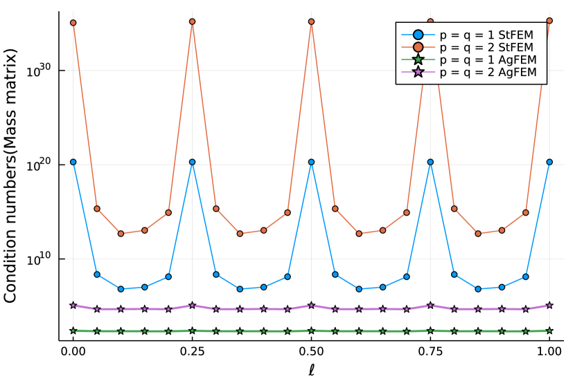
(a) Mass matrix

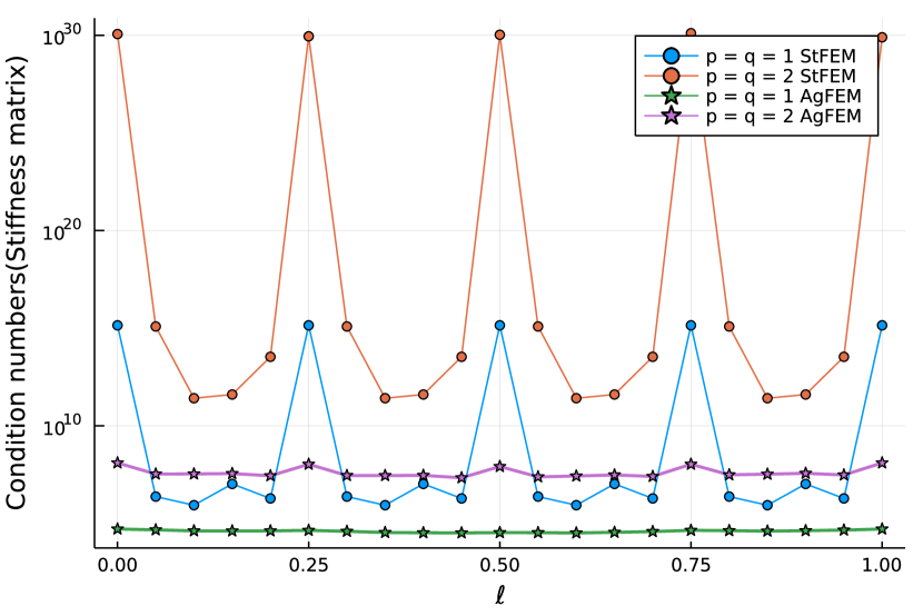
(b) Stiffness matrix

Figure 2. The figures depict the plots of condition numbers of the mass and stiffness matrices respectively against perturbation of the centre of the disk using AgFEM and StFEM for linear and quadratic polynomials in space and time.

The plot of condition numbers of the mass and stiffness matrices against the perturbation of the centre of the disk ($\ell$) is illustrated in Figure  2. We observe that the condition numbers using AgFEM are not affected by moving the position of the disk, i.e., it is robust with respect to the cut location, whereas there are huge fluctuations using StFEM. As the position of the disk changes, the cut locations change and some configurations of the geometry result in higher condition numbers using StFEM due to the small cut cell problem. The problem is more severe for quadratic StFEM in space-time, leading to almost singular matrices in some cases. On the other hand, the position of the geometry plays a negligible role in determining the condition numbers of the mass and stiffness matrices in the proposed space-time AgFEM.

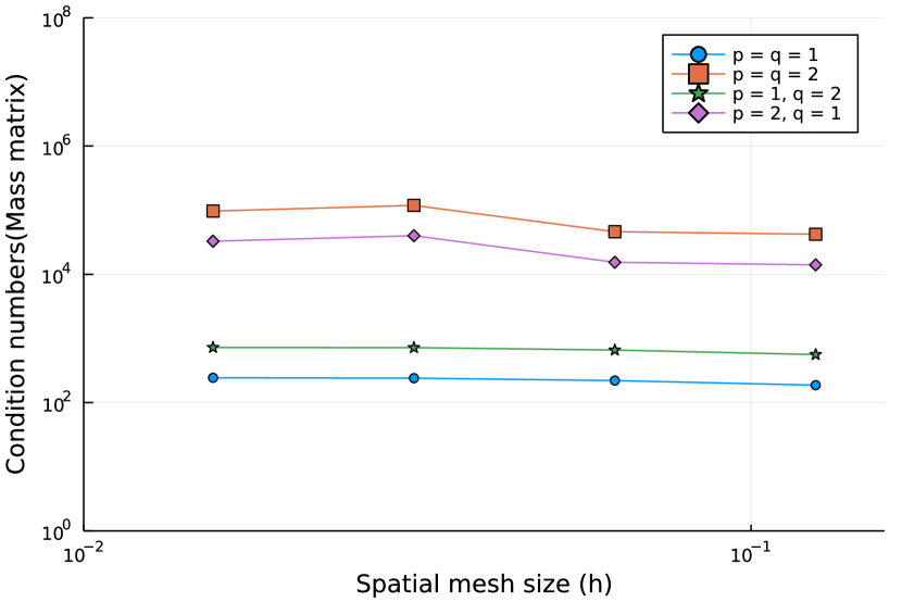
(a) Mass matrix

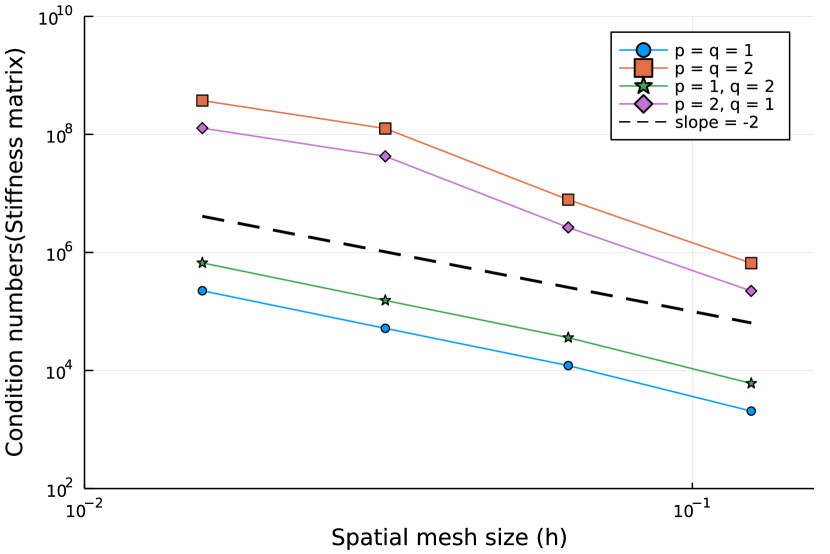
(b) Stiffness matrix

Figure 3. Plots of condition numbers of the mass and stiffness matrices against the spatial mesh size $h$ using AgFEM for a single time slab of size $\tau=h$.

In the next experiment we study the behaviour of condition numbers of the mass and stiffness matrices with respect to mesh refinement. We consider the moving geometry with the circular hole and spatial background meshes of sizes $h=2^{-m},m=3,4,5,6$ and a single time slab of size $\tau=h$. The plot of condition numbers against the spatial mesh size $h$ using AgFEM is depicted in Figure 3. We observe that the condition numbers of the mass matrix are almost constant whereas the condition numbers of the stiffness matrix scale with $\mathcal{O}(h^{-2})$ using AgFEM, which is the expected ratio.

5.4. Convergence tests

This experiment shows the behaviour of the error with respect to mesh refinement. We consider a geometry with a moving square hole, spatial background meshes of sizes $h=2^{-m},m=3,4,5,6$ and a constant time step size $\tau=h$. Since the domain is polyhedral, the geometry is exactly represented. We plot the error in the accumulated DG norm against the mesh size choosing the value of the coercivity constant $c_{\mu}=1$ in Figure 4(a).

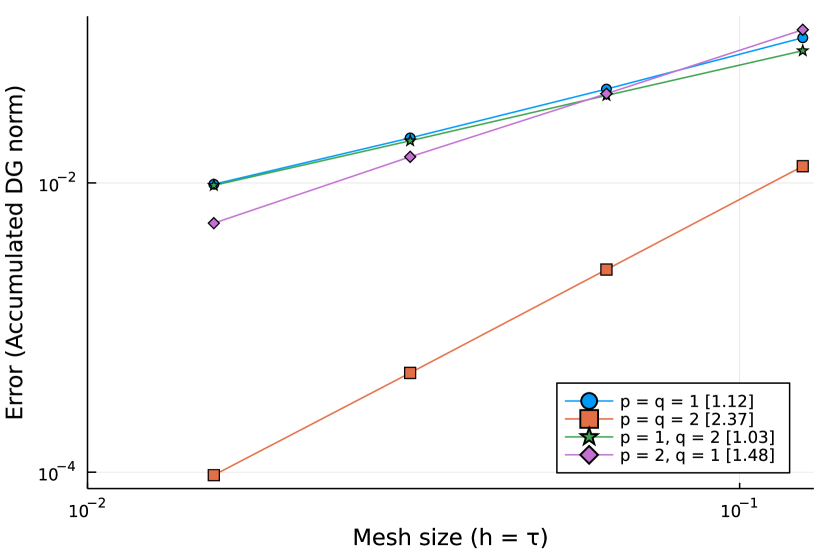
(a) Accumulated DG norm

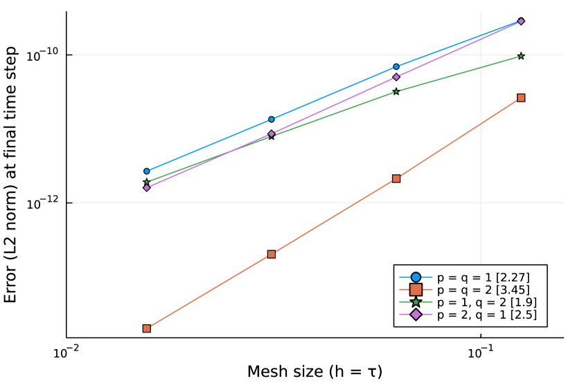
(b) $L^{2}(\Omega^{N})$ norm

Figure 4. The first figure illustrates the plot of total error in the accumulated DG norm (with constant $c_{\mu}=1$) against the mesh size ($h=\tau$) using AgFEM. The second figure depicts the plot of error in the $L^{2}$ norm at the final time step against the mesh size ($h=\tau$) using AgFEM

We observe that using AgFEM, when the ratio $h/\tau$ remains constant during refinement, the error converges with $\mathcal{O}(h^{s})$, where $s\doteq\min(p,q)$. This result is in agreement with (29).

In addition, with the same experimental setup the error in the $L^{2}(\Omega^{N})$ norm is computed and plotted against the mesh size in Figure 4(b). We observe higher convergence compared to the results using the accumulated DG norm. The error scales with $\mathcal{O}(h^{r})$, where $r\doteq\min(p+1,q+1)$.

5.5. An example with topology change

This last example studies the embedded space-time method in a more challenging geometrical configuration consisting of a time-dependent domain that undergoes topological changes. The example is taken from [34, 30] where it is also considered to characterise the performance of other embedded FE methods for time-evolving domains. The problem geometry is the union of two disks that travel with opposite velocities and eventually intersect (see Figure 5). We describe the disks with the level-set functions,

$$\phi_{1}(\boldsymbol{x},t)=|\boldsymbol{x}-(0,t-3/4)^{\mathrm{T}}|-0.5,$$

$$\phi_{2}(\boldsymbol{x},t)=|\boldsymbol{x}-(0,3/4-t)^{\mathrm{T}}|-0.5,$$

$|\boldsymbol{v}|$ being the algebraic 2-norm of a vector $\boldsymbol{v}$. From these level-set functions, the time-dependent problem geometry is defined as

$$\Omega(t)=\{\boldsymbol{x}\in\mathbb{R}^{2}:\ \min(\phi_{1}(\boldsymbol{x},t),\phi_{2}(\boldsymbol{x},t))<0\}\text{ for }t\in[0,T],$$

where the minimum operator is used to define the level-set function that describes the union of the two disks. The final time is selected as $T=3/2$ so that the initial and final geometry coincide, namely $\Omega(0)=\Omega(T)$. The geometry is implicitly defined via a level-set function that is linearly approximated.

$-1$      $1$

$t=0$

$t=.2$

$t=.375$

$t=.55$

$t=.75$

$t=.95$

$t=1.125$

$t=1.3$

$T=1.5$

Figure 5. Numerical solution of the example in Section 5.5 at nine selected time instants for a discretisation of $60\times 121$ spatial cells and $60$ time slabs.

On $\Omega(t)$, we solve the advection-diffusion equation $\partial_{t}u+\boldsymbol{w}\cdot\nabla u-\mu\Delta u=0$ with homogeneous Neumann boundary conditions, $\boldsymbol{n_{x}}\cdot\nabla u=0$, and the initial condition $u(x,y,0)=\mathrm{sign}(y)$. The advection velocity field is given by

$$\boldsymbol{w}(x,y,t)=\left\{\begin{aligned} (0,1)^{\mathrm{T}}\quad\text{if }y>0\text{ and }t\leq T/2\text{ or }y<0\text{ and }t>T/2\\ (0,-1)^{\mathrm{T}}\quad\text{if }y\leq 0\text{ and }t\leq T/2\text{ or }y\leq 0\text{ and }t>T/2\ \end{aligned}\right..$$

As in [34, 30], we take $\mu=0.1$. For this value of the diffusion coefficient, the problem is diffusion-dominated and it can be solved with the numerical scheme presented in previous sections without any further stabilisation technique. We only need to introduce the advection term in the weak form in the obvious way. Adding numerical stabilisation for the advection term (e.g., SUPG) would be also possible, but we want to use a numerical scheme as close as possible as the one analysed in previous sections, as permitted by the diffusion-dominated nature of this example.

As the advection velocity coincides with the motion of the disks $\boldsymbol{w}\cdot\boldsymbol{n_{x}}+n_{t}=0$ holds on the boundary of the domain and the problem is well-posed, as discussed in Sec. 3.1.

For the numerical discretisation, we consider a Cartesian mesh of the artificial domain $\Omega_{art}\doteq(-0.6,0.6)\times(-1.35,1.35)$ with two different resolutions consisting of $60\times 121$ cells. We deliberately use an odd number of cells in the $y$-direction so that the first contact of the two disks happens within a single cut cell. Otherwise, the first contact would take place at a cell boundary, which is an unrealistically simple particular case. The temporal discretisation is fixed to $60$ time slabs.

Figure 5 shows the obtained solution. The constant initial condition at the two disks is transported by the advection field with the same velocity as the motion of the disks themselves. At the contact event, a topologically new domain is created and diffusion starts to take place due to a sudden formation of a concentration gradient. A detailed view of the contact zone is given in Figure 6. Note that the numerical scheme is able to capture the sharp concentration gradient that takes place at the contact point without introducing numerical artefacts. In contrast to the results reported in [34, 30], we do not see any spurious diffusion starting before the time of first contact even though there is only a single full cell between the two disks at the time slab right before contact (see Figure 6(a)). For our formulation, diffusion would appear only when the disks get in touch (if aggregated cut cells are duplicated when they have disconnected regions). This is in contrast to the results in [34] for which the diffusion might start before, even with several layers of full cells between the disks, depending on the time step size. We can conclude that our numerical scheme is able to properly handle the topological change in this example. Similar results can be achieved for the weak AgFEM method proposed in Sec. 3.3.

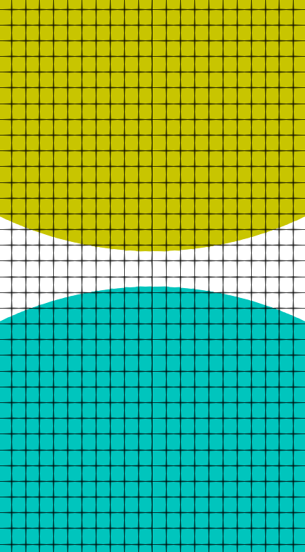
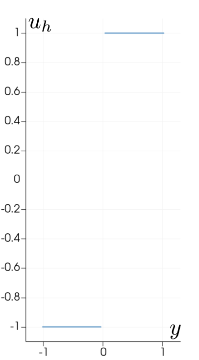
(a) $t=.225$

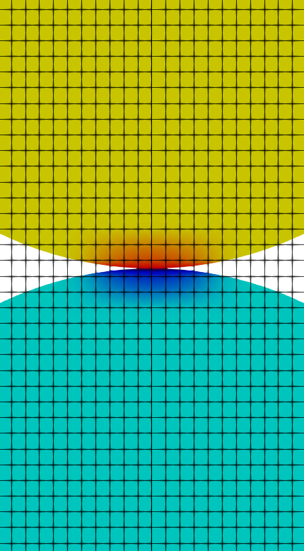
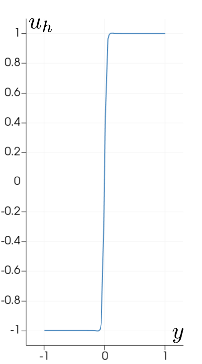
(b) $t=.25$

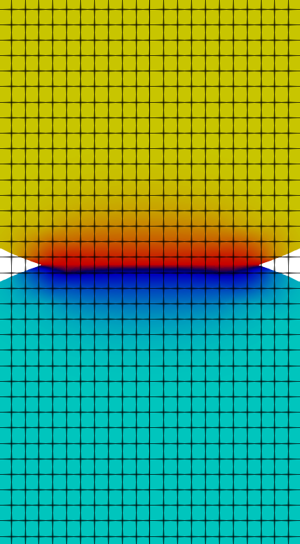
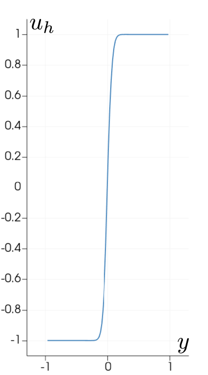
(c) $t=.275$

Figure 6. Detailed view of the contact zone for the last time step before contact, the time step when the contact takes place, and the next step after contact. The right hand side of each sub-figure shows the numerical solution $u_{h}$ restricted to the vertical line $x=0$ (the symmetry axis of the problem). The first contact point coincides with $(0,0)^{\mathrm{T}}$. The colour bar of this figure is the same as in Figure 5.

6. Conclusions

In this work, we have proposed a novel space-time unfitted FE technique to solve time-dependent partial differential equations. The use of a variational space-time formulation is proposed to approximate problems with moving domains or interfaces. In order to circumvent the lack of robustness of these methods to cut locations, we have extended AgFEM to space-time.

AgFE spaces are defined as the image of a discrete extension operator that constrains ill-posed DOFs with well-posed DOFs. Using a slab-wise time-constant cell aggregation algorithm, we have defined a discrete extension operator only in space at any time value. The image of this operator is a slab-wise AgFE space that can be expressed as a tensor-product of spatial and temporal spaces. Due to the definition of well-posedness of space-time cells, this discrete extension operator provides the required robustness with respect to the small cut cell problem.

We have carried out the numerical analysis (stability and convergence) of this proposed method for the numerical approximation of the heat equation on moving domains. However, other problems, e.g., convection-diffusion-reaction or even incompressible fluid problems using stabilisation techniques, could be analysed using similar arguments. Exploiting the tensor-product structure of the space, we can prove optimal error estimates. In addition, we have carried out a set of numerical experiments that support the theoretical results for the heat equation and an interface mass transfer problem that involves the advection-diffusion equation. The method proves to be robust and accurate in all scenarios.

The present work can readily be applied to (parallel) locally refined $n$-tree meshes using the space discrete extension operator in [5]. The extension to adaptive mesh refinement in space and time (local time stepping) can be considered in the future.

References

- Badia and Verdugo [2020] S. Badia and F. Verdugo. Gridap: An extensible finite element toolbox in Julia. Journal of Open Source Software, 5(52):2520, Aug. 2020. doi:10.21105/joss.02520. URL https://doi.org/10.21105/joss.02520.
- Badia et al. [2018a] S. Badia, A. F. Martin, and F. Verdugo. Mixed aggregated finite element methods for the unfitted discretization of the Stokes problem. SIAM Journal on Scientific Computing, 40(6):B1541–B1576, Jan. 2018a. doi:10.1137/18m1185624. URL https://doi.org/10.1137/18m1185624.
- Badia et al. [2018b] S. Badia, F. Verdugo, and A. F. Martín. The aggregated unfitted finite element method for elliptic problems. Computer Methods in Applied Mechanics and Engineering, 336:533–553, July 2018b. doi:10.1016/j.cma.2018.03.022. URL https://doi.org/10.1016/j.cma.2018.03.022.
- Badia et al. [2021a] S. Badia, J. Hampton, and J. Principe. Embedded multilevel Monte Carlo for uncertainty quantification in random domains. International Journal for Uncertainty Quantification, 11(1):119–142, 2021a. doi:10.1615/int.j.uncertaintyquantification.2021032984. URL https://doi.org/10.1615/int.j.uncertaintyquantification.2021032984.
- Badia et al. [2021b] S. Badia, A. F. Martín, E. Neiva, and F. Verdugo. The aggregated unfitted finite element method on parallel tree-based adaptive meshes. SIAM Journal on Scientific Computing, 43(3):C203–C234, Jan. 2021b. doi:10.1137/20m1344512. URL https://doi.org/10.1137/20m1344512.
- Badia et al. [2022a] S. Badia, P. A. Martorell, and F. Verdugo. Geometrical discretisations for unfitted finite elements on explicit boundary representations. Journal of Computational Physics, 460:111162, July 2022a. doi:10.1016/j.jcp.2022.111162. URL https://doi.org/10.1016/j.jcp.2022.111162.
- Badia et al. [2022b] S. Badia, E. Neiva, and F. Verdugo. Linking ghost penalty and aggregated unfitted methods. Computer Methods in Applied Mechanics and Engineering, 388:114232, Jan. 2022b. doi:10.1016/j.cma.2021.114232. URL https://doi.org/10.1016/j.cma.2021.114232.
- Badia et al. [2022c] S. Badia, E. Neiva, and F. Verdugo. Robust high-order unfitted finite elements by interpolation-based discrete extension, 2022c. URL https://arxiv.org/abs/2201.06632.
- Bassi et al. [2012] F. Bassi, L. Botti, A. Colombo, and S. Rebay. Agglomeration based discontinuous Galerkin discretization of the Euler and Navier–Stokes equations. Computers & Fluids, 61:77–85, May 2012. doi:10.1016/j.compfluid.2011.11.002. URL https://doi.org/10.1016/j.compfluid.2011.11.002.
- Beau et al. [1993] G. L. Beau, S. Ray, S. Aliabadi, and T. Tezduyar. SUPG finite element computation of compressible flows with the entropy and conservation variables formulations. Computer Methods in Applied Mechanics and Engineering, 104(3):397–422, May 1993. doi:10.1016/0045-7825(93)90033-t. URL https://doi.org/10.1016/0045-7825(93)90033-t.
- Bezanson et al. [2017] J. Bezanson, A. Edelman, S. Karpinski, and V. B. Shah. Julia: A fresh approach to numerical computing. SIAM Review, 59(1):65–98, Jan. 2017. doi:10.1137/141000671. URL https://doi.org/10.1137/141000671.
- Brenner and Scott [2008] S. C. Brenner and L. R. Scott. The Mathematical Theory of Finite Element Methods. Springer New York, 2008. doi:10.1007/978-0-387-75934-0. URL https://doi.org/10.1007/978-0-387-75934-0.
- Burman [2010] E. Burman. Ghost penalty. Comptes Rendus Mathematique, 348(21-22):1217–1220, Nov. 2010. doi:10.1016/j.crma.2010.10.006. URL https://doi.org/10.1016/j.crma.2010.10.006.
- Burman and Fernández [2014] E. Burman and M. A. Fernández. An unfitted Nitsche method for incompressible fluid–structure interaction using overlapping meshes. Computer Methods in Applied Mechanics and Engineering, 279:497–514, Sept. 2014. doi:10.1016/j.cma.2014.07.007. URL https://doi.org/10.1016/j.cma.2014.07.007.
- Burman et al. [2014] E. Burman, S. Claus, P. Hansbo, M. G. Larson, and A. Massing. CutFEM: Discretizing geometry and partial differential equations. International Journal for Numerical Methods in Engineering, 104(7):472–501, Dec. 2014. doi:10.1002/nme.4823. URL https://doi.org/10.1002/nme.4823.
- Burman et al. [2020] E. Burman, P. Hansbo, and M. G. Larson. Explicit time stepping for the wave equation using CutFEM with discrete extension, 2020. URL https://arxiv.org/abs/2011.05386.
- Burman et al. [2021] E. Burman, M. Cicuttin, G. Delay, and A. Ern. An unfitted hybrid high-order method with cell agglomeration for elliptic interface problems. SIAM Journal on Scientific Computing, 43(2):A859–A882, Jan. 2021. doi:10.1137/19m1285901. URL https://doi.org/10.1137/19m1285901.
- Carraturo et al. [2020] M. Carraturo, J. Jomo, S. Kollmannsberger, A. Reali, F. Auricchio, and E. Rank. Modeling and experimental validation of an immersed thermo-mechanical part-scale analysis for laser powder bed fusion processes. Additive Manufacturing, 36:101498, Dec. 2020. doi:10.1016/j.addma.2020.101498. URL https://doi.org/10.1016/j.addma.2020.101498.
- Chrysafinos and Walkington [2006] K. Chrysafinos and N. J. Walkington. Error estimates for the discontinuous Galerkin methods for parabolic equations. SIAM Journal on Numerical Analysis, 44(1):349–366, Jan. 2006. doi:10.1137/030602289. URL https://doi.org/10.1137/030602289.
- Claus and Kerfriden [2019] S. Claus and P. Kerfriden. A CutFEM method for two-phase flow problems. Computer Methods in Applied Mechanics and Engineering, 348:185–206, May 2019. doi:10.1016/j.cma.2019.01.009. URL https://doi.org/10.1016/j.cma.2019.01.009.
- Dekker et al. [2019] R. Dekker, F. Meer, J. Maljaars, and L. Sluys. A cohesive XFEM model for simulating fatigue crack growth under mixed-mode loading and overloading. International Journal for Numerical Methods in Engineering, 118(10):561–577, Feb. 2019. doi:10.1002/nme.6026. URL https://doi.org/10.1002/nme.6026.
- Donea et al. [1982] J. Donea, S. Giuliani, and J. Halleux. An arbitrary Lagrangian-Eulerian finite element method for transient dynamic fluid-structure interactions. Computer Methods in Applied Mechanics and Engineering, 33(1-3):689–723, Sept. 1982. doi:10.1016/0045-7825(82)90128-1. URL https://doi.org/10.1016/0045-7825(82)90128-1.
- Engwer and Heimann [2012] C. Engwer and F. Heimann. Dune-UDG: A cut-cell framework for unfitted discontinuous Galerkin methods. In Advances in DUNE, pages 89–100. Springer Berlin Heidelberg, 2012. doi:10.1007/978-3-642-28589-9_7. URL https://doi.org/10.1007/978-3-642-28589-9_7.
- Ern and Guermond [2004] A. Ern and J.-L. Guermond. Theory and Practice of Finite Elements. Springer New York, 2004. doi:10.1007/978-1-4757-4355-5. URL https://doi.org/10.1007/978-1-4757-4355-5.
- Formaggia et al. [2021] L. Formaggia, F. Gatti, and S. Zonca. An XFEM/DG approach for fluid-structure interaction problems with contact. Applications of Mathematics, 66(2):183–211, Jan. 2021. doi:10.21136/am.2021.0310-19. URL https://doi.org/10.21136/am.2021.0310-19.
- Giovanardi et al. [2017] B. Giovanardi, L. Formaggia, A. Scotti, and P. Zunino. Unfitted FEM for modelling the interaction of multiple fractures in a poroelastic medium. In Lecture Notes in Computational Science and Engineering, pages 331–352. Springer International Publishing, 2017. doi:10.1007/978-3-319-71431-8_11. URL https://doi.org/10.1007/978-3-319-71431-8_11.
- Gross and Reusken [2011] S. Gross and A. Reusken. Numerical Methods for Two-phase Incompressible Flows. Springer Berlin Heidelberg, 2011. doi:10.1007/978-3-642-19686-7. URL https://doi.org/10.1007/978-3-642-19686-7.
- Guzmán et al. [2017] J. Guzmán, M. A. Sánchez, and M. Sarkis. A finite element method for high-contrast interface problems with error estimates independent of contrast. Journal of Scientific Computing, 73(1):330–365, Mar. 2017. doi:10.1007/s10915-017-0415-x. URL https://doi.org/10.1007/s10915-017-0415-x.
- Heimann [2021] F. Heimann. On discontinuous- and continuous-in-time unfitted space-time methods for PDEs on moving domains, 2021. URL https://data.goettingen-research-online.de/citation?persistentId=doi:10.25625/CDCMYT.
- Heimann et al. [2022] F. Heimann, C. Lehrenfeld, and J. Preuß. Geometrically higher order unfitted space-time methods for PDEs on moving domains, 2022. URL https://arxiv.org/abs/2202.02216.
- Kummer [2016] F. Kummer. Extended discontinuous Galerkin methods for two-phase flows: the spatial discretization. International Journal for Numerical Methods in Engineering, 109(2):259–289, June 2016. doi:10.1002/nme.5288. URL https://doi.org/10.1002/nme.5288.
- Lehrenfeld [2015] C. Lehrenfeld. On a Space-Time Extended Finite Element Method for the Solution of a Class of Two-Phase Mass Transport Problems. Dissertation, RWTH Aachen University, Aachen, 2015. URL https://publications.rwth-aachen.de/record/462743. Aachen, Techn. Hochsch., Diss., 2015.
- Lehrenfeld [2016] C. Lehrenfeld. High order unfitted finite element methods on level set domains using isoparametric mappings. Computer Methods in Applied Mechanics and Engineering, 300:716–733, Mar. 2016. doi:10.1016/j.cma.2015.12.005. URL https://doi.org/10.1016/j.cma.2015.12.005.
- Lehrenfeld and Olshanskii [2019] C. Lehrenfeld and M. Olshanskii. An Eulerian finite element method for PDEs in time-dependent domains. ESAIM: Mathematical Modelling and Numerical Analysis, 53(2):585–614, Mar. 2019. doi:10.1051/m2an/2018068. URL https://doi.org/10.1051/m2an/2018068.
- Lehrenfeld and Reusken [2013] C. Lehrenfeld and A. Reusken. Analysis of a nitsche XFEM-DG discretization for a class of two-phase mass transport problems. SIAM Journal on Numerical Analysis, 51(2):958–983, Jan. 2013. doi:10.1137/120875260. URL https://doi.org/10.1137/120875260.
- Li et al. [2019] K. Li, N. M. Atallah, G. A. Main, and G. Scovazzi. The shifted interface method: A flexible approach to embedded interface computations. International Journal for Numerical Methods in Engineering, 121(3):492–518, Oct. 2019. doi:10.1002/nme.6231. URL https://doi.org/10.1002/nme.6231.
- Lundholm [2015] C. Lundholm. A space-time cut finite element method for a time-dependent parabolic model problem. Master’s thesis, 2015.
- Lundholm [2021] C. Lundholm. Cut Finite Element Methods on Overlapping Meshes: Analysis and Applications. Chalmers Tekniska Hogskola (Sweden), 2021.
- Martin et al. [2022] A. F. Martin, F. Verdugo, S. Badia, and O. Colomés. gridap/GridapDistributed.jl: v0.2.5, Feb. 2022. URL https://doi.org/10.5281/zenodo.6076710.
- Neiva and Badia [2021] E. Neiva and S. Badia. Robust and scalable h-adaptive aggregated unfitted finite elements for interface elliptic problems. Computer Methods in Applied Mechanics and Engineering, 380:113769, July 2021. doi:10.1016/j.cma.2021.113769. URL https://doi.org/10.1016/j.cma.2021.113769.
- Neiva et al. [2020] E. Neiva, M. Chiumenti, M. Cervera, E. Salsi, G. Piscopo, S. Badia, A. F. Martín, Z. Chen, C. Lee, and C. Davies. Numerical modelling of heat transfer and experimental validation in powder-bed fusion with the virtual domain approximation. Finite Elements in Analysis and Design, 168:103343, Jan. 2020. doi:10.1016/j.finel.2019.103343. URL https://doi.org/10.1016/j.finel.2019.103343.
- Nitsche [1971] J. Nitsche. Über ein Variationsprinzip zur Lösung von Dirichlet-Problemen bei Verwendung von Teilräumen, die keinen Randbedingungen unterworfen sind. Abhandlungen aus dem Mathematischen Seminar der Universität Hamburg, 36(1):9–15, July 1971. doi:10.1007/bf02995904. URL https://doi.org/10.1007/bf02995904.
- Nobile and Formaggia [1999] F. Nobile and L. Formaggia. A stability analysis for the arbitrary Lagrangian Eulerian formulation with finite elements. East-West Journal of Numerical Mathematics, 7(2):105–132, 1999.
- Preuß [2021] J. Preuß. "Higher order unfitted isoparametric space-time FEM on moving domains" (master’s thesis), 2021. URL https://data.goettingen-research-online.de/citation?persistentId=doi:10.25625/UACWXS.
- Reusken [2014] A. Reusken. Analysis of trace finite element methods for surface partial differential equations. IMA Journal of Numerical Analysis, 35(4):1568–1590, Oct. 2014. doi:10.1093/imanum/dru047. URL https://doi.org/10.1093/imanum/dru047.
- Saito [2020] N. Saito. Variational analysis of the discontinuous Galerkin time-stepping method for parabolic equations. IMA Journal of Numerical Analysis, 41(2):1267–1292, May 2020. doi:10.1093/imanum/draa017. URL https://doi.org/10.1093/imanum/draa017.
- Saye [2017] R. Saye. Implicit mesh discontinuous Galerkin methods and interfacial gauge methods for high-order accurate interface dynamics, with applications to surface tension dynamics, rigid body fluid–structure interaction, and free surface flow: Part I. Journal of Computational Physics, 344:647–682, Sept. 2017. doi:10.1016/j.jcp.2017.04.076. URL https://doi.org/10.1016/j.jcp.2017.04.076.
- Schott et al. [2019] B. Schott, C. Ager, and W. A. Wall. Monolithic cut finite element–based approaches for fluid-structure interaction. International Journal for Numerical Methods in Engineering, 119(8):757–796, Apr. 2019. doi:10.1002/nme.6072. URL https://doi.org/10.1002/nme.6072.
- Smears [2016] I. Smears. Robust and efficient preconditioners for the discontinuous Galerkin time-stepping method. IMA Journal of Numerical Analysis, page drw050, Oct. 2016. doi:10.1093/imanum/drw050. URL https://doi.org/10.1093/imanum/drw050.
- Sudirham et al. [2006] J. Sudirham, J. van der Vegt, and R. van Damme. Space–time discontinuous Galerkin method for advection–diffusion problems on time-dependent domains. Applied Numerical Mathematics, 56(12):1491–1518, Dec. 2006. doi:10.1016/j.apnum.2005.11.003. URL https://doi.org/10.1016/j.apnum.2005.11.003.
- Tezduyar et al. [2006] T. E. Tezduyar, S. Sathe, R. Keedy, and K. Stein. Space–time finite element techniques for computation of fluid–structure interactions. Computer Methods in Applied Mechanics and Engineering, 195(17-18):2002–2027, Mar. 2006. doi:10.1016/j.cma.2004.09.014. URL https://doi.org/10.1016/j.cma.2004.09.014.
- [52] V. Thomée. The discontinuous Galerkin time stepping method. In Galerkin Finite Element Methods for Parabolic Problems, pages 203–230. Springer Berlin Heidelberg. doi:10.1007/3-540-33122-0_12. URL https://doi.org/10.1007/3-540-33122-0_12.
- Thompson and Pinsky [1996] L. L. Thompson and P. M. Pinsky. A space-time finite element method for structural acoustics in infinite domains part 1: Formulation, stability and convergence. Computer Methods in Applied Mechanics and Engineering, 132(3-4):195–227, June 1996. doi:10.1016/0045-7825(95)00955-8. URL https://doi.org/10.1016/0045-7825(95)00955-8.
- Verdugo and Badia [2022] F. Verdugo and S. Badia. The software design of Gridap: A finite element package based on the Julia JIT compiler. Computer Physics Communications, 276:108341, July 2022. doi:10.1016/j.cpc.2022.108341. URL https://doi.org/10.1016/j.cpc.2022.108341.
- Verdugo et al. [2019] F. Verdugo, A. F. Martín, and S. Badia. Distributed-memory parallelization of the aggregated unfitted finite element method. Computer Methods in Applied Mechanics and Engineering, 357:112583, Dec. 2019. doi:10.1016/j.cma.2019.112583. URL https://doi.org/10.1016/j.cma.2019.112583.
- Verdugo et al. [2021] F. Verdugo, E. Neiva, and S. Badia. GridapEmbedded. Version 0.7., Oct. 2021. URL https://github.com/gridap/GridapEmbedded.jl. Available at https://github.com/gridap/GridapEmbedded.jl.
- Zahedi [2017] S. Zahedi. A space-time cut finite element method with quadrature in time. In Lecture Notes in Computational Science and Engineering, pages 281–306. Springer International Publishing, 2017. doi:10.1007/978-3-319-71431-8_9. URL https://doi.org/10.1007/978-3-319-71431-8_9.