The fractional volatility model and rough volatility

Abstract

The question of the volatility roughness is interpreted in the framework of a data-reconstructed fractional volatility model, where volatility is driven by fractional noise. Some examples are worked out and also, using Malliavin calculus for fractional processes, an option pricing equation and its solution are obtained.

Keywords: Stochastic volatility, Fractional noise, Rough volatility

1 The fractional volatility model

Some years ago, in collaboration with M. J. Oliveira [1], a program was started to reconstruct the market process from the data, using only minimal mathematical and theoretical prejudices. Consistency with the data was the main concern and only two general hypothesis were used, namely:

(H1) The log-price process $\log S_{t}$ belongs to a probability product space $\Omega\otimes\Omega^{{}^{\prime}}$ of which the first one, $\Omega$, is the Wiener space and the second, $\Omega^{{}^{\prime}}$, is a probability space to be reconstructed from the data. Denote by $\omega\in\Omega$ and $\omega^{{}^{\prime}}\in\Omega^{{}^{\prime}}$ the elements (sample paths) in $\Omega$ and $\Omega^{{}^{\prime}}$ and by $\mathcal{F}_{t}$ and $\mathcal{F}_{t}^{{}^{\prime}}$ the $\sigma-$algebras in $\Omega$ and $\Omega^{{}^{\prime}}$ generated by the processes up to $t$. Then, a particular realization of the log-price process would be denoted

$$\log S_{t}\left(\omega,\omega^{{}^{\prime}}\right)$$

This first hypothesis is really not limitative. Even if none of the non-trivial stochastic features of the log-price were captured by Brownian motion, that would simply mean that $S_{t}$ is a trivial function in $\Omega$.

(H2) The second hypothesis is stronger, although natural. It is assumed that for each fixed $\omega^{{}^{\prime}}$, $\log S_{t}\left(\bullet,\omega^{{}^{\prime}}\right)$ is a square integrable random variable in $\Omega$.

———

From the second hypothesis it follows that, for each fixed $\omega^{{}^{\prime}}$,

$$\begin{array}[]{lll}\frac{dS_{t}}{S_{t}}\left(\bullet,\omega^{{}^{\prime}}\right)&=&\mu_{t}\left(\bullet,\omega^{{}^{\prime}}\right)dt+\sigma_{t}\left(\bullet,\omega^{{}^{\prime}}\right)dB\left(t\right)\end{array}$$ (1)

where $\mu_{t}\left(\bullet,\omega^{{}^{\prime}}\right)$ and $\sigma_{t}\left(\bullet,\omega^{{}^{\prime}}\right)$ are well-defined processes in $\Omega$ (Theorem 1.1.3 in Ref.[2]). The process associated to the probability space $\Omega^{{}^{\prime}}$ was then inferred from the data and this data-reconstructed $\sigma_{t}$ process was called the induced volatility.

The scaling properties of the data-reconstructed induced volatility process were then carefully analyzed [1]. The conclusion was that the log-price, the volatility and the log-volatility are not self-similar processes and it is only after the log-volatility is integrated and the linear part extracted, that a self-similar process $R_{\sigma}\left(t\right)$ is obtained. This is an essential finding of the data-reconstructed model. That volatility is modeled by the finite differences of a self-similar process is an essential difference from other models that take into account the long-range correlation of the volatility. In some models [3] [4] [5] it is fractional Brownian motion (fBm) itself that drives the volatility, not a derivative of this process.

The simplest mathematical processes having these properties were identified and the following stochastic volatility model proposed

$$\begin{array}[]{lll}dS_{t}&=&\mu S_{t}dt+\sigma_{t}S_{t}dB\left(t\right)\\ \log\sigma_{t}&=&\beta+\frac{k}{\delta}\left\{B_{H}\left(t\right)-B_{H}\left(t-\delta\right)\right\}\end{array}$$ (2)

This fractional volatility model (FVM) is the minimal model that is consistent both with the mathematical hypothesis H1 and H2 and the scaling properties of the data.

$\delta$ is the observation time scale (one day, for daily data). In this model the volatility is not driven by fractional Brownian motion but by fractional noise. For the volatility (at resolution $\delta$)

$$\sigma\left(t\right)=\theta e^{\frac{k}{\delta}\left\{B_{H}\left(t\right)-B_{H}\left(t-\delta\right)\right\}-\frac{1}{2}\left(\frac{k}{\delta}\right)^{2}\delta^{2H}}$$ (3)

the term $-\frac{1}{2}\left(\frac{k}{\delta}\right)^{2}\delta^{2H}$ insuring that $E\left(\sigma\left(t\right)\right)=\theta$. In (2) the constant $k$ measures the strength of the volatility randomness. In the $\delta\rightarrow 0$ limit the driving process would be the distribution-valued process $W_{H}$

$$W_{H}=\lim_{\delta\rightarrow 0}\frac{1}{\delta}\left(B_{H}\left(t\right)-B_{H}\left(t-\delta\right)\right)$$ (4)

Explicit expressions for the distribution of price returns were obtained [1] and one interesting feature was the fact that, once the parameters were obtained from daily data in one market, then the model was also consistent with high-frequency data in a different market by simply changing the time scale $\delta$. This seemed somewhat mysterious until comparison with agent based models [6] revealed that in business-as-usual days, the random fluctuations depend more on the limit order book price mechanism than on the individual actions of the market players.

Further study [7] revealed that the FVM model (2) is arbitrage free. Furthermore, when the two sources of randomness (in $B\left(t\right)$ and $B_{H}\left(t\right)$) are related by an integral representation for $B_{H}\left(t\right)$ the market is also complete.

2 Rough volatility

Some time ago Gatheral and collaborators [10], working in the context of the Comte-Renault model [3], suggested, by the analysis of the roughness of volatility data, a value $H<\frac{1}{2}$ for the Hurst index. In a fractional Brownian motion process the Hurst index characterizes both the roughness and the correlation or anticorrelation of the process. Hence, if the volatility is driven by fractional Brownian motion, a Hurst index smaller than $\frac{1}{2}$ would seem to contradict the market long-range dependent volatility (volatility clustering) [11] [12]. The way the realized volatility is measured at high frequency has however been criticized by several authors [13] [14] [15] suggesting that the origin of the roughness lies in the microstructure noise [16] rather than on the actual volatility process.

However there is no real contradiction in the framework of the fractional volatility model (2) because there the volatility is driven by fractional noise (fN), not by fractional Brownian motion (fBm). Fig.1 compares a simulated path of $10000$ steps of fBm at $H=0.8$ with the corresponding one-step fractional noise ($B_{H}\left(t+1\right)-B_{H}\left(t\right)$).

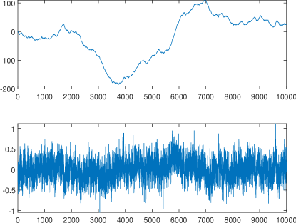
Figure 1: Fractional Brownian motion at $H=0.8$ and the corresponding one-step fractional noise

One sees that the apparent roughness of the fractional noise mimics fBm at $H\simeq 0.1$. Therefore, using the hypothesis, as in Comte and Renault [3], that it is fBm that drives volatility, one obtains the wrong Hurst index. What the data analysis performed in [1] implies is that, only when log-volatility is integrated and the linear part extracted, is a self-similar process $R_{\sigma}\left(t\right)$ obtained. Hence, long-range dependence and self-similarity are a property of integrated log-volatility, not of volatility itself.

As a check I have picked up some volatility data [17] and performed the same analysis as in [1]. The data that was analyzed was one-day volatility $\sigma\left(t\right)$ for the indexes DAX, Russel 2000, S&P500 and EURO STOXX 50 for the period 20/05/2021 to 22/05/2022 (Fig.2), as well as 6 minute data for S&P500 for the period 24/11/2021 to 24/05/2022.

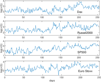
Figure 2: One-day volatility data for 4 indexes (May 2021-May 2022)

Fig.3 displays the results for the DAX index.

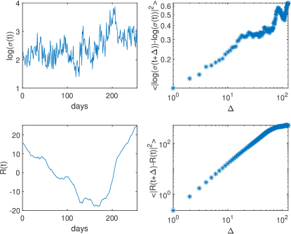
Figure 3: The fractional volatility analysis for the DAX index

The upper left panel displays $\log\sigma\left(t\right)$. Then, if this quantity were to follow fractional Brownian motion, as some authors have assumed, one would expect

$$\mathbb{E}\left\{\left(\log\sigma\left(t+\Delta\right)-\log\sigma\left(t\right)\right)^{2}\right\}\sim\Delta^{2H}$$

The upper right panel of Fig.3 clearly suggests that this is a bad hypothesis. In the figure $\left\langle\bullet\right\rangle$ stands for the empirical average, an empirical proxy for the expectation value. Next, I have formed the integrated log-volatility and after the extraction of the linear part $\beta t$ one obtains the process $R\left(t\right)$ (in the lower left panel)

$$\sum_{n=0}^{t/\delta}\log\sigma\left(n\delta\right)=\beta t+R\left(t\right)$$

Computing $\left\langle\left(R\left(t+\Delta\right)-R\left(t\right)\right)^{2}\right\rangle\approx\mathbb{E}\left\{\left(R\left(t+\Delta\right)-R\left(t\right)\right)^{2}\right\}$ one concludes (see the lower right panel of Fig.3) that

$$\mathbb{E}\left\{\left(R\left(t+\Delta\right)-R\left(t\right)\right)^{2}\right\}\sim\Delta^{2H}$$

and the identification of $R\left(t\right)$ with fractional Brownian motion is a reasonable hypothesis. Hence

$$\log\sigma\left(t\right)=\beta+\frac{k}{\delta}\left\{B_{H}\left(t\right)-B_{H}\left(t-\delta\right)\right\}$$

The following table shows the values of $\beta$ and $H$ that are obtained for the indexes that were analyzed

H $$\beta$$

SP500_1d 0.85 2.35

SP500_6min 0.86 2.77

Russel2000_1d 0.84 2.68

Euro_Stoxx_1d 0.84 2.59

DAX_1d 0.88 2.40

Fig.4 compares the DAX volatility data with a simulated sample path of the fractional volatility model (FVM) with the $H$ and $\beta$ values listed in the table. The model, having the same statistical properties as the data, might to be said to provide a ”perfect simulation” [18] of the data. However it must be pointed out, that perfect simulation in the statistical sense only means the same statistical properties, it is not ”perfect forecasting”. An attempt has been made in the past [19] to use the FVM to forecast volatility. The main conclusion was that although having the good statistical properties, FVM was not optimal as a forecasting device, because the market seemed to have, in addition to the stochastic terms in (2), a deterministic mean-reverting component, for example

$$\log\sigma\left(t\right)=\beta e^{\alpha\left(\beta-\log\sigma\left(t\right)\right)t}+\frac{k}{\delta}\left\{B_{H}\left(t\right)-B_{H}\left(t-\delta\right)\right\}$$

Such mean-reverting effect is in fact suggested by a close examination of the data plots and their comparison with the sample paths of the FVM.

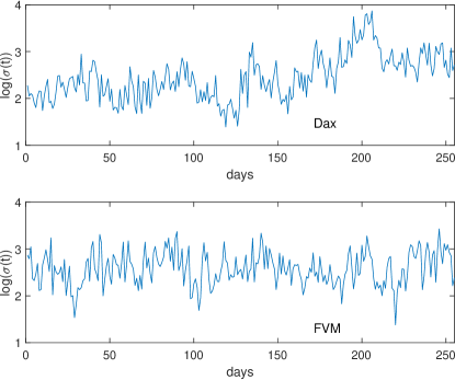
Figure 4: DAX volatility versus a corresponding fractional volatility model sample path

Finally, to the question of whether volatility is rough, the answer is yes, but only because it is driven by fractional noise with $H>\frac{1}{2}$.

One of the motivations for the development of reliable volatility models lies on the problem of option pricing and on corrections to Black-Scholes. In particular the rough volatility framework has also been used for option pricing [20]. In [1], using a simple-minded extension of the Hull-White [21] reasoning, an approximate formula was obtained with features similar to those observed in options data. Here a more rigorous derivation will be made, based on the mathematical framework that has been developed for the stochastic analysis of fractional processes.

3 Fractional stochastic analysis and option pricing

The idea of using fractional processes as a tool for modeling in Finance appeared at an early stage [22]. However, because it was pointed out [23] that markets based on $B_{H}\left(t\right)$ could have arbitrage, fractional Brownian motion (fBm) was not considered, for a while, as a promising tool for mathematical modeling in Finance. The arbitrage result in [23] is a consequence of using pathwise integration. With a different definition [8],

$$\int_{a}^{b}f\left(t,\omega\right)dB_{H}\left(t\right)=\lim_{\left|\Delta\right|\rightarrow 0}\sum_{k}f\left(t_{k},\omega\right)\diamond\left(B_{H}\left(t_{k+1}\right)-B_{H}\left(t_{k}\right)\right)$$

where $\Delta:a=t_{0}<t_{1}<\cdots<t_{n}=b$ is a partition of the interval $[a,b]$, $\left|\Delta\right|=\max_{0\leq k\leq n-1}\left(t_{k+1}-t_{k}\right)$ and $\diamond$ denotes the Wick product, the integral has zero expectation value and the arbitrage result is no longer true. This is, in fact, the most natural definition because it is the Wick product that is associated to integrals of Itô type, whereas the usual product is natural for integrals of Stratonovich type. An essentially equivalent approach constructs the stochastic integral through the divergence operator and Malliavin calculus [24]. In any case if fBm is included in the log return process [25] [26] it contradicts the empirical short autocorrelation of this process. The conclusion is that fractional processes are only relevant to drive the volatility, not the log-price itself.

A fully consistent stochastic calculus has now been developed for fractional Brownian motion [8] [9] [24] [25] [27] [28] [29] [30] and this is the setting that will be used here to derive an option pricing equation.

Because volatility is not a tradable security, a pure arbitrage argument cannot completely determine the fair price of an option. On the other hand, because of the fractional nature of the volatility process, volatility follows a stochastic process different from the one of the underlying security. Therefore, we cannot apply the reasoning [31] that leads to uniform coefficients of the form $\left(\mu_{i}-\lambda_{i}\sigma_{i}\right)$ in the first derivative terms of the option pricing equation. Hence, a first principles derivation, with clearly specified assumptions is required.

As in Black-Scholes [32] [33] form a portfolio

$$\Pi\left(t\right)=V\left(S,\sigma,t\right)-\Delta\left(S,\sigma,t\right)S_{t}$$ (5)

To compute the stochastic differential of $\Pi\left(t\right)$ one uses the Itô formula for the price process ($S_{t}$) and the fractional Itô formula [8] Namely, if $dX_{t}=c\left(t,\omega\right)dB_{H}\left(t\right)$ , then

$$df\left(t,X_{t}\right)=\frac{\partial f}{\partial t}dt+\frac{\partial f}{\partial X}dX_{t}+\frac{\partial^{2}f}{\partial X^{2}}c\left(t,\omega\right)D_{t}^{\phi}\left(X_{t}\right)$$

$D_{t}^{\phi}\left(X_{t}\right)$ being the $\phi-$Malliavin derivative corresponding to the $X_{t}-$ process, defined by

$$D_{f}^{\phi}X_{t}\left(\omega\right) = \lim_{\varepsilon\rightarrow 0}\frac{1}{\varepsilon}\left\{X\left(\omega+\varepsilon\int_{0}^{\bullet}ds\int_{0}^{\infty}\phi\left(s,u\right)f\left(u\right)du\right)-X\left(\omega\right)\right\}$$

$$= \int_{0}^{\infty}D_{u}^{\phi}\left(X_{t}\right)f\left(u\right)du$$

$\phi\left(s,u\right)$ being the kernel

$$\phi\left(s,u\right)=H\left(2H-1\right)\left|s-u\right|^{2H-2}$$

for $\frac{1}{2}<H<1$

Then from (2), choosing $\Delta\left(S,\sigma,t\right)=\frac{\partial V}{\partial S}$ one obtains

$$d\Pi\left(t\right) = \left\{\frac{\partial V}{\partial t}+\frac{1}{2}\frac{\partial^{2}V}{\partial S^{2}}\sigma^{2}S^{2}\right\}dt+\frac{\partial V}{\partial\left(\log\sigma\right)}\frac{k}{\delta}\left(dB_{H}\left(t\right)-dB_{H}\left(t-\delta\right)\right)$$

$$+\frac{\partial^{2}V}{\partial\left(\log\sigma\right)^{2}}\frac{k^{2}}{\delta^{2}}D_{t}^{\phi}\left(B_{H}\left(t\right)-B_{H}\left(t-\delta\right)\right)$$

and computing the Malliavin derivative

$$d\Pi\left(t\right) = \left\{\frac{\partial V}{\partial t}+\frac{1}{2}\frac{\partial^{2}V}{\partial S^{2}}\sigma^{2}S^{2}\right\}dt+\sigma\frac{\partial V}{\partial\sigma}\frac{k}{\delta}\left(dB_{H}\left(t\right)-dB_{H}\left(t-\delta\right)\right)$$ (6)

$$+\left(\sigma^{2}\frac{\partial^{2}V}{\partial\sigma^{2}}+\sigma\frac{\partial V}{\partial\sigma}\right)\frac{k^{2}}{\delta^{2}}H\delta^{2H-1}dt$$

In (6) one is still left with the stochastic term $\sigma\frac{\partial V}{\partial\sigma}\frac{k}{\delta}\left(dB_{H}\left(t\right)-dB_{H}\left(t-\delta\right)\right)$ and, because volatility is not a tradable security this term cannot be eliminated by a portfolio choice. Instead one identifies this term with a (deterministic) market price of volatility term $\nu\frac{k}{\delta}\sigma\frac{\partial V}{\partial\sigma}dt$ with $\nu>0$. Finally from $d\Pi\left(t\right)=r\Pi\left(t\right)dt$, $r$ being the risk-free return, one ends up with

$$\frac{\partial V}{\partial t}+rS\frac{\partial V}{\partial S}+\frac{\sigma^{2}S^{2}}{2}\frac{\partial^{2}V}{\partial S^{2}}+\frac{k}{\delta}\left(kH\delta^{2H-2}-\nu\right)\sigma\frac{\partial V}{\partial\sigma}+Hk^{2}\delta^{2H-3}\sigma^{2}\frac{\partial^{2}V}{\partial\sigma^{2}}=rV$$ (7)

as the general form of an option pricing equation consistent with the stochastic volatility model in (2).

One now obtains an integral representation for the solution of this equation with the change of variable

$$x=\log\frac{S}{K}$$ (8)

and passing to the two-dimensional Fourier transform

$$V\left(t,x,\sigma\right)=\int\int d\phi d\rho F\left(\phi,\rho,\sigma\right)e^{i\left(\phi t+\rho x\right)}$$ (9)

Then

$$Hk^{2}\delta^{2H-3}\sigma^{2}\frac{\partial^{2}F}{\partial\sigma^{2}}+\frac{k}{\delta}\left(kH\delta^{2H-2}-\nu\right)\sigma\frac{\partial F}{\partial\sigma}+\left(i\left(\phi+\rho r-\frac{\sigma^{2}\rho}{2}\right)-\frac{\sigma^{2}\rho^{2}}{2}-r\right)F=0$$ (10)

Defining new constants

$$\begin{array}[]{lll}\chi\left(\rho\right)&=&\frac{\nu}{2Hk\delta^{2H-2}}\\ \xi^{2}\left(\rho,\phi\right)&=&\chi^{2}\left(\rho\right)-\frac{r-i\left(\phi+\rho r\right)}{Hk^{2}\delta^{2H-3}}\\ \zeta^{2}\left(\rho\right)&=&-\frac{i\rho+\rho^{2}}{2Hk^{2}\delta^{2H-3}}\end{array}$$ (11)

and making the replacement

$$F\left(\sigma\right)=\sigma^{\chi}Z_{\xi}\left(\zeta\sigma\right)$$ (12)

Eq.(10) reduces to a standard Bessel equation. Therefore the solution of (7) is

$$V\left(t,x,\sigma\right)=\int\int d\rho d\phi e^{i\left(\phi t+\rho x\right)}\sigma^{\chi\left(\rho\right)}Z_{\xi(\rho,\phi)}\left(\zeta\left(\rho\right)\sigma\right)$$ (13)

$Z_{\xi}\left(\zeta\sigma\right)$ being a Bessel function. The Bessel function will be a linear combination

$$Z_{\xi}\left(\zeta\sigma\right)=c_{1}J_{\xi}\left(\zeta\sigma\right)+c_{2}N_{\xi}\left(\zeta\sigma\right)$$

of a Bessel function of first kind and a Neumann function, with coefficients $c_{1}$ and $c_{2}$ to be fixed by the boundary condition, which for call options is

$$V\left(T,x,\sigma\right)=\max\left(x,0\right)$$

Eq.(13) is an exact solution of the option pricing equation.

References

- [1] R. Vilela Mendes and M. J. Oliveira; A data-reconstructed fractional volatility model, http://www.economics-ejournal.org/economics/discussionpapers/2008-22.
- [2] D. Nualart; The Malliavin Calculus and Related Topics, Springer-Verlag, Berlin, 1995.
- [3] F. Comte and E. Renault; Long memory in continuous-time stochastic volatility models, Mathematical Finance 8 (1998) 291-323.
- [4] A. Gloter ad M. Hoffmann; Stochastic volatility and fractional Brownian motion, Stochastic Processes and their Applications 113 (2004) 143 – 172.
- [5] B. Djehiche and M. Eddahbi; Hedging options in market models modulated by fractional Brownian motion, Stochastic Analysis and Applications 19 (2001) 753-770.
- [6] R. Vilela Mendes; The fractional volatility model: An agent-based interpretation, Physica A 387 (2008) 3987–3994.
- [7] R. Vilela Mendes, M.J. Oliveira and A.M. Rodrigues; No-arbitrage, leverage and completeness in a fractional volatility model, Physica A 419 (2015) 470–478.
- [8] T. E. Duncan, Y. Hu and B. Pasik-Duncan; Stochastic calculus for fractional Brownian motion. I. Theory, SIAM J. Control Optim. 38 (2000) 582-612.
- [9] F. Biagini, B. Øksendal, a. Sulem and N. Wallner; An introduction to white-noise theory and Malliavin calculus for fractional Brownian motion, Proc. R. Soc. London A 460 (2004) 347-372.
- [10] J. Gatheral, T. Jaisson and M. Rosenbaum; Volatility is rough, Quantitative Finance 18 (2018) 933-949.
- [11] F. Breidt, N. Crato, and P. de Lima; The detection and estimation of long memory in stochastic volatility, Journal of Econometrics, 83 (1998) 325-348.
- [12] R. Cont; Empirical properties of asset returns: Stylized facts and statistical issues, Quantitative Finance 1 (2001) 1-14.
- [13] M. Fukasawa, T. Takabatake and R. Westphal; Is Volatility Rough ?, arXiv:1905.04852.
- [14] L. C. G. Rogers; Things we think we know, https://www.skokholm.co.uk/wp-content/uploads/2019/11/TWTWKpaper.pdf
- [15] R. Cont and P. Das; Rough volatility: fact or artefact?, arXiv:2203.13820.
- [16] A. Lahiri and R. Sen; Fractional Brownian markets with time-varying volatility and high-frequency data, Econometrics and Statistics 16 (2020) 91–107.
- [17] https://realized.oxford-man.ox.ac.uk./
- [18] A. Galves, E. Löcherbach and E. Orlandi; Perfect Simulation of Infinite Range Gibbs Measures and Coupling with Their Finite Range Approximations, J. Stat. Phys. 138 (2010) 476–495.
- [19] N. T. Martins; Previsão da volatilidade com um processo de ruído Browniano fraccionário subjacente, IST Master Thesis 2010, https://fenix.tecnico.ulisboa.pt/downloadFile/395142130230/Thesis.pdf
- [20] C. Bayer, P. K. Friz and J. Gatheral; Pricing under rough volatility, Quantitative Finance 16 (2016) 887-904.
- [21] J. C. Hull and A. White; The pricing of options on assets with stochastic volatility, Journal of Finance 42 (1987) 281-300.
- [22] B. B. Mandelbrot; Fractals and Scaling in Finance: Discontinuity, Concentration, Risk, Springer, New York 1997.
- [23] L. C. G. Rogers; Arbitrage with fractional Brownian motion, Math. Finance 7 (1997) 95-105.
- [24] E. Alòs and D. Nualart; Stochastic integration with respect to the fractional Brownian motion, Stochastics and Stochastics Reports 75 (2003) 129-152.
- [25] Y. Hu and B. Øksendal; Fractional white noise calculus and applications to finance, Infinite Dimensional Analysis, Quantum Probability and Related Topics 6 (2003) 1-32.
- [26] R. J. Elliott and L. Chan; Perpetual American options with fractional Brownian motion, Quantitative Finance 4 (2004) 123-128.
- [27] L. Decreusefond and A. S. Üstünel; Stochastic analysis of the fractional Brownian motion, Potential Analysis 10 (1998) 177-214.
- [28] Y. Hu; Heat equation with fractional white noise potentials, Applied Math. and Optimization 43 (2001) 221-243.
- [29] B. Øksendal and T. Zhang; Multiparameter fractional Brownian motion and quasi-linear stochastic differential equations, Stochastics and Stochastics Reports 71 (2001) 141-163.
- [30] E. Alòs, O. Mazet and D. Nualart; Stochastic calculus with respect to Gaussian processes, Ann. Probability 29 (2001) 766-801.
- [31] Y.-D. Lyuu; Financial Engineering and Computation, Chapter 15, Cambridge Univ. Press, Cambrige UK 2002.
- [32] F. Black and M. Scholes; The pricing of options and corporate liabilities, J. of Political Economy 81 (1973) 637-654.
- [33] R. C. Merton; Theory of rational option pricing, Bell J. Econ. Manag. Sci. 4 (1973) 141-183.