A weighted average distributed estimator for high dimensional parameter

Abstract

Distributed sparse learning for high dimensional parameters has attached vast attentions due to its wide application in prediction and classification in diverse fields of machine learning. Existing distributed sparse regression usually takes an average way to ensemble the local results produced by distributed machines, which enjoys low communication cost but is statistical inefficient. To address this problem, we proposed a new Weighted AVerage Estimate (WAVE) for high-dimensional regressions. The WAVE is a solution to a weighted least-square loss with an adaptive $L_{1}$ penalty, in which the $L_{1}$ penalty controls the sparsity and the weight promotes the statistical efficiency. It can not only achieve a balance between the statistical and communication efficiency, but also reach a faster rate than the average estimate with a very low communication cost, requiring the local machines delivering two vectors to the master merely. The consistency of parameter estimation and model selection is also provided, which guarantees the safety of using WAVE in the distributed system. The consistency also provides a way to make hypothisis testing on the parameter. Moreover, WAVE is robust to the heterogeneous distributed samples with varied mean and covariance across machines, which has been verified by the asymptotic normality under such conditions. Other competitors, however, do not own this property. The effectiveness of WAVE is further illustrated by extensive numerical studies and real data analyses.

Keywords: Distributed estimator, communication-efficient, statistical efficient, high-dimensional parameter, heterogeneous setting

1 Introduction

Distributed statistical learning for high-dimensional parameter has attached much attentions due to its wide application in various fields, which has been a central task in machine learning and statistical community. For example, in Internet security, an antivirus software may scan tens of thousands of keywords in millions of URLs per minute, resulting in huge datasets on the PC distributed in the internet. In the wireless communication, the sensing cognitive radios need to collaborate to estimate the radio-frequency power spectrum density, which can be seen as a parameter estimation of infinite dimension. Another example is the U.S. Airline dataset, which collects about 114 million observations about the flight information from 1987 to 2008, leading to a raw dataset over 12GB on a hardware . The aim is to learn a model as accurate as possible to predict the delayed status of a flight. In these applications, the main challenging in analyzing such kind of datasets is that the whole data set is hardly possible to be loaded into the memory of a single machine. Moreover, in some occasions, even one machine has enough capacity to store the data, solving a large-scale computation problem is still unaffordable in terms of time cost.

To address above concerns, distributed statistical learning (DSL) has been an efficient and popular approach to handle the huge dataset. DSL takes a master-and-workers architecture, in which the workers firstly learn local results, e.g., the summary statistics or the local models, in a parallel way and then deliver them to the master to ensemble a global one. Thanks to this simple structure, DSL has received increasing attention in recent years. Lee et al. (2017) devised a communication-efficient approach to distributed sparse regression in the high-dimensional setting via averaging debiased lasso estimators. Battey et al. (2018) studied distributed hypothesis testing and sparse parameter estimation in a unified likelihood-based framework. Jordan et al. (2019) built a communication-efficient distributed statistical inference via proposing a surrogate likelihood; Tang et al. (2020) proposed a distributed method for simultaneous inference of high-dimensional parameters in the generalized linear model. Zhu et al. (2021) developed a distributed least squares approximation method for a large family of regressions, e.g., linear regression, logistic regression and Cox’s model, on a distributed system. Tu et al. (2021) proposed a Byzantine-robust distributed sparse learning for the M-estimation. Lv and Lian (2022) considered a communication-efficient distributed learning algorithm for sparse partially linear models. For more literatures about DSL, one can refer to Lin and Xi (2011), Chang et al. (2017), Chang et al. (2017), Zhao et al. (2016), Huang and Huo (2019), Chen et al. (2019), Chen and Peng (2021), Tan et al. (2022), Huang et al. (2022) and the survey articles Chen and Xie (2014) and Gao et al. (2021).

Although various distributed learning schemes have been proposed recently for different models, little attention has been paid to distributed optimization for high-dimensional parameters with multiple structures, e.g., sparsity and huber-loss. Existing distributed learning methods for high-dimensional regression usually take the one-shot learning (OSL) method to save the communication cost, which requires only one-round communication between the master and workers. Among them, the simple average strategy (SAS) is the most popular OSL method since it is easy-to-implement and has a very low communication cost, only calling for several vectors from the workers, see for example Lee et al. (2017), Lv and Lian (2022) and etc. Algorithm SAS is effective in many scenarios, it is not statistical optimal unless the samples across machines are homogeneous. To improve this situation, some researchers proposed to pass more summary statistics, e.g., the information matrix, to the master. See Lin and Xi (2011), Huang and Huo (2019), Tang et al. (2020) and Zhu et al. (2021). Such a strategy enhances the statistical efficiency of the learning result but still faces the communication bottleneck in high-dimensional setting since the delivery of a large dimensional matrix is unaffordable. Besides OSL, another popular DSL method is the multiple-shot learning (MSL), which allows multiple rounds of communication between the master and workers. Consequently, the optimal statistical inference can be gradually achieved without many constraints on the number of workers. See for instance Chen et al. (2019) and Tu et al. (2021). However, the multiple-shot learning procedure would entail intolerable communication burden, especially for the high-dimensional problem. Besides, some MSL methods require not only local results but also raw data to ensemble the estimate, which is impossible in some occasions where the data privacy is in the first place.

The above discussions motivate us to develop a new distributed learning method for the high-dimensional regression. We propose a Weighted AVerage Estimate (WAVE) for the high-dimensional parameter, which is a solution to a weighted least-square loss with an adaptive $L_{1}$ penalty. Here, the weight is inversely proportional to the variance of local estimators and the $L_{1}$ penalty controls the sparsity of aggregated estimator. Compared to existing approaches, WAVE shed light on the following three aspects. First of all, it enjoys a low communication cost because it requires the workers delivering only two vectors to the master. Secondly, it is more statistical efficient than those methods taking the simple averaging strategy because of the addition of the weight. Last but not the least, it is shown that WAVE is still effective when the mean and covariance of the samples across workers are different. Actually, such a heterogeneous setting occurs in many real scenarios. For example, different labs could produce the experimental data with different variance even they perform a same experiment.

The contribution of this article is summarized as follows.

1. This paper proposes a new distributed sparse learning method, which can achieve a balance between the communication side and statistical efficient.

2. The newly proposed framework can be applied to a range of scenarios, including the linear model under the huber loss or the generalized linear model under the likelihood.

3. The theoretical analysis for WAVE, including the consistency of parameter estimation and variable selection, are provided. Particularly, the asymptotic normality under the heterogeneous setting is also established.

4. Extensive numerical studies and real data analyses are conducted to illustrate the merits of WAVE.

The organization of the paper is as follows. Section 2 gives the details of the methodological development. Section 3 provides some theoretical results to guarantee the reasonableness of the new method. Section 4 is the detailed algorithm and Section 5 presents some numerical evidences to examine the superiority of the new method over its competitors. Section 6 employs two real datasets to further illustrate the effectiveness of the new method. Section 7 makes a conclusion and discusses some further works. All the proof of this paper is postponed to the Appendix at the end of the paper.

2 Methodologies

Let $\bm{X}=\left(X_{1},X_{2},\ldots,X_{p}\right)^{\top}$ be a $p$-dimensional covariate and $Y$ be the response variable. The parameter of interest is defined as the minimizer of the following loss function,

$$\boldsymbol{\beta}^{*}=\mbox{argmin}_{\boldsymbol{\beta}\in\mathbb{R}^{p}}\mathbb{E}\left\{\mathcal{L}\left(Y,\boldsymbol{X}^{\top}\bm{\beta}\right)\right\},$$ (1)

where $\mathcal{L}(Y,z)$ is convex and twice-differentiable with respect to $z$, and vector $\boldsymbol{\beta}^{*}$ is assumed to be sparse, i.e. the number of nonzero entries in $\boldsymbol{\beta}^{*}$ is small compared with $p$. Framework (1) covers a wide range of models, the following are some typical examples:

(a)

Least square loss: $\mathcal{L}(Y,\bm{X}^{\top}\bm{\beta})=(Y-\bm{X}^{\top}\bm{\beta})^{2}$.

(b)

Huber loss: $\mathcal{L}(Y,\bm{X}^{\top}\bm{\beta})=h_{a}(Y-\bm{X}^{\top}\bm{\beta})$, where

$$h_{a}(x)=\left\{\begin{array}[]{ll}\frac{1}{2}x^{2},&\mbox{if~{}}|x|<a,\\ a|x|-\frac{1}{2}a^{2},&\mbox{otherwise},\end{array}\right.$$

(c)

Negative log-likelihood: $\mathcal{L}(Y,\bm{X}^{\top}\bm{\beta})=-\log\{\exp(Y\bm{X}^{\top}\bm{\beta})/(1+\exp(\bm{X}^{\top}\bm{\beta}))\}$ for logistic model and $\mathcal{L}(Y,\bm{X}^{\top}\bm{\beta})=-Y\bm{X}^{\top}\bm{\beta}+\exp(\bm{X}^{\top}\bm{\beta})$ for Poisson log-linear regression.

Suppose $(Y_{i},\bm{X}_{i}),i=1,\cdots,N$ are independent samples from $(Y,\bm{X})$. If there existed a “god-made” computer having the access to all samples, then we can estimate $\bm{\beta}^{*}$ as,

$$\widehat{\bm{\beta}}_{\lambda}=\operatorname{argmin}_{\boldsymbol{\beta}\in\mathbb{R}^{p}}\frac{1}{N}\sum_{i=1}^{N}\mathcal{L}\left(Y_{i},\boldsymbol{X}_{i}^{\top}\boldsymbol{\beta}\right)+\sum_{j=1}^{p}p_{j}(\lambda,\beta_{j})$$

where $p_{j}(\lambda,\beta_{j})$ is a penalty function to ensure the sparsity of $\bm{\beta}$. However, the master has no access to the raw data but only the permission to receive some summary statistics from the workers. In such a situation, we have to employ the divide-and-conquer strategy. Under the Master-Worker architecture, we suppose that the master can order the workers to execute the same instruction, although it cannot get the raw data from them.

Let $\mathcal{I}_{j}$ be the index set of the samples stored in $j$-th worker, then we propose to use the adaptive lasso method to estimate $\bm{\beta}$ in each worker:

$$\widehat{\bm{\beta}}_{j,\lambda_{nj}}=\mathop{\mbox{argmin}}_{\bm{\beta}}\frac{1}{2|\mathcal{I}_{j}|}\sum_{i\in\mathcal{I}_{j}}\mathcal{L}\left(Y_{i},\boldsymbol{X}_{i}^{\top}\boldsymbol{\beta}\right)+\lambda_{j}\sum_{k=1}^{p}\hat{\omega}_{k}|\beta_{k}|,$$ (2)

where $\hat{\omega}_{k}=1/|\hat{\beta}_{k}^{\mathrm{pre}}|^{\xi}$ for $\xi>0$, $\hat{\beta}_{k}^{\mathrm{pre}}$ is a pre-estimate of $\beta_{k}$; for example, we can set $\hat{\beta}_{j}^{\mathrm{pre}}$ as the lasso estimator. For the simplicity of notation, the super-script $\lambda_{n_{j}}$ in $\widehat{\bm{\beta}}_{j,\lambda_{n_{j}}}$ is neglected if there is no confusion. Theorem 1 in next section shows the consistency of $\widehat{\bm{\beta}}_{j}$ under some regular condition. Since $\widehat{\bm{\beta}}_{j}$ is unbiased, then we can aggregate them via two different ways, respectively, one is the simple average estimator, denoted as

$$\widehat{\bm{\beta}}^{AV}=\sum_{j=1}^{K}\alpha_{j}\widehat{\bm{\beta}}_{j}.$$ (3)

The other is the least-square estimator, denoted as

$$\widehat{\bm{\beta}}^{LS}=\left(\sum_{j=1}^{K}\alpha_{j}\widehat{\bm{\Sigma}}_{j}^{-1}\right)^{-1}\left(\sum_{j=1}^{K}\alpha_{j}\widehat{\bm{\Sigma}}_{j}^{-1}\widehat{\bm{\beta}}_{j}\right),$$ (4)

where $\widehat{\bm{\Sigma}}_{j}$ is the covariance matrix of $\widehat{\bm{\beta}}_{j}$. As discussed above, formula (3) is communication efficient but not accuracy enough. Formula (4) can gain more statistical efficiency but requires each worker to deliver at least $p^{2}-p/2$ elements to the master, which is unbearable when $p$ is large. To achieve a balance between the statistical and communication efficiency such that the least-square framework can be applicable in high dimensional case, we revise formula (4) as the following form:

$$\widetilde{\bm{\beta}}=\left(\sum_{j=1}^{K}\alpha_{j}\widehat{\bm{\Lambda}}_{j}\right)^{-1}\left(\sum_{j=1}^{K}\alpha_{j}\widehat{\bm{\Lambda}}_{j}\widehat{\bm{\beta}}_{j}\right),$$ (5)

where $\widehat{\bm{\Lambda}}_{j}=\mbox{diag}(\widehat{\bm{\Sigma}}_{j}^{-1})$. More concisely, (5) can be represented as

$$\widetilde{\beta}_{l}=\sum_{j=1}^{K}\widehat{w}_{j}\widehat{\beta}_{jl},l=1,\cdots,p,$$ (6)

with $\widehat{w}_{j}=\alpha_{j}\widehat{\gamma}^{2}_{jj,l}/\sum_{j=1}^{K}\alpha_{j}\widehat{\gamma}^{2}_{jj,l}$, $\gamma^{2}_{jj,l}$ is the $l$-th diagonal element in $\widehat{\bm{\Lambda}}_{j}$. Thus, $\widetilde{\bm{\beta}}$ can be seen as a weighted combined estimator of the local estimators, in which the weight is inversely proportional to the variance of the local estimator $\widehat{\beta}_{jl}$.

Intuitively, the replacement of $\widehat{\bm{\Lambda}}_{j}$ with $\widehat{\bm{\Sigma}}_{j}^{-1}$ brings at least two benefits to the estimation of $\bm{\beta}^{*}$. Firstly, formula (5) is communication efficient because each worker only needs to deliver two $p$-dimensional vectors to the master. Secondly, it seems that the resultant weighted average estimator could have a smaller variance since formula (6) will allocate less weights on the local estimators with larger variance.

It can be proved that $\bm{\Sigma}=\bm{\Psi}^{-1}\bm{\Phi}\bm{\Psi}^{-1}$ (see next section), where

$$\bm{\Phi}=E(\mathcal{L}^{\prime}(Y,\bm{X}^{\top}\bm{\beta}^{*})^{2}\bm{X}\bm{X}^{\top})\mbox{~{}and~{}}\bm{\Psi}=E(\mathcal{L}^{\prime\prime}(Y,\bm{X}^{\top}\bm{\beta}^{*})\bm{X}\bm{X}^{\top}).$$

Thus, by the plug-in method, $\widehat{\bm{\Sigma}}_{j}^{-1}$ can be estimated as

$$\widehat{\bm{\Sigma}}_{j}^{-1}=\widehat{\bm{\Psi}}\widehat{\bm{\Phi}}^{-1}\widehat{\bm{\Psi}}=\frac{1}{n_{j}}{\bf X}_{j}^{\top}{\bf L}_{j}^{\prime\prime}{\bf X}_{j}\left({\bf X}_{j}^{\top}({\bf L}^{\prime}_{j})^{2}{\bf X}_{j}\right)^{-1}{\bf X}_{j}^{\top}{\bf L}_{j}^{\prime\prime}{\bf X}_{j},$$ (7)

where ${\bf X}_{j}$ is the $n_{j}\times p$ data matrix, $\left({\bf L}_{j}^{\prime}\right)^{2}$ and ${\bf L}_{j}^{\prime\prime}$ are two $n_{j}\times n_{j}$ diagonal matrices with the diagonal elements equal to $\mathcal{L}^{\prime}(Y_{i};\bm{X}_{i}^{\top}\widehat{\bm{\beta}}_{j})$ and $\mathcal{L}^{\prime\prime}(Y_{i};\bm{X}_{i}^{\top}\widehat{\bm{\beta}}_{j})$ for $i\in\mathcal{I}_{j}$, respectively. The following proposition demonstrates the advantage of using $\widehat{\bm{\Lambda}}_{j}$ in the ensemble procedure when the model is generalized linear one.

Proposition 2.1

Under the generalized linear model, it has that

$$\widehat{\bm{\Lambda}}_{j}=\mathrm{diag}({\bf X}_{j}^{\top}({\bf L}_{j}^{\prime\prime})^{-1}{\bf X}_{j}).$$

Regarding the proposition, we have the following remarks.

Remark 2.1

1. It can be seen under the generalized linear model, formula (5) is still applicable even when $p>n_{j}$, because the estimate of $\widehat{\bm{\Lambda}}_{j}$ does not involve the inverse of any high dimensional matrix.

2. For a general model, to make $\widehat{\bm{\Sigma}}^{-1}$ well-defined, we need the condition $p<n_{j}$. In practice, when $p\geq n_{j}$, we can add a ridge value into ${\bf X}_{j}^{\top}({\bf L}_{j}^{\prime})^{2}{\bf X}_{j}$ to make it invertible.

Note that $\widehat{\bm{\beta}}_{j}$ is sparse, but the ensemble estimate $\widetilde{\bm{\beta}}$ is not necessary. To encourage the sparsity of $\widetilde{\bm{\beta}}$, we set $\widetilde{\bm{\beta}}$ as the solution to the following quadratic loss with an adaptive $L_{1}$ penalization:

$$\widetilde{\bm{\beta}}_{\nu}=\mathop{\mbox{argmin}}_{\bm{\beta}}\frac{1}{2}\bm{\beta}^{\top}\left(\sum_{j=1}^{K}\alpha_{j}\widehat{\bm{\Lambda}}_{j}\right)\bm{\beta}-\bm{\beta}^{\top}\sum_{j=1}^{K}\alpha_{j}\widehat{\bm{\Lambda}}_{j}\widehat{\bm{\beta}}_{j}+\nu\sum_{j=1}^{p}\hat{\delta}_{j}|\beta_{j}|,$$ (8)

where $\hat{\delta}_{j}$ can be set equal to $1/|\hat{\beta}_{j}^{AV}|^{\xi}$ for $\xi>0$, $\hat{\beta}_{j}^{AV}$ is the simple average estimator.

Selection of tuning parameters. We adopt a BIC-type criterion to determine the tuning parameter $\nu$. Specifically, we set $\nu$ as the value which minimizes the following loss:

$$\hat{\nu}=\mathop{\mbox{argmin}}_{\nu}~{}(\widetilde{\bm{\beta}}_{\nu}-\widetilde{\bm{\beta}})^{\top}\left(\sum_{j=1}^{K}\alpha_{j}\widehat{\bm{\Lambda}}_{j}\right)(\widetilde{\bm{\beta}}_{\nu}-\widetilde{\bm{\beta}})+\log N\times d_{\nu}/N,$$ (9)

where $d_{\nu}$ is the number of nonzero elements in $\widetilde{\bm{\beta}}_{\nu}$. This type of BIC is in the same spirit of the one in Wang and Leng. (2007). The reasonableness behind (9) is easy to understand, on the one hand, the first term controls the distance of $\widetilde{\beta}_{\nu}$ to the ensemble estimate $\widetilde{\bm{\beta}}$, and on the other hand, the second term on the right restricts the model not too large. Since $\widetilde{\bm{\beta}}$ is $\sqrt{N}$-consistent but without the sparsity, thus the BIC-type regularization is able to prevent the model being too large.

Comparison with existing methods. In the context of linear model, Lee et al. (2017) proposed an averaging debiased lasso estimate as

$$\overline{\bm{\beta}}^{d}=\frac{1}{K}\sum_{k=1}^{K}\widehat{\bm{\beta}}^{d}_{k},$$ (10)

where $\widehat{\bm{\beta}}^{d}_{k}=\widehat{\bm{\beta}}^{L}_{\lambda,j}+{\bm{\Theta}}{\bf X}_{k}^{\top}({\bf y}_{k}-{\bf X}_{k}\widehat{\bm{\beta}}^{L}_{\lambda,j})$ is a debiased lasso estimator, $\bm{\Theta}$ is a matrix that needs to be estimated, $\widehat{\bm{\beta}}_{\lambda,j}^{L}$ is the lasso estimator defined as

$$\widehat{\bm{\beta}}_{\lambda,j}^{L}=\mathop{\mbox{argmin}}_{\bm{\beta}}\frac{1}{2|\mathcal{I}_{j}|}\sum_{i\in\mathcal{I}_{j}}(Y_{i}-\bm{X}_{i}^{\top}\bm{\beta})^{2}+\lambda\sum_{j=1}^{p}|\beta_{j}|,$$ (11)

for more details see Lee et al. (2017). The simple average debiased lasso estimator has a very simple structure and is also the most communication efficient. But compared with WAVE, $\overline{\bm{\beta}}^{d}$ is less efficient. Besides, $\overline{\bm{\beta}}^{d}$ is not sparse, thus we have to make a threshold on $\overline{\bm{\beta}}^{d}$ manually. By the way, to get $\bm{\Theta}$, the debiased lasso estimator has to solve $p$ optimization problems, which is very computationally complex.

3 Theoretical analysis

In this section, we provide some theoretical analysis to get more insight about WAVE. We first provide the asymptotic properties for the local estimator $\widehat{\bm{\beta}}_{j}$ which is derived under the general loss $\mathcal{L}(Y,z)$. The following are two necessary conditions.

(C1)

$\mathcal{L}(Y,z)$ is convex and third-order derivative is differentiable write respect to $z$.

(C2)

There is a sufficiently large open set $\mathcal{O}$ that contains $\bm{\beta}^{*}$ such that $\forall\bm{\beta}\in\mathcal{O}$,

$$|\mathcal{L}^{\prime\prime\prime}(Y,\bm{X}^{\top}\bm{\beta})|\leq L(\bm{X})<\infty\mbox{~{}and~{}}E\left\{L(\bm{X})|X_{j}X_{k}X_{l}|\right\}<\infty$$

for all $1\leq j,k,l\leq p$

where $\mathcal{L}^{\prime\prime\prime}(\cdot)$ is the third-order derivative of $\mathcal{L}(\cdot)$, $L(\bm{X})$ is some bounded function.

The two conditions are very commonly used in existing literature, see for example Fan et al. (2001), Zou (2006), Jordan et al. (2019), Zhu et al. (2021) and etc. Condition (C1) and (C2) make some requirement on the degrees of local convexity and smoothness of the loss functions.

Theorem 1

Let $\mathcal{A}=\{j:\beta_{j}\neq 0\}$ and $\widehat{\mathcal{A}}_{j}=\{k:\widehat{\beta}_{jk}\neq 0\}$ be the estimate of $\mathcal{A}$ in $j$-th worker. Assume that $\lambda_{nj}/\sqrt{n_{j}}\rightarrow 0$ and $\lambda_{nj}n^{(\xi-1)/2}\rightarrow\infty$, then under condition (C1), we have

1. Selection consistency: $P(\widehat{\mathcal{A}}_{j}=\mathcal{A})=1$;

2. Asymptotic normality: $\sqrt{n_{j}}(\widehat{\bm{\beta}}_{\mathcal{A},j}-\bm{\beta}^{*}_{\mathcal{A}})\rightarrow_{d}N\left(\bm{0},\bm{\Sigma}_{\mathcal{A}}\right)$,

where $\widehat{\bm{\beta}}_{\mathcal{A},j}$ and $\bm{\beta}^{*}_{\mathcal{A}}$ are sub-vector of $\widehat{\bm{\beta}}_{j}$ and $\bm{\beta}^{*}$ with coordinate in $\mathcal{A}$, respectively, $\bm{\Sigma}_{\mathcal{A}}=\bm{\Psi}^{-1}_{\mathcal{A}}\bm{\Phi}_{\mathcal{A}}\bm{\Psi}^{-1}_{\mathcal{A}}$ with $\bm{\Psi}_{\mathcal{A}}$ and $\bm{\Phi}_{\mathcal{A}}$ being the respective submatrix of

$$\bm{\Phi}=E(\mathcal{L}^{\prime}(Y,\bm{X}^{\top}\bm{\beta}^{*})^{2}\bm{X}\bm{X}^{\top})\mbox{~{}and~{}}\bm{\Psi}=E(\mathcal{L}^{\prime\prime}(Y,\bm{X}^{\top}\bm{\beta}^{*})\bm{X}\bm{X}^{\top}).$$

This theorem is an extension of Theorem 4 in Zou (2006), in which they proved the Oracle property of Adaptive Lasso estimator under the generalized linear model. Next, we provide the asymptotic properties of $\widetilde{\bm{\beta}}$. To this end, the following conditions are imposed.

(C3)

There exists two constants $c$ and $C$ such that for all $j=1,\cdots,K$,

$$c\leq\lambda_{\min}(\bm{\Omega}_{j})\leq\lambda_{\max}(\bm{\Omega}_{j})\leq C,$$

where $\bm{\Omega}_{j}=\bm{\Lambda}_{j}\bm{\Psi}^{-1}_{j}\bm{\Phi}_{j}\bm{\Psi}^{-1}_{j}\bm{\Lambda}_{j}$.

(C4)

$E\{\mathcal{L}^{\prime}(Y_{i},\bm{X}_{i}^{\top}\bm{\beta}^{*})X_{ij}\}^{4}<\infty$.

(C5)

$K=o(\sqrt{N})$.

Condition (C3) is a regular condition which restricts that the matrix $\bm{\Omega}_{j}$ can not be singular. For example, under linear model, this condition is equivalent to the condition $c\leq\lambda_{\min}(E\bm{X}_{i}\bm{X}_{i}^{\top})\leq\lambda_{\max}(E\bm{X}_{i}\bm{X}_{i}^{\top})\leq C$ for all $i$. Condition (C4) is employed to ensure the the Lyapunov condition, which is the key to prove the asymptotic normality of $\widetilde{\bm{\beta}}$. Under linear model, it means that the fourth-order moment $EX_{ij}^{4}$ is finite. Condition (C5) is a commonly used condition which requires that the number of workers cannot be too large. Similar assumption can refer to Lee et al. (2017), Battey et al. (2018) and Zhu et al. (2021).

Theorem 2

Assume the condition (C1)-(C5), let $\nu_{N}\hat{\gamma}_{\max_{\mathcal{A}}}\sqrt{N}\rightarrow 0$ with $\hat{\gamma}_{\max_{\mathcal{A}}}=\max_{j\in\mathcal{A}}\hat{\gamma}_{j}$, then the following results hold:

1. Selection consistency: If $\nu_{N}\hat{\gamma}_{\min_{\mathcal{A}^{c}}}\sqrt{N}\rightarrow 0$ with $\hat{\gamma}_{\min_{\mathcal{A}}^{c}}=\min_{j\in\mathcal{A}^{c}}\hat{\gamma}_{j}$, for any $j\in\mathcal{A}^{c}$, we have

   $$P(\widetilde{\beta}_{\nu,j}=0)\rightarrow 1.$$

2. $\sqrt{N}$-consistency: $\widetilde{\bm{\beta}}_{\nu}-\bm{\beta}^{*}=O_{p}(N^{-1/2})$.

3. Asymptotic normality:

   $$\sqrt{N}(\widetilde{\bm{\beta}}_{\mathcal{A}}-\bm{\beta}^{*}_{\mathcal{A}})\sim N\left(\bm{0},\bm{V}_{N}^{-1}\bm{S}_{N}\bm{V}_{N}^{-1}\right),$$

where $\bm{V}_{N}=\sum_{j=1}^{K}\alpha_{j}\bm{\Lambda}_{\mathcal{A},j}$, and $\bm{S}_{N}=\sum_{j=1}^{K}\alpha_{j}\bm{\Omega}_{\mathcal{A},j}$. For any matrix $\bm{M}$, $\bm{M}_{\mathcal{A}}$ defines the submatrix of $\bm{M}$ with columns and rows in $\mathcal{A}$.

Regarding this theorem, we have the remarks as follows:

Remark 3.1

1. The result (1) and (3) together promise the selection consistency, since it has that $\widetilde{\beta}_{\nu,j}=o_{p}(1)$ for $j\in\mathcal{A}^{c}$ and $\widetilde{\beta}_{\nu,j}-\beta_{j}=o_{p}(1)$ for $j\in\mathcal{A}$.

2. According to result (3), for $j\in\mathcal{A}$, it has that

   $$\mbox{Var}(\widetilde{\beta}_{j})=\frac{\sum_{k=1}^{K}(\gamma_{jj,k}^{2})^{2}\sigma_{jj,k}^{2}}{\left(\sum_{k=1}^{K}\gamma_{jj,k}^{2}\right)^{2}}.$$ (12)

   It can be easily proved that each $\gamma_{jj,k}^{2}$ is inversely proportional to $\sigma_{jj,k}^{2}$. More detailedly, $\gamma_{jj,k}^{2}\sigma_{jj,k}^{2}=(1-\sum_{k\neq j}\gamma_{jk}^{2}\sigma_{kj}^{2})$. Thus, if a local estimator $\widetilde{\beta}_{j}$ has a larger variance, formula (12) tends to assign less weight on it. Particularly, under the linear model, if the covariates are independent among each other, it can be easily proved that $\mathrm{Var}(\widetilde{\beta}_{j})\leq\mathrm{Var}(\widehat{\beta}^{AV}_{j})$ for $j\in\mathcal{A}$.

4 Algorithm

We use the ADMM algorithm to solve the optimization problem (2) and (8). We take the problem (2) as an illustrating example, which can be formulated as the following optimization problem:

$$L_{\lambda}(\bm{\beta})=\frac{1}{n}\sum_{i=1}^{n}\mathcal{L}(Y_{i},\bm{X}_{i}^{\top}\bm{\beta})+\lambda\|\bm{D}\bm{\beta}\|_{1},$$

where $\bm{D}$ is a diagonal matrix. The above can be formulated as

$$L_{\lambda,\eta}(\bm{\alpha})=\frac{1}{n}\sum_{i=1}^{n}\mathcal{L}(Y_{i},\bm{X}_{i}^{\top}\bm{D}^{-1}\bm{\alpha})+\lambda\|\bm{\alpha}\|_{1},$$

where $\bm{\alpha}=\bm{D}\bm{\beta}$. By the augmented Lagrangian method, the estimates of the parameters can be obtained by minimizing

$$L_{\lambda,\eta}(\bm{\alpha},\bm{\theta},\bm{a})=\frac{1}{n}\sum_{i=1}^{n}\mathcal{L}(Y_{i},\bm{X}_{i}^{\top}\bm{D}^{-1}\bm{\alpha})+\lambda\|\bm{\theta}\|_{1}-\bm{a}^{\top}(\bm{\alpha}-\bm{\theta})+\frac{\eta^{2}}{2}\|\bm{\alpha}-\bm{\theta}\|^{2}_{2},$$

where the dual variable $\bm{a}$ are the Lagrange multipliers and $\eta$ is the penalty parameter. We compute the estimates by ADMM, specifically, we get the estimate ${\bm{\alpha}}$ through the following steps:

Step 1.

For a given $\bm{a}^{(m)}$ and $\bm{\theta}^{(m)}$ at $m$-th step, we can estimate $\bm{\alpha}$ by the Newton-Raphson iterative algorithm, which is

$${\bm{\alpha}}^{(m+1)}(t+1)={\bm{\alpha}}^{(m+1)}(t)-$$

$$\qquad\left(\frac{\partial^{2}L_{\lambda,\eta}(\bm{\alpha}^{(m+1)},\bm{\theta}^{(m)},\bm{a}^{(m)})}{\partial\bm{\alpha}\partial\bm{\alpha}^{\top}}\right)^{-1}\times\frac{\partial L_{\lambda,\eta}(\bm{\alpha}^{(m+1)}(t),\bm{\theta}^{(m)},\bm{a}^{(m)})}{\partial\bm{\alpha}}.$$

We terminate the iteration when $\bm{\alpha}^{(m+1)}(t+1)-\bm{\alpha}^{(m+1)}(t)$ is very close.

Step 2.

Update $\bm{\theta}$ at $(m+1)$-th step as

$${\bm{\theta}}^{(m+1)}=\mathop{\mbox{argmin}}_{\bm{\theta}}\frac{\eta^{2}}{2}\|\bm{\alpha}^{(m+1)}-\bm{\theta}\|^{2}-\bm{a}^{\top}(\bm{\alpha}^{(m+1)}-\bm{\theta})+\lambda\|\bm{\theta}\|_{1}.$$

The above optimization can be easily solved by the existing method such as Lasso.

Step 3.

Update $\bm{a}$ by

$$a_{j}^{(m+1)}=a_{j}^{(m)}+\eta(\alpha_{j}^{(m+1)}-\theta_{j}^{(m+1)}).$$

We repeat above three steps until some terminating rule is meet. In practice, we track the progress of ADMM based on the primal residual $\bm{r}^{(m+1)}=\bm{\alpha}^{(m+1)}-\bm{\theta}^{(m+1)}$ and stop the algorithm when $\bm{r}^{(m+1)}$ is very close to zero. Noting that the resultant estimate is not sensitive to the choice of $\eta$, we always fix it equal to 1. Finally, we set $\widetilde{\bm{\beta}}=\bm{D}^{-1}\bm{\alpha}^{(m+1)}$.

5 Numerical studies

5.1 Models and simulation settings

We compare the proposed WAVE with (a) the CSL estimator (Jordan et al. (2019)), and (b) the simple average estimator (AVE). Note that when implementing CSL and AVE, the local estimates of both methods are estimated via the adaptive lasso regularization. Besides, the AVE is set as the initial estimate of CSL. We do not compare our method with the average debiased lasso estimator (Lee et al. (2017)) since this method behaves very similar to the AVE method. We also do not compare WAVE with Zhu et al. (2021) because their method is inapplicable in the situation where the dimension of parameter is larger than the sample size in local worker.

Example 1. (Linear regression). The response $Y_{i}$ associates with the covariate via a linear model as follows:

$$Y_{i}=\bm{X}_{i}^{\top}\bm{\beta}+\varepsilon_{i},$$

where $\varepsilon_{i}$ is independently generated from a standard normal distribution. We set the true parameter $\bm{\beta}=(3,1.5,0,0,2,\bm{0}_{p-5})^{\top}$, where $\bm{0}_{d}$ represents the $d$-dimensional zero-valued vector. The parameter setting keeps the same as that in Fan et al. (2001).

Example 2. (Logistic regression). This example uses a logistic model to check the effectiveness of the proposed method, where each pair $(Y_{i},\bm{X}_{i})$ is from the following model:

$$Y_{i}\sim Bernoulli(p_{i})\mbox{~{}with~{}}p_{i}=\frac{\exp(\bm{X}_{i}^{\top}\bm{\beta})}{1+\exp(\bm{X}_{i}^{\top}\bm{\beta})},$$

where $\bm{\beta}=(3,1.5,0,0,2,\bm{0}_{p-5})^{\top}$.

Example 3. (Poisson regression). This example considers the Poisson regression, which is used to model counted responses (Cameron and Trivedi, 2013). The responses are generated according to the Poisson distribution as

$$Y_{i}\sim Poisson(\lambda_{i})\mbox{~{}with~{}}\lambda_{i}=\exp(\bm{X}_{i}\bm{\beta}),$$

where the true parameter $\theta_{0}$ is set as $(0.8,-0.6,0,0,0.4,\bm{0}_{p-5})^{\top}$.

For above examples, covariates and random errors (only for Example 1) are from the following two different settings:

(a) Homogeneous settings.

The data are distributed independently and identically across the workers. Specifically, the covariates $\bm{X}_{i}$ are sampled from the normal distribution $N(\bm{0},\bm{V})$, where $\bm{V}=(\sigma_{ij})=(0.5^{|i-j|})$, and the random error $\varepsilon_{i}$ is from the standard normal distribution.

(b) Heterogeneous settings.

The data distributed across each worker are heterogeneous, which is a common case in practice. Specifically, on the $j$-th worker, the covariates are sampled from the multivariate normal distribution $N(\bm{0},\bm{B}_{j})$, where $\bm{B}_{j}=(\sigma_{j,kl})=(\rho_{j}^{|k-l|})$, where $\rho_{j}\sim Uniform(0.1,0.8)$, and the random error $\varepsilon_{i}\sim N(0,s_{j})$, where $s_{j}\sim Uniform(1,4)$.

We set the sample size equal to 5000, and the number $K$ of workers equal to $K=10$ and 50, representing a small number of local workers and a larger number of workers. The dimension $p$ is equal to $p\in\{100,500,1000,2000\}$. The simulation results are presented in Table 1-3, from which we can observe that WAVE has a superior performance than its competitors in almost all scenarios, especially under the heterogeneous settings. More detailedly, the following conclusions can be made:

1. Table 1 presents the numerical results of linear regression, it can be seen that WAVE has a comparable well performance with its two competitors under the homogeneous settings, because in this case the covariate and random error are independent identically distributed, consequently, the weight induced by WAVE is uniform across local workers. Under the heterogeneous settings, the advantages of WAVE are further magnified, it can be observed that the estimation accuracy is much higher than its competitors.

2. From table 2 and 3, it is observed that WAVE always has a superior performance than its competitors no matter under the homogeneous settings or the heterogeneous settings.

3. When $K$ grows from 10 to 50, the three methods are affected to different degrees under different model settings. First of all, WAVE and CSL are least affected under the homogeneous settings, but in most scenarios, WAVE performs better than CSL. However, under the heterogeneous setting.

4. $K$ from 10 to 50, $p$ from 100 to 1000. Note that WAVE has a comparable performance with CSL but AVE suffers the loss of estimation accuracy when $K=50$. It can be observed that under the homogeneous settings, all methods are not sensitive to the dimension $p$, but under the heterogeneous setting, they are easily affected by $p$ especially when $K=50$.

Table 1: The squared estimation error of $\widetilde{\bm{\beta}}$ in Example 1.

$K$	Method	$p=$100	$p=$500	$p=$1000	$p=$2000
Homogeneous setting $(\times 10^{-3})$
10	WAVE	0.6580(0.5234)	0.7817(0.6647)	0.7409(0.6204)	0.7861(0.7009)
	CSL	0.6703(0.5274)	0.7232(0.6023)	0.7355(0.6040)	0.7955(0.6927)
	AVE	0.6845(0.5694)	0.7743(0.6798)	0.7913(0.6720)	0.7892(0.6960)
50	WAVE	0.7784(0.7253)	0.7738(0.7271)	0.7750(0.7220)	0.7829(0.7218)
	CSL	0.7552(0.7221)	0.7285(0.6697)	0.6862(0.6522)	0.7773(0.6958)
	AVE	0.8311(0.7757)	1.1212(0.8235)	0.9609(0.8657)	1.0607(1.0157)
Heterogeneous setting $(\times 10^{-2})$
10	WAVE	0.3312(0.3066)	0.3832(0.3537)	0.3563(0.3178)	0.4729(0.4358)
	CSL	0.6088(0.5252)	0.6881(0.5876)	0.7391(0.7211)	0.7457(0.7306)
	AVE	0.9027(1.2598)	0.9268(1.5620)	0.9841(1.5367)	1.0295(1.8080)
50	WAVE	0.6273(0.4767)	0.9053(0.7205)	0.9237(0.7008)	1.5329(2.5268)
	CSL	1.6436(2.4313)	1.5329(2.5268)	1.8449(4.7686)	3.3026(9.1841)
	AVE	2.4984(1.6750)	2.7105(1.4752)	4.1161(2.2678)	5.4742(2.1404)

Table 2: The squared estimation error of $\widetilde{\bm{\beta}}$ in Example 2.

$K$	Method	$p=$100	$p=$500	$p=$1000	$p=$2000
Homogeneous setting $(\times 10^{-2})$
10	WAVE	0.8812(0.9692)	0.9076(0.9737)	0.9342(0.9830)	0.9288(1.0626)
	CSL	0.8260(0.8475)	0.9901(0.9685)	1.1583(1.0054)	0.9748(0.9384)
	AVE	0.9465(1.2606)	1.0519(1.1586)	1.2262(1.2031)	1.0518(1.1713)
50	WAVE	0.9955(0.9923)	1.0433(0.8089)	1.1103(1.1668)	1.2124(1.2558)
	CSL	1.1631(0.9269)	1.2332(1.1384)	1.3575(1.0726)	1.5309(1.5327)
	AVE	1.1704(0.9417)	1.2593(1.1722)	1.5082(1.4370)	1.6313(1.5432)
Heterogeneous setting $(\times 10^{-2})$
10	WAVE	1.7517(1.5988)	1.7847(1.9982)	1.7957(2.1327)	1.9487(1.6409)
	CSL	2.5725(2.9003)	3.8323(5.4957)	3.3275(2.7572)	4.1572(3.3491)
	AVE	3.1224(2.8246)	4.0857(4.1881)	4.3715(3.1451)	5.5065(3.4802)
50	WAVE	2.0314(1.9372)	2.1656(1.9719)	2.2599(2.1382)	2.3332(1.7789)
	CSL	5.8998(4.7299)	6.3192(4.7064)	6.4392(4.7741)	7.0737(4.1833)
	AVE	6.1431(9.4762)	6.5187(9.7636)	6.7094(8.9403)	7.2003(8.1777)

Table 3: The squared estimation error of $\widetilde{\bm{\beta}}$ in Example 3.

$K$	Method	$p=$100	$p=$500	$p=$1000	$p=$2000
Homogeneous setting $(\times 10^{-2})$
10	WAVE	0.5380(0.6200)	0.5779(0.6759)	0.5681(0.6983)	0.5847(0.7766)
	CSL	0.8837(0.9282)	0.9175(0.9911)	0.9001(1.0195)	0.9351(1.1055)
	AVE	0.8880(0.9311)	0.9219(0.9929)	0.9042(1.0221)	0.9403(1.1075)
50	WAVE	0.7653(0.1689)	0.7618(0.4507)	0.8335(0.6734)	0.8556(0.7042)
	CSL	0.8081(0.2731)	0.9656(0.7226)	0.9732(0.9994)	1.1050(1.0767)
	AVE	0.8389(0.2764)	1.0053(0.7244)	1.1004(1.0009)	1.3473(1.0772)
Heterogeneous setting $(\times 10^{-2})$
10	WAVE	3.8611(3.5496)	4.2682(3.5873)	4.4436(4.6440)	4.8667(4.0248)
	CSL	4.8416(4.2034)	5.4205(4.3705)	5.6643(5.5295)	6.2591(4.8900)
	AVE	4.8769(4.2052)	5.4557(4.3730)	5.6979(5.5313)	6.2957(4.8899)
50	WAVE	6.3642(3.6337)	7.0654(1.9654)	8.8368(3.8924)	9.1242(3.6048)
	CSL	8.2971(2.4596)	9.0694(4.4169)	9.6351(4.5193)	11.3336(4.0761)
	AVE	9.9837(2.9462)	10.0694(4.6897)	15.6351(5.0493)	19.3336(4.7636)

Example 4. (Linear regression under Huber-loss). The Huber-loss induced parameter estimation has attracted much attention from the statistical community for its robustness to the outliers, see for example Fan et al. (2017) and Sun et al. (2020). To check the effectiveness of WAVE under the huber loss, we still employ Example 1 to run the simulation. Different in that example, we set the model parameter equal to $\bm{\beta}=(3,3,3,3,3,\bm{0}_{p-5})^{\top}$, and the random error is drawn from the Student’s $t$-distribution with the degree of freedom equal to 3. We only consider the homogeneous setting. Under the huber loss, the $\bm{\beta}$ in $j$-th worker is estimates as

$$\widehat{\bm{\beta}}_{j}=\mathop{\mathrm{argmin}}_{\bm{\beta}\in\mathbb{R}^{p}}\frac{1}{n_{j}}\sum_{i\in\mathcal{I}_{j}}h(Y_{i}-\bm{X}_{i}^{\top}\bm{\beta})^{2}+\lambda_{j}\sum_{j=1}^{p}\hat{\gamma}_{j}|\beta_{j}|,$$

where

$$h(x)=\left\{\begin{array}[]{ll}\frac{1}{2}x^{2},&\mbox{if~{}}|x|<a,\\ a|x|-\frac{1}{2}a^{2},&\mbox{otherwise},\end{array}\right.$$

with $a$ a tuning parameter. In our simulation, we always fix $a=1.345$, which is an advised value in Huber (1981). Under the huber loss, CSL method is inapplicable, thus we only compare the WAVE with AVE. The simulation results are shown in Table 3. From which we observe that compared with the competitor AVE, WAVE has a much superior performance. The new method WAVE can always control the estimation error at a reasonable range, while AVE behaves well only when both $p$ and $K$ are small.

Table 4: The squared estimation error $(\times 10^{-2})$ of $\widetilde{\bm{\beta}}$ in Example 4.

$K$	Method	$p=$100	$p=$50	$p=$150	$p=$200
10	WAVE	0.4703(0.3206)	0.5280(0.4200)	0.5668(0.5507)	0.5836(0.4745)
	AVE	0.5216(0.3698)	0.5315(0.4223)	0.6010(0.5507)	0.6750(0.4391)
30	WAVE	0.4940(0.3699)	0.5431(0.3745)	0.6719(0.5005)	0.6749(0.5895)
	AVE	0.6894(0.4120)	0.8097(0.4934)	1.5228(0.5868)	2.7622(1.2120)
50	WAVE	0.6504(0.4178)	0.8413(0.4596)	0.9718(0.5364)	1.1362(0.6492)
	AVE	0.8871(0.5241)	2.2139(1.3578)	3.6591(2.2129)	7.8056(3.1584)

In summary, it can be concluded that the newly proposed method WAVE is more robust at two-fold: it behaves comparably with the state-of-art method CSL under the homogeneous settings and outperforms its competitors very much under the heterogeneous settings. Note that WAVE is very communication efficient. By the way, it is worth mentioning that the selection consistency can also be guaranteed. Basically, in our simulation, WAVE and CSL can always select all active variables into the model and exclude the inactive ones from the model. Here we do not show the corresponding simulation results for saving the space.

6 Real data analysis

In this section, we apply the newly proposed method WAVE to two real data sets, one is the blog posts dataset, available at the website https://archive.ics.uci.edu/ml/datasets/BlogFeedback, the other is the U.S. Airline dataset, available at http://stat-computing.org/dataexpo/2009.

6.1 Application to Blog Posts

This data set originates from blog posts, of which the task is to predict the number of comments in the future days according to the history data. This data set totally has 52397 training samples collected from year 2010-2011, and each sample contains 280 features which describes the detailed information of each blog post and a response records the number of comments of each blog. The testing sample is set as the instances from February 1 to March 31 in 2012, totally having 60 days.

We establish a linear model as follows to describe the association between response and the features,

$$\widetilde{Y}_{i}=\sum_{j=1}^{280}\widetilde{X}_{ij}\beta_{j}+\varepsilon_{i},i=1,\cdots,52397,$$

where $\widetilde{Y}_{i}=\log(Y_{i}+1)$, $Y_{i}$ is the number of comments of each blog post, $\widetilde{X}_{ij}(1\leq j\leq 280)$ are the features of each blog post. According to the data feature, we set $\widetilde{X}_{ij}=\log(X_{ij}+1)$ if $\min X_{ij}\geq 0$ and $\widetilde{X}_{ij}=\log(-(X_{ij}-1))$ if $\max X_{ij}\leq 0$. To mimic the distributed system, we split the whole training data set into $K$ segments uniformly, and then employ AVE, WAVE and CSL respectively to estimate $\beta_{j}$, and based on which we build the corresponding prediction model. Figure 1 presents the boxplots of the prediction error (of $\log(Y+1)$) in 60 days, where the prediction error (PE) is defined as the mean of the squared difference between the predicted value and the true one. The scatters of PE corresponding to 60 days are also plotted around the boxplot, where each scatter represents the PE of comments in one day. During the estimation of parameter in each data segment, the tuning parameter is determined by 10-fold cross-validation method.

From Figure 1, the following conclusions can be summarized. Firstly, it is as expected that WAVE behaves better than AVE with a smaller median of PE and a narrower variance. WASE is also comparable with the Global method when $K$ is small. Secondly, it seems that the competitor CSL behaves not very well, sometimes it is even worse than AVE. Lastly, it can be observed that the increase of $K$ does make AVE and WAVE behave worse. Overall, it can be concluded that the newly proposed method WAVE behaves well in this data set.

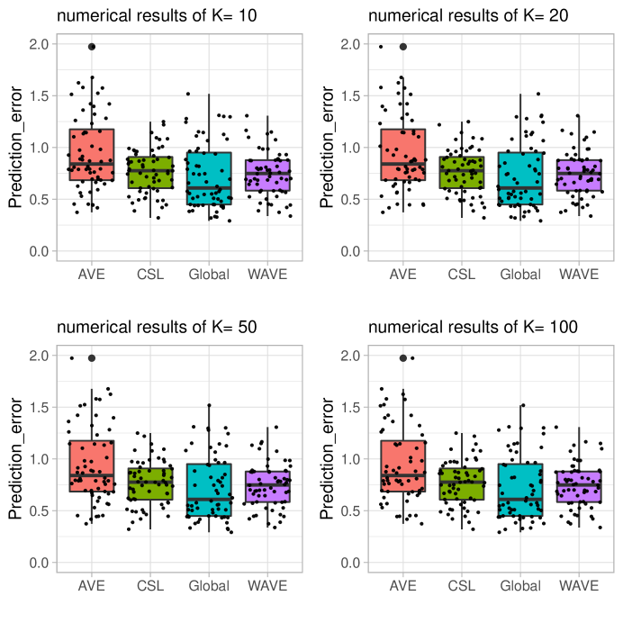
Figure 1: The prediction error in 60 days of different methods, where Global represents the case that the parameters are estimated by pooling the samples all together.

6.2 Application to Airline Data

The Airline Dataset records the flight information about U.S. airlines from 1988 to 2008. This dataset is distributed in 21 files, recording the flight information of 21 years. Totally, it has about 113 million records, each consists of a binary response variable for delayed status, and 11 covariates including departure time, scheduled departure time, scheduled arrival time, elapsed time, distance of the flight, flight date (Year, Month, Day of month and Day of week), carrier information, origin and destination. All numerical variables are standardized to have a mean of zero and a variance of one.

The task is to predict the delayed status of a flight given all other flight information. Thus, we build a logistic model to link the response to the covariates. To capture possible seasonal patterns, we convert the time variables Month and DayofWeek to dummies. We also convert the Carrier, Destination and Origin to dummies. See Table 5 for the details of dummy transformation. After above variable argument procedure, a total of 185 variables are involved in the model, and the overall size of the dataset is over 100 GB, which can hardly be loaded into the memory in a single computer. Thus, it is reasonable to take the distributed way to deal with this dataset. We use the data in first 20 files (flight records from 1988 to 2007) to train the logistic model and the data in 2008 as the validation set. In each file, the training of logistic model involves the selection of tuning parameter, to save the running time, we determine it with 2-fold cross-validation method by splitting the data in each file into two parts with a $7:3$ ratio as training set and testing set, respectively.

Table 6 reports the testing error of different methods, from which it can be observed that the newly proposed WAVE achieves the minimal misclassification rate, while the two competitors, CSL and AVE have an unsatisfactory performance. Moreover, the first 8 largest and smallest estimated coefficients by WAVE are also displayed in Table 7. From this table, we can conclude that the variable actElapsedTime and distance have very obvious effects on predictiong the delay status of a flight. Specifically, a longer actual elapsed time and a shorter distance are intended to delay a flight. Secondly, different origins and destinations do have positive or negative effect on the delay of a flight.

Table 5: Variable description for the U.S. airline data. Non-categorical numerical variables are standardized to have mean zero and variance one.

Variable	Description	Variable used in the model
Delayed	1 for Delay; 0 for Not-delay.	Used as the response variable
DepTime	Actual departure time	Used as numerical variable (in hours)
CRSDepTime	Scheduled departure time	Used as numerical variable (in hours)
CRSArrTime	Scheduled arrival time	Used as numerical variable (in hours)
ElapsedTime	Actual elapsed time	Used as numerical variable (in hours)
Distance	Distance between the origin and destination	Used as numerical variable (in 1000 miles)
DayofMonth	Which day of the month	Used as numerical variable
Month	Which month of the year	Converted to 11 dummies
DayofWeek	Which day of the week	Converted to 6 dummies
Carrier	Flight carrier code for 29 carriers	Top 12 carries converted to 12 dummies
Destination	Destination of the flight	Top 75 cities converted to 75 dummies
Origin	Departing origin	Top 75 cities converted to 75 dummies

Table 6: Misclassification rate for the data in 2008 of different methods.

Method	WAVE	CSL	AVE
Testing error	0.2874	0.3270	0.3938

Table 7: The largest and smallest top 8 estimated coefficients by WAVE and corresponding variables. Ori represents the departing origin and Des represents the destination of a flight.

Variable Name	Estimated Coef	Variable Name	Estimated Coef
actElapsedTime	7.3569	distance	-14.4254
HNL(Ori)	2.8456	JFK(Oir)	-2.7971
SJU(Des)	1.9142	LGA(Ori)	-2.6508
ANC(Ori)	1.6218	EWR(Ori)	-2.5201
SMF(Ori)	1.3852	BOS(Ori)	-2.4231
PDX(Ori)	1.3171	SNA(Des)	-1.9887
ONT(Ori)	1.2179	PVD(Ori)	-1.8861
RNO(Ori)	1.2177	SFO(Des)	-1.8590

7 Conclusions

This paper proposes a new distributed estimator named weighted average estimate (WAVE for short) in the context of high-dimensional regressions. The notable feature of WAVE is that it achieves a balance between the communication efficient and statistical efficient. On the one hand, WAVE consumes very low communication cost because each worker is required to deliver only two vectors to the master. On the other hand, WAVE is more statistical efficient since the estimate in workers with a larger variance would be allocated to a smaller weight. It is shown that WAVE is effective even when the samples across local machines have different mean and covariance. Moreover, WAVE can be applied to a wide range of scenarios, including the linear model under the huber loss and the generalized linear model. Actually, WAVE can be extended to more general models like semi-parametric models, quantile regression models and etc., in which the parameter of interest can be aggregated via the formula like (8). The difference lies at that the diagonal matrix ${\bf\Lambda}$ should be customized according to specific model, relevant research can be explored in future study.

Acknowledgments

We would like to acknowledge support for these projects from Key NSF of China under Grant No. 62136005, the NSF of China under Grant No. 61922087, 12001486.

Appendix

In this appendix, we prove the Theorem 1 and 2.

Proof of Theorem 1. The proof of this theorem is similar to that of Theorem 4 in Zou (2006), here we only give an outline.

We first prove the result (2). For the notational simplicity, we assume a simple situation that there is only one worker and the total sample size is $n$. Let $\bm{\beta}=\bm{\beta}^{*}+\frac{\bm{u}}{\sqrt{n}}$, define

$$\Gamma_{n}(\bm{u})=\sum_{i=1}^{n}\mathcal{L}(Y_{i},\bm{X}_{i}^{\top}(\bm{\beta}^{*}+{\bm{u}}/{\sqrt{n}}))+\lambda_{n}\sum_{j=1}^{p}\hat{\omega}_{j}|\beta_{j}^{*}+u_{j}/\sqrt{n}|.$$

By Taylor expansion, it has that $\bm{\Gamma}_{n}(\bm{u})-\bm{\Gamma}_{n}(\bm{0})=\bm{H}_{n}(\bm{u})=A_{n1}(\bm{u})+A_{n2}(\bm{u})+A_{n3}(\bm{u})+A_{n4}(\bm{u})$, where

$$A_{n1}(\bm{u}) = \sum_{i=1}^{n}\mathcal{L}^{\prime}(Y_{i},\bm{X}_{i}^{\top}\bm{\beta}^{*})\frac{\bm{X}_{i}^{\top}\bm{u}}{\sqrt{n}}$$

$$A_{n2}(\bm{u}) = \frac{1}{2}\sum_{i=1}^{n}\mathcal{L}^{\prime\prime}(Y_{i},\bm{X}_{i}^{\top}\bm{\beta}^{*})\frac{(\bm{X}_{i}^{\top}\bm{u})^{2}}{n}$$

$$A_{n3}(\bm{u}) = \frac{1}{6}\sum_{i=1}^{n}\mathcal{L}^{\prime\prime\prime}(Y_{i},\bm{X}_{i}^{\top}\widetilde{\bm{\beta}}^{*})\frac{(\bm{X}_{i}^{\top}\bm{u})^{3}}{n^{3/2}}$$

$$A_{n4}(\bm{u}) = \frac{\lambda_{n}}{\sqrt{n}}\sum_{j=1}^{p}\hat{\omega}_{j}\sqrt{n}\left(|\beta_{j}^{*}+\frac{u_{j}}{\sqrt{n}}|-|\beta_{j}^{*}|\right)$$

where $\widetilde{\bm{\beta}}^{*}$ is between $\bm{\beta}^{*}$ and $\bm{\beta}^{*}+\bm{u}/\sqrt{n}$. Next, we give the limit behavior of each term. For $A_{n1}(\bm{u})$, because $E(\mathcal{L}^{\prime}(Y_{i},\bm{X}_{i}^{\top}\bm{\beta}^{*}){\bm{X}_{i}^{\top}\bm{u}}/{\sqrt{n}})=0$, thus the central limit theorem tells us that $A_{n1}(\bm{u})\rightarrow\bm{u}^{\top}N(\bm{0},\bm{\Phi})$, where $\bm{\Phi}=E(\mathcal{L}^{\prime}(Y_{i},\bm{X}_{i}^{\top}\bm{\beta}^{*})^{2}\bm{X}_{i}\bm{X}_{i}^{\top})$. For the second term $A_{n2}(\bm{u})$, the law of large numbers says that

$$\frac{1}{n}\sum_{i=1}^{n}\mathcal{L}^{\prime\prime}(Y_{i},\bm{X}_{i}^{\top}\bm{\beta}^{*})\bm{X}_{i}\bm{X}_{i}^{\top}\rightarrow\bm{\Psi}=E(L^{\prime\prime}(Y_{i},\bm{X}_{i}^{\top}\bm{\beta}^{*})\bm{X}_{i}\bm{X}_{i}^{\top}).$$

Thus $A_{n2}(\bm{u})\rightarrow_{p}\frac{1}{2}\bm{u}^{\top}\bm{\Psi}\bm{u}$. For the third term $A_{n3}(\bm{u})$, by condition (C2), it can be bounded as

$$\sqrt{n}A_{n3}(\bm{u})\leq\frac{1}{n}\sum_{i=1}^{n}\mathcal{L}^{{}^{\prime\prime\prime}}(\bm{X}_{i})|\bm{X}_{i}^{\top}\bm{u}|^{3}\rightarrow_{p}E(L(\bm{X})|\bm{X}^{\top}\bm{u}|^{3})<\infty.$$

For the last term $A_{n4}$, if $\beta_{j}^{*}\neq 0$, then $\hat{\omega}_{j}\rightarrow_{p}|\beta_{j}^{*}|^{-\xi}$ and $\sqrt{n}(|\beta_{j}^{*}+\frac{u_{j}}{\sqrt{n}}|-|\beta_{j}^{*}|)\leq|u_{j}|$. By Slutsky’s theorem, $\frac{\lambda_{n}}{\sqrt{n}}\hat{\omega}_{j}\sqrt{n}(|\beta_{j}^{*}+\frac{u_{j}}{\sqrt{n}}|-|\beta_{j}^{*}|)\rightarrow_{p}0$. If $\beta_{j}^{*}=0$, then $\sqrt{n}(|\beta_{j}^{*}+\frac{u_{j}}{\sqrt{n}}|-|\beta_{j}^{*}|)=|u_{j}|$ and $\frac{\lambda_{n}}{\sqrt{n}}\hat{\omega}_{j}=\frac{\lambda_{n}}{\sqrt{n}}n^{\xi/2}(|\sqrt{n}\hat{\beta}_{j}|)^{-\xi}$, where $\sqrt{n}\hat{\beta}_{j}=O_{p}(1)$.

Consequently, by the Slutsky’s theorem, we have $\bm{H}_{n}(\bm{u})\rightarrow_{d}\bm{H}(\bm{u})$, where

$$\bm{H}(\bm{u})=\begin{cases}\frac{1}{2}\bm{u}_{\mathcal{A}}^{\top}\bm{\Psi}_{\mathcal{A}}\bm{u}_{\mathcal{A}}-\bm{u}_{\mathcal{A}}^{\top}\bm{W}_{\mathcal{A}}&\text{ if }u_{j}=0\mbox{~{}for~{}}\forall j\notin\mathcal{A}\\ \infty&\text{ otherwise }\end{cases}$$

where $\bm{W}\sim N(\bm{0},\bm{\Phi})$. As $\bm{H}_{n}$ is convex and the unique minimum of $\bm{H}$ is $(\bm{\Psi}^{-1}_{\mathcal{A}}\bm{W}_{\mathcal{A}},0)^{\top}$. Then we have

$$\hat{\bm{u}}_{\mathcal{A}}\rightarrow_{d}\bm{\Psi}^{-1}_{\mathcal{A}}\bm{W}_{\mathcal{A}}\mbox{~{}and~{}}\hat{\bm{u}}_{\mathcal{A}^{c}}\rightarrow_{d}\bm{0}.$$

The asymptotic normality is proven.

The selection consistency can be proved by the same spirit as that in Zou (2006), thus we omit the details. One can refer to this literature for a completed reading.

$\square$

Proof of Theorem 2. We first prove the result (2), then (1) and (3).

Proof of result (2). Let

$$Q_{\nu}(\bm{\beta})=\frac{1}{2}\bm{\beta}^{\top}\left(\sum_{j=1}^{K}\alpha_{j}\widehat{\bm{\Lambda}}_{j}\right)\bm{\beta}-\bm{\beta}^{\top}\sum_{j=1}^{K}\alpha_{j}\widehat{\bm{\Lambda}}_{j}\widehat{\bm{\beta}}_{j}+\nu\sum_{j=1}^{p}\hat{\gamma}_{j}|\beta_{j}|.$$

Obviously, $Q_{\nu}(\bm{\beta})$ is a strictly convex function, thus we can achieve a global minimizer, denoted as $\widetilde{\bm{\beta}}_{\nu}$. Let $\widetilde{\bm{\beta}}_{\nu}=\bm{\beta}^{*}+a_{N}\bm{u}$. If $a_{N}\sqrt{N}=O_{p}(1)$, the proof is trivial. Thus, we suppose $a_{N}\sqrt{N}\rightarrow\infty$, then it has that

$$N(Q_{\nu}(\bm{\beta}^{*}+a_{N}\bm{u})-Q_{\nu}(\bm{\beta}^{*}))$$

$$= \frac{1}{2}a_{N}^{2}N\bm{u}^{\top}\left(\sum_{j=1}^{K}\alpha_{j}\widehat{\bm{\Lambda}}_{j}\right)\bm{u}+a_{N}\sqrt{N}\bm{u}^{\top}\sum_{j=1}^{K}\alpha_{j}\widehat{\bm{\Lambda}}_{j}\sqrt{N}(\bm{\beta}^{*}-\widehat{\bm{\beta}}_{j})$$

$$+N\nu_{N}\sum_{j=1}^{p}\hat{\gamma}_{j}(|\beta_{j}^{*}+a_{N}u_{j}|-|\beta_{j}^{*}|)$$

$$\geq \frac{1}{2}a_{N}^{2}N\bm{u}^{\top}\left(\sum_{j=1}^{K}\alpha_{j}\widehat{\bm{\Lambda}}_{j}\right)\bm{u}+a_{N}\sqrt{N}\bm{u}^{\top}\sum_{j=1}^{K}\alpha_{j}\widehat{\bm{\Lambda}}_{j}\sqrt{N}(\bm{\beta}^{*}-\widehat{\bm{\beta}}_{j})$$ (13)

$$-a_{N}\sqrt{N}\nu_{N}\sqrt{N}\hat{\gamma}_{\max_{\mathcal{A}}}\sum_{j\in\mathcal{A}}u_{j},$$ (14)

where $\hat{\gamma}_{\max_{\mathcal{A}}}=\max_{j\in\mathcal{A}}\hat{\gamma}_{j}$, and the inequality holds because

$$\sum_{j=1}^{p}\hat{\gamma}_{j}(|\beta_{j}^{*}+N^{-1/2}u_{j}|-|\beta_{j}^{*}|)\geq\sum_{j\in\mathcal{A}}\hat{\gamma}_{j}(|\beta_{j}^{*}+N^{-1/2}u_{j}|-|\beta_{j}^{*}|)\geq-N^{-1/2}\nu_{N}\hat{\gamma}_{\max_{\mathcal{A}}}\sum_{j\in\mathcal{A}}u_{j}$$

since $u_{j}=0$ for $j\in\mathcal{A}$. Note that the term in (14) is $o_{p}(a_{N}\sqrt{N})$ under the condition $\nu_{N}\sqrt{N}\rightarrow 0$. For the second term, it is of order $O_{p}(a_{N}\sqrt{N})$ when $K/\sqrt{N}\rightarrow 0$. Thus, the first term in (13) dominates the behavior of (13) and (14) as $N$ goes to infinity. Consequently, with probability approaching to 1, it has that $Q_{\nu}(\widetilde{\bm{\beta}}_{\nu})\geq Q_{\nu}(\bm{\beta}^{*})$. This conclusion violates the fact $Q_{\nu}(\widetilde{\bm{\beta}}_{\nu})\leq Q_{\nu}(\bm{\beta}^{*})$. We then can conclude that $\widetilde{\bm{\beta}}_{\nu}-\bm{\beta}=O_{p}(1/\sqrt{N})$.

Proof of result (1). If is sufficient to verify that $P(\widetilde{\beta}_{\nu,j}=0)\rightarrow 1$ for $j\notin\mathcal{A}$. We prove this conclusion by contradiction. Suppose $\widetilde{\beta}_{\nu,j}\neq 0$ for $j\notin\mathcal{A}$, then the derivative of $Q_{\nu}(\bm{\beta})$ w.r.t $\beta_{j}$ is

$$\frac{\partial Q_{\nu}(\bm{\beta})}{\partial\beta_{j}}\bigg{|}_{\beta_{j}=\tilde{\beta}_{\nu,j}}=\sum_{k=1}^{K}\alpha_{k}(\widehat{\bm{\Lambda}}_{k})_{jj}(\tilde{\beta}_{\nu,j}-\hat{\beta}_{j})+\nu\hat{\gamma}_{j}|\tilde{\beta}_{\nu,j}|$$

where $(\widehat{\bm{\Lambda}}_{k})_{jj}$ is the $j$-th diagonal element of $\widehat{\bm{\Lambda}}_{k}$. It is easy to prove that $\sqrt{N}(\tilde{\beta}_{\nu,j}-\hat{\beta}_{j})=O_{p}(1)$. Thus, under the condition $\nu\sqrt{N}\hat{\gamma}_{j}\rightarrow\infty$ for $j\notin\mathcal{A}$, we have $\sqrt{N}\frac{\partial Q_{\nu}(\bm{\beta})}{\partial\beta_{j}}\bigg{|}_{\beta_{j}=\tilde{\beta}_{\nu,j}}\rightarrow\infty$, which is violated the fact $\frac{\partial Q_{\nu}(\bm{\beta})}{\partial\beta_{j}}\bigg{|}_{\beta_{j}=\tilde{\beta}_{\nu,j}}=O_{p}(1/\sqrt{N})$

Proof of result (3). Let $\mathcal{L}^{\prime}_{\bm{\beta}}(Y_{i},\bm{X}_{i}^{\top}\bm{\beta})$ be the partial derivative of $\mathcal{L}(Y_{i},\bm{X}_{i}^{\top}\bm{\beta})$ with respect to $\bm{\beta}$, and for the convenience, let $\mathcal{L}_{\bm{\beta},k}^{\prime}(\bm{\beta}_{\mathcal{A}})=\frac{1}{n_{k}}\sum_{i\in\mathcal{I}_{k}}\mathcal{L}_{\bm{\beta}}(Y_{i},\bm{X}_{\mathcal{A},i}^{\top}\bm{\beta}_{\mathcal{A}})$. We define $\mathcal{L}^{\prime\prime}_{\bm{\beta},k}$ and $\mathcal{L}^{\prime\prime}_{\bm{\beta},k}$ with a similar way. Let $\widehat{\bm{\beta}}_{\mathcal{A},k}$ be the adaptive lasso estimator in $k$-th worker. By the Taylor expansion, it has that

$$\bm{0}=\mathcal{L}_{\bm{\beta},k}^{\prime}(\widehat{\bm{\beta}}_{\mathcal{A},k})=\mathcal{L}_{\bm{\beta},k}^{\prime}({\bm{\beta}}^{*}_{\mathcal{A}})+\mathcal{L}^{\prime\prime}_{\bm{\beta},k}(\bm{\beta}^{*})(\widehat{\bm{\beta}}_{\mathcal{A},k}-\bm{\beta}^{*}_{\mathcal{A}})+(\bm{\beta}_{\mathcal{A}}^{0}-\bm{\beta}_{\mathcal{A}}^{*})^{\top}\mathcal{L}^{\prime\prime\prime}_{\bm{\beta},k}(\bm{\beta}^{0}_{\mathcal{A}})(\bm{\beta}^{0}_{\mathcal{A}}-\bm{\beta}_{\mathcal{A}}^{*})$$

where $\bm{\beta}^{0}_{\mathcal{A}}$ is between $\widehat{\bm{\beta}}_{\mathcal{A},k}$ and $\bm{\beta}^{*}_{\mathcal{A}}$. Since $\widehat{\bm{\beta}}_{\mathcal{A},k}-\bm{\beta}^{*}_{\mathcal{A}}=O_{p}(1/\sqrt{n_{k}})$, and $\mathcal{L}^{\prime\prime}_{\bm{\beta},k}=\bm{\Psi}_{\mathcal{A},k}+O_{p}(1/\sqrt{n_{k}})$, thus the last term in above formula is $o_{p}(1/\sqrt{n_{k}})$, we have

$$\widehat{\bm{\beta}}_{\mathcal{A},k}-\bm{\beta}^{*}_{\mathcal{A}}=\bm{\Psi}_{\mathcal{A},k}^{-1}\mathcal{L}_{\bm{\beta},k}^{\prime}({\bm{\beta}}^{*}_{\mathcal{A}})+O_{p}(1/n_{k}),$$

On the other hand, it can be proved that

$$\widehat{\bm{\Lambda}}_{\mathcal{A},k}=\mbox{diag}(\widehat{\bm{\Sigma}}^{-1}_{\mathcal{A},k})=\bm{\Lambda}_{\mathcal{A},k}=\mbox{diag}\left(\bm{\Psi}_{\mathcal{A},k}\bm{\Phi}^{-1}_{\mathcal{A},k}\bm{\Psi}_{\mathcal{A},k}\right)+O_{p}(1/\sqrt{n_{k}})$$

Since $\mathcal{L}_{\bm{\beta},k}^{\prime}({\bm{\beta}}_{\mathcal{A}}^{*})=O_{p}(1/\sqrt{n_{k}})$, we have that

$$\sum_{j=1}^{K}\alpha_{j}\widehat{\bm{\Lambda}}_{\mathcal{A},j}(\widehat{\bm{\beta}}_{\mathcal{A},j}-\bm{\beta}^{*}_{\mathcal{A}})=\sum_{j=1}^{K}\alpha_{j}\bm{\Lambda}_{\mathcal{A},j}\bm{\Psi}^{-1}_{\mathcal{A},j}\mathcal{L}^{\prime}_{\bm{\beta},j}(\bm{\beta}^{*}_{\mathcal{A}})+O_{p}\left(\sum_{j=1}^{K}\frac{1}{n_{k}}\right).$$ (15)

Consequently, it has that

$$\widetilde{\bm{\beta}}_{\mathcal{A}}-\bm{\beta}^{*}_{\mathcal{A}} = \left(\sum_{j=1}^{K}\alpha_{j}\bm{\Lambda}_{\mathcal{A},j}\right)^{-1}\left\{\sum_{j=1}^{K}\alpha_{j}\bm{\Lambda}_{\mathcal{A},j}\bm{\Psi}^{-1}_{\mathcal{A},j}\mathcal{L}^{\prime}_{\bm{\beta},j}(\bm{\beta}^{*}_{\mathcal{A}})+O_{p}\left(\sum_{j=1}^{K}\frac{1}{n_{k}}\right)\right\}$$

$$= \left(\sum_{j=1}^{K}\alpha_{j}\bm{\Lambda}_{\mathcal{A},j}\right)^{-1}\frac{1}{N}\sum_{j=1}^{K}\sum_{i\in\mathcal{I}_{j}}\bm{\Lambda}_{\mathcal{A},j}\bm{\Psi}^{-1}_{\mathcal{A},j}\mathcal{L}_{\bm{\beta}}(Y_{i},\bm{X}_{\mathcal{A},i}^{\top}\bm{\beta}^{*}_{\mathcal{A}})+O_{p}\left(\sum_{j=1}^{K}\frac{1}{n_{k}}\right).$$

Since $E\bm{\Lambda}_{\mathcal{A},j}\bm{\Psi}^{-1}_{\mathcal{A},j}\mathcal{L}_{\bm{\beta}}(Y_{i},\bm{X}_{\mathcal{A},i}^{\top}\bm{\beta}^{*}_{\mathcal{A}})=\bm{0}$ and

$$\mbox{Var}_{i\in\mathcal{I}_{j}}(\bm{\Lambda}_{\mathcal{A},j}\bm{\Psi}^{-1}_{\mathcal{A},j}\mathcal{L}_{\bm{\beta}}(Y_{i},\bm{X}_{\mathcal{A},i}^{\top}\bm{\beta}^{*}_{\mathcal{A}}))=\bm{\Omega}_{\mathcal{A},j}=\bm{\Lambda}_{\mathcal{A},j}\bm{\Psi}^{-1}_{\mathcal{A},j}\bm{\Phi}_{\mathcal{A},j}\bm{\Psi}^{-1}_{\mathcal{A},j}\bm{\Lambda}_{\mathcal{A},j}.$$

Thus, under condition (C1) and (C2) and Lemma 3, it has that

$$\frac{1}{N}\sum_{j=1}^{K}\sum_{i\in\mathcal{I}_{j}}\bm{\Lambda}_{\mathcal{A},j}\bm{\Psi}^{-1}_{\mathcal{A},j}\mathcal{L}_{\bm{\beta}}(Y_{i},\bm{X}_{\mathcal{A},i}^{\top}\bm{\beta}^{*}_{\mathcal{A}})\sim N(\bm{0},\frac{1}{N}\bm{S}_{N})$$ (16)

where $\bm{S}_{N}=\frac{1}{N}\sum_{j=1}^{K}\sum_{i\in\mathcal{I}_{j}}\bm{\Omega}_{\mathcal{A},j}=\sum_{j=1}^{K}\alpha_{j}\bm{\Omega}_{\mathcal{A},j}$. Finally, we get the conclusion that

$$\widetilde{\bm{\beta}}_{\mathcal{A}}-\bm{\beta}^{*}_{\mathcal{A}}\sim N(\bm{0},\frac{1}{N}\bm{V}_{N}^{-1}\bm{S}_{N}\bm{V}_{N}^{-1}),$$ (17)

where $\bm{V}_{N}=\sum_{j=1}^{K}\alpha_{j}\bm{\Lambda}_{\mathcal{A},j}$.

$\square$

Lemma 3

(The multivariate Lyapunov CLT). Let $\bm{X}_{i},i=1,\cdots,n$ be $n$ independent but not necessary identical distributed random vector with mean $\bm{\mu}_{i}$ and covariance $\bm{\Sigma}_{i}$, then it has that

$$\frac{1}{n}\sum_{i=1}^{n}\bm{X}_{i}\sim N(\bm{v}_{n},\bm{C}_{n}),$$ (18)

where $\bm{v}_{n}=\frac{1}{n}\sum_{i=1}^{n}\bm{\mu}_{i}$ and $\bm{C}_{n}=\frac{1}{n^{2}}\sum_{i=1}^{n}\bm{\Sigma}_{i}$.

Proof. Let $\boldsymbol{Z}_{n}=\frac{1}{n}\sum_{i=1}^{n}\boldsymbol{X}_{i}$ and $\boldsymbol{Z}_{n}=(Z_{n1},\cdots,Z_{np})^{\top}$, $Y_{n}=\boldsymbol{a}^{\top}\boldsymbol{Z}_{n}=\frac{1}{n}\sum_{i=1}^{n}\boldsymbol{a}^{\top}\boldsymbol{X}_{i}$. Because $\boldsymbol{a}^{\top}\boldsymbol{X}_{i}$ are independent with mean $\boldsymbol{a}^{\top}\boldsymbol{\mu}_{i}$ and covariance $\boldsymbol{a}^{\top}\boldsymbol{\Sigma}_{i}\boldsymbol{a}$, thus by the univariate Lyapounov CLT(provide that the condition holds), then it can be proved that

$$\frac{1}{n}\sum_{i=1}^{n}(\boldsymbol{a}^{\top}\boldsymbol{X}_{i}-\boldsymbol{a}^{\top}\boldsymbol{\mu}_{i})\sim N(0,\frac{1}{n^{2}}s_{n}^{2})$$

where $s_{n}^{2}=\sum_{i=1}^{n}\boldsymbol{a}^{\top}\boldsymbol{\Sigma}_{i}\boldsymbol{a}$, namely, $Y_{n}\sim N(\gamma_{n},\frac{1}{n^{2}}s_{n}^{2})$, where $\gamma_{n}=\frac{1}{n}\sum_{i=1}^{n}\boldsymbol{a}^{\top}\boldsymbol{\mu}_{i}$. So, the c.h.f of $Y_{n}$ is

$$\phi_{Y_{n}}(t)=E\exp(itY_{n})=E\exp(it\boldsymbol{a}^{\top}\boldsymbol{Z}_{n})=E\exp(it\gamma_{n}-\frac{1}{2n^{2}}t^{2}s_{n}^{2})$$

$$= E\exp(it\frac{1}{n}\sum_{i=1}^{n}\boldsymbol{a}^{\top}\boldsymbol{\mu}_{i}-\frac{1}{2n^{2}}t^{2}\sum_{i=1}^{n}\boldsymbol{a}^{\top}\boldsymbol{\Sigma}_{i}\boldsymbol{a})=E\exp(i\boldsymbol{a}^{\top}\boldsymbol{v}_{n}-\frac{1}{2}\boldsymbol{a}^{\top}\boldsymbol{C}_{n}\boldsymbol{a})=\phi_{\boldsymbol{Z}_{n}}(\boldsymbol{a})$$

where the last equality holds by setting $t=1$, $\boldsymbol{v}_{n}=\frac{1}{n}\sum_{i=1}^{n}\boldsymbol{\mu}_{i}$, $\boldsymbol{C}_{n}=\frac{1}{n^{2}}\sum_{i=1}^{n}\boldsymbol{\Sigma}_{i}$, namely, $\boldsymbol{Z}_{n}$ follows the norma distribution with mean $\boldsymbol{v}_{n}$ and covariance $\boldsymbol{C}_{n}$.

The remaining problem is to prove the Lyapunov’s condition that there exists a $\delta>0$ such that

$$\lim_{n\rightarrow\infty}\frac{1}{s_{n}^{2+\delta}}\sum_{i=1}^{n}E(|\boldsymbol{a}^{\top}\boldsymbol{X}_{i}-\boldsymbol{a}^{\top}\boldsymbol{\mu}_{i}|^{2+\delta})=0$$

Suppose the following two conditions hold:

(A1)

There are two constants $c$ and $C$ such that

$$c\leq\lambda_{\min}(E\bm{X}_{i}\bm{X}_{i}^{\top})\leq\lambda_{\max}(E\bm{X}_{i}\bm{X}_{i}^{\top})\leq C,\mbox{~{}for~{}all~{}}i,$$

where $\lambda_{\min/\max}(\bm{A})$ is the minimal/maximal eigenvalue of matrix $\bm{A}$.

(A2)

There exists a constant $M$ such that for any $k=1,2,\cdots,p$, it has that

$$EX_{ik}^{4}<M.$$

We consider the case $\delta=2$. Without loss of generality, we assume $\bm{\mu}_{i}=\bm{0}$. Firstly, it has that

$$\sum_{i=1}^{n}E(|\boldsymbol{a}^{\top}\boldsymbol{X}_{i}|^{2+\delta})=\sum_{i=1}^{n}E(|\boldsymbol{a}^{\top}\boldsymbol{X}_{i}|^{4})=\sum_{i=1}^{n}\left\{E\left(\sum_{j=1}^{p}a_{j}X_{ij}\right)^{4}\right\}$$

$$= \sum_{i=1}^{n}\left\{E\left(\sum_{k,l=1}^{p}a_{k}a_{l}X_{ik}X_{il}\right)^{2}\right\}\leq\sum_{i=1}^{n}\left\{E\left(\sum_{k,l=1}^{p}\frac{a_{k}^{2}X_{ik}^{2}+a_{l}^{2}X_{il}^{2}}{2}\right)^{2}\right\}$$

$$= \sum_{i=1}^{n}\left\{E\left(p\sum_{k=1}^{p}a_{k}^{2}X_{ik}^{2}\right)^{2}\right\}=\sum_{i=1}^{n}\left\{p^{2}E\left(\sum_{k,l=1}^{p}a_{k}^{2}a_{l}^{2}X_{ik}^{2}X_{il}^{2}\right)\right\}$$

$$\leq \sum_{i=1}^{n}\left(p^{2}M\sum_{k,l=1}^{p}a_{k}^{2}a_{l}^{2}\right)=\sum_{i=1}^{n}p^{2}M\left(\bm{a}^{\top}\bm{a}\right)^{2}=np^{2}M(\bm{a}^{\top}\bm{a})^{2}$$

where the first inequality holds because of the fact that $\frac{a^{2}+b^{2}}{2}\geq|ab|\geq ab$, and the second inequality holds because of condition (C2). Now, as $n\rightarrow\infty$, we have

$$\frac{1}{s_{n}^{2+\delta}}\sum_{i=1}^{n}E(|\boldsymbol{a}^{\top}\boldsymbol{X}_{i}|^{2+\delta})=\frac{\sum_{i=1}^{n}E(|\boldsymbol{a}^{\top}\boldsymbol{X}_{i}|^{4})}{\left(\sum_{i=1}^{n}\boldsymbol{a}^{\top}\boldsymbol{E}(\bm{X}_{i}\bm{X}_{i}^{\top})\boldsymbol{a}\right)^{2}}\leq\frac{np^{2}M(\bm{a}^{\top}\bm{a})^{2}}{(nc\bm{a}^{\top}\bm{a})^{2}}=\frac{p^{2}M}{nc^{2}}\rightarrow 0$$

if $p=o(\sqrt{n})$, where the inequality holds because condition (C1).

$\square$

References

- Battey et al. (2018) Battey, H., Fan, J., Liu, H., Lu, J. and Zhu, Z., 2018. Distributed testing and estimation under sparse high dimensional models. Annals of statistics, 46, 1352–1382.
- Chang et al. (2017) Chang, X., Lin, S.B. and Wang, Y., 2017. Divide and conquer local average regression. Electronic Journal of Statistics, 11, 1326-1350.
- Chang et al. (2017) Chang, X., Lin, S.B. and Zhou, D.X., 2017. Distributed semi-supervised learning with kernel ridge regression. Journal of Machine Learning Research, 18, 1493-1514.
- Chen and Peng (2021) Chen, S.X. and Peng, L., 2021. Distributed statistical inference for massive data. Annals of Statistics, 49, 2851-2869.
- Chen et al. (2019) Chen, X., Liu, W. and Zhang, Y., 2019. Quantile regression under memory constraint. Annals of Statistics, 47, 3244-3273.
- Chen et al. (2021) Chen, X., Cheng, J.Q. and Xie, M.G., 2021. Divide-and-conquer methods for big data analysis. arXiv preprint:2102.10771.
- Chen and Xie (2014) Chen, X. and Xie, M.G., 2014. A split-and-conquer approach for analysis of extraordinarily large data. Statistica Sinica, 24, 1655-1684.
- Fan et al. (2017) Fan, J., Li, Q. and Wang, Y., 2017. Estimation of high dimensional mean regression in the absence of symmetry and light tail assumptions. Journal of the Royal Statistical Society: Series B (Statistical Methodology), 79, 247-265.
- Fan et al. (2001) Fan, J. and Li. R., 2001. Variable selection via nonconcave penalized likelihood and its oracle properties. Journal of the American Statistical Association, 96, 1348–1360.
- Fan et al. (2019) Fan, J., Wang, D., Wang, K. and Zhu, Z., 2019. Distributed estimation of principal eigenspaces. Annals of statistics, 47, 3009-3031.
- Gao et al. (2021) Gao, Y., Liu, W., Wang, H., Wang, X., Yan, Y. and Zhang, R., 2021. A review of distributed statistical inference. Statistical Theory and Related Fields, DOI: 10.1080/24754269.2021.1974158.
- Huang and Huo (2019) Huang, C. and Huo, X., 2019. A distributed one-step estimator. Mathematical Programming, 174, 41-76.
- Huang et al. (2022) Huang, B., Liu, Y. and Peng, L., 2022. Distributed inference for two-sample U-statistics in massive data analysis. Statistica Sinica, online published.
- Huber (1981) Huber P.J., 1981. Robust Statistics. Wiley.
- Jordan et al. (2019) Jordan, M.I., Lee, J.D. and Yang, Y., 2019. Communication-efficient distributed statistical inference. Journal of the American Statistical Association, 114, 668–681.
- Lee et al. (2017) Lee, J.D., Liu, Q., Sun, Y. and Taylor, J.E., 2017. Communication-efficient sparse regression. Journal of Machine Learning Research, 18, 115-144.
- Li et al. (2020) Li, X., Li, R., Xia, Z. and Xu, C., 2020. Distributed feature screening via componentwise debiasing. Journal of machine learning research, 21.
- Lin and Xi (2011) Lin, N. and Xi, R., 2011. Aggregated estimating equation estimation. Statistics and its Interface, 4, 73-83.
- Lv and Lian (2022) Lv, S. and Lian, H., 2022. Debiased Distributed Learning for Sparse Partial Linear Models in High Dimensions. Journal of Machine Learning Research, 23, 1-32.
- Tan et al. (2022) Tan, K., Battey, H. and Zhou, W., 2022. Communication-Constrained Distributed Quantile Regression with Optimal Statistical Guarantees. Journal of Machine Learning Research, 23, 1-61.
- Sun et al. (2020) Sun, Q., Zhou, W.X. and Fan, J., 2020. Adaptive huber regression. Journal of the American Statistical Association, 115, 254-265.
- Tang et al. (2020) Tang, L., Zhou, L. and Song, P.X.K., 2020. Distributed simultaneous inference in generalized linear models via confidence distribution. Journal of multivariate analysis, 176, DOI:10.1016/j.jmva.2019.104567.
- Tu et al. (2021) Tu, J., Liu, W. and Mao, X., 2021. Byzantine-robust distributed sparse learning for M-estimation. Machine Learning,
- Wang and Leng. (2007) Wang, H. and Leng. C., 2007. Unified Lasso estimation by least squares approximation. Journal of the American Statistical Association, 102, 1039-1048.
- Wang et al. (2021) Wang, F., Zhu Y., Huang, D., Qi, H., and Wang H., 2021. Distributed one-step upgraded estimation for non-uniformly and non-randomly distributed data. Computational Statistics and Data Analysis, 162, DOI:10.1016/j.csda.2021.107265
- Zhao et al. (2016) Zhao, T., Cheng, G. and Liu, H., 2016. A partially linear framework for massive heterogeneous data. Annals of statistics, 44, 1400-1437.
- Zhu et al. (2021) Zhu, X., Li, F. and Wang, H., 2021. Least-Square Approximation for a Distributed System. Journal of Computational and Graphical Statistics.
- Zou (2006) Zou, H., 2006. The adaptive lasso and its oracle properties. Journal of the American Statistical Association, 101, 1418-1429.