SPD domain-specific batch normalization to crack interpretable unsupervised domain adaptation in EEG

Abstract

Electroencephalography (EEG) provides access to neuronal dynamics non-invasively with millisecond resolution, rendering it a viable method in neuroscience and healthcare. However, its utility is limited as current EEG technology does not generalize well across domains (i.e., sessions and subjects) without expensive supervised re-calibration. Contemporary methods cast this transfer learning (TL) problem as a multi-source/-target unsupervised domain adaptation (UDA) problem and address it with deep learning or shallow, Riemannian geometry aware alignment methods. Both directions have, so far, failed to consistently close the performance gap to state-of-the-art domain-specific methods based on tangent space mapping (TSM) on the symmetric, positive definite (SPD) manifold. Here, we propose a machine learning framework that enables, for the first time, learning domain-invariant TSM models in an end-to-end fashion. To achieve this, we propose a new building block for geometric deep learning, which we denote SPD domain-specific momentum batch normalization (SPDDSMBN). A SPDDSMBN layer can transform domain-specific SPD inputs into domain-invariant SPD outputs, and can be readily applied to multi-source/-target and online UDA scenarios. In extensive experiments with 6 diverse EEG brain-computer interface (BCI) datasets, we obtain state-of-the-art performance in inter-session and -subject TL with a simple, intrinsically interpretable network architecture, which we denote TSMNet. Code: https://github.com/rkobler/TSMNet

1 Introduction

Electroencephalography (EEG) measures multi-channel electric brain activity from the human scalp with millisecond precision [1]. Transient modulations in the rhythmic brain activity can reveal cognitive processes [2], affective states [3] and a person’s health status [4]. Unfortunately, these modulations exhibit low signal-to-noise ratio (SNR), domain shifts (i.e., changes in the data distribution) and have low specificity, rendering statistical learning a challenging task - particularly in the context of brain-computer interfaces (BCI) [5] where the goal is to predict a target from a short segment of multi-channel EEG data in real-time.

Under domain shifts, domain adaptation (DA), defined as learning a model from a source domain that performs well on a related target domain, offers principled statistical learning approaches with theoretical guarantees [6, 7]. DA in the BCI field mainly distinguishes inter-session and -subject transfer learning (TL) [8]. In inter-session TL, domain shifts, are expected across sessions mainly due to mental drifts (low specificity) as well as differences in the relative positioning of the electrodes and their impedances. Inter-subject TL is more difficult, as domain shifts are additionally driven by structural and functional differences in brain networks as well as variations in the performed task [9].

These domain shifts are traditionally circumvented by recording labeled calibration data and fitting domain-specific models [10, 11]. As recording calibration data is costly, models that are robust to scarce data with low SNR perform well in practice. Currently, tangent space mapping (TSM) models [12, 13] operating with symmetric, positive definite (SPD) covariance descriptors of preprocessed data are considered state-of-the-art (SoA) [10, 14, 15]. They are well suited for EEG data as they exhibit invariances to linear mixing of latent sources [16], and are consistent [13] and intrinsically interpretable [17] estimators for generative models that encode label information with a log-linear relationship in source power modulations.

Competitive, supervised calibration-free methods are one of the long-lasting grand challenges in EEG neurotechnology research [5, 10, 18, 19, 15]. Among the applied transfer learning techniques, including multi-task learning [20] and domain-invariant learning [21, 22, 23], unsupervised domain adaptation (UDA) [24] is considered as key to overcome this challenge [10, 19]. Contemporary methods cast the problem as a multi source and target UDA problem and address it with deep learning [25, 26, 27, 28] or shallow, Riemannian geometry aware alignment methods [29, 30, 31, 32]. Successful methods must cope with notoriously small and heterogeneous datasets (i.e., dozens of domains with a few dozens observations per domain and class). In a recent, relatively large scale inter-subject and -dataset TL competition with few labeled examples per target domain [19], deep learning approaches that aligned the first and second order statistics either in input [33, 27] or latent space [34] obtained the highest scores. Whereas, in a pure UDA competition [15] with a smaller dataset, Riemannian geometry aware approaches dominated. With the increasing popularity of geometric deep learning [35], Ju and Guan [36] proposed an architecture based on SPD neural networks [37] to align SPD features in latent space and attained SoA scores. Despite the tremendous advances in recent years, the field still lacks methods that can consistently close the performance gap to state-of-the-art domain-specific methods.

To close this gap, we propose a machine learning framework around domain-specific batch normalization on the SPD manifold (Figure 1). The proposed framework is used to implement domain-specific TSM (Figure 1a), which requires tracking the domains’ Fréchet means in latent space as they are changing during training a typical TSM model in an end-to-end fashion (Figure 1b). After reviewing some preliminaries in section 2, we extend momentum batch normalization (MBN) [32] to SPDMBN that controls the Fréchet mean and variance of SPD data in section 3. In a theoretical analysis, we show under reasonable assumptions that SPDMBN can track and converge to the data’s true Fréchet mean, enabling, for the first time, end-to-end learning of feature extractors, TSM and tangent space classifiers. Building upon this insight, we combine SPDMBN with domain-specific batch normalization (DSBN) [38] to form SPDDSMBN (Figure 1a). A SPDDSMBN layer can transform domain-specific SPD inputs into domain-invariant SPD outputs (Figure 1c). Like DSBN, SPDDSMBN easily extends to multi-source, multi-target and online UDA scenarios. In section 4, we briefly review the generative model of EEG, before the proposed methods are combined in a simple, intrinsically interpretable network architecture, denoted TSMNet (Figure 1b). We obtain state-of-the-art performance in inter-session and -subject UDA on small and large scale EEG BCI datasets, and show in an ablation study that the performance increase is primarily driven by performing DSBN on the SPD manifold.

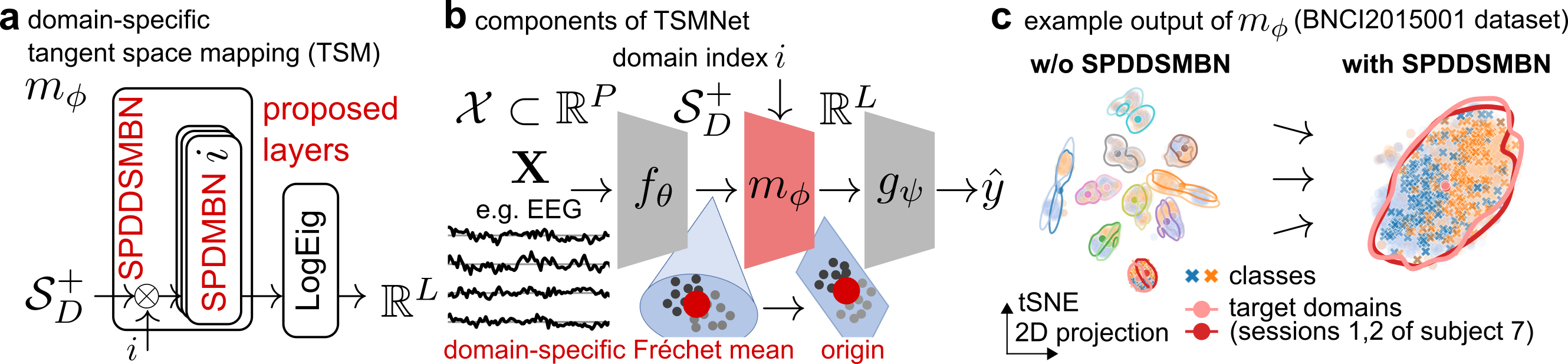
Figure 1: Visualization of the proposed framework around (a) SPD domain-specific momentum batch normalization (SPDDSMBN) that (b) learns parameters $\Theta=\{\theta,\phi,\psi\}$ of typical tangent space mapping (TSM) models end-to-end to crack multi-source/-target unsupervised domain adaptation on $\mathcal{S}^{+}_{D}$ for EEG data (c, illustrative example). For EEG data, we propose a simple, intrinsically interpretable parametrization of $f$ and $g$, denoted TSMNet, and obtain SoA performance.

2 Preliminaries

Multi-source multi-target unsupervised domain adaptation

Let $\mathcal{X}$ denote the space of input features, $\mathcal{Y}$ a label space, and $\mathcal{I}_{d}\subset\mathbb{N}$ an index set that contains unique domain identifiers. In the multi-source, multi-target unsupervised domain adaptation scenario considered here, we are given a set $\mathcal{T}^{source}=\{\mathcal{T}_{i}|i\in\mathcal{I}_{d}^{source}\subset\mathcal{I}_{d}\}$ with $|\mathcal{I}_{d}^{source}|=N$ domains. Each domain $\mathcal{T}_{i}=\{(\mathbf{X}_{ij},y_{ij})\}_{j=1}^{M}\sim P_{XY}^{i}$ contains $M$ observations of feature ($\mathbf{X}\in\mathcal{X}$) and label ($y\in\mathcal{Y}$) tuples sampled from a joint distribution $P_{XY}^{i}$. While the joint distributions can be different (but related) across domains, we assume that the class priors are the same (i.e., $P_{Y}^{i}=P_{Y}$). The goal is to learn a predictive function $h:\mathcal{X}\times\mathcal{I}_{d}\rightarrow\mathcal{Y}$ that, once fitted to $\mathcal{T}^{source}$, can generalize to unseen target domains $\mathcal{T}^{target}=\{\mathcal{T}_{l}|l\in\mathcal{I}_{d}^{target}\subset\mathcal{I}_{d},\mathcal{I}_{d}^{target}\cap\mathcal{I}_{d}^{source}=\emptyset\}$ merely based on unsupervised adaptation of $h$ to each target domain $\mathcal{T}_{l}$ once its label $l$ and features $\{\mathbf{X}_{lj}\}_{j=1}^{M}\sim P_{X}^{l}$ are revealed.

Riemannian geometry on $\mathcal{S}^{+}_{D}$

We start with recalling notions of geometry on the space of real $D\times D$ symmetric positive definite (SPD) matrices $\mathcal{S}^{+}_{D}=\{\mathbf{Z}\in\mathbb{R}^{D\times D}:\mathbf{Z}^{T}=\mathbf{Z},\mathbf{Z}\succ 0\}$. The space $\mathcal{S}^{+}_{D}$ forms a cone shaped Riemannian manifold in $\mathbb{R}^{D\times D}$ [39]. A Riemannian manifold $\mathcal{M}$ is a smooth manifold equipped with an inner product on the tangent space $\mathcal{T}_{\mathbf{Z}}\mathcal{M}$ at each point $\mathbf{Z}\in\mathcal{M}$. Tangent spaces have Euclidean structure with easy to compute distances $\mathcal{T}_{\mathbf{Z}}\mathcal{M}\times\mathcal{T}_{\mathbf{Z}}\mathcal{M}\rightarrow\mathbb{R}^{+}$ which locally approximate Riemannian distances on $\mathcal{M}$ induced by an inner product [40]. Logarithmic $\mathrm{Log}_{\mathbf{Z}}:\mathcal{M}\rightarrow\mathcal{T}_{\mathbf{Z}}\mathcal{M}$ and exponential $\mathrm{Exp}_{\mathbf{Z}}:\mathcal{T}_{\mathbf{Z}}\mathcal{M}\rightarrow\mathcal{M}$ mappings project points to and from tangent spaces.

Using the inner product $\langle\mathbf{S}_{1},\mathbf{S}_{2}\rangle_{\mathbf{Z}}=\mathrm{Tr}(\mathbf{Z}^{-1}\mathbf{S}_{1}\mathbf{Z}^{-1}\mathbf{S}_{2})$ for points $\mathbf{S}_{1},\mathbf{S}_{2}$ in the tangent space $\mathcal{T}_{\mathbf{Z}}\mathcal{S}^{+}_{D}$ (i.e., the space of real symmetric $D\times D$ matrices) results in a globally defined affine invariant Riemannian metric on $\mathcal{S}^{+}_{D}$ [41, 39], which can be computed in closed form:

$$\delta(\mathbf{Z}_{1},\mathbf{Z}_{2})=||\mathrm{log}(\mathbf{Z}_{1}^{-\frac{1}{2}}\mathbf{Z}_{2}\mathbf{Z}_{1}^{-\frac{1}{2}})||_{F}$$ (1)

where $\mathbf{Z}_{1}$ and $\mathbf{Z}_{2}$ are two SPD matrices, $\mathrm{log}(\cdot)$ denotes the matrix logarithm, $||\cdot||_{F}$ the Frobenius norm, and $\mathrm{Tr}(\cdot)$ in the inner product the trace operator. Due to affine invariance, we have $\delta(\mathbf{A}\mathbf{Z}_{1}\mathbf{A}^{T},\mathbf{A}\mathbf{Z}_{2}\mathbf{A}^{T})=\delta(\mathbf{Z}_{1},\mathbf{Z}_{2})$ for any invertible $D\times D$ transformation matrix $\mathbf{A}$. The exponential and logarithmic mapping are also globally defined in closed form as

$$\mathrm{Log}_{\mathbf{Z}}(\mathbf{Z}_{1})=\mathbf{Z}^{\frac{1}{2}}\mathrm{log}(\mathbf{Z}^{-\frac{1}{2}}\mathbf{Z}_{1}\mathbf{Z}^{-\frac{1}{2}})\mathbf{Z}^{\frac{1}{2}}$$ (2)

$$\mathrm{Exp}_{\mathbf{Z}}(\mathbf{S}_{1})=\mathbf{Z}^{\frac{1}{2}}\mathrm{exp}(\mathbf{Z}^{-\frac{1}{2}}\mathbf{S}_{1}\mathbf{Z}^{-\frac{1}{2}})\mathbf{Z}^{\frac{1}{2}}$$ (3)

For a set of SPD points $\mathcal{Z}=\{\mathbf{Z}_{j}\in\mathcal{S}^{+}_{D}\}_{j\leq M}$, we will use the notion of Fréchet mean $\mathbf{G}_{\mathcal{Z}}\in\mathcal{S}^{+}_{D}$ and Fréchet variance $\nu^{2}_{\mathcal{Z}}\in\mathbb{R}^{+}$. The Fréchet mean is defined as the minimizer of the average squared distances

$$\mathbf{G}_{\mathcal{Z}}=\mathrm{arg\min_{\mathbf{G}\in\mathcal{S}^{+}_{D}}}\frac{1}{M}\sum_{j=1}^{M}\delta^{2}(\mathbf{G},\mathbf{Z}_{j})$$ (4)

For $M=2$, there is a closed form solution expressed as

$$\mathbf{G}_{\mathcal{Z}}(\gamma)=\mathbf{Z}_{1}\#_{\gamma}\mathbf{Z}_{2}=\mathbf{Z}_{1}^{\frac{1}{2}}\left(\mathbf{Z}_{1}^{-\frac{1}{2}}\mathbf{Z}_{2}\mathbf{Z}_{1}^{-\frac{1}{2}}\right)^{\gamma}\mathbf{Z}_{1}^{\frac{1}{2}}$$ (5)

with weight $\gamma=0.5$. Choosing $\gamma\in[0,1]$ computes weighted means along the geodesic (i.e., the shortest curve) that connects both points. For $M>2$, (4) can be solved using the Karcher flow algorithm [42], which iterates between projecting the data to the tangent space (2) at the current estimate, arithmetic averaging, and projecting the result back (3) to obtain a new estimate. The Fréchet variance $\nu_{\mathcal{Z}}^{2}$ is defined as the attained value at the minimizer $\mathbf{G}_{\mathcal{Z}}$:

$$\nu^{2}_{\mathcal{Z}}=\mathrm{Var}_{\mathcal{Z}}(\mathbf{G}_{\mathcal{Z}})=\frac{1}{M}\sum_{j=1}^{M}\delta^{2}(\mathbf{G}_{\mathcal{Z}},\mathbf{Z}_{j})$$ (6)

To shift a set of tangent space points to vary around a parametrized mean $\mathbf{G}_{\phi}$, parallel transport on $\mathcal{S}^{+}_{D}$ can be used [43]:

$$\Gamma_{\mathbf{G}_{\mathcal{Z}}\rightarrow\mathbf{G}_{\phi}}(\mathbf{S})=\mathbf{E}^{T}\mathbf{S}\mathbf{E}~{},~{}~{}\mathbf{E}=(\mathbf{G}_{\mathcal{Z}}^{-1}\mathbf{G}_{\phi})^{\frac{1}{2}}$$ (7)

While, parallel transport is generally defined for tangent space vectors $\mathbf{S}$ [40], on $\mathcal{S}^{+}_{D}$ the same operations also apply directly to points on the manifold (i.e., $\mathbf{Z}\in\mathcal{Z}$) [31, 44].

3 Domain-specific batch normalization on $\mathcal{S}^{+}_{D}$

In this section, we review relevant batch normalization (BN) [45] variants with a focus on $\mathcal{S}^{+}_{D}$. We then present SPDMBN and show in a theoretical analysis that the running estimate converges to the true Fréchet mean under reasonable assumptions. At last, we combine the idea of domain-specific batch normalization (DSBN) [38] with SPDMBN to form a SPDDSMBN layer. Table 1 provides a brief overview of related and proposed methods.

Table 1: Overview and differences of relevant batch normalization algorithms. The last column, denoted normalization, sumarizes which statistics are used to normalize the batch data during training.

Acronym	$\mathcal{S}_{D}^{+}$	domain-specific	momentum $\gamma$	normalization
MBN [32]	no	no	adaptive	running stats
SPDBN [46]	yes	no	fixed	running stats
SPDMBN (algorithm 1) proposed	yes	no	adaptive	running stats
DSBN [38]	no	yes	fixed	batch stats
SPDDSMBN (18) proposed	yes	yes	adaptive	running stats

Batch normalization

Batch normalization (BN) [45] is a widely used training technqiue in deep learning as BN layers speed up convergence and improve generalization via smoothing of the engery landscape [47, 32]. A standard BN layer applies slightly different transformations during training and testing to independent and identically distributed (iid) observations $\mathbf{x}_{j}\in\mathbb{R}^{d}$ within the $k$-th minibatch $\mathcal{B}_{k}$ of size $M$ drawn from a dataset $\mathcal{T}$. During training, the data are normalized using the batch mean $\mathbf{b}_{k}$ and variance $\mathbf{s}^{2}_{k}$, and then scaled and shifted to have a parametrized mean $\mathbf{g}_{\phi}$ and variance $\boldsymbol{\sigma}^{2}_{\phi}$. Internally, the layer updates running estimates of the dataset’s statistics ($\mathbf{g}_{k},\boldsymbol{\sigma}^{2}_{k}$) during each training step $k$; the updates are computed via exponential smoothing with momentum parameter $\gamma$. During testing, the running estimates are used.

Using batch statistics to normalize data during training rather than running estimates introduces noise whose level depends on the batch size [32]; smaller batch sizes raise the noise level. The introduced noise regularizes the training process, which can help to escape poor local minima in initial learning but also lead to underfitting. Momentum BN (MBN) [32] allows small batch sizes while avoiding underfitting. Like batch renormalization [48], MBN uses running estimates during training and testing. The key difference is that MBN keeps two sets of running statistics; one for training and one for testing. The latter are updated conventionally, while the former are updated with momentum parameter $\gamma_{train}(k)$ that decays over training steps $k$. MBN can, therefore, quickly escape poor local minima during initial learning and avoid underfitting at later stages [32].

Batch normalization on $\mathcal{S}^{+}_{D}$

It is intractable to compute the Fréchet mean $\mathbf{G}_{\mathcal{B}_{k}}$ for each minibatch $\mathcal{B}_{k}=\{\mathbf{Z}_{j}\in\mathcal{S}^{+}_{D}\}_{j=1}^{M}$, as there is no efficient algorithm to solve (4). Brooks et al. [44] proposed Riemannian Batch Normalization (RBN) as a tractable approximation. RBN approximateley solves (4) by aborting the iterative Karcher flow algorithm after one iteration. To transform $\mathbf{Z}_{j}\in\mathcal{B}_{k}$ with estimated mean $\mathbf{B}_{k}$ to vary around $\mathbf{G}_{\phi}$, parallel transport (7) is used. The RBN input output transformation is then expressed as

$$\mathrm{RBN}(\mathbf{Z}_{j};\mathbf{G}_{\phi},\gamma)=\Gamma_{\mathbf{B}_{k}\rightarrow\mathbf{G}_{\phi}}(\mathbf{Z}_{j})=\mathbf{E}^{T}\mathbf{Z}_{j}\mathbf{E}~{},~{}~{}\mathbf{E}=(\mathbf{B}_{k}^{-1}\mathbf{G}_{\phi})^{\frac{1}{2}}~{},~{}~{}~{}\forall\mathbf{Z}_{j}\in\mathcal{B}_{k}$$ (8)

Using (5), the running estimate of the dataset’s Fréchet mean can be updated in closed form

$$\mathbf{G}_{k}=\mathbf{G}_{k-1}\#_{\gamma}\mathbf{B}_{k}$$ (9)

In [46] we proposed an extension to RBN, denoted SPD batch renormalization (SPDBN) that controls both Fréchet mean and variance. Like batch renormalization [48], SPDBN uses running estimates $\mathbf{G}_{k}$ and $\nu^{2}_{k}$ during training and testing. To transform $\mathbf{Z}_{j}\in\mathcal{B}_{k}$ to vary around $\mathbf{G}_{\phi}$ with variance $\nu^{2}_{\phi}$, each observation is first transported to vary around the identity matrix $\mathbf{I}$, rescaled via computing matrix powers and finally transported to vary around $\mathbf{G}_{\phi}$. The sequence of operations can be expressed as

$$\mathrm{SPDBN}(\mathbf{Z}_{j};\mathbf{G}_{\phi},\nu^{2}_{\phi},\varepsilon,\gamma)=\Gamma_{\mathbf{I}\rightarrow\mathbf{G}_{\phi}}\circ\Gamma_{\mathbf{G}_{k}\rightarrow\mathbf{I}}(\mathbf{Z}_{j})^{\frac{\nu_{\phi}}{\nu_{k}+\varepsilon}}~{},~{}~{}~{}\forall\mathbf{Z}_{j}\in\mathcal{B}_{k}$$ (10)

The standard backpropagation framework with extensions for structured matrices [49] and manifold-constrained gradients [40] can be used to propagate gradients through RBN and SPDBN layers and learn the parameters ($\mathbf{G}_{\phi},\nu_{\phi}$).

Momentum batch normalization on $\mathcal{S}^{+}_{D}$

SPDBN [46] suffers from the same limitations as batch renormalization [48]. Consequently, we propose to extend MBN [32] to $\mathcal{S}^{+}_{D}$. We list the pseudocode of our proposed extension, which we denote SPDMBN, in algorithm 1. SPDMBN uses approximations of batch-specific Fréchet means to update two sets of running estimates of the dataset’s Fréchet mean. As MBN [32], we decay $\gamma_{train}(k)$ with a clamped exponential decay schedule

$$\gamma_{train}(k)=1-\gamma_{min}^{\frac{1}{K-1}\mathrm{max}(K-k,0)}+\gamma_{min}$$ (11)

where $K$ defines the training step at which $\gamma_{min}\in[0,1]$ should be attained.

Input : batch $\mathcal{B}_{k}=\{\mathbf{Z}_{j}\in\mathcal{S}^{+}_{D}\}_{j=1}^{M}$ at training step $k$,

running mean $\bar{\mathbf{G}}_{k-1}$, $\bar{\mathbf{G}}_{0}=\mathbf{I}$ and variance $\bar{\nu}^{2}_{k-1}$, $\bar{\nu}^{2}_{0}=1$ for training,

running mean $\tilde{\mathbf{G}}_{k-1}$, $\tilde{\mathbf{G}}_{0}=\mathbf{I}$ and variance $\tilde{\nu}^{2}_{k-1}$, $\tilde{\nu}^{2}_{0}=1$ for testing,

learnable parameters $(\mathbf{G}_{\phi},\nu_{\phi})$, and momentum for training and testing $\gamma_{train}(k),\gamma\in[0,1]$

Output : normalized batch $\{\tilde{\mathbf{Z}}_{j}=\mathrm{SPDMBN}(\mathbf{Z}_{j})\in\mathcal{S}^{+}_{D}~{}|~{}\mathbf{Z}_{j}\in\mathcal{B}_{k}\}$

if training then

       $\mathbf{B}_{k}=$ karcher_flow ($\mathcal{B}_{k}$, steps = 1);

        // approx. solve problem (4)

      

      $\bar{\mathbf{G}}_{k}=\bar{\mathbf{G}}_{k-1}\#_{\gamma_{train}(k)}\mathbf{B}_{k}$;

        // update running stats for training

      

      $\bar{\nu}^{2}_{k}=(1-\gamma_{train}(k))\bar{\nu}^{2}_{k-1}+\gamma_{train}(k)\mathrm{Var}_{\mathcal{B}_{k}}(\bar{\mathbf{G}}_{k})$

      

      $\tilde{\mathbf{G}}_{k}=\tilde{\mathbf{G}}_{k-1}\#_{\gamma}\mathbf{B}_{k}$;

        // update running stats for testing

      

      $\tilde{\nu}^{2}_{k}=(1-\gamma)\tilde{\nu}^{2}_{k-1}+\gamma\mathrm{Var}_{\mathcal{B}_{k}}(\tilde{\mathbf{G}}_{k})$

end if

$(\mathbf{G}_{k},\nu^{2}_{k})=(\bar{\mathbf{G}}_{k},\bar{\nu}_{k})$ if training else $(\tilde{\mathbf{G}}_{k},\tilde{\nu}^{2}_{k})$

$\tilde{\mathbf{Z}}_{j}=\Gamma_{\mathbf{I}\rightarrow\mathbf{G}_{\phi}}\circ\Gamma_{\mathbf{G}_{k}\rightarrow\mathbf{I}}(\mathbf{Z}_{j})^{\frac{\nu_{\phi}}{\nu_{k}+\varepsilon}}$ ;

  // use (10) to whiten, rescale and rebias

Algorithm 1 SPD momentum batch normalization (SPDMBN)

The running mean in SPDMBN converges to the Fréchet mean

Here, we consider models that apply a SPDMBN layer to latent representations generated by a feature extractor $f_{\theta}:\mathcal{X}\rightarrow\mathcal{S}^{+}_{D}$ with learnable parameters $\theta$.

We define a dataset that contains the latent representations generated with feature set $\theta_{k}$ as $\mathcal{Z}_{\theta_{k}}=\{f_{\theta_{k}}(\mathbf{x})|\mathbf{x}\in\mathcal{T}\}$, and a minibatch of $M$ iid samples at training step $k$ as $\mathcal{B}_{k}$. We denote the Fréchet mean of $\mathcal{Z}_{\theta_{k}}$ as $\mathbf{G}_{\theta_{k}}$, the estimated Fréchet mean, defined in (9), as $\mathbf{G}_{k}$, and the estimated batch mean as $\mathbf{B}_{k}$. Since the batches are drawn randomly, we consider the batch and running means as random variables.

We assume that the variance $\mathrm{Var}_{\theta_{k}}(\mathbf{B}_{k-1})=\mathbb{E}_{\mathbf{B}_{k-1}}\{\delta^{2}(\mathbf{B}_{k-1},\mathbf{G}_{\theta_{k}})\}$ of the previous batch mean $\mathbf{B}_{k-1}$ with respect to the current Fréchet mean $\mathbf{G}_{\theta_{k}}$ is bounded by the current variance $\mathrm{Var}_{\theta_{k}}(\mathbf{B}_{k})$ and the norm of the difference in the parameters

$$\mathrm{Var}_{\theta_{k}}(\mathbf{B}_{k-1})\leq(1+||\theta_{k}-\theta_{k-1}||)\mathrm{Var}_{\theta_{k}}(\mathbf{B}_{k})$$ (12)

That is, across training steps $k$ the parameter updates are required to change the first and second order moments of the distribution of $\mathcal{Z}_{\theta_{k}}$ gradually so that the expected distance between $\mathbf{G}_{\theta_{k}}$ and the previous batch mean $\mathbf{B}_{k-1}$ is bounded. We conjecture that this is the case for feature extractors $f_{\theta}$ that are smooth in the parameters and small learning rates, but leave the proof for future work.

Proposition 1 (Error bound for $\mathbf{G}_{k}$).

Consider the setting defined above, and assumption (12) holds true. Then, the variance of the running mean $\mathrm{Var}_{\theta_{k}}(\mathbf{G}_{k})$ is bounded by

$$\mathrm{Var}_{\theta_{k}}(\mathbf{G}_{k})\leq\mathrm{Var}_{\theta_{k}}(\mathbf{B}_{k})$$ (13)

over training steps $k$ if

$$||\theta_{k}-\theta_{k-1}||\leq\frac{1-\gamma^{2}}{(1-\gamma)^{2}}-1$$ (14)

holds true.

The proof is provided in appendix A.1 of the supplementary material and relies on the proof of the geometric law of large numbers [50].

Proposition 1 states that if (12) and (14) are met, the expected distance between the true Fréchet mean and the running mean is less or equal to the one of the batch mean. Consequently, the introduced noise level of SPDBN (equation 10) and SPDMBN (algorithm 1), which use $\mathbf{G}_{k}$ to normalize batches during training, is smaller or equal to RBN (equation 8), which uses $\mathbf{B}_{k}$.

Since $\gamma$ controls the adaptation speed of $\mathbf{G}_{k}$, proposition 1 also states that if $\gamma$ converges to zero (=no adaptation), the parameter updates are required to converge to zero as well (=no learning). Hence, for a fixed $\gamma\in(0,1)$, as in the case of SPDBN (equation 10), proposition 1 is fulfilled, if the learning rate for the parameters $\theta$ is chosen sufficiently small. This can substantially slow down initial learning for standard choices of $\gamma$ (e.g., 0.1 or 0.01). As a remedy, SPDMBN (algorithm 1) uses an adaptive momentum parameter, which allows larger parameter updates during initial training steps.

If we consider a late stage of learning, and in particular assume that after a certain number of iterations $\kappa$ the parameters stay in a small ball with radius $\rho$ around $\theta^{*}$ (i.e., $||\theta_{k}-\theta^{*}||\leq\rho~{}~{}~{}\forall~{}k>\kappa$) and the feature extractor is $L$-smooth in the parameters (i.e., $\delta(f_{\theta}(\mathbf{x}),f_{\tilde{\theta}}(\mathbf{x}))\leq L||\theta-\tilde{\theta}||~{}\forall\mathbf{x}\in\mathcal{T}~{},~{}\forall\theta,\tilde{\theta}$) then the distances are bounded $\delta(f_{\theta_{k}}(\mathbf{x}),f_{\theta^{*}}(\mathbf{x}))\leq\rho L$.

Remark 1 (Convergence of $\mathbf{G}_{k}$ for SPDMBN).

If $\rho L$ is neglibile compared to the dataset’s variance, then the Fréchet mean and variance can be considered fixed, and the theorem of large numbers on $\mathcal{S}^{+}_{D}$ [50] applies directly. That is, if the momentum parameter is decayed exponentially $\forall k>\kappa$ the running mean $\mathbf{G}_{k}$ converges to the Fréchet mean $\mathbf{G}_{\theta^{*}}$ in probability as $k\rightarrow\infty$.

Taken together, Proposition 1 and Remark 1 provide guidelines to update $\mathbf{G}_{k}$ in SPDMBN so that the introduced estimation error is bounded during initial fast learning (large $\gamma$) and decays towards zero in late learning (small $\gamma$).

SPDMBN to learn tangent space mapping at Fréchet means

Typical TSM models for classification [12] and regression [13] first use (2) to project $\mathbf{Z}\in\mathcal{T}\subset\mathcal{S}_{D}^{+}$ to the tangent space at the Fréchet mean $\mathbf{G}_{\mathcal{T}}$, then use (7) to transport the result to vary around $\mathbf{I}$, and finally extract elements in the upper triangular part to reduce feature redundancy. The invertible mapping $\mathcal{P}_{\mathbf{G}_{\mathcal{T}}}:\mathcal{S}_{D}^{+}\rightarrow\mathbb{R}^{D(D+1)/2}$ is expressed as:

$$\mathcal{P}_{\mathbf{G}_{\mathcal{T}}}(\mathbf{Z})=\mathrm{upper}\circ\Gamma_{\mathbf{G}_{\mathcal{T}}\rightarrow\mathbf{I}}\circ\mathrm{Log}_{\mathbf{G}_{\mathcal{T}}}(\mathbf{Z})=\mathrm{upper}(\mathrm{log}(\mathbf{G}_{\mathcal{T}}^{-\frac{1}{2}}\mathbf{Z}\mathbf{G}_{\mathcal{T}}^{-\frac{1}{2}}))$$ (15)

We propose to use a SPDMBN layer followed by a LogEig layer [37] to compute a similar mapping $m_{\phi}$ (Figure 1a). A LogEig layer simply computes the matrix logarithm and vectorizes the result so that the norm is preserved. If the parametrized mean of SPDMBN is fixed to the identify matrix ($\mathbf{G}_{\phi}=\mathbf{I}$), the composition computes

$$m_{\phi}(\mathbf{Z}) =\mathrm{LogEig}\circ\mathrm{SPDMBN}(\mathbf{Z})=\mathrm{upper}\circ\mathrm{log}\circ\Gamma_{\mathbf{G}_{k}\rightarrow\mathbf{I}}(\mathbf{Z})^{\frac{\nu_{\phi}}{\nu_{k}+\varepsilon}}$$

$$=\mathrm{upper}\left(\frac{\nu_{\phi}}{\nu_{k}+\varepsilon}\mathrm{log}\left(\mathbf{G}_{k}^{-\frac{1}{2}}\mathbf{Z}\mathbf{G}_{k}^{-\frac{1}{2}}\right)\right)$$ (16)

where $(\mathbf{G}_{k},\nu^{2}_{k})$ are the estimated Fréchet mean and variance of the dataset $\mathcal{T}$ at training step $k$, and $\phi=\{\nu_{\phi}\}$ the learnable parameters. According to remark 1 $\mathbf{G}_{k}$ converges to $\mathbf{G}_{\mathcal{T}}$ and, in turn, $m_{\phi}$ to a scaled version of $\mathcal{P}_{\mathbf{G}_{\mathcal{T}}}$, since $\mathrm{upper}$ is linear.

The mapping $m_{\phi}$ offers several advantageous properties. First, the features are projected to a Euclidean vector space where standard layers can be applied and distances are cheap to compute. Second, distances between the projected features locally approximate $\delta$ and, therefore, inherit its invariance properties (e.g., affine mixing) [41]. This improves upon a LogEig layer [37] which projects features to the tangent space at the identity matrix. As a result, distances between LogEig projected features correspond to distances measured with the log-Euclidean Riemannian metric (LERM) [51] which is not invariant to affine mixing. Third, controlling the Fréchet variance in (16) empirically speeds up learning and improves generalization [46].

Domain-specific batch normalization on $\mathcal{S}^{+}_{D}$

Considering a multi-source UDA scenario, Chang et al. [38] proposed a domain-specific BN (DSBN) layer which simply keeps multiple parallel BN layers and distributes observations according to the associated domains. Formally, we consider minibatches $\mathcal{B}_{k}$ that form the union of $N_{\mathcal{B}_{k}}\leq|\mathcal{I}_{d}|$ domain-specific minibatches $\mathcal{B}_{k}^{i}$ drawn from distinct domains $i\in\mathcal{I}_{\mathcal{B}_{k}}\subseteq\mathcal{I}_{d}$. As before, each $\mathcal{B}_{k}^{i}$ contains $j=1,...,M/N_{\mathcal{B}_{k}}$ iid observations $\mathbf{x}_{j}$. A DSBN layer mapping $\mathbb{R}^{d}\times\mathcal{I}_{d}\rightarrow\mathbb{R}^{d}$ can then be expressed as

$$\mathrm{DSBN}(\mathbf{x}_{j},i)=\mathrm{BN}_{i}(\mathbf{x}_{j};\mathbf{g}_{\phi_{i}},\mathbf{s}_{\phi_{i}},\varepsilon,\gamma)~{},~{}~{}~{}\forall\mathbf{x}_{j}\in\mathcal{B}_{k}^{i}~{},~{}~{}~{}\forall i\in\mathcal{I}_{\mathcal{B}_{k}}$$ (17)

In practice, the batch size $M$ is typically fixed. The particular choice is influenced by resource availability and the desired noise level introduced by minibatch based stochastic gradient descent. A drawback of DSBN is that for a fixed batch size $M$ and an increasing number of source domains $N_{\mathcal{B}_{k}}$, the effective batch size declines for the BN layers within DSBN. Since small batch sizes increase the noise level introduced by BN, increasing the number of domains per batch can lead to underfitting [32]. To alleviate this effect, we use the previously introduced SPDMBN layer. The proposed domain-specific BN layer on $\mathcal{S}_{D}^{+}$ is then formally defined as

$$\mathrm{SPDDSMBN}(\mathbf{Z}_{j},i)=\mathrm{SPDMBN}_{i}(\mathbf{Z}_{j};\mathbf{G}_{\phi_{i}},\nu_{\phi_{i}},\varepsilon,\gamma,\gamma_{train}(k))~{},~{}\forall\mathbf{Z}_{j}\in\mathcal{B}_{k}^{i}\subset\mathcal{S}^{+}_{D}~{},~{}\forall i\in\mathcal{I}_{\mathcal{B}_{k}}$$ (18)

The layer can be readily adapted to new domains, as new SPDMBN layers can be added on the fly. If the entire data of a domain becomes available, the domain-specific Fréchet mean and variance can be estimated by solving (4), otherwise, the update rules in algorithm 1 can be used.

4 SPDDSMBN to crack interpretable multi-source/-target UDA for EEG data

With SPDDSMBN introduced in the previous section, we focus on a specific application domain, namely, multi-source/-target UDA for EEG-based BCIs and propose an intrinsically interpretable architecture which we denote TSMNet.

Generative model of EEG

EEG signals $\mathbf{x}(t)\in\mathbb{R}^{P}$ capture voltage fluctuations on $P$ channels. An EEG record (=domain) is uniquely identified by a subject and session identifier. After standard pre-processing steps, each domain $i$ contains $j=1,...,M$ labeled observations with features $\mathbf{X}_{ij}\in\mathcal{X}\subset\mathbb{R}^{P\times T}$ where $T$ is the number of temporal samples. Due to linearity of Maxwell’s equations and Ohmic conductivity of tissue layers in the frequency ranges relevant for EEG [52], a domain-specific linear instantaneous mixture of sources model is a valid generative model:

$$\mathbf{X}_{ij}=\mathbf{A}_{i}\mathbf{S}_{ij}+\mathbf{N}_{ij}$$ (19)

where $\mathbf{S}_{ij}\in\mathbb{R}^{Q\times T}$ represents the activity of $Q$ latent sources, $\mathbf{A}_{i}\in\mathbb{R}^{P\times Q}$ a domain-specific mixing matrix and $\mathbf{N}_{ij}\in\mathbb{R}^{P\times T}$ additive noise. Both $\mathbf{A}_{i}$ and $\mathbf{S}_{ij}$ are unknown which demands making assumptions on $\mathbf{A}_{i}$ (e.g., anatomical prior knowledge [53]) and/or $\mathbf{S}_{ij}$ (e.g., statistical independence [54]) to extract interesting sources.

Interpretable multi-source/-target UDA for EEG data

As label information is available for the source domains, our goal is to identify discriminative oscillatory sources shared across domains. Our approach relies on TSM models with linear classifiers [12], as they are consistent [13] and intrinsically interpretable [17] estimators for generative models with log-linear relationships between the target $y_{ij}$ and variance $\mathrm{Var}\{s_{ij}^{(k)}(t)\}$ of $k=1,...,K\leq Q$ discriminative sources:

$$y_{ij}=\sum_{k=1}^{K}b_{k}\mathrm{log}\left(\mathrm{Var}\{s_{ij}^{(k)}(t)\}\right)+\varepsilon_{ij}$$ (20)

where $b_{k}\in\mathbb{R}$ summarizes the coupling between the target $y_{ij}$ and the variance of the encoding source, and $\varepsilon_{ij}$ additive noise. In [17] we showed that the encoding sources’ coupling and their patterns (columns of $\mathbf{A}_{i}$) can be recovered via solving a generalized eigenvalue problem between the Fréchet mean $\mathbf{G}_{\mathcal{T}_{i}}$ and classifier patterns [55] that were back projected to $\mathcal{S}_{D}^{+}$ with $\mathcal{P}_{\mathbf{G}_{\mathcal{T}_{i}}}^{-1}$. The resulting eigenvectors are the patterns and the eigenvalues $\lambda_{k}$ reflect the relative source contribution $c_{k}$:

$$c_{k}=\mathrm{max}(\lambda_{k},\lambda_{k}^{-1})~{},~{}~{}~{}\lambda_{k}=\mathrm{exp}(b_{k}/||\mathbf{b}||_{2}^{2})$$ (21)

To benefit from the intrinsic interpretability of TSM models, we constrain our hypothesis class $\mathcal{H}$ to functions $h:\mathcal{X}\times\mathcal{I}_{d}\rightarrow\mathcal{Y}$ that can be decomposed into a composition of a shared linear feature extractor with covariance pooling $f_{\theta}:\mathcal{X}\rightarrow\mathcal{S}_{D}^{+}$, domain-specific tangent space mapping $m_{\phi}:\mathcal{S}_{D}^{+}\times\mathcal{I}_{d}\rightarrow\mathbb{R}^{D(D+1)/2}$, and a shared linear classifier $g_{\psi}:\mathbb{R}^{D(D+1)/2}\rightarrow\mathcal{Y}$ with parameters $\Theta=\{\theta,\phi,\psi\}$.

TSMNet with SPDDSMBN

Unlike previous approaches which learn $f_{\theta},m_{\phi},g_{\psi}$ sequentially [29, 31, 13, 30], we parametrize $h=g_{\psi}\circ m_{\phi}\circ f_{\theta}$ as a neural network and learn the entire model in an end-to-end fashion (Figure 1b). Details of the proposed architecture, denoted TSMNet, are provided in appendix A.2.5. In a nutshell, we parametrize $f_{\theta}$ as the composition of the first two linear convolutional layers of ShConvNet [56], covariance pooling [57], BiMap [37], and ReEig [37] layers. A BiMap layer applies a linear subspace projection, and a ReEig layer thresholds eigenvalues of symmetric matrices so that the output is SPD. We used the default threshold ($10^{-4}$) and found that it was never active in the trained models. Hence, after training, $f_{\theta}$ fulfilled the hypothesis class constraints. In order for $m_{\phi}$ to align the domain data and compute TSM, we use SPDDSMBN (18) with shared parameters (i.e., $\mathbf{G}_{\phi_{i}}=\mathbf{G}_{\phi}=\mathbf{I},\nu_{\phi_{i}}=\nu_{\phi}$) in (16). Finally, the classifier $g_{\psi}$ was parametrized as a linear layer with softmax activations. We use the standard-cross entropy loss as training objective, and optimized the parameters with the Riemannian ADAM optimizer [58].

5 Experiments with EEG data

In the following, we apply our method to classify target labels from short segments of EEG data. We consider two BCI applications, namely, mental imagery [59, 5] and mental workload estimation [60]. Both applications have high potential to aid society in rehabilitation and healthcare [61, 62, 18] but have, currently, limited practical value because of poor generalization across sessions and subjects [19, 15].

Datasets and preprocessing

The considered mental imagery datasets were BNCI2014001 [63] (9 subjects/2 sessions/4 classes), BNCI2015001 [64] (12/2-3/2), Lee2019 [65] (54/2/2), Lehner2020 [66] (1/7/2), Stieger2021 [67] (62/4-8/4) and Hehnberger2021 [68] (1/26/4). For mental workload estimation, we used a recent competition dataset [69] (12/2/3). A detailed description of the datasets is provided in appendix A.2.1. Altogether, we analyzed a total of 603 sessions of 158 human subjects whose data was acquired in previous studies that obtained the subjects’ informed consent and the right to share anonymized data.
The python packages moabb [14] and mne [70] were used to preprocess the datasets. The applied steps comprise resampling the EEG signals to 250/256 Hz, applying temporal filters to extract oscillatory EEG activity in the 4 to 36 Hz range (spectrally resolved if required by a method) and finally extract short segments ($\leq 3s$) associated to a class label (details provided in appendix A.2.2).

Evaluation

We evaluated TSMNet against several baseline methods implementing direct transfer or multi-source (-target) UDA strategies. They can be broadly categorized as component based [71, 68], Riemannian geometry aware [12, 17, 30, 72] or deep learning [56, 73, 25]. All models were fit and evaluated with a randomized leave 5% of the sessions (inter-session TL) or subjects (inter-subject TL) out cross-validation (CV) scheme. For inter-session TL, the models were only provided with data of the associated subject. When required, inner train/test splits (neural nets) or CV (shallow methods) were used to optimize hyper parameters (e.g., early stopping, regularization parameters). The dataset Hehenberger2021 was used to fit the hyper parameters of TSMNet, and is, therefore, omitted in the presented results. Balanced accuracy (i.e., the average recall across classes) was used as scoring metric. As the discriminability of the data varies considerably across subjects, we decided to report the results in the figures relative to the score of a SoA domain-specific Riemannian geometry aware method [17], which was fitted and evaluated in a 80%/20% chronological train/test split (for details see appendix A.2.4).

Soft- and hardware

We either used publicly available python code or implemented the methods in python using the packages torch [74], scikit-learn [75], skorch [76], geoopt [77], mne [70], pyriemann [78], pymanopt [79]. We ran the experiments on standard computation PCs equipped with 32 core CPUs with 128 GB of RAM and used up to 1 GPU (24 GRAM). Depending on the dataset size, fitting and evaluating TSMNet varied from a few seconds to minutes.

5.1 Mental imagery

TSMNet closes the gap to domain-specific methods

Figure 2 summarizes the mental imagery results. It displays test set scores of the considered TL methods relative to the score of a SoA domain-specific reference method. Combining the results of all subjects across datasets (Figure 2a), it becomes apparent that TSMNet is the only method that can significantly reduce the gap to the reference method (inter-subject) or even exceed its performance (inter-session). Figure 2b displays the results resolved across datasets (for details see appendix A.3.1). We make two important observations. First, concerning inter-session TL, TSMNet meets or exceeds the score of the reference method consistently across datasets. Second, concerning inter-subject TL, we found that all considered methods tend to reduce the performance gap as the dataset size (# subjects) increases, and that TSMNet is consistently the top or among the top methods. As a fitted TSMNet corresponds to a typical TSM model with a linear classifier, we can transform the fitted parameters into interpretable patterns [17]. Figure 3a displays extracted patterns for the BNCI2015001 dataset (inter-subject TL). It is clearly visible that TSMNet infers the target label from neurophysiologically plausible sources (rows in Figure 3a). As expected [2], the source with highest contribution has spectral peaks in the alpha and beta bands, and originates in contralateral and central sensorimotor cortex.

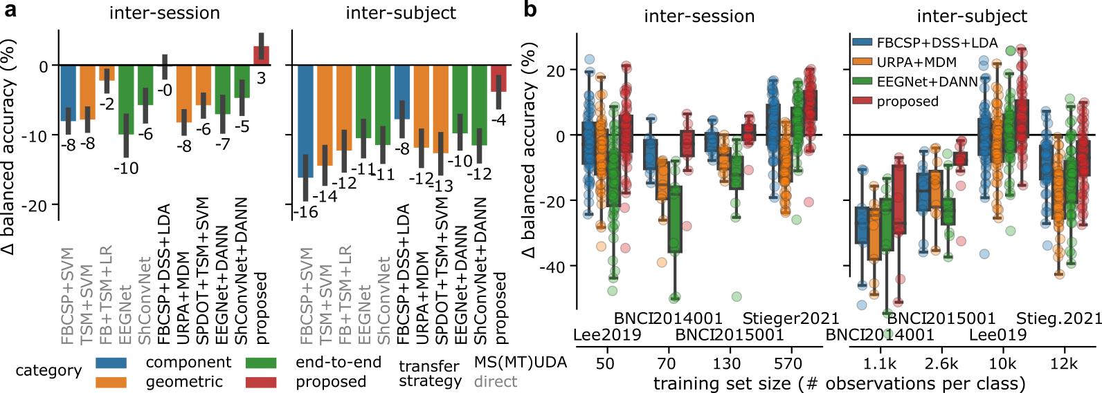
Figure 2: Mental imagery results (5 datasets). BCI test set score (balanced accuracy) for inter-session/-subject transfer learning methods relative to a SoA domain-specific reference model (80%/20% chronological train/test split; for details see appendix A.2.4). a, Barplots summarize the grand average (573 sessions, 138 subjects) results. Errorbars indicate bootstrapped (1e3 repetitions) 95% confidence intervals (over subjects). b, Box and scatter plots summarize the dataset-specific results for selected methods from each category. Datasets are ordered according to the training set size. Each dot summarizes the score for one subject. Lehner2021 is not displayed as it contains only 1 subject.

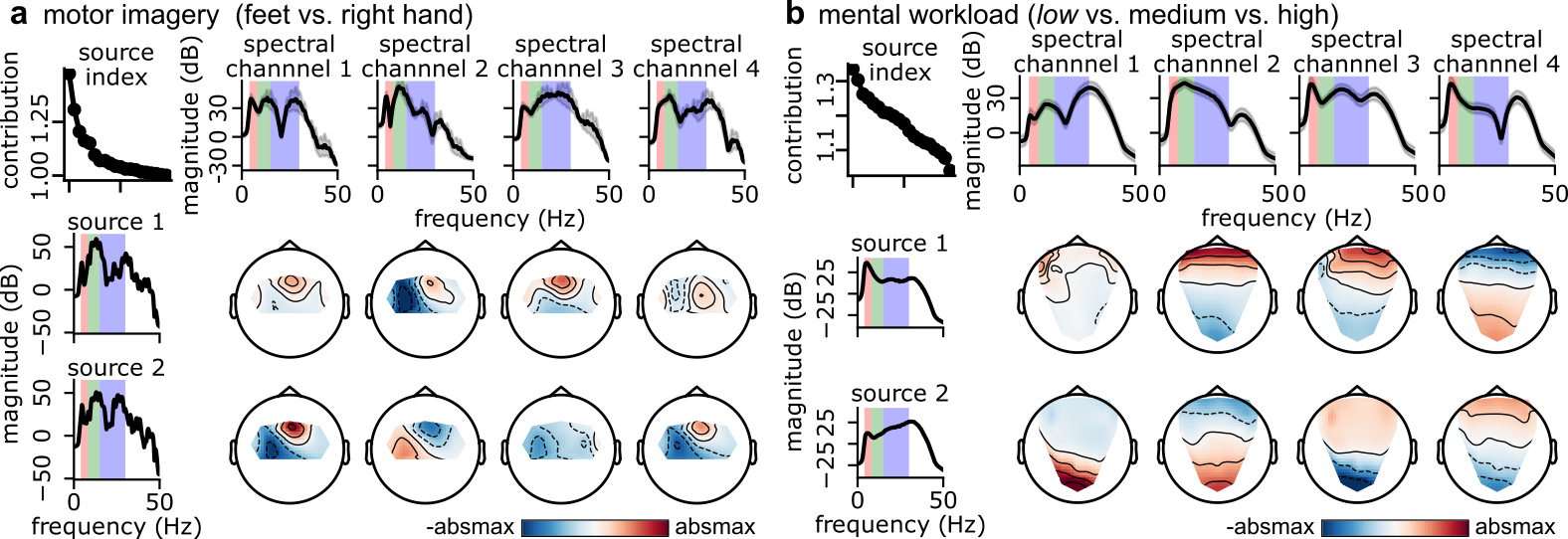
Figure 3: Model interpretation results. Patterns extracted from a TSMNet. a, Motor imagery dataset (BNCI2015001, inter-subject TL). The top, left panel lists the contribution, defined in (21), for each extracted source $k=1,...,20$ (x-axis) to the target class. Panels in the left column summarize the spectral patterns of extracted sources. For visualization purposes, only the 2 most discriminative sources are displayed. Panels in the top row summarize the frequency profile of each spectral channel (output of 4 temporal convolution layers in $f_{\theta}$). Topographic plots summarize how the source activity is projected to regions covered by the EEG channels (rows correspond to the source index; columns to spectral channels). EEG channels at darker blue or red areas capture more source activity and are, therefore, more discriminative. b, As in a for the mental workload estimation dataset and class low.

DSBN on $\mathcal{S}_{D}^{+}$ drives the success of TSMNet

Since TSMNet combines several advances, we present the results of an ablation study in Table 2. It summarizes the grand average inter-session TL test scores relative to TSMNet with SPDDSMBN for n = 138 subjects. We observed three significant effects. The largest effect can be attributed to $\mathcal{S}_{D}^{+}$, as we observed the largest performance decline if the architecture would be modified to omit the SPD manifold (4.5% with DSBN, 3% w/o DSBN). The performance gain comes at the cost of a 2.6x longer time to fit the parameters. The second largest effect can be attributed to DSBN; without DSBN the performance dropped by 3.9% (with $\mathcal{S}_{D}^{+}$) and 2.4% (w/o $\mathcal{S}_{D}^{+}$). The smallest, yet significant effect can be attributed to SPDMBN.

Table 2: Ablation study. Grand average (5 mental imagery datasets, 138 subjects, inter-session TL) score for the test data relative to the proposed method, and training fit time (50 epochs). Standard-deviation is used to report the variability across subjects. Permutation t-tests (1e4 perms, df=137, 4 tests with t-max adjustment) were used to identify significant effects.

			$\Delta$ balanced accuracy (%)		fit time (s)
			mean (std)	t-val (p-val)	mean (std)
$\mathcal{S}_{D}^{+}$	DSBN	BN method
yes	yes	SPDMBN (algo. 1) (proposed)	-	-	16.90(01.0)
	yes	SPDBN [46]	-1.60(02.2)	-7.80(0.0001)	20.30(01.6)
	no	SPDMBN (algo. 1)	-3.90(04.4)	-10.70(0.0001)	11.30(00.5)
no	yes	MBN [32]	-4.50(03.8)	-10.10(0.0001)	06.60(00.2)
	no	MBN [32]	-6.90(04.8)	-13.40(0.0001)	04.40(00.1)

5.2 Mental workload estimation

Compared to the baseline methods, TSMNet obtained the highest average scores of 54.7% (7.3%) and 52.4% (8.8%) in inter-session and -subject TL (for details see appendix A.3.1). Interestingly, the inter-session TL score of TSMNet matches the score (54.3%) of the winning method in last year’s competition [15]. To shed light on the sources utilized by TSMNet, we show patterns for a fitted model in Figure 3b. For the low mental workload class, the top contributing source’s activity peaked in the theta band and originated in pre-frontal areas. The second source’s activity originated in occipital cortex with non-focal spectral profile. Our results agree with the findings of previous research, as both areas and the theta band have been implicated in mind wandering and effort withdrawal [60].

6 Discussion

In this contribution, we proposed a machine learning framework around (domain-specific) momentum batch normalization on $\mathcal{S}_{D}^{+}$ to learn tangent space mapping (TSM) and feature extractors in an end-to-end fashion. In a theoretical analysis, we provided error bounds for the running estimate of the Fréchet mean as well as convergence guarantees under reasonable assumptions. We then applied the framework, to a multi-source multi-target unsupervised domain adaptation problem, namely, inter-session and -subject transfer learning for EEG data and obtained or attained state-of-the art performance with a simple, intrinsically interpretable model, denoted TSMNet, in a total of 6 diverse BCI datasets (138 human subjects, 573 sessions). In the case of mental imagery, we found that TSMNet significantly reduced (inter-subject TL) or even exceeded (inter-session TL) the performance gap to a SoA domain-specific method.

Although our framework could be readily extended to online UDA for unseen target domains, we limited this study to offline evaluations and leave actual BCI studies to future work. A limitation of our framework, and also any other method that involves eigen decomposition, is the computational complexity, which limits its application to high-dimensional SPD features (e.g., fMRI connectivity matrices with fine spatial granularity). Altogether, the presented results demonstrate the utility of our framework and in particular TSMNet as it not only achieves highly competitive results but is also intrinsically interpretable. While we do not foresee any immediate negative societal impacts, we provide direct contributions towards the scalability and acceptability of EEG-based healthcare [1, 5] and consumer [18, 60] technologies. We expect future works to evaluate the impact of the proposed methods in clinical applications of EEG like sleep staging [80, 81], seizure [82] or pathology detection [83, 84].

Checklist

1. For all authors…

   1. Do the main claims made in the abstract and introduction accurately reflect the paper’s contributions and scope? [Yes]

   2. Did you describe the limitations of your work? [Yes] See section 6

   3. Did you discuss any potential negative societal impacts of your work? [Yes] See section 6

   4. Have you read the ethics review guidelines and ensured that your paper conforms to them? [Yes]

2. If you are including theoretical results…

   1. Did you state the full set of assumptions of all theoretical results? [Yes] See paragraph 4 in section 3.

   2. Did you include complete proofs of all theoretical results? [Yes] See appendix A.1 in the supplementary material.

3. If you ran experiments…

   1. Did you include the code, data, and instructions needed to reproduce the main experimental results (either in the supplemental material or as a URL)? [Yes] See Supplementary Material.

   2. Did you specify all the training details (e.g., data splits, hyperparameters, how they were chosen)? [Yes] See paragraph 2 in section 5 for a brief summary and appendix A.2 for details.

   3. Did you report error bars (e.g., with respect to the random seed after running experiments multiple times)? [Yes] We provide error bars with respect to the variability across sessions and subjects.

   4. Did you include the total amount of compute and the type of resources used (e.g., type of GPUs, internal cluster, or cloud provider)? [Yes] See paragraph 3 in section 5.

4. If you are using existing assets (e.g., code, data, models) or curating/releasing new assets…

   1. If your work uses existing assets, did you cite the creators? [Yes] See paragraph 1 in section 5.

   2. Did you mention the license of the assets? [Yes] See appendix A.2.1 in the Supplementary material.

   3. Did you include any new assets either in the supplemental material or as a URL? [No]

   4. Did you discuss whether and how consent was obtained from people whose data you’re using/curating? [Yes] See paragraph 1 in section 5.

   5. Did you discuss whether the data you are using/curating contains personally identifiable information or offensive content? [Yes] See paragraph 1 in section 5.

5. If you used crowdsourcing or conducted research with human subjects…

   1. Did you include the full text of instructions given to participants and screenshots, if applicable? [N/A]

   2. Did you describe any potential participant risks, with links to Institutional Review Board (IRB) approvals, if applicable? [N/A]

   3. Did you include the estimated hourly wage paid to participants and the total amount spent on participant compensation? [N/A]

Appendix A Supplementary Material

A.1 Proof of proposition 1

In the proof, we will use Theorem 2 of [50] which relates the distance between interpolated points along the geodesic $\mathbf{R}\#_{\gamma}\mathbf{S}$, connecting points $\mathbf{R}$ and $\mathbf{S}$, and point $\mathbf{T}$ to the distances between $\mathbf{R}$, $\mathbf{S}$ and $\mathbf{T}$. Formally, for all $\mathbf{R},\mathbf{S},\mathbf{T}\in\mathcal{S}_{D}^{+}$ we have

$$\delta^{2}(\mathbf{R}\#_{\gamma}\mathbf{S},\mathbf{T})\leq(1-\gamma)\delta^{2}(\mathbf{R},\mathbf{T})+\gamma\delta^{2}(\mathbf{S},\mathbf{T})-\gamma(1-\gamma)\delta^{2}(\mathbf{R},\mathbf{S})$$ (22)

As a last ingredient for the proof, we use Proposition 1 of [50], which states that for a random variable $\mathbf{U}$, following distribution $P_{\mathcal{U}}$ defined on $\mathcal{S}_{D}^{+}$ with Fréchet mean $\mathbf{G}_{\mathcal{U}}$, we have for any point $\mathbf{V}\in\mathcal{S}_{D}^{+}$:

$$\mathbb{E}\{\delta^{2}(\mathbf{U},\mathbf{V})\}\geq\underbrace{\int\delta^{2}(\mathbf{u},\mathbf{G}_{\mathcal{U}})dP_{\mathcal{U}}(\mathbf{u})}_{=:\mathrm{Var}(\mathbf{U})}+\delta^{2}(\mathbf{V},\mathbf{G}_{\mathcal{U}})$$ (23)

which means that the expected distance between $\mathbf{V}$ and $\mathbf{U}$ is bounded from below by the variance of $\mathbf{U}$ and the distance between $\mathbf{V}$ and its Fréchet mean $\mathbf{G}_{\mathcal{U}}$.

Let us quickly repeat the definitions, assumptions and proposition 1. We define a dataset containing the latent representations generated with feature set $\theta_{k}$ as $\mathcal{Z}_{\theta_{k}}=\{f_{\theta_{k}}(\mathbf{x})|\mathbf{x}\in\mathcal{T}\}$, and a minibatch of $M$ iid samples drawn from $\mathcal{Z}_{\theta_{k}}$ at training step $k$ as $\mathcal{B}_{k}$. We denote the Fréchet mean of $\mathcal{Z}_{\theta_{k}}$ as $\mathbf{G}_{\theta_{k}}$, the estimated Fréchet mean, defined in (9), as $\mathbf{G}_{k}$, and the estimated batch mean as $\mathbf{B}_{k}$. Since the batches are drawn randomly, we consider $\mathbf{B}_{k}$ and $\mathbf{G}_{k}$ as random variables.

We assume that the variance $\mathrm{Var}_{\theta_{k}}(\mathbf{B}_{k-1})=\mathbb{E}_{\mathbf{B}_{k-1}}\{\delta^{2}(\mathbf{B}_{k-1},\mathbf{G}_{\theta_{k}})\}$ of the previous batch mean $\mathbf{B}_{k-1}$ with respect to the current Fréchet mean $\mathbf{G}_{\theta_{k}}$ is bounded by the current variance $\mathrm{Var}_{\theta_{k}}(\mathbf{B}_{k})$ and the norm of the difference in the parameters

$$\mathrm{Var}_{\theta_{k}}(\mathbf{B}_{k-1})\leq(1+||\theta_{k}-\theta_{k-1}||)\mathrm{Var}_{\theta_{k}}(\mathbf{B}_{k})$$ (24)

Proposition 1 states then that the variance of the running mean $\mathrm{Var}_{\theta_{k}}(\mathbf{G}_{k})$ is bounded by

$$\mathrm{Var}_{\theta_{k}}(\mathbf{G}_{k})\leq\mathrm{Var}_{\theta_{k}}(\mathbf{B}_{k})$$ (25)

over training steps $k$, if

$$||\theta_{k}-\theta_{k-1}||\leq\frac{1-\gamma^{2}}{(1-\gamma)^{2}}-1$$ (26)

holds true.

Proof of Proposition 1.

We prove Proposition 1 via induction. We assume that the variance $\mathrm{Var}_{\theta_{k}}(\mathbf{G}_{k-1})$, that is the expected distance between the running mean $\mathbf{G}_{k-1}$ and the Fréchet mean $\mathbf{G}_{\theta_{k}}$, is bounded by the variance of the batch mean $\mathbf{B}_{k-1}$:

$$\mathrm{Var}_{\theta_{k}}(\mathbf{G}_{k-1})=\mathbb{E}_{\mathbf{G}_{k-1}}\{\delta^{2}(\mathbf{G}_{k-1},\mathbf{G}_{\theta_{k}})\}\leq\mathrm{Var}_{\theta_{k}}(\mathbf{B}_{k-1})$$ (27)

and show that this also holds for $\mathbf{G}_{k}$ and $\mathbf{B}_{k}$. The assumption is trivially satisfied for $\mathbf{G}_{0}=\mathbf{B}_{0}$. We start the induction step with (22) and apply it to the update rule for the running estimate $\mathbf{G}_{k}$. As a result, we have

$$\delta^{2}(\mathbf{G}_{k},\mathbf{G}_{\theta_{k}})\leq(1-\gamma)\delta^{2}(\mathbf{G}_{k-1},\mathbf{G}_{\theta_{k}})+\gamma\delta^{2}(\mathbf{B}_{k},\mathbf{G}_{\theta_{k}})-\gamma(1-\gamma)\delta^{2}(\mathbf{G}_{k-1},\mathbf{B}_{k})$$ (28)

where we used $\mathbf{G}_{k}=\mathbf{G}_{k-1}\#_{\gamma}\mathbf{B}_{k}$, as defined in algorithm 1. Taking the expectations for the random variables $\mathbf{G}_{k}$, $\mathbf{G}_{k-1}$ and $\mathbf{B}_{k}$, we get

$$\mathrm{Var}_{\theta_{k}}(\mathbf{G}_{k})\leq(1-\gamma)\mathrm{Var}_{\theta_{k}}(\mathbf{G}_{k-1})+\gamma\mathrm{Var}_{\theta_{k}}(\mathbf{B}_{k})-\gamma(1-\gamma)\mathbb{E}_{\mathbf{G}_{k-1}}\{\mathbb{E}_{\mathbf{B}_{k}}\{\delta^{2}(\mathbf{G}_{k-1},\mathbf{B}_{k})\}\}$$ (29)

Using (23) to simplify the last term, we obtain

$$\mathrm{Var}_{\theta_{k}}(\mathbf{G}_{k}) \leq(1-\gamma)\mathrm{Var}_{\theta_{k}}(\mathbf{G}_{k-1})+\gamma\mathrm{Var}_{\theta_{k}}(\mathbf{B}_{k})-\gamma(1-\gamma)\left(\mathrm{Var}_{\theta_{k}}(\mathbf{G}_{k-1})+\mathrm{Var}_{\theta_{k}}(\mathbf{B}_{k})\right)$$ (30)

$$\leq(1-\gamma)^{2}\mathrm{Var}_{\theta_{k}}(\mathbf{G}_{k-1})+\gamma^{2}\mathrm{Var}_{\theta_{k}}(\mathbf{B}_{k})$$ (31)

Applying assumptions (27) and (24), we get

$$\mathrm{Var}_{\theta_{k}}(\mathbf{G}_{k}) \overset{(\ref{eq:proof:assumption})}{\leq}(1-\gamma)^{2}\mathrm{Var}_{\theta_{k}}(\mathbf{B}_{k-1})+\gamma^{2}\mathrm{Var}_{\theta_{k}}(\mathbf{B}_{k})$$ (32)

$$\overset{(\ref{eq:proof:assumption1})}{\leq}\left[(1-\gamma)^{2}(1+||\theta_{k}-\theta_{k-1}||)+\gamma^{2}\right]\mathrm{Var}_{\theta_{k}}(\mathbf{B}_{k})$$ (33)

The resulting inequality holds true, for

$$(1-\gamma)^{2}(1+||\theta_{k}-\theta_{k-1}||)+\gamma^{2}\overset{!}{\leq}1\Leftrightarrow||\theta_{k}-\theta_{k-1}||\overset{!}{\leq}\frac{1-\gamma^{2}}{(1-\gamma)^{2}}-1$$ (34)

and, in turn, results in feasible bounds for the parameter updates for fixed $\gamma\in(0,1)$. This concludes the proof. ∎

A.2 Supplementary Methods

A.2.1 Datasets

A summary of the datasets’ key attributes is listed in Table 3. The datasets contain a diverse sample of 154 human subjects, whose data was acquired in Europe (38 subjects; BNCI2014001,BNCI2015001,Lehner2021,Hehenberger2021,Hinss2021), Asia (54 subjects; Lee2019) and North America (62 subjects; Stieger2021).

Table 3: Dataset attributes. The epoch indices the temporal window after a task cue (time relative to cue onset) that was extracted from continuous EEG data.

	epoch	sampling	channels	subjects	sessions	obsevations
dataset	(s)	rate (Hz)	#	#	#	# (per session)
BNCI2014001	0.5 - 3.5	250	22	9	2	288
BNCI2015001	1.0 - 4.0	256	13	12	2-3	200
Lee2019	1.0 - 3.5	250	20	54	2	100
Stieger2021	1.0 - 3.0	250	34	62	4-8	390
Lehner2021	0.5 - 2.5	250	60	1	7	61
Hehenberger2021	1.0 - 3.0	250	32	1	26	105
Hinss2021	0.0 - 2.0	250	30	15	2	447

	classes	license	identifier	linked
dataset #				publication
BNCI2014001	4	CC BY-ND 4.0	001-2014	[63]
BNCI2015001	2	CC BY-NC-ND 4.0	001-2015	[64]
Lee2019	2	unspecified	100542	[65]
Stieger2021	4	CC BY 4.0	m9.figshare.13123148.v1	[67]
Lehner2021	2	InC-NC	10.3929/ethz-b-000458693	[66]
Hehenberger2021	4	individual	-	[68]
Hinss2021	3	CC BY-SA 4.0	10.5281/zenodo.5055046	[69]

A.2.2 Preprocessing

Depending on the dataset, either all or a subset of EEG channels was selected, and then resampled along the temporal dimension to a sampling rate of either 250 or 256 Hz. (see Table 3). Thereafter, an infinite impulse response (IIR) bandpass filter was used to extract EEG activity in the 4 to 36 Hz range (4th order Butterworth filter, 4 and 36 Hz cut-off frequencies, zero-phase). Some baseline methods required spectrally resolved input data. For these, we applied a bank of 8 filters with similar parameters except for the cut-off frequencies ([4, 8], [8, 12], …, [32, 36] Hz). Finally, short epochs (=segments) were extracted (see Table 3) relative to the task cues (=labels). The labeled data were then extended with a domain index (= unique integer associated to one session of one subject).

A.2.3 Baseline methods

We considered several established and SoA baseline methods which were previously applied to inter-session/-subject TL. They can be broadly categorized as component based, Riemannian geometry aware or deep learning which we denote component, geometric and end-to-end, respectively. For the component category, we considered the popular filter-bank common spatial patterns (FBCSP+SVM) [71] and a variant [68], designed for MSMTUDA, that applies domain-specific standardization (DSS) to features before classification, denoted FBCSP+DSS+LDA. The geometric category was represented by TSM+SVM [12], a spectrally resolved variant [17] denoted FB+TSM+LR (which was also used as domain-specific baseline method). We additionally considered two MSUDA methods, denoted URPA+MDM and SPDOT+TSM+SVM here, that align SPD observations (=spatial covariance matrices) of different domains. The former uses Riemannian Procrustes Analysis (RPA) [30] to align domains, and the latter optimal transport (OT) on $\mathcal{S}^{+}_{D}$ [72]. The end-to-end category was represented by EEGNet [73] and ShConvNet [56] two convolutional neural network architectures specifically designed for EEG data. We additionally considered variants [25] that use domain-adversarial neural networks (DANN) [85] to learn domain-invariant latent representations.

A.2.4 Domain-specific reference method

Due to the success of TSM models [14, 10], we considered a spectrally resolved model [13, 17] which consisted of a filter-bank to separate activity of canonical frequency bands. For each frequency band, PCA was used to reduce the spatial dimensionality and TSM to project the SPD features to the Euclidean vector space. Finally, all features were pooled and submitted to a penalized logistic regression classifier. For further details, see [17].

A.2.5 TSMNet

Architecture

The architecture of TSMNet is outlined in Figure 4 and detailed in Table 4. The feature extractor $f_{\theta}$ comprises two convolutional layers, followed by covariance pooling [57], BiMap [37] and ReEig [37] layers. The first convolutional layer performs convolution along the temporal dimension; implementing a finite impulse response (FIR) filter bank (4 filters) with learnable parameters. The second convolutional layer applies spatio-spectral filters (40 filters) along the spatial and convolutional channel dimensions. Covariance pooling is then applied along the temporal dimension. A subsequent BiMap layer projects covariance matrices to a subspace via a bilinear mapping (i.e, $\mathrm{BiMap}(\mathbf{Z})=\mathbf{W}^{T}_{\theta}\mathbf{Z}\mathbf{W}_{\theta}$) where the parameter matrix $\mathbf{W}_{\theta}$ is constrained to have orthogonal rows (i.e., $\mathbf{W}_{\theta}\in\{\mathbf{U}\in\mathbb{R}^{I\times O}:\mathbf{U}^{T}\mathbf{U}=\mathbf{I}_{O},I\geq O\}$). Next, a ReEig layer rectifies all eigenvalues, lower than a threshold $\epsilon=10^{-4}$ (i.e, $\mathrm{ReEig}(\mathbf{Z})=\mathbf{U}\mathrm{max}(\mathbf{\Sigma},\epsilon\mathbf{I})\mathbf{U}^{T}$ with $[\mathbf{\Sigma},\mathbf{U}]=\mathrm{eig}(\mathbf{Z})$).
Domain-specific tangent space mapping $m_{\phi}$ is implemented via combining SPDDSMBN and LogEig layers. In order for $m_{\phi}$ to align the domain data and compute TSM, we use SPDDSMBN (18) with shared parameters (i.e., $\mathbf{G}_{\phi_{i}}=\mathbf{G}_{\phi}=\mathbf{I},\nu_{\phi_{i}}=\nu_{\phi}$) in (16). The classifier $g_{\psi}$ was parametrized as a linear layer with softmax activations.

Parameter estimation

We used the cross entropy loss as training objective, and the standard backpropagation framework with extensions for structured matrices [49] and manifold-constrained gradients [40] to propagate gradients through the layers of TSMNet. Gradients were estimated with mini-batches of fixed size (50 observations; 10 per domain; 5 distinct domains) and converted into parameter updates with the Riemannian ADAM optimizer [58] ($10^{-3}$ learning rate, $10^{-4}$ weight decay applied to unconstrained parameters; $\beta_{1}=0.9,\beta_{2}=0.999$).

For every MSMTUDA problem, comprising source and target domain sets, we split the source domains’ data into training and validation sets (80%/20% splits; randomized; stratified across domains and labels) and repeatedly iterated through the training set for 50 epochs via exhaustive minibatch sampling. As required by SPDMBN, we implemented a decaying schedule (over epochs) for the training momentum parameter $\gamma_{train}(k)$, defined in (11), with $\gamma_{train}(0)=1$ and $\gamma_{min}=0.2$ attained at epoch $K=40$. During training, we monitored the loss on the validation data (at the end of every epoch). Post training, the model with minimal loss on the validation data was selected. For each target domain, the associated data was then passed through this model to estimate the labels. During the forward pass, the domain’s normalization statistics within the SPDMBN layers were computed by solving (4) with the Karcher flow algorithm [42].

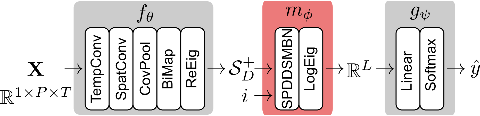
Figure 4: Overview of the TSMNet architecture. The network uses observations $\mathbf{X}$ and the associated domain index $i$ to estimate the target label $\hat{y}$.

Table 4: TSMNet architecture details. The letters P, T and C refer to the number of input channels, temporal samples and classes.

Block	Input (dim)	Output (dim)	Parameter (dim)	Operation	Note
TempConv	1 x P x T	4 x P x T	4 x 1 x 1 x 25	convolution	padding: same, reflect
SpatConv	4 x P x T	40 x 1 x T	40 x 4 x P x 1	convolution	padding: valid
CovPool	40 x T	40 x 40		covariance	temporal dimension
BiMap	40 x 40	20 x 20	40 x 20	bilinear	subspace projection
ReEig	20 x 20	20 x 20		EV threshold	threshold = 0.0001
SPDDSMBN	20 x 20	20 x 20	1	TSM	domain alignment
LogEig	20 x 20	210		TSM
Linear	210	C	211 x C	linear	softmax activation

A.3 Supplementary results

A.3.1 EEG data

The test set score for each considered EEG dataset is summarized in in Table 5. Significant differences between the proposed method (TSMNet with SPDDSMBN) and baseline methods are highlighted.

Table 5: Average (standard deviation across sessions or subjects) test set score (balanced accuracy; higher is better) for all BCI datasets and evaluations. Permutation-paired t-test were used to identify significant differences between the proposed (highlighted) and baseline methods (1e4 permutations, 10 tests, tmax correction). Significant differences are highlighted ($\mathbin{\vbox{\hbox{\scalebox{0.5}{$\bullet$}}}}$ $p\leq 0.05$, $\mathbin{\vbox{\hbox{\scalebox{0.75}{$\bullet$}}}}$ $p\leq 0.01$, $\mathbin{\vbox{\hbox{\scalebox{1.0}{$\bullet$}}}}$ $p\leq 0.001$).

	dataset	BNCI2014001		BNCI2015001
	evaluation	inter-session	inter-subject	inter-session	inter-subject
	degrees of freedom / # classes	17 / 4	8 / 4	27 / 2	11 / 2
UDA	method
no	FBCSP+SVM	$\mathbin{\vbox{\hbox{\scalebox{0.5}{$\bullet$}}}}$ 60.60(04.9)	$\mathbin{\vbox{\hbox{\scalebox{0.5}{$\bullet$}}}}$ 32.30(07.3)	$\mathbin{\vbox{\hbox{\scalebox{0.75}{$\bullet$}}}}$ 81.50(04.4)	$\mathbin{\vbox{\hbox{\scalebox{0.75}{$\bullet$}}}}$ 58.60(13.4)
	TSM+SVM	$\mathbin{\vbox{\hbox{\scalebox{0.75}{$\bullet$}}}}$ 61.80(04.1)	$\mathbin{\vbox{\hbox{\scalebox{0.5}{$\bullet$}}}}$ 34.70(08.6)	$\mathbin{\vbox{\hbox{\scalebox{1.0}{$\bullet$}}}}$ 75.70(05.1)	$\mathbin{\vbox{\hbox{\scalebox{1.0}{$\bullet$}}}}$ 56.00(06.0)
	FB+TSM+LR	069.80(04.8)	$\mathbin{\vbox{\hbox{\scalebox{0.5}{$\bullet$}}}}$ 36.50(08.2)	$\mathbin{\vbox{\hbox{\scalebox{0.5}{$\bullet$}}}}$ 80.90(06.0)	$\mathbin{\vbox{\hbox{\scalebox{0.75}{$\bullet$}}}}$ 60.60(10.9)
	EEGNet	$\mathbin{\vbox{\hbox{\scalebox{1.0}{$\bullet$}}}}$ 41.80(05.8)	$\mathbin{\vbox{\hbox{\scalebox{0.5}{$\bullet$}}}}$ 43.30(17.0)	$\mathbin{\vbox{\hbox{\scalebox{1.0}{$\bullet$}}}}$ 72.40(08.4)	$\mathbin{\vbox{\hbox{\scalebox{1.0}{$\bullet$}}}}$ 59.20(09.5)
	ShConvNet	$\mathbin{\vbox{\hbox{\scalebox{1.0}{$\bullet$}}}}$ 51.30(02.3)	$\mathbin{\vbox{\hbox{\scalebox{0.5}{$\bullet$}}}}$ 42.20(16.2)	$\mathbin{\vbox{\hbox{\scalebox{1.0}{$\bullet$}}}}$ 74.10(04.2)	$\mathbin{\vbox{\hbox{\scalebox{1.0}{$\bullet$}}}}$ 58.70(05.8)
yes	FBCSP+DSS+LDA	071.30(01.8)	048.30(14.3)	084.60(04.8)	$\mathbin{\vbox{\hbox{\scalebox{0.75}{$\bullet$}}}}$ 67.70(14.3)
	URPA+MDM	$\mathbin{\vbox{\hbox{\scalebox{1.0}{$\bullet$}}}}$ 59.50(02.7)	046.80(14.6)	$\mathbin{\vbox{\hbox{\scalebox{1.0}{$\bullet$}}}}$ 79.20(04.6)	$\mathbin{\vbox{\hbox{\scalebox{0.75}{$\bullet$}}}}$ 70.30(16.1)
	SPDOT+TSM+SVM	066.80(03.8)	$\mathbin{\vbox{\hbox{\scalebox{0.5}{$\bullet$}}}}$ 38.60(08.6)	$\mathbin{\vbox{\hbox{\scalebox{1.0}{$\bullet$}}}}$ 77.50(02.9)	$\mathbin{\vbox{\hbox{\scalebox{1.0}{$\bullet$}}}}$ 63.30(08.1)
	EEGNet+DANN	$\mathbin{\vbox{\hbox{\scalebox{1.0}{$\bullet$}}}}$ 50.00(07.7)	045.80(18.0)	$\mathbin{\vbox{\hbox{\scalebox{1.0}{$\bullet$}}}}$ 71.60(05.3)	$\mathbin{\vbox{\hbox{\scalebox{1.0}{$\bullet$}}}}$ 63.70(11.1)
	ShConvNet+DANN	$\mathbin{\vbox{\hbox{\scalebox{1.0}{$\bullet$}}}}$ 51.60(03.2)	$\mathbin{\vbox{\hbox{\scalebox{0.5}{$\bullet$}}}}$ 42.20(13.6)	$\mathbin{\vbox{\hbox{\scalebox{1.0}{$\bullet$}}}}$ 74.10(04.0)	$\mathbin{\vbox{\hbox{\scalebox{1.0}{$\bullet$}}}}$ 64.20(11.6)
	TSMNet(SPDDSMBN)	069.00(03.6)	051.60(16.5)	085.80(04.3)	077.00(13.7)
	dataset	Lee2019		Stieger2021
	evaluation	inter-session	inter-subject	inter-session	inter-subject
	degrees of freedom / # classes	107 / 2	53 / 2	411 / 4	61 / 4
UDA	method
no	FBCSP+SVM	$\mathbin{\vbox{\hbox{\scalebox{1.0}{$\bullet$}}}}$ 63.10(04.2)	$\mathbin{\vbox{\hbox{\scalebox{1.0}{$\bullet$}}}}$ 63.40(12.1)	$\mathbin{\vbox{\hbox{\scalebox{1.0}{$\bullet$}}}}$ 47.50(07.0)	$\mathbin{\vbox{\hbox{\scalebox{1.0}{$\bullet$}}}}$ 37.60(10.5)
	TSM+SVM	$\mathbin{\vbox{\hbox{\scalebox{1.0}{$\bullet$}}}}$ 62.50(03.3)	$\mathbin{\vbox{\hbox{\scalebox{1.0}{$\bullet$}}}}$ 65.30(13.0)	$\mathbin{\vbox{\hbox{\scalebox{1.0}{$\bullet$}}}}$ 49.50(08.1)	$\mathbin{\vbox{\hbox{\scalebox{1.0}{$\bullet$}}}}$ 40.20(12.3)
	FB+TSM+LR	$\mathbin{\vbox{\hbox{\scalebox{0.75}{$\bullet$}}}}$ 65.20(04.5)	$\mathbin{\vbox{\hbox{\scalebox{1.0}{$\bullet$}}}}$ 68.50(12.4)	$\mathbin{\vbox{\hbox{\scalebox{1.0}{$\bullet$}}}}$ 57.30(07.3)	$\mathbin{\vbox{\hbox{\scalebox{1.0}{$\bullet$}}}}$ 40.30(09.2)
	EEGNet	$\mathbin{\vbox{\hbox{\scalebox{1.0}{$\bullet$}}}}$ 51.20(02.7)	$\mathbin{\vbox{\hbox{\scalebox{1.0}{$\bullet$}}}}$ 69.60(13.8)	$\mathbin{\vbox{\hbox{\scalebox{1.0}{$\bullet$}}}}$ 58.30(07.9)	$\mathbin{\vbox{\hbox{\scalebox{0.75}{$\bullet$}}}}$ 43.10(11.0)
	ShConvNet	$\mathbin{\vbox{\hbox{\scalebox{1.0}{$\bullet$}}}}$ 57.80(04.0)	$\mathbin{\vbox{\hbox{\scalebox{1.0}{$\bullet$}}}}$ 68.50(13.6)	$\mathbin{\vbox{\hbox{\scalebox{1.0}{$\bullet$}}}}$ 60.10(06.6)	$\mathbin{\vbox{\hbox{\scalebox{1.0}{$\bullet$}}}}$ 42.20(10.4)
yes	FBCSP+DSS+LDA	066.80(04.1)	$\mathbin{\vbox{\hbox{\scalebox{1.0}{$\bullet$}}}}$ 68.70(13.8)	$\mathbin{\vbox{\hbox{\scalebox{1.0}{$\bullet$}}}}$ 59.40(06.6)	$\mathbin{\vbox{\hbox{\scalebox{0.75}{$\bullet$}}}}$ 48.20(13.4)
	URPA+MDM	$\mathbin{\vbox{\hbox{\scalebox{1.0}{$\bullet$}}}}$ 63.80(04.2)	$\mathbin{\vbox{\hbox{\scalebox{1.0}{$\bullet$}}}}$ 66.70(12.3)	$\mathbin{\vbox{\hbox{\scalebox{1.0}{$\bullet$}}}}$ 47.00(06.6)	$\mathbin{\vbox{\hbox{\scalebox{1.0}{$\bullet$}}}}$ 38.70(10.4)
	SPDOT+TSM+SVM	$\mathbin{\vbox{\hbox{\scalebox{0.75}{$\bullet$}}}}$ 65.60(04.2)	$\mathbin{\vbox{\hbox{\scalebox{1.0}{$\bullet$}}}}$ 65.40(10.5)	$\mathbin{\vbox{\hbox{\scalebox{1.0}{$\bullet$}}}}$ 50.30(05.8)	$\mathbin{\vbox{\hbox{\scalebox{1.0}{$\bullet$}}}}$ 42.10(10.5)
	EEGNet+DANN	$\mathbin{\vbox{\hbox{\scalebox{1.0}{$\bullet$}}}}$ 55.40(04.4)	$\mathbin{\vbox{\hbox{\scalebox{1.0}{$\bullet$}}}}$ 69.40(13.1)	$\mathbin{\vbox{\hbox{\scalebox{1.0}{$\bullet$}}}}$ 60.10(06.9)	$\mathbin{\vbox{\hbox{\scalebox{0.75}{$\bullet$}}}}$ 43.60(10.7)
	ShConvNet+DANN	$\mathbin{\vbox{\hbox{\scalebox{1.0}{$\bullet$}}}}$ 59.10(03.4)	$\mathbin{\vbox{\hbox{\scalebox{1.0}{$\bullet$}}}}$ 66.00(12.4)	$\mathbin{\vbox{\hbox{\scalebox{1.0}{$\bullet$}}}}$ 61.30(06.0)	$\mathbin{\vbox{\hbox{\scalebox{1.0}{$\bullet$}}}}$ 43.10(11.5)
	TSMNet(SPDDSMBN)	068.20(04.1)	074.60(14.2)	064.80(06.8)	048.90(14.3)
	dataset	Lehner2021	Hehen.2021	Hinss2021
	evaluation	inter-session	inter-session	inter-session	inter-subject
	degrees of freedom / # classes	6 / 2	25 / 4	29 / 3	14 / 3
UDA	method
no	FBCSP+SVM	068.90(06.0)	$\mathbin{\vbox{\hbox{\scalebox{0.75}{$\bullet$}}}}$ 52.50(07.1)	$\mathbin{\vbox{\hbox{\scalebox{0.75}{$\bullet$}}}}$ 43.70(08.2)	045.60(06.5)
	TSM+SVM	062.70(09.1)	$\mathbin{\vbox{\hbox{\scalebox{1.0}{$\bullet$}}}}$ 44.80(07.3)	$\mathbin{\vbox{\hbox{\scalebox{1.0}{$\bullet$}}}}$ 36.80(04.5)	$\mathbin{\vbox{\hbox{\scalebox{0.75}{$\bullet$}}}}$ 41.70(07.4)
	FB+TSM+LR	073.00(09.6)	$\mathbin{\vbox{\hbox{\scalebox{0.75}{$\bullet$}}}}$ 52.20(06.0)	$\mathbin{\vbox{\hbox{\scalebox{1.0}{$\bullet$}}}}$ 40.80(07.1)	$\mathbin{\vbox{\hbox{\scalebox{0.5}{$\bullet$}}}}$ 45.10(05.0)
	EEGNet	$\mathbin{\vbox{\hbox{\scalebox{0.5}{$\bullet$}}}}$ 49.60(06.4)	$\mathbin{\vbox{\hbox{\scalebox{1.0}{$\bullet$}}}}$ 48.20(06.3)	$\mathbin{\vbox{\hbox{\scalebox{0.75}{$\bullet$}}}}$ 46.30(10.1)	047.80(05.1)
	ShConvNet	$\mathbin{\vbox{\hbox{\scalebox{0.5}{$\bullet$}}}}$ 56.30(07.3)	$\mathbin{\vbox{\hbox{\scalebox{1.0}{$\bullet$}}}}$ 53.00(05.1)	048.90(07.4)	$\mathbin{\vbox{\hbox{\scalebox{0.5}{$\bullet$}}}}$ 45.90(06.8)
yes	FBCSP+DSS+LDA	077.10(08.4)	056.40(05.3)	$\mathbin{\vbox{\hbox{\scalebox{0.75}{$\bullet$}}}}$ 47.10(07.4)	048.40(09.0)
	URPA+MDM	070.80(08.2)	$\mathbin{\vbox{\hbox{\scalebox{1.0}{$\bullet$}}}}$ 46.60(07.2)	051.40(03.7)	048.40(06.1)
	SPDOT+TSM+SVM	$\mathbin{\vbox{\hbox{\scalebox{0.5}{$\bullet$}}}}$ 63.00(09.2)	$\mathbin{\vbox{\hbox{\scalebox{1.0}{$\bullet$}}}}$ 45.90(06.0)	$\mathbin{\vbox{\hbox{\scalebox{1.0}{$\bullet$}}}}$ 42.00(04.7)	$\mathbin{\vbox{\hbox{\scalebox{1.0}{$\bullet$}}}}$ 40.40(07.5)
	EEGNet+DANN	$\mathbin{\vbox{\hbox{\scalebox{0.5}{$\bullet$}}}}$ 49.80(03.7)	$\mathbin{\vbox{\hbox{\scalebox{1.0}{$\bullet$}}}}$ 49.30(06.7)	$\mathbin{\vbox{\hbox{\scalebox{0.5}{$\bullet$}}}}$ 49.40(06.8)	050.00(07.3)
	ShConvNet+DANN	$\mathbin{\vbox{\hbox{\scalebox{0.5}{$\bullet$}}}}$ 57.50(07.6)	$\mathbin{\vbox{\hbox{\scalebox{0.5}{$\bullet$}}}}$ 54.00(05.1)	051.50(04.9)	048.80(05.7)
	TSMNet(SPDDSMBN)	077.70(10.0)	057.80(05.8)	054.70(07.3)	052.40(08.8)

References

- Schomer and Lopes da Silva [2018] Donald L. Schomer and Fernando H. Lopes da Silva. Niedermeyer’s Electroencephalography: basic principles, clinical applications, and related fields. Lippincott Williams & Wilkins, 7 edition, 2018. ISBN 978-0-19-022848-4. doi: 10.1212/WNL.0b013e31822f0490.
- Pfurtscheller and Lopes [1999] G Pfurtscheller and F H Lopes. Event-related EEG / MEG synchronization and. Clinical Neurophysiology, 110:10576479, 1999.
- Faller et al. [2019] Josef Faller, Jennifer Cummings, Sameer Saproo, and Paul Sajda. Regulation of arousal via online neurofeedback improves human performance in a demanding sensory-motor task. Proceedings of the National Academy of Sciences, 116(13):6482–6490, 2019. doi: 10.1073/pnas.1817207116.
- Zhang et al. [2021] Yu Zhang, Wei Wu, Russell T. Toll, Sharon Naparstek, Adi Maron-Katz, Mallissa Watts, Joseph Gordon, Jisoo Jeong, Laura Astolfi, Emmanuel Shpigel, Parker Longwell, Kamron Sarhadi, Dawlat El-Said, Yuanqing Li, Crystal Cooper, Cherise Chin-Fatt, Martijn Arns, Madeleine S. Goodkind, Madhukar H. Trivedi, Charles R. Marmar, and Amit Etkin. Identification of psychiatric disorder subtypes from functional connectivity patterns in resting-state electroencephalography. Nature Biomedical Engineering, 5(4):309–323, 2021. doi: 10.1038/s41551-020-00614-8.
- Wolpaw et al. [2002] Jonathan R Wolpaw, Niels Birbaumer, Dennis J McFarland, Gert Pfurtscheller, and Theresa M Vaughan. Brain-computer interfaces for communication and control. Clinical neurophysiology : official journal of the International Federation of Clinical Neurophysiology, 113:767–791, 2002. doi: doi:10.1016/s1388-2457(02)00057-3.
- Ben-David et al. [2010] Shai Ben-David, John Blitzer, Koby Crammer, Alex Kulesza, Fernando Pereira, and Jennifer Wortman Vaughan. A theory of learning from different domains. Machine Learning, 79(1-2):151–175, 2010. doi: 10.1007/s10994-009-5152-4.
- Hoffman et al. [2018] Judy Hoffman, Mehryar Mohri, and Ningshan Zhang. Algorithms and theory for multiple-source adaptation. In S. Bengio, H. Wallach, H. Larochelle, K. Grauman, N. Cesa-Bianchi, and R. Garnett, editors, Advances in Neural Information Processing Systems, volume 31. Curran Associates, Inc., 2018.
- Wu et al. [2020] Dongrui Wu, Yifan Xu, and Bao-Liang Lu. Transfer Learning for EEG-Based Brain-Computer Interfaces: A Review of Progress Made Since 2016. IEEE Transactions on Cognitive and Developmental Systems, pages 1–1, 2020. doi: 10.1109/TCDS.2020.3007453.
- Neuper et al. [2005] Christa Neuper, Reinhold Scherer, Miriam Reiner, and Gert Pfurtscheller. Imagery of motor actions: Differential effects of kinesthetic and visual–motor mode of imagery in single-trial EEG. Cognitive Brain Research, 25(3):668–677, 2005. doi: 10.1016/j.cogbrainres.2005.08.014.
- Lotte et al. [2018] F Lotte, L Bougrain, A Cichocki, M Clerc, M Congedo, A Rakotomamonjy, and F Yger. A review of classification algorithms for EEG-based brain–computer interfaces: a 10 year update. Journal of Neural Engineering, 15(3):031005, 2018. doi: 10.1088/1741-2552/aab2f2.
- Statthaler et al. [2017] Karina Statthaler, Andreas Schwarz, David Steyrl, Reinmar J. Kobler, Maria Katharina Höller, Julia Brandstetter, Lea Hehenberger, Marvin Bigga, and Gernot Müller-Putz. Cybathlon experiences of the Graz BCI racing team Mirage91 in the brain-computer interface discipline. Journal of NeuroEngineering and Rehabilitation, 14(1):129, 2017. doi: 10.1186/s12984-017-0344-9.
- Barachant et al. [2012] Alexandre Barachant, Stéphane Bonnet, Marco Congedo, and Christian Jutten. Multiclass brain-computer interface classification by Riemannian geometry. IEEE transactions on bio-medical engineering, 59(4):920–928, 2012. doi: 10.1109/TBME.2011.2172210.
- Sabbagh et al. [2019] David Sabbagh, Pierre Ablin, Gaël Varoquaux, Alexandre Gramfort, and Denis A Engemann. Manifold-regression to predict from MEG/EEG brain signals without source modeling. In Advances in Neural Information Processing Systems, pages 7323–7334, 2019.
- Jayaram and Barachant [2018] Vinay Jayaram and Alexandre Barachant. MOABB: trustworthy algorithm benchmarking for BCIs. Journal of Neural Engineering, 15(6):066011, 2018. doi: 10.1088/1741-2552/aadea0.
- Roy et al. [2022] Raphaëlle N. Roy, Marcel F. Hinss, Ludovic Darmet, Simon Ladouce, Emilie S. Jahanpour, Bertille Somon, Xiaoqi Xu, Nicolas Drougard, Frédéric Dehais, and Fabien Lotte. Retrospective on the First Passive Brain-Computer Interface Competition on Cross-Session Workload Estimation. Frontiers in Neuroergonomics, 3:838342, 2022. doi: 10.3389/fnrgo.2022.838342.
- Congedo et al. [2017] Marco Congedo, Alexandre Barachant, and Rajendra Bhatia. Riemannian geometry for EEG-based brain-computer interfaces; a primer and a review. Brain-Computer Interfaces, 4(3):155–174, 2017. doi: 10.1080/2326263X.2017.1297192.
- Kobler et al. [2021] Reinmar J. Kobler, Jun-Ichiro Hirayama, Lea Hehenberger, Catarina Lopes-Dias, Gernot Müller-Putz, and Motoaki Kawanabe. On the interpretation of linear Riemannian tangent space model parameters in M/EEG. In Proceedings of the 43rd Annual International Conference of the IEEE Engineering in Medicine and Biology Society (EMBC). IEEE, 2021. doi: 10.1109/EMBC46164.2021.9630144.
- Fairclough and Lotte [2020] Stephen H. Fairclough and Fabien Lotte. Grand Challenges in Neurotechnology and System Neuroergonomics. Frontiers in Neuroergonomics, 1:602504, 2020. doi: 10.3389/fnrgo.2020.602504.
- Wei et al. [2022] Xiaoxi Wei, A. Aldo Faisal, Moritz Grosse-Wentrup, Alexandre Gramfort, Sylvain Chevallier, Vinay Jayaram, Camille Jeunet, Stylianos Bakas, Siegfried Ludwig, Konstantinos Barmpas, Mehdi Bahri, Yannis Panagakis, Nikolaos Laskaris, Dimitrios A. Adamos, Stefanos Zafeiriou, William C. Duong, Stephen M. Gordon, Vernon J. Lawhern, Maciej Śliwowski, Vincent Rouanne, and Piotr Tempczyk. 2021 BEETL Competition: Advancing Transfer Learning for Subject Independence & Heterogenous EEG Data Sets. arXiv:2202.12950 [cs, eess], 2022.
- Jayaram et al. [2016] Vinay Jayaram, Morteza Alamgir, Yasemin Altun, Bernhard Scholkopf, and Moritz Grosse-Wentrup. Transfer Learning in Brain-Computer Interfaces. IEEE Computational Intelligence Magazine, 11(1):20–31, 2016. doi: 10.1109/MCI.2015.2501545.
- Fazli et al. [2009] Siamac Fazli, Florin Popescu, Márton Danóczy, Benjamin Blankertz, Klaus-Robert Müller, and Cristian Grozea. Subject-independent mental state classification in single trials. Neural Networks, 22(9):1305–1312, 2009. doi: 10.1016/j.neunet.2009.06.003.
- Samek et al. [2014] Wojciech Samek, Motoaki Kawanabe, and Klaus Robert Müller. Divergence-based framework for common spatial patterns algorithms. IEEE Reviews in Biomedical Engineering, 7:50–72, 2014. doi: 10.1109/RBME.2013.2290621.
- Kwon et al. [2020] O-Yeon Kwon, Min-Ho Lee, Cuntai Guan, and Seong-Whan Lee. Subject-Independent Brain–Computer Interfaces Based on Deep Convolutional Neural Networks. IEEE Transactions on Neural Networks and Learning Systems, 31(10):3839–3852, 2020. doi: 10.1109/TNNLS.2019.2946869.
- Zhao et al. [2020] Sicheng Zhao, Bo Li, Colorado Reed, Pengfei Xu, and Kurt Keutzer. Multi-source Domain Adaptation in the Deep Learning Era: A Systematic Survey, 2020.
- Ozdenizci et al. [2020] Ozan Ozdenizci, Ye Wang, Toshiaki Koike-Akino, and Deniz Erdogmus. Learning Invariant Representations From EEG via Adversarial Inference. IEEE Access, 8:27074–27085, 2020. doi: 10.1109/ACCESS.2020.2971600.
- Xu et al. [2021] Lichao Xu, Zhen Ma, Jiayuan Meng, Minpeng Xu, Tzyy-Ping Jung, and Dong Ming. Improving Transfer Performance of Deep Learning with Adaptive Batch Normalization for Brain-computer Interfaces . In 2021 43rd Annual International Conference of the IEEE Engineering in Medicine & Biology Society (EMBC), pages 5800–5803, Mexico, 2021. IEEE. ISBN 978-1-72811-179-7. doi: 10.1109/EMBC46164.2021.9629529.
- Xu et al. [2020] Lichao Xu, Minpeng Xu, Yufeng Ke, Xingwei An, Shuang Liu, and Dong Ming. Cross-Dataset Variability Problem in EEG Decoding With Deep Learning. Frontiers in Human Neuroscience, 14:103, 2020. doi: 10.3389/fnhum.2020.00103.
- Mane et al. [2021] Ravikiran Mane, Effie Chew, Karen Chua, Kai Keng Ang, Neethu Robinson, A. P. Vinod, Seong-Whan Lee, and Cuntai Guan. FBCNet: A Multi-view Convolutional Neural Network for Brain-Computer Interface. arXiv:2104.01233 [cs, eess], 2021.
- Zanini et al. [2018] Paolo Zanini, Marco Congedo, Christian Jutten, Salem Said, and Yannick Berthoumieu. Transfer Learning: A Riemannian Geometry Framework With Applications to Brain–Computer Interfaces. IEEE Transactions on Biomedical Engineering, 65(5):1107–1116, 2018. doi: 10.1109/TBME.2017.2742541.
- Rodrigues et al. [2019] Pedro Luiz Coelho Rodrigues, Christian Jutten, and Marco Congedo. Riemannian Procrustes Analysis: Transfer Learning for Brain–Computer Interfaces. IEEE Transactions on Biomedical Engineering, 66(8):2390–2401, 2019. doi: 10.1109/TBME.2018.2889705.
- Yair et al. [2019] Or Yair, Mirela Ben-Chen, and Ronen Talmon. Parallel Transport on the Cone Manifold of SPD Matrices for Domain Adaptation. IEEE Transactions on Signal Processing, 67(7):1797–1811, 2019. doi: 10.1109/TSP.2019.2894801.
- Yong et al. [2020] Hongwei Yong, Jianqiang Huang, Deyu Meng, Xiansheng Hua, and Lei Zhang. Momentum Batch Normalization for Deep Learning with Small Batch Size. In Andrea Vedaldi, Horst Bischof, Thomas Brox, and Jan-Michael Frahm, editors, Computer Vision – ECCV 2020, volume 12357, pages 224–240. Springer International Publishing, Cham, 2020. ISBN 978-3-030-58609-6 978-3-030-58610-2. doi: 10.1007/978-3-030-58610-2_14.
- He and Wu [2020] He He and Dongrui Wu. Transfer Learning for Brain–Computer Interfaces: A Euclidean Space Data Alignment Approach. IEEE Transactions on Biomedical Engineering, 67(2):399–410, 2020. doi: 10.1109/TBME.2019.2913914.
- Bakas et al. [2022] Stylianos Bakas, Siegfried Ludwig, Konstantinos Barmpas, Mehdi Bahri, Yannis Panagakis, Nikolaos Laskaris, Dimitrios A. Adamos, and Stefanos Zafeiriou. Team Cogitat at NeurIPS 2021: Benchmarks for EEG Transfer Learning Competition, 2022.
- Bronstein et al. [2017] Michael M. Bronstein, Joan Bruna, Yann LeCun, Arthur Szlam, and Pierre Vandergheynst. Geometric Deep Learning: Going beyond Euclidean data. IEEE Signal Processing Magazine, 34(4):18–42, 2017. doi: 10.1109/MSP.2017.2693418.
- Ju and Guan [2022] Ce Ju and Cuntai Guan. Deep Optimal Transport on SPD Manifolds for Domain Adaptation. arXiv:2201.05745 [cs, eess], 2022.
- Huang and Gool [2017] Zhiwu Huang and Luc Van Gool. A Riemannian Network for SPD Matrix Learning. In Proceedings of the Thirty-First AAAI Conference on Artificial Intelligence, AAAI’17, pages 2036–2042. AAAI Press, 2017.
- Chang et al. [2019] Woong-Gi Chang, Tackgeun You, Seonguk Seo, Suha Kwak, and Bohyung Han. Domain-Specific Batch Normalization for Unsupervised Domain Adaptation. In Proceedings of the IEEE/CVF Conference on Computer Vision and Pattern Recognition (CVPR), 2019.
- Bhatia [2009] Rajendra Bhatia. Positive definite matrices. Princeton university press, 2009. ISBN 978-0-691-16825-8.
- Absil et al. [2009] P-A Absil, Robert Mahony, and Rodolphe Sepulchre. Optimization algorithms on matrix manifolds. Princeton University Press, 2009.
- Pennec et al. [2006] Xavier Pennec, Pierre Fillard, and Nicholas Ayache. A Riemannian framework for tensor computing. International Journal of computer vision, 66(1):41–66, 2006.
- Karcher [1977] Hermann Karcher. Riemannian center of mass and mollifier smoothing. Communications on pure and applied mathematics, 30(5):509–541, 1977.
- Amari [2016] Shun-ichi Amari. Information geometry and its applications, volume 194. Springer, Tokyo, 1 edition, 2016. ISBN 978-4-431-55978-8.
- Brooks et al. [2019] Daniel Brooks, Olivier Schwander, Frederic Barbaresco, Jean-Yves Schneider, and Matthieu Cord. Riemannian batch normalization for SPD neural networks. In Advances in Neural Information Processing Systems, volume 32. Curran Associates, Inc., 2019.
- Ioffe and Szegedy [2015] Sergey Ioffe and Christian Szegedy. Batch normalization: Accelerating deep network training by reducing internal covariate shift. In International conference on machine learning, pages 448–456. PMLR, 2015.
- Kobler et al. [2022] Reinmar J. Kobler, Jun-ichiro Hirayama, and Motoaki Kawanabe. Controlling The Fréchet Variance Improves Batch Normalization on the Symmetric Positive Definite Manifold. In ICASSP 2022 - 2022 IEEE International Conference on Acoustics, Speech and Signal Processing (ICASSP), pages 3863–3867, Singapore, 2022. IEEE. ISBN 978-1-66540-540-9. doi: 10.1109/ICASSP43922.2022.9746629.
- Santurkar et al. [2018] Shibani Santurkar, Dimitris Tsipras, Andrew Ilyas, and Aleksander Mądry. How Does Batch Normalization Help Optimization? In Proceedings of the 32nd International Conference on Neural Information Processing Systems, NIPS’18, pages 2488–2498, Red Hook, NY, USA, 2018. Curran Associates Inc.
- Ioffe [2017] Sergey Ioffe. Batch Renormalization: Towards Reducing Minibatch Dependence in Batch-Normalized Models. In Proceedings of the 31st International Conference on Neural Information Processing Systems, NIPS’17, pages 1942–1950, Red Hook, NY, USA, 2017. Curran Associates Inc. ISBN 978-1-5108-6096-4.
- Ionescu et al. [2015] Catalin Ionescu, Orestis Vantzos, and Cristian Sminchisescu. Matrix Backpropagation for Deep Networks with Structured Layers. In 2015 IEEE International Conference on Computer Vision (ICCV), pages 2965–2973, Santiago, Chile, 2015. IEEE. ISBN 978-1-4673-8391-2. doi: 10.1109/ICCV.2015.339.
- Ho et al. [2013] Jeffrey Ho, Guang Cheng, Hesamoddin Salehian, and Baba Vemuri. Recursive Karcher Expectation Estimators And Geometric Law of Large Numbers. In Carlos M. Carvalho and Pradeep Ravikumar, editors, Proceedings of the Sixteenth International Conference on Artificial Intelligence and Statistics, volume 31 of Proceedings of Machine Learning Research, pages 325–332, Scottsdale, Arizona, USA, 2013. PMLR.
- Arsigny et al. [2007] Vincent Arsigny, Pierre Fillard, Xavier Pennec, and Nicholas Ayache. Geometric Means in a Novel Vector Space Structure on Symmetric Positive-Definite Matrices. SIAM Journal on Matrix Analysis and Applications, 29(1):328–347, 2007. doi: 10.1137/050637996.
- Nunez and Srinivasan [2006] Paul L. Nunez and Ramesh Srinivasan. Electric Fields of the Brain. Oxford University Press, 2006. ISBN 978-0-19-505038-7. doi: 10.1093/acprof:oso/9780195050387.001.0001.
- Michel et al. [2004] Christoph M. Michel, Micah M. Murray, Göran Lantz, Sara Gonzalez, Laurent Spinelli, and Rolando Grave De Peralta. EEG source imaging. Clinical Neurophysiology, 115(10), 2004. doi: 10.1016/j.clinph.2004.06.001.
- Hyvärinen and Oja [2000] A. Hyvärinen and E. Oja. Independent component analysis: algorithms and applications. Neural Networks, 13(4-5):411–430, 2000. doi: 10.1016/S0893-6080(00)00026-5.
- Haufe et al. [2014] Stefan Haufe, Frank Meinecke, Kai Görgen, Sven Dähne, John Dylan Haynes, Benjamin Blankertz, and Felix Bießmann. On the interpretation of weight vectors of linear models in multivariate neuroimaging. NeuroImage, 87:96–110, 2014. doi: 10.1016/j.neuroimage.2013.10.067.
- Schirrmeister et al. [2017] Robin Tibor Schirrmeister, Jost Tobias Springenberg, Lukas Dominique Josef Fiederer, Martin Glasstetter, Katharina Eggensperger, Michael Tangermann, Frank Hutter, Wolfram Burgard, and Tonio Ball. Deep learning with convolutional neural networks for EEG decoding and visualization: Convolutional Neural Networks in EEG Analysis. Human Brain Mapping, 38(11):5391–5420, 2017. doi: 10.1002/hbm.23730.
- Acharya et al. [2018] Dinesh Acharya, Zhiwu Huang, Danda Pani Paudel, and Luc Van Gool. Covariance Pooling for Facial Expression Recognition. In Proceedings of the IEEE Conference on Computer Vision and Pattern Recognition (CVPR) Workshops, 2018.
- Becigneul and Ganea [2019] Gary Becigneul and Octavian-Eugen Ganea. Riemannian Adaptive Optimization Methods. In International Conference on Learning Representations, 2019.
- Pfurtscheller and Neuper [2001] G. Pfurtscheller and C. Neuper. Motor imagery and direct brain-computer communication. Proceedings of the IEEE, 89(7):1123–1134, 2001. doi: 10.1109/5.939829.
- Dehais et al. [2020] Frédéric Dehais, Alex Lafont, Raphaëlle Roy, and Stephen Fairclough. A Neuroergonomics Approach to Mental Workload, Engagement and Human Performance. Frontiers in Neuroscience, 14:268, 2020. doi: 10.3389/fnins.2020.00268.
- Donati et al. [2016] Ana R. C. Donati, Solaiman Shokur, Edgard Morya, Debora S. F. Campos, Renan C. Moioli, Claudia M. Gitti, Patricia B. Augusto, Sandra Tripodi, Cristhiane G. Pires, Gislaine A. Pereira, Fabricio L. Brasil, Simone Gallo, Anthony A. Lin, Angelo K. Takigami, Maria A. Aratanha, Sanjay Joshi, Hannes Bleuler, Gordon Cheng, Alan Rudolph, and Miguel A. L. Nicolelis. Long-Term Training with a Brain-Machine Interface-Based Gait Protocol Induces Partial Neurological Recovery in Paraplegic Patients. Scientific Reports, 6(1):30383, 2016. doi: 10.1038/srep30383.
- Novak et al. [2018] Domen Novak, Roland Sigrist, Nicolas J. Gerig, Dario Wyss, René Bauer, Ulrich Götz, and Robert Riener. Benchmarking Brain-Computer Interfaces Outside the Laboratory: The Cybathlon 2016. Frontiers in Neuroscience, 11:756, 2018. doi: 10.3389/fnins.2017.00756.
- Tangermann et al. [2012] Michael Tangermann, Klaus-Robert Müller, Ad Aertsen, Niels Birbaumer, Christoph Braun, Clemens Brunner, Robert Leeb, Carsten Mehring, Kai J Miller, Gernot Müller-Putz, Guido Nolte, Gert Pfurtscheller, Hubert Preissl, Gerwin Schalk, Alois Schlögl, Carmen Vidaurre, Stephan Waldert, and Benjamin Blankertz. Review of the BCI Competition IV. Frontiers in Neuroscience, 6, 2012.
- Faller et al. [2012] Josef Faller, Carmen Vidaurre, Teodoro Solis-Escalante, Christa Neuper, and Reinhold Scherer. Autocalibration and recurrent adaptation: towards a plug and play online ERD-BCI. Neural Systems and Rehabilitation Engineering, IEEE Transactions on, 20(3):313–319, 2012.
- Lee et al. [2019] Min-Ho Lee, O-Yeon Kwon, Yong-Jeong Kim, Hong-Kyung Kim, Young-Eun Lee, John Williamson, Siamac Fazli, and Seong-Whan Lee. EEG dataset and OpenBMI toolbox for three BCI paradigms: an investigation into BCI illiteracy. GigaScience, 8(5):giz002, 2019. doi: 10.1093/gigascience/giz002.
- Lehner et al. [2020] Rea Lehner, Neethu Robinson, Tushar Chouhan, Mihelj Mihelj, Ernest, Kratka Kratka, Paulina, Frédéric Debraine, Cuntai Guan, and Nicole Wenderoth. Design considerations for long term non-invasive Brain Computer Interface training with tetraplegic CYBATHLON pilot: CYBATHLON 2020 Brain-Computer Interface Race Calibration Paradigms. 2020. doi: 10.3929/ETHZ-B-000458693. URL http://hdl.handle.net/20.500.11850/458693.
- Stieger et al. [2021] James R. Stieger, Stephen A. Engel, and Bin He. Continuous sensorimotor rhythm based brain computer interface learning in a large population. Scientific Data, 8(1):98, 2021. doi: 10.1038/s41597-021-00883-1.
- Hehenberger et al. [2021] Lea Hehenberger, Reinmar J. Kobler, Catarina Lopes-Dias, Nitikorn Srisrisawang, Peter Tumfart, John B. Uroko, Paul R. Torke, and Gernot R. Müller-Putz. Long-term mutual training for the CYBATHLON BCI Race with a tetraplegic pilot: a case study on inter-session transfer and intra-session adaptation. Frontiers in Human Neuroscience, 2021. doi: 10.3389/fnhum.2021.635777.
- Hinss et al. [2021] Marcel F. Hinss, Ludovic Darmet, Bertille Somon, Emilie Jahanpour, Fabien Lotte, Simon Ladouce, and Raphaëlle N. Roy. An EEG dataset for cross-session mental workload estimation: Passive BCI competition of the Neuroergonomics Conference 2021. 2021. doi: 10.5281/ZENODO.5055046.
- Gramfort [2013] Alexandre Gramfort. MEG and EEG data analysis with MNE-Python. Frontiers in Neuroscience, 7, 2013. doi: 10.3389/fnins.2013.00267.
- Kai Keng Ang et al. [2008] Kai Keng Ang, Zhang Yang Chin, Haihong Zhang, and Cuntai Guan. Filter Bank Common Spatial Pattern (FBCSP) in Brain-Computer Interface. In 2008 IEEE International Joint Conference on Neural Networks (IEEE World Congress on Computational Intelligence), pages 2390–2397, Hong Kong, China, 2008. IEEE. ISBN 978-1-4244-1820-6. doi: 10.1109/IJCNN.2008.4634130.
- Yair et al. [2020] Or Yair, Felix Dietrich, Ronen Talmon, and Ioannis G. Kevrekidis. Domain Adaptation with Optimal Transport on the Manifold of SPD matrices. arXiv:1906.00616 [cs, stat], 2020.
- Lawhern et al. [2018] Vernon J Lawhern, Amelia J Solon, Nicholas R Waytowich, Stephen M Gordon, Chou P Hung, and Brent J Lance. EEGNet: a compact convolutional neural network for EEG-based brain–computer interfaces. Journal of Neural Engineering, 15(5):056013, 2018. doi: 10.1088/1741-2552/aace8c.
- Paszke et al. [2019] Adam Paszke, Sam Gross, Francisco Massa, Adam Lerer, James Bradbury, Gregory Chanan, Trevor Killeen, Zeming Lin, Natalia Gimelshein, Luca Antiga, Alban Desmaison, Andreas Kopf, Edward Yang, Zachary DeVito, Martin Raison, Alykhan Tejani, Sasank Chilamkurthy, Benoit Steiner, Lu Fang, Junjie Bai, and Soumith Chintala. PyTorch: An Imperative Style, High-Performance Deep Learning Library. In H. Wallach, H. Larochelle, A. Beygelzimer, F. d’ Alché-Buc, E. Fox, and R. Garnett, editors, Advances in Neural Information Processing Systems 32, pages 8024–8035. Curran Associates, Inc., 2019.
- Pedregosa et al. [2011] F. Pedregosa, G. Varoquaux, A. Gramfort, V. Michel, B. Thirion, O. Grisel, M. Blondel, P. Prettenhofer, R. Weiss, V. Dubourg, J. Vanderplas, A. Passos, D. Cournapeau, M. Brucher, M. Perrot, and E. Duchesnay. Scikit-learn: Machine Learning in Python. Journal of Machine Learning Research, 12:2825–2830, 2011.
- Tietz et al. [2017] Marian Tietz, Thomas J. Fan, Daniel Nouri, Benjamin Bossan, and skorch Developers. skorch: A scikit-learn compatible neural network library that wraps PyTorch. 2017. URL https://skorch.readthedocs.io/en/stable/.
- Kochurov et al. [2020] Max Kochurov, Rasul Karimov, and Serge Kozlukov. Geoopt: Riemannian Optimization in PyTorch, 2020. _eprint: 2005.02819.
- Alexandre [2022] Barachant Alexandre. pyRiemann, 2022. URL https://github.com/pyRiemann/pyRiemann.
- Townsend et al. [2016] James Townsend, Niklas Koep, and Sebastian Weichwald. Pymanopt: A python toolbox for optimization on manifolds using automatic differentiation. Journal of Machine Learning Research, 17(137):1–5, 2016.
- Campbell [2009] Ian G. Campbell. EEG Recording and Analysis for Sleep Research. Current Protocols in Neuroscience, 49(1):10.2.1–10.2.19, 2009. doi: 10.1002/0471142301.ns1002s49.
- Banville et al. [2020] Hubert Banville, Omar Chehab, Aapo Hyvärinen, Denis-Alexander Engemann, and Alexandre Gramfort. Uncovering the structure of clinical EEG signals with self-supervised learning. Journal of Neural Engineering, 2020. doi: 10.1088/1741-2552/abca18.
- Acharya et al. [2013] U. Rajendra Acharya, S. Vinitha Sree, G. Swapna, Roshan Joy Martis, and Jasjit S. Suri. Automated EEG analysis of epilepsy: A review. Knowledge-Based Systems, 45:147–165, 2013. doi: https://doi.org/10.1016/j.knosys.2013.02.014.
- Nuwer et al. [2005] Marc R. Nuwer, David A. Hovda, Lara M. Schrader, and Paul M. Vespa. Routine and quantitative eeg in mild traumatic brain injury. Clinical Neurophysiology, 116(9):2001–2025, 2005. doi: 10.1016/j.clinph.2005.05.008.
- Gemein et al. [2020] Lukas A.W. Gemein, Robin T. Schirrmeister, Patryk Chrabaszcz, Daniel Wilson, Joschka Boedecker, Andreas Schulze-Bonhage, Frank Hutter, and Tonio Ball. Machine-learning-based diagnostics of EEG pathology. NeuroImage, 220:117021, 2020. doi: 10.1016/j.neuroimage.2020.117021.
- Ganin et al. [2016] Yaroslav Ganin, Evgeniya Ustinova, Hana Ajakan, Pascal Germain, Hugo Larochelle, François Laviolette, Mario March, and Victor Lempitsky. Domain-Adversarial Training of Neural Networks. Journal of Machine Learning Research, 17(59):1–35, 2016.