Fine-tuning Language Models over Slow Networks using Activation Quantization with Guarantees

Abstract

Communication compression is a crucial technique for modern distributed learning systems to alleviate their communication bottlenecks over slower networks. Despite recent intensive studies of gradient compression for data parallel-style training, compressing the activations for models trained with pipeline parallelism is still an open problem. In this paper, we propose AQ-SGD, a novel activation compression algorithm for communication-efficient pipeline parallelism training over slow networks. Different from previous efforts in activation compression, instead of compressing activation values directly, AQ-SGD compresses the changes of the activations. This allows us to show, to the best of our knowledge for the first time, that one can still achieve $O(1/\sqrt{T})$ convergence rate for non-convex objectives under activation compression, without making assumptions on gradient unbiasedness that do not hold for deep learning models with non-linear activation functions. We then show that AQ-SGD can be optimized and implemented efficiently, without additional end-to-end runtime overhead. We evaluated AQ-SGD to fine-tune language models with up to 1.5 billion parameters, compressing activation to 2-4 bits. AQ-SGD provides up to $4.3\times$ end-to-end speed-up in slower networks, without sacrificing model quality. Moreover, we also show that AQ-SGD can be combined with state-of-the-art gradient compression algorithms to enable “end-to-end communication compression”: All communications between machines, including model gradients, forward activations, and backward gradients are compressed into lower precision. This provides up to $4.9\times$ end-to-end speed-up, without sacrificing model quality.

1 Introduction

Decentralized or open collaborative training has recently attracted intensive interests Ryabinin and Gusev (2020); Diskin et al. (2021); Borzunov et al. (2022); Ryabinin et al. (2023). Despite their great potential in leveraging geo-distributed powerful GPUs, the computation efficiency is severely hindered by low network bandwidth — typically in the range of 10-400Mbps Diskin et al. (2021); Borzunov et al. (2022); Ryabinin et al. (2023). Recently, efforts in improving communication efficiency have significantly decreased the dependency on fast data center networks — the gradient can be compressed to lower precision or sparsified Alistarh et al. (2016); Zhang et al. (2017); Bernstein et al. (2018); Wen et al. (2017), which speeds up training over low bandwidth networks, whereas the communication topology can be decentralized  Koloskova et al. (2019); Li et al. (2018); Lian et al. (2017, 2018); Tang et al. (2018a, b), which speeds up training over high latency networks. Indeed, today’s state-of-the-art training systems, such as Pytorch Li et al. ; pyt , Horovod Sergeev and Del Balso (2018), Bagua Gan, Shaoduo and Lian, Xiangru and Wang, Rui and Chang, Jianbin and Liu, Chengjun and Shi, Hongmei and Zhang, Shengzhuo and Li, Xianghong and Sun, Tengxu and Jiang, Jiawei and others (2021), and BytePS Jiang et al. (2020), already support many of these communication-efficient training paradigms.

However, with the rise of large foundation models Bommasani et al. (2021) (e.g., BERT Devlin et al. (2018), GPT-3 Brown et al. (2020), and CLIPRadford et al. (2021)), improving communication efficiency via compression becomes more challenging. Current training systems for foundation models such as Megatron Shoeybi et al. (2019), Deepspeed Rasley et al. (2020), and Fairscale Baines et al. (2021), allocate different layers of the model onto multiple devices and need to communicate — in addition to the gradients on the models — the activations during the forward pass and the gradients on the activations during the backward pass. Compressing these activations leads to a very different behavior compared with compressing the gradient — simply compressing these activations in a stochastically unbiased way will lead to biases in the gradient that cannot be measured easily or expressed in closed form. This either breaks the unbiasedness assumptions made by most gradient compression results Alistarh et al. (2016); Zhang et al. (2017); Bernstein et al. (2018); Wen et al. (2017) or makes error compensation over gradient biases Tang et al. (2019a, b) difficult to adopt.

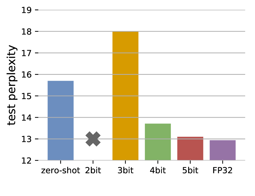
(a) Fine-tune WikiText2

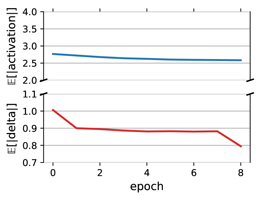
(b) Activation and delta

Figure 1: (a) Fine-tuning GPT2-1.5B with different activation precisions in communication; (b) Average absolute value of activations and their changes for GPT2-1.5B during training.

Table 1: Summary of technical results. AC-GC Evans and Aamodt (2021) and TinyScript Fu et al. (2020) assume that the returned gradient is unbiased, whereas AQ-SGD algorithm does not rely on such an assumption.

Algorithm	Assumptions	Conv. Rate
	on Quant. Grad.
SGD Bottou et al. (2018)	N/A	$\mathcal{O}(1/\sqrt{T})$
AC-GC Evans and Aamodt (2021)	Unbiased	$\mathcal{O}(1/\sqrt{T})$
TinyScript Fu et al. (2020)	Unbiased	$\mathcal{O}(1/\sqrt{T})$
AQ-SGD	N/A	$\mathcal{O}(1/\sqrt{T})$

Previous efforts on activation compression Han et al. (2016); Hubara et al. (2017); Jain et al. (2018); Chakrabarti and Moseley (2019); Chen et al. (2021a) illustrate, albeit mostly empirically, that large deep learning models can tolerate some compression errors on these activation values. However, when it comes to the underlying theoretical analysis, these efforts mostly make assumptions that do not apply to neural networks with non-linear activation functions — the only two recent efforts that claim theoretical convergence analysis Evans and Aamodt (2021); Fu et al. (2020) assume that an unbiased compression on activations leads to an unbiased error on the gradient. Not surprisingly, these algorithms lead to suboptimal quality under relatively aggressive compression, illustrated in Figure 1(a) — in many cases, using activation compression to fine-tune a model might be worse than zero-shot learning without any fine-tuning at all.

In this paper, we focus on the problem of activation compression for training language models over slow networks by asking the following:

• Q1. Can we design an algorithm for activation compression with rigorous theoretical guarantees on SGD convergence?

• Q2. Can such an algorithm be implemented efficiently without additional runtime overhead and outperform today’s activation compression algorithms without accuracy loss?

Our answers to both questions are Yes. (Contribution 1) We propose AQ-SGD, a novel algorithm for activation compression. The idea of AQ-SGD is simple — instead of directly compressing the activations, compress the change of activations for the same training example across epochs. Intuitively, we expect AQ-SGD to outperform simply compressing the activations because it enables an interesting “self-enforcing” dynamics: the more training stabilizes $\rightarrow$ the smaller the changes of the model across epochs $\rightarrow$ the smaller the changes of activations for the same training example across epochs $\rightarrow$ the smaller the compression error using the same #bits $\rightarrow$ training stabilizes more. (Contribution 2) The theoretical analysis of AQ-SGD is non-trivial since we have to analyze the above dynamics and connect it to SGD convergence, which is quite different from most of today’s results on gradient compression and error compensation. Under mild technical conditions and quantization functions with bounded error, we show that AQ-SGD converges with a rate of $O(1/\sqrt{T})$ for non-convex objectives, the same as vanilla SGD Bottou et al. (2018); Liu and Zhang (2021). To the best of our knowledge, AQ-SGD is the first activation compression algorithm with rigorous theoretical analysis that shows a convergence rate of $O(1/\sqrt{T})$ (without relying on assumptions of unbiased gradient). (Contribution 3) We then show that AQ-SGD can be optimized and implemented efficiently, without adding additional end-to-end runtime overhead over non-compression and other compression schemes (it does require us to utilize more memory and SSD for storage of activations). (Contribution 4) We then conduct extensive experiments on sequence classification and language modeling datasets using DeBERTa-1.5B and GPT2-1.5B models, respectively. We show that AQ-SGD can aggressively quantize activations to 2-4 bits without sacrificing convergence performance, where direct quantization of activations fails to converge; in slow networks, AQ-SGD achieves up to $4.3\times$ end-to-end speedup. (Contribution 5) Last but not least, we also show that AQ-SGD can be combined with state-of-the-art gradient compression algorithms to enable “end-to-end communication compression”: All data exchanges between machines, including model gradients, forward activations, and backward gradients are quantized into lower precision. This provides up to $4.9\times$ end-to-end speed-up, without sacrificing model quality.

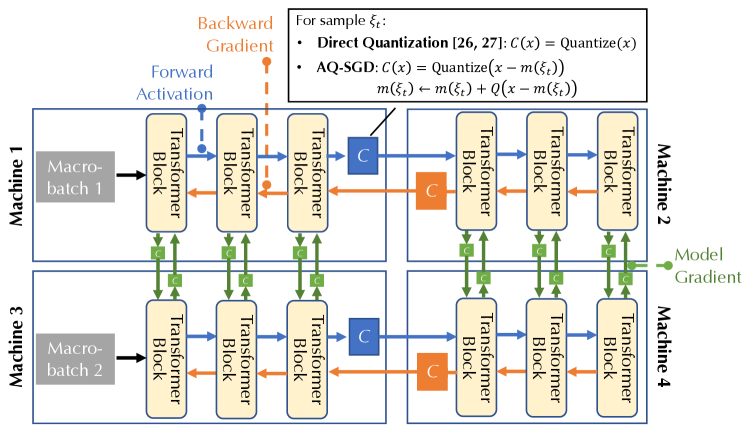
Figure 2: The communication pattern of training large language models with both data parallelism and pipeline model parallelism. $C$ denotes a compression module. The goal of this paper is to understand the design of $C$ for forward activation and backward gradient.

2 Overview and Problem Formulation

Training large language models over multiple devices is a challenging task. Because of the vast number of parameters of the model and data examples, state-of-the-art systems need to combine different forms of parallelism. Figure 2 illustrates an example in which such a model is distributed over four machines: (Pipeline Model Parallelism) The model is partitioned onto Machine 1 and Machine 2 (similarly, Machine 3 and Machine 4), each of which is holding a subset of layers. To compute the gradient over the model using backpropagation, these two machines need to communicate the activations during the forward pass and the gradient on activations during the backward pass. (Data Parallelism) Machine 1 and Machine 3 (similarly, Machine 2 and Machine 4) process the same set of layers for different macro-batches. In this case, each of them will hold a replica of the same model. After the gradient over their model parameters are ready, they need to communicate the model gradient, usually by taking an average Li et al. ; Sergeev and Del Balso (2018); Gan, Shaoduo and Lian, Xiangru and Wang, Rui and Chang, Jianbin and Liu, Chengjun and Shi, Hongmei and Zhang, Shengzhuo and Li, Xianghong and Sun, Tengxu and Jiang, Jiawei and others (2021).

Communication Compression for Forward Activations and Backward Gradients.

In slow networks, the communication among all machines often becomes the bottleneck Liu and Zhang (2021). To improve the speed of training, one can conduct lossy compression of the data before they are communicated, illustrated as the $C$ module in Figure 2. When the model fits into a single machine, there have been intensive efforts on compressing the model gradient Alistarh et al. (2016); Zhang et al. (2017); Bernstein et al. (2018); Wen et al. (2017). However, when it comes to pipeline model parallelism, such compression techniques are less studied. In this paper, we focus on designing efficient communication compression algorithms to compress both forward activations and backward gradients. As we will show later, both can be compressed significantly with AQ-SGD without hurting the model quality. We also show that it is possible to combine AQ-SGD with state-of-the-art gradient compression techniques to enable the end-to-end compression scheme illustrated in Figure 2.

Problem Formulation.

In this paper, we focus on the following technical problem. Note that, for the simplicity of notations, we present here the case where the model is partitioned onto $K=2$ machines. AQ-SGD works for cases with $K>2$: (1) in experiments, we consider $K=8$, i.e., a single model is partitioned onto 8 machines; (2) in the supplementary material we provide the theoretical analysis for $K>2$.

Given a distribution of samples $\mathcal{D}$, we consider the following optimization task:

$$\min_{x\in\mathbb{R}^{d}}\hskip 14.22636ptf(x):=\mathbb{E}_{\xi\sim\mathcal{D}}F(b(a(\xi,x^{(a)}),x^{(b)})),$$ (2.1)

where $F$ is a loss function, $a(-)$ and $b(-)$ correspond to two sets of layers of the model — $a(-)$ has model $x^{(a)}$ and $b(-)$ has model $x^{(b)}$. In Figure 2, Machine 1 would hold $x^{(a)}$ and Machine 2 would hold $x^{(b)}$. In the following, we call the machine that holds $x^{(a)}$ Machine $a$ and the machine that holds $x^{(b)}$ Machine $b$ . In the standard backpropagation algorithm, the communication between these two machines are as follows:

• Given a data sample $\xi$, Machine $a$ sends to Machine $b$ the forward activation: $a(\xi,x^{(a)})$

• Machine $b$ sends to Machine $a$ the backward gradient on $a(\xi,x^{(a)})$.

Difficulties in Direct Quantization.

A natural way at compressing forward activations is to send, instead of $a(\xi,x^{(a)})$, a quantized version $m(\xi,x^{(a)})=Q(a(\xi,x^{(a)}))$. This is the quantization scheme that state-of-the-art methods such as AC-GC Evans and Aamodt (2021) and TinyScript Fu et al. (2020) use. Both AC-GC Evans and Aamodt (2021) and TinyScript Fu et al. (2020) assume that gradient is unbiased when $m(\xi,x^{(a)})$ is an unbiased estimator of $a(\xi,x^{(a)})$. This enables their convergence rates of $\mathcal{O}(1/\sqrt{T})$. However, because of the non-linearity of $F$ and $b$ in a deep learning model with non-linear activation functions, an unbiased $m(\xi,x^{(a)})$ will lead to biases on the gradient. In Appendix, we will provide an example showing that such a gradient bias will hurt SGD convergence even for a very simple optimization problem. On the theory side, previous efforts on understanding gradient bias Ajalloeian and Stich (2020) have also shown that even bounded bias on gradient can impact the converges of SGD. As we will show later, empirically, this bias can indeed lead to suboptimal models under aggressive compression.

Notation.

Throughout the paper we use the following definitions:

• $f^{*}$ is the optimal value of $f$.

• $N$ is the number of samples.

• $x_{t}=(x_{t}^{(a)},x_{t}^{(b)})$ is the full model at iteration $t$.

• $\nabla f(\cdot)$ is the gradient of function $f$.

• $g_{\xi_{t}}(x_{t})=\nabla F(\xi_{t};x_{t})$ is the stochastic gradient.

• $Q(\cdot)$ is the quantization function used to compress activations.

• $m(\cdot)$ is the message exchanged between $a$ and $b$ in the feed forward path.

• $\|\cdot\|$ denotes the $L_{2}$-norm.

Algorithm 1 AQ-SGD Algorithm

1:  Initialize: $x_{0}$, learning rate $\gamma$, sub-network $a(-)$ weights $x^{(a)}$, sub-network $b(-)$ weights $x^{(b)}$, quantization function $Q$, array of previous messages $m$ initialized to 0

2:  for t = 1, …, T do

3:     Randomly sample $\xi_{t}$

4:     if $\xi_{t}$ not seen before then

5:        Set $m(\xi_{t})=a(\xi_{t},x_{t}^{(a)})$

6:     else

7:        Update $m(\xi_{t})\leftarrow m(\xi_{t})+Q\big{(}a(\xi_{t},x_{t}^{(a)})-m(\xi_{t})\big{)}$

8:     end if

9:     // Machine $a$ sends $Q\big{(}a(\xi_{t},x_{t}^{(a)})-m(\xi_{t})\big{)}$ to Machine $b$, which knows $m(\xi_{t})$ through a local version of $m$

10:     Update $x_{t+1}^{(b)}\leftarrow x_{t}^{(b)}-\gamma\cdot\nabla_{x^{(b)}}(f\circ b)|_{m}$

11:     // Machine $b$ sends $Q(\nabla_{a}(f\circ b)|_{m})$ to Machine $a$

12:     Update $x_{t+1}^{(a)}\leftarrow x_{t}^{(a)}-\gamma\cdot Q(\nabla_{a}(f\circ b)|_{m})\cdot\nabla_{x^{(a)}}a$

13:  end for

14:  Output: $x=(x_{T}^{(a)},x_{T}^{(b)})$

3 AQ-SGD: Theoretical Analysis and System Implementations

In this section we present the AQ-SGD, with the goal to mitigate the above mentioned difficulties that appear in direct quantization of the activation functions.

3.1 AQ-SGD Algorithm

Algorithm 1 illustrates the AQ-SGD algorithm. The idea behind Algorithm 1 is simple — instead of quantizing the activations directly, quantize the changes of activations for the same training example across epochs. As illustrated in Algorithm 1, for iteration $t$ and the data sample $\xi_{t}$, if it is the first time that $\xi_{t}$ is sampled, Machine $a$ communicates the full precision activations without any compression: $m(\xi_{t})=a(\xi_{t},x_{t}^{(a)})$ (Lines 4-5). Both machines will save $m(\xi_{t})$ in a local buffer. If $\xi_{t}$ has been sampled in previous iterations, Machine $a$ communicates a quantized version:

$$Q(a(\xi_{t},x_{t}^{(a)})-m(\xi_{t})),$$

where $m(\xi_{t})$ was the previous message, stored in the local buffer. Both machines then update this local buffer:

$$m(\xi_{t})\leftarrow m(\xi_{t})+Q(a(\xi_{t},x_{t}^{(a)})-m(\xi_{t})).$$

Machine $b$ then use $m(\xi_{t})$ as the forward activations, compute backward gradients, and communicate a quantized version of the backward gradient to Machine $a$ (Line 11). We use

$$\delta_{\xi}=a(\xi_{t},x_{t}^{(a)})-m(\xi_{t})$$

to denote the message error in sending the activations.

Update Rules. The above algorithm corresponds to the following update rules, at iteration $t$ with sample $\xi_{t}$:

$$x_{t+1}^{(a)} =x_{t}^{(a)}-\gamma\cdot Q(\nabla_{a}(f\circ b)|_{(m(\xi,x_{t}^{(a)}),x_{t}^{(b)})})\cdot\nabla_{x^{(a)}}a|_{x_{t}^{(a)}},$$

$$x_{t+1}^{(b)} =x_{t}^{(b)}-\gamma\cdot\nabla_{x^{(b)}}(f\circ b)|_{(m(\xi,x_{t}^{(a)}),x_{t}^{(b)})},$$

where $\gamma$ is the learning rate, $\nabla_{x^{(b)}}(f\circ b)|_{(m(\xi,x_{t}^{(a)}),x_{t}^{(b)})}$ is the gradient on $x^{(b)}$ using the quantized forward activations $(m(\xi,x_{t}^{(a)})$, and $Q(\nabla_{a}(f\circ b)|_{(m(\xi,x_{t}^{(a)}),x_{t}^{(b)})})$ is the quantized backward gradient.

Setting $x_{t}=(x_{t}^{(a)},x_{t}^{(b)})$, we can rephrase the update rule as

$$x_{t+1}=x_{t}-\gamma\cdot\left(g_{\xi}(x_{t})+\Delta_{\xi}(x_{t})\right),$$

where $g_{\xi}(x_{t})$ is the stochastic gradient and $\Delta_{\xi}(x_{t})$ is the gradient error introduced by communication compression. We have $\Delta_{\xi}=(\Delta_{\xi}^{(a)}+\Delta_{\xi}^{(Q)},\Delta_{\xi}^{(b)})$ given by:

$$\Delta_{\xi}^{(Q)}(x_{t}) =Q(\nabla_{a}(f\circ b)|_{(m(\xi,x_{t}^{(a)}),x_{t}^{(b)})})\cdot\nabla_{x^{(a)}}a|_{x_{t}^{(a)}}-\nabla_{a}(f\circ b)|_{(m(\xi,x_{t}^{(a)}),x_{t}^{(b)})}\cdot\nabla_{x^{(a)}}a|_{x_{t}^{(a)}},$$

$$\Delta_{\xi}^{(a)}(x_{t}) =\nabla_{a}(f\circ b)|_{(m(\xi,x_{t}^{(a)}),x_{t}^{(b)})}\cdot\nabla_{x^{(a)}}a|_{x_{t}^{(a)}}-\nabla_{a}(f\circ b\circ a)|_{(x_{t}^{(a)},x_{t}^{(b)})}$$

$$\Delta_{\xi}^{(b)}(x_{t}) =\nabla_{x^{(b)}}(f\circ b)|_{(m(\xi,x_{t}^{(a)}),x_{t}^{(b)})}-\nabla_{x^{(b)}}(f\circ b)|_{(a(\xi,x_{t}^{(a)}),x_{t}^{(b)})},$$

where $\Delta_{\xi}^{(Q)}(x_{t})$ is the error introduced by the gradient quantization in the backpropagation part, whilst $\Delta_{\xi}^{(a)}(x_{t})$ and $\Delta_{\xi}^{(b)}(x_{t})$ are the errors that the gradients of $a$ and $b$, respectively, inherit from the bias introduced in the forward pass.

3.2 Theoretical Analysis

We now prove the main theorem which states that, under some standard assumptions that are often used in the literature Bottou et al. (2018); Liu and Zhang (2021), the convergence rate of AQ-SGD algorithm is $O(1/\sqrt{T})$ for non-convex objectives, same as vanilla SGD.

Assumptions.

We make several assumptions on the networks and the quantization. It is important to note is that we put no restrictions on either the message error $\delta_{\xi}$, nor the gradient error $\Delta_{\xi}$.

• (A1: Lipschitz assumptions) We assume that $\nabla f$, $\nabla(f\circ b)$ and $a$ are $L_{f}$, $L_{f\circ b}$-, and $\ell_{a}$-Lipschitz, respectively, recalling that a function $g$ is $L_{g}$-Lipschitz if

  $$\|g(x)-g(y)\|\leq L_{g}\|x-y\|,\hskip 14.22636pt\forall x,\forall y.$$

  Furthermore, we assume that $a$ and $f\circ b$ have gradients bounded by $C_{a}$ and $C_{f\circ b}$, respectively, i.e. $\|\nabla a(x)\|\leq C_{a}$, and $\|\nabla(f\circ b)(x)\|\leq C_{f\circ b}$.

• (A2: SGD assumptions) We assume that the stochastic gradient $g_{\xi}$ is unbiased, i.e. $\mathbb{E}_{\xi}[g_{\xi}(x)]=\nabla f(x)$, for all $x$, and with bounded variance, i.e. $\mathbb{E}_{\xi}\|g_{\xi}(x)-\nabla f(x)\|^{2}\leq\sigma^{2}$, for all $x$.

Theorem 3.1.

Suppose that Assumptions A1, A2 hold, and consider an unbiased quantization function $Q(x)$ which satisfies that there exists $c_{Q}<\sqrt{1/2}$ such that $\mathbb{E}\|x-Q(x)\|\leq c_{Q}\|x\|$, for all $x$. Let $\gamma=\frac{1}{3(3L_{f}+C)\sqrt{T}}$ be the learning rate, where

$$C=\frac{4c_{Q}\ell_{a}(1+C_{a})L_{f\circ b}N}{\sqrt{1-2c_{Q}^{2}}}.$$

Then after performing $T$ updates one has

$$\frac{1}{T}\sum_{t\in[T]}\mathbb{E}\|\nabla f(x_{t})\|^{2}\lesssim\frac{(C+L_{f})(f(x_{1})-f^{*})}{\sqrt{T}}+\frac{\sigma^{2}+(c_{Q}C_{a}C_{f\circ b})^{2}}{\sqrt{T}}.$$ (3.1)

We present the full proof of Theorem 3.1 in Appendix A, whereas here we explain the main intuition. The usual starting point in examining convergence rates is to use the fact that $f$ has $L_{f}$-Lipschitz gradient. It is well known that this implies

$$\gamma\langle\nabla f(x_{t}),g_{\xi_{t}}(x_{t})\rangle+f(x_{t+1})-f(x_{t})\leq-\langle\nabla f(x_{t}),\Delta_{\xi_{t}}(x_{t})\rangle+\frac{\gamma^{2}L_{f}}{2}\|g_{\xi_{t}}(x_{t})+\Delta_{\xi_{t}}(x_{t})\|^{2}.$$

After taking the expectation over all $\xi_{t}$ and summing over all $t=1,\ldots,T$, we easily see that the key quantity to bound is $\sum_{t=1}^{T}\mathbb{E}\|\tilde{\Delta}_{\xi_{t}}(x_{t})\|^{2}$, where $\tilde{\Delta}_{\xi_{t}}(x_{t})=(\Delta_{\xi_{t}}^{(a)}(x_{t}),\Delta_{\xi_{t}}^{(b)}(x_{t}))$. On the other hand, the main object that we can control is the message error, $\delta_{\xi}$. Therefore, we first prove an auxiliary result which shows that $\|\tilde{\Delta}_{\xi_{t}}(x_{t})\|\leq(1+C_{a})\ell_{a}\|\delta_{\xi_{t}}(x_{t})\|$, for all $t$. The key arguments for bounding $\delta_{\xi_{t}}$ closely follow the self-improving loop described in the introduction, and can be summarized as follows. Since we are compressing the information in such a way that we compare with all the accumulated differences, this allows us to unwrap the changes which appeared since the last time that we observed the current sample, in an iterative way. However, since these are gradient updates, they are bounded by the learning rate — as long as we have a quantization method that keeps enough information about the signal, we can recursively build enough saving throughout the process. In particular, the more stability we have in the process, the smaller the changes of the model and the compression error gets, further strengthening the stability.

Tightness.

The bound is tight with respect to quantization — setting $c_{Q}=0$ (implying $C=0$), i.e. quantization does not incur any loss, recovers the original original SGD convergence (cf. Bottou et al. (2018); Liu and Zhang (2021)).

Regularization and other optimizers.

Assuming A1 and A2 for $f$, and under further assumptions on $b$ and $\nabla_{x^{(b)}}b$, one can prove that the $L_{2}$-regularized loss $\tilde{f}(x)=f(x)+\frac{\lambda}{2}\|x\|^{2}$, which results in weight decay, satisfies Assumptions A1 and A2 with slightly weaker constants. We note that a theoretical analysis for other regularization methods or optimizers such as Adam Kingma and Ba (2015), could be an independent study and represent an interesting line of future research.

3.3 System Implementations and Optimizations.

Additional storage and communication. AQ-SGD requires us to store, for each data example $\xi$, the quantized activation $m(\xi)$ in a local buffer in memory or SSD. For example, in GPT2-XL training, a simple calculation shows that we need an approximately extra 1TB storage. When using data parallelism, it reduces to 1TB / $\#$ parallel degree, but also incurs communication overhead if data is shuffled in every epoch. In addition, when the example $\xi$ is sampled again, $m(\xi)$ needs to be (1) loaded from this local buffer to the GPU, and (2) updated when a new value for $m(\xi)$ is ready.

Optimization. It is easy to implement and optimize the system such that this additional loading and updating step do not incur significant overhead on the end-to-end runtime. This is because of the fact that the GPU computation time for a forward pass is usually much longer than the data transfer time to load the activations — for GPT2-XL with 1.5 billion model parameters, a single forward pass on 6 layers require 44 ms, whereas loading $m(\xi)$ need 0.2 ms from memory and 12 ms from SSD. One can simply pre-fetch $m(\xi)$ right before the forward pass, and hide it within the forward pass of other data examples. Similarly, updating $m(\xi)$ can also be hidden in the backward computation. It is also simple to reduce the communication overhead by shuffling data only once or less frequently.

4 Evaluation

We demonstrate that AQ-SGD can significantly speed up fine-tuning large language models in slow networks. Specifically, we show: (1) on four standard benchmark tasks, AQ-SGD can tolerate aggressive quantization on the activations (2-4 bits) and backward gradients (4-8 bits), without hurting convergence and final loss, whereas direct quantization converges to a worse loss or even diverge, (2) in slow networks, AQ-SGD provide an end-to-end speed-up up to $4.3\times$, and (3) AQ-SGD can be combined with state-of-the-art gradient compression methods and achieve an end-to-end speed-up of up to $4.9\times$.

4.1 Experimental Setup

Datasets and Benchmarks. We consider both sequence classification and language modeling tasks with state-of-the-art foundation models. For sequence classification, we fine-tune a 1.5B parameter DeBERTa on two datasets: QNLI and CoLA. For language modeling, we fine-tune the GPT2 model with 1.5B parameters on two datasets: WikiText2 and arXiv abstracts. All datasets are publicly available and do not contain sensitive or offensive content. Detailed setup can be found in Appendix B.

Distributed Cluster. We conduct our experiments on AWS with 8-32 p3.2xlarge instances, each containing a V100 GPU. For a single pipeline, we partition a model onto 8 machines. When combined with data parallelism, we use 32 instances — data parallel degree is 4 and pipeline parallel degree is 8. By default, instances are interconnected with 10Gbps bandwidth. We simulate slow networks by controlling the communication bandwidth between instances using Linux traffic control.

Baselines. We compare with several strong baselines:

1. FP32: in which all communications are in 32 bit floating point without any compression.

2. DirectQ Evans and Aamodt (2021); Fu et al. (2020): in which activations and backward gradients are directly quantized.

We use a simple, uniform quantization scheme, which first normalizes a given vector into $[-1,1]$ and quantize each number into a $b$-bit integers by uniforming partitioning the range $[-1,1]$ into $2^{b}$ intervals Chakrabarti and Moseley (2019). Additional details of the configuration can be found in Appendix C.

Hyperparameter Tuning. We conduct careful tuning for all methods on all datasets. We perform grid search to choose learning rate from $\{$2.5e-6, 3e-6, 5e-6, 1e-5$\}$ and macro-batch size from $\{$32, 64, 96$\}$ for best model performance. We train all models using the Adam optimizer with weight decay.

4.2 Results

Convergence.

We first compare the convergence behavior of different methods. For all compression methods, we try various settings: fw$x$ bw$y$ means that we use $x$ bits for forward activation and $y$ bits for backward gradients. Figure 3 shows the convergence behavior for the sequence classification and language modeling tasks. FP32 converges fast since it does not introduce any compression errors. DirectQ, under aggressive quantization, can converge to a significantly worse model, or even diverge. This is not surprising, given the biases on model gradients that direct quantization introduced. On the other hand, AQ-SGD converges almost as fast as FP32 in terms of number of training steps.

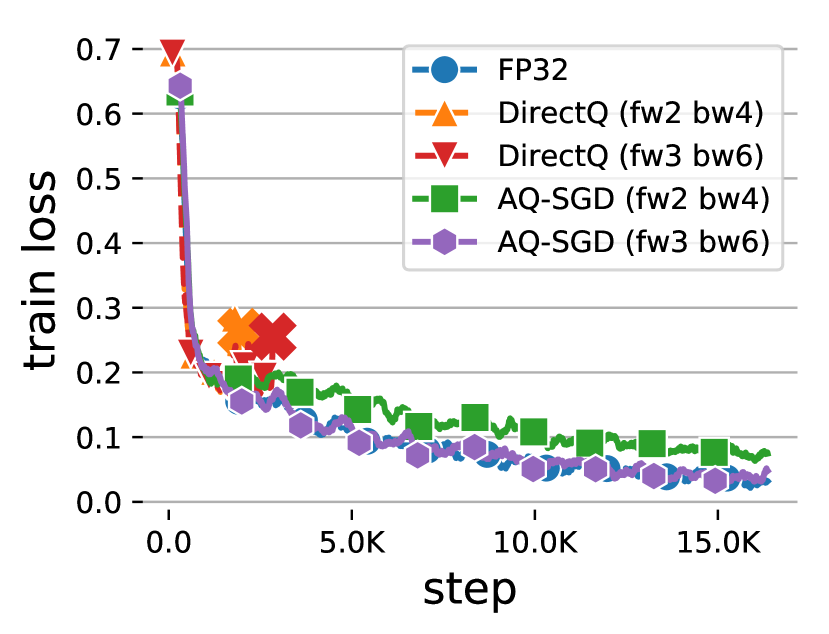
(a) QNLI, DeBERTa-1.5B

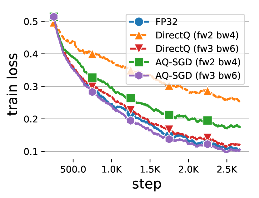
(b) CoLA, DeBERTa-1.5B

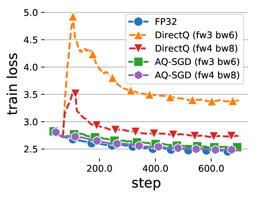
(c) WikiText2, GPT2-1.5B

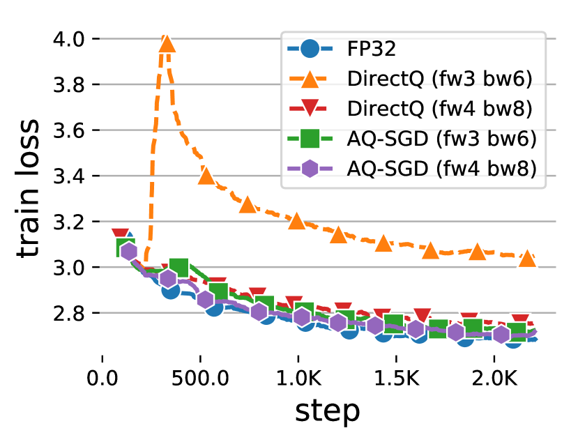
(d) arXiv, GPT2-1.5B

Figure 3: Convergence (loss vs. # steps) of different approaches. $\boldsymbol{\times}$ represents divergence.

End-to-End Runtime.

We show the end-to-end runtime of different methods under slow networks. As illustrated in Figure 4, AQ-SGD achieves a 4.3$\times$ end-to-end speed-up comparing with that of FP32 (in terms of time to the same loss), illustrating the importance of communication compression in slow networks. Table 3 shows the training throughput and Table 3 shows the breakdown of our algorithm. We note that computation and communication can overlap, so the end-to-end time depends on the larger one of the two. Another interesting observation is that when the network is $100\times$ slower (from 10Gbps to 100Mbps), the training is only about $1.18\times$ slower! This is exciting — if AQ-SGD were to be deployed in a in real-world geo-distributed decentralized networks, the training throughput would be almost as fast as the performance inside a data center!

Moreover, AQ-SGD does not introduce significant runtime overhead over direct quantization. From Table 3, we see that AQ-SGD is essentially as efficient as direct quantization compression in throughput.

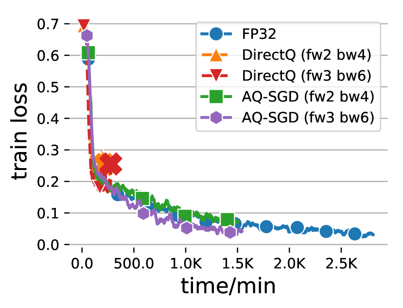
(a) QNLI, 500Mbps

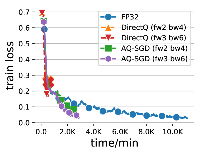
(b) QNLI, 100Mbps

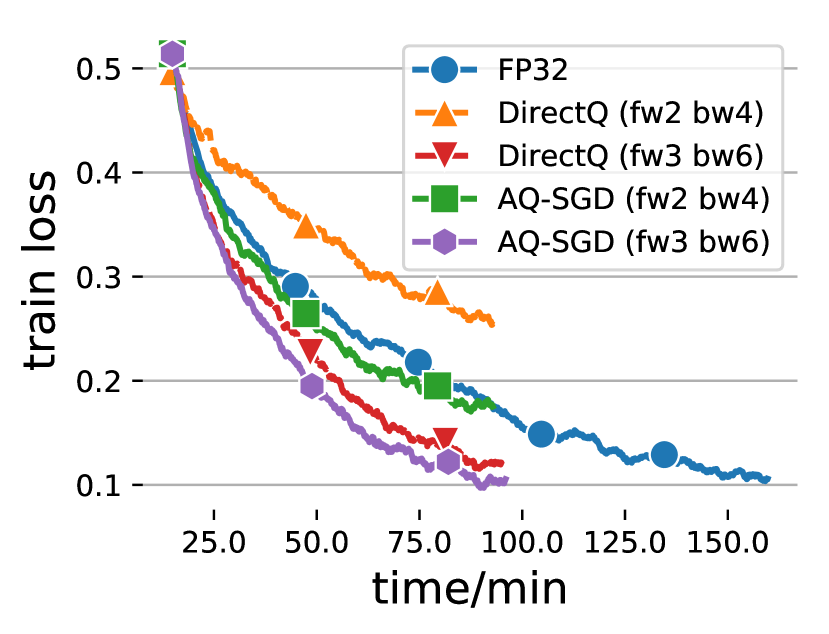
(c) CoLA, 500Mbps

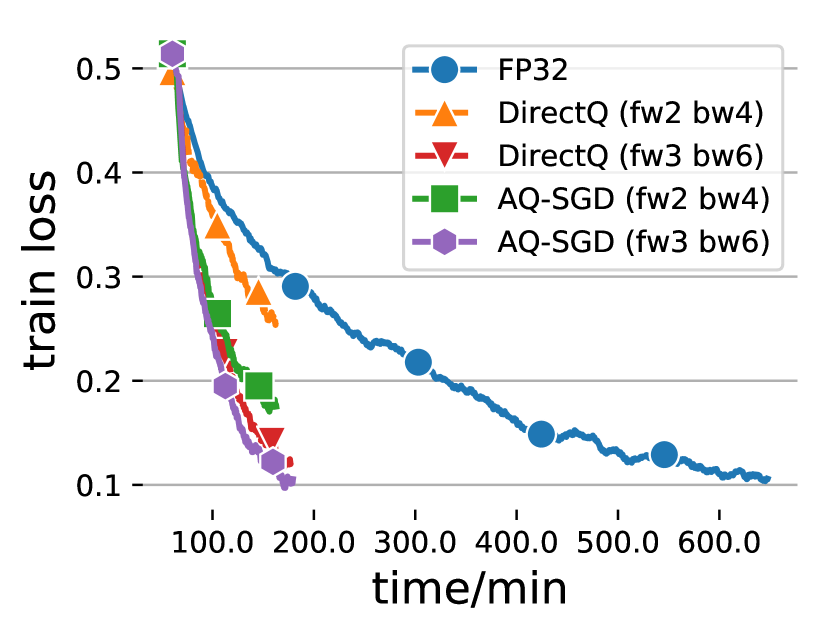
(d) CoLA, 100Mbps

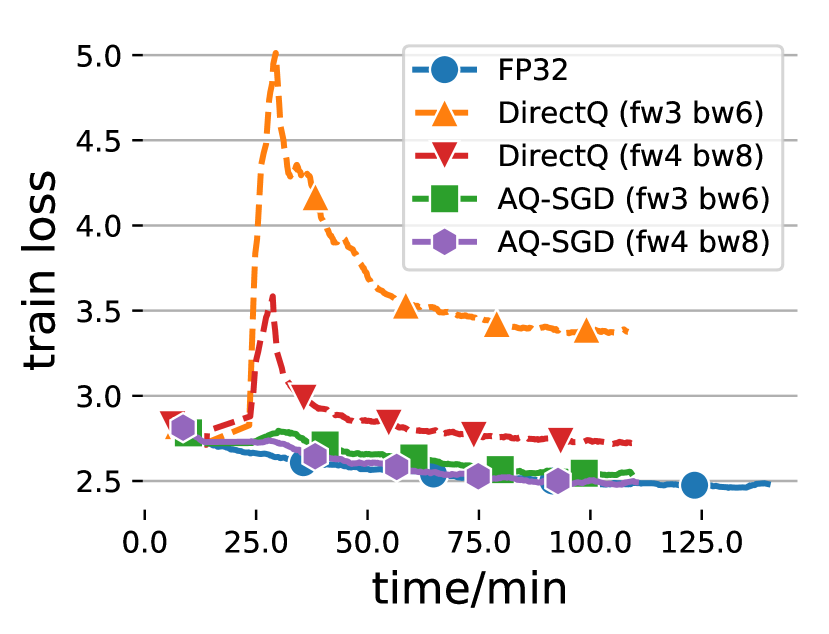
(e) WikiText2, 500Mbps

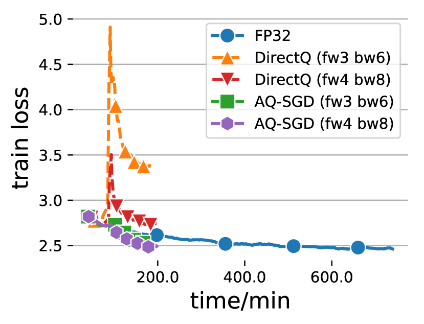
(f) WikiText2, 100Mbps

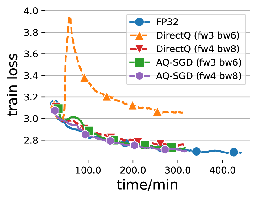
(g) arXiv, 500Mbps

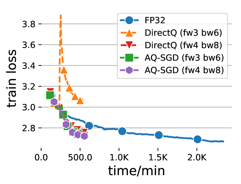
(h) arXiv, 100Mbps

Figure 4: End-to-end training performance over different networks. $\boldsymbol{\times}$ represents divergence.

Table 2: Training Throughput of GPT2-1.5B. Others are similar and shown in Appendix.

Network Bandwidth	FP32	DirectQ fw3 bw6 / fw4 bw8	AQ-SGD fw3 bw6 / fw4 bw8
10 Gbps	3.8	4.0    /    4.1	4.0    /    4.0
1 Gbps	3.2	4.0    /    4.0	4.0    /    3.9
500 Mbps	2.7	3.9    /    3.9	3.9    /    3.9
300 Mbps	1.8	3.9    /    3.8	3.8    /    3.8
100 Mbps	0.5	3.5    /    3.0	3.4    /    3.0

Table 3: Breakdown of AQ-SGD (fw4 bw8) on GPT2-1.5B. We show the computation and communication time of each micro batch.

Network Bandwidth	Forward pass		Backward pass
	comp.	comm.	comp.	comm.
500 Mbps	45 ms	13 ms	135 ms	25 ms
300 Mbps	45 ms	21 ms	135 ms	42 ms
200 Mbps	45 ms	31 ms	135 ms	63 ms
100 Mbps	45 ms	63 ms	135 ms	125 ms

4.3 End-to-end Communication Compression: AQ-SGD + QuantizedAdam

AQ-SGD can also be combined with existing methods on gradient compression. This allows us to compress all communications during training. We combine AQ-SGD with QuantizedAdam Tang et al. (2021), an error compensation-based gradient compression algorithm for data parallel training.

We quantize the forward activations with 3 bits, the backward gradient with 6 bits, and model gradient with 4 bits. Figure 5 illustrates the convergence and the training throughput under different network configuration. We see that AQ-SGD converges well when combined with QuantizedAdam (Figure 5(a, b)). On the other hand, DirectQ, when combined with gradient compression, converges to a much worse model. In terms of training throughput, with both activation and gradient compression, we can achieve up to 8.5$\times$ throughput improvement compared to the no-compression baseline (Figure 5(c)). We also see that both activation and gradient compression are important in terms of improving end-to-end training throughput — as illustrated in Figure 5(c), disabling any of them will lead to a much lower training throughput.

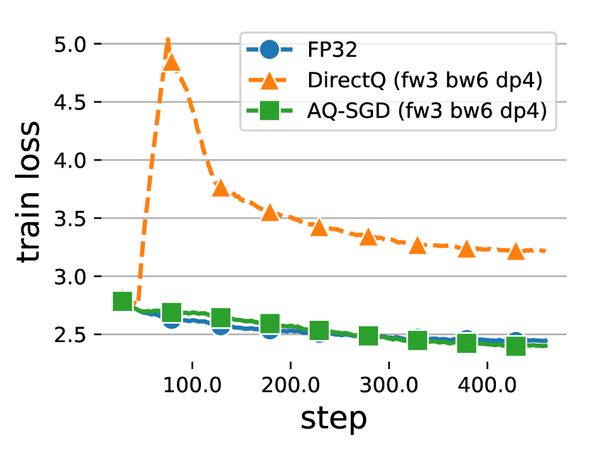
(a) WikiText2, GPT2-1.5B

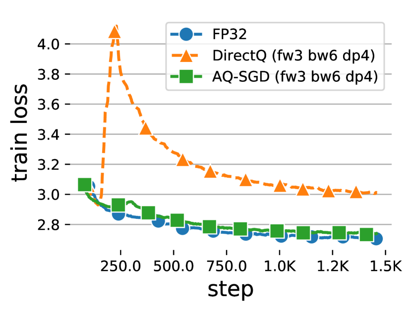
(b) arXiv, GPT2-1.5B

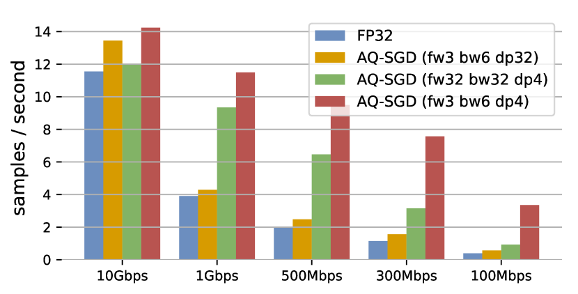
(c) Training Throughput

Figure 5: Convergence and Throughput of AQ-SGD combined with gradient compression.

5 Related Work

Distributed training of foundation models. Modern distributed training of deep neural networks goes beyond data parallelism Shoeybi et al. (2019); Huang et al. (2019); Yang et al. (2021) due to the advance of the large-scale foundation models Bommasani et al. (2021), such as BERT Devlin et al. (2018), GPT-3 Brown et al. (2020), and CLIPRadford et al. (2021). Popular systems to support foundation model training include Megatron Shoeybi et al. (2019), Deepspeed Rasley et al. (2020), and Fairscale Baines et al. (2021). To scale out the training of large-scale models, pipeline parallelism (e.g., GpipeHuang et al. (2019), PipedreamNarayanan et al. (2019, 2021)) is a popular option, where the model is partitioned into multiple stages, different stages are allocated on different GPUs and the exchange of activations and gradients on activations goes through network communication.

Communication compression of distributed learning. Communication compression is an effective system relaxation for distributed training, especially in data parallelism Tang et al. (2021); Chen et al. (2020); Xie et al. (2020); Faghri et al. (2020); Li et al. (2020); Rothchild et al. (2020); Safaryan and Richtárik (2021); Gorbunov et al. (2021); Safaryan et al. (2021); Qian et al. (2021); M Abdelmoniem et al. (2021); Wang et al. (2021). Popular techniques include quantization Alistarh et al. (2016); Zhang et al. (2017); Bernstein et al. (2018); Wen et al. (2017), sparsification Wangni et al. (2018); Alistarh et al. (2018); Wang et al. (2018, 2017), sketching Jiang et al. (2018); Ivkin et al. (2019) and error compensation Tang et al. (2019a). Recently, TinyScript Fu et al. (2020) proposes to compress activations and gradients simultaneously.

Sparse Learning for activation compression. Sparse learning Fu et al. (2020); Mocanu et al. (2018); Raihan and Aamodt (2020); Chen et al. (2021b); Dettmers and Zettlemoyer (2019); Mostafa and Wang (2019); Junjie et al. (2019); Hoefler et al. (2021); Liu et al. (2021a) has become increasingly popular for training neural networks, as it can significantly reduce the use of computation and memory while preserving the generalization of such models. In particular, activation compression methods Han et al. (2016); Hubara et al. (2017); Jain et al. (2018); Chakrabarti and Moseley (2019); Chen et al. (2021a); Evans and Aamodt (2021) are proposed to reduce the memory footprint by adopting lossless Choukse et al. (2020); Rhu et al. (2018); Lascorz et al. (2019) and lossy Jin et al. (2021); Evans and Aamodt (2021); Evans et al. (2020) compression techniques in the training of various deep neural networks (e.g., CNNMostafa and Wang (2019); Georgiadis (2019); Gudovskiy et al. (2018), GNNLiu et al. (2021b)). These approaches usually compute the activation with full precision in forward propagation, adopt the compression method over the activation, and store the compressed version in DRAM for later use in backward propagation. Thus, compression does not introduce any error in forward propagation in contrast to the scenario of communicating compressed activation in the distributed setting.

Delta-based compression. Delta-based compression Pekhimenko et al. (2012) is a classic solution to various system problems. Recent research has also used the property of spatial proximity within activation in neural network training based on empirical observations Awad et al. (2021); Bersatti et al. (2020); Evans et al. (2020). However, to our knowledge, no attempt has been made to consider the proximity of activation through training epochs to enable efficient compression with theoretical guarantee.

6 Conclusion

In this paper, we discuss how to adopt communication compression for activations in distributed learning. We proposed AQ-SGD, a novel activation compression algorithm for communication-efficient pipeline parallelism training over slow networks. AQ-SGD achieves $O(1/\sqrt{T})$ convergence rate for non-convex optimization without making assumptions on gradient unbiasedness. Our empirical study suggests that AQ-SGD can achieve up to $4.3\times$ speedup for pipeline parallelism. When combined with gradient compression in data parallelism, the end-to-end speed-up can be up to $4.9\times$.

Appendix A Proof of the Main Theorem

In this section we prove Theorem 3.1. The main idea comes from the “self-enforcing” dynamics described in the introduction of this work: the more training stabilizes $\rightarrow$ the smaller the changes of the model across epochs $\rightarrow$ the smaller the changes of activations for the same training example across epochs $\rightarrow$ the smaller the compression error using the same #bits $\rightarrow$ training stabilizes more.

We start by providing two auxiliary results. The first one connects the message error and the gradient error.

Lemma A.1.

For every sample $\xi$, one has

$$\|\Delta_{\xi}^{(Q)}(x)\|\leq c_{Q}C_{a}C_{f\circ b},$$

and

$$\|\tilde{\Delta}_{\xi}(x)\|\leq(1+C_{a})L_{f\circ b}\|\delta_{\xi}(x)\|,$$

where $\tilde{\Delta}_{\xi}(x)=(\Delta_{\xi}^{(a)}(x),\Delta_{\xi}^{(b)})$.

Proof:   Note that

$$\|\Delta_{\xi}^{(Q)}(x_{t})\| =\|\nabla_{x}a(\xi,x)_{x=x_{t}^{(a)}}\|\cdot\|Q(\nabla_{x}(f\circ b)(x,x_{t}^{(b)})_{x=m(\xi,x_{t}^{(a)})})-\nabla_{x}(f\circ b)(x,x_{t}^{(b)})_{x=m(\xi,x_{t}^{(a)})}\|$$

$$\leq C_{a}c_{Q}\|\nabla_{x}(f\circ b)(x,x_{t}^{(b)})_{x=m(\xi,x_{t}^{(a)})}\|\leq c_{Q}C_{a}C_{f\circ b},$$

$$\|\Delta_{\xi}^{(a)}(x_{t})\| =\|\nabla_{x}a(\xi,x)_{x=x_{t}^{(a)}}\|\cdot\|\nabla_{x}(f\circ b)(x,x_{t}^{(b)})_{x=m(\xi,x_{t}^{(a)})}-\nabla_{x}(f\circ b)(x,x_{t}^{(b)})_{x=a(\xi,x_{t}^{(a)})}\|$$

$$\leq C_{a}L_{f\circ b}\|(m(\xi,x_{t}^{(a)}),x_{t}^{(b)})-(a(\xi,x_{t}^{(a)}),x_{t}^{(b)})\|=C_{a}L_{f\circ b}\|\delta_{\xi}(x_{t})\|,$$

$$\|\Delta_{\xi}^{(b)}(x_{t})\| =\|\nabla_{y}(f\circ b)(m(\xi,x_{t}^{(a)}),y)_{y=x_{t}^{(b)}}-\nabla_{y}(f\circ b)(a(\xi,x_{t}^{(a)}),y)_{y=x_{t}^{(b)}}\|$$

$$\leq L_{f\circ b}\|(m(\xi,x_{t}^{(a)}),x_{t}^{(b)})-(a(\xi,x_{t}^{(a)}),x_{t}^{(b)})\|=L_{f\circ b}\|\delta_{\xi}(x_{t})\|,$$

which together with $\|\tilde{\Delta}_{\xi}(x_{t})\|=\|\Delta_{\xi}^{(a)}(x_{t})\|+\|\Delta_{\xi}^{(b)}(x_{t})\|$ yields the claim. ∎

We now prove that the message error can be efficiently bounded by the true gradient.

Lemma A.2.

For $C^{\prime}=\frac{18c_{Q}^{2}l_{a}^{2}N^{2}}{1-2c_{Q}^{2}}$, one has

$$\frac{1}{T}\sum_{t\in[T]}\mathbb{E}\|\delta_{\xi_{t}}(x_{t})\|^{2}\leq C^{\prime}\gamma^{2}\cdot\left(\frac{1}{T}\sum_{t\in[T]}\mathbb{E}\|\nabla f(x_{t})\|^{2}+\sigma^{2}+(c_{Q}C_{a}C_{f\circ b})^{2}\right).$$

Proof:   Let $\xi$ be a fixed sample. To simplify the exposition, we abuse the notation slightly by $a(x)=a(\xi,x)$, $m(x)=m(\xi,x)$. Let $T(\xi)$ be the number of realizations of $\xi$ before time $T$. Using the definition of $\delta_{\xi}$ (recalling that $\delta_{\xi}(x_{t_{1}(\xi)})=0$, since in the first iteration we send the correct signal), we have

$$\sum_{k=1}^{T(\xi)}\|\delta_{\xi}(x_{t_{k}(\xi)})\|^{2} =\sum_{k=2}^{T(\xi)}\|a(x_{t_{k}(\xi)})-m(x_{t_{k}(\xi)})\|^{2}$$

$$=\sum_{k=2}^{T(\xi)}\|a(x_{t_{k}(\xi)})-m(x_{t_{k-1}(\xi)})-Q(a(x_{t_{k}(\xi)})-m(x_{t_{k-1}(\xi)}))\|^{2}$$

$$\{\|x-Q(x)\|\leq c_{Q}\|x\|\}\hskip 28.45274pt \leq c_{Q}^{2}\sum_{k=2}^{T(\xi)}\|a(x_{t_{k}(\xi)})-a(x_{t_{k-1}(\xi)})+\delta_{\xi}(x_{t_{k-1}(\xi)})\|^{2}$$

$$\{(\alpha+\beta)^{2}\leq 2\alpha^{2}+2\beta^{2}\}\hskip 28.45274pt \leq 2c_{Q}^{2}\sum_{k=2}^{T(\xi)}\|a(x_{t_{k}(\xi)})-a(x_{t_{k-1}(\xi)})\|^{2}+2c_{Q}^{2}\sum_{k=2}^{T(\xi)}\|\delta_{\xi}(x_{t_{k-1}(\xi)})\|^{2}$$

$$\{a\text{ is }\ell_{a}\text{-Lipschitz }\}\hskip 28.45274pt \leq 2c_{Q}^{2}\ell_{a}^{2}\sum_{k=2}^{T(\xi)}\|x_{t_{k}(\xi)}-x_{t_{k-1}(\xi)}\|^{2}+2c_{Q}^{2}\sum_{k=2}^{T(\xi)}\|\delta_{\xi}(x_{t_{k-1}(\xi)})\|^{2}.$$

Transferring the $\delta_{\xi}$ part to the LHS, and noting that between every two realizations of $\xi$ at times $t_{k-1}(\xi)$ and $t_{k}(\xi)$, we can follow updates for $t=t_{k-1}(\xi),\ldots,t_{k}(\xi)-1$, we get

$$(1-2c_{Q}^{2})\sum_{k=1}^{T(\xi)}\|\delta_{\xi}(x_{t_{k}(\xi)})\|^{2} \leq\gamma^{2}\cdot(2c_{Q}^{2}\ell_{a}^{2})\sum_{k=1}^{T(\xi)}\left\|\sum_{t=t_{k-1}(\xi)}^{t_{k}(\xi)-1}\left(g_{\xi_{t}}(x_{t})+\Delta_{\xi_{t}}(x_{t})\right)\right\|^{2}$$

$$\{\text{Cauchy-Schwarz}\}\hskip 14.22636pt \leq\gamma^{2}\cdot(2c_{Q}^{2}\ell_{a}^{2})\sum_{k=1}^{T(\xi)}(t_{k}(\xi)-t_{k-1}(\xi))\sum_{t=t_{k-1}(\xi)}^{t_{k}(\xi)-1}\left\|g_{\xi_{t}}(x_{t})+\Delta_{\xi_{t}}(x_{t})\right\|^{2}$$

$$=\gamma^{2}\cdot(2c_{Q}^{2}\ell_{a}^{2})\sum_{t\in[T]}\omega_{\xi}(t)\cdot\|g_{\xi_{t}}(x_{t})+\Delta_{\xi_{t}}(x_{t})\|^{2},$$

where $\omega\colon[T]\rightarrow\{0,1,\ldots\}$ is defined by $\omega_{\xi}(t)=t_{k}(\xi)-t_{k-1}(\xi)$, if $t\in[t_{k-1}(\xi),t_{k}(\xi)-1]$, and $\omega_{\xi}(t)=0$, if $t>t_{T(\xi)}(\xi)$. We note that for two different samples $\xi$ and $\xi^{\prime}$, the sums on the LHS are disjoint. Therefore, summing over all samples $\xi$ and taking the expectation over $\xi$ and all $\xi_{t}$ yields

$$(1-2c_{Q}^{2})\cdot\frac{1}{T}\sum_{t\in[T]}\mathbb{E}\|\delta_{\xi_{t}}(x_{t})\|^{2} \leq\gamma^{2}\cdot(2c_{Q}^{2}\ell_{a}^{2})\cdot\frac{1}{T}\sum_{t\in[T]}\mathbb{E}\|g_{\xi_{t}}(x_{t})+\Delta_{\xi_{t}}(x_{t})\|^{2}\cdot N\cdot\mathbb{E}[\omega_{\xi}(t)]$$

$$\leq\gamma^{2}\cdot(2c_{Q}^{2}\ell_{a}^{2}N^{2})\cdot\frac{1}{T}\sum_{t\in[T]}\mathbb{E}\|g_{\xi_{t}}(x_{t})+\Delta_{\xi_{t}}(x_{t})\|^{2},$$

since $\mathbb{E}[\omega_{\xi}(t)]\leq N$. Applying $\|g_{\xi_{t}}(x_{t})+\Delta_{\xi_{t}}(x_{t})\|^{2}\leq 3\|g_{\xi_{t}}(x_{t})\|^{2}+3\|\Delta_{\xi_{t}}^{(Q)}(x_{t})\|^{2}+3\|\tilde{\Delta}_{\xi_{t}}(x_{t})\|^{2}$, bounded variance $\mathbb{E}\|g_{\xi}(x)-\nabla f(x)\|^{2}\leq\sigma^{2}$, and Lemma A.1, we get

$$\left(1-2c_{Q}^{2}-\gamma^{2}\cdot 6c_{Q}^{2}\ell_{a}^{2}N^{2}(1+C_{a})^{2}L_{f\circ b}^{2}\right)\cdot\frac{1}{T}\sum_{t\in[T]}\mathbb{E}\|\delta_{\xi_{t}}(x_{t})\|^{2}$$

$$\hskip 85.35826pt\leq\gamma^{2}\cdot(6c_{Q}^{2}\ell_{a}^{2}N^{2})\left(2\sigma^{2}+2\cdot\frac{1}{T}\sum_{t\in[T]}\mathbb{E}\|\nabla f(x_{t})\|^{2}+(c_{Q}C_{a}C_{f\circ b})^{2}\right),$$

which implies

$$\left(1-2c_{Q}^{2}-\gamma^{2}\cdot\frac{3}{8}\cdot C^{2}\cdot(1-2c_{Q}^{2})\right)\cdot\frac{1}{T}\sum_{t\in[T]}\mathbb{E}\|\delta_{\xi_{t}}(x_{t})\|^{2}$$

$$\hskip 85.35826pt\leq\gamma^{2}\cdot(12c_{Q}^{2}\ell_{a}^{2}N^{2})\left(\sigma^{2}+\frac{1}{T}\sum_{t\in[T]}\mathbb{E}\|\nabla f(x_{t})\|^{2}+(c_{Q}C_{a}C_{f\circ b})^{2}\right),$$

Recalling the definitions of $C$ and $\gamma$, and the fact that $\gamma\cdot C<\frac{1}{3}$, we can simplify the LHS to get

$$\left(1-2c_{Q}^{2}\right)\cdot\frac{1}{T}\sum_{t\in[T]}\mathbb{E}\|\delta_{\xi_{t}}(x_{t})\|^{2}\leq\gamma^{2}\cdot(12\cdot\frac{24}{23}\cdot c_{Q}^{2}\ell_{a}^{2}N^{2})\left(\sigma^{2}+\frac{1}{T}\sum_{t\in[T]}\mathbb{E}\|\nabla f_{\xi_{t}}(x_{t})\|^{2}+(c_{Q}C_{a}C_{f\circ b})^{2}\right),$$

yielding the claim. ∎

We are ready to prove the main result, with a learning rate of

$$\gamma=\frac{1}{3(3L_{f}+C)\sqrt{T}}.$$

Proof of Theorem 3.1:   Since $f$ has $L_{f}$-Lipschitz gradient, we know that

$$f(x_{t+1})-f(x_{t}) \leq-\gamma\cdot\langle\nabla f(x_{t}),g_{\xi_{t}}(x_{t})+\Delta_{\xi_{t}}(x_{t})\rangle+\frac{\gamma^{2}L_{f}}{2}\|g_{\xi_{t}}(x_{t})+\Delta_{\xi_{t}}(x_{t})\|^{2}.$$

Since the quantization is unbiased, implying $\mathbb{E}_{Q}[\Delta_{\xi}^{(Q)}(x)]=0$, taking the expectation with respect to the quantization yields

$$\mathbb{E}_{Q}[f(x_{t+1})]-\mathbb{E}_{Q}[f(x_{t})]$$

$$\hskip 28.45274pt\leq-\gamma\mathbb{E}_{Q}\langle\nabla f(x_{t}),g_{\xi_{t}}(x_{t})+\tilde{\Delta}_{\xi_{t}}(x_{t})\rangle+\frac{3\gamma^{2}L_{f}}{2}\left(\|g_{\xi_{t}}(x_{t})\|^{2}+\|\tilde{\Delta}_{\xi_{t}}(x_{t})\|^{2}+\mathbb{E}_{Q}\|\Delta_{\xi_{t}}^{(Q)}\|^{2}\right),$$

where $\tilde{\Delta}_{\xi_{t}}(x_{t})=(\Delta_{\xi_{t}}^{(a)},\Delta_{\xi_{t}}^{(b)})$, and we used $(\alpha+\beta+\rho)^{2}\leq 3\alpha^{2}+3\beta^{2}+3\rho^{2}$.

Taking the expectation over $\xi_{t}$ (simplifying the notation of $\mathbb{E}_{Q}\mathbb{E}_{\xi}$ to simply $\mathbb{E}$), and recalling that $\mathbb{E}[g_{\xi_{t}}(x_{t})]=\nabla f(x_{t})$, we can bound the first two terms of the RHS by

$$-\gamma\mathbb{E}\langle\nabla f(x_{t}),g_{\xi_{t}}(x_{t})+\tilde{\Delta}_{\xi_{t}}(x_{t})\rangle+\frac{3}{4}\gamma^{2}L_{f}\mathbb{E}\|g_{\xi_{t}}(x_{t})+\tilde{\Delta}_{\xi_{t}}(x_{t})\|^{2}$$

$$\leq-\frac{\gamma}{2}\mathbb{E}\|\nabla f(x_{t})\|^{2}+\frac{\gamma}{2}\mathbb{E}\|\tilde{\Delta}_{\xi_{t}}(x_{t})\|^{2}+\frac{3}{2}\gamma^{2}L_{f}\mathbb{E}\left(\|g_{\xi_{t}}(x_{t})\|^{2}+\|\tilde{\Delta}_{\xi_{t}}(x_{t})\|^{2}\right)\hskip 14.22636pt\{\alpha\cdot\beta\leq\frac{1}{2}(\alpha^{2}+\beta^{2})\}$$

$$\leq\left(-\frac{\gamma}{2}+3\gamma^{2}L_{f}\right)\mathbb{E}\|\nabla f(x_{t})\|^{2}+\left(\frac{\gamma}{2}+\frac{3}{2}\gamma^{2}L_{f}\right)\mathbb{E}\|\tilde{\Delta}_{\xi_{t}}(x_{t})\|^{2}+3\gamma^{2}L_{f}\sigma^{2}\hskip 5.69054pt\{\mathbb{E}\|g_{\xi_{t}}-\nabla f\|^{2}\leq\sigma^{2}\}$$

$$\leq\left(-\frac{\gamma}{2}+3\gamma^{2}L_{f}\right)\mathbb{E}\|\nabla f(x_{t})\|^{2}$$

$$\hskip 56.9055pt+\left(\frac{\gamma}{2}+\frac{3}{2}\gamma^{2}L_{f}\right)(1+C_{a})^{2}L_{f\circ b}^{2}\mathbb{E}\|\delta_{\xi_{t}}(x_{t})\|^{2}+3\gamma^{2}L_{f}\sigma^{2}.\hskip 14.22636pt\{\text{Lemma~{}\ref{lemAuxTwo}}\}$$

Reorganizing the terms, summing over all $t\in[T]$ and dividing by $T$ yields

$$\gamma\cdot\left(\frac{1}{2}-3\gamma L_{f}\right)\cdot\frac{1}{T}\sum_{t\in[T]}\mathbb{E}\|\nabla f(x_{t})\|^{2} \leq\frac{f(x_{1})-\mathbb{E}[f(x_{T+1})]}{T}+\gamma\cdot C^{\prime\prime}\cdot\frac{1}{T}\sum_{t\in[T]}\mathbb{E}\|\delta_{\xi_{t}}(x_{t})\|^{2}$$

$$\hskip 85.35826pt+\gamma^{2}L_{f}(3\sigma^{2}+\frac{3}{2}\cdot(c_{Q}C_{a}C_{f\circ b})^{2}),$$

where

$$C^{\prime\prime}=\left(\frac{1}{2}+\frac{3}{2}\gamma L_{f}\right)(1+C_{a})^{2}L_{f\circ b}^{2}<(1+C_{a})^{2}L_{f\circ b}^{2},$$ (A.1)

by the definition of $\gamma$. Applying Lemma A.2 and regrouping the terms now yields

$$\gamma\cdot\left(\frac{1}{2}-3\gamma L_{f}-\gamma^{2}\cdot C^{\prime}C^{\prime\prime}\right)\cdot\frac{1}{T}\sum_{t\in[T]}\|\nabla f(x_{t})\|^{2}$$

$$\hskip 56.9055pt\leq\frac{f(x_{1})-\mathbb{E}[f(x_{T+1})]}{T}+\gamma^{2}\left(\gamma\cdot C^{\prime}C^{\prime\prime}+3L_{f}\right)\cdot(\sigma^{2}+(c_{Q}C_{a}C_{f\circ b})^{2}).$$

Noting that $C^{\prime}C^{\prime\prime}<C^{2}$ and recalling that $\gamma C<1/3$ and $\gamma L_{f}<1/9$, we get

$$\gamma\cdot\left(\frac{1}{2}-\gamma(3L_{f}+C)\right)\cdot\frac{1}{T}\sum_{t\in[T]}\|\nabla f_{\xi_{t}}(x_{t})\|^{2}$$

$$\hskip 56.9055pt\leq\frac{f(x_{1})-\mathbb{E}[f(x_{T+1})]}{T}+\gamma^{2}\left(3L_{f}+C\right)\cdot(\sigma^{2}+(c_{Q}C_{a}C_{f\circ b})^{2}).$$

Since $\gamma\cdot(3L_{f}+C)=\frac{1}{3\sqrt{T}}\leq\frac{1}{3}$, the LHS coefficent is at least $\gamma/6$, so dividing by $\gamma/6$ now yields the claim by substituting $\gamma$ with $\frac{1}{3(3L_{f}+C)\sqrt{T}}$. ∎

A.1 Theoretical analysis when $K>2$

In this section we sketch how one can generalize the already provided theoretical analysis for the $K=2$ case.

Instead of Machines $a$ and $b$, we now suppose that we have a stack $a_{1}$, …, $a_{K}$ of $K$ Machines such that every pair $a_{i},a_{i+1}$ communicates a compressed message, denoted by $m_{i}$. We simplify the notation of the complete model by $x=(x^{(1)},\ldots,x^{(K)})$, and, for a sample $\xi$, further denote

$$\overline{a}^{(i)}(\xi,x_{t}) =a_{i}(a_{i-1}(\ldots(a_{1}(\xi,x_{t}^{(1)}),x_{t}^{(2)}),\ldots x_{t}^{(i)})),$$

$$\overline{m}^{(i)}(\xi,x_{t}) =m_{i}(m_{i-1}(\ldots(m_{1}(\xi,x_{t}^{(1)}),x_{t}^{(2)}),\ldots x_{t}^{(i)})),$$

for $i\in[K]$. As in Algorithm 1, for iteration $t$ and the data sample $\xi_{t}$, if it is the first time that $\xi_{t}$ is sampled, Machine $a_{i}$ communicates to Machine $a_{i+1}$ the full precision activations without any compression: $m_{i}(\xi_{t})=\overline{a}^{(i)}(\xi_{t},x_{t})$. If $\xi_{t}$ has been sampled in previous iterations, Machine $a_{i}$ communicates a compressed version:

$$Q(a_{i}(\overline{m}^{(i-1)}(\xi_{t}),x_{t}^{(i)})-m_{i}(\xi_{t})),$$

where $m_{i}(\xi_{t})$ was the previous message, stored in the local buffer. Both machines then update this local buffer:

$$m_{i}(\xi_{t})\leftarrow m_{i}(\xi_{t})+Q(a_{i}(\overline{m}^{(i-1)}(\xi_{t}),x_{t}^{(i)})-m_{i}(\xi_{t})).$$

Machine $a_{i+1}$ then uses $m_{i}(\xi_{t})$ as the forward activations. Upon receiving backward gradients from Machine $a_{i+2}$, it computes backward gradients, and communicates a quantized version of the backward gradient to Machine $a_{i}$. We use

$$\delta_{\xi}^{(i)}=\overline{a}^{(i)}(\xi,x_{t})-\overline{m}^{(i)}(\xi,x_{t})$$

to denote the message error of $i$-th machine in sending the activations (accumulated also through messages in previous pairs), and denote the total message error by $\delta_{\xi}=(\delta_{\xi}^{(1)},\ldots,\delta_{\xi}^{(K-1)})$.

Update Rules. We can now generalize the update rule for $a$ and $b$ to

$$x_{t+1}^{(K)} =x_{t}^{(K)}-\gamma\cdot\nabla_{x^{(K)}}(f\circ a_{K})|_{(\overline{m}^{(K-1)}(\xi_{t}),x_{t}^{(K)})},$$

$$x_{t+1}^{(i)} =x_{t}^{(i)}-\gamma\cdot Q(\nabla_{a_{i}}(f\circ a_{K}\circ\ldots\circ a_{i+1})|_{(\overline{m}^{(i)}(\xi_{t}),x_{t}^{(i+1)},\ldots,x_{t}^{(K)})})\cdot\nabla_{x^{(i)}}a_{i}|_{(\overline{m}^{(i-1)}(\xi_{t}),x_{t}^{(i)})},$$

for $i=1,\ldots,K-1$, where $\gamma$ is the learning rate. We can rephrase the update rule as

$$x_{t+1}=x_{t}-\gamma\cdot\left(g_{\xi}(x_{t})+\Delta_{\xi}(x_{t})\right),$$

where $g_{\xi}(x_{t})$ is the stochastic gradient and $\Delta_{\xi}(x_{t})$ is the total gradient error introduced by communication compression. We have $\Delta_{\xi}=(\Delta_{\xi}^{(1)}+\Delta_{\xi}^{(Q,1)},\ \ldots\ ,\Delta_{\xi}^{(K-1)}+\Delta_{\xi}^{(Q,K-1)},\Delta_{\xi}^{(K)})$, given by:

$$\Delta_{\xi}^{(Q,i)}(x_{t}) =Q(\nabla_{a_{i}}(f\circ a_{K}\circ\ldots\circ a_{i+1})|_{(\overline{m}^{(i)}(\xi_{t}),x_{t}^{(i+1)},\ldots,x_{t}^{(K)})})\cdot\nabla_{x^{(i)}}a_{i}|_{(\overline{m}^{(i-1)}(\xi_{t}),x_{t}^{(i)})}$$

$$\hskip 28.45274pt-\nabla_{a_{i}}(f\circ a_{K}\circ\ldots\circ a_{i+1})|_{(\overline{m}^{(i)}(\xi_{t}),x_{t}^{(i+1)},\ldots,x_{t}^{(K)})}\cdot\nabla_{x^{(i)}}a_{i}|_{(\overline{m}^{(i-1)}(\xi_{t}),x_{t}^{(i)})},$$

$$\Delta_{\xi}^{(i)}(x_{t}) =\nabla_{a_{i}}(f\circ a_{K}\circ\ldots\circ a_{i+1})|_{(\overline{m}^{(i)}(\xi_{t}),x_{t}^{(i+1)},\ldots,x_{t}^{(K)})}\cdot\nabla_{x^{(i)}}a_{i}|_{(\overline{m}^{(i-1)}(\xi_{t}),x_{t}^{(i)})}$$

$$\hskip 28.45274pt-\nabla_{a_{i}}(f\circ a_{K}\circ\ldots\circ a_{i+1})|_{(\overline{a}^{(i)}(\xi_{t}),x_{t}^{(i+1)},\ldots,x_{t}^{(K)})}\cdot\nabla_{x^{(i)}}a_{i}|_{(\overline{a}^{(i-1)}(\xi_{t}),x_{t}^{(i)})},$$

$$\Delta_{\xi}^{(K)}(x_{t}) =\nabla_{x^{(K)}}(f\circ a_{K})|_{(\overline{m}^{(K-1)}(\xi_{t}),x_{t}^{(K)})}-\nabla_{x^{(K)}}(f\circ a_{K})|_{(\overline{a}^{(K-1)}(\xi_{t}),x_{t}^{(K)})},$$

for all $i=1,\ldots,K-1$.

Generalized Assumptions.

In order to state the analogue of Theorem 3.1 for $K>2$, we need to define the corresponding assumptions with respect to Lipschitz properties (whereas Assumption GA2 is here only for completeness, being the same as A2).

• (GA1: Lipschitz assumptions) We assume that

  • $f$ had $L_{f}$-Lipschitz gradient,

  • $f\circ a_{K}\circ\ldots\circ a_{i+1}$ has $L_{f\circ a_{K}\circ\ldots\circ a_{i+1}}$-Lipschitz gradient, and has gradient bounded by $C_{f\circ a_{K}\circ\ldots\circ a_{i+1}}$ for all $i=1,\ldots,K-1$,

  • $a_{i}$ is $\ell_{a_{i}}$-Lipschitz, and has gradient bounded by $C_{a_{i}}$, for all $i=1,\ldots,K$.

• (GA2: SGD assumptions) We assume that the stochastic gradient $g_{\xi}$ is unbiased, i.e. $\mathbb{E}_{\xi}[g_{\xi}(x)]=\nabla f(x)$, for all $x$, and with bounded variance, i.e. $\mathbb{E}_{\xi}\|g_{\xi}(x)-\nabla f(x)\|^{2}\leq\sigma^{2}$, for all $x$.

We have the following analogue of Theorem 3.1.

Theorem A.3.

Suppose that Assumptions GA1, GA2 hold, and let

$$\tilde{C}=\sqrt{\sum_{i=1}^{K-1}C_{a_{i}}^{2}C_{f\circ a_{K}\circ\ldots\circ a_{i+1}}^{2}}.$$

Consider an unbiased quantization function $Q(x)$ which satisfies that there exists $c_{Q}<\sqrt{1/2}$ such that $\mathbb{E}\|x-Q(x)\|\leq c_{Q}\|x\|$, for all $x$. Then there exists a constant $C$ that depends only on the constants defined above and on $\sqrt{K}$ and $N$, such that for the learning rate $\gamma$ proportional to $\frac{1}{(C+L_{f})\sqrt{T}}$, after performing $T$ updates one has

$$\frac{1}{T}\sum_{t\in[T]}\mathbb{E}\|\nabla f(x_{t})\|^{2}\lesssim\frac{(C+L_{f})(f(x_{1})-f^{*})}{\sqrt{T}}+\frac{\sigma^{2}+(c_{Q}\tilde{C})^{2}}{\sqrt{T}}.$$ (A.2)

Instead of performing a tedious job of rewriting the proof of the $K=2$ case with inherently more constant-chasing, we will simply sketch the differences with respect to the proof of Theorem 3.1. First we note that, having analogous assumptions as in the case when $K=2$, we can easily prove the following analogue of Lemma A.1.

Lemma A.4.

Let

$$\Delta_{\xi}^{(Q)}=(\Delta_{\xi}^{(Q,1)},\ldots,\Delta_{\xi}^{(Q,K-1)}).$$

For every sample $\xi$, one has

$$\|\Delta_{\xi}^{(Q,i)}(x)\|\leq c_{Q}C_{a_{i}}C_{f\circ a_{K}\circ\ldots\circ a_{i+1}},\hskip 28.45274pti=1,\ldots,K-1,$$

$$\|\Delta_{\xi}^{(i)}(x)\|\leq C_{a_{i}}L_{f\circ a_{K}\circ\ldots\circ a_{i+1}}\|\delta_{\xi}^{(i)}\|+C_{f\circ a_{K}\circ\ldots\circ a_{i+1}}L_{a_{i}}\|\delta_{\xi}^{(i-1)}\|,\hskip 28.45274pti=1,\ldots,K-1,$$

and

$$\|\Delta_{\xi}^{(K)}(x)\|\leq L_{f\circ a_{K}}\|\delta_{\xi}^{(K-1)}\|,$$

implying $\|\Delta_{\xi}^{(Q)}\|\leq\tilde{C}c_{Q}$.

Comparing this with Lemma A.1, we see that for $\tilde{\Delta}_{\xi}=(\Delta_{\xi}^{(1)},\ldots,\Delta_{\xi}^{(K)})$, we now have an additional term that depends on $\delta_{\xi}^{(i-1)}$. However, since in the proof of Theorem 3.1 we only rely on $\|\Delta_{\xi}\|^{2}$, we can proceed even with a crude bound

$$\|\tilde{\Delta}_{\xi}\|^{2}=\sum_{i=1}^{K}\|\Delta_{\xi}^{(i)}\|^{2}$$

$$\leq(1+2C_{a_{K-1}}^{2})L_{f\circ a_{K}}^{2}\|\delta_{\xi}^{(K-1)}\|^{2}+2\sum_{i=1}^{K-2}(C_{a_{K-2}}^{2}L_{f\circ a_{K}\circ\ldots\circ a_{i+1}}^{2}+C_{f\circ a_{K}\circ\ldots\circ a_{i+2}}^{2}L_{a_{i+1}}^{2})\|\delta_{\xi}^{(i)}\|^{2}$$

$$\leq 2K\cdot\underbrace{\max\left\{(1+2C_{a_{K-1}}^{2})L_{f\circ a_{K}}^{2},\max_{i\in[K-2]}\{C_{a_{K-2}}^{2}L_{f\circ a_{K}\circ\ldots\circ a_{i+1}}^{2}+C_{f\circ a_{K}\circ\ldots\circ a_{i+2}}^{2}L_{a_{i+1}}^{2}\}\right\}}_{C_{1}}\cdot\|\delta_{\xi}\|^{2}.$$

Mimicking closely the steps of Lemma A.2, separately for each $i$ and the summing over all $i$ via $\|\ell_{a}\|^{2}=\sum_{i=1}^{K}\|\ell_{a_{i}}\|^{2}$, one can straightforwardly yield the following analogue of Lemma A.2.

Lemma A.5.

For $C^{\prime}=K\cdot\frac{36c_{Q}^{2}\|l_{a}\|^{2}N^{2}C_{1}}{1-2c_{Q}^{2}}$, where $l_{a}=(l_{a_{1}},\ldots,l_{a_{K}})$, one has

$$\frac{1}{T}\sum_{t\in[T]}\mathbb{E}\|\delta_{\xi_{t}}(x_{t})\|^{2}\leq C^{\prime}\gamma^{2}\cdot\left(\frac{1}{T}\sum_{t\in[T]}\mathbb{E}\|\nabla f(x_{t})\|^{2}+\sigma^{2}+(c_{Q}\tilde{C})^{2}\right).$$

Theorem A.3 can now be proved by repeating the steps of the proof of Theorem 3.1, carefully substituting Lemma A.1 by Lemma A.4, and Lemma A.2 by Lemma A.5.

Appendix B Benchmark Dataset

The data statistics can be found in Table 4. We fine-tune DeBERTa on QNLI and CoLA datasets. The QNLI task is to determine whether the context sentence contains the answer to the question. The CoLA task aims to detect whether a given sequence of tokens is a grammatical English sentence. In addition, we fine-tune GPT2 on the WikiText2 training set. We also collect 30K arXiv abstracts in 2021 to fine-tune GPT2. Neither corpus is included in the GPT2 pre-training data set.

Dataset	# labels	# train samples	Task description
QNLI	2	105K question-paragraph pairs	natural language inference
CoLA	2	8.6K sentences	linguistic acceptability
WikiText2	-	2M tokens	language modeling
arXiv	-	7M tokens	language modeling

Table 4: Dataset statistics

Appendix C Training Task Setup and Hyper-parameter Tuning

Sequence Classification. We use the AdamW optimizer to fine-tune the model for 10 epochs. Specifically, for QNLI, we set the learning rate to 3.0e-6, learning rate warm-up steps to 1000, max sequence length to 256, the macro-batch size to 64 and micro-batch size to 8; for CoLA, we set the learning rate to 2.5e-6, learning rate warm-up steps to 250, max sequence length to 128, the macro-batch size to 32 and micro-batch size to 8. After the learning rate warm-up stage, we decay the learning rate linearly over the training epochs.

Language Modeling. For both WikiText and arXiv datasets, we use AdamW optimizer with a learning rate of 5.0e-6. We train the model for 10 epochs with a macro-batch size of 32 and a micro-batch size of 1. The max sequence length is set to 1024 for both datasets. After the learning rate warm-up stage, we decay the learning rate linearly over the training epochs.

Appendix D Distributed View of AQ-SGD lgorithm

Algorithm 2 shows a multi-node view of AQ-SGD. For brevity, we omit the first warm-up epoch, where we conduct uncompressed training, and thus we update the previous messages by $m(\xi)\leftarrow a(\xi,x)$.

Algorithm 2 AQ-SGD Algorithm

  Initialize: $x_{0}$, learning rate $\gamma$, network $a$’s weights $x^{(a)}$, network $b$’s weights $x^{(b)}$, quantization function $Q$, the arrays of previous messages $m$, where networks $a$ and $b$ each maintain a copy of it.

  for t = 1, …, T do

     (on network $a$)

     Randomly sample $\xi_{t}$

     $\Delta m(\xi_{t})\leftarrow Q\big{(}a(\xi_{t},x_{t}^{(a)})-m(\xi_{t})\big{)}$

     Update $m(\xi_{t})\leftarrow m(\xi_{t})+\Delta m(\xi_{t})$

     Send $\Delta m(\xi_{t})$ to network $b$

     (on network $b$)

     Update $m(\xi_{t})\leftarrow m(\xi_{t})+\Delta m(\xi_{t})$

     Update $x_{t+1}^{(b)}\leftarrow x_{t}^{(b)}-\gamma\cdot\nabla_{x^{(b)}}(f\circ b)|_{m}$

     Send $Q(\nabla_{a}(f\circ b)|_{m})$ to network $a$

     (on network $a$)

     Update $x_{t+1}^{(a)}\leftarrow x_{t}^{(a)}-\gamma\cdot Q(\nabla_{a}(f\circ b)|_{m})\cdot\nabla_{x^{(a)}}a$

  end for

  Output: $x=(x_{T}^{(a)},x_{T}^{(b)})$

Appendix E Decentralized Training over Slow Network

Decentralized training for large foundation models recently attracted intensive interests. Example projects include Learning@home Ryabinin and Gusev [2020], DeDLOC Diskin et al. [2021], and Training Transformers Together Borzunov et al. [2022]. The goal of these projects is to enable a decentralized open-volunteering paradigm for foundation model training. As many geo-distributed users contribute their GPUs, these GPUs are often connected via slow networks. For example, Diskin et al. [2021] investigates a heterogeneous with bandwidths of 200Mbps, 100Mbps, and 50Mbps; Borzunov et al. [2022] advocates to train Transformer over the Internet with 10-100Mbps bandwidth; Ryabinin et al. [2023] considers network bandwidth less than 400Mbps.

In this setting, communication compression is key to performance. However, when compressing activations, existing methods rely on direct quantization. This inspired our paper, which provides the first activation quantization method with rigorous theoretical guarantee and outperforms direct quantization.

Appendix F Discussion on Tensor Parallelism

We here discuss tensor parallelism Shoeybi et al. [2019], and the potential adaptation of our algorithm to it. In tensor parallelism, the activations are computed across different machines, and need to be aggregated. Therefore we need to compress activations both before and after allreduce to support tensor parallelism. Specifically, suppose $N$ machines conduct tensor parallelism, then the output activation is:

$$A=A_{1}+A_{2}+...+A_{N},$$ (F.1)

and we need to compress communication twice:

$$A_{Q}=Q[Q(A_{1})+Q(A_{2})+…+Q(A_{N})].$$ (F.2)

We believe that delta compensation could be applied to all $Q(-)$, similar to how previous work handles gradient compression (e.g. Eq. 3 and 4 in Tang et al. [2019a]). However, this requires careful further studies, both empirically and theoretically. We leave activation compression for tensor parallelism as future work.

Appendix G Limitation and Potential Future Direction

Additional Storage.

Our algorithm trades storage for communication. Fortunately, we find this is a reasonable trade-off in our settings. In the following we show that we can offload the activations to SSD and hide it within the GPU computation of other data examples.

We compare the throughput under the bandwidth of 10Gb/s. FP32 achieves a throughput of 3.8 seqs/s, while AQ-SGD, either offloading activations to host memory or SSDs, achieves 4.0 seqs/s. Considering the similar training throughput of the above three settings, we show that the overhead of offloading to SSD can be successfully hided in GPU computation. In particular, our largest experiment in this paper requires 172GB storage per machine, which even with a 10x larger dataset can be easily offloaded to SSDs. For much larger datasets (e.g. 100x), we can use data parallelism to reduce the storage requirement for each machine. For an even larger dataset, our algorithm might not support it well. This then requires further studies.

Online Learning.

Our proposal relies on iterating over multiple epochs, which is a common setting. We understand our current algorithm has limitations in the settings such as online learning. In the following, we provide a potential solution (to both storage requirement and limitation in online learning) – relaxing AQ-SGD by clustering activations and storing only the centers of the clusters.

Recall that AQ-SGD compresses the “delta” (difference between activations from two epochs) and thereby needs to store activations from the previous epoch. In the relaxed AQ-SGD, we could use algorithms like clustering or locality sensitive hashing to partition the activations and then we only store the “centers” of each partition/cluster. When computing the “delta”, we can first identify which partition/cluster the current activation belongs to and retrieve the corresponding “center”. Then “delta” = activation - “center”. This will potentially help address storage and online learning limitations. We will explore this in future work.

Appendix H Additional Results

We provide additional experimental results. Specifically, we show:

• the convergence results with standard deviation;

• the training throughput for different dataset settings;

• the numerical stability of training from scratch;

• the training results under FP16 precision;

• the robustness of AQ-SGD under different hyperparameter settings;

• the effectiveness of AQ-SGD in the split learning scenario.

H.1 Convergence Results with Standard Deviation

In the main content, we show the convergence performance of different approaches. We repeated each experiment three times to ensure reproducibility. We calculate the moving averages of these convergence curves and then average the results of repeated experiments. We visualize (shaded areas) the moving standard deviation in all repeated experiments in Figure 6. Overall, we observe consistent results for all datasets.

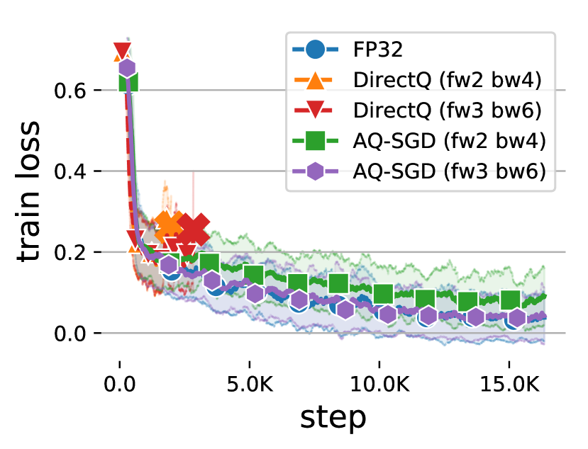
(a) QNLI, DeBERTa-1.5B

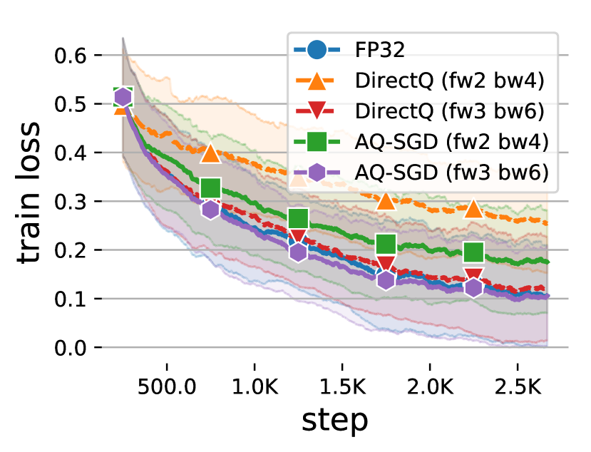
(b) CoLA, DeBERTa-1.5B

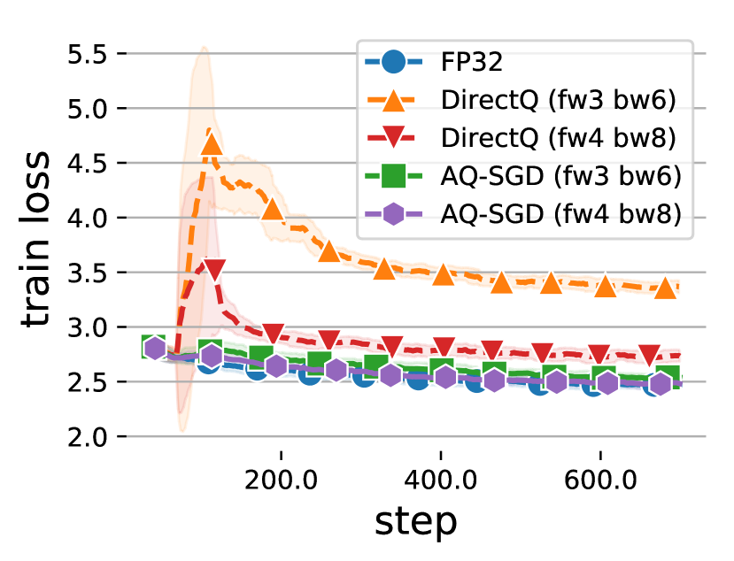
(c) WikiText2, GPT2-1.5B

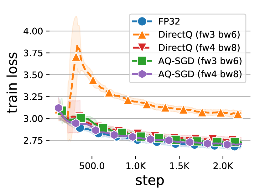
(d) arXiv, GPT2-1.5B

Figure 6: Convergence (loss vs. # stpes) of different approaches. $\boldsymbol{\times}$ represents divergence.

H.2 Throughput under Different Dataset Settings

We show the training throughput under different dataset settings in Figure 5. In general, the observation is similar to that of the main content: our approach maintains similar throughput even when the network is 100$\times$ slower (from 10Gbps to 100Mbps). WikiText2 and arXiv have essentially the same throughput results, since we use the same training settings for them.

Table 5: Training Throughput.

	DeBERTa-1.5B, QNLI			GPT2-1.5B, WikiText2
Network Bandwidth	FP32	DirectQ fw2 bw4 / fw3 bw6	AQ-SGD fw2 bw4 / fw3 bw6	FP32	DirectQ fw3 bw6 / fw4 bw8	AQ-SGD fw3 bw6 / fw4 bw8
10 Gbps	12.9±0.02	13.6±0.02 / 13.6±0.02	13.6±0.02 / 13.5±0.02	3.8±0.01	4.0±0.01 / 4.1±0.01	4.0±0.01 / 4.0±0.01
1 Gbps	9.6±0.02	13.3±0.02 / 13.1±0.02	13.3±0.02 / 13.0±0.02	3.2±0.01	4.0±0.01 / 4.0±0.01	4.0±0.01 / 3.9±0.01
500 Mbps	6.2±0.03	13.0±0.03 / 12.6±0.03	12.9±0.03 / 12.5±0.03	2.7±0.02	3.9±0.01 / 3.9±0.01	3.9±0.01 / 3.9±0.01
300 Mbps	4.4±0.04	12.5±0.02 / 11.9±0.03	12.4±0.03 / 11.8±0.03	1.8±0.02	3.9±0.01 / 3.8±0.01	3.8±0.01 / 3.8±0.01
100 Mbps	1.6±0.04	10.7±0.03 /   9.4±0.03	10.6±0.03 /   9.1±0.03	0.5±0.02	3.5±0.02 / 3.0±0.02	3.4±0.01 / 3.0±0.02

	DeBERTa-1.5B, CoLA			GPT2-1.5B, arXiv
Network Bandwidth	FP32	DirectQ fw2 bw4 / fw3 bw6	AQ-SGD fw2 bw4 / fw3 bw6	FP32	DirectQ fw3 bw6 / fw4 bw8	AQ-SGD fw3 bw6 / fw4 bw8
10 Gbps	17.1±0.03	18.0±0.03 / 17.9±0.03	17.9±0.03 / 17.8±0.03	3.8±0.01	4.0±0.01 / 4.1±0.01	4.0±0.01 / 4.0±0.01
1 Gbps	12.2±0.03	17.4±0.02 / 17.1±0.02	17.3±0.02 / 16.9±0.02	3.2±0.01	4.0±0.01 / 4.0±0.01	4.0±0.01 / 3.9±0.01
500 Mbps	8.9±0.03	16.7±0.03 / 16.2±0.03	16.7±0.03 / 16.1±0.03	2.7±0.02	3.9±0.01 / 3.9±0.01	3.9±0.01 / 3.9±0.01
300 Mbps	6.0±0.04	16.1±0.03 / 15.2±0.03	16.0±0.03 / 15.1±0.03	1.8±0.02	3.9±0.01 / 3.8±0.01	3.8±0.01 / 3.8±0.01
100 Mbps	2.2±0.04	13.1±0.03 / 11.5±0.03	13.1±0.03 / 11.3±0.03	0.5±0.03	3.5±0.01 / 3.0±0.02	3.4±0.01 / 3.0±0.01

H.3 Results of Training from Scratch

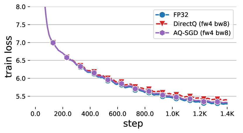
(a) Wiki from scratch

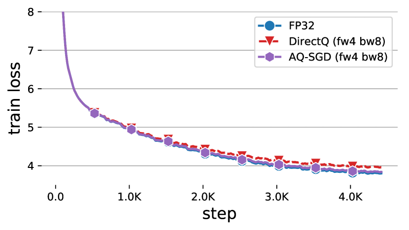
(b) arXiv from scratch

Figure 7: Convergence results of training from scratch.

We investigate the numerical stability of AQ-SGD by showing the convergence result of training from scratch, where the model parameters are randomly initialized. We train WikiText and arXiv datasets for 20 epochs and use the first 10% of steps as warm-up, respectively. As shown in Figure H.3, we can see that AQ-SGD converges almost as fast as FP32 when training from scratch, which indicates our approach is robust enough even when the model is far from the converged state. In contrast, the curve of DirectQ becomes flatter in the late training stage, showing a clear gap with FP32.

H.4 Results of Training under FP16

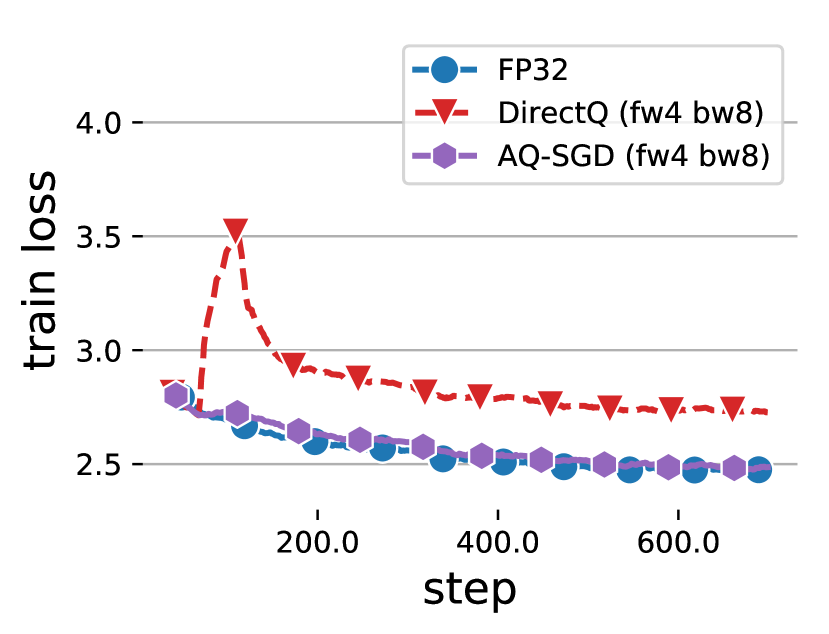
(a) Wiki, FP32

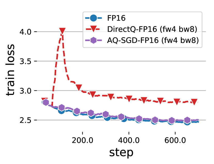
(b) Wiki, FP16

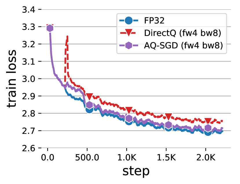
(c) arXiv, FP32

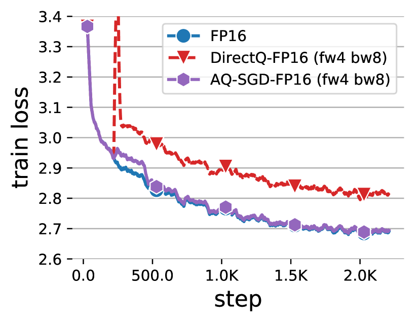
(d) arXiv, FP16

Figure 8: Comparison of fine-tuning under FP32 and FP16.

To investigate the convergence performance of AQ-SGD under low-precision training, we here show the results of FP16 training, and compare it with FP32 training. Figure 8 compares the results under FP32 and FP16. In general, the convergence curves are consistent with the FP32 case. This confirms the effectiveness of AQ-SGD when the activation is already in low precision.

H.5 Hyper-parameter Sensitivity

Here we demonstrate the robustness of our method in various settings. For fast validation, we focus on evaluating DeBERTa-v3-base on QNIL and CoLA datasets. We by default use $K=4$ devices for pipeline parallel training, 2 bits for forward activation, and 4 bits for backward gradients (fw2 bw4).

Number of Pipeline Stages. We first investigate the influence of the number of pipeline stages on convergence performance. Intuitively, partitioning into more pipeline stages leads to more rounds of data compression and communication,resulting in a larger accumulated compression error. The results of Figures 9(a) and 9(b) confirm this intuition. Specifically, the direct quantization method works not bad when $K=2$, but its performance becomes unsatisfied when we further enlarge $K$. In comparison, our approach can maintain similar convergence performance to FP32.

Number of Bits in Communication. Figures 9(c) and 9(d) compare different methods with different numbers of bits in communication. We observe that using more bits can improve the convergence performance but lead to higher communication overheads. In general, our approach achieves better accuracy-efficiency trade-offs.

Number of Bits for Previous Messages. We may find that storing all previous messages is space-intensive. To reduce such requirements, we show that previous messages $m$ can be preserved with low precision. We here perform quantization on $m$, where m$z$ means that we use $z$ bits for previous messages. Figures 9(e) and 9(f) show the results with different number of bits of the previous messages. When only $2$ bits are used for the previous messages, despite the fact that it is slightly worse than our default setting, our approach is still significantly better than DirectQ. And there is no significant performance drop when $8$ bits are used for the previous messages.

Pre-trained Model Sizes. Figures 9(g) and 9(h) show the results of the base and large version of DeBERTa. Surprisingly, larger models seem to be more tolerant of errors from activation compression than smaller models. One possible reason is that larger models usually use much smaller learning rates. So the error of each iteration can be restricted to a smaller range. Here, we use 2.0e-5 for the base model and 7e-6 for the large model, as suggested in the official repository of DeBERTa.

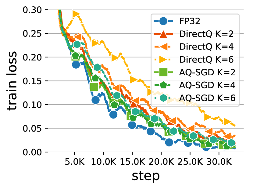
(a) QNLI, $K$ stages

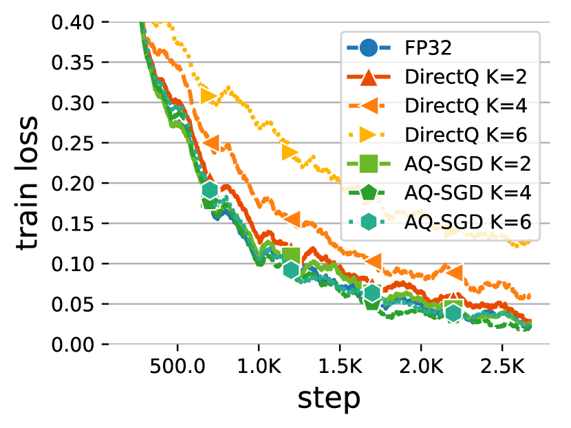
(b) CoLA, $K$ stages

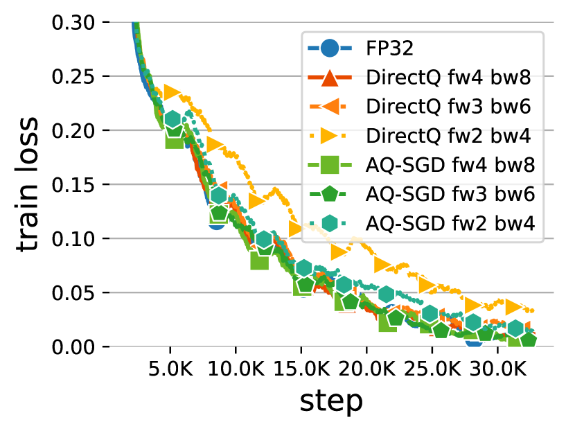
(c) QNLI, $n$ bits

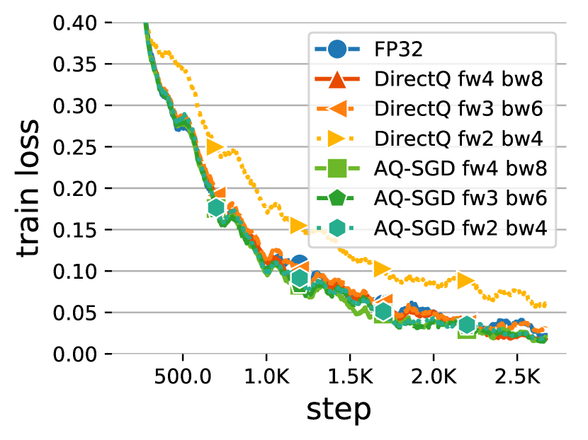
(d) CoLA, $n$ bits

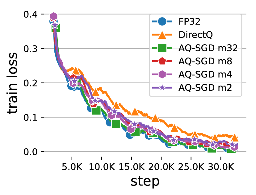
(e) QNLI, low-bit $m$

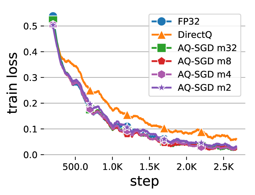
(f) CoLA, low-bit $m$

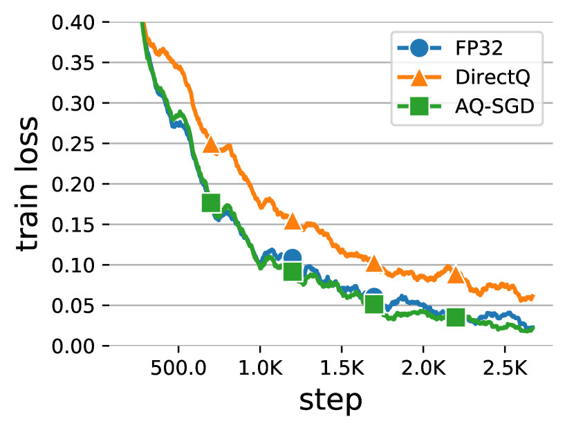
(g) CoLA, DeBERTa-base

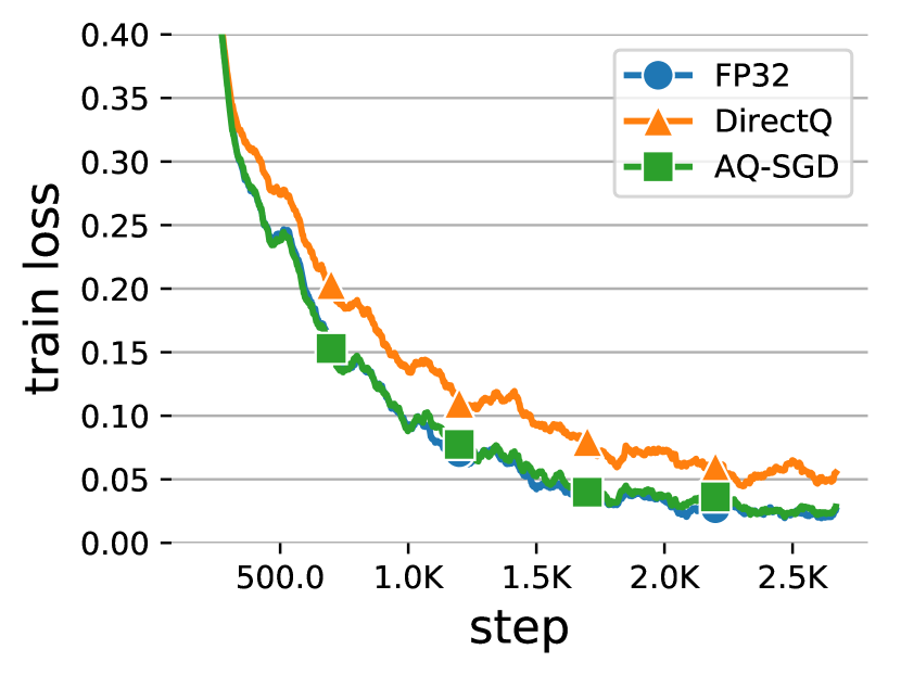
(h) CoLA, DeBERTa-large

Figure 9: Convergence curves under different configurations.

H.6 Split Learning

Split learning is a scenario of federated learning, where the client trains a shallow part of deep network (known as the cut layer) that accesses the training data, while the rest of the model is trained in a data center. Clients and server need to exchange the activation and its gradients in the cut, where AQ-SGD can be adopted. We evaluated AQ-SGD on a split learning scenario where neither the input data nor its labels are shared with the server—the model is cut twice, one after the first resnet block and one before the last block to generate the prediction. We evaluate AQ-SGD for split learning over Cifar10 and Cifar100 with the ResNet34 model. We set 16 clients and use a Dirichlet distribution with concentration parameter 0.5 to synthesize non-identical datasets. Following the previously established work of split learning, in each communication round, we conduct local training for each client sequentially. and each client will train 3 epochs with its local data. We utilize SGD optimizer with momentum of 0.9, a batch size of 64, and a learning rate of 0.01. We decay the learning rate to its 10% for every 20 communication rounds.

The datasets are augmented with random cropping and flipping. To adapt to random cropping, we do the same cropping operation on the retrieved previous message, and only update its non-cropped part. To adapt to random flipping, we maintain another previous message copy for flipped images, and retrieve and update only the corresponding copy during training.

Figure 10 presents the results of split learning, where fw2 bw8[0.2] means that, for forward pass, we perform 2-bit quantization, and for backward pass, we keep only the top 20% gradients and then perform 8-bit quantization. We can see that AQ-SGD transfers the activations in 2 bits while maintaining a performance similar to FP32, which indicates the effectiveness of AQ-SGD in improving the communication efficiency in the split learning scenario. Furthermore, compared to DirectQ, AQ-SGD shows advantages in terms of both the convergence and generalization of the trained model.

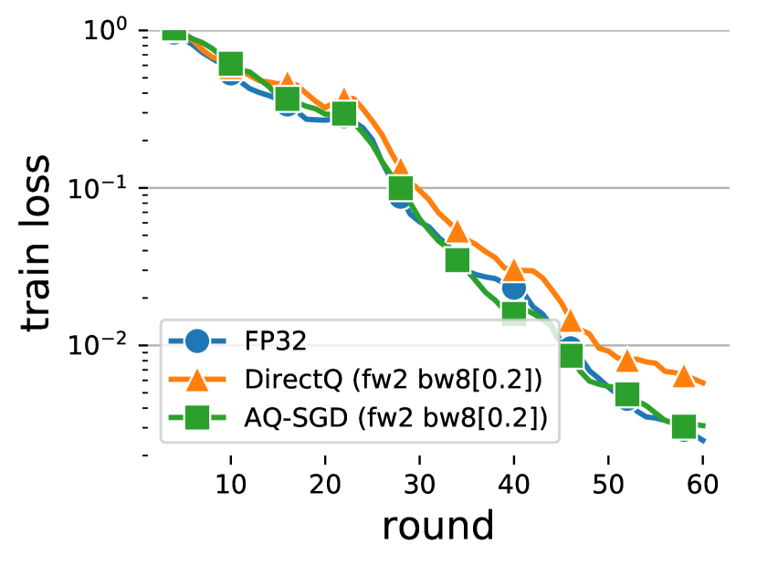
(a) Cifar10, Train Loss

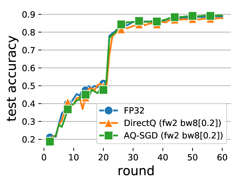
(b) Cifar10, Test ACC

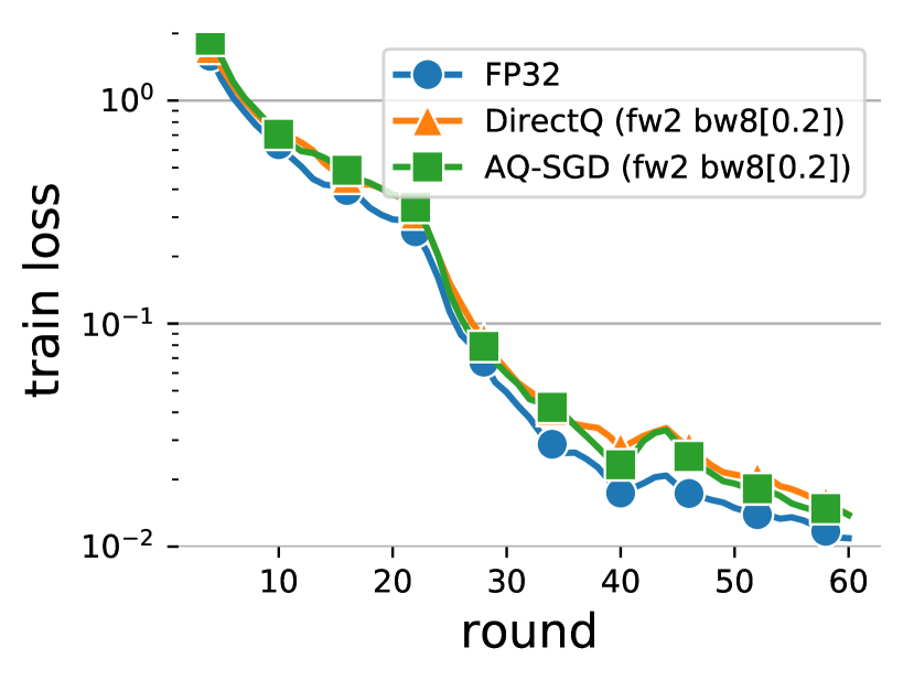
(c) Cifar100, Train Loss

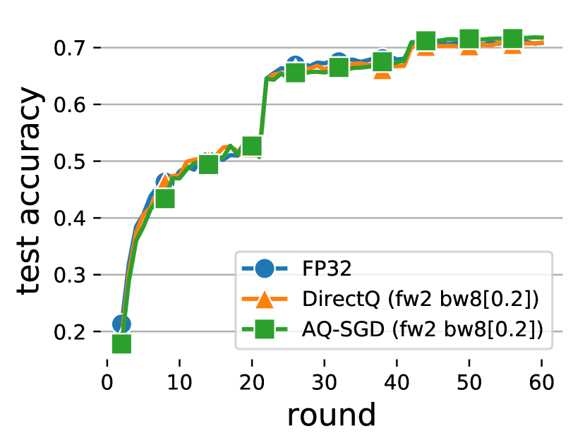
(d) Cifar100, Test ACC

Figure 10: Results of split learning with ResNet34.

Appendix I Case Study of Generation Results

We here conduct case study to better understand the generation quality across different methods. All methods are fine-tuned on WikiText with the same seed. We use greedy decoding to generate texts. For DirectQ and AQ-SGD, we use 4-bit in forward pass and 8-bit in backward pass.

We randomly pick documents from the test set of WikiText to construct the prompts and let the model complete the rest. The generation results after fine-tuning are presented in Tables 6 and 7. For instance, in Cases 1 and 2, AQ-SGD produces the same results as FP32; in Case 3, although AQ-SGD does not generate the exact same output as FP32, it still expresses a similar meaning. This indicates our proposed compression scheme has relatively little impact on the learning process. In contrast, DirectQ may generate text that is not relevant to the context. For example, in Case 1, we know that “Matsuo Bashō was strongly influenced by Du Fu”, so we should expect the text below to show the fact how he was influenced, just like FP32 and AQ-SGD did. But DirectQ fails to generate reasonable text based on the context. Other inference results presented in Tables 6 and 7 lead to the same observation.

Table 6: Case study of generation results.

Case 1
Prompt:	… Matsuo Bashō, the greatest haiku poet, was also strongly influenced by Du Fu; in Oku no Hosomichi, his masterpiece, he cites the first two lines of A Spring View before a haiku as its introduction and also many of his other haiku have similar wording and themes. It is said that when he died
Gold:	in Osaka during a long travel, a copy of Du Fu’s poetry was found with him as one of a few precious items which he was able to carry around.
FP32:	, his body was placed in a coffin with a Du Fu-like inscription.
AQ-SGD:	, his body was placed in a coffin with a Du Fu-like inscription.
DirectQ:	, his body was covered with a red cloth and his head was shaved.
Case 2
Prompt:	… Peppiatt notes that the exhibition showed Bacon no longer needed sensationalist material to make an impact, and was now
Gold:	capable of creating an intense emotional response through more subtle means …
FP32:	able to "make a serious contribution to the art of painting"
AQ-SGD:	able to "make a serious contribution to the art of painting"
DirectQ:	able to "make a serious statement about the state of the art"
Case 3
Prompt:	… At this point, Dokhturov’s column appeared behind the French line and joined the battle. The French were outnumbered more than three to
Gold:	one, assaulted in the front by Miloradovich’s column, in the middle by Strik’s and in the rear by Dokhturov.
FP32:	one, but they held their ground and forced the Russians to retreat.
AQ-SGD:	one, but they were able to hold their ground.
DirectQ:	one, and the Russians were able to hold their ground.
Case 4
Prompt:	… Between Jupiter and Fort Pierce, the storm knocked down power and telegraph lines. In the latter city, high waves washed out a portion of the causeway. In the 1980s, an elderly resident recalled that the storm was the
Gold:	most severe on record in Fort Pierce.
FP32:	worst storm he had ever seen.
AQ-SGD:	worst storm he had ever seen.
DirectQ:	worst he had ever experienced.
Case 5
Prompt:	… Lesnar was born in Webster, South Dakota, on July 12, 1977. He was raised on a Webster dairy farm owned by his parents, Stephanie and Richard Lesnar. He is of German descent. He has two older brothers named Troy and Chad, and a younger sister named Brandi. At age 17, he joined the National Guard, where he
Gold:	was assigned to an office job after his red-green colorblindness was deemed hazardous to his desire to work with explosives.
FP32:	served in the South Dakota National Guard. He was a member of the South Dakota National Guard for two years.
AQ-SGD:	served in the South Dakota National Guard. He was a member of the South Dakota National Guard for two years.
DirectQ:	served in the South Dakota National Guard for two years. He was discharged in May 1991.

Table 7: Case study of generation results (more).

Case 6
Prompt:	… Mega placed the game at # 7 in their "Top Mega Drive Games of All Time" list. MegaTech magazine praised the game’s graphics, but criticized the game’s easy difficulty level,
Gold:	explaining simply that "the graphics are excellent, but the game is easy to complete."
FP32:	stating that "the game is too easy to be enjoyable".
AQ-SGD:	stating that it was "too easy".
DirectQ:	which was criticized for being too easy.
Case 7
Prompt:	… "Obviously, he has great rapport and communication ability with his team." Yahoo! Sports compared Stevens to legendary coach John Wooden writing "
Gold:	Brad Stevens is winning at Butler the Wooden way – calm and composed on the sideline."
FP32:	He’s a coach who has been around the block, and he’s not afraid to tell you what he thinks."
AQ-SGD:	Stevens is a coach who has been around the game for a long time, and he has a knack for getting the most out of his players."
DirectQ:	Stevens is a coach who has been able to mold a team into a championship contender. He has a knack for getting the most out of his players, and he has a knack for getting the most out of his players’ personalities."
Case 8
Prompt:	… The Gore’s social circle in England revolved around his good friend Rufus King, who
Gold:	was appointed Ambassador to Great Britain in 1796, along with other Massachusetts expatriates.
FP32:	was a member of the Royal Society.
AQ-SGD:	was a member of the Royal Society.
DirectQ:	was a member of the Royal Society.
Case 9
Prompt:	… The city has 896 barangays that are known by sequential numbers instead of names. These barangays are further group into
Gold:	100 zones for administrative and municipal purposes.
FP32:	districts, which are further subdivided into wards.
AQ-SGD:	districts, which are further subdivided into wards.
DirectQ:	districts, which are numbered according to the number of barangays in the district.
Case 10
Prompt:	… The National Spiritual Assembly of the Bahá ’ís of the Philippines, the governing body of the Filipino Bahá’í community, is
Gold:	headquartered near Manila’s eastern border with Makati.
FP32:	headquartered in the city.
AQ-SGD:	headquartered in the city.
DirectQ:	headquartered in the city.

References

- Ryabinin and Gusev [2020] Max Ryabinin and Anton Gusev. Towards crowdsourced training of large neural networks using decentralized mixture-of-experts. Advances in Neural Information Processing Systems, 33:3659–3672, 2020.
- Diskin et al. [2021] Michael Diskin, Alexey Bukhtiyarov, Max Ryabinin, Lucile Saulnier, Anton Sinitsin, Dmitry Popov, Dmitry V Pyrkin, Maxim Kashirin, Alexander Borzunov, Albert Villanova del Moral, et al. Distributed deep learning in open collaborations. Advances in Neural Information Processing Systems, 34:7879–7897, 2021.
- Borzunov et al. [2022] Alexander Borzunov, Max Ryabinin, Tim Dettmers, Quentin Lhoest, Lucile Saulnier, Michael Diskin, and Yacine Jernite. Training transformers together. In NeurIPS 2021 Competitions and Demonstrations Track, pages 335–342. PMLR, 2022.
- Ryabinin et al. [2023] Max Ryabinin, Tim Dettmers, Michael Diskin, and Alexander Borzunov. Swarm parallelism: Training large models can be surprisingly communication-efficient. 2023.
- Alistarh et al. [2016] Dan Alistarh, Demjan Grubic, Jerry Li, Ryota Tomioka, and Milan Vojnovic. Qsgd: Communication-efficient sgd via gradient quantization and encoding. arXiv preprint arXiv:1610.02132, 2016.
- Zhang et al. [2017] Hantian Zhang, Jerry Li, Kaan Kara, Dan Alistarh, Ji Liu, and Ce Zhang. Zipml: Training linear models with end-to-end low precision, and a little bit of deep learning. In International Conference on Machine Learning, pages 4035–4043. PMLR, 2017.
- Bernstein et al. [2018] Jeremy Bernstein, Yu-Xiang Wang, Kamyar Azizzadenesheli, and Animashree Anandkumar. signsgd: Compressed optimisation for non-convex problems. In International Conference on Machine Learning, pages 560–569. PMLR, 2018.
- Wen et al. [2017] Wei Wen, Cong Xu, Feng Yan, Chunpeng Wu, Yandan Wang, Yiran Chen, and Hai Li. Terngrad: ternary gradients to reduce communication in distributed deep learning. In Proceedings of the 31st International Conference on Neural Information Processing Systems, pages 1508–1518, 2017.
- Koloskova et al. [2019] Anastasia Koloskova, Sebastian Stich, and Martin Jaggi. Decentralized stochastic optimization and gossip algorithms with compressed communication. In International Conference on Machine Learning, pages 3478–3487. PMLR, 2019.
- Li et al. [2018] Youjie Li, Mingchao Yu, Songze Li, Salman Avestimehr, Nam Sung Kim, and Alexander Schwing. Pipe-sgd: a decentralized pipelined sgd framework for distributed deep net training. In Proceedings of the 32nd International Conference on Neural Information Processing Systems, pages 8056–8067, 2018.
- Lian et al. [2017] Xiangru Lian, Ce Zhang, Huan Zhang, Cho-Jui Hsieh, Wei Zhang, and Ji Liu. Can decentralized algorithms outperform centralized algorithms? a case study for decentralized parallel stochastic gradient descent. In Proceedings of the 31st International Conference on Neural Information Processing Systems, pages 5336–5346, 2017.
- Lian et al. [2018] Xiangru Lian, Wei Zhang, Ce Zhang, and Ji Liu. Asynchronous decentralized parallel stochastic gradient descent. In International Conference on Machine Learning, pages 3043–3052. PMLR, 2018.
- Tang et al. [2018a] Hanlin Tang, Shaoduo Gan, Ce Zhang, Tong Zhang, and Ji Liu. Communication compression for decentralized training. In Proceedings of the 32nd International Conference on Neural Information Processing Systems, pages 7663–7673, 2018a.
- Tang et al. [2018b] Hanlin Tang, Xiangru Lian, Ming Yan, Ce Zhang, and Ji Liu. D2: Decentralized training over decentralized data. In International Conference on Machine Learning, pages 4848–4856. PMLR, 2018b.
- [15] Shen Li, Yanli Zhao, Rohan Varma, Omkar Salpekar, Pieter Noordhuis, Teng Li, Adam Paszke, Jeff Smith, Brian Vaughan, Pritam Damania, et al. Pytorch distributed: Experiences on accelerating data parallel training. Proceedings of the VLDB Endowment, 13(12).
- [16] Pytorch-lightning. https://www.pytorchlightning.ai/.
- Sergeev and Del Balso [2018] Alexander Sergeev and Mike Del Balso. Horovod: fast and easy distributed deep learning in tensorflow. arXiv preprint arXiv:1802.05799, 2018.
- Gan, Shaoduo and Lian, Xiangru and Wang, Rui and Chang, Jianbin and Liu, Chengjun and Shi, Hongmei and Zhang, Shengzhuo and Li, Xianghong and Sun, Tengxu and Jiang, Jiawei and others [2021] Gan, Shaoduo and Lian, Xiangru and Wang, Rui and Chang, Jianbin and Liu, Chengjun and Shi, Hongmei and Zhang, Shengzhuo and Li, Xianghong and Sun, Tengxu and Jiang, Jiawei and others. BAGUA: scaling up distributed learning with system relaxations. Proceedings of the VLDB Endowment, 15(4):804–813, 2021.
- Jiang et al. [2020] Yimin Jiang, Yibo Zhu, Chang Lan, Bairen Yi, Yong Cui, and Chuanxiong Guo. A unified architecture for accelerating distributed DNN training in heterogeneous gpu/cpu clusters. In 14th USENIX Symposium on Operating Systems Design and Implementation (OSDI 20), pages 463–479, 2020.
- Bommasani et al. [2021] Rishi Bommasani, Drew A. Hudson, Ehsan Adeli, Russ Altman, Simran Arora, Sydney von Arx, Michael S. Bernstein, Jeannette Bohg, Antoine Bosselut, Emma Brunskill, Erik Brynjolfsson, Shyamal Buch, Dallas Card, Rodrigo Castellon, Niladri S. Chatterji, Annie S. Chen, Kathleen Creel, Jared Quincy Davis, Dorottya Demszky, Chris Donahue, Moussa Doumbouya, Esin Durmus, Stefano Ermon, John Etchemendy, Kawin Ethayarajh, Li Fei-Fei, Chelsea Finn, Trevor Gale, Lauren Gillespie, Karan Goel, Noah D. Goodman, Shelby Grossman, Neel Guha, Tatsunori Hashimoto, Peter Henderson, John Hewitt, Daniel E. Ho, Jenny Hong, Kyle Hsu, Jing Huang, Thomas Icard, Saahil Jain, Dan Jurafsky, Pratyusha Kalluri, Siddharth Karamcheti, Geoff Keeling, Fereshte Khani, Omar Khattab, Pang Wei Koh, Mark S. Krass, Ranjay Krishna, Rohith Kuditipudi, and et al. On the opportunities and risks of foundation models. CoRR, abs/2108.07258, 2021. URL https://arxiv.org/abs/2108.07258.
- Devlin et al. [2018] Jacob Devlin, Ming-Wei Chang, Kenton Lee, and Kristina Toutanova. Bert: Pre-training of deep bidirectional transformers for language understanding. arXiv preprint arXiv:1810.04805, 2018.
- Brown et al. [2020] Tom Brown, Benjamin Mann, Nick Ryder, Melanie Subbiah, Jared D Kaplan, Prafulla Dhariwal, Arvind Neelakantan, Pranav Shyam, Girish Sastry, Amanda Askell, et al. Language models are few-shot learners. Advances in neural information processing systems, 33:1877–1901, 2020.
- Radford et al. [2021] Alec Radford, Jong Wook Kim, Chris Hallacy, Aditya Ramesh, Gabriel Goh, Sandhini Agarwal, Girish Sastry, Amanda Askell, Pamela Mishkin, Jack Clark, et al. Learning transferable visual models from natural language supervision. In International Conference on Machine Learning, pages 8748–8763. PMLR, 2021.
- Shoeybi et al. [2019] Mohammad Shoeybi, Mostofa Patwary, Raul Puri, Patrick LeGresley, Jared Casper, and Bryan Catanzaro. Megatron-lm: Training multi-billion parameter language models using model parallelism. arXiv preprint arXiv:1909.08053, 2019.
- Rasley et al. [2020] Jeff Rasley, Samyam Rajbhandari, Olatunji Ruwase, and Yuxiong He. Deepspeed: System optimizations enable training deep learning models with over 100 billion parameters. In Proceedings of the 26th ACM SIGKDD International Conference on Knowledge Discovery & Data Mining, pages 3505–3506, 2020.
- Baines et al. [2021] Mandeep Baines, Shruti Bhosale, Vittorio Caggiano, Naman Goyal, Siddharth Goyal, Myle Ott, Benjamin Lefaudeux, Vitaliy Liptchinsky, Mike Rabbat, Sam Sheiffer, et al. Fairscale: A general purpose modular pytorch library for high performance and large scale training, 2021.
- Tang et al. [2019a] Hanlin Tang, Chen Yu, Xiangru Lian, Tong Zhang, and Ji Liu. Doublesqueeze: Parallel stochastic gradient descent with double-pass error-compensated compression. In International Conference on Machine Learning, pages 6155–6165. PMLR, 2019a.
- Tang et al. [2019b] Hanlin Tang, Xiangru Lian, Shuang Qiu, Lei Yuan, Ce Zhang, Tong Zhang, and Ji Liu. Deepsqueeze: Parallel stochastic gradient descent with double-pass error-compensated compression. arXiv preprint arXiv:1907.07346, 2019b.
- Evans and Aamodt [2021] R David Evans and Tor Aamodt. Ac-gc: Lossy activation compression with guaranteed convergence. Advances in Neural Information Processing Systems, 34, 2021.
- Fu et al. [2020] Fangcheng Fu, Yuzheng Hu, Yihan He, Jiawei Jiang, Yingxia Shao, Ce Zhang, and Bin Cui. Don’t waste your bits! squeeze activations and gradients for deep neural networks via tinyscript. In International Conference on Machine Learning, pages 3304–3314. PMLR, 2020.
- Bottou et al. [2018] Léon Bottou, Frank E Curtis, and Jorge Nocedal. Optimization methods for large-scale machine learning. Siam Review, 60(2):223–311, 2018.
- Han et al. [2016] Song Han, Huizi Mao, and William J Dally. Deep compression: Compressing deep neural networks with pruning, trained quantization and huffman coding. 2016.
- Hubara et al. [2017] Itay Hubara, Matthieu Courbariaux, Daniel Soudry, Ran El-Yaniv, and Yoshua Bengio. Quantized neural networks: Training neural networks with low precision weights and activations. The Journal of Machine Learning Research, 18(1):6869–6898, 2017.
- Jain et al. [2018] Animesh Jain, Amar Phanishayee, Jason Mars, Lingjia Tang, and Gennady Pekhimenko. Gist: Efficient data encoding for deep neural network training. In 2018 ACM/IEEE 45th Annual International Symposium on Computer Architecture (ISCA), pages 776–789. IEEE, 2018.
- Chakrabarti and Moseley [2019] Ayan Chakrabarti and Benjamin Moseley. Backprop with approximate activations for memory-efficient network training. Advances in Neural Information Processing Systems, 32, 2019.
- Chen et al. [2021a] Jianfei Chen, Lianmin Zheng, Zhewei Yao, Dequan Wang, Ion Stoica, Michael Mahoney, and Joseph Gonzalez. Actnn: Reducing training memory footprint via 2-bit activation compressed training. In International Conference on Machine Learning, pages 1803–1813. PMLR, 2021a.
- Liu and Zhang [2021] Ji Liu and Ce Zhang. Distributed learning systems with first-order methods. arXiv preprint arXiv:2104.05245, 2021.
- Ajalloeian and Stich [2020] Ahmad Ajalloeian and Sebastian U. Stich. On the convergence of sgd with biased gradients, 2020. URL https://arxiv.org/abs/2008.00051.
- Kingma and Ba [2015] Diederik P. Kingma and Jimmy Ba. Adam: A method for stochastic optimization. In Yoshua Bengio and Yann LeCun, editors, 3rd International Conference on Learning Representations, ICLR 2015, San Diego, CA, USA, May 7-9, 2015, Conference Track Proceedings, 2015. URL http://arxiv.org/abs/1412.6980.
- Tang et al. [2021] Hanlin Tang, Shaoduo Gan, Ammar Ahmad Awan, Samyam Rajbhandari, Conglong Li, Xiangru Lian, Ji Liu, Ce Zhang, and Yuxiong He. 1-bit adam: Communication efficient large-scale training with adam’s convergence speed. In International Conference on Machine Learning, pages 10118–10129. PMLR, 2021.
- Huang et al. [2019] Yanping Huang, Youlong Cheng, Ankur Bapna, Orhan Firat, Dehao Chen, Mia Chen, HyoukJoong Lee, Jiquan Ngiam, Quoc V Le, Yonghui Wu, et al. Gpipe: Efficient training of giant neural networks using pipeline parallelism. Advances in neural information processing systems, 32, 2019.
- Yang et al. [2021] Bowen Yang, Jian Zhang, Jonathan Li, Christopher Ré, Christopher Aberger, and Christopher De Sa. Pipemare: Asynchronous pipeline parallel dnn training. Proceedings of Machine Learning and Systems, 3:269–296, 2021.
- Narayanan et al. [2019] Deepak Narayanan, Aaron Harlap, Amar Phanishayee, Vivek Seshadri, Nikhil R Devanur, Gregory R Ganger, Phillip B Gibbons, and Matei Zaharia. Pipedream: generalized pipeline parallelism for dnn training. In Proceedings of the 27th ACM Symposium on Operating Systems Principles, pages 1–15, 2019.
- Narayanan et al. [2021] Deepak Narayanan, Amar Phanishayee, Kaiyu Shi, Xie Chen, and Matei Zaharia. Memory-efficient pipeline-parallel dnn training. In International Conference on Machine Learning, pages 7937–7947. PMLR, 2021.
- Chen et al. [2020] Chia-Yu Chen, Jiamin Ni, Songtao Lu, Xiaodong Cui, Pin-Yu Chen, Xiao Sun, Naigang Wang, Swagath Venkataramani, Vijayalakshmi Viji Srinivasan, Wei Zhang, et al. Scalecom: Scalable sparsified gradient compression for communication-efficient distributed training. Advances in Neural Information Processing Systems, 33:13551–13563, 2020.
- Xie et al. [2020] Cong Xie, Shuai Zheng, Sanmi Koyejo, Indranil Gupta, Mu Li, and Haibin Lin. Cser: Communication-efficient sgd with error reset. Advances in Neural Information Processing Systems, 33:12593–12603, 2020.
- Faghri et al. [2020] Fartash Faghri, Iman Tabrizian, Ilia Markov, Dan Alistarh, Daniel M Roy, and Ali Ramezani-Kebrya. Adaptive gradient quantization for data-parallel sgd. Advances in neural information processing systems, 33:3174–3185, 2020.
- Li et al. [2020] Zhize Li, Dmitry Kovalev, Xun Qian, and Peter Richtarik. Acceleration for compressed gradient descent in distributed and federated optimization. In International Conference on Machine Learning, pages 5895–5904. PMLR, 2020.
- Rothchild et al. [2020] Daniel Rothchild, Ashwinee Panda, Enayat Ullah, Nikita Ivkin, Ion Stoica, Vladimir Braverman, Joseph Gonzalez, and Raman Arora. Fetchsgd: Communication-efficient federated learning with sketching. In International Conference on Machine Learning, pages 8253–8265. PMLR, 2020.
- Safaryan and Richtárik [2021] Mher Safaryan and Peter Richtárik. Stochastic sign descent methods: New algorithms and better theory. In International Conference on Machine Learning, pages 9224–9234. PMLR, 2021.
- Gorbunov et al. [2021] Eduard Gorbunov, Konstantin P Burlachenko, Zhize Li, and Peter Richtárik. Marina: Faster non-convex distributed learning with compression. In International Conference on Machine Learning, pages 3788–3798. PMLR, 2021.
- Safaryan et al. [2021] Mher Safaryan, Filip Hanzely, and Peter Richtárik. Smoothness matrices beat smoothness constants: better communication compression techniques for distributed optimization. Advances in Neural Information Processing Systems, 34, 2021.
- Qian et al. [2021] Xun Qian, Peter Richtárik, and Tong Zhang. Error compensated distributed sgd can be accelerated. Advances in Neural Information Processing Systems, 34, 2021.
- M Abdelmoniem et al. [2021] Ahmed M Abdelmoniem, Ahmed Elzanaty, Mohamed-Slim Alouini, and Marco Canini. An efficient statistical-based gradient compression technique for distributed training systems. Proceedings of Machine Learning and Systems, 3:297–322, 2021.
- Wang et al. [2021] Hongyi Wang, Saurabh Agarwal, and Dimitris Papailiopoulos. Pufferfish: Communication-efficient models at no extra cost. Proceedings of Machine Learning and Systems, 3:365–386, 2021.
- Wangni et al. [2018] J Wangni, J Liu, J Wang, and T Zhang. Gradient sparsification for communication-efficient distributed optimization. Advances in Neural Information Processing Systems, 31:1299, 2018.
- Alistarh et al. [2018] Dan Alistarh, Torsten Hoefler, Mikael Johansson, Sarit Khirirat, Nikola Konstantinov, and Cédric Renggli. The convergence of sparsified gradient methods. In Proceedings of the 32nd International Conference on Neural Information Processing Systems, pages 5977–5987, 2018.
- Wang et al. [2018] Hongyi Wang, Scott Sievert, Zachary Charles, Shengchao Liu, Stephen Wright, and Dimitris Papailiopoulos. Atomo: communication-efficient learning via atomic sparsification. In Proceedings of the 32nd International Conference on Neural Information Processing Systems, pages 9872–9883, 2018.
- Wang et al. [2017] Jialei Wang, Mladen Kolar, Nathan Srebro, and Tong Zhang. Efficient distributed learning with sparsity. In International Conference on Machine Learning, pages 3636–3645. PMLR, 2017.
- Jiang et al. [2018] Jiawei Jiang, Fangcheng Fu, Tong Yang, and Bin Cui. Sketchml: Accelerating distributed machine learning with data sketches. In Proceedings of the 2018 ACM SIGMOD International Conference on Management of Data, pages 1269–1284, 2018.
- Ivkin et al. [2019] Nikita Ivkin, Daniel Rothchild, Enayat Ullah, Ion Stoica, Raman Arora, et al. Communication-efficient distributed sgd with sketching. In Advances in Neural Information Processing Systems, pages 13144–13154, 2019.
- Mocanu et al. [2018] Decebal Constantin Mocanu, Elena Mocanu, Peter Stone, Phuong H Nguyen, Madeleine Gibescu, and Antonio Liotta. Scalable training of artificial neural networks with adaptive sparse connectivity inspired by network science. Nature communications, 9(1):1–12, 2018.
- Raihan and Aamodt [2020] Md Aamir Raihan and Tor Aamodt. Sparse weight activation training. Advances in Neural Information Processing Systems, 33:15625–15638, 2020.
- Chen et al. [2021b] Beidi Chen, Tri Dao, Kaizhao Liang, Jiaming Yang, Zhao Song, Atri Rudra, and Christopher Re. Pixelated butterfly: Simple and efficient sparse training for neural network models. arXiv preprint arXiv:2112.00029, 2021b.
- Dettmers and Zettlemoyer [2019] Tim Dettmers and Luke Zettlemoyer. Sparse networks from scratch: Faster training without losing performance. arXiv preprint arXiv:1907.04840, 2019.
- Mostafa and Wang [2019] Hesham Mostafa and Xin Wang. Parameter efficient training of deep convolutional neural networks by dynamic sparse reparameterization. In International Conference on Machine Learning, pages 4646–4655. PMLR, 2019.
- Junjie et al. [2019] LIU Junjie, XU Zhe, SHI Runbin, Ray CC Cheung, and Hayden KH So. Dynamic sparse training: Find efficient sparse network from scratch with trainable masked layers. In International Conference on Learning Representations, 2019.
- Hoefler et al. [2021] Torsten Hoefler, Dan Alistarh, Tal Ben-Nun, Nikoli Dryden, and Alexandra Peste. Sparsity in deep learning: Pruning and growth for efficient inference and training in neural networks. Journal of Machine Learning Research, 22(241):1–124, 2021.
- Liu et al. [2021a] Shiwei Liu, Tianlong Chen, Xiaohan Chen, Zahra Atashgahi, Lu Yin, Huanyu Kou, Li Shen, Mykola Pechenizkiy, Zhangyang Wang, and Decebal Constantin Mocanu. Sparse training via boosting pruning plasticity with neuroregeneration. Advances in Neural Information Processing Systems, 34, 2021a.
- Choukse et al. [2020] Esha Choukse, Michael B Sullivan, Mike O’Connor, Mattan Erez, Jeff Pool, David Nellans, and Stephen W Keckler. Buddy compression: Enabling larger memory for deep learning and hpc workloads on gpus. In 2020 ACM/IEEE 47th Annual International Symposium on Computer Architecture (ISCA), pages 926–939. IEEE, 2020.
- Rhu et al. [2018] Minsoo Rhu, Mike O’Connor, Niladrish Chatterjee, Jeff Pool, Youngeun Kwon, and Stephen W Keckler. Compressing dma engine: Leveraging activation sparsity for training deep neural networks. In 2018 IEEE International Symposium on High Performance Computer Architecture (HPCA), pages 78–91. IEEE, 2018.
- Lascorz et al. [2019] Alberto Delmás Lascorz, Sayeh Sharify, Isak Edo, Dylan Malone Stuart, Omar Mohamed Awad, Patrick Judd, Mostafa Mahmoud, Milos Nikolic, Kevin Siu, Zissis Poulos, et al. Shapeshifter: Enabling fine-grain data width adaptation in deep learning. In Proceedings of the 52nd Annual IEEE/ACM International Symposium on Microarchitecture, pages 28–41, 2019.
- Jin et al. [2021] Sian Jin, Guanpeng Li, Shuaiwen Leon Song, and Dingwen Tao. A novel memory-efficient deep learning training framework via error-bounded lossy compression. In Proceedings of the 26th ACM SIGPLAN Symposium on Principles and Practice of Parallel Programming, pages 485–487, 2021.
- Evans et al. [2020] R David Evans, Lufei Liu, and Tor M Aamodt. Jpeg-act: accelerating deep learning via transform-based lossy compression. In 2020 ACM/IEEE 47th Annual International Symposium on Computer Architecture (ISCA), pages 860–873. IEEE, 2020.
- Georgiadis [2019] Georgios Georgiadis. Accelerating convolutional neural networks via activation map compression. In Proceedings of the IEEE/CVF Conference on Computer Vision and Pattern Recognition, pages 7085–7095, 2019.
- Gudovskiy et al. [2018] Denis Gudovskiy, Alec Hodgkinson, and Luca Rigazio. Dnn feature map compression using learned representation over gf (2). In Proceedings of the European Conference on Computer Vision (ECCV) Workshops, pages 0–0, 2018.
- Liu et al. [2021b] Zirui Liu, Kaixiong Zhou, Fan Yang, Li Li, Rui Chen, and Xia Hu. Exact: Scalable graph neural networks training via extreme activation compression. In International Conference on Learning Representations, 2021b.
- Pekhimenko et al. [2012] Gennady Pekhimenko, Vivek Seshadri, Onur Mutlu, Michael A Kozuch, Phillip B Gibbons, and Todd C Mowry. Base-delta-immediate compression: Practical data compression for on-chip caches. In 2012 21st international conference on parallel architectures and compilation techniques (PACT), pages 377–388. IEEE, 2012.
- Awad et al. [2021] Omar Mohamed Awad, Mostafa Mahmoud, Isak Edo, Ali Hadi Zadeh, Ciaran Bannon, Anand Jayarajan, Gennady Pekhimenko, and Andreas Moshovos. Fpraker: A processing element for accelerating neural network training. In MICRO-54: 54th Annual IEEE/ACM International Symposium on Microarchitecture, pages 857–869, 2021.
- Bersatti et al. [2020] Andrei Bersatti, Nima Shoghi Ghalehshahi, and Hyesoon Kim. Neural network weight compression with nnw-bdi. In The International Symposium on Memory Systems, pages 335–340, 2020.