A memory-efficient neural ordinary differential equation framework based on high-level adjoint differentiation

Abstract

Neural ordinary differential equations (neural ODEs) have emerged as a novel network architecture that bridges dynamical systems and deep learning. However, the gradient obtained with the continuous adjoint method in the vanilla neural ODE is not reverse-accurate. Other approaches suffer either from an excessive memory requirement due to deep computational graphs or from limited choices for the time integration scheme, hampering their application to large-scale complex dynamical systems. To achieve accurate gradients without compromising memory efficiency and flexibility, we present a new neural ODE framework, PNODE, based on high-level discrete adjoint algorithmic differentiation. By leveraging discrete adjoint time integrators and advanced checkpointing strategies tailored for these integrators, PNODE can provide a balance between memory and computational costs, while computing the gradients consistently and accurately. We provide an open-source implementation based on PyTorch and PETSc, one of the most commonly used portable, scalable scientific computing libraries. We demonstrate the performance through extensive numerical experiments on image classification and continuous normalizing flow problems. We show that PNODE achieves the highest memory efficiency when compared with other reverse-accurate methods. On the image classification problems, PNODE is up to two times faster than the vanilla neural ODE and up to $2.3$ times faster than the best existing reverse-accurate method. We also show that PNODE enables the use of the implicit time integration methods that are needed for stiff dynamical systems.

Keywords Neural ODEs, deep learning, adjoint differentiation, checkpointing, implicit methods

1 Introduction

A residual network can be seen as a forward Euler discretization of a continuous time-dependent ordinary differential equation (ODE), as discussed in [1, 2, 3]. In the limit of smaller time steps, a new family of deep neural network models called neural ODEs was introduced in [4]. Compared with traditional discrete-time models, this family is advantageous in a wide range of applications, such as modeling of invertible normalizing flows [5] and continuous time series with irregular observational data [6]. This continuous model also makes neural ODEs particularly attractive for learning and modeling the nonlinear dynamics of complex systems. Neural ODEs have been successfully incorporated into many data-driven models [6, 7, 8] and adapted to a variety of differential equations including hybrid systems [9] and stochastic differential equations [10].

The success of neural ODEs consolidates the connection between deep learning and dynamical systems, allowing well-established dynamical system theory to be applied to deep learning. However, training neural ODEs efficiently is still challenging. A major part of the challenge is computing the gradient for the ODE layer, while achieving a balance between stability, accuracy, and memory efficiency. A naive approach for the gradient calculation is to backpropagate the ODE layer with low-level automatic differentiation (AD) directly, resulting in a large, redundant computational graph. To overcome this memory limitation, Chen et al. [4] proposed using a continuous adjoint method in place of backpropagation and reverse the forward trajectory, which requires no storage of previous states and allows for training with constant memory. As pointed out in [11, 12, 13], however, the continuous adjoint method may lead to inaccurate gradients and instability during training. Therefore, reverse-accurate methods based on discrete adjoint methods and backpropagation with low-level AD have been developed in [11, 14, 13, 15], and certain simple checkpointing strategies are used to reduce the memory overhead. The MALI method in [15] can avoid the use of checkpointing, but it is restricted to a symplectic time integrator that is typically designed for Hamiltonian systems.

Another limitation of existing frameworks is that they support only explicit time integration methods such as Runge–Kutta methods. This leads to tremendous difficulties in dealing with stiff dynamical systems, partly because of the stability constraints of explicit schemes. Implicit schemes are unconditionally stable; however, they require the solution of nonlinear/linear systems. Directly backpropagating through implicit schemes with low-level AD is not computationally efficient and can be infeasible because of the complexity in the procedure, which is usually iterative [16].

Therefore, we propose PNODE to overcome the limitations of existing neural ODEs. By utilizing a high-level discrete adjoint method together with checkpointing, PNODE achieves reverse accuracy and memory efficiency in the gradient calculations and, at the same time, allows for flexibility in training strategies. The main contributions of this work are as follows:

1. A framework that minimizes the depth of the computational graph for neural network backpropagation, leading to significant savings in memory for neural ODEs. Our code is available online.

2. High-level discrete adjoint calculation combined with neural network backpropagation that allows more flexibility in the design of neural ODEs. We show that our framework enables the use of implicit time integration schemes and opens up the possibility of incorporating other integration methods.

3. Demonstration that PNODE outperforms existing methods in memory efficiency on diverse tasks including image classification and continuous normalizing flow problems.

4. Successful application of PNODE to learning stiff dynamical systems with implicit methods, which has been recognized to be very challenging.

The rest of this article is organized as follows. In Section 2 we introduce the basics of neural ODEs and discuss the two adjoint methods that are commonly used techniques for computing gradients when solving optimal control problems. In Section 3 we present the key techniques in our discrete adjoint-based framework, explain their advantages over existing frameworks, and describe the implementation. In Section 5 we demonstrate the performance of our approach and showcase its success in learning stiff dynamics from data. In Section 6 we summarize our conclusions.

2 Preliminaries

2.1 Neural ODEs as an optimal control problem

Neural ODEs are a class of models that consider the continuum limit of neural networks where the input-output mapping is realized by solving a system of parameterized ODEs:

$$\frac{d\bm{u}}{dt}=\bm{f}(\bm{u},\bm{\theta},t)\quad\bm{u}(t_{0})=\bm{u}_{0},\quad t\in[t_{0},t_{F}],$$ (1)

where $\bm{u}\in\mathbb{R}^{N}$ is the state, $\bm{\theta}\in\mathbb{R}^{N_{p}}$ are the weights, and $f:\mathbb{R}^{N}\times\mathbb{R}^{N_{p}}\times\mathbb{R}\rightarrow\mathbb{R}^{N}$ is the vector field approximated by a neural network (NN). The input-output mapping is learned through a data-driven approach. During training, $\bm{u}^{(1)},\bm{u}^{(2)},\dots,\bm{u}^{(S)}$ are input as initial states, and the output should match the solutions of (1) at $t_{F}$.

Training neural ODEs can be viewed as solving an optimal control problem,

$$\min_{\theta,\bm{u}}\left\{\mathcal{L}\coloneqq\phi(\bm{u}(t_{F}))+\int_{t_{0}}^{t_{F}}q(\bm{u}(t),t)dt\right\},$$ (2)

subject to the dynamical constraint (1).

This formulation generalizes the loss functional that depends on the final solution in the vanilla neural ODEs to additional functionals that depend on the entire trajectory in the time (or depth) domain. The integral term may come as part of the loss function or as a regularization term, such as Tikhonov regularization, which is typically used for solving ill-posed problems. Finlay et al. [17] showed that regularization techniques can be used to significantly accelerate the training of neural ODEs. Their approach can also be captured by the formula (2).

Notation For convenience, we summarize the notation used in the article:

• $N_{t}$: number of time steps in time integration

• $N_{t}^{B}$: number of time steps in a backward pass

• $N_{s}$: number of stages in the time integration method

• $N_{l}$: number of layers in the NN that approximates the vector field $\bm{f}$ in (1).

• $N_{b}$: number of ODE blocks (one instance of (1) corresponds to one block).

• $N_{c}$: number of maximum allowed checkpoints

2.2 Discrete adjoint vs continuous adjoint

In order to evaluate the objective $\mathcal{L}$ in (2), both the ODEs (1) and the integral need to be discretized in time. In order to calculate the gradient of $\mathcal{L}$ for training, adjoint methods (i.e., backpropagation in machine learning) can be used. Two distinct ways of deriving the adjoints exist: continuous adjoint and discrete adjoint.

Continuous adjoint The continuous adjoint sensitivity equation is

$$\frac{d\widetilde{\bm{\lambda}}}{dt} = -\left(\frac{\partial\bm{f}}{\partial\bm{u}}\right)^{T}\widetilde{\bm{\lambda}}-\frac{\partial q}{\partial\bm{u}},$$ (3)

$$\widetilde{\bm{\lambda}}(t_{F}) = \frac{\partial\mathcal{L}}{\partial\bm{u}(t_{F})},$$ (4)

where $\widetilde{\bm{\lambda}}\in\mathbb{R}^{N}$ is an adjoint variable. Its solution gives the gradient of $\mathcal{L}$ with respect to the initial state $\bm{u}_{0}$. That is, $\widetilde{\bm{\lambda}}(t_{0})=\frac{d\mathcal{L}}{d\bm{u}_{0}}$. The gradient of $\mathcal{L}$ with respect to the weights $\bm{\theta}$ is

$$\frac{d\mathcal{L}}{d\bm{\theta}}=\frac{\partial\mathcal{L}}{\partial\bm{\theta}}+\int_{t_{0}}^{t_{F}}\left(\widetilde{\bm{\lambda}}^{T}\frac{\partial\bm{f}}{\partial\bm{\theta}}+\frac{\partial q}{\partial\bm{\theta}}\right)dt.$$ (5)

The infinite-dimensional sensitivity equations and the integrals also need to be discretized in time in order to obtain a finite-dimensional approximation to the derivatives. In a practical implementation, one must integrate (1) forward in time and save the intermediate states. Then the sensitivity equations are solved backward in time, during which the saved states are restored to evaluate the Jacobians. These two steps are analogous to forward pass and backpropagation in the machine learning nomenclature. Theoretically, different time integration methods and different time step sizes can be chosen for solving the forward equations and the sensitivity equations.

Discrete adjoint An alternative approach is to derive the adjoint for the discretized version of the infinite-dimensional equations (1) directly. Assume the discretization is formally represented by a time-stepping operator $\bm{\mathcal{N}}$ that propagates the ODE solution from one time step to another:

$$\bm{u}_{n+1}=\bm{\mathcal{N}}(\bm{u}_{n},\bm{\theta}).$$ (6)

The adjoint sensitivities are propagated by

$$\bm{\lambda}_{n} =\left(\frac{\partial\bm{\mathcal{N}}}{\partial\bm{u}}(\bm{u}_{n})\right)^{T}\bm{\lambda}_{n+1},$$ (7)

$$\bm{\mu}_{n} =\left(\frac{\partial\bm{\mathcal{N}}}{\partial\theta}(\bm{u}_{n})\right)^{T}\bm{\lambda}_{n}+\bm{\mu}_{n+1},\quad n=N-1,\dots,0,$$

with the terminal condition

$$\bm{\lambda}_{N}=\left(\frac{\partial\mathcal{L}}{\partial\bm{u}_{N}}\right)^{T},\quad\bm{\mu}_{N}=\left(\frac{\partial\mathcal{L}}{\partial\bm{\theta}}\right)^{T}.$$ (8)

The solutions $\bm{\lambda}_{0}$ and $\bm{\mu}_{0}$ represent the sensitivity (also called gradient) of $\mathcal{L}$ to the initial state $\bm{u}_{0}$ and to the parameters $\bm{\theta}$, respectively. Given a time integration scheme, one can derive a specific discrete adjoint formula in the form (7). For example, the discrete adjoint for the forward Euler method is listed in Table 1. We refer readers to [18, 19] for more examples and the details on their derivation.

2.3 Choice of adjoint method for neural ODEs

While both approaches can generate the gradients for the loss function, these gradients are typically not the same even if the same time integration method and step sizes are used. They are asymptotically equivalent as the time step size approaches zero. As a concrete example, we compare the continuous adjoint equation after time discretization using the forward Euler method with the discrete adjoint for the same method. As shown in Table 1, the Jacobian is evaluated at $\bm{u}_{n+1}$ and $\bm{u}_{n}$, respectively, causing a discrepancy that can be bounded by Proposition 1.

Table 1: Comparison of different adjoint approaches for forward Euler.

forward propagation	$\displaystyle\bm{u}_{n+1}=\bm{u}_{n}+h\bm{f}(\bm{u}_{n},\bm{\theta},t_{n})$
continuous adjoint	$\displaystyle\widetilde{\bm{\lambda}}_{n}=\widetilde{\bm{\lambda}}_{n+1}+h\left(\frac{\partial\bm{f}(\bm{u}_{n+1},\bm{\theta},t_{n+1})}{\partial\bm{u}}\right)^{T}\widetilde{\bm{\lambda}}_{n+1}$
discrete adjoint	$\displaystyle\bm{\lambda}_{n}=\bm{\lambda}_{n+1}+h\left(\frac{\partial\bm{f}(\bm{u}_{n},\bm{\theta},t_{n})}{\partial\bm{u}}\right)^{T}\bm{\lambda}_{n+1}$

Proposition 1

Assuming $\widetilde{\bm{\lambda}}_{n+1}=\bm{\lambda}_{n+1}$, the local discrepancy between the continuous adjoint sensitivity and the discrete adjoint sensitivity is

$$\|\widetilde{\bm{\lambda}}_{n}-\bm{\lambda}_{n}\|\leq h^{2}\|\bm{\mathcal{H}}\left(\bm{u}_{n}+\epsilon(\bm{u}_{n+1}-\bm{u}_{n}),\bm{\theta},t_{n}\right)\bm{f}(\bm{u}_{n},\bm{\theta},t_{n})\|\|\bm{\lambda}_{n+1}\|,$$ (9)

where $\bm{\mathcal{H}}$ is the Hessian of $\bm{f}$ and $\epsilon$ is a constant in $(0,1)$.

This proposition can be easily proved by using Taylor’s expansion and the triangle inequality for the norm. One can see that $\widetilde{\bm{\lambda}}_{n}=\bm{\lambda}_{n}$ for linear functions since the Hessian is zero and for nonlinear functions, such as deep neural networks, $\widetilde{\bm{\lambda}}_{n}$ approaches $\bm{\lambda}_{n}$ quadratically as $h\rightarrow 0$. Nevertheless, the accumulated discrepancy may clearly lead to inconsistency in the gradient calculated with the continuous adjoint approach. Similar results also hold for other multistage time integration methods such as Runge–Kutta methods. Many studies [20, 21, 22] have suggested that the discrete adjoint approach produces accurate gradients that match the machine precision, making it more favorable for gradient-based optimization algorithms.

2.4 High-level abstraction of automatic differentiation

Despite the nuances in the different approaches for the gradient computations in neural ODEs, they can be interpreted fundamentally as a unified method that utilizes automatic differentiation [23] at different abstraction levels. From the theoretical perspective, they all can be viewed as the reverse (adjoint) mode of AD, which can compute the gradient of a scalar differentiable function with respect to many parameters efficiently because its computational cost is independent of the number of parameters. The reverse mode of AD comprises two steps: a forward pass to generate output from the input and a backward pass to compute the derivatives. Many AD tools build computational graphs for convenience to express complex models in the forward pass. Once the graph is defined using primitive operations, derivatives can be calculated automatically through the chain rule of differentiation based on “local” derivatives of these operations.

The primitive operation can be defined at different abstraction levels in different approaches. The backpropagation algorithm used in popular machine learning (ML) platforms such as TensorFlow and PyTorch take the functions on tensors as the primitive operations. In the continuous adjoint approach adopted in vanilla neural ODEs, the primitive operation is the ODE itself; in the discrete adjoint approach in Section 2.2, the primitive operations are the functions on the states $\bm{u}$ (including intermediate stage values) in (1), while the propagation equation (6) for a particular time-stepping algorithm consists of a sequence of such primitive operations, thus yielding a high-level representation of the computational procedure. Computational graphs may also be used in these high-level adjoint approaches, but it is often possible to derive and implement the adjoint method manually without using graphs [18, 19].

3 Method

In this section we first explain the advantage of high-level AD approaches over a naive approach for the derivative calculation of neural ODEs. Next, based on the high-level AD approach, we propose a new neural ODE framework, PNODE. We show how PNODE enables implicit time integration, which has not been achieved with other neural ODE approaches. We then describe the implementation of PNODE based on PETSc.

3.1 Memory consumption for AD

In a naive neural ODE approach, one can use an AD tool such as AutoGrad to backpropagate through the entire forward ODE solve. This approach requires recording a deep computational graph that consists of all the primitive operations (for example, tensor operations in PyTorch). The size of the graph is proportional to the size of the NN and the number of time steps; thus, the memory cost for backpropagation is $\mathcal{O}(N_{t}N_{s}N_{l})$. This makes the approach infeasible for large problems and long-time time integration.

In contrast, high-level AD methods, such as the discrete adjoint method we discussed in Section 2.2, compute the gradient by composing the derivatives for high-level primitive operations. Therefore, one can differentiate through only the primitive operation instead of through the entire ODE solver. In the discrete adjoint method, the derivatives for most primitive operations are straightforward to obtain. The only difficulty is to compute the derivative (also called Jacobian) for the function $f$. However, one can use the backpropagation algorithm since $f$ is approximated by an NN. Note that the computational graph for backpropagation will be much shallower compared with the naive approach, and thus the memory cost of backpropagation is independent of the number of time steps. In addition, adjoint methods require accessing the intermediate states to solve the adjoint equations, as we mentioned in Section 2.2. These states can be obtained with a checkpointing technique. The memory cost for checkpointing is dependent of the number of time steps but is independent of the size of the NN.

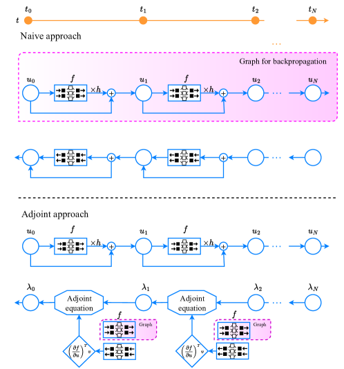
Figure 1: Schematic illustrating how the adjoint approach leads to shallower graph for backpropagation compared with the naive approach. The forward model corresponds to the Euler method.

3.2 Proposed PNODE framework

Based on the discrete adjoint method, we propose a new neural ODE framework, PNODE, that achieves reverse accuracy, memory efficiency, and flexibility at the same time. Unlike the naive approach, PNODE does not record any computational graph in the forward pass. Instead, we checkpoint the solutions at select time steps, with the stage values if multistage time integration methods such as Runge–Kutta methods are used. In the reverse pass, the checkpoints are restored and used to compute $\left(\frac{\partial\bm{f}}{\partial\bm{u}}\right)^{T}$ or the transposed Jacobian-vector product $\left(\frac{\partial\bm{f}}{\partial\bm{u}}\right)^{T}v$, where the vector $v$ is determined by the time integration algorithm. The transposed Jacobian-vector product is a required ingredient in the discrete adjoint method; it is obtained by backpropagating $\bm{f}$ with a constant memory cost $\mathcal{O}(N_{l})$, as illustrated in Figure 1. Note that the high-level discrete adjoint formula (7) can be derived for any time integration method and implemented manually, and it can be reused in different applications. Automatic derivation and implementation of the adjoint model might be possible with similar techniques used by the dolfin-adjoint project [24]. The algorithm for training PNODE is summarized in Algorithm 6.

Algorithm 1 PNODE to achieve accuracy and memory efficiency with high-level adjoint differentiation.

Forward

Solve (1) with a time-stepping algorithm (6)

Checkpoint the states and stage values for all or selective time steps

Compute the loss $\mathcal{L}$

Backward

Initialize the adjoint variables $\bm{\lambda}$ and $\bm{\mu}$ with (8)

for $n\coloneqq N-1$ to $0$ do

     Restore from the closest checkpoint, and recompute the forward pass to time $t_{n+1}$

     Compute $\bm{\lambda}_{n}$ and $\bm{\mu}_{n}$ with (7)

end for

Output the gradient $\frac{d\mathcal{L}}{d\bm{\theta}}=\mu_{0}$

The checkpointing process in PNODE provides a trade-off between storage and computational overhead. The maximum space needed for checkpointing is $(N_{t}\text{-}1)\times size\_of\_a\_checkpoint$, where a checkpoint consists of the state vector and $N_{s}$ stage vectors for one time step. In the ideal case where memory is sufficient for saving all stages, no time steps are recomputed in the backward pass. With a limited memory budget ($N_{c}<N_{t}{-}1$), the states that are not checkpointed in the forward pass can be recomputed from a nearby checkpoint. To minimize the number of recomputations, we use the binomial strategy presented in [25, 26]. The algorithm is an extension of the classic Revolve algorithm [27]. Its optimality for multistage time integration methods is proved in [25] and summarized below. We refer readers to [25, 26] for illustrations of the checkpointing procedure.

Proposition 2

[25, 26] Given $N_{c}$ allowed checkpoints in memory, the minimal number of extra forward steps (recomputations) needed for the adjoint computation of $N_{t}$ time steps is

$$\tilde{p}(N_{t},N_{c})=(t-1)\,N_{t}-\binom{N_{c}+t}{t-1}+1,$$ (10)

where $t$ is the unique integer satisfying $\binom{N_{c}+t-1}{t-1}<N_{t}\leq\binom{N_{c}+t}{t}$.

The total memory cost of PNODE thus consists of two parts: backpropogation for NN (the function $\bm{f}$) and checkpointing for the adjoint calculation. NN backpropagation requires $\mathcal{O}(N_{l})$ memory, while the memory cost of checkpointing is at most $\mathcal{O}((N_{t}\text{-}1)(N_{s}\text{+}1))$.

The computation cost of PNODE can be split into three parts: the forward computation, the reverse computation, and the recomputation overhead. The forward or reverse computation cost is $\mathcal{O}(N_{t}N_{l})$, which is common for any neural ODE approach. The recomputation cost depends on the memory budget and becomes zero when $(N_{t}\text{-}1)$ checkpoints are allowed.

3.3 Enabling implicit time integration

The application of implicit time integration is highly desired for stiff dynamical systems where explicit methods may fail because of stability constraints. Backpropagating through the implicit solver with a low-level AD tool is difficult, however, because of the complexity of the nonlinear/linear solve required at each time step and the large amount of memory needed for the resulting computational graph. By taking the function ($\bm{f}$) evaluation as a primitive operation in high-level AD, PNODE excludes the nonlinear/linear solvers from the computational graph for backpropagation. Instead, it solves an adjoint equation (a transposed linear system) to propagate the gradients. Take the backward Euler method for example. Consider a more general parameterized dynamical system in the form (common for mechanical systems)

$$\bm{\mathcal{M}}\frac{d\bm{u}}{dt}=\bm{f}(\bm{u},\bm{\theta},t)\quad\bm{u}(t_{0})=\bm{u}_{0},\quad t\in[t_{0},t_{F}],$$ (11)

where $\bm{\mathcal{M}}$ is the mass matrix (when $\bm{\mathcal{M}}$ is an identity matrix, it falls back to (1)). The backward Euler formula for solving this system is

$$\bm{\mathcal{M}}\bm{u}_{n+1}=\bm{\mathcal{M}}\bm{u}_{n}+h_{n}\bm{f}(\bm{u}_{n+1},\bm{\theta},t_{n+1}).$$ (12)

Its discrete adjoint in a simplified form (with no integral term in loss function (2)) can be written as

$$\bm{\mathcal{M}}^{T}\bm{\lambda}_{s} =\bm{\lambda}_{n+1}+h\,\left(\frac{\partial\bm{f}(\bm{u}_{n+1},\bm{\theta},t_{n+1}}{\partial\bm{u}}\right)^{T}\,\bm{\lambda}_{s},$$ (13)

$$\bm{\lambda}_{n} =\bm{\lambda}_{n+1}+h\,\left(\frac{\partial\bm{f}(\bm{u}_{n+1},\bm{\theta},t_{n+1}}{\partial\bm{u}}\right)^{T}\,\bm{\lambda}_{s},$$

$$\bm{\mu}_{n} =\bm{\mu}_{n+1}+h\,\left(\frac{\partial\bm{f}(\bm{u}_{n+1},\bm{\theta},t_{n+1}}{\partial\bm{\theta}}\right)^{T}\,\bm{\lambda}_{s}.$$

At each reverse step, (13) requires solving the transposed linear system $\bm{\mathcal{M}}^{T}-h\left(\frac{\partial\bm{f}(\bm{u}_{n+1},\bm{\theta},t_{n+1}}{\partial\bm{u}}\right)^{T}$ with respect to the adjoint variable $\bm{\lambda}_{s}$.

We solve both the linear systems in the forward pass and the transposed systems in the reverse pass with a matrix-free iterative method for efficiency. The action of the matrix or its transpose is computed by using PyTorch’s AD to backpropagate $\bm{f}$. Again, only the computational graph for $\bm{f}$ needs to be created in our approach.

3.4 Implementation

Drawing on state-of-the-art adjoint-capable ODE solvers (TSAdjoint in PETSc [28]), we implemented PNODE by interfacing PETSc to PyTorch and utilizing its discrete adjoint solvers with optimal checkpointing. As a key step, we implemented a data conversion mechanism in petsc4py, the Python bindings for PETSc, based on the DLPack standard. This enables in-place conversion between PETSc vectors and PyTorch tensors for both CPUs and GPUs and thus allows PETSc and PyTorch to access the same data seamlessly. Although PNODE can be implemented with any differentiable ODE solver such as FATODE [19] and DiffEqSensitivity.jl [29], PETSc has several favorable features that other tools lack.

Rich set of numerical integrators As a widely used time-stepping library, PETSc offers a large collection of time integration algorithms for solving ODEs, differential algebraic equations, and hybrid dynamical systems [30, 22]. It includes explicit and implicit methods, implicit-explicit methods, multirate methods with various stability properties, and adaptive time-stepping. It also provides a variety of advanced nonlinear/linear solvers that can be used in PNODE. The discrete adjoint approach proposed in Section 2.2 has been implemented for some time integrators and can be easily expanded to others [18].

Discrete adjoint solvers with matrix-free Jacobian When using the adjoint solver, we compute the transposed Jacobian-vector product through Autograd in PyTorch and supply it as a callback function to the solver, instead of building the Jacobian matrix and performing matrix-vector products, which are expensive tasks especially for dense matrices. In addition, combining low-level AD with the high-level discrete adjoint solver guarantees reverse accuracy, as explained in Section 2.4.

Optimal checkpointing for multistage methods In addition to the offline binomial checkpointing algorithms [27, 25, 26], PETSc supports more sophisticated checkpointing algorithms such as online algorithms [31] for hierarchical storage systems.

HPC-friendly linear algebra kernels PETSc has full-fledged GPU support for efficient training of neural ODEs, including multiprecision support (half, single, double, float128) and extensive parallel computing that leverages CUDA-aware MPI [32].

4 Comparison with existing methods

Table 2: Comparison between different implementations of neural ODEs for $N_{b}$ ODE blocks. The computational complexity is measured in terms of the number of function evaluations ($\bm{f}$).

	NODE cont	NODE naive	ANODE	ACA	PNODE (Ours)
Forward computation	$N_{b}N_{t}N_{s}$	$N_{b}N_{t}N_{s}$	$N_{b}N_{t}N_{s}$	$N_{b}N_{t}N_{s}$	$N_{b}N_{t}N_{s}$
Reverse computation	$N_{b}N_{t}^{B}N_{s}$	$N_{b}N_{t}N_{s}$	$N_{b}N_{t}N_{s}$	$N_{b}N_{t}N_{s}$	$N_{b}N_{t}N_{s}$
Recomputation overhead	$N_{b}N_{t}^{B}N_{s}$	$0$	$N_{b}N_{t}N_{s}$	$2N_{b}N_{t}N_{s}$	$\geq 0$
NN Backpropagation memory	$N_{l}$	$N_{b}N_{t}N_{s}N_{l}$	$N_{t}N_{s}N_{l}$	$N_{s}N_{l}$	$N_{l}$
Adjoint checkpointing memory	–	–	$N_{b}$	$N_{b}N_{t}$	$\leq N_{b}(N_{t}\text{-}1)(N_{s}\text{+}1)$
Reverse-accuracy	$\color[rgb]{1,0,0}\times$	$\color[rgb]{0,0,1}\checkmark$	$\color[rgb]{0,0,1}\checkmark$	$\color[rgb]{0,0,1}\checkmark$	$\color[rgb]{0,0,1}\checkmark$
Implicit time-stepping support	$\color[rgb]{1,0,0}\times$	$\color[rgb]{1,0,0}\times$	$\color[rgb]{1,0,0}\times$	$\color[rgb]{1,0,0}\times$	$\color[rgb]{0,0,1}\checkmark$

A summary comparing PNODE with representative implementations of neural ODEs is given in Table 2. The memory and computation costs are given for one ODE block. When multiple ODE blocks are considered, the costs need to be multiplied by a factor of $N_{b}$ except for ANODE. For simplicity, we assume that the number of reverse time steps in the continuous adjoint method is also $N_{t}$ and do not consider rejected time steps. Note that the rejected time steps have no influence on the computational cost and the memory cost of PNODE because the adjoint calculation in the reverse pass involves only accepted time steps [25].

NODE cont: the original implementation in [4] with continuous adjoint The vanilla neural ODE [4] avoids recording everything by solving the ODE backward in time to obtain the intermediate solutions needed when solving the continuous adjoint equation. Therefore, it requires a constant memory cost $\mathcal{O}(N_{l})$ to backpropagate $\bm{f}$. The backward ODE solve requires a recomputation cost of $\mathcal{O}(N_{t}^{B}N_{s})$.

NODE naive: a variant of the original implementation in [4] This is a naive method that backpropagates the ODE solvers with low-level AD and has the deepest computational graph, but it has no recomputational overhead.

ANODE: a framework with discrete adjoint and checkpointing method [11] The checkpointing method for ANODE has the same memory cost $\mathcal{O}(N_{t})$ as NODE naive when a single ODE block is considered. For multiple ODE blocks, ANODE saves only the initial states for each block and recomputes the forward pass before the backpropagation for each block; consequently, the memory cost for checkpointing is $\mathcal{O}(N_{b})$, where $N_{b}$ is the number of ODE blocks, and the backpropagation requires $\mathcal{O}(N_{t}N_{s}N_{l})$ memory, which is independent of $N_{b}$. Each ODE block needs to be recomputed in the backward pass, so the total recomputation cost is $\mathcal{O}(N_{t}N_{s})$. A generalization of ANODE has been implemented in a Julia library [33].

ACA: the adaptive checkpoint adjoint (ACA) method [13] ACA is similar to ANODE but uses a slightly different checkpointing strategy. ACA checkpoints the state at each time step, thus consuming $\mathcal{O}(N_{t})$ memory for checkpointing. To save memory, ACA deletes redundant computational graphs for rejected time steps when searching for the optimal step size. Although it is shown in [13] that ACA uses the continuous adjoint approach, the actual implementation of ACA applies backpropagation with low-level AD to each time step, so it requires $\mathcal{O}(N_{s}N_{l})$ memory. In the backward pass, ACA first performs an additional forward pass to save the checkpoints and then recomputes each time step to generate the local computational graph, resulting in a total recomputation cost of $\mathcal{O}(2N_{t}N_{s})$.

5 Experimental Results

In this section we test the performance of PNODE and compare it with existing neural ODE methods on two distinct benchmark tasks: image classification and continuous normalizing flows (CNF). We then demonstrate the application of PNODE to learning stiff dynamics. All the experiments are conducted on an NVIDIA Tesla V100 GPU with a memory capacity of 32 GB. When testing PNODE, unless specified otherwise, we assume $N_{c}\geq N_{t}$ and checkpoint all the intermediate solutions and stage values for the best speed. Note that this approach leads to no recomputation, thus giving the best speed but also the worst-case memory cost for PNODE.

Existing frameworks may support only a subset of the time integration schemes used in our experiments. For a comprehensive and fair evaluation and comparison, we have added the same time integration schemes in all frameworks if they were not originally implemented. In the benchmark tests, we focused on fixed step schemes instead of adaptive step schemes because error estimation and adaptive strategies can be vastly different across different frameworks, making a fair comparison difficult, especially when investigating memory consumption, which is sensitive to the number of time steps. The results for fixed step schemes can reflect the fundamental differences among the neural ODE methods and indicate the expected performance of these methods for adaptive step schemes.

5.1 Image classification

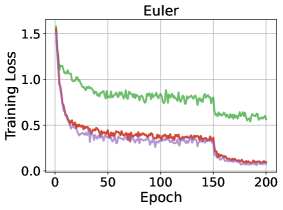
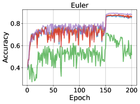
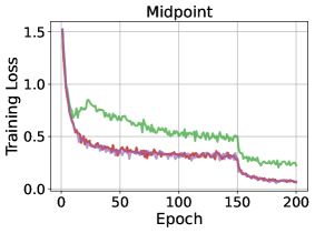
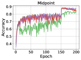
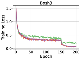
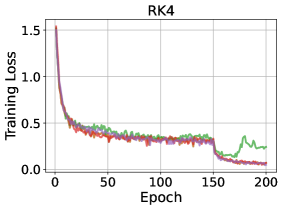
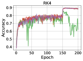
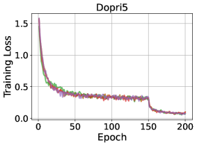
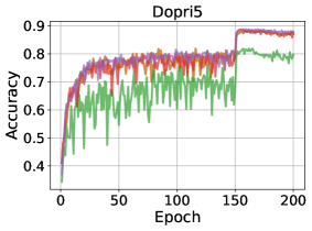
Figure 2: Training and testing performance of SqueezeNext on CIFAR10 using various schemes with one time step. The inaccuracy in the gradient calculated via continuous adjoint causes a significant gap in performance between discrete adjoint and continuous adjoint.

Chen et al. [4] showed that replacing residual blocks with ODE blocks yields good accuracy and parameter efficiency on the MNIST dataset from [34]. However, the effect of the accuracy of the gradients cannot be determined easily with this simple dataset. Here we experiment on the more complex CIFAR-10 dataset from [35] using a SqueezeNext network introduced by [36], where every nontransition block is replaced with a neural ODE block. We use $4$ ODE blocks of different dimensions with $199,800$ trainable parameters in total.

Accuracy

We train the same neural ODE structure using one time step while varying the time integration method. The results are displayed in Figure 2. The ReLU activation in this model results in irreversible dynamics and inaccurate gradient calculation for the vanilla neural ODE [4], leading to divergent training with the Euler method and the RK4 method and to suboptimal accuracy. PNODE and other neural ODE methods converge to higher accuracy because of the reverse accuracy guaranteed by the discrete adjoint method and automatic differentiation. With the low-accuracy methods (Euler and Midpoint), PNODE achieves the highest accuracy among all the methods tested.

Memory/time efficiency

We perform a systematic comparison of the efficiency and memory cost for different methods by varying $N_{t}$. In all the experiments, we measure the total amount of consumed GPU memory. For PNODE, we include an additional variant (denoted by PNODE2) that saves only the ODE solution at each time step. This leads to $N_{t}\text{-}1$ recomputations in the reverse pass and a memory cost of $N_{b}(N_{t}\text{-}1)$ for adjoint checkpointing. Thus PNODE2 has almost the same total memory cost as ACA has. As shown in Figure 3, PNODE significantly outperforms all the other methods in terms of per-epoch training time. When using Dopri5, PNODE is three times faster than ANODE, $2.3$ times faster than ACA, and two times faster than the vanilla neural ODE. Similar speedups can be observed for other time integration methods. Among all reverse-accurate methods, PNODE has the slowest memory growth as the number of time steps increases. For example, using Dopri5 with $11$ time steps, the memory consumption of PNODE is approximately $71\%$ less than NODE naive and $55\%$ less than ANODE. Compared with PNODE, PNODE2 reduces the memory cost by up to $42\%$ with a slight increase in training time. PNODE2 has a similar memory cost but much faster training speed than ACA, which agrees with the theoretical analysis shown in Table 2. Note that the CUDA runtime allocates $\sim 0.4$ GB memory for PNODE, and it is included in all the PNODE results presented in this paper. This overhead is inevitable for loading any library that contains CUDA kernels.

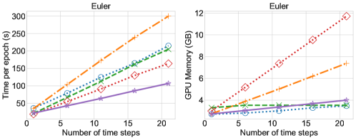
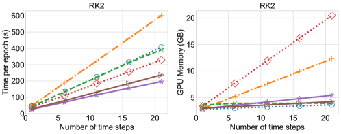
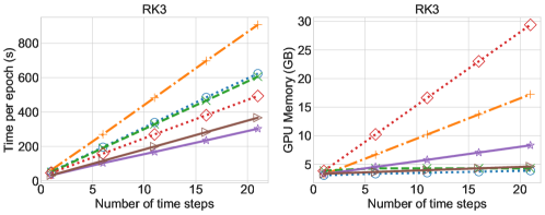
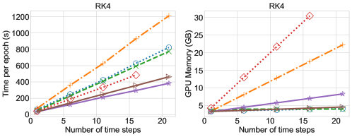
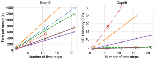
Figure 3: GPU memory usage and time per epoch of different implementations as functions of the number of time steps ($N_{t}$) for various schemes.

5.2 Continuous normalizing flow for density estimation

We select three datasets—POWER, MINIBOONE, and BSDS3000—that are respectively 6-, 43-, and 63-dimensional tabular datasets commonly used in CNF [37]. The FFJORD [5] approach is used to transform a multivariate Gaussian distribution to the target distributions for all three datasets.

We adopt the tuned architecture and hyperparameters (e.g., learning rates, number of hidden layers, and number of flow steps) from [5]. We vary the number of steps for different time integration methods only for stability considerations. On all three datasets, all the methods that converge yield comparable testing losses, but all the reverse-accurate methods converge much faster than NODE cont because of more accurate gradient estimates. On BSDS300, NODE cont failed to converge after 14 days of training and was terminated prematurely. Similar observations were reported in [12].

The performance statistics including the number of function evaluations per iteration, the training time per iteration, and the maximum GPU memory usage are shown in Tables 7, 3, 4, 5 and 6. NFE-F and NFE-B are the number of function evaluations in the forward pass and backward pass, respectively. NFE-B for PNODE and NODE cont reflects the cost of the transposed Jacobian-vector products, while NFE-B for other methods reflects the cost for recomputing the time steps in the backward pass. The observed results agree with our theoretical analysis in Table 2.

Excluding the $0.4$ GB constant overhead, PNODE has the lowest memory consumption among all reverse-accurate methods, and it consistently outperforms ACA and ANODE in terms of training time for all three datasets. When using the Dopri5 scheme that is commonly used in neural ODEs, PNODE is $28.7\%$ faster and consumes $68.2\%$ less memory than does ACA for BSDS300. The advantage becomes more evident for high-order schemes that have more stages. The reason is that the computational graph for automatic differentiation grows deeper as the number of stages increases.

NODE naive and ANODE run out of GPU memory for BSDS300. But when memory is sufficient, NODE naive is the fastest, as expected. For MINIBOONE, the difference in memory consumption is marginal for all methods because of a number of factors such as small batch size ($1000$), small number of steps ($4$), and small neural network.

Table 3: Performance statistics for the Euler scheme. Missing values are due to out-of-memory errors.

Dataset	Framework	Integration method	NFE-F	NFE-B	Time per iteration (s)	GPU Mem (GB)
POWER	NODE naive	Euler, $N_{t}$=50	250	0	0.760	11.648
	NODE cont		250	250	1.101	1.680
	ANODE		250	250	1.297	3.624
	ACA		250	505	1.382	1.735
	PNODE		250	250	1.117	2.104
MINIBOONE	NODE naive	Euler, $N_{t}$=20	20	0	0.071	2.481
	NODE cont		20	20	0.094	1.716
	ANODE		20	20	0.108	2.500
	ACA		20	41	0.102	1.762
	PNODE		20	20	0.099	2.085
BSDS300	NODE naive	Euler, $N_{t}$=100	–	–	–	–
	NODE cont		200	200	13.409	3.826
	ANODE		–	–	–	–
	ACA		200	402	17.191	5.564
	PNODE		200	200	13.541	4.920

Table 4: Performance statistics for the Midpoint scheme.

Dataset	Framework	Integration method	NFE-F	NFE-B	Time per iteration (s)	GPU Mem (GB)
POWER	NODE naive	Midpoint, $N_{t}$=40	400	0	1.368	17.659
	NODE cont		400	400	1.780	1.680
	ANODE		400	400	1.975	4.822
	ACA		400	805	2.109	1.819
	PNODE		400	400	1.883	2.152
MINIBOONE	NODE naive	Midpoint, $N_{t}$=16	32	0	0.104	2.991
	NODE cont		32	32	0.134	1.737
	ANODE		32	32	0.167	3.012
	ACA		32	65	0.145	1.846
	PNODE		32	32	0.137	2.087
BSDS300	NODE naive	Midpoint, $N_{t}$=80	–	–	–	–
	NODE cont		320	320	21.404	3.826
	ANODE		–	–	–	–
	ACA		320	642	24.977	7.525
	PNODE		320	320	21.651	5.388

Table 5: Performance statistics for the Bosh3 scheme.

Dataset	Framework	Integration method	NFE-F	NFE-B	Time per iteration (s)	GPU Mem (GB)
POWER	NODE naive	Bosh3, $N_{t}$=30	465	0	1.532	20.282
	NODE cont		465	465	3.058	6.555
	ANODE		450	450	2.593	10.106
	ACA		450	905	2.632	6.771
	PNODE		455	450	2.084	2.217
MINIBOONE	NODE naive	Bosh3, $N_{t}$=12	32	0	0.1041	2.991
	NODE cont		39	39	0.164	1.737
	ANODE		36	36	0.187	3.182
	ACA		36	73	0.219	1.930
	PNODE		37	36	0.153	2.091
BSDS300	NODE naive	Bosh3, $N_{t}$=60	–	–	–	–
	NODE cont		366	366	22.905	3.878
	ANODE		–	–	–	–
	ACA		360	722	31.001	9.821
	PNODE		362	360	24.439	6.145

Table 6: Performance statistics for the RK4 scheme.

Dataset	Framework	Integration method	NFE-F	NFE-B	Time per iteration (s)	GPU Mem (GB)
POWER	NODE naive	RK4, $N_{t}$=20	400	0	1.615	22.529
	NODE cont		400	400	2.291	6.553
	ANODE		400	400	2.345	9.697
	ACA		400	805	2.365	6.834
	PNODE		400	400	1.765	2.156
MINIBOONE	NODE naive	RK4, $N_{t}$=8	32	0	0.110	2.991
	NODE cont		32	32	0.131	1.737
	ANODE		32	32	0.168	3.012
	ACA		32	65	0.200	2.016
	PNODE		32	32	0.135	2.089
BSDS300	NODE naive	RK4, $N_{t}$=40	–	–	–	–
	NODE cont		320	320	21.097	3.878
	ANODE		–	–	–	–
	ACA		320	642	27.035	12.053
	PNODE		320	320	21.681	5.422

Table 7: Performance statistics for the Dopri5 scheme.

Dataset	Framework	Integration method	NFE-F	NFE-B	Time per iteration (s)	GPU Mem (GB)
POWER	NODE naive	Dopri5, $N_{t}$=10	300	0	0.976	13.653
	NODE cont		300	300	1.357	1.687
	ANODE		300	300	1.524	4.035
	ACA		300	605	1.816	2.131
	PNODE		305	300	1.329	2.150
MINIBOONE	NODE naive	Dopri5, $N_{t}$=4	24	0	0.074	2.653
	NODE cont		24	24	0.120	1.758
	ANODE		24	24	0.131	2.672
	ACA		24	49	0.143	2.184
	PNODE		25	24	0.105	2.089
BSDS300	NODE naive	Dopri5, $N_{t}$=20	–	–	–	–
	NODE cont		240	240	16.175	3.983
	ANODE		–	–	–	–
	ACA		240	482	21.003	16.667
	PNODE		242	240	16.314	5.304

5.3 Learning stiff dynamics

Stiff dynamical systems are characterized by widely separated time scales, which pose computational difficulties for explicit time integration methods. Several researchers [38, 39, 40] have recognized that learning stiff dynamics from time-series data is also challenging for data-driven approaches such as neural ODEs. The reasons are twofold. First, the computational difficulties in solving stiff ODEs remain in neural ODEs. Second, stiffness could lead to ill-conditioned gradients in classical neural ODEs. Kim et al. [39] proposed applying scaling to the differential equations and loss functions to mitigate stiffness. In this section we apply feature scaling to the input data and then use an implicit method for training the neural ODEs. We demonstrate the success of our approach with a well-known stiff chemical reaction system and illuminate the benefits of using implicit solvers, which are equipped with discrete adjoint capabilities and efficient nonlinear and linear solvers, uniquely enabled through PNODE.

The system we consider is governed by Robertson’s equations:

$$\frac{du_{1}}{dt} =-k_{1}u_{1}+k_{3}u_{2}u_{3},$$ (14)

$$\frac{du_{2}}{dt} =k_{1}u_{1}-k_{2}u_{2}^{2}-k_{3}u_{2}u_{3},$$

$$\frac{du_{3}}{dt} =k_{2}u_{2}^{2},$$

where $u_{1},u_{2},u_{3}$ are the concentrations of three species and $k_{1}=0.04,k_{2}=3\times 10^{7},k_{3}=10^{4}$ are reaction rate constants. We train a neural ODE in form 1 with the right-hand side function approximated by a NN. The loss function is defined as the discrepancy between the observed data and the prediction by the ML model

$$\mathcal{L}=\text{MAE}(u^{\text{ob}}(t),u^{\text{pred}}(t)),$$ (15)

where MAE is the mean absolute error. The NN has five hidden layers with an activation function of GELU as used in [39].

The training data are generated by solving (14) with the initial conditions of $[u_{1},u_{2},u_{3}]=[1,0,0]$ over a time span of $[10^{-5},100]$ and sampling $40$ data points equally spaced in a logarithm scale. We train the neural ODE for $10,000$ epochs on a GPU using the AdamW optimizer with an initial learning rate of $0.005$.

5.3.1 Data preprocessing

Since the three species have widely varying concentrations (5 orders of magnitude), their contributions to the loss function are not proportionate, thus leading to slow convergence in training. Figure 4(c) shows the results learned by using the raw data after $10,000$ epochs’ training. The predictions for the first and third species match the ground truth well; however, the second species shows a noticeable discrepancy. To remedy this issue, we apply the standard min-max normalization

$$u^{\prime}=\frac{u-\min(u)}{\max(u)-\min(u)}$$ (16)

to scale the input data to the range $[0,1]$.

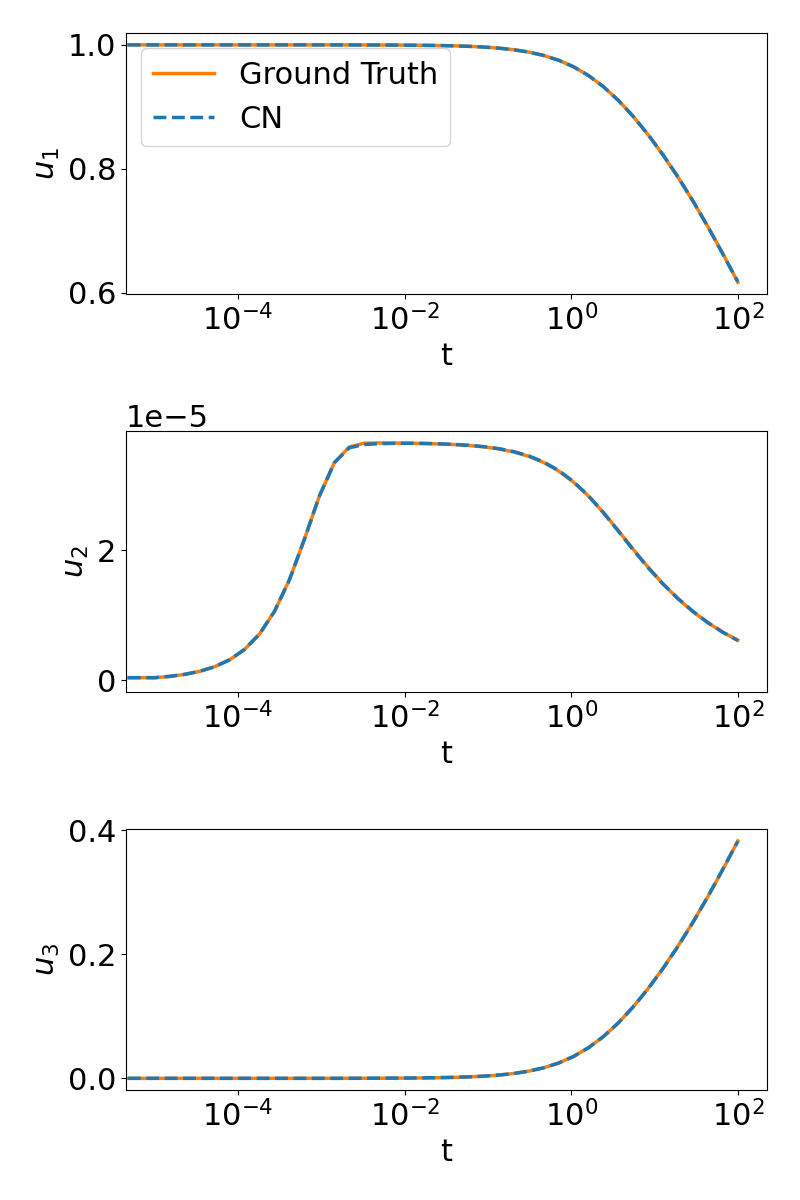
(a) Implicit method

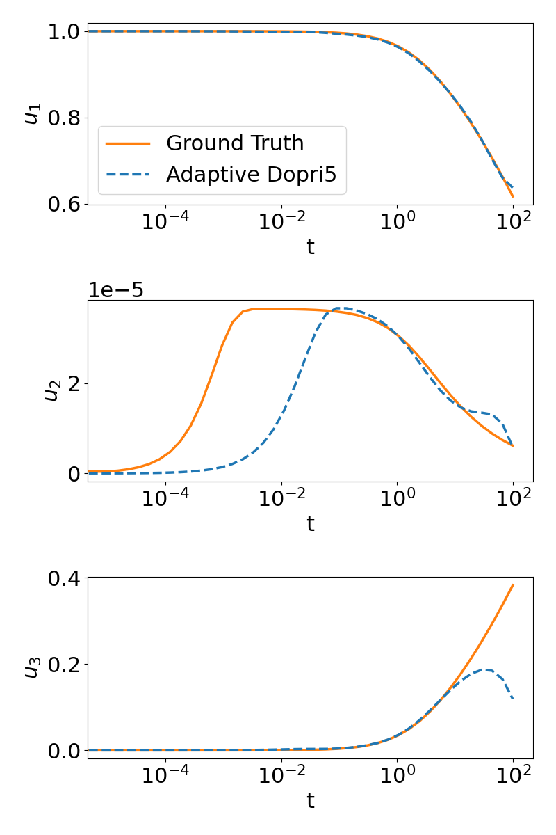
(b) Explicit method

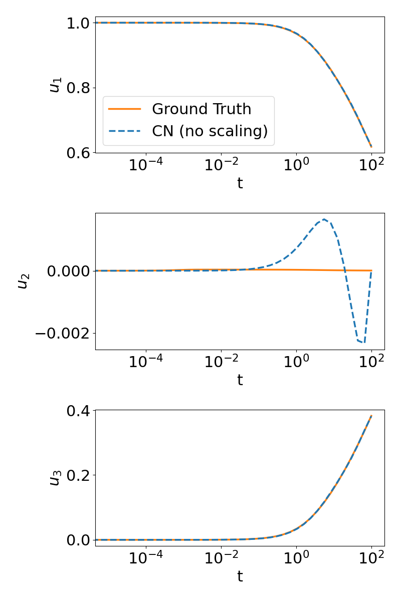
(c) Implicit method (no scaling)

Figure 4: Ground truth of Robertson’s equations and the predictions of the neural ODE models with different training methods.

5.3.2 Implicit versus explicit

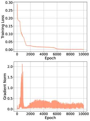
(a) CN

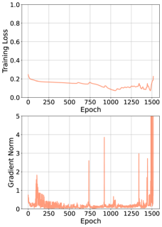
(b) Dopri5

Figure 5: Training results on Robertson’s equations with the Crank–Nicolson method (left) and with the Dopri5 method (right). Training loss is plotted on the top, and gradient norm is plotted on the bottom. The gradients for Dopri5 explode after about 1,500 epochs.

PNODE enables us to use an implicit method to integrate the forward model and use its discrete adjoint to compute the gradients for training. Here, we demonstrate the advantage of implicit methods by comparing them with the adaptive explicit methods that are widely used in existing neural ODE frameworks because of their efficiency and ease of implementation. For implicit methods, we use the Crank–Nicolson (CN) scheme. The nonlinear systems arising at each time step are solved with a Newton method, and the linear systems are solved with a matrix-free GMRES method [41]. For explicit methods we use the adaptive Dopri5 method with tolerances $abstol=reltol=10^{-6}$. As shown in Figure 5, PNODE with CN can learn the dynamics perfectly, while Dopri5 fails to match the ground truth. This result is expected because of the limitations of explicit methods in handling stiff systems. Figure 5 shows that when using Dorpi5, the gradient explodes, preventing the convergence of the training loss.

5.3.3 Computation cost

The training costs for Dopri5 and CN are given in Table 8. We can see that training with CN is slightly faster than training with Dopri5 for the Robertson’s equations. Note that function evaluations are required not only for the time integration but also for Autograd to generate the Jacobian-vector product and the transposed Jacobian-vector product, which are needed in the adjoint calculation. In principle, explicit methods have lower per-step cost than implicit methods have because they do not require solving linear systems. In our case, however, they require a large number of steps according to Table 8. Initially, the training model is not stiff, requiring relatively few time steps when integrating the neural ODE. As the training model approaches the ground truth, however, the stiffness increases, causing the number of time steps to increase as well.

Table 8: Computation cost comparison between Dopri5 and CN.

Integration method	Average NFE-F	Average NFE-B	Average time per iteration (s)
CN	505	136	0.709
Dopri5	805	805	0.778

6 Conclusion

In this work we propose PNODE, a framework for neural ODEs based on high-level discrete adjoint methods with checkpointing. We show that the discrete adjoints derived from a time integration scheme can be cast as a high-level abstraction of automatic differentiation and produce gradients exact to machine precision. Adopting this approach, one can avoid backpropagating through an ODE solver or a time integration procedure by directly using ML platforms such as TensorFlow and PyTorch and can minimize the depth of the computational graph for NN backpropagation, while guaranteeing reverse accuracy. With high-level adjoint differentiation and the checkpointing technique, we successfully reduce the memory cost of neural ODEs to $\mathcal{O}(N_{t}N_{s})+\mathcal{O}(N_{l})$ when checkpointing all intermediate states (including ODE solutions and stage vectors) and $\mathcal{O}(N_{t})+\mathcal{O}(N_{l})$ when checkpointing solutions only, whereas a naive automatic differentiation approach requires a memory cost of $\mathcal{O}(N_{t}N_{s}N_{l})$. Extensive numerical experiments on image classification and continuous normalizing flow problems show that PNODE achieves the best memory efficiency and training speed among the existing neural ODEs that are reverse-accurate. Furthermore, our high-level adjoint method not only allows a balance between memory and computational costs but also offers more flexibility in the solver design than traditional neural ODEs have. We demonstrate that PNODE enables the application of implicit integration methods, which offers more possibilities for stabilizing the training of stiff dynamical systems and building implicit deep learning models [42]. We have made PNODE freely available and believe that accelerated memory-efficient neural ODEs will benefit a broad range of artificial intelligence applications, especially for scientific machine learning tasks such as the discovery of unknown physics.

References

- [1] Y. Lu, A. Zhong, Q. Li, and B. Dong, “Beyond finite layer neural networks: Bridging deep architectures and numerical differential equations,” in Proceedings of the 35th International Conference on Machine Learning, vol. 80. PMLR, 10–15 Jul 2018, pp. 3276–3285.
- [2] E. Haber and L. Ruthotto, “Stable architectures for deep neural networks,” Inverse Problems, vol. 34, no. 1, p. 014004, 12 2017.
- [3] L. Ruthotto and E. Haber, “Deep neural networks motivated by partial differential equations,” Journal of Mathematical Imaging and Vision, vol. 62, no. 3, pp. 352–364, 2020.
- [4] R. T. Q. Chen, Y. Rubanova, J. Bettencourt, and D. K. Duvenaud, “Neural ordinary differential equations,” in Advances in Neural Information Processing Systems, vol. 31. Curran Associates, Inc., 2018.
- [5] W. Grathwohl, R. T. Q. Chen, J. Bettencourt, and D. Duvenaud, “Scalable reversible generative models with free-form continuous dynamics,” in International Conference on Learning Representations, 2019.
- [6] Y. Rubanova, R. T. Q. Chen, and D. K. Duvenaud, “Latent ordinary differential equations for irregularly-sampled time series,” in Advances in Neural Information Processing Systems, vol. 32. Curran Associates, Inc., 2019.
- [7] S. Greydanus Google Brain, M. Dzamba PetCube, and J. Yosinski, “Hamiltonian neural networks,” in Advances in Neural Information Processing Systems, vol. 32, 2019.
- [8] I. Ayed, E. de Bézenac, A. Pajot, J. Brajard, and P. Gallinari, “Learning dynamical systems from partial observations,” arXiv preprint arXiv:1902.11136, 2019.
- [9] E. Dupont, A. Doucet, and Y. W. Teh, “Augmented neural ODEs,” in Advances in Neural Information Processing Systems, vol. 32. Curran Associates, Inc., 2019.
- [10] J. Jia and A. R. Benson, “Neural jump stochastic differential equations,” in Advances in Neural Information Processing Systems, vol. 32. Curran Associates, Inc., 2019.
- [11] A. Gholaminejad, K. Keutzer, and G. Biros, “ANODE: Unconditionally accurate memory-efficient gradients for neural ODEs,” in Proceedings of the Twenty-Eighth International Joint Conference on Artificial Intelligence, IJCAI-19. International Joint Conferences on Artificial Intelligence Organization, 7 2019, pp. 730–736.
- [12] D. Onken and L. Ruthotto, “Discretize-optimize vs. optimize-discretize for time-series regression and continuous normalizing flows,” arXiv preprint arXiv:2005.13420, 2020.
- [13] J. Zhuang, N. Dvornek, X. Li, S. Tatikonda, X. Papademetris, and J. Duncan, “Adaptive checkpoint adjoint method for gradient estimation in neural ODE,” in Proceedings of the 37th International Conference on Machine Learning, vol. 119, 2020, pp. 11 639–11 649.
- [14] T. Zhang, Z. Yao, A. Gholami, J. E. Gonzalez, K. Keutzer, M. W. Mahoney, and G. Biros, “ANODEV2: A coupled neural ODE framework,” in Advances in Neural Information Processing Systems, vol. 32. Curran Associates, Inc., 2019.
- [15] J. Zhuang, N. C. Dvornek, S. Tatikond, and J. S. Duncan, “MALI: A memory efficient and reverse accurate integrator for neural ODEs,” in International Conference on Learning Representations, 2021.
- [16] T. Beck, “Automatic differentiation of iterative processes,” Journal of Computational and Applied Mathematics, vol. 50, pp. 109–118, 1994.
- [17] C. Finlay, J.-H. Jacobsen, L. Nurbekyan, and A. Oberman, “How to train your neural ODE: the world of Jacobian and kinetic regularization,” in Proceedings of the 37th International Conference on Machine Learning, vol. 119. PMLR, 13–18 July 2020, pp. 3154–3164.
- [18] H. Zhang, E. M. Constantinescu, and B. F. Smith, “PETSc TSAdjoint: a discrete adjoint ODE solver for first-order and second-order sensitivity analysis,” SIAM Journal on Scientific Computing, vol. 44, no. 1, pp. C1–C24, 2022.
- [19] H. Zhang and A. Sandu, “FATODE: a library for forward, adjoint, and tangent linear integration of ODEs,” SIAM Journal on Scientific Computing, vol. 36, no. 5, pp. C504–C523, 2014.
- [20] E. J. Nielsen and W. L. Kleb, “Efficient construction of discrete adjoint operators on unstructured grids using complex variables,” AIAA Journal, vol. 44, no. 4, pp. 827–836, 2006.
- [21] E. J. Nielsen and B. Diskin, “Discrete adjoint-based design for unsteady turbulent flows on dynamic overset unstructured grids,” AIAA Journal, vol. 51, no. 6, pp. 1355–1373, 2013.
- [22] H. Zhang, S. Abhyankar, E. Constantinescu, and M. Anitescu, “Discrete adjoint sensitivity analysis of hybrid dynamical systems with switching,” IEEE Transactions on Circuits and Systems I: Regular Papers, vol. 64, no. 5, pp. 1247–1259, 2017.
- [23] J. Nocedal and S. J. Wright, Numerical Optimization, 2nd ed. New York, NY, USA: Springer, 2006.
- [24] P. E. Farrell, D. A. Ham, S. F. Funke, and M. E. Rognes, “Automated derivation of the adjoint of high-level transient finite element programs,” SIAM Journal on Scientific Computing, vol. 35, no. 4, pp. 369–393, 2013.
- [25] H. Zhang and E. M. Constantinescu, “Revolve-based adjoint checkpointing for multistage time integration,” in International Conference on Computational Science, (online), in main track, 2021.
- [26] H. Zhang and E. Constantinescu, “Optimal checkpointing for adjoint multistage time-stepping schemes,” arXiv preprint arXiv:2106.13879, 2022.
- [27] A. Griewank and A. Walther, “Algorithm 799: Revolve: an implementation of checkpointing for the reverse or adjoint mode of computational differentiation,” ACM Transaction on Mathematical Software, vol. 26, no. 1, p. 19–45, Mar. 2000.
- [28] S. Balay, S. Abhyankar, M. F. Adams, J. Brown, P. Brune, K. Buschelman, L. Dalcin, A. Dener, V. Eijkhout, W. D. Gropp, D. Karpeyev, D. Kaushik, M. G. Knepley, D. A. May, L. C. McInnes, R. T. Mills, T. Munson, K. Rupp, P. Sanan, B. F. Smith, S. Zampini, H. Zhang, and H. Zhang, “PETSc users manual,” Argonne National Laboratory, Tech. Rep. ANL-95/11 - Revision 3.14, 2020.
- [29] C. Rackauckas and Q. Nie, “DifferentialEquations.jl -– a performant and feature-rich ecosystem for solving differential equations in Julia,” The Journal of Open Research Software, vol. 5, no. 1, 2017.
- [30] S. Abhyankar, J. Brown, E. M. Constantinescu, D. Ghosh, B. F. Smith, and H. Zhang, “PETSc/TS: a modern scalable ODE/DAE solver library,” arXiv preprint arXiv:1806.01437, 2018.
- [31] P. Stumm and A. Walther, “New algorithms for optimal online checkpointing,” SIAM Journal on Scientific Computing, vol. 32, no. 2, pp. 836–854, 2010.
- [32] R. T. Mills, M. F. Adams, S. Balay, J. Brown, A. Dener, M. Knepley, S. E. Kruger, H. Morgan, T. Munson, K. Rupp, B. F. Smith, S. Zampini, H. Zhang, and J. Zhang, “Toward performance-portable PETSc for GPU-based exascale systems,” Parallel Computing, vol. 108, p. 102831, 2021.
- [33] C. Rackauckas, Y. Ma, J. Martensen, C. Warner, K. Zubov, R. Supekar, D. Skinner, and A. Ramadhan, “Universal differential equations for scientific machine learning,” arXiv preprint arXiv:2001.04385, 2020.
- [34] Y. Lecun, L. Bottou, Y. Bengio, and P. Haffner, “Gradient-based learning applied to document recognition,” Proceedings of the IEEE, vol. 86, no. 11, pp. 2278–2324, 1998.
- [35] A. Krizhevsky, “Learning multiple layers of features from tiny images,” University of Toronto, 05 2012.
- [36] A. Gholami, K. Kwon, B. Wu, Z. Tai, X. Yue, P. Jin, S. Zhao, and K. Keutzer, “SqueezeNext: Hardware-aware neural network design,” in Proceedings of the IEEE Conference on Computer Vision and Pattern Recognition (CVPR) Workshops, June 2018.
- [37] G. Papamakarios, T. Pavlakou, and I. Murray, “Masked autoregressive flow for density estimation,” in Advances in Neural Information Processing Systems, vol. 30, 2017.
- [38] A. Ghosh, H. Behl, E. Dupont, P. Torr, and V. Namboodiri, “STEER: Simple temporal regularization for neural ODE,” in Advances in Neural Information Processing Systems, vol. 33. Curran Associates, Inc., 2020, pp. 14 831–14 843.
- [39] S. Kim, W. Ji, S. Deng, Y. Ma, and C. Rackauckas, “Stiff neural ordinary differential equations,” Chaos: An Interdisciplinary Journal of Nonlinear Science, vol. 31, no. 9, p. 093122, 2021.
- [40] S. Liang, Z. Huang, and H. Zhang, “Stiffness-aware neural network for learning Hamiltonian systems,” in International Conference on Learning Representations, 2022.
- [41] Y. Saad and M. H. Schultz, “GMRES: A generalized minimal residual algorithm for solving nonsymmetric linear systems,” SIAM Journal on Scientific and Statistical Computing, vol. 7, no. 3, pp. 856–869, 1986.
- [42] L. El Ghaoui, F. Gu, B. Travacca, A. Askari, and A. Tsai, “Implicit deep learning,” SIAM Journal on Mathematics of Data Science, vol. 3, no. 3, pp. 930–958, 2021.