Improving Quantum Computation
by Optimized Qubit Routing

Abstract

In this work we propose a high-quality decomposition approach for qubit routing by swap insertion. This optimization problem arises in the context of compiling quantum algorithms formulated in the circuit model of computation onto specific quantum hardware. Our approach decomposes the routing problem into an allocation subproblem and a set of token swapping problems. This allows us to tackle the allocation part and the token swapping part separately. Extracting the allocation part from the qubit routing model of Nannicini et al. ([18]), we formulate the allocation subproblem as a binary linear program. Herein, we employ a cost function that is a lower bound on the overall routing problem objective. We strengthen the linear relaxation by novel valid inequalities. For the token swapping part we develop an exact branch-and-bound algorithm. In this context, we improve upon known lower bounds on the token swapping problem. Furthermore, we enhance an existing approximation algorithm which runs much faster than the exact approach and typically is able to determine solutions close to the optimum. We present numerical results for the fully integrated allocation and token swapping problem. Obtained solutions may not be globally optimal due to the decomposition and the usage of an approximation algorithm. However, the solutions are obtained fast and are typically close to optimal. In addition, there is a significant reduction in the number of artificial gates and output circuit depth when compared to various state-of-the-art heuristics. Reducing these figures is crucial for minimizing noise when running quantum algorithms on near-term hardware. As a consequence, using the novel decomposition approach leads to compiled algorithms with improved quality. Indeed, when compiled with the novel routing procedure and executed on real hardware, our experimental results for quantum approximate optimization algorithms show an significant increase in solution quality in comparison to standard routing methods.
Keywords: Combinatorial Optimization, Integer Programming, Approximation Algorithms, Quantum Compilation

1 Introduction

Qubit routing by swap insertion is a subroutine in the process of compiling quantum algorithms onto specific hardware. Quantum algorithms are usually formulated in the circuit model of quantum computation, see e.g. [19] for an introduction. Such a circuit consists of wires representing qubits as well as gates representing operations applied to subsets of qubits. We refer to the qubits in the circuit as logical qubits, in contrast to the physical qubits in quantum hardware. Furthermore, we assume that the circuit only contains gates acting on at most two qubits, i.e. single and two-qubit gates (also known as “$\mathrm{SU}(4)$ circuits”). This might already be the case for the input circuit to be compiled; otherwise this can be achieved using the Solovay-Kitaev Theorem, see e.g. [19, pp. 188–202]. In the circuit model, gates may be applied on any pair of logical qubits. However, this is not the case in many currently available quantum processors. Here, two-qubit gates can only be applied on specific pairs of physical qubits defined by the hardware connectivity graph. Now the task is to choose an initial allocation of logical qubits in the quantum circuit to physical qubits in the hardware graph such that for each two-qubit gate the corresponding logical qubits are located at neighbouring physical qubits. The example in Fig. 1 shows that this is not always possible directly.

(a)

(b)

Figure 1: Example for a quantum circuit (a) consisting of four logical qubits as well as single and two-qubit gates. In the context of this work, the meaning of the gates is irrelevant. Only the subset of qubits involved in a gate matters. The circuit is not compatible with the hardware connectivity graph shown in (b).

In such a case, it is necessary to insert additional swap gates into the algorithm. They effectively swap the positions of two logical qubits in the hardware graph. The result is an $\mathrm{SU}(4)$ circuit meeting the connectivity restrictions which is equivalent to the original one when taking into account the permutation resulting from initial allocation and swap gates. A simple example for this procedure is shown in Figure 2.

Figure 2: Example for routing by swap insertion. The given circuit is equivalent to the quantum circuit from Figure 1a and fulfills the hardware connectivity from Figure 1b. The equivalence holds under the initial allocation of logical qubits $\{q_{0},q_{1},q_{2},q_{3}\}$ to physical qubits $\{0,1,2,3\}$ given by $q_{0}\mapsto 3,q_{1}\mapsto 2,q_{2}\mapsto 1,q_{3}\mapsto 0$. After the first swap the allocation changes to $q_{0}\mapsto 3,q_{1}\mapsto 2,q_{2}\mapsto 0,q_{3}\mapsto 1$, and after the second swap to $q_{0}\mapsto 3,q_{1}\mapsto 2,q_{2}\mapsto 1,q_{3}\mapsto 0$.

When solving the routing by swap insertion problem, two possible objective functions arise naturally: either one aims to minimize the execution time on the quantum processor, which can be achieved by minimizing the output circuit depth, or one can minimize the total gate number to be executed, which amounts to minimizing the number of swap gates added. Intuitively, both objectives are correlated. However, it is easy to construct examples where optimal-depth solutions are suboptimal in terms of gate count and vice versa. For an experimental study of the influence of depth and gate count on the performance of quantum algorithms, we refer to [18] and [11].

Existing methods for qubit routing.

Many compilation procedures based on routing by swap insertion have been developed so far. Some of them may be classified by their local working principle: they define an initial mapping of logical to physical qubits, iterate through the circuit in temporal order and change the allocation by adding swaps when gates are encountered which cannot be applied in the current allocation. Of course, this general principle allows for many different sophisticated procedures, in particular when it comes to choosing the initial allocation. Cowtan et al.’s Tket compiler (see [5, 23]) belongs to this class. It uses a heuristic cost function to choose the next allocation. Zuhlener et al. (see [30]) employ an A*-search algorithm to define the next allocation. Li et al.’s Sabre compiler (see [14]) uses the reversibility of quantum circuits to perform a bidirectional search for a good initial mapping. The default compiler in IBM’s SDK Qiskit, Stochastic swap, based on work by Bravi (see [20]), as well as the default compiler in Googles SDK Circ, Greedy router (see [2]) also belong to this class.

A connection from routing by swap insertion to the problems of token swapping and subgraph isomorphism has already been established and employed by Siraichi et al. in [22, 21] and by Childs et al. in [1]. In their work, the subgraph isomorphism problem arises in the context of searching for high-quality qubit-mappings, whereas routing between mappings is translated to a token swapping problem.

Two approaches to routing by swap insertion that do not rely on local swap insertion but consider the whole circuit instead are the SAT-based approach by Wille et al. (see [27]) and the approach by Nannicini et al. based on an integer programming model (see [18]). These approaches suffer from exponential growth of problem size and NP-hard problem complexity. In practice, the running times exceed reasonable limits already for moderate circuit sizes.

Furthermore, there are quantum compilation methods in the literature which do not rely on swap insertion: Kissinger and Meijer-Van De Griend consider circuits only built from CNOT gates and solve the compiling problem by finding an equivalent hardware compatible CNOT circuit (see [13]). Moro et al. use reinforcement learning for quantum compilation (see [17]).

Kim (see [12]) compares some of the aforementioned routing heuristics on benchmarks with known optimal solution. His results reveal a significant margin for improvement.

Our contribution.

We provide a high-quality solution method that efficiently exploits the capabilities of integer programming to solve the routing by swap insertion problem. The key is to decompose the problem into two separate subproblems, of which the first one is solved via integer programming. It determines an allocation sequence that is compatible with the hardware constraints. Herein, we employ a cost function that is a lower bound on the total number of swaps required for routing. This subproblem is called token allocation problem. For its solution, we develop a simplification of the binary model introduced by Nannicini et al. in [18], which results in a significant reduction in problem size. Once an optimal allocation sequence has been found, each pair of subsequent allocations defines a token swapping instance. These token swapping problems are solved by an approximation algorithm based on the work of Miltzow et al. in [15]. Also, we develop an exact algorithm for token swapping. By comparison of both solution techniques, we conclude that the approximation algorithm typically delivers high-quality solutions in drastically reduced solution time.

Re-targeting the gates according to the allocation sequence and inserting the swap gates from the token swapping solutions finally yields the compiled circuit. In [21], a similar decomposition approach, called Bounded mapping tree (BMT), is proposed which, however, is based on dynamic programming. In contrast to other heuristic methods, we are able to give bounds on the quality of the obtained solution. We perform extensive numerical experiments on several benchmark instances from the literature, covering a broad range of different hardware graphs. The results show that the proposed approach finds close-to-optimal solutions and outperforms well-established heuristics. In comparison to the exact approach from [18], on which the present work is based, our method takes much less time. This makes the proposed routing procedure applicable for practically relevant circuit sizes. Furthermore, our experiments on actual quantum hardware show that quantum computation benefits from the proposed routing method.

Structure.

This work is structured as follows. Section 2 introduces the token allocation problem and the token swapping problem. In Section 3, we further analyse the token allocation problem and motivate the use of integer programming for its solution. We show the NP-hardness of the problem at hand, introduce the binary model and derive valid inequalities for its linear relaxation. In Section 4 we study solution methods for the token swapping problem. The efficient approximation algorithm employed in our routing procedure as well as the exact branch and bound algorithm used for benchmarking the former are developed. Section 5 discusses numerical results for the two subproblems of token allocation and token swapping as well as for the entire routing problem. Additionally, we present experimental results for example quantum algorithms executed on actual hardware when routed with different methods. Finally, in Section 6 we give a conclusion and indicate directions of further research.

2 Preliminaries and Definitions

We start by formally defining the token allocation problem as well as the token swapping problem. While the latter is well known, the former has not been extensively studied yet, to the authors’ best knowledge. It already occurred in [18] and [22, 21] as part of a larger problem. In the context of qubit routing, the token allocation problem can be informally described as follows. Its input is a hardware graph representing the connectivity of the physical qubits together with a quantum algorithm acting on a set of logical qubits (“tokens”). The algorithm is described as a sequence of layers. In each layer, a set of two-qubit gates needs to be performed in parallel. Now the task is to find an allocation for each layer such that the gates can be executed, i.e. logical qubits involved in gates are located at neighbouring physical qubits.

We remark that grouping gates into layers needs to be performed by the routing procedure, since an algorithm formulated as a circuit is not by itself divided into layers but simply modeled as a sequence of individual gates. Grouping gates into layers containing more than a single gate restricts the set of feasible solutions, since changing allocation between gates in the same layer is not allowed. However, grouping significantly reduces the number of layers and thus the size of the token allocation problem.

For a given allocation sequence, we define its cost as the sum of all distances logical qubits move on the hardware graph between subsequent allocations. Herein, the distance a logical qubit moves between two allocations is defined as the length of a shortest path connecting the vertices in the hardware graph to which the qubit is allocated. The motivation for this choice of objective is that the number of swaps needed for routing between subsequent allocations $a,a^{\prime}\colon Q\xrightarrow{1:1}V$ is bounded from below by

$$\frac{1}{2}\sum_{q\in Q}d_{H}\left(a(q),a^{\prime}(q)\right),$$ (1)

where $d_{H}\colon V\times V\rightarrow\mathbbm{Z}_{0}^{+}$ denotes the edge distance in $H$, i.e. the number of edges in a path of minimal length connecting two nodes. A proof of this result on the token swapping problem is found e.g. in [15]. This means that instead of minimizing the total number of swaps required, we minimize a lower bound on this value which can be computed much more easily.

We now define the token allocation problem formally as a combinatorial optimization problem.

Definition 2.1 (Token allocation problem).

An instance of the token allocation problem (TAP) is given by a tripel $(H,Q,\Gamma)$, where

• $H=(V,E)$ is a connected undirected graph,

• $Q$ is a set of tokens of size $\lvert Q\rvert=\lvert V\rvert$, and

• $\Gamma=G^{1},G^{2},\ldots,G^{L}$ is a finite sequence of sets of disjoint token pairs, i.e.

  1. $G^{t}=\{(p^{1}_{t},q^{1}_{t}),(p^{2}_{t},q^{2}_{t}),\ldots,(p^{\lvert G^{t}\rvert}_{t},q^{\lvert G^{t}\rvert}_{t})\}\subset Q\times Q,\,q^{j}_{t}\neq p^{j}_{t}\quad\forall j\in\{0,\ldots,\lvert G^{t}\rvert\}$ and

  2. $\{p^{i}_{t},q^{i}_{t}\}\cap\{p^{j}_{t},q^{j}_{t}\}=\emptyset\quad\forall i\neq j\in\{0,\ldots,\lvert G^{t}\rvert\},\,\forall t\in\{1,\ldots,L\}$.

A feasible solution is given by a sequence $a_{1},\ldots,a_{L}$ of bijective mappings $a_{t}\colon Q\xrightarrow{1:1}V$ such that at each time step $t$ the token pairs in $G^{t}$ are allocated to neighbouring vertices in $H$:

$$\forall 1\leq t\leq L:\,\forall(q_{1},q_{2})\in G^{t}:\{a_{t}(q_{1}),a_{t}(q_{2})\}\in E.$$

The cost of a feasible solution $a_{1},\ldots,a_{L}$ is defined as

$$\frac{1}{2}\sum_{t=0}^{L-1}\sum_{q\in Q}d_{H}\left(a_{t}(q),a_{t+1}(q)\right)\,.$$ (2)

The goal is to find a feasible allocation minimizing this cost function.

In the context of qubit routing, the vertex set $V$ represents the physical qubits while the edge set $E$ represents the set of physical qubit pairs between which two-qubit gates can be applied. The logical qubits are represented by the set $Q$, and the sets $G^{t}\in\Gamma$, $1\leq t\leq L$, are the gates to be executed in parallel at time step $t$.

Next, we give an informal description of the token swapping problem. Its input is an undirected, connected graph and a set of tokens. Initially, each vertex holds a unique token. Further, each vertex is assigned a target token. Now the task is to move tokens along the edges of the graph such that each vertex holds its desired token. However, movement of tokens is restricted to swapping adjacent tokens. Formally, the token swapping problem is defined as follows.

Definition 2.2 (Token swapping problem).

An instance of the token swapping problem is given by a tupel $(H,Q,a,a^{\prime})$, where

• $H=(V,E)$ is a connected undirected graph,

• $Q$ is a set of tokens with size $\lvert Q\rvert=\lvert V\rvert$,

• $a\colon Q\xrightarrow{1:1}V$ is an initial allocation, and

• $a^{\prime}\colon Q\xrightarrow{1:1}V$ is a final allocation.

For two nodes $i,j\in V$, $i\neq j$, the transposition $(i,j)$ is the unique bijective mapping from $V$ onto itself interchanging exactly the two elements $i$ and $j$. Let $\mathcal{T}_{H}$ denote the set of transpositions on $V$ restricted to $E$, i.e. $(i,j)\in\mathcal{T}_{H}\Leftrightarrow\{i,j\}\in E$. A feasible solution $\mathcal{S}$ is a finite sequence of transpositions (“swaps”) $\mathcal{S}=\tau_{1},\tau_{2}\ldots,\tau_{N}$, where $\tau_{i}\in\mathcal{T}_{H}$ for $i\in\{1,\ldots,N\}$, such that

$$a=\tau_{N}\circ\ldots\circ\tau_{2}\circ\tau_{1}\circ a^{\prime}\ .$$ (3)

The cost of a feasible solution is given by its length $N$. The goal of the token swapping problem is to find a feasible solution minimizing these costs.

There is a close link between Problems 2.1 and 2.2: every feasible solution to a TAP instance defines a sequence of token swapping instances in a canonical way. In the application to qubit routing, a solution to this sequence of problems together with the TAP solution results in a solution to the qubit routing by swap insertion problem. Note that this solution might not be optimal in terms of used swaps.

3 An Analysis of the Token Allocation Problem

In the following, we analyse the TAP from Definition 2.1. After showing its NP-hardness, we derive an integer programming formulation based on edge flows. Additionally, we strengthen the model by introducing valid inequalities.

3.1 NP-hardness

To motivate the use of integer programming for the solution of the TAP, we first show its NP-hardness. For this purpose, we construct a reduction of the subgraph isomorphism problem to the TAP. A similar reduction was already sketched by Siraichi et al. in [22] to show NP-completeness of a problem called qubit assignment problem. This problem is equivalent to the decision version of the TAP. Here, we transfer their main idea to the TAP and work out the reduction in detail.

Definition 3.1 (Subgraph isomorphism problem).

Given two graphs $H$, $H^{\prime}$, the edge-induced (node-induced) subgraph isomorphism problem (SGI) asks whether there is an edge-induced (node-induced) subgraph of $H$ isomorphic to $H^{\prime}$.

The complexity of the node-induced SGI is well known.

Theorem 3.2 ([26]).

The node-induced subgraph isomorphism problem is NP-complete.

To transfer the NP-completeness to the edge-induced SGI, we need the notion of a line graph.

Definition 3.3 (Line graph).

The line graph $\mathcal{L}(G)$ of a graph $G$ possesses a node for every edge in $G$. Edges in $\mathcal{L}(G)$ connect two nodes if and only if the corresponding edges in $G$ share a common node.

The proof of the following result is straight-forward and omitted here for brevity.

Lemma 3.4.

Two graphs $H$ and $H^{\prime}$ are node-induced subgraph isomorphic if and only if the corresponding line graphs $\mathcal{L}(H)$ and $\mathcal{L}(H^{\prime})$ are edge-induced subgraph isomorphic.

Using this result, the node-induced SGI can be reduced to the edge-induced SGI.

Corollary 3.5.

The edge-induced subgraph isomorphism problem is NP-complete.

For the reduction of edge induced SGI to TAP, we need

Definition 3.6 (Connectivity graph).

For a finite set of tokens $Q$, let $G\coloneqq\{(q_{1},p_{1}),\ldots,(q_{n},p_{n})\}\subset Q\times Q$, with $q_{i}\neq p_{i}$ for $i=1,\ldots,n$ be a set of token pairs. Then the connectivity graph of $G$ is given by $C(G)=(\tilde{Q},E_{C})$ with

$$\tilde{Q}\coloneqq\bigcup_{1\leq k\leq n}\{q_{k}\}\cup\{p_{k}\}\quad\text{and}\quad E_{C}\coloneqq\{\{q,p\}\mid(q,p)\in G\}.$$ (4)

An example of a connectivity graph is depicted in Figure 3. The following Lemma establishes a connection between the connectivity graph and the TAP. The proof is not hard and omitted here.

Figure 3: Example for a connectivity graph. This example is constructed from the quantum circuit in Figure 1a. Logical qubits in the circuit are interpreted as tokens, gates are interpreted as token pairs.

Lemma 3.7 ([22]).

A TAP instance $(H,Q,\Gamma)$ has optimal value of $0$ if and only if there is an edge-induced subgraph of $H$ isomorphic to the connectivity graph $C(\bigcup_{G^{t}\in\Gamma}G^{t})$.

With these preliminaries established, we now study the complexity of the TAP.

Theorem 3.8.

The token allocation problem is NP-hard.

Proof.

To show NP-hardness, we construct a polynomial reduction of the edge-induced SGI to the decision version of the TAP. Let $H=(V,E)$ and $H^{\prime}=(V^{\prime},E^{\prime})$ be two graphs. For the SGI instance $(H,H^{\prime})$, we construct an TAP instance $(H,Q,\Gamma)$. Set $Q\coloneqq V$ and construct $\Gamma$ as follows: choose an arbitrary order $1,\ldots,\lvert E^{\prime}\rvert$ of the edges in $E^{\prime}$, and choose an arbitrary order of the two vertices in each edge. This yields a sequence of edges $(p_{1},q_{1}),(p_{2},q_{2}),\ldots,(p_{\lvert E^{\prime}\rvert},q_{\lvert E^{\prime}\rvert})$, where $\{p_{k},q_{k}\}\in E^{\prime}$ $\forall k\in\{1,\ldots,\lvert E^{\prime}\rvert\}$. Now, set $G^{k}\coloneqq\{(p_{k},q_{k})\}$ for all $k\in\{1,\ldots,\lvert E^{\prime}\rvert\}$ and $\Gamma\coloneqq G^{1},\ldots,G^{\lvert E^{\prime}\rvert}$. Then we have $C(\Gamma)=H^{\prime}$. Finally, Lemma 3.7 implies that the TAP instance $(H,Q,\Gamma)$ has optimal value $0$ if and only if there is an edge-induced subgraph isomorphism from $H^{\prime}$ to $H$. ∎

For NP-hard discrete optimization problems, integer programming methods such as branch-and-bound and branch-and-cut are known to be particularly well suited. We will thus follow this route in the following.

3.2 Network Flow Model

In [18], Nannicini et al. formulate the entire routing by swap insertion problem as a network flow problem. We adjust their model to the TAP. This results in a model significantly reduced in size which, of course, is due to the fact that only a subproblem of routing by swap insertion is modeled. Let $H=(V,E)$ be a connected graph, and let $(H,Q,\Gamma)$ be a TAP instance. We introduce the directed arc set $A_{H}\coloneqq\bigcup_{\{u,v\}\in E}\{(u,v)\}\cup\{(v,u)\}$ as well as variables with the following interpretations. The binary variables $x^{t}_{q,i,j}\in\{0,1\}$ take a value of $1$ if qubit $q\in Q$ moves from node $i\in V$ to node $j\in V$ between time steps $t$ and $t+1$ from $\{1,\ldots,L\}$, and $0$ otherwise. The auxiliary binary variables $w_{q,i}^{t}\in\{0,1\}$ indicate by a value of $1$ whether qubit $q\in Q$ is located at node $i\in V$ in time step $t\in\{1,\ldots,L\}$, or $0$ if not. Further binary auxiliary variables $y^{t}_{(p,q),(i,j)}\in\{0,1\}$ express whether gate $(p,q)\in G^{t}$ is performed along edge $(i,j)$, value $1$, or not, value $0$. With these notions, the TAP can be modeled by the following quadratic binary program: x∑t = 1L-1∑q∈Q∑i,j∈V×V dH(i,j) xtq,i,j w^t_q,i =∑j∈Vxtq,i,j  ∀1≤t < L,∀i ∈V,∀q ∈Q w^t_q,i =∑j∈Vxt-1q,j,i  ∀1 < t ≤L,∀i ∈V,∀q ∈Q ∑(i,j)∈AH yt(p,q),(i,j)=1  ∀1≤t≤L,∀(p,q)∈G^t y^t_(p,q),(i,j)= w_p,i^t⋅w_q,j^t ∀1≤t≤L,∀(p,q)∈G^t,∀(i,j)∈A_H ∑i∈V wq,it= 1 ∀1≤t≤L,∀q∈Q ∑q∈Q wq,it= 1 ∀1≤t≤L,∀i∈V w_q,i^t∈{0,1} ∀1≤t≤L,∀q∈Q,∀i∈V x^t_q,i,j∈{0,1} ∀1≤t≤L-1,∀q∈Q,∀(i,j)∈V×V y^t_(p,q),(i,j)∈{0,1} ∀1≤t≤L,∀(p,q)∈G^t,∀(i,j)∈A_H.
Constraints (3.2) and (3.2) ensure logical qubit conservation. Via Constraints (3.2), we enforce that every gate is implemented. Constraints (3.2) demand that a gate be implemented along an arc if and only if logical qubits are located at the physical qubits of the arc. Finally, Constraints (3.2) and (3.2) establish bijective mappings between logical and physical qubits while Constraints (3.2),(3.2),(3.2) define the domains of the variables.

Model (3.2)-(3.2) can be illustrated by a time-expanded hardware graph $G$, which contains a copy of the nodes in $H$ for every time step as well as edges connecting subsequent time steps. An example is shown in Figure 4. A feasible solution is represented by a collection of $|Q|$ many vertex-disjoint paths in $G$, where each path starts at time step $t=1$ and ends at time step $t=L$. Furthermore, in every time step $t$, neighboring restrictions implied by the gate group $G^{t}$ need to be satisfied by the paths.

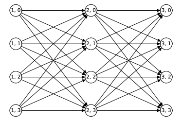
Figure 4: Example for the time-expanded hardware graph $G$ on which the network flow formulation of the TAP is based. The instance is taken from the example in Figure 1. Accordingly, there are $\lvert Q\rvert=4$ logical qubits and $L=3$ time steps. The first number in a node labels the time step while the second number labels the physical qubit.

For our further analysis of the model, we linearize the quadratic Constraints (3.2) by replacing them with

$$y^{t}_{(p,q),(i,j)} \leq w_{p,i}^{t}$$

$$y^{t}_{(p,q),(i,j)} \leq w_{q,j}^{t}$$ (5)

$$y^{t}_{(p,q),(i,j)} \geq w_{p,i}^{t}+w_{q,j}^{t}-1.$$ (6)

From now on, we only consider the linearized version of (3.2)-(3.2) and refer to it as Model (3.2).

Optimal solution to the linear relaxation.

To illustrate the need for the introduction of strengthening inequalities, we show that the linear programming (LP) relaxation of Model (3.2) is very weak in the sense that for any TAP instance there is an optimal LP solution with value $0$. To see this, we assign the flow value $1/\lvert Q\rvert$ to all paths in $G$ with zero costs. More formally, we set

$$x^{t}_{q,i,j} =\begin{cases}1/|Q|,&i=j\\ 0,&i\neq j\end{cases}\qquad\forall i,j\in V,\,\forall q\in Q,\,\forall 1\leq t\leq L-1,$$

$$w^{t}_{q,i} =1/\lvert Q\rvert\quad\forall i\in V,\,\forall q\in Q,\,\forall 1\leq t\leq L$$

and

$$y^{t}_{(p,q),(i,j)} =1/\lvert A_{H}\rvert\quad\forall 1\leq t\leq L,\,\forall(p,q)\in G^{t},\,\forall(i,j)\in A_{H}.$$

It can be checked that this fully symmetrical, fractional solution is valid for the LP relaxation of Model (3.2). Concerning Constraints (3.2), note that $\lvert A_{H}\rvert\geq 2(\lvert Q\rvert-1)\geq\lvert Q\rvert$ and $2/\lvert Q\rvert-1\leq 0$ hold, since $H$ is connected and we have $\lvert Q\rvert\geq 2$.

3.3 Subgraph Isomorphism Inequalities

We will now derive valid inequalities for Model (3.2) to strengthen its LP relaxation. To this end, we extend the result of Lemma 3.7, which we also used in the proof of Theorem 3.8. For a given TAP instance $(H,Q,\Gamma)$, this will enable us to identify a qubit subset $\tilde{Q}\subseteq Q$, an integer distance $d\geq 0$ in $H$ as well as time steps $t_{0}$ and $t_{1}$, between which at least one qubit pair in $\tilde{Q}$ has to move a total distance of at least $d+1$. For the derivation we need

Definition 3.9 ($d$-th relaxed graph).

For an undirected, connected graph $H=(V,E)$ and an integer $d\geq 0$, we define the $d$-th relaxed graph $H^{d}=(V,E^{d})$ as the graph defined by

$$\{i,j\}\in E^{d}\iff d_{H}(i,j)\leq d+1\ .$$

Note that $H^{0}=H$. An example for Definition 3.9 is shown in Figure 5.

(a) $H^{0}=H$

(b) $H^{1}$

(c) $H^{2}$

Figure 5: Example for the $d$-th relaxed graphs $H^{d}$ from Definition 3.9. The graph $H$ is the four-qubit line graph from the example in Figure 1b.

We are now able to sketch the main idea for deriving valid inequalities. Choose a starting time $t_{0}$ and an end time $t_{1}$ with $1\leq t_{0}<t_{1}\leq L$ as well as a subset $\tilde{G}$ of the gates between $t_{0}$ and $t_{1}$. Now, consider the connectivity graph $C(\tilde{G})=(\tilde{Q},E_{C})$. We will relate it to the $d$-th relaxed graph $H^{d}$ of $H$ for some integer $d\geq 0$. Namely, if there is no isomorphism from $C(\tilde{G})$ to some edge-induced subgraph of $H^{d}$, we know that there is no allocation such that all qubits involved in the gates of $\tilde{G}$ are at most an edge distance of $d+1$ apart. Consequently, there has to be at least one gate in $\tilde{G}$ such that the involved qubits are more than $d+1$ apart at $t_{0}$. Between time steps $t_{0}$ and $t_{1}$, this qubit pair will move a total distance of at least $d+1$. This leads us to the following

Lemma 3.10 (Subgraph isomorphism inequalities).

Let $(H,Q,\Gamma)$ be a TAP instance with $H=(V,E)$ and $\Gamma=G^{1},\ldots,G^{L}$. Further, let $\tilde{G}\coloneqq\bigcup_{t=1}^{L}\tilde{G}^{t}$, $\tilde{G}^{t}\subseteq G^{t}$, be a set of gates and let $C\coloneqq C(\tilde{G})=(\tilde{Q},E_{C})$ be the corresponding connectivity graph. Finally, let $d\geq 0$ be an integer and let $H^{d}$ be the $d$-th relaxed graph of $H$. Now consider the time steps $t_{0}\coloneqq\min\{t\mid\tilde{G}^{t}\neq\emptyset\}$ and $t_{1}\coloneqq\max\{t\mid\tilde{G}^{t}\neq\emptyset\}$. If there is no edge-induced subgraph of $H^{d}$ isomorphic to $C$, then the inequalities

$$\sum_{t=t_{0}}^{t_{1}-1}\sum_{q\in\tilde{Q}}\sum_{(i,j)\in V\times V}d_{H}(i,j)x^{t}_{q,i,j} \geq d+1$$ (7)

and

$$\sum_{t=t_{0}}^{t_{1}-1}\sum_{q\in Q}\sum_{(i,j)\in V\times V}d_{H}(i,j)x^{t}_{q,i,j} \geq 2(d+1)$$ (8)

hold.

Proof.

First, we show the validity of (7). For a feasible binary solution to Model (3.2), consider the allocation $a_{t_{0}}$ of qubits at time step $t_{0}$. From $a_{t_{0}}$, construct the edge-induced subgraph $H^{\prime}=(V^{\prime},E^{\prime})$ of $H^{d}=(V,E^{d})$ defined by the edge subset

$$E^{\prime}\coloneqq\left\{\{i,j\}\in E^{d}\mid a_{t_{0}}^{-1}(i),a_{t_{0}}^{-1}(j)\in\tilde{Q}\wedge\{a_{t_{0}}^{-1}(i),a_{t_{0}}^{-1}(j)\}\in E_{C}\right\}.$$ (9)

The mapping defined by the allocation $a_{t_{0}}$ is not an isomorphism from $H^{\prime}$ to $C$, since $C$ is not subgraph isomorphic to $H^{d}$ by assumption. Furthermore, the definition (9) of $E^{\prime}$ implies, that for every edge $\{i,j\}$ in $H^{\prime}$ there is a corresponding edge $\{a_{t_{0}}^{-1}(i),a_{t_{0}}^{-1}(j)\}$ in $C$. This means that there is an edge $\{q_{1},q_{2}\}$ in $C$ such that $\{a_{t_{0}}(q_{1}),a_{t_{0}}(q_{2})\}$ is not an edge in $H^{\prime}$. Thus, $\{a_{t_{0}}(q_{1}),a_{t_{0}}(q_{2})\}$ is also not an edge in $H^{d}$ by equation (9). This edge corresponds to a gate $(q_{1},q_{2})\in G^{t^{\prime}}$ for some $t^{\prime}$ with $t_{0}<t^{\prime}\leq t_{1}$. For this gate, the logical qubits $q_{1}$ and $q_{2}$ are located at physical qubits more than $d+1$ apart at $t_{0}$, i.e.

$$d_{H}(a_{t_{0}}(q_{1}),a_{t_{0}}(q_{2}))>d+1,$$ (10)

but need to be at neighbouring physical qubits at $t^{\prime}$. Thus, together they need to move a distance of at least $d+1$:

$$d_{H}(a_{t_{0}}(q_{1}),a_{t^{\prime}}(q_{1}))+d_{H}(a_{t_{0}}(q_{2}),a_{t^{\prime}}(q_{2})\geq d+1.$$ (11)

This implies (7). Now, we show the validity of (8). For a subset of vertices $\tilde{Q}\subseteq Q$ let

$$L(\tilde{Q})\coloneqq\sum_{q\in\tilde{Q}}d_{H}\left(a_{t_{0}}(q),a_{t^{\prime}}(q)\right)$$ (12)

denote the sum of distances between qubit allocations at $t_{0}$ and qubit allocations at $t^{\prime}$ for logical qubits in $\tilde{Q}$. Then, for the left-hand side of (7) it holds

$$\sum_{t=t_{0}}^{t_{1}-1}\sum_{q\in\tilde{Q}}\sum_{(i,j)\in V\times V}d_{H}(i,j)x^{t}_{q,i,j}\geq L(\tilde{Q}),$$ (13)

since $t^{\prime}\leq t_{1}$. Consider the $Q$-permutation $\pi\coloneqq a_{t_{0}}^{-1}\circ a_{t^{\prime}}\colon Q\rightarrow Q$. Let $K_{1},K_{2}\subseteq Q$ be the cycles in $\pi$ containing $q_{1}$ and $q_{2}$, respectively. First, consider the case $K_{1}\neq K_{2}$. Here it holds

$$L(\tilde{Q})\geq L(K_{1})+L(K_{2})\ ,$$ (14)

since $K_{1}\cap K_{2}=\emptyset$. Furthermore, we know $L(K_{i})\geq 2d_{H}(a_{t_{0}}(q_{i}),a_{t^{\prime}}(q_{i}))$, $i\in\{1,2\}$, since $K_{1}$ and $K_{2}$ are cycles and $d_{H}(\cdot,\cdot)$ satisfies the triangle inequality, see Figure 6a for an illustration.

(a) $K_{1}\neq K_{2}$

(b) $K_{1}=K_{2}$

Figure 6: Sketch for the two cases in the proof of Lemma 3.10. The cycle in (a) contains exactly one of the qubits $q_{1}$ and $q_{2}$ and its length is greater or equal than twice the distance this qubit moves (dashed line). The cycle in (b) contains both qubits $q_{1}$ and $q_{2}$, and its length is greater or equal than twice the initial distance of $q_{1}$ and $q_{2}$ (dashed line).

Thus, we have

$$L(K_{1})+L(K_{2})\geq 2d_{H}(a_{t_{0}}(q_{1}),a_{t^{\prime}}(q_{1}))+2d_{H}(a_{t_{0}}(q_{2}),a_{t^{\prime}}(q_{2}))\overset{\eqref{eq:dist1q2traveled}}{\geq}2(d+1).$$ (15)

On the other hand, if $K_{1}=K_{2}\eqqcolon K$, we find

$$L(\tilde{Q})\geq L(K).$$ (16)

Thus, again using the triangle inequality and the fact that $K$ is a cycle, we have

$$L(K)\geq 2d_{H}(a_{t_{0}}(q_{1}),a_{t_{0}}(q_{2}))\overset{\eqref{eq:distq1q2t0}}{\geq}2(d+1)$$ (17)

as illustrated in Figure 6b. This implies (8). ∎

Clearly, any valid subgraph isomorphism inequality cuts off all solutions of the LP relaxation with zero cost. However, generating these inequalities can be computationally expensive, since subgraph isomorphism is NP-complete.

Having shown its NP-hardness and analysed its binary model, we conclude this section about the TAP by introducing methods to reduce the model size for larger instances.

3.4 Algorithmic Enhancements for Large Instances

To keep the size of Model (3.2) tractable for larger hardware graphs and quantum circuits, we describe two heuristic methods for eliminating variables, which means that both methods may in principle lead to suboptimal solutions. The number of flow variables is decreased by either removing edges from the time-expanded graph $G$ or by removing logical qubits not participating in two-qubit gates.

Limiting Distance.

The first method eliminates edges from $G$. We only consider edges which connect physical qubits in $H$ that are within a given distance limit. Thus, we limit the distance that a logical qubit may move between subsequent allocations. A method to find a reasonable distance limit is to iteratively increase the limit until the TAP becomes feasible. Once the model is feasible, the distance is again increased by one and the TAP is solved a last time.

Limiting the Number of Qubits.

In practice, the number of logical qubits is usually smaller than the number of physical qubits. In principle, this can be reduced to the case of an equal number of logical and physical qubits by adding inactive logical qubits not participating in any two-qubit gates. However, the number of variables in the TAP model grows linearly with $\lvert Q\rvert$. Therefore, we only consider flow variables associated with active logical qubits. This bears the problem that costs associated with the flow of inactive qubits are not counted. To circumvent this issue, we do not allow active logical qubits to change positions with inactive qubits. Thus, the subgraph of $H$ at which active logical qubits are located is fixed for all time steps. However, we stress that the particular choice of this subgraph remains subject to optimization.

4 Solving the Token Swapping Problems

We now turn to the solution of the token swapping problems which need to be solved as the second step in the proposed routing procedure, once an optimal TAP solution has been found. Token swapping is known to be NP-hard (see e.g. [15]). We will develop two solution methods for the token swapping problem: an efficient approximation algorithm as well as an exact branch-and-bound approach.

4.1 Approximate Solution

The proposed qubit routing procedure employs a modified version of the efficient token swapping algorithm given by Miltzow et al. in [15]. This approximation algorithm has running time that is bounded by a polynomial in the number of tokens, also in the worst case. It has a guaranteed approximation factor of four in terms of swap count. However, we note that on all instances we considered, the algorithm exhibits an approximation factor better than 1.5. Indeed, the analysis in [15] shows that the approximation factor is strictly less than four.

We briefly review the original approximation algorithm. For a detailed description and analysis, we refer the interested reader to [15]. Given a token swapping instance $(H,Q,a,a^{\prime})$, the algorithm iteratively performs swaps by gradually changing the allocation from $a$ to $a^{\prime}$. We adapt the notion of [15] for an arbitrary token allocation $\tilde{a}$: an unsatisfied vertex is a vertex $i\in H$ which does not hold its target token, i.e. $\tilde{a}^{-1}(i)\neq(a^{\prime})^{-1}(i)$. A distance-decreasing neighbour of a vertex $i\in H$ is a neighbour of $i$ from which the distance to the target vertex of the token sitting at $i$ is strictly less than the distance from $i$. A happy swap chain of length $k$ is a sequence of $k$ swaps $(i_{1},i_{2}),(i_{2},i_{3}),\ldots,(i_{k-1},i_{k}),(i_{k},i_{k+1})\subseteq\mathcal{T}_{H}$ such that every token involved has its distance decreased after the swaps in the chain have been performed sequentially. An unhappy swap is a swap that moves a token already positioned at its target vertex, while the other token moves closer to its target. Given these notions, the algorithm works as follows:

1. Choose an unsatisfied vertex.

2. Perform a walk along distance-decreasing neighbours until a cycle is closed or a dead end encountered, i.e. no distance-decreasing neighbour exists.

3. Perform the happy swap chain or unhappy swap.

4. Go to 1.

The key insight why this algorithm terminates is, that vertices involved in an unhappy swap will be part of a future happy swap chain. Furthermore, the number of happy swap chains is finite since they necessarily move tokens further towards their targets. The original algorithm, as described in [15], chooses random vertices in steps 1 and 2. We modify the algorithm in two ways aiming to further reduce both resulting swap count and depth. First, in step 1, we choose an unsatisfied vertex that was not part of the previously performed swap chain or unhappy swap. With this choice, we try to reduce depth: only swaps on disjoint vertices can be performed in parallel. Second, we modify step 2. In each step of the walk we try to choose cleverly among all distance-decreasing neighbours by exploring them first. If possible, we choose the one closing the smallest cycle. The motivation for this is, that all swaps in a happy swap chain cannot be performed in parallel since they share common vertices. If no cycle can be closed, we try to avoid dead ends, i.e. unhappy swaps. Intuitively, a typical optimal solution does not use many unhappy swaps.

Having introduced an efficient but approximate method, we now derive an exact branch and bound algorithm.

4.2 Exact Solution

The exact approach will be used for benchmarking the approximation algorithm presented in the previous section. The exact method finds a shortest path from the initial allocation to the final allocation in the associated Cayleigh graph. The latter possesses a node for each of the $\lvert Q\rvert!$ possible allocations. Two nodes are adjacent if and only if there is a swap, i.e. a transposition $\tau\in\mathcal{T}_{H}$, which maps between the associated allocations. It follows that an optimal solution to a token swapping problem is given by a shortest path from the initial allocation to the final allocation in the Cayleigh graph. The search algorithm works through the nodes of the Cayleigh graph starting at the initial allocation. At each node, we give upper and lower bounds on the shortest path length to the goal node. Upper bounding is achieved by running the modified 4-approximation algorithm from Section 4.1, yielding a path from the current node to the goal node. This path is augmented by the path from the start node to the current node, giving a feasible solution to the token swapping problem.

We use two different types of lower bounds, described in the following sections.

4.2.1 Improved Distance Lower Bound

A well-known lower bound on token swapping, already introduced as objective of the TAP in Section 3, is given by

Lemma 4.1 ([28, 15] Distance lower bound).

For any token swapping instance $T=(H,Q,a,a^{\prime})$ it holds

$$\mathrm{OPT}(T)\geq\left\lceil\frac{1}{2}\sum_{q\in Q}d_{H}(a(q),a^{\prime}(q))\right\rceil.$$ (18)

The following Lemma describes a class of instances for which this is bound sharp,i.e. satisfied with equality.

Lemma 4.2.

The distance lower bound (18) is sharp on all token swapping instances that require two or less swaps.

Proof.

It is easy to see that the bound is sharp for an instance that requires one or less swaps. Now, consider an instance that requires two swaps. Here, exactly a two cases can occur. Either the two swaps act on disjoint vertices, or they share a common vertex. In the first case, the sum in (18) amounts to 4, where in the second case it amounts to at least 3. ∎

A simple example for a token swapping instance requiring two swaps is given by a 3-vertex line graph where initially no vertex holds its desired token. On the contrary, for every optimal objective value greater or equal to 3, one can construct token swapping instances, for which the distance bound is not sharp. On a complete (sub-)graph, place $n$ tokens such that the underlying permutation has exactly one cycle. Then, an optimal solution has $n-1$ swaps as we will see in the following section. However, the distance bound is $\left\lceil n/2\right\rceil<n-1$ for $\geq 3$.

Lemma 4.2 implies that the decomposition of the qubit routing problem into TAP and token swapping is guaranteed to return optimal solutions for all instances that have a solution with two or less swaps. Our aim is now to improve upon lower bound (18). To this end, we introduce the notion of a blocking vertex.

Definition 4.3 (Blocking vertex).

Let $(H,Q,a,a^{\prime})$ be a token swapping instance. Let $q\in Q$ be a token not yet sitting at its target vertex, i.e. $a(q)\neq a^{\prime}(q)$. A vertex $v\in H$ is called $q$-blocking vertex if it is contained in a shortest path in $H$ from $a(q)$ to $a^{\prime}(q)$, and if it holds its desired token i.e. $a^{-1}(v)=(a^{\prime})^{-1}(v)$.

Intuitively, the presence of blocking vertices increases the number of required swaps. This intuition is confirmed by

Lemma 4.4 (Improved distance lower bound).

Let $T=(H,Q,a,a^{\prime})$ be a token swapping instance. Let $Q^{*}\subseteq Q$ denote the set of tokens not yet sitting at their target vertices. For every $q\in Q^{*}$ let $B_{q}\subset V$ be a set of $q$-blocking vertices (see Definition 4.3) of size $k_{q}$ such that

1. any path in $H$ from $q$ to its target vertex avoiding any of the blocking vertices in $B_{q}$ has at least length $d_{H}(a(q),a^{\prime}(q))+2k_{q}$ and

2. the sets $B_{q}$ are pairwise disjoint.

Then it holds

$$\mathrm{OPT}({\color[rgb]{0,0,1}T})\geq\left\lceil\sum_{q\in Q}\frac{d_{H}(a(q),a^{\prime}(q))}{2}\right\rceil+\sum_{q\in Q^{*}}k_{q}.$$ (19)

Figure 7: Sketch for the proof of Lemma 4.4. The shortest path from the vertex holding token $q$ to its target vertex (horizontal arrow) is blocked by vertices already holding their desired tokens (black circles). In any solution, $q$ takes a detour (curved arrow) or satisfied tokens at blocking vertices are moved. Either alternative results in additional swaps.

Proof.

Consider a solution $\mathcal{S}=\tau_{1},\tau_{2},\ldots,\tau_{N}$ and denote $[N]\coloneqq\{1,\ldots,N\}$. We partition $Q^{*}=Q^{*}_{1}\,\dot{\cup}\,Q^{*}_{2}$ according to the following scheme: for $q\in Q^{*}$ let $q\in Q^{*}_{1}$ if the path of $q$ in $\mathcal{S}$ contains all associated blocking vertices $B_{q}$; otherwise, let $q\in Q^{*}_{2}$.

For $q\in Q_{2}^{*}$ and $v,v^{\prime}\in V$ let $\mathcal{P}_{q}(v,v^{\prime})$ denote the set of $v$-$v^{\prime}$-paths in $H$ which do not contain all of the blocking vertices $B_{q}$. For a path $p\in\mathcal{P}_{q}(v,v^{\prime})$, define its length as $l(p)\coloneqq\lvert p\rvert-1$. Moreover, define

$$d_{H,q}(v,v^{\prime})\coloneqq\min\{l(p)\mid\in\mathcal{P}_{q}(v,v^{\prime})\}$$ (20)

as the minimum edge-distance between $v$ and $v^{\prime}$ if only paths not containing all $q$-blocking vertices are allowed. Note, that $\mathcal{P}_{q}(a(q),a^{\prime}(q))\neq\emptyset$: from the definition of $Q^{*}_{2}$, it follows that for all $q\in Q^{*}_{2}$ there is a path not containing $B_{q}$. Furthermore, by property (i) of $B_{q}$ it holds

$$d_{H,q}(a(q),a^{\prime}(q))\geq d_{H}(a(q),a^{\prime}(q))+2k_{q},$$ (21)

for all $q\in Q^{*}_{2}$, see Figure 7 for an illustration.

For $i\in[N]$, consider the sum $d_{i}$ of all edge distances from tokens in $Q^{*}$ to their targets after swap $\tau_{i}$ has been performed, accounting for the detours taken by tokens in $Q^{*}_{2}$,

$$d_{i}\coloneqq \sum_{q\in Q^{*}_{1}}d_{H}(\tau_{i}\circ\tau_{i-1}\circ\ldots\circ\tau_{1}\circ a(q),a^{\prime}(q))+$$

$$\sum_{q\in Q^{*}_{2}}d_{H,q}(\tau_{i}\circ\tau_{i-1}\circ\dots\circ\tau_{1}\circ a(q),a^{\prime}(q)).$$

Accordingly, set

$$d_{0}\coloneqq\sum_{q\in Q_{1}^{*}}d_{H}(a(q),a^{\prime}(q))+\sum_{q\in Q^{*}_{2}}d_{H,q}(a(q),a^{\prime}(q)).$$ (22)

Using (21) yields

$$d_{0}\geq\sum_{q\in Q^{*}}d_{H}(a(q),a^{\prime}(q))+\sum_{q\in Q^{*}_{2}}2k_{q}=\underbrace{\sum_{q\in Q}d_{H}(a(q),a^{\prime}(q))}_{\eqqcolon D_{0}}+\sum_{q\in Q^{*}_{2}}2k_{q},$$ (23)

where we used that $d_{H}(a(q),a^{\prime}(q))=0$ for all $q\in Q\setminus Q^{*}$. Furthermore, for $i\in[N]$ let $\Delta d_{i}$ denote the difference

$$\Delta d_{i}\coloneqq d_{i}-d_{i-1}.$$ (24)

Clearly, $d_{N}=0$, since $\tau_{N}\circ\ldots\circ\tau_{2}\circ\tau_{1}\circ a=a^{\prime}$. Thus,

$$\sum_{i\in[N]}\Delta d_{i}=d_{N}-d_{0}=-d_{0}.$$ (25)

Furthermore, for any $i\in[N]$ it holds $-2\leq\Delta d_{i}\leq 2$, since a swap moves two tokens each for a distance of 1.

Now, we turn to $Q_{1}^{*}$. By definition of $Q_{1}^{*}$, a vertex $v\in\bigcup_{q\in Q^{*}_{1}}B_{q}$ is necessarily involved in a swap. For $v\in\bigcup_{q\in Q^{*}_{1}}B_{q}$, denote by $i_{v}\coloneqq\min\{i\in[N]\mid v\in\tau_{i}\}$ the first swap that involves $i$. Let $I\coloneqq\{i_{v}\mid v\in\bigcup_{q\in Q^{*}_{1}}B_{q}\}$. Partition $I=I_{0}\,\dot{\cup}\,I_{2}$ in the following way. For $i_{v}\in I$, if there is an $v^{\prime}\in\bigcup_{q\in Q^{*}_{1}}B_{q}$ such that $v^{\prime}\neq v$ but $i_{v}=i_{v^{\prime}}$, we let $i_{v}$ belong to the set $I_{2}$. Otherwise, we let $i_{v}$ belong to the set $I_{0}$. Then, for $i\in I_{0}$ we have $\Delta d_{i}\geq 0$, since at least one token leaves its target vertex by swap $\tau_{i}$, namely the token $a^{-1}(v)$. Furthermore, for $i\in I_{2}$ we have $\Delta d_{i}=2$, since both tokens leave their target vertices by swap $\tau_{i}$.

Let $n_{0}\coloneqq\lvert I_{0}\rvert$ and $n_{2}\coloneqq\lvert I_{2}\rvert$. Using property (ii) of $B_{q}$ and the definition of $I_{0}$ and $I_{2}$, it holds

$$\lvert\bigcup_{q\in Q^{*}_{1}}B_{q}\rvert=\sum_{q\in Q^{*}_{1}}k_{q}=2n_{2}+n_{0}.$$ (26)

Let $\bar{I}\coloneqq[N]\setminus{I}=[N]\setminus(I_{0}\cup I_{2})$. Then we can use (25) to obtain

$$-d_{0}=\sum_{i\in[N]}\Delta d_{i} =\underbrace{\sum_{i\in I_{0}}\Delta d_{i}}_{\geq 0}+\underbrace{\sum_{i\in I_{2}}\Delta d_{i}}_{=2n_{2}}+\sum_{i\in\bar{I}}\Delta d_{i}\geq 2n_{2}+\sum_{i\in\bar{I}}\Delta d_{i}.$$ (27)

Thus, with (23), we have

$$\sum_{i\in\bar{I}}\Delta d_{i}\leq-D_{0}-\sum_{q\in Q^{*}_{2}}2k_{q}-2n_{2}.$$ (28)

Since $\Delta d_{i}\geq-2$, it follows

$$\lvert\bar{I}\rvert\geq\left\lceil\frac{D_{0}+\sum_{q\in Q^{*}_{2}}2k_{q}+2n_{2}}{2}\right\rceil=\left\lceil\frac{D_{0}}{2}\right\rceil+\sum_{q\in Q^{*}_{2}}k_{q}+n_{2}.$$ (29)

Altogether, this means

$$N =\lvert I_{0}\rvert+\lvert I_{2}\rvert+\lvert\bar{I}\rvert\geq n_{0}+n_{2}+\left\lceil\frac{D_{0}}{2}\right\rceil+\sum_{q\in Q^{*}_{2}}k_{q}+n_{2}$$

$$=\left\lceil\frac{D_{0}}{2}\right\rceil+\sum_{q\in Q^{*}_{2}}k_{q}+\sum_{q\in Q^{*}_{1}}k_{q}=\left\lceil\frac{D_{0}}{2}\right\rceil+\sum_{q\in Q^{*}}k_{q}\ .$$

∎

The question remains, how the sets of blocking vertices $B_{q}$ can be computed in practise. We employ a simple greedy procedure that iterates over all tokens and takes as many blocking vertices as possible in each iteration. As it turns out computationally, this lower bound is particularly strong on graphs with low connectivity. On the contrary, the second lower bound employed by the branch-and-bound algorithm is stronger on dense graphs.

4.2.2 Complete Split Graph Lower Bound

While the bound from Lemma 4.4 is based on relaxing the restriction, that tokens need to be moved by swaps, we now derive a lower bound that is based on relaxing the set of allowed transpositions $\mathcal{T}_{H}$. This set is increased by adding edges missing in $H$. We use a result of Yasui et al. ([29]), who give an efficient algorithm for solving token swapping problems on complete split graphs.

Definition 4.5 (Complete split graph).

A vertex subset of a graph is called independent if no two vertices in the subset are connected by an edge. A vertex subset is called a clique if any two vertices in the subset are connected by an edge. A graph is called a complete split graph if it can be partitioned into an independent set and a clique such that every vertex in the independent set is connected to all vertices in the clique.

Lemma 4.6 (Complete split graph lower bound [29]).

Let $T=(H,Q,a,a^{\prime})$ be a token swapping instance. Furthermore, let $V^{\prime}\subset V$ be an independent set in $H$. Let $n=\lvert V\rvert$ be the number of vertices, let $r$ be the number of cycles in the permutation $a\circ(a^{\prime})^{-1}$ including fix points, i.e. cycles of length 1. Let $q$ be the number of cycles in the permutation $a\circ(a^{\prime})^{-1}$ excluding fix points that only involve vertices in $V^{\prime}$. Then it holds

$$\mathrm{OPT}(T)\geq n-r+2q.$$ (30)

Proof.

Consider the graph $H^{\prime}=(V,E^{\prime})$ which is derived from $H$ and $V^{\prime}$ in the following way: connect every vertex in $V^{\prime}$ with all vertices in $V\setminus V^{\prime}$. Additionally, add all missing edges in $V\setminus V^{\prime}$. Then $H^{\prime}$ is a complete split graph. Furthermore, $E\subseteq E^{\prime}$ holds, and thus also $\mathcal{T}_{H}\subseteq\mathcal{T}_{H}^{\prime}$. Consider a solution $\mathcal{S}$ of size $N$ to $T$. This is also a solution to the token swapping instance $T^{\prime}\coloneqq(H^{\prime},Q,a\circ(a^{\prime})^{-1},\mathrm{id})$. Thus, we have

$$\lvert\mathcal{S}\rvert\geq\mathrm{OPT}(T^{\prime}).$$ (31)

According to [29], the optimal value for $T^{\prime}$ is given by

$$\mathrm{OPT}(T^{\prime})=n-r+2q.$$ (32)

Thus,

$$\lvert\mathcal{S}\rvert\geq n-r+2q.$$ (33)

∎

We remark that Lemma 4.6 is a generalization of the well-known fact that token swapping on complete graphs has optimal value $n-r$ (cf. e.g. [12]). When applying Lemma 4.6 in practise, an independent set needs to be constructed first. In our implementation, we employ a simple greedy procedure that iterates over the vertices increasing in degree, adding it to the independent set if possible.

As already mentioned, both lower bounds complement each other: while the distance bound is strong on sparse graphs, the complete-split-graph bound is strong on dense graphs. The following lemma allows to increase the lower bounds from Lemmas 4.4 and 4.6 by one in some cases.

Lemma 4.7 (Parity of solutions).

Let $T=(H,Q,a,a^{\prime})$ be a token swapping instance. Let $\mathrm{sgn}(\pi)$ denote the sign of a permutation $\pi$. For any solution $\mathcal{S}=\tau_{1},\tau_{2},\ldots,\tau_{N}$ to $T$, it holds

$$N\equiv\left[1-\mathrm{sgn}(a^{\prime}\circ a^{-1})\right]/2\mod 2$$ (34)

Proof.

For any solution $\mathcal{S}$, it holds

$$a^{\prime}=\tau_{N}\circ\ldots\circ\tau_{2}\circ\tau_{1}\circ a$$ (35)

or, equivalently

$$a^{\prime}\circ a^{-1}=\tau_{N}\circ\ldots\circ\tau_{2}\circ\tau_{1}.$$ (36)

Using the fact that $\mathrm{sgn}(\sigma\circ\pi)=\mathrm{sgn}(\sigma)\cdot\mathrm{sgn}(\pi)$ for any two permutations $\sigma,\pi$, we have

$$\mathrm{sgn}(a^{\prime}\circ a^{-1})=\mathrm{sgn}(\tau_{N})\cdots\mathrm{sgn}(\tau_{2})\cdot\mathrm{sgn}(\tau_{1})=(-1)^{N}.$$

Thus, $N$ is either even or odd, independent of $S$:

$$N\equiv\left[1-\mathrm{sgn}(a^{\prime}\circ a^{-1})\right]/2\mod 2.$$ (37)

∎

With these theoretical properties of our solution method to the qubit routing by swap insertion problem established, we now present various experimental results.

5 Experimental Results

In the following, we benchmark the proposed routing algorithm. We perform experiments covering four aspects:

1. The computation time and solution quality when solving the TAP model with strengthening inequalities.

2. The quality and speed of the token swapping approximation algorithm.

3. The quality of the routing solution produced by the combined algorithm compared to other routing methods.

4. The quality of solutions produced by quantum algorithms compiled with our routing method, executed on actual quantum hardware.

The datasets generated and analyzed during the current study are available from the corresponding author on reasonable request.

5.1 Benchmarking the Strengthened TAP Model

In the first step of the proposed decomposition approach, a TAP needs to be solved. Here, we give numerical results showing how the introduction of subgraph isomorphism cutting planes (Section 3.3) can accelerate the solution of the TAP binary linear program. The linearized flow model (3.2) is implemented and solved via the Python API of Gurobi ([8]). Before parsing the model to the solver, we generate a set of valid inequalities introduced in Section 3.3. These are added to a cut pool. The solver can add cuts from this pool to the model in order to cut off relaxed solutions.

The set of valid inequalities is generated as follows: first, the graphs $H^{d}$ for $0\leq d\leq\max_{i,j\in H}d_{H}(i,j)$ are created and transformed into their respective line graphs. To generate a subset of gates for which a valid cut may be derived, we first choose time steps $t_{0}$ and $t_{1}$ such that $1\leq t_{0}<t_{1}\leq L$. Then, all gates in gate groups between $t_{0}$ and $t_{1}$ are considered. The corresponding connectivity graph is generated and transformed into its line graph. To perform the node-induced-subgraph isomorphism check, we employ an implementation of the VF2 algorithm (see [4, 3]) from the NetworkX python package ([9]). This procedure is repeated by iterating over time steps $t_{0}$, $t_{1}$ until all possible time step pairs have been checked.

In the first benchmark, we measure the computation time required for solving TAP instances to optimality. We compare the total time taken with strengthening inequalities to the time taken for the bare model (3.2). We measure the ratio $r_{t}=t_{\mathrm{SGI}}/t_{\mathrm{bare}}$, where $t_{\mathrm{SGI}}$ and $t_{\mathrm{bare}}$ are the runtimes of the strengthened model and the bare model, respectively. The time consumed by cutting plane generation lies between $0.1$ s and 20 s and is included in the total runtime $t_{\mathrm{SGI}}$.

In all instances $(H,Q,\Gamma)$, the hardware graph $H$ has 8 vertices and $Q\coloneqq\{q_{1}\ldots,q_{8}\}$. Tests are performed on four hardware graphs with different sparsity, namely the line, ring, Y and ladder graph, illustrated in Fig 8. Each of the gate groups in $\Gamma=G^{1},G^{2},\ldots,G^{L}$ consists of $\left\lfloor L/2\right\rfloor$ randomly chosen pairs of qubits among the set $\{q_{1},\cdots,q_{L}\}$. This results in instances with as many gates per time step as possible, making the instances computationally hard. The depth $L$ is varied from 4 to 8, where 10 instances are generated per value of $L$. The instance sizes resemble the capabilities of currently available quantum hardware. All instances are solved to optimality. The absolute solutions times lie between 0.6 s and 1000 s. Results are given in Table 1a. Shorter average runtimes are achieved for $L=5$ on ring, Y, and ladder. A maximum saving of to 72% is observed for the $L=4$ line. Furthermore, we observe rather high differences between minimum and maximum runtime ratio, indicating a strong instance dependence. Summarizing, the separation of valid subgraph isomorphism inequalities can improve the TAP-model runtime. Thus, also the algorithm for the full routing problem benefits from generating valid inequalities for the TAP subproblem. However, the strong instance dependence suggests that more research is necessary in order to fully exploit the potential of subgraph isomorphism inequalities.

For the same benchmark set, we measure the tightness of the lower bound on the number of required swaps in an optimal routing solution, given by the optimal TAP solution. To this end, the objective of the full routing model (BIP) from [18] is adjusted to minimize swap count instead of depth. Solving this model yields the optimal swap number. We measure the relative bound $r_{b}=\frac{\mathrm{OPT}_{\mathrm{TAP}}}{\mathrm{OPT}_{\mathrm{BIP}}}$, with $\mathrm{OPT}_{\mathrm{BIP}}$ and $\mathrm{OPT}_{\mathrm{TAP}}$ denoting the optimal BIP solution and TAP solution, respectively. These results are shown in Table 1b. We observe tight bounds with a relative difference of at most 23% ($L=8$ line), together with small deviations from the average value. This is a key feature of our decomposition approach: optimal TAP solution values typically give a good estimate for the number of required swaps.

(a) Line

(b) Ring

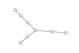
(c) Y

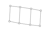
(d) Ladder

Figure 8: Hardware graphs used in the benchmarks of Sec. 5.1 and Sec. 5.3.

	$L$
	4			5			6			7			8
$H$	min	max	avg	min	max	avg	min	max	avg	min	max	avg	min	max	avg
Line	0.28	3.9	1.31	0.8	2.56	1.28	1.27	7.76	2.96	0.31	4.19	2.49	0.47	2.35	1.35
Ring	0.5	0.98	1.02	0.64	1.9	0.8	0.76	3.72	1.56	0.74	2.78	1.34	0.48	1.47	1.01
Y	0.48	1.58	1.16	0.49	2.76	0.87	0.75	2.54	1.49	0.77	3.39	1.89	0.56	2.87	1.74
Ladder	0.36	1.16	1.2	0.48	2.47	0.9	0.78	9.72	2.62	0.63	4.58	2.4	0.93	7.26	2.53

(a) Rutnime comparison when solving to optimality.

	$L$
	4			5			6			7			8
$H$	min	max	avg	min	max	avg	min	max	avg	min	max	avg	min	max	avg
Line	1.0	1.0	1.0	0.8	1.0	0.98	0.9	1.0	0.98	0.85	1.0	0.95	0.77	1.0	0.86
Ring	1.0	1.0	1.0	0.8	1.0	0.98	1.0	1.0	1.0	1.0	1.0	1.0	0.92	1.0	0.97
Y	1.0	1.0	1.0	0.8	1.0	0.94	0.89	1.0	0.96	0.85	1.0	0.93	0.81	1.0	0.89
Ladder	1.0	1.0	1.0	1.0	1.0	1.0	1.0	1.0	1.0	0.8	1.0	0.94	0.83	1.0	0.97

(b) Bound quality when solving to optimality.

Table 1: TAP-model benchmark results. The different hardware graphs, denoted $H$, are depicted in Fig. 8. The qubit set is $Q\coloneqq\{q_{1}\ldots,q_{8}\}$. Each instance contains $L$ many gate groups $G^{1},G^{2},\ldots,G^{L}$, where each gate group consists of $\left\lfloor L/2\right\rfloor$ randomly chosen pairs of qubits among the set $\{q_{1},\cdots,q_{L}\}$. 10 instances are generated per depth $L$ and graph $H$. Each instance is solved with and without additional strengthening inequalities. We compare the ratio $r_{t}$ of runtimes in (a). Additionally, in (b) we give the relative bound quality $r_{b}$ for the optimal TAP value as a lower bound on the number of required swaps in an optimal routing solution.

5.2 Benchmarking the Token Swapping Approximation

The second step in the decomposition approach consists of several consecutive token swapping instances. Here, we evaluate the performance of the employed token swapping approximation. All algorithms described in this section have been implemented in Python from scratch. First, we compare the original 4-approximation algorithm given in [15] to our modified version. For this purpose, we generate random token swapping instances, i.e. initial and final allocations on three types of planar graphs with different sparsity. As graph types we choose ring graphs, ladders and square meshes with node numbers of 16, 36 and 64 for each type. As in the previous section, this choice of graph types and sizes aims at resembling current realizations of quantum computer hardware connectivity graphs. We generate 100 instances per graph. In Table 2, we give the average ratio $r_{\#}$ of swap numbers between the modified version and the original version as well as the average ratio of depths $r_{d}$ .

	Ring		Ladder		Mesh
$N$	$r_{\#}$	$r_{d}$	$r_{\#}$	$r_{d}$	$r_{\#}$	$r_{d}$
16	0.96	0.91	0.88	0.82	0.81	0.78
36	1.0	1.0	0.91	0.83	0.83	0.78
64	1.0	0.99	0.93	0.79	0.84	0.81

Table 2: Comparison of original and modified token swapping approximation algorithms. We give the average ratio of inserted swaps $r_{\#}=\#_{\text{mod}}/\#_{\text{orig}}$ and resulting depths $r_{d}=d_{\text{mod}}/d_{\text{orig}}$. Comparison are made on rings, ladders and meshes with increasing vertex number $N$.

Firstly, note that these ratios are less than or equal to $1$ across all instances. This means that our modification always performs as least as good as the original version, or better (if the factor is smaller than $1$). Furthermore, both swap and depth ratio are roughly constant across graph sizes for a given graph type. However, the advantage of the modified version increases with growing connectivity of the graph type. An intuitive explanation of this behaviour is the increase of swapping possibilities with growing edge number. This allows the modified version to employ its potential of deciding for “good” swaps instead of choosing them randomly.

Secondly, we compare the modified 4-approximation algorithm to the exact branch-and-bound algorithm in terms of runtime and solution quality. We measure the approximation ratio $r_{\#}=\#_{\text{approx}}/\#_{\text{opt}}$ as well as the runtime ratio $r_{t}=t_{\text{approx}}/t_{\text{bnb}}$ on various instances. As graph types, we choose lines, rings and ladders. Again, this choice tries to resemble real hardware graphs while we also want to make use of the fact that token swapping can be solved efficiently on lines and rings. This allows use to measure the approximation quality for instances which are intractable for the exact algorithm. Experimental results are summarized in Table 3.

First, we observe that for lines the approximation ratio is unity across all instances. As it might be conjectured from these numerical results, one can also convince oneself theoretically that the approximation algorithm always finds an optimal solution on lines.

Furthermore, Table 3 shows that for ring and ladder graphs the average approximation ratio is less than or equal to 1.25, which is well below the theoretical value of 4. This indicates that the theoretical approximation factor of 4 underestimates the approximation quality observed in practice. As already mentioned, the proof in [15] delivers an approximation ratio of strictly less than four.

Comparing runtimes, we note a drastic improvement with growing graph size on all graph types. For the largest instances the exact algorithm was able to solve in reasonable time, an average reduction of 96.5% is achieved. Moreover, all absolute runtimes for the approximation algorithm are well below 1 s. Altogether, the approximation algorithm typically delivers close-to-optimal solutions with a significant time saving on all instances considered.

	Line			Ring			Ladder
$N$	$r_{\#}$	$r_{t}$	$\bar{t}_{\text{appr}}$	$r_{\#}$	$r_{t}$	$\bar{t}_{\text{appr}}$	$r_{\#}$	$r_{t}$	$\bar{t}_{\text{appr}}$
5	1.0	0.2	0.0	1.25	0.3	0.0	1.04	0.6	0.0
10	1.0	0.05	0.0	1.19	0.2	0.0	1.19	0.2	0.0
12	1.0	-	0.0	1.23	0.08	0.0	1.13	0.035	0.0
50	1.0	-	0.8	1.17	-	0.4			0.4

Table 3: Comparison of token swapping approximation and exact algorithm. We give the average approximation ratio $r_{\#}=\#_{\text{appr}}/\#_{\text{opt}}$ and runtime ratio $r_{t}=t_{\text{appr}}/t_{\text{bnb}}$ as well as the average absolute runtime of the approximation algorithm $\bar{t}_{\text{appr}}$ in seconds. Instance graphs are lines, rings and ladders of increasing vertex number $N$. Token swapping can be solved efficiently on lines and rings, cf. [12]. This allows us to compare approximation ratios even when the runtime is intractable for the exact algorithm (indicated by “-”). For ladders, no efficient exact algorithm exists. Therefore, no results are presented for large ladder graphs (empty cells). Averages are taken over 100 random instances. Exceptions due to excessive runtime are: 54 instances for $N=10$ lines, 22 for $N=12$ rings and 18 for $N=12$ ladders.

5.3 Benchmarking the Routing Algorithm

In the following, the proposed routing method (abbreviated TAP+TS) is compared to various routing algorithms integrated in different open source quantum compilers: The binary program (BIP) by Nannicini et al. ([18]), solved via Gurobi, Li et al.’s Sabre heuristic ([14]), Qiskit’s default compiler Stochastic swap ([20]), Cambridge Quantum Computing’s Tket ([5, 23]), Google’s Cirq [2], as well as the Bounded mapping tree (BMT) by Siraichi et. al ([21]) which is based on a decomposition approach similar to ours. BMT employs dynamic programming to solve a problem closely related to the TAP.

We briefly summarize the Python implementation of our routing algorithm: first, the two-qubit gates of the input circuit are grouped in layers containing as much gates as possible. These gate groups together with the hardware graph form a TAP instance. Next, the network flow model of the TAP instance is solved by Gurobi. The resulting TAP solution defines a set of token swapping problems, which are then solved by the approximation algorithm described in Section 4. Finally, the routed quantum circuit is constructed by changing the target qubits in the gates of the original circuit according to the allocation sequence and by adding the computed swaps between subsequent allocations.

As performance metrics, we measure the resulting gate count and circuit depth. Benchmarks are performed on two different classes of circuits. The first class is taken from a publicly available benchmark library while the second is generated according to a protocol used for benchmarking quantum hardware.

QUEKO circuits.

First, we use the publicly available benchmarks circuits generated by Tan and Cong in [24]. They propose a method for generating random circuits on a given hardware graph with given depth as well as given single and two-qubit gate numbers. Their construction delivers instances of the routing by swap insertion problem with optimal value $0$, i.e. there exists an allocation of logical to physical qubits such that all gates can be performed without inserting swaps.

We use the “benchmark for near-term feasibility” (BNTF) circuit set from [24]. It is subdivided into circuits on a 16-qubit hardware graph (Rigetti’s Apsen-4, Fig. 9a) with few gates, and circuits on a 54 qubit graph (Google’s Sycamore, Fig. 9b) with many gates. For each hardware graph, 90 circuits are available – 10 for each depth in $\{5,10,\ldots,45\}$. On each instance the time limit for BIP is the set to 3600 s. The results are visualized in Figure 10. By construction, our algorithm will find a zero-swap solution if the TAP is solved to optimality. This can be observed in Figures 10a and 10b. For this benchmark set, we achieve improvements in resulting depth of up to a factor of 2 on small circuits (Figure 10c) and up to factor of 5 on larger circuits (Figure 10d), compared to the best heuristic. This improvement comes at the cost of increased runtime. Indeed, the runtimes of all other heuristics applied in this benchmark are in the order of a few seconds (not shown in Figure 10), while the proposed algorithm takes up to 12 s on average for small circuits (Figure 10e) and up to 5 min on average for larger circuits (Figure 10f). However, we note a drastic reduction of runtime compared to the exact approach BIP (Figure 10e) which is unable to find optimal solutions on larger instances in less than one hour.

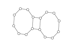
(a)

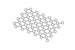
(b)

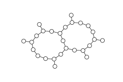
(c)

Figure 9: Hardware graphs of Aspen-4 (a), Sycamore (b) and ibmq_ehningen (c).

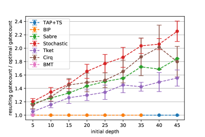
(a) Gatecount comparison on Aspen-4.

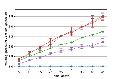
(b) Gatecount comparison on Sycamore.

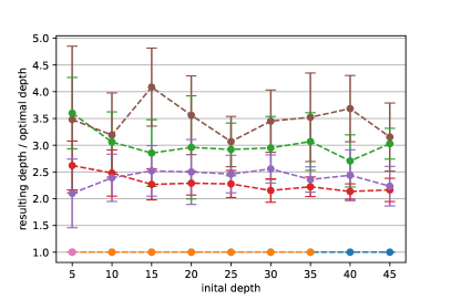
(c) Depth comparison on Aspen-4.

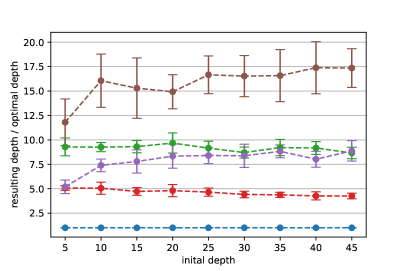
(d) Depth comparison on Sycamore.

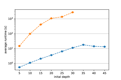
(e) Runtime comparison on Aspen-4.

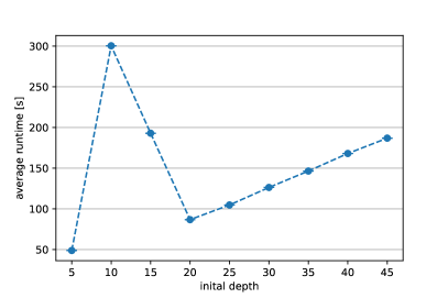
(f) Runtime comparison on Sycamore.

Figure 10: Comparison of different routing algorithms on the QUEKO benchmark set. Data points are averaged over 10 instances. Error bars indicate the empirical standard deviation. The legend in (a) holds for all plots. Instances are the BNTF circuits from [24] on Rigetti’s Aspen-4 16-qubit hardware graph (left plots) as well as Google’s Sycamore 54-qubit hardware graph (right plots). For every BNTF instance, a zero-swap solution exists. Missing data points for BIP and BMT indicate that no solution was returned after 3600 s runtime. (a), (b): Gatecount relative to optimum. (c), (d): Depth relative to optimum. (e), (f): Average runtime for BIP and BMT. Other heuristics are not shown since all runtimes are in the order of 1 s.

QV circuits.

For a second benchmark, we consider quantum volume (QV) circuits. According to [16], a QV circuit of depth $L$ and width $m$ is a circuit on $m$ qubits with $L$ layers where each layer consists of $\lfloor m/2\rfloor$ random two-qubit gates. Thus, the resulting circuit is maximally dense in terms of gates per layer. QV circuits of equal depth and width are used to benchmark quantum computers (see [6]). We consider QV circuits of equal depth and width. Circuits are constructed from the gate groups of the TAP instances generated in Sec 5.1 resulting in QV circuits with depths between $L=4$ and $L=8$. As in Sec. 5.1, tests are performed on a 8-vertex-line, ring, Y and ladder graph. Thus, the TAP instances associated with the routing instances generated here are exactly those of Sec. 5.1.

Optimal-depth solutions cannot be calculated in reasonable time for all instances. However, BIP would find optimal solutions in terms of depth when solved to optimality. Thus, we measure resulting depth and gate count relative to the BIP solution with a runtime limit of 7200 s. Our results are visualized in Figures 11 and 12. In Figures 11c, 11d, 12c and 12d we observe that the proposed algorithm finds solutions which are close-to-optimal in terms of depth, assuming BIP returned an optimal-depth solution after a runtime of 7200 s. The average ratio of TAP+TS solution to BIP solution is at most 1.25%. Furthermore, it performs best among all considered routing heuristics, in particular better than the conceptually similar method BMT. This also holds true when comparing gate numbers, as can be seen in Figures 11a, 11b, 12a and 12b. Interestingly, we observe that the proposed method delivers smaller gate numbers than BIP for some instances on all topologies, as indicated by values less than 1 in Figures 11a, 11b, 12a and 12b. Again, the improvement comes at the cost of increased runtime. While the other heuristics require several seconds (not shown in Figs. 11,12), the proposed method takes up to 900 s on average (Figure 11f). Still, the runtime is significantly shorter than for the exact method BIP which runs into the time limit of 7200 s on large instances (Figures 11f, 12f).

We discuss three reasons why the improved routing solutions can be worth the additional time investment. First, access to currently available quantum hardware is often organized by a waiting queue, such that the time for compilation is not a critical factor. Second, different quantum circuits with equal connectivity graphs only need to be routed once. A popular example are parameterized quantum circuits which are often considered as promising candidates for first quantum applications. The connectivity graph of such a circuit is not parameter dependent. Third, current quantum hardware benefits strongly from good routing solutions. This is demonstrated in the next section.

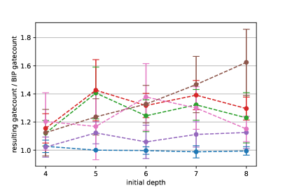
(a) Gatecount comparison on line.

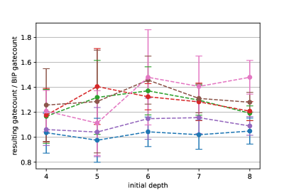
(b) Gatecount comparison on ring.

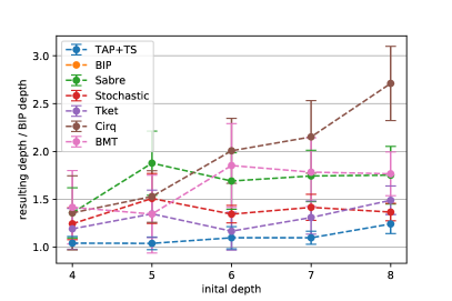
(c) Depth comparison on line.

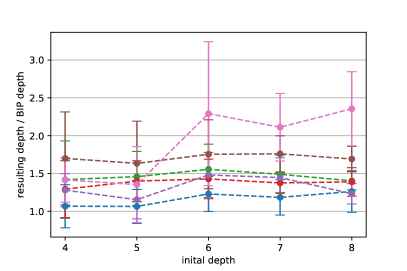
(d) Depth comparison on ring.

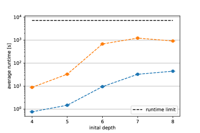
(e) Runtime comparison on line.

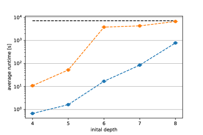
(f) Runtime comparison on ring.

Figure 11: Comparison of different routing algorithms on the QV benchmark set. Instances are QV circuits of equal width and depth ([6, 16]) on a 8-vertex line (left plots) and a 8-vertex ring (right plots). Data points are averaged over 10 instances. Error bars indicate the empirical standard deviation. The legend in (c) holds for all plots. (a), (b): Gate count relative to BIP. (c), (d): Depth relative to BIP. (e), (f): Average runtime. The dashed line indicates the runtime limit of 7200 s. Other heuristics are not shown since their runtimes are in the order of 1 s.

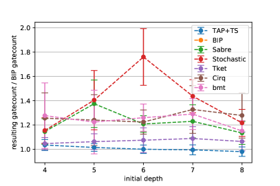
(a) Gatecount comparison on Y graph.

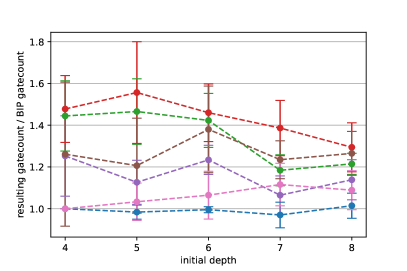
(b) Gatecount comparison on ladder.

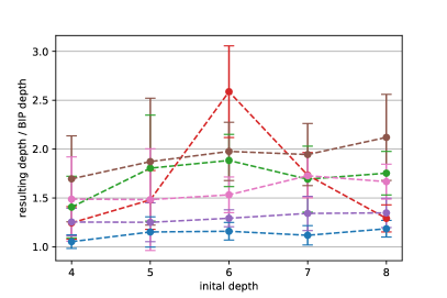
(c) Depth comparison on Y graph.

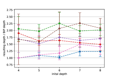
(d) Depth comparison on ladder.

(e) Runtime comparison on Y graph.

(f) Runtime comparison on ladder.

Figure 12: Comparison of different routing algorithms on the QV benchmark set. Instances are QV circuits of equal width and depth ([6, 16]) on a 8-vertex Y-graph (left plots) and a 8-vertex ladder-graph (right plots). Data points are averaged over 10 instances. Error bars indicate the empirical standard deviation. The legend in (a) holds for all plots. (a), (b): Gate count relative to BIP. (c), (d): Depth relative to BIP. (e), (f): Average runtime. The dashed line indicates the runtime limit of 7200 s. Other heuristics are not shown since their runtimes are in the order of 1 s.

5.4 Performance on Real Hardware

Lastly, we demonstrate the influence of routing quality on the performance of current quantum hardware. For this purpose, we compile example quantum algorithms to a real hardware device using different routing methods and compare the results after execution.

The example algorithms are the Quantum approximate optimization algorithm (QAOA) with depth parameter $p=1$ applied to MaxCut on ring graphs with 7, 8 and 9 vertices. QAOA is a well-known hybrid quantum-classical algorithm. A detailed description is given by Farhi et al. in [7]. We choose QAOA for three reasons: First, it is often considered as a promising candidate for near-term quantum applications because of its universality and adaptive complexity. Second, routing is an essential requirement when running QAOA on real hardware, since QAOA employs two-qubit gates along the edges of an underlying problem graph which usually is not isomorphic to the hardware connectivity graph. This is also the case in our experiment. Third, the approximation ratio of QAOA is an easily accessible, single-metric performance measure. The approximation ratio is defined as $r=\mathbbm{E}(c)/c^{*}$. Here $\mathbbm{E}(c)$ denotes the expectation value of the cut size $c$ produced by QAOA, and $c^{*}$ is the size of an optimal cut. QAOA is a parameterized quantum algorithm. For QAOA with depth $p=1$ applied to MaxCut on ring graphs, the optimal parameters can be calculated analytically, cf. [25].

The routing algorithms tested are the proposed method TAP+TS, Tket and Stochastic swap. For circuit construction, compilation and backend communication, we use IBM’s SDK Qiskit ([20]). The quantum backend in our experiment is ibmq_ehnigen ([10]), see Fig. 9c. We compile each of the QAOA circuits with all three routing methods while other compiler options remain unchanged.

Table 4 compares the gate counts and depths of the compiled circuits as well as the achieved approximation ratios after execution on ibmq_ehnigen. The proposed routing procedure TAP+TS performs best both in terms of swaps added and depth increase on all instances, followed by Tket. For the instance with $N=8$, we note large reductions in gate count of 65% and 69% when compared to Tket and Stochastic swap, respectively. Similarly, the circuit depth reductions amount to 60% and 68%, respectively. We observe that small gate count and depth correlate with an increase of approximation ratio on all instances. For the $N=8$ instance, we observe an increase of 23% compared to TKet. The influence of depth and gate count on noise in quantum computers are currently investigated in depth by different groups. Although the relations are not yet fully understood, this experiment shows a clear correlation between routing quality and quantum algorithm performance.

Of course, this experiment is by no means a comprehensive benchmark of our routing method. However, it stresses the need for good compiling methods in quantum computation on currently available hardware and shows clear benefits of our approach.

$N$	$\#_{2q}^{\text{TAP+TS}}$	$\#_{2q}^{\text{Tket}}$	$\#_{2q}^{\text{Sto}}$	$d^{\text{TAP+TS}}$	$d^{\text{Tket}}$	$d^{\text{Sto}}$	$r_{\text{ideal}}$	$r_{\text{TAP+TS}}$	$r_{\text{Tket}}$	$r_{\text{St}}$
7	21	31	54	22	28	41	0.875	0.77	0.61	0.56
8	25	71	80	21	53	65	0.75	0.64	0.52	0.51
9	30	54	63	21	39	45	0.84	0.65	0.58	0.55

Table 4: Results for compiling quantum algorithms to real hardware with different routing algorithms. Compiled quantum circuits are QAOA for MaxCut on ring graphs with $N$ vertices. The target quantum device is ibmq_ehningen. Given are the total two-qubit gate counts $\#_{2q}^{\text{TAP+TS}}$, $\#^{\text{Tket}}_{2q}$, $\#_{2q}^{\text{Sto}}$ for the circuit routed with TAP+TS, Tket and Stochastic swap, respectively, as well as the corresponding depths $d^{\text{TAP+TS}}$, $d^{\text{Tket}}$, $d^{\text{Sto}}$. Furthermore, we give the theoretical approximation ratio $r_{\text{ideal}}$ as well as the actually achieved approximation ratios $r_{\text{TAP+TS}}$, $r_{\text{Tket}}$, $r_{\text{St}}$.

6 Conclusion

In this article, we have studied the problem of qubit routing by swap insertion. This problem needs to be solved in the context of quantum compilation but is practically intractable even for moderate instance sizes when solved by an exact approach. We have proposed a new decomposition approach that exploits the capabilities of exact integer programming while reducing complexity significantly, at the expense of possibly returning suboptimal solutions. Improvement in performance is achieved by solving only a subproblem by integer programming. The objective of this subproblem, called token allocation problem (TAP), is a lower bound on the overall routing problem. We strengthened the model of the TAP by deriving valid inequalities. The solution of the TAP defines the second subproblem, which is the well-known problem of token swapping. Its solution yields the actual objective value of the overall routing problem. For the token swapping problem, we have enhanced an existing approximation algorithm and have developed an exact branch-and-bound algorithm. Combining the solutions of both subproblems produces a solution to the overall routing problem.

Finally, we have given experimental results showing the applicability of the proposed algorithm. Although it being a heuristic approach, we observed close-to-optimal solutions outperforming other heuristics. This improvement comes at the expense of increased solution time; however, the solution time is still much smaller than for exact approaches. Moreover, the lower bounds computed in the TAP turn out to be tight, which we consider as a reason for the good performance of the proposed decomposition method.

Our experiments on actual quantum hardware show the impact of high-quality solutions to qubit routing for quantum computation on current hardware. For the example algorithm QAOA, we observed an increase in approximation ratio when compiled with the proposed routing method compared to standard heuristics.

A possible field of future research is the structural analysis of the TAP in order to further strengthen its integer programming formulation. Additionally, practical experience with current quantum hardware suggests more complicated cost functions to be considered: specific qubits and gates suffer from higher error rates than others. Even more complicated, executing gates on specific qubit pairs simultaneously results in high error rates – a phenomenon known as crosstalk. Incorporating these effects in the routing algorithm is an additional direction of future research.

References

- [1] A. M. Childs, E. Schoute, and C. M. Unsal. Circuit Transformations for Quantum Architectures. In W. van Dam and L. Mancinska, editors, 14th Conference on the Theory of Quantum Computation, Communication and Cryptography (TQC 2019), volume 135 of Leibniz International Proceedings in Informatics (LIPIcs), pages 3:1–3:24, Dagstuhl, Germany, 2019. Schloss Dagstuhl–Leibniz-Zentrum für Informatik. URL: http://drops.dagstuhl.de/opus/volltexte/2019/10395, doi:10.4230/LIPIcs.TQC.2019.3.
- [2] Cirq. https://quantumai.google/cirq, Aug. 2021. doi:10.5281/zenodo.5182845.
- [3] L. P. Cordella, P. Foggia, C. Sansone, and M. Vento. An improved algorithm for matching large graphs. In 3rd IAPR-TC15 Workshop on Graph-based Representations in Pattern Recognition, Cuen, pages 149–159, 2001.
- [4] L. P. Cordella, P. Foggia, C. Sansone, and M. Vento. A (sub)graph isomorphism algorithm for matching large graphs. IEEE Transactions on Pattern Analysis and Machine Intelligence, 26(10):1367–1372, 2004. doi:10.1109/TPAMI.2004.75.
- [5] A. Cowtan, S. Dilkes, R. Duncan, A. Krajenbrink, W. Simmons, and S. Sivarajah. On the Qubit Routing Problem. In W. van Dam and L. Mancinska, editors, 14th Conference on the Theory of Quantum Computation, Communication and Cryptography (TQC 2019), volume 135 of Leibniz International Proceedings in Informatics (LIPIcs), pages 5:1–5:32, Dagstuhl, Germany, 2019. Schloss Dagstuhl–Leibniz-Zentrum für Informatik. URL: http://drops.dagstuhl.de/opus/volltexte/2019/10397, doi:10.4230/LIPIcs.TQC.2019.5.
- [6] A. W. Cross, L. S. Bishop, S. Sheldon, P. D. Nation, and J. M. Gambetta. Validating quantum computers using randomized model circuits. Physical Revue A, 100:032328, 2019. URL: https://link.aps.org/doi/10.1103/PhysRevA.100.032328, doi:10.1103/PhysRevA.100.032328.
- [7] E. Farhi, J. Goldstone, and S. Gutmann. A quantum approximate optimization algorithm, 2014. arXiv:1411.4028.
- [8] Gurobi Optimization, LLC. Gurobi Optimizer Reference Manual, 2022. URL: https://www.gurobi.com.
- [9] A. A. Hagberg, D. A. Schult, and P. J. Swart. Exploring network structure, dynamics, and function using networkx. In G. Varoquaux, T. Vaught, and J. Millman, editors, Proceedings of the 7th Python in Science Conference, pages 11 – 15, Pasadena, CA USA, 2008. URL: http://conference.scipy.org/proceedings/SciPy2008/paper_2/.
- [10] IBM Quantum. https://quantum-computing.ibm.com/, 2021.
- [11] S. Johnstun and J.-F. Van Huele. Understanding and compensating for noise on IBM quantum computers. American Journal of Physics, 89(10):935–942, 2021. arXiv:https://doi.org/10.1119/10.0006204, doi:10.1119/10.0006204.
- [12] D. Kim. Sorting on graphs by adjacent swaps using permutation groups. Computer Science Review, 22:89–105, 2016. URL: https://www.sciencedirect.com/science/article/pii/S1574013716300077, doi:https://doi.org/10.1016/j.cosrev.2016.09.003.
- [13] A. Kissinger and A. M.-V. D. Griend. CNOT circuit extraction for topologically-constrained quantum memories. Quantum Information and Computation, 20(7/8):581–596, 2020.
- [14] G. Li, Y. Ding, and Y. Xie. Tackling the qubit mapping problem for NISQ-era quantum devices. In Proceedings of the Twenty-Fourth International Conference on Architectural Support for Programming Languages and Operating Systems, ASPLOS ’19, page 1001–1014, New York, NY, USA, 2019. Association for Computing Machinery. doi:10.1145/3297858.3304023.
- [15] T. Miltzow, L. Narins, Y. Okamoto, G. Rote, A. Thomas, and T. Uno. Approximation and Hardness of Token Swapping. In P. Sankowski and C. Zaroliagis, editors, 24th Annual European Symposium on Algorithms (ESA 2016), volume 57 of Leibniz International Proceedings in Informatics (LIPIcs), pages 66:1–66:15, Dagstuhl, Germany, 2016. Schloss Dagstuhl–Leibniz-Zentrum für Informatik. URL: http://drops.dagstuhl.de/opus/volltexte/2016/6408, doi:10.4230/LIPIcs.ESA.2016.66.
- [16] N. Moll, P. Barkoutsos, L. S. Bishop, J. M. Chow, A. Cross, D. J. Egger, S. Filipp, A. Fuhrer, J. M. Gambetta, M. Ganzhorn, A. Kandala, A. Mezzacapo, P. Müller, W. Riess, G. Salis, J. Smolin, I. Tavernelli, and K. Temme. Quantum optimization using variational algorithms on near-term quantum devices. Quantum Science and Technology, 3(3):030503, 2018. doi:10.1088/2058-9565/aab822.
- [17] L. Moro, M. G. A. Paris, M. Restelli, and E. Prati. Quantum compiling by deep reinforcement learning. Communications Physics, 4(1):178, Aug 2021. doi:10.1038/s42005-021-00684-3.
- [18] G. Nannicini, L. S. Bishop, O. Günlük, and P. Jurcevic. Optimal qubit assignment and routing via integer programming, 2021. arXiv:2106.06446.
- [19] M. A. Nielsen and I. L. Chuang. Quantum Computation and Quantum Information: 10th Anniversary Edition. Cambridge University Press, 2010. doi:10.1017/CBO9780511976667.
- [20] Qiskit. An open-source framework for quantum computing. http://www.qiskit.org, 2021. doi:10.5281/zenodo.2573505.
- [21] M. Y. Siraichi, V. F. d. Santos, C. Collange, and F. M. Q. a. Pereira. Qubit allocation as a combination of subgraph isomorphism and token swapping. Proc. ACM Program. Lang., 3(OOPSLA), Oct 2019. doi:10.1145/3360546.
- [22] M. Y. Siraichi, V. F. d. Santos, C. Collange, and F. M. Quintão Pereira. Qubit Allocation. In CGO 2018 - International Symposium on Code Generation and Optimization, pages 1–12, Vienna, Austria, Feb 2018. URL: https://hal.archives-ouvertes.fr/hal-01655951, doi:10.1145/3168822.
- [23] S. Sivarajah, S. Dilkes, A. Cowtan, W. Simmons, A. Edgington, and R. Duncan. tket: a retargetable compiler for NISQ devices. Quantum Science and Technology, 6(1):014003, 2020. doi:10.1088/2058-9565/ab8e92.
- [24] B. Tan and J. Cong. Optimality study of existing quantum computing layout synthesis tools. IEEE Transactions on Computers, 70(9):1363–1373, 2021. doi:10.1109/TC.2020.3009140.
- [25] Z. Wang, S. Hadfield, Z. Jiang, and E. Rieffel. The quantum approximation optimization algorithm for MaxCut: A fermionic view. Physical Review A, 97:022304, 2017. doi:10.1103/PhysRevA.97.022304.
- [26] I. Wegener. Complexity Theory: Exploring the Limits of Efficient Algorithms, page 81. Springer Berlin Heidelberg, 2005. doi:https://doi.org/10.1007/3-540-27477-4.
- [27] R. Wille, L. Burgholzer, and A. Zulehner. Mapping quantum circuits to IBM QX architectures using the minimal number of SWAP and H operations. In Design Automation Conference, 2019.
- [28] K. Yamanaka, E. D. Demaine, T. Ito, J. Kawahara, M. Kiyomi, Y. Okamoto, T. Saitoh, A. Suzuki, K. Uchizawa, and T. Uno. Swapping labeled tokens on graphs. Theoretical Computer Science, 586:81–94, 2015. URL: https://www.sciencedirect.com/science/article/pii/S0304397515001656, doi:https://doi.org/10.1016/j.tcs.2015.01.052.
- [29] G. Yasui, K. Abe, K. Yamanaka, and T. Hirayama. Swapping labeled tokens on complete split graphs. IPSJ SIG Technical Report, 14, 2015.
- [30] A. Zulehner, A. Paler, and R. Wille. An efficient methodology for mapping quantum circuits to the ibm qx architectures. IEEE Transactions on Computer-Aided Design of Integrated Circuits and Systems, 38(7):1226–1236, 2019. doi:10.1109/TCAD.2018.2846658.