Spatial frequency of unstable eigenfunction of the core-periphery model with transport cost of differentiated agriculture

Abstract

The core-periphery model with transport cost of differentiated agriculture is extended to continuously multi-regional space, and the stability of a homogeneous stationary solution of the model on a periodic space is investigated. When a spatial disturbance around the homogeneous stationary solution is decomposed into eigenfunctions, an unstable area, defined as the area of parameters where each eigenfunction is unstable, is observed to generally expand in its size as the frequency number of each eigenfunction increases.

Keywords:  continuous racetrack economy; economic agglomeration; differentiated agricultural goods; new economic geography; self-organization; transport cost

JEL classification: Q10, R12, R40, C62, C63, C68

1 Introduction

The core-periphery (CP) model proposed by Krugman (1991) provides a sophisticated language based on general equilibrium theory for various fields involved in more or less market-economic and geographic phenomena, such as urban economics, regional economics, international economics, and regional science. The model has allowed these disciplines to be studied in a unified approach and has actually brought about the development of them in various directions, such as the formation of urban systems, population and industrial agglomeration, and international trade.

In the most basic formulation of the model, agricultural goods are assumed to be undifferentiated, and, in addition, their transport is assumed to have no cost. Then, symmetric equilibrium, where all regions are uniformly populated, is stable when the transport cost is sufficiently high, while it becomes unstable when the transport cost is sufficiently low, producing a spatially inhomogeneous structure. Meanwhile, Fujita et al. (1999, Chapter 7) introduce a model incorporating differentiated agriculture and its transport cost. This model has an interesting property that symmetric equilibrium stabilizes not only when the manufacturing transport cost is sufficiently high but also when the manufacturing transport cost is sufficiently low.

We extend the CP model with differentiated agriculture and its transport cost to infinitely multi-regional space, and investigate the stability of a stationary solution in the case of periodic one-dimensional case. In the continuous space model, small disturbances to the stationary solution are decomposed into the Fourier series, and each eigenfunction that composes the series has an integer number of its own spatial frequency. The value of the spatial frequency corresponds to the number of cities or economic centers formed when workers and capitals begin to agglomerate.

Depending on the value of various parameters, there would be eigenfunctions that are stable over the entire range of manufacturing transport cost (stable eigenfunctions). On the other hand, there are eigenfunctions that become unstable at certain manufacturing transport cost values (unstable eigenfunctions). We see that unstable eigenfunctions can be stable when manufacturing transport cost is sufficiently high, but become unstable when the cost is lower than a certain threshold value of the transport cost (upper critical point). As the transport cost decreases further below another threshold (lower critical point), the eigenfunction becomes stable again. The behavior of these unstable eigenfunctions is similar to the solution of a linear problem around a homogeneous stationary solution of the original two-regional model by Fujita et al. (1999, Chapter 7).

Furthermore, we obtain expression for the eigenvalue corresponding to the eigenfunction of each frequency and investigate its frequency-dependent behavior. From numerical observations, it is suggested that as the spatial frequency number of the eigenfunction increases within the even-only or odd-only range, the upper critical point would be non-decreasing (generally increasing) and the lower critical point would be non-increasing (generally decreasing), resulting in expansion of the unstable area where the eigenvalue takes positive value. Meanwhile, it is often observed that the value of lower critical point become larger with increasing frequency that are not limited to even or odd numbers. Nevertheless, if the frequency increases sufficiently, the unstable area generally expands.

There are several important related literature. Ottaviano and Thisse (2004, Section 5) and Picard and Zeng (2005) consider a quasi-linear model that takes into account differentiated agriculture and its transport cost. In addition, Zeng and Takatsuka (2016) and Zeng (2021) even treat the case of a footloose entrepreneur model. In international trade theory, models including agriculture and its cost have also been devised. For example, Takatsuka and Zeng (2012) consider the transport cost of the homogeneous agricultural sector, and Zeng and Kikuchi (2009) deal with the transport cost of differentiated agriculture. Most relevant to the current paper is the study by Gallego and Zofío (2018) that analyzes an impact of international trade on domestic agglomeration based on the multi-regional CP model that considers the differentiated agriculture with its transport cost. Their model is an extension of the discrete space version of the model treated in the current paper to international trade. The current paper, however, deals with the continuous-space model in which possible agglomeration locations are not fixed in advance, and focuses on examining in detail the frequencies of the eigenfunctions that govern the behavior of the economic agglomeration when the homogeneous state becomes unstable and economic agglomeration emerges.

The rest of the paper is organized as follows. Section 2 derives the model. Section 3 discusses the homogeneous stationary solution and the eigenvalue of the linearized problem around the stationary solution. Section 4 examines how the eigenvalues depend on various parameters, mainly frequency. Section 5 discuses the results and gives conclusions. Section 6 gives modeling and proofs of several propositions omitted in the main part.

2 The model

The model which we handle is the following nonlinear system of integral-differential equations given by

$$\left\{\begin{aligned} &Y(t,x)=\mu w^{M}(t,x)\lambda(t,x)+(1-\mu)w^{A}(t,x)\phi(x),\\ &G^{A}(t,x)=\left[\int_{\mathcal{S}}\phi(y){w^{A}(t,y)}^{1-\eta}{T^{A}(x,y)}^{1-\eta}dy\right]^{\frac{1}{1-\eta}},\\ &w^{A}(t,x)=\left[\int_{\mathcal{S}}Y(t,y){G^{A}(t,y)}^{\eta-1}{T^{A}(x,y)}^{1-\eta}dy\right]^{\frac{1}{\eta}},\\ &G^{M}(t,x)=\left[\int_{\mathcal{S}}\lambda(t,y){w^{M}(t,y)}^{1-\sigma}{T^{M}(x,y)}^{1-\sigma}dy\right]^{\frac{1}{1-\sigma}},\\ &w^{M}(t,x)=\left[\int_{\mathcal{S}}Y(t,y){G^{M}(t,y)}^{\sigma-1}{T^{M}(x,y)}^{1-\sigma}dy\right]^{\frac{1}{\sigma}},\\ &\omega(t,x)=w^{M}(t,x){G^{M}(t,x)}^{-\mu}{G^{A}(t,x)}^{\mu-1},\\ &\frac{\partial}{\partial t}\lambda(t,x)=\gamma\left[\omega(t,x)-\int_{\mathcal{S}}\omega(t,y)\lambda(t,y)\right]\lambda(t,x)\end{aligned}\right.$$ (1)

with an initial condition $\lambda(0,x)=\lambda_{0}(x)\geq 0,~{}(\forall x\in\mathcal{S})$ which satisfies $\int_{\mathcal{S}}\lambda_{0}(x)dx=1$.

Here, $\mathcal{S}$ is a $d$ ($\geq 1$)-dimensional continuous manifold. The parameters $\mu\in(0,1)$, $\eta>1$ and $\sigma>1$ stand for the degree to which the consumer values the manufacturing goods, the elasticity of substitution between any two varieties of agricultural goods and that of manufactured goods, respectively. The speed at which population moves between regions is proportional to $\gamma>0$. The mobile workers are continuously distributed on $\mathcal{S}$ and the density at time $t\in[0,\infty)$, region $x\in{\mathcal{S}}$ is denoted by $\mu\lambda(t,x)\geq 0$ which satisfies $\int_{\mathcal{S}}\lambda(t,x)dx\equiv 1$ for any time $t\in[0,\infty)$. The immobile workers are also distributed on $\mathcal{S}$ and the density at region $x\in{\mathcal{S}}$ is denoted by $(1-\mu)\phi(x)\geq 0$ which satisfies $\int_{\mathcal{S}}\phi(x)dx\equiv 1$. The nominal wages of the immobile and mobile workers at time $t$ at region $x$ are denoted by $w^{A}(t,x)$ and $w^{M}(t,x)$, respectively. Thus, the density of income $Y(t,x)$ at $t$ at $x$, is represented by the first equation in (1). The functions $T^{A}(x,y)\geq 1$ and $T^{M}(x,y)\geq 1$ represent the amount of agricultural and manufacturing goods that must be shipped to transport one unit of the agricultural and manufacturing goods, respectively, from $x$ to $y$. The real wage at $t$ at $x$ is denoted by $\omega(t,x)$.

In the following, we consider in particular a circumference $S$ of radius $r>0$ as a manifold $\mathcal{S}$ and discuss the system (1) on $S$. The iceberg-functions are also restricted to the forms

$$T^{A}(x,y)=e^{\tau_{A}|x-y|},$$ (2)

$$T^{M}(x,y)=e^{\tau_{M}|x-y|},$$

respectively, where $\tau_{A}\geq 0$ and $\tau_{M}\geq 0$ are cost parameters. Here, the distance function $|x-y|$ is defined as the shorter distance between $x$ and $y$ along the circumference $S$. Then, the parameters $\tau_{A}$ , $\tau_{M}$, $\eta$, and $\sigma$ often appear in the form $\tau_{A}(\eta-1)$ and $\tau_{M}(\sigma-1)$, so it is convenient to define

$$\alpha=\tau_{A}(\eta-1)\geq 0,$$

$$\beta=\tau_{M}(\sigma-1)\geq 0.$$

In the following, we identify a function on $S$ with a corresponding periodic function on the interval $[-\pi,\pi]$, that is, $Y(t,x)$, $G^{A}(t,x)$, $w^{A}(t,x)$, $G^{M}(t,x)$, $w^{M}(t,x)$, $\omega(t,x)$, and $\lambda(t,x)$ of $(t,x)\in[0,\infty)\times S$ are identified with the corresponding functions which are periodic with respect to spatial variables $Y(t,\theta)$, $G^{A}(t,\theta)$, $w^{A}(t,\theta)$, $G^{M}(t,\theta)$, $w^{M}(t,\theta)$, $\omega(t,\theta)$, and $\lambda(t,\theta)$ of $(t,\theta)\in[0,\infty)\times[-\pi,\pi]$, respectively. In fact, this identification is possible in the following way. In general, an element $x\in S$ corresponds one-to-one to an element $\theta\in[-\pi,\pi]$, i.e.,

$$x=x(\theta),$$

so for any function $f$ on $S$, there exists a corresponding periodic function $\tilde{f}$ on $[-\pi,\pi]$ such that

$$f(x)=f(x(\theta))=\tilde{f}(\theta).$$

Then, integral of $f$ on $S$ is calculated by

$$\int_{S}f(x)dx=\int_{-\pi}^{\pi}\tilde{f}(\theta)rd\theta.$$

The distance between $x=x(\theta)$ and $y=y(\theta^{\prime})$ is calculated by

$$|x-y|=r\times\min\left\{|\theta-\theta^{\prime}|_{\rm abs},2\pi-|\theta-\theta^{\prime}|_{\rm abs}\right\},$$

where $|\cdot|_{\rm abs}$ stands for the absolute value.

3 Stationary solution

This section considers a homogeneous stationary solution and a linearized system of (1) on $S$ with (2) around the stationary solution.

3.1 Homogeneous stationary solution

We find the homogeneous stationary solution such that all variables $Y$, $w^{A}$, $G^{A}$, $w^{M}$, $G^{M}$, and $\omega$ are spatially uniform. Then, $\lambda$ and $\phi$ should be

$$\lambda(t,x)\equiv\overline{\lambda}=\frac{1}{2\pi r},$$

$$\phi(x)\equiv\overline{\phi}=\frac{1}{2\pi r}.$$

From the first equation of (1), stationary $Y$ becomes

$$\overline{Y}=\mu\overline{w}^{M}\overline{\lambda}+(1-\mu)\overline{w}^{A}\overline{\phi}.$$ (3)

From the second equation of (1), stationary $G^{A}$

$$\overline{G}^{A} =\left[\overline{\phi}{\overline{w}^{A}}^{1-\eta}E_{\alpha}\right]^{\frac{1}{1-\eta}}.$$ (4)

Here, $E_{\alpha}$ is defined by

$$E_{\alpha}=\int_{S}e^{-\alpha|x-y|}dy=\frac{2(1-e^{-\alpha r\pi})}{\alpha}.$$

From the third equation of (1), stationary $w^{A}$ becomes

$$\overline{w}^{A} =\left[\overline{Y}{\overline{G}^{A}}^{\eta-1}E_{\alpha}\right]^{\frac{1}{\eta}}$$ (5)

Then, (5) together with (3) and (4) yield

$${\overline{w}^{A}}={\overline{w}^{M}}(=:\overline{w}).$$

This gives, from (3),

$$\overline{Y}=\frac{\overline{w}}{2\pi r}.$$

From the fourth equation of (1), stationary $G^{M}$ becomes

$${\overline{G}^{M}} =\left[\overline{\lambda}\overline{w}^{1-\sigma}E_{\beta}\right]^{\frac{1}{1-\sigma}}$$ (6)

Here $E_{\beta}$ is defined by

$$E_{\beta}=\int_{S}e^{-\beta|x-y|}dy=\frac{2(1-e^{-\beta r\pi})}{\beta}.$$

From the sixth equation of (1) together with (4), (5) and (6), stationary $\omega$ is given by

$$\overline{\omega} =\overline{\lambda}^{\frac{\mu}{\sigma-1}}\overline{\phi}^{\frac{1-\mu}{\eta-1}}E_{\alpha}^{\frac{1-\mu}{\eta-1}}E_{\beta}^{\frac{\mu}{\sigma-1}}.$$

3.2 Linearization

Let $\Delta Y(t,x)$, $\Delta G^{A}(t,x)$, $\Delta w^{A}(t,x)$, $\Delta G^{M}(t,x)$, $\Delta w^{M}(t,x)$, $\Delta\omega(t,x)$, and $\Delta\lambda(t,x)$ for $t\in[0,\infty)$ and $x\in S$ be small perturbations. Substituting $Y(t,x)=\overline{Y}+\Delta Y(t,x)$, $G^{A}(t,x)=\overline{G}^{A}+\Delta G^{A}(t,x)$, $w^{A}(t,x)=\overline{w}+\Delta w^{A}(t,x)$, $G^{M}(t,x)=\overline{G}^{M}+\Delta G^{M}(t,x)$, $w^{M}(t,x)=\overline{w}+\Delta w^{M}(t,x)$, $\omega(t,x)=\overline{\omega}+\Delta\omega(t,x)$, and $\lambda(t,x)=\overline{\lambda}+\Delta\lambda(t,x)$ into (1), and ignoring higher order terms, we obtain the following linearized system

$$\left\{\begin{aligned} &\Delta Y(t,x)=\mu\overline{w}\Delta\lambda+\mu\overline{\lambda}\Delta w^{M}(t,x)+(1-\mu)\overline{\phi}\Delta w^{A}(t,x),\\ &\Delta G^{A}(t,x)=\frac{\overline{w}^{-\eta}{\overline{G}^{A}}^{\eta}}{2\pi r}\int_{S}\Delta w^{A}(t,y)e^{-\alpha|x-y|}dy,\\ &\Delta w^{A}(t,x)=\frac{\eta-1}{\eta}\overline{Y}\overline{w}^{1-\eta}{\overline{G}^{A}}^{\eta-2}\int_{S}\Delta G^{A}(t,y)e^{-\alpha|x-y|}dy\\ &\hskip 88.20354pt+\frac{{\overline{G}^{A}}^{\eta-1}\overline{w}^{1-\eta}}{\eta}\int_{S}\Delta Y(t,y)e^{-\alpha|x-y|}dy,\\ &\Delta G^{M}(t,x)={\overline{G}^{M}}^{\sigma}\overline{\lambda}\overline{w}^{-\sigma}\int_{S}\Delta w^{M}(t,y)e^{-\beta|x-y|}dy\\ &\hskip 96.73936pt+\frac{{\overline{G}^{M}}^{\sigma}}{1-\sigma}\overline{w}^{1-\sigma}\int_{S}\Delta\lambda(t,y)e^{-\beta|x-y|}dy,\\ &\Delta w^{M}(t,x)=\frac{\sigma-1}{\sigma}\overline{w}^{1-\sigma}\overline{Y}{\overline{G}^{M}}^{\sigma-2}\int_{S}\Delta G^{M}(t,y)e^{-\beta|x-y|}dy\\ &\hskip 93.89409pt+\frac{\overline{w}^{1-\sigma}}{\sigma}{\overline{G}^{M}}^{\sigma-1}\int_{S}\Delta Y(t,y)e^{-\beta|x-y|}dy,\\ &\Delta\omega(t,x)=-\mu\overline{\omega}{\overline{G}^{M}}^{-1}\Delta G^{M}(t,x)-(1-\mu)\overline{\omega}{\overline{G}^{A}}^{-1}\Delta G^{A}(t,x)\\ &\hskip 196.324pt+\overline{\omega}\overline{w}^{-1}\Delta w^{M}(t,x),\\ &\frac{\partial}{\partial t}\Delta\lambda(t,x)=\gamma\overline{\lambda}\Delta\omega(t,x).\end{aligned}\right.$$ (7)

The Fourier expansion of a periodic function $\tilde{f}$ on $[-\pi,\pi]$, which is identified with the corresponding function $f$ on $S$, is given by

$$\tilde{f}(\theta)=\frac{1}{2\pi}\sum_{n=0}^{\infty}\hat{f}_{n}e^{in\theta}$$

where $\hat{f}_{n},~{}n=0,\pm 1,\pm 2,\cdots$ are the Fourier coefficients defined by

$$\hat{f}_{n}=\int_{-\pi}^{\pi}\tilde{f}(\theta^{\prime})e^{-in\theta^{\prime}}d\theta^{\prime}.$$

Let $\hat{Y}_{n}$, $\hat{G}^{A}_{n}$, $\hat{w}^{A}_{n}$, $\hat{G}^{M}_{n}$, $\hat{w}^{M}_{n}$, $\hat{\omega}_{n}$, and $\hat{\lambda}_{n}$ be the Fourier coefficients for $\Delta Y(t,\theta)$, $\Delta G^{A}(t,\theta)$, $\Delta w^{A}(t,\theta)$, $\Delta G^{M}(t,\theta)$, $\Delta w^{M}(t,\theta)$, $\Delta\omega(t,\theta)$, and $\Delta\lambda(t,\theta)$, respectively. By (7), we obtain the following equation of the Fourier coefficients

$$\left\{\begin{aligned} &\hat{Y}_{n}=\mu\overline{w}\hat{\lambda}_{n}+\mu\overline{\lambda}\hat{w}^{M}_{n}+(1-\mu)\overline{\phi}\hat{w}^{A}_{n},\\ &\hat{G}^{A}_{n}=\overline{w}^{-1}\overline{G}^{A}H^{\alpha}_{n}\hat{w}^{A}_{n},\\ &\hat{w}^{A}_{n}=\frac{\eta-1}{\eta}\overline{w}{\overline{G}^{A}}^{-1}H^{\alpha}_{n}\hat{G}^{A}_{n}+\frac{2\pi r}{\eta}H^{\alpha}_{n}\hat{Y}_{n},\\ &\hat{G}^{M}_{n}=\frac{\overline{G}^{M}}{\overline{w}}H^{\beta}_{n}\hat{w}^{M}_{n}+\frac{2\pi r}{1-\sigma}\overline{G}^{M}H^{\beta}_{n}\hat{\lambda}_{n},\\ &\hat{w}_{n}^{M}=\frac{\sigma-1}{\sigma}\frac{\overline{w}}{\overline{G}^{M}}H^{\beta}_{n}\hat{G}^{M}_{n}+\frac{2\pi r}{\sigma}H^{\beta}_{n}\hat{Y}_{n},\\ &\hat{\omega}_{n}=-\mu\overline{\omega}{\overline{G}^{M}}^{-1}\hat{G}^{M}_{n}-(1-\mu)\overline{\omega}{\overline{G}^{A}}^{-1}\hat{G}^{A}_{n}+\overline{\omega}\overline{w}^{-1}\hat{w}^{M}_{n},\\ &\frac{\partial}{\partial t}\hat{\lambda}_{n}=\gamma\overline{\lambda}\hat{\omega}_{n}\end{aligned}\right.$$ (8)

for $n=\pm 1,\pm 2,\cdots$. Solving the first six equations of (8), we get

$$\hat{\omega}_{n}=\Omega_{n}\hat{\lambda}_{n}.$$

Here,

$$\Omega_{n} =\frac{2\pi r\overline{\omega}}{(\sigma-1)D}\left[\left\{-\frac{\sigma(\mu^{2}+b)}{b}+1+B\right\}{H^{\beta}_{n}}^{2}\right.$$ (9)

$$\hskip 76.82243pt\left.+\frac{\mu(\sigma(b+1)-1)}{b}H^{\beta}_{n}-B\right],$$

where

$$b=1-\frac{(1-\mu)H^{\alpha}_{n}}{\eta-(\eta-1){H^{\alpha}_{n}}^{2}},$$ (10)

$$B=\frac{\mu\sigma(\sigma-1)(1-b)H^{\alpha}_{n}}{b},$$ (11)

$$D=\sigma-\frac{\mu}{b}H^{\beta}_{n}-(\sigma-1){H^{\beta}_{n}}^{2}$$ (12)

with $H^{\alpha}_{n}$ and $H^{\beta}_{n}$ defined by

$$H^{\alpha}_{n}=\frac{\alpha^{2}r^{2}\left(1-(-1)^{|n|}e^{-\alpha r\pi}\right)}{(n^{2}+\alpha^{2}r^{2})(1-e^{-\alpha r\pi})}$$

and

$$H^{\beta}_{n}=\frac{\beta^{2}r^{2}\left(1-(-1)^{|n|}e^{-\beta r\pi}\right)}{(n^{2}+\beta^{2}r^{2})(1-e^{-\beta r\pi})},$$

respectively. By the seventh equation of (7) and (9), we see that the homogeneous stationary solution is unstable (stable) if the eigen value

$$\gamma\overline{\lambda}\Omega_{n}$$ (13)

is positive (negative).

The following lemmas hold as for $b$, $B$, $H^{\alpha}_{n}$, and $H^{\beta}_{n}$. See Subsection 6.2 for the proofs. By these lemmas, we can easily see that $D>0$ in (12).

Lemma 1.

$H^{\alpha}_{n}$ and $H^{\beta}_{n}$ are monotonically increasing for $\alpha r\geq 0$ and $\beta r\geq 0$, respectively. In addition,

$$\lim_{\alpha r\to 0}H^{\alpha}_{n}=0,$$

$$\lim_{\alpha r\to\infty}H^{\alpha}_{n}=1,$$

$$\lim_{\beta r\to 0}H^{\beta}_{n}=0,$$

$$\lim_{\beta r\to\infty}H^{\beta}_{n}=1$$

hold.

Lemma 2.

$b$ defined by (10) is monotonically decreasing as a function of $H^{\alpha}_{n}$ and satisfies that $\mu<b<1$ for $\alpha>0$, and that $b=1$ for $\alpha=0$.

Lemma 3.

$B$ defined by (11) satisfies that $B>0$ for $\alpha>0$, and that $B=0$ for $\alpha=0$.

Therefore, the sign of the eigenvalue (13) can be determined only by the sign of the content of the square brackets of (9).

Remark: By replacing $\zeta$ and $Z$ in Fujita et al. (1999, Chapter 7) with $H^{\alpha}_{n}$ and $H^{\beta}_{n}$, respectively, we see that Eqs. (7 A.1)-(7 A.3), (7 A.5), (7 A.6), and (7 A.21) in Fujita et al. (1999, pp.111-112, p.114) are practically equivalent to the first six equations of (8). Then, (9) corresponds to (7 A.22) in Fujita et al. (1999, p.114). As can been seen, the mathematical results in this paper are a natural extension of the results obtained by Fujita et al. (1999, Chapter 7) to infinite-dimensional spaces.

3.3 Eigenvalue under extreme values of parameters

When so-called “No black hole condition” holds, the eigenfunction can be stabilized for sufficiently high manufacturing transport cost (or sufficiently low preference for manufacturing variety). The no black hole condition same as Fujita et al. (1999, p.59) is given by the following theorem. See Subsection 6.2 for the proof.

Theorem 1.

If

$$\frac{\sigma-1}{\sigma}>\mu$$ (14)

holds, then the eigenvalue (13) satisfies $\lim_{\beta\to\infty}\gamma\overline{\lambda}\Omega_{n}<0$ for $n=\pm 1,\pm 2,\cdots$.

Meanwhile, for sufficiently low manufacturing transport cost (or sufficiently high preference for manufacturing variety), the following theorem hold. See Subsection 6.2 for the proof.

Theorem 2.

For $\alpha>0$, when $\beta\to 0$, the eigenvalue (13) converges to

$$-\frac{\gamma r\overline{\omega}}{(\sigma-1)\sigma}B<0.$$ (15)

In Theorem 2, if $\alpha$ converges to zero, the limit value (15) also converges to zero because $\lim_{\alpha\to 0}B=0$ from Lemma 3.

4 Frequency dependence of eigenvalues

This section discusses how the eigenvalue (13) depends on the frequency of the eigenfunction (and the parameters of the model). In this section, the eigenvalues are computed numerically. In doing so, the range of the values of each parameter $X(=\tau_{A},\tau_{M},\eta,~{}\mbox{or}~{}\sigma)$ is divided into an appropriate number $N$ of equally spaced discrete points denoted by $X_{1},X_{2},\cdots,X_{N}$, where $X_{i+1}-X_{i}=\Delta X$ for $i=1,2,\cdots,N-1$. Then, the eigenvalues are computed only over these discrete points. As a result, the illustrated curves in the following figures are those complemented by the drawing software.

4.1 Shape of eigenvalue as function of $\tau_{M}$

Figure 1 plots the eigenvalue (13) for several frequency numbers $n$ with $\tau_{M}$ on the horizontal axis and eigenvalues themselves on the vertical axis under $\mu=0.5$, $\eta=2.0$, $\sigma=3.0$, and $\tau_{A}=2.5$. Here, $\Delta\tau_{M}\approx 0.003$ is set. Figure 11(a) shows that for $n=1$ the eigenvalue is negative for any value of $\tau_{M}$. On the other hand, Figure 11(b) shows a more general situation for $n=2$. That is, the eigenvalue is negative at sufficiently high values of $\tau_{M}$, positive at medium values of $\tau_{M}$, and negative again at low values of $\tau_{M}$. In this case, the eigenvalue (13) has two critical points ${\tau_{M}^{*1}}<{\tau_{M}^{*2}}$ at which (13) changes its sign.

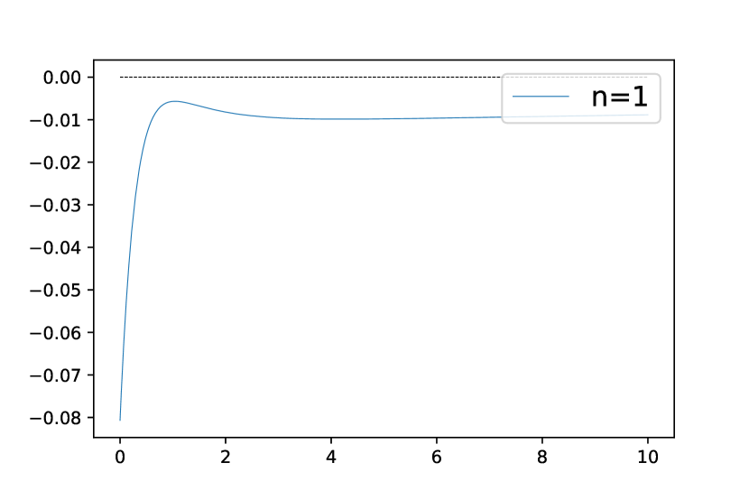
(a) Eigenvalues for $n=1$

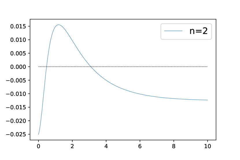
(b) Eigenvalues for $n=2$

Figure 1: Eigenvalues as functions of $\tau_{M}$ for $n=1$ and $n=2$

4.2 Critical curve

We investigate how the critical values depend on the parameters. For example, to examine the dependence on $\tau_{A}$, by plotting the points on the $\tau_{M}$-$\tau_{A}$ plane where the value of the eigenvalue (13) is zero, and we can draw a curve that divides the plane into stable and unstable areas. Here, the stable (unstable) area is the area where the homogeneous stationary solution is stable (unstable) for any pair of parameters $(\tau_{M},\tau_{A})$ in the region.

Figure 2 shows the critical curve in $\tau_{M}$-$\tau_{A}$ plane under $\mu=0.5$, $\eta=2.0$, and $\sigma=3.0$, and the frequency number is $n=3$. Here, $\Delta\tau_{A}\approx 0.0008$ and $\Delta\tau_{M}\approx 0.003$ are set. It can be seen from Figure 2 that when $\tau_{A}$ is sufficiently high, the two critical points $\tau_{M}^{*1}$ and $\tau_{M}^{*2}$ approach each other as $\tau_{A}$ increases, and eventually merge and then disappear.

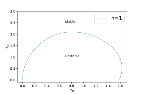
Figure 2: Critical curve for $\tau_{A}$ under $n=1$

Figure 3 shows the critical curves plotted for different frequencies $n$ under $\mu=0.5$, $\eta=2.0$, and $\sigma=3.0$. Here, $\Delta\tau_{A}\approx 0.0008$ and $\Delta\tau_{M}\approx 0.003$ are set. As can be seen from Figure 33(a), the unstable area does not necessarily expand monotonically outward as $n$ increases . However, this seems to be a minor part, and the unstable area tends to expand in terms of its size as $\tau_{M}^{*2}$ moves significantly to the right. Furthermore, especially if $n$ is limited to even or odd numbers, we would observe that the unstable area does not shrink at least inwardly as $n$ increases (Figure 33(b) and 33(c)). Thus, we would say that the unstable area generally expands with increasing $n$.

(a) For $n=1,2,3$

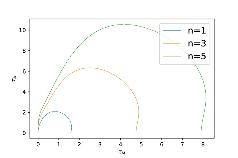
(b) For even numbers $n$

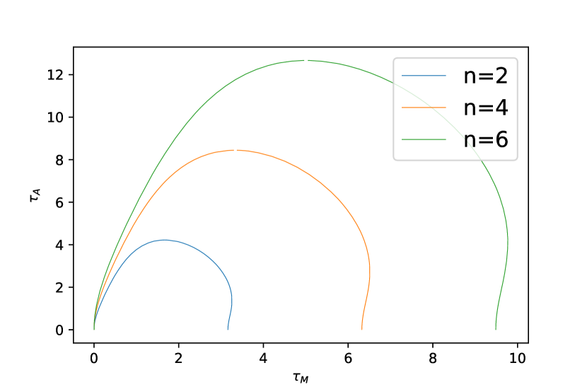
(c) For odd numbers $n$

Figure 3: Critical curve for $\tau_{A}$ under different frequencies

For the parameter $\eta>1$, the critical curves can be drawn in the $\tau_{M}$-$\eta$ plane. Figure 4 shows the critical curves on the $\tau_{M}$-$\eta$ plane for some frequencies under $\mu=0.5$, $\sigma=3.0$, and $\tau_{A}=2.5$. Here, $\Delta\eta\approx 0.002$ and $\Delta\tau_{M}\approx 0.003$ are set. We also observe that the unstable area would generally expand in its size as $n$ increases.

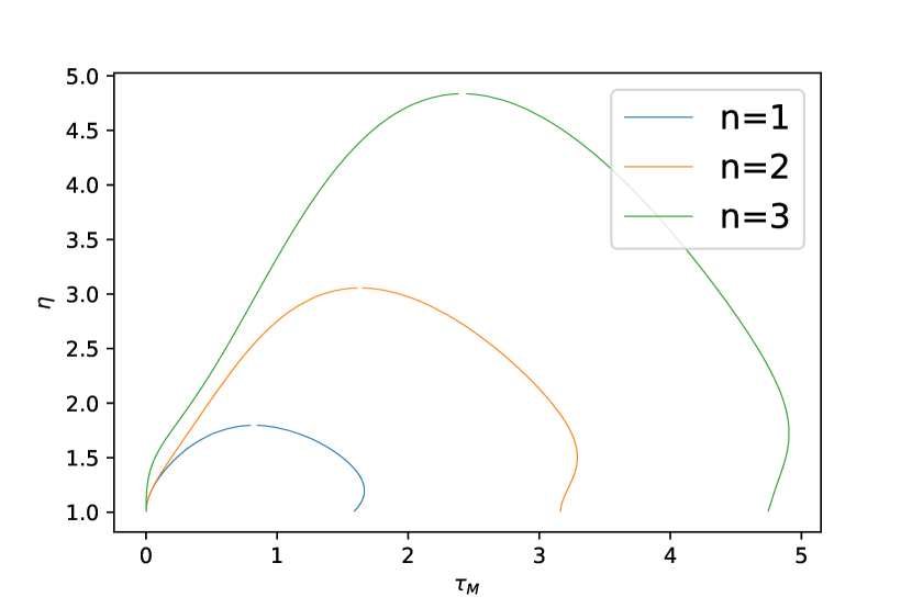
(a) For $n=1,2,3$

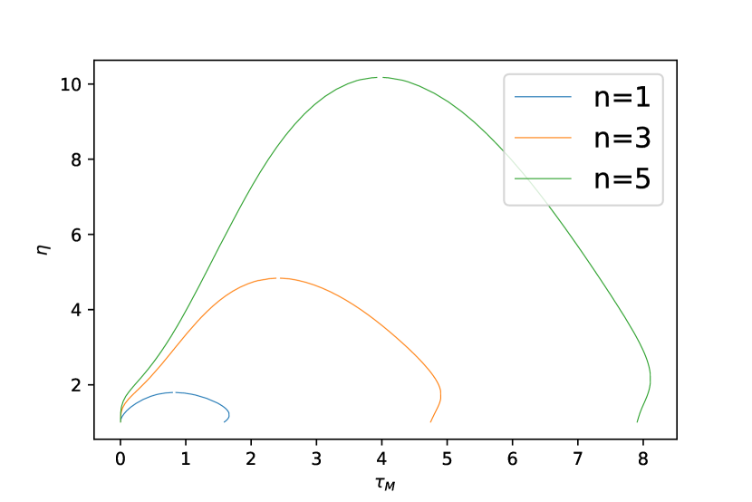
(b) For even numbers $n$

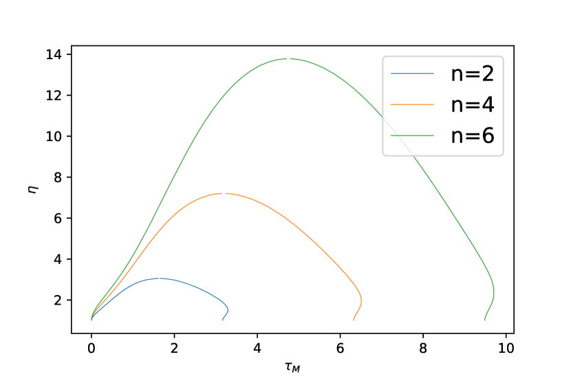
(c) For odd numbers $n$

Figure 4: Critical curve for $\eta$ under different frequencies

For the parameter $\sigma>1$, the critical curves for some frequencies under $\mu=0.5$, $\eta=2.0$, and $\tau_{A}=2.5$ are shown in Figure 5. Here, $\Delta\sigma\approx 0.03$ and $\Delta\tau_{M}\approx 0.01$ are set. The shape of the critical curve looks quite different from previous cases in Figure 3 and 4. However, we also observe that the unstable area would generally expand in its size as the frequency $n$ increases.

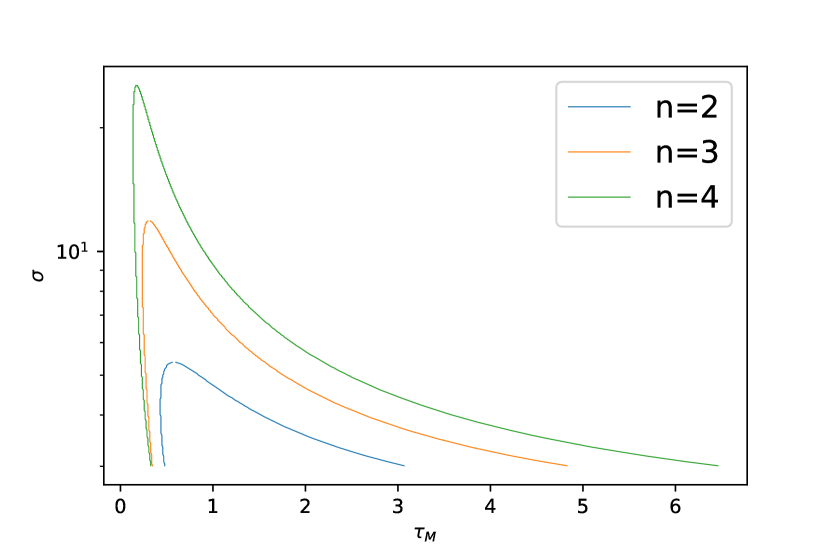
(a) For $n=2,3,4$

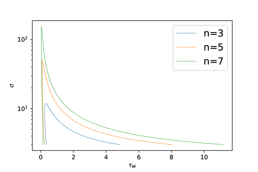
(b) For even numbers $n$

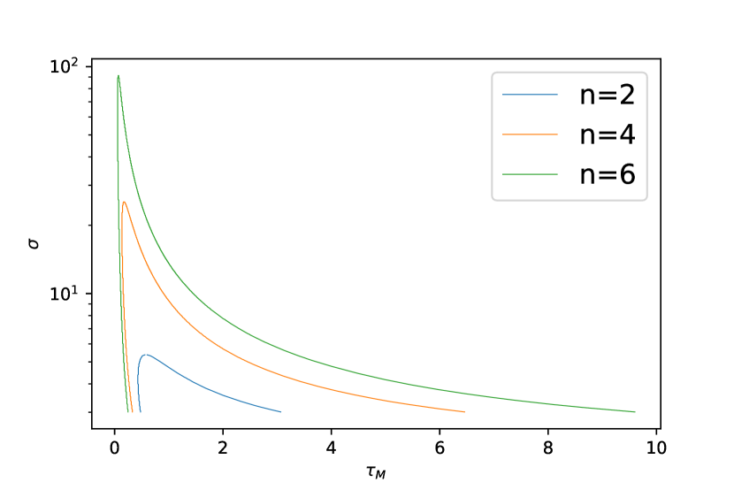
(c) For odd numbers $n$

Figure 5: Critical curve for $\sigma$ under different frequencies

Remark: Numerical observations alone would not provide absolute confirmation of the claim that the unstable area is truly “monotonically expanding outward as the frequency number increases while remaining even or odd”. This is not only because numerical observations are made only for a finite number of cases, but also because the critical curves corresponding to different frequencies can be so close to each other (especially on $\tau_{M}^{*1}$ side) that numerically they overlap exactly under some ranges of the parameters. For such cases, it would be impossible to infer the actual positional relationship of the critical curves, taking into account numerical errors.

5 Discussion and conclusion

We have considered a core-periphery model with differentiated agriculture and its transport cost on discrete and continuous multi-regional spaces. The stability of the homogeneous stationary solution of the model on a continuous periodic space has been investigated in detail.

By using Fourier analysis, we succeed in generalizing the results of the two-regional model by Fujita et al. (1999, Chapter 7) concerning the following points. First, each eigenfunction is found to behave similarly to the solution around the symmetric equilibrium of the two-regional model, i.e., it is stable at sufficiently high transport cost, unstable at moderate transport cost, and stable again at low transport cost. Second, the unstable area is found to expand generally as the frequency increases. This means that the eigenfunctions with high spatial frequencies are destabilized at very high and very low transport costs. That is, a dispersive spatial distribution of population is likely to be observed, similar to the two-regional model.

It may seem trivial, but the result not seen in the two-regional model also appears. That is, with the general increases in frequency $n$, it is observed that the unstable area does not necessarily expand uniformly outward, as seen in Figure 33(a). In particular, the fact that the lower critical point $\tau_{M}^{*1}$ can move to the right with increasing $n$ means that the economy can prefer to agglomerate into a relatively small number of regions rather than decentralize to a relatively large number of regions in a low range of the manufacturing transport cost. This is intuitively incompatible with the fact that the sufficiently low manufacturing transport cost makes the spatial structure more decentralized in the original two-regional model with differentiated agriculture (Fujita et al. (1999, p.110)). The author is not sure if an intuitive explanation of this phenomenon is possible, but it may reflect a richer spatial complexity than the two-regional model.

As noted in Remark to the previous section, our results rely on numerical observations. For a rigorous proof, it is necessary to compute analytically how the solution of the quadratic function as for $H^{\beta}_{n}$ in (9) behaves with respect to changes in frequency $n$ only within even numbers or only within odd numbers. However, there are difficulties that cannot be attributed to simple differential calculations.

6 Appendix

6.1 Modeling

This section provides an overview of the Dixit-Stiglitz framework (Dixit and Stiglitz (1977)) in the context of the differentiated agriculture with transport cost and applies it to derive the multi-regional version of the model which we handle.

6.1.1 Dixit-Stiglitz framework

The economy is supposed to have a continuously infinite variety of manufactured goods and agricultural goods. Let $m(i)\geq 0$ and $a(j)\geq 0$ denote demands for the variety $i\in[0,V_{M}]$ of the manufactured goods and the variety $j\in[0,V_{A}]$ of the agricultural goods. Price of $i$-th variety of the manufactured good is denoted by $p^{M}(i)$ and that of $j$-th variety of agricultural good is denoted by $p^{A}(j)$. Given an income $Y$, and the prices $p^{M}(i),p^{A}(j)$, each consumer faces the following budget constraint.

$$\int_{0}^{V_{M}}p^{M}(i)m(i)di+\int_{0}^{V_{A}}{p^{A}}(i)a(i)di=Y.$$ (16)

Facing (16), the consumer is supposed to maximize the following utility function.

$$M^{\mu}A^{1-\mu},~{}\mu\in(0,1),$$ (17)

where

$$M =\left[\int_{0}^{V_{M}}m(i)^{\frac{\sigma-1}{\sigma}}di\right]^{\frac{\sigma}{\sigma-1}}$$ (18)

$$A =\left[\int_{0}^{V_{A}}a(i)^{\frac{\eta-1}{\eta}}di\right]^{\frac{\eta}{\eta-1}}.$$ (19)

Following Fujita et al. (1999, Chapter 4), we solve this problem in two steps. First, the minimum cost to achieve the partial utility $M$ and $A$ is calculated, and then the optimal expenditure on $M$ and $A$ under the budget constraint is determined.

We obtain a function of consumer demand for the $j$-th variety of the agricultural goods as

$$a(j)=(1-\mu)Y{p^{A}_{j}}^{-\eta}{G^{A}}^{\eta-1},$$ (20)

where $Y$ is the income of the consumer, and $G^{A}$ is the price index of the agricultural goods defined by

$$G^{A}=\left[\int_{0}^{V_{A}}p^{A}(i)^{1-\eta}di\right]^{\frac{1}{1-\eta}}.$$ (21)

6.1.2 Multi-regional extension

Based on the framework described above, we model a two-sector spatial economy consisting of multiple regions. The modeling of manufacturing sector has already been described in detail in Fujita et al. (1999, Chapter 5 and 6), so we only mention it briefly. On the other hand, the agricultural sector is discussed in more detail here, since Fujita et al. (1999, Chapter 7) only mention the two-regional case.

In this subsection, the economy consists of $R$ discretely located regions indexed by $r$ or $s=1,2,\cdots R$. Following Fujita et al. (1999, Chapter 7), the total population of the mobile and immobile workers are normalized to be $\mu$ and $1-\mu$, respectively. Then, the mobile and immobile population in region $r$ is denoted by $\mu\lambda_{r}$ and $(1-\mu)\phi_{r}$, respectively. By these, it is easy to see that $\sum_{r=1}^{R}\lambda_{r}\equiv 1$ and $\sum_{r=1}^{R}\phi_{r}\equiv 1$.

Let $w_{r}^{M}$ and $w_{r}^{A}$ denote the nominal wage of the manufacturing and agricultural workers, respectively. Then, the total income of region $r$ is given by

$$Y_{r}=\mu w^{M}_{r}\lambda_{r}+(1-\mu)w^{A}_{r}\phi_{r}.$$ (22)

The prices of any variety of agricultural goods produced in region $r$ have equal value $p^{A}_{r}$. Assume that the transportation of the agricultural goods incurs the iceberg transport cost. That is, to transport one unit of agricultural goods from $r$ to $s$, $T^{A}_{rs}\geq 1$ times as much agricultural goods must be shipped. Then, the price in region $s$ of a variety of agricultural good produced in region $r$ is $p_{rs}^{A}=p^{A}_{r}T^{A}_{rs}$.

The number of varieties of agricultural goods produced in region $r$ denoted by $n^{A}_{r}$ is assumed to be proportional to the agricultural population in region $r$ as

$$n^{A}_{r}=\phi_{r},~{}r=1,2,\cdots,R.$$ (23)

This implies that the total number of varieties of agricultural goods in the economy is normalized to $1$.

Then from (21) and (23), the price index of the agricultural goods in $r$ is given by

$$G^{A}_{r} =\left[\sum_{s=0}^{R-1}\phi_{s}{p_{sr}^{A}}^{1-\eta}\right]^{\frac{1}{1-\eta}}.$$

By assuming $p^{A}_{r}=w^{A}_{r},~{}(\forall r)$, we obtain the following price index equation

$$G^{A}_{r}=\left[\sum_{s=1}^{R}\phi_{s}{w^{A}_{s}}^{1-\eta}{T^{A}_{rs}}^{1-\eta}\right]^{\frac{1}{1-\eta}}.$$ (24)

Let us derive the equation for the nominal wage of the agricultural workers. The demand for the $j$-th variety of agricultural goods by a consumer with income $Y$ is given by (20). Thus, the demand from region $s$ for one variety of agricultural good produced in region $r$ can be given as

$$(1-\mu)Y_{s}{p_{r}^{A}}^{-\eta}{T^{A}_{rs}}^{-\eta}{G^{A}_{s}}^{\eta-1}.$$ (25)

We obtain the sales of an agricultural producer in region $r$ as the following by adding up $T^{A}_{rs}$ times the amount in (25) over all regions.

$$q^{A}_{r}=(1-\mu){p^{A}_{r}}^{-\eta}\sum_{s=0}^{N-1}Y_{s}{T^{A}_{rs}}^{1-\eta}{G^{A}_{s}}^{\eta-1}.$$ (26)

Assume that the total supply of agricultural goods in region $r$ is equal to the population of the agricultural workers there given by $(1-\mu)\phi_{r}$. Since the number of varieties of the agricultural goods produced there is $n^{A}_{r}=\phi_{r}$ according to (23), the supply of one variety of the agricultural goods produced there is given by $(1-\mu)\phi_{r}/\phi_{r}=1-\mu$. Thus, the condition that the supply $1-\mu$ and demand (26) for each variety of the agricultural goods are equal, together with the assumption that $p^{A}_{r}=w^{A}_{r}$, yields

$$w^{A}_{r}=\left[\sum_{s=0}^{N-1}Y_{s}{G^{A}_{s}}^{\eta-1}{T^{A}_{rs}}^{1-\eta}\right]^{\frac{1}{\eta}}.$$ (27)

For the price index $G^{M}_{r}$ and nominal wage $w^{M}_{r}$ in the manufacturing sector, exactly the same equations are derived as in the one-sector racetrack model (See (5.4) and (5.5) of Fujita et al. (1999, p.63)). That is

$$G^{M}_{r}=\left[\sum_{s=0}^{N-1}\lambda_{s}{w^{M}_{s}}^{1-\sigma}e^{-\tau_{M}(\sigma-1)|r-s|}\right]^{\frac{1}{1-\sigma}}$$ (28)

and

$$w^{M}_{r}=\left[\sum_{s=0}^{N-1}Y_{s}{G^{M}_{s}}^{\sigma-1}e^{-\tau_{M}(\sigma-1)|r-s|}\right]^{\frac{1}{\sigma}}.$$ (29)

As mentioned in Fujita et al. (1999, Chapter 7), the real wage of the mobile workers is

$$\omega_{r}=w^{M}_{r}{G^{M}_{r}}^{-\mu}{G^{A}_{r}}^{\mu-1}.$$ (30)

We adopt the following ad-hoc dynamics in which the mobile workers flow into regions with above-average real wage, while they flow out of regions with below-average real wage. The average real wage is defined by $\sum_{s=1}^{R}\omega_{s}\lambda_{s}$ and the dynamics is described by

$$\frac{\partial}{\partial t}\lambda_{r}=\gamma\left[\omega_{r}-\sum_{s=1}^{R}\omega_{s}\lambda_{s}\right]\lambda_{r},$$ (31)

where $\gamma>0$ stands for adjustment speed.

The equations (22), (24), (27), (28), (29), (30), and (31) constitute the following system of nonlinear algebraic differential equations.

$$\left\{\begin{aligned} &Y_{r}(t)=\mu w^{M}_{r}(t)\lambda_{r}(t)+(1-\mu)w^{A}_{r}(t)\phi_{r},\\ &G^{A}_{r}(t)=\left[\sum_{s=1}^{R}\phi_{s}{w^{A}_{s}(t)}^{1-\eta}{T^{A}_{rs}}^{1-\eta}\right]^{\frac{1}{1-\eta}},\\ &w^{A}_{r}(t)=\left[\sum_{s=1}^{R}Y_{s}(t){G^{A}_{s}(t)}^{\eta-1}{T^{A}_{rs}}^{1-\eta}\right]^{\frac{1}{\eta}},\\ &G^{M}_{r}(t)=\left[\sum_{s=1}^{R}\lambda_{s}(t){w^{M}_{s}(t)}^{1-\sigma}{T^{M}_{rs}}^{1-\sigma}\right]^{\frac{1}{1-\sigma}},\\ &w^{M}_{r}(t)=\left[\sum_{s=1}^{R}Y_{s}(t){G^{M}_{s}(t)}^{\sigma-1}{T^{M}_{rs}}^{1-\sigma}\right]^{\frac{1}{\sigma}},\\ &\omega_{r}(t)=w^{M}_{r}(t){G^{M}_{r}(t)}^{-\mu}{G^{A}_{r}(t)}^{\mu-1},\\ &\frac{\partial}{\partial t}\lambda_{r}(t)=\gamma\left[\omega_{r}(t)-\sum_{s=1}^{R}\omega_{s}(t)\lambda_{s}(t)\right]\lambda_{r}(t)\end{aligned}\right.$$ (32)

with an initial condition $\lambda_{r}(0)=\lambda_{0,r}\geq 0,~{}(r=1,2,\cdots,R)$ which satisfies $\sum_{r=1}^{R}\lambda_{0,r}=1$.

Then, if we consider the system (32) in continuous space, with the population here being the population density, we naturally obtain (1).

6.2 Proofs

Proof for Lemma 1

When $n$ is even

In this case, we see

$$H^{\beta}_{n}=\frac{\beta^{2}r^{2}}{n^{2}+\beta^{2}r^{2}}.$$

Putting $\beta r=X$, we have

$$H^{\beta}_{n}=\frac{X^{2}}{n^{2}+X^{2}}.$$

It is easy to see that

$$\lim_{X\to 0}\frac{X^{2}}{n^{2}+X^{2}}=0,$$

$$\lim_{X\to\infty}\frac{X^{2}}{n^{2}+X^{2}}=1.$$

We also easily see that

$$\frac{d}{dX}H^{\beta}_{n}=\frac{2n^{2}X}{(n^{2}+X^{2})^{2}}>0.$$

When $n$ is odd

In this case, we see

$$H^{\beta}_{n}=\frac{X^{2}(1+e^{-X\pi})}{(n^{2}+X^{2})(1-e^{-X\pi})}$$

by putting $X=\beta r$. By the L’Hopital’s theorem, we have

$$\lim_{X\to 0}H^{\beta}_{n}=\lim_{X\to 0}\frac{2X(1+e^{-\pi X})+X^{2}(-\pi e^{-\pi X})}{2X(1-e^{-\pi X})+(n^{2}+X^{2})\pi e^{-\pi X}}=0.$$

On the other hand, it is obvious that

$$\lim_{X\to\infty}H^{\beta}_{n}=1.$$

By differentiating $H^{\beta}_{n}$ by $X$, we obtain

$$\frac{d}{dX}H^{\beta}_{n}=\frac{2n^{2}X(1-e^{-2\pi X})-2\pi X^{2}e^{-\pi X}(n^{2}+X^{2})}{(n^{2}+X^{2})^{2}(1-e^{-\pi X})^{2}}.$$ (33)

To show the monotonicity of $H^{\beta}_{n}$ as for $X$, we need to prove that the numerator of (33) is positive. It is equivalent to

$$e^{\pi X}-e^{-\pi X}>\frac{\pi X}{n^{2}}(n^{2}+X^{2}).$$ (34)

The left hand side of (34) is expanded into a series

$$2\pi X+2\frac{(\pi X)^{3}}{3!}+2\frac{(\pi X)^{5}}{5!}+\cdots.$$

Therefore, subtracting the right-hand side of (34) from the left-hand side of (34) yields

$$\pi X+\left\{2\frac{(\pi X)^{3}}{3!}-\frac{\pi}{n^{2}}X^{3}\right\}+2\frac{(\pi X)^{5}}{5!}+\cdots.$$ (35)

We are left with the task of proving the content of the braces in (35) is positive. It is sufficient to prove for $n=1$, and it is obvious that

$$\pi\left(\frac{\pi^{2}}{3}-1\right)X^{3}>0.$$

∎

Proof for Lemma 2

It is easy to check that

$$\frac{d}{dH^{\alpha}_{n}}b=-(1-\mu)\frac{\eta+(\eta-1){H^{\alpha}_{n}}^{2}}{\left[\eta-(\eta-1){H^{\alpha}_{n}}^{2}\right]^{2}}<0.$$

It is also immediate that

$$b=1$$

for $\alpha=0$ because $\alpha=0\Leftrightarrow H^{\alpha}_{n}=0$, and

$$\lim_{H^{\alpha}_{n}\to 1}b=1-\frac{1-\mu}{\eta-(\eta-1)}=\mu.$$

∎

Proof for Lemma 3

It is evident from (11) and Lemma 2. ∎

Proof for Theorem 1

When the manufacturing transport cost goes to infinity, i.e., when $\beta$ goes to infinity, the content in the square brackets of (9) becomes

$$1+\frac{-\sigma\mu^{2}-\sigma b+\mu\sigma b+\mu\sigma-\mu}{b}.$$ (36)

For there to be no black hole, (36) must be negative, for which it is sufficient that

$$(1-\sigma+\mu\sigma)(b-\mu)<0.$$

Since $b\in(\mu,1]$ from Lemma 2, it immediately yields (14).

∎

Proof for Theorem 2

When $\tau_{M}\to 0$ or $\sigma\to 1$, i.e., $\beta\to 0$, we see that $H^{\beta}_{n}\to 0$ by Lemma 1. Then, it is easy to see $D\to\sigma$ by (12). As a result, it immediately follows from (13) that

$$\Omega_{n}\to-\frac{2\pi r\overline{\omega}}{(\sigma-1)\sigma}B.$$

For $\alpha>0$, it is obvious that this limit is negative since $B>0$ from Lemma 3.

∎

References

- (1)
- Deaton and Muellbauer (1980) Deaton, A. and J. Muellbauer, Economics and Consumer Behavior, Cambridge University Press, 1980.
- Dixit and Stiglitz (1977) Dixit, A. K. and J. E. Stiglitz, “Monopolistic competition and optimum product diversity,” A. E. R., 1977, 67 (3), 297–308.
- Fujita et al. (1999) Fujita, M., P. Krugman, and A. Venables, The Spatial Economy: Cities, Regions, and International Trade, MIT Press, 1999.
- Gallego and Zofío (2018) Gallego, Nuria and José L Zofío, “Trade openness, transport networks and the spatial location of economic activity,” Networks and Spatial Economics, 2018, 18, 205–236.
- Green (1964) Green, H. A. John, Aggregation in Economic Analysis, Princeton University Press, 1964.
- Krugman (1991) Krugman, P., “Increasing returns and economic geography,” J. Polit. Econ., 1991, 99 (3), 483–499.
- Ottaviano and Thisse (2004) Ottaviano, Gianmarco and Jacques-François Thisse, “Agglomeration and economic geography,” in “Handbook of Regional and Urban Economics,” Vol. 4 2004, pp. 2563–2608.
- Picard and Zeng (2005) Picard, P. M. and D.-Z. Zeng, “Agricultural sector and industrial agglomeration,” J. Dev. Econ., 2005, 77 (1), 75–106.
- Samuelson (1952) Samuelson, P. A., “The transfer problem and transport costs: the terms of trade when impediments are absent,” Econ. J., 1952, 62 (246), 278–304.
- Takatsuka and Zeng (2012) Takatsuka, H. and D.-Z. Zeng, “Trade liberalization and welfare: Differentiated-good versus homogeneous-good markets,” J. Jpn. Int. Econ., 2012, 26 (3), 308–325.
- Zeng (2021) Zeng, D.-Z., “Spatial economics and nonmanufacturing sectors,” Interdiscip. Inf. Sci., 2021, 27 (1), 57–91.
- Zeng and Kikuchi (2009) and T. Kikuchi, “Home market effect and trade costs,” Jpn. Econ. Rev., 2009, 60 (2), 253–270.
- Zeng and Takatsuka (2016) and H. Takatsuka, Spatial Economics (in Japanese), TOYO KEIZAI INC., 2016.