Primordial black holes and scalar-induced gravitational waves from the generalized Brans-Dicke theory

Abstract

The power spectrum of the scalar-tensor inflation with a quadratic form Ricci scalar coupling function $\Omega(\phi)=1-2\phi/\phi_{c}+(1+\delta^{2})(\phi/\phi_{c})^{2}$ can be enhanced enough to produce primordial black holes and generate scalar-induced gravitational waves. The masses of primordial black holes and the frequencies of scalar-induced gravitational waves are controlled by the parameter $\phi_{c}$, and their amplitudes are determined by the parameter $\delta$. Primordial black holes with stellar masses, planetary masses, and masses around $10^{-12}M_{\odot}$ are produced and their abundances are obtained from the peak theory. The frequencies of the corresponding scalar-induced gravitational waves are around $10^{-9}$ Hz, $10^{-6}$ Hz, and $10^{-3}$ Hz, respectively. The primordial black holes with masses around $10^{-12}M_{\odot}$ can account for almost all of the dark matter, and the scalar-induced gravitational waves with frequencies around $10^{-9}$ Hz can explain the NANOGrav 12.5yrs signal.

1 Introduction

Primordial black holes (PBHs) can be formed from the gravitational collapse of overdense regions with their density contrasts exceeding the threshold value at the horizon reentry during radiation domination [1, 2]. PBHs with stellar masses may be the black holes in the gravitational waves (GWs) events detected by the Laser Interferometer Gravitational Wave Observatory (LIGO) Scientific Collaboration and the Virgo Collaboration [3, 4, 5, 6, 7, 8, 9, 10, 11, 12, 13, 14, 15, 16]. PBHs with planetary masses can explain the ultrashort-timescale microlensing events in the OGLE data [17], and can act as the Planet 9 which is a hypothetical astrophysical object in the outer solar system used to explain the anomalous orbits of trans-Neptunian objects [18]. PBHs are also proposed to account for dark matter (DM) [19, 20, 21, 22, 23, 24, 25, 26, 27], and those with masses around $10^{-17}-10^{-15}M_{\odot}$ and $10^{-14}-10^{-12}M_{\odot}$ can make up almost all of DM for there are no observational constraints on the abundances of PBHs at these mass windows.

The overdense regions, collapsing to PBHs by gravitational force, originate from the primordial curvature perturbations generated during Inflation. From the threshold value of the density contrasts for PBHs formation, the amplitude of the power spectrum of the primordial curvature perturbations is constrained to $A_{\zeta}\sim\mathcal{O}(0.01)$, which is seven orders of magnitude larger [28, 29, 30] than the large scale constraints $A_{\zeta}=2.1\times 10^{-9}$ [31] from the observation of cosmic microwave background (CMB) anisotropy measurements. Therefore, the allowed way to produce enough PBHs DM is by enhancing the power spectrum by about seven orders of magnitude at small scales.

The traditional slow-roll inflation model is hard to enhance the power spectrum at small scales while keeping the model consistent with the large scale constraints. To solve this difficult, we need consider the ultra-slow-roll inflation model that transiently satisfies the condition $\ddot{\phi}+3H\dot{\phi}\approx 0$ [32, 33, 34]. For the canonical inflation models with a single field, a simple way to realize the ultra-slow-roll inflation is by introducing an inflection point in the potential [35, 36, 37, 38, 28, 39, 40, 41, 42]. However, it is not easy to achieve the big enhancement on the power spectrum while keeping the total number of e-folds around $50-60$ [43, 44]. Noncanonical kinetic terms inflation [45, 46, 47, 48, 49, 50, 51, 52, 53] or other kinds of noncanonical inflation models [54, 55, 56, 57, 58, 59, 60, 61, 62, 63, 64, 65, 66, 67] were then considered. For example, with the coupling function $f(\phi)$ and potential satisfying $(V_{\phi}+V^{2}f_{\phi}/6)|_{\phi=\phi_{c}}\approx 0$, the Gauss-Bonnet inflation model has a transient ultra-slow-roll process at the critical point $\phi_{c}$ [60, 61] and succeeds in enhancing the power spectrum and produce PBHs. The noncanonical kinetic term inflation model with coupling function $G(\phi)=h/[1+\left(|\phi-\phi_{c}|/{w}\right)^{q}]$ can realize a large enhancement on the power spectrum and produce PBHs if the parameter $h$ is large enough [45, 50]. Besides the noncanonical single field inflation models, the multi-filed inflationary models are another important way to enhance the power spectrum [68, 69, 70], especially those with tachyonic instabilities [71, 72, 73]. In this paper, we focus on the scalar-tensor inflation and find that with the Ricci scalar coupling function being a quadratic form $\Omega(\phi)=1-2\phi/\phi_{c}+(1+\delta^{2})(\phi/\phi_{c})^{2}$, the ultra-slow-roll condition can be satisfied transiently at the critical point $\phi_{c}$, and the power spectrum can be enhanced enough to produce PBHs. The masses and abundances of the PBHs can be adjusted by the parameters $\phi_{c}$ and $\delta$, respectively. It was pointed out recently that a single field inflation model, producing an appreciable amount of PBHs, is in danger of excessive one-loop corrections to the CMB scale [74]. Hence, our model is potentially in danger of the one-loop effect, but it is beyond the scope of the present paper and left for future study.

With the formation of PBHs, the large scalar perturbations at small scales induce secondary gravitational waves after the horizon reentry during the radiation dominated epoch [75, 76, 77, 78, 79, 80, 81, 82, 83, 84, 85, 86, 87, 88, 89, 90, 91, 92, 93, 94, 95, 96, 97, 98, 99, 100, 101, 102, 103, 104, 105, 106, 107, 108, 109, 110, 111, 112, 113, 114]. These scalar-induced gravitational waves (SIGWs) have wide frequency distribution and can be detected by pulsar timing arrays (PTA) [115, 116, 117, 118, 119] and the space-based GW detectors such as Laser Interferometer Space Antenna (LISA) [120, 121], Taiji [122], TianQin [123] and Deci-hertz Interferometer Gravitational Wave Observatory (DECIGO) [124] in the future. For example, the stochastic process with a common amplitude and a common spectral slope across pulsars detected by the North American Nanohertz Observatory for Gravitational Wave (NANOGrav) Collaboration [125] and other pulsar timing arrays [126, 127] recently may be the SIGWs with nHz frequencies[128, 129, 130, 131, 51, 132].

The paper is organized as follows. In Sec. II, we show the enhancement mechanism on the power spectrum of the scalar-tensor inflation in detail. We discuss the production of PBH DM and the generation of SIGWs from this mechanism in Sec. III. We conclude the paper in Sec. V.

2 The model

The action for the scalar-tensor theory in the Jordan frame is

$$S=\int\sqrt{-g}dx^{4}\left[\frac{\Omega(\phi)}{2}R-\frac{\omega(\phi)}{2}(\partial\phi)^{2}-V(\phi)\right],$$ (2.1)

where $\Omega(\phi)$ and $\omega(\phi)$ are the coupling functions, and $V(\phi)$ is the potential, $(\partial\phi)^{2}=g^{\mu\nu}\nabla_{\mu}\phi\nabla_{\nu}\phi$. The reduced Planck mass is $M_{\rm pl}=1/\sqrt{8\pi G}$, and the units are $c=\hbar=M_{\rm pl}=1$. For the homogeneous and isotropic background, the Friedmann equation and the equation of motion for the scalar field are

$$H^{2}=\frac{1}{3\Omega}\left(\frac{1}{2}\omega\dot{\phi}^{2}+V\right)-H\frac{\dot{\Omega}}{\Omega},$$ (2.2)

$$\left[\omega+\frac{3}{2\Omega}\left(\frac{d\Omega}{d\phi}\right)^{2}\right](\ddot{\phi}+3H\dot{\phi})+\frac{dV}{d\phi}-\frac{2V}{\Omega}\frac{d\Omega}{d\phi}$$ (2.3)

$$\quad+\left(\frac{3}{2\Omega}\frac{d\Omega}{d\phi}\frac{d^{2}\Omega}{d\phi^{2}}+\frac{1}{2}\frac{d\omega}{d\phi}+\frac{1}{\Omega}\frac{d\Omega}{d\phi}\frac{w}{2}\right)\dot{\phi}^{2}=0,$$

where a “dot” denotes the derivative with respect to cosmic time $t$. Under the slow-roll conditions [133]

$$\frac{1}{2}\omega(\phi)\dot{\phi}^{2}\ll V(\phi),\quad|\dot{g}|\ll Hg,$$ (2.4)

where the function $g$ denotes an arbitrary function, such as $\Omega(\phi)$ and $\omega(\phi)$, the background equations (2.2) and (2.3) become

$$H^{2}\approx\frac{V(\phi)}{3\Omega(\phi)},$$ (2.5)

$$(\ddot{\phi}+3H\dot{\phi})+\Gamma(\phi)\frac{dU(\phi)}{d\phi}\approx 0,$$ (2.6)

with the effective potential $U(\phi)=V(\phi)/\Omega(\phi)^{2}$ and

$$\Gamma(\phi)=\frac{\Omega(\phi)^{2}}{\omega(\phi)+\frac{3}{2\Omega}\left(\frac{d\Omega}{d\phi}\right)^{2}}.$$ (2.7)

The condition of forming PBHs requires the amplitude of the power spectrum of the primordial curvature to reach around $A_{\zeta}\sim\mathcal{O}(0.01)$, while the constraints on power spectrum at large scales from the observation of CMB anisotropy measurements is $A_{\zeta}=2.1\times 10^{-9}$ [134]. Therefore, to produce PBHs, the power spectrum should be enhanced by about seven orders of magnitude at small scales, and this is hard to realize in the slow-roll inflation model. For the ultra-slow-roll inflation with condition [32]

$$\ddot{\phi}+3H\dot{\phi}\approx 0,$$ (2.8)

the power spectrum can be enhanced enough to produce PBHs. From equation (2.6), to obtain the ultra-slow-roll condition (2.8), we need

$$\Gamma(\phi)\frac{dU(\phi)}{d\phi}\ll 1.$$ (2.9)

If the effective potential $U(\phi)$ has a near inflection point, $dU(\phi)/d\phi|_{\phi=\phi_{c}}\approx 0$, the condition (2.9) can be satisfied easily [35, 28]. In addition to the method of near inflection point, the other way to obtain condition (2.9) is by making the coupling functions satisfy

$$\Gamma(\phi)=\frac{\Omega(\phi)^{2}}{\omega(\phi)+\frac{3}{2\Omega}\left(\frac{d\Omega}{d\phi}\right)^{2}}\ll 1,$$ (2.10)

which requires $\omega(\phi)\gg 1$ or $\Omega(\phi)\ll 1$ at the ultra-slow-roll point. The situation $\omega(\phi)\gg 1$ has been researched in papers [45, 50] with the form

$$\omega(\phi)=1+\frac{h}{1+\left(|\phi-\phi_{c}|/{w}\right)^{q}},$$ (2.11)

and $h\gg 1$. At the point $\phi_{c}$, the coupling function satisfies $\omega(\phi_{c})=1+h\gg 1$, and the ultra-slow-roll condition (2.10) is satisfied.

In this paper, we consider the other case, $\Omega(\phi)\ll 1$. Inspired by the Higgs inflation [135] with the coupling function $\Omega(\phi)=1+\xi\phi^{2}$, we consider the second-order polynomial

$$\Omega(\phi)=1-\frac{2\phi}{\phi_{c}}+(1+\delta^{2})\left(\frac{\phi}{\phi_{c}}\right)^{2},$$ (2.12)

where the term $\delta^{2}\ll 1$ is used to keep the coupling function $\Omega(\phi)$ from exact zero. At the critical point, the coupling function becomes $\Omega(\phi_{c})=\delta^{2}\ll 1$, the condition (2.10) is satisfied, the inflaton evolves into a transitory ultra-slow-roll phase where the power spectrum of the curvature perturbations is enhanced. The critical point $\phi_{c}$ controls the position of the peak in the power spectrum and $\delta$ determines the amplitude of the peak. The choice (2.12) may be the simplest form containing a critical point satisfying condition $\Omega(\phi_{c})\ll 1$, and this choice could be regarded as a phenomenological step, and finding the corresponding UV theory will be the next step.

To obtain the condition (2.10), even if the numerator of relation (2.10) is chosen as equation (2.12) and satisfies $\Omega(\phi_{c})\ll 1$, the denominator should satisfy

$$\omega(\phi_{c})+\frac{3}{2\Omega(\phi_{c})}\left(\frac{d\Omega(\phi_{c})}{d\phi}\right)^{2}\gtrsim\Omega(\phi_{c})^{p},$$ (2.13)

at the critical point with $p<2$. In order to satisfy condition (2.13), we choose the kinetic coupling function as

$$\omega(\phi)+\frac{3}{2\Omega(\phi)}\left(\frac{d\Omega(\phi)}{d\phi}\right)^{2}=a\Omega(\phi)^{b}+c\Omega(\phi),$$ (2.14)

with $b<1$, and the form of $\omega(\phi)$ can be obtained completely by that of $\Omega(\phi)$. The first term $a\Omega(\phi)^{b}$ is used to adjust the shape of the peak, and the second term $c\Omega(\phi)$ is used to keep $w(\phi)=1$ at the lower energy scales $\phi\ll 1$, which requires

$$c=1-a+\frac{6}{\phi_{c}^{2}}.$$ (2.15)

The abilities to produce different peaks in the primordial power spectrum as displayed in figure 1 and recover to the canonical situation at the lower energy are the main reason to choose form (2.14), although it is not conventional.

The potential is [46]

$$V(\phi)=\frac{\lambda\phi^{4}}{4}\left(\frac{\Omega(\phi)}{1+\xi\phi^{2}}\right)^{2},$$ (2.16)

with $\xi=10$. At the lower energy scales $\phi\ll 1$, the potential reduces to the Higgs potential with the form $\lambda\phi^{4}/4$.

In the other hand, taking the conformal transformation,

$$\tilde{g}_{\mu\nu}=\Omega(\phi)g_{\mu\nu},$$ (2.17)

and changing the Jordan frame to the Einstein frame, action (2.1) becomes

$$S=\int d^{4}x\sqrt{-\tilde{g}}\left[\frac{\tilde{R}}{2}-\frac{1}{2}k(\phi)(\tilde{\partial}\phi)^{2}-\frac{V(\phi)}{\Omega(\phi)^{2}}\right],$$ (2.18)

with $(\tilde{\partial}\phi)^{2}=\tilde{g}^{\mu\nu}\nabla_{\mu}\phi\nabla_{\nu}\phi$ and

$$k(\phi)=\frac{3}{2}\left(\frac{d\Omega/d\phi}{\Omega}\right)^{2}+\frac{\omega(\phi)}{\Omega(\phi)}.$$ (2.19)

Combining equation (2.12) and (2.14), the coupling function of the kinetic term becomes

$$k(\phi)=1+\left(-a+\frac{6}{\phi_{c}^{2}}\right)+\frac{a}{\Omega^{1-b}}=1+G(\phi)$$ (2.20)

with

$$G(\phi)=\left(\frac{6}{\phi_{c}^{2}}-a\right)+\frac{a(\phi_{c}/\delta)^{2-2b}}{\left[\left(\frac{\phi-\phi_{c}}{\delta}\right)^{2}+\phi^{2}\right]^{1-b}},$$ (2.21)

which is similar with equation (2.11). As pointed out in Refs. [45, 50], this kind of kinetic term can succeed in enhancing the power spectrum and producing enough PBHs.

3 The results

3.1 power spectra

The quadratic action for the curvature perturbation $\zeta$ of the scalar-tensor inflation (2.1) is

$$S^{(2)}=\frac{1}{2}\int d\eta d^{3}x\frac{a^{2}[\omega\dot{\phi}^{2}+3\dot{\Omega}^{2}/2\Omega]}{(H+\dot{\Omega}/2\Omega)^{2}}\left[(\zeta^{\prime})^{2}-(\vec{\nabla}\zeta)^{2}\right],$$ (3.1)

where $\eta=\int dt/a$ is the conformal time and $\zeta^{\prime}=d\zeta/d\eta$. The equation for the curvature perturbation in $k$-space is

$$\frac{d^{2}u_{k}}{d\eta^{2}}+\left(k^{2}-\frac{1}{z}\frac{d^{2}z}{d\eta^{2}}\right)u_{k}=0,$$ (3.2)

with $u_{k}=z\zeta_{k}$ and [136]

$$z^{2}=\frac{a^{2}[\omega\dot{\phi}^{2}+3\dot{\Omega}^{2}/2\Omega]}{(H+\dot{\Omega}/2\Omega)^{2}}.$$ (3.3)

The power spectrum of the curvature perturbation is

$$\mathcal{P}_{\zeta}=\frac{k^{3}}{2\pi^{2}}\left|\zeta_{k}\right|^{2},$$ (3.4)

which can be obtain by solving the background equations (2.2) and (2.3), and the perturbation equation (3.2).

By choosing the values of parameters $a$, $\delta$, $\phi_{c}$, $\lambda$, and the scalar field $\phi_{*}$ at the pivot scale, we can numerically obtain the power spectrum. For the values of the parameter sets listed in table 1, the numerical results of the power spectra of the curvature perturbation are shown in figure 1. The $e$-folding numbers $N$ of these models in table 1 are about $N\in(55,65)$. The scalar tilt and tensor-to-scalar ratio of these models are listed in table 1 which are around

$$n_{s}\approx 0.965,\quad r\approx 0.004,$$ (3.5)

which are consistent with the observational constraints [31, 137],

$$n_{s}=0.9649\pm 0.0042\quad(68\%\,\text{CL}),$$ (3.6)

$$r_{0.05}<0.06\quad(95\%\,\text{CL}).$$ (3.7)

The position of the peak of the power spectra in figure 1 is controlled by the parameter $\phi_{c}$ in equation (2.12). The power spectra with peak scale around $k_{\text{peak}}\approx 10^{6}\,\text{Mpc}^{-1}$, $k_{\text{peak}}\approx 10^{9}\,\text{Mpc}^{-1}$, and $k_{\text{peak}}\approx 10^{12}\,\text{Mpc}^{-1}$ are given in figure 1, and denoted as red lines, green lines, and black lines, respectively. In table 1, they are labeled as “1”, “2”, and “3”, respectively. The shape of the peak is determined by the index $b$ in equation (2.14). The narrow peak denoted by the dashed line in figure 1 is from the model with $b=1/2$ and labeled as “Mn” in table 1, the broad peak denoted by the solid line in figure 1 is from the model with $b=2/5$ and labeled as “Mb” in table 1.

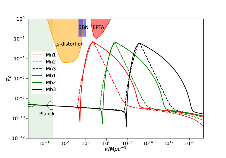
Figure 1: The power spectra of the models listed in table 1. The light green shaded region is excluded by the CMB observations [134]. The red, blue and orange regions are the constraints from the PTA observations [138], the effect on the ratio between neutron and proton during the big bang nucleosynthesis (BBN) [139] and $\mu$-distortion of CMB [140], respectively.

Model	$a$	$\delta$	$\phi_{c}$	$\phi_{*}$	$\lambda/10^{-8}$	$N$	$n_{s}$	$r/10^{-3}$	$k_{\text{peak}}/\text{Mpc}^{-1}$
Mn1	$1.53\times 10^{-2}$	$1.10\times 10^{-9}$	$1.96$	$2.13$	$6.02$	$54$	$0.964$	$4.6$	$1.08\times 10^{6}$
Mn2	$1.95\times 10^{-2}$	$2.73\times 10^{-10}$	$1.83$	$2.13$	$5.67$	$57$	$0.963$	$4.4$	$1.52\times 10^{9}$
Mn3	$2.66\times 10^{-2}$	$7.93\times 10^{-11}$	$1.69$	$2.13$	$5.16$	$61$	$0.966$	$4.0$	$5.75\times 10^{12}$
Mb1	$1.50\times 10^{-3}$	$3.18\times 10^{-11}$	$2.03$	$2.25$	$4.77$	$60$	$0.965$	$3.7$	$1.26\times 10^{6}$
Mb2	$2.46\times 10^{-3}$	$1.19\times 10^{-10}$	$1.82$	$2.18$	$5.05$	$61$	$0.965$	$3.9$	$2.36\times 10^{9}$
Mb3	$4.24\times 10^{-3}$	$4.67\times 10^{-11}$	$1.61$	$2.12$	$5.07$	$65$	$0.966$	$3.9$	$6.31\times 10^{12}$

Table 1: The chosen parameter sets and the predictions of scalar tilt $n_{s}$, tensor-to-scalar ratio $r$, and $e$-folds $N$.

3.2 primordial black holes

If the amplitude of the power spectrum is enhanced to $A_{\zeta}\sim\mathcal{O}(0.01)$ at small scales, it may form PBHs from gravitational collapse during the radiation domination. The mass fraction of the Universe that collapses to form PBHs at formation is denoted by

$$\beta=\frac{\rho_{\text{PBH}}}{\rho_{b}},$$ (3.8)

where $\rho_{b}$ is the energy density of the background and $\rho_{\text{PBH}}$ is the energy density of the PBHs at formation. From the peak theory, the energy density of the PBHs is [141, 142, 143, 144, 145, 146],

$$\rho_{\text{PBH}}=\int_{\nu_{c}}^{\infty}M_{\text{PBH}}(\nu)\mathcal{N}_{pk}(\nu)d\nu,$$ (3.9)

where the number density of the PBHs is [141]

$$\mathcal{N}_{pk}(\nu)=\frac{1}{a^{3}}\frac{1}{(2\pi)^{2}}\left(\frac{\sigma_{1}}{\sqrt{3}\sigma_{0}}\right)^{3}\nu^{3}\exp\left(-\frac{\nu^{2}}{2}\right).$$ (3.10)

The lower limit of the integral in equation (3.9) is $\nu_{c}=\delta_{c}/\sigma_{0}$, $\delta_{c}$ is the threshold for the formation of PBHs, and $\sigma_{0}$ is the variance of the smoothed density contrast. The moment of the smoothed density power spectrum $\sigma_{1}$ is defined by

$$\sigma^{2}_{n}=\int_{0}^{\infty}\frac{dk}{k}k^{2n}T^{2}(k,R_{H})W^{2}(k,R_{H})\mathcal{P}_{\delta}(k),$$ (3.11)

where $\mathcal{P}_{\delta}$ is the power spectrum of the density contrast which is related to the power spectrum of primordial curvature perturbations $\mathcal{P}_{\zeta}$ by

$$\mathcal{P}_{\delta}(k)=\frac{4(1+w)^{2}}{(5+3w)^{2}}\left(\frac{k}{aH}\right)^{4}\mathcal{P}_{\zeta}(k),$$ (3.12)

with the state equation $w=1/3$ during the radiation domination.

For the window function $W(k,R_{H})$ in equation (3.11), there are usual three choices, the real-space top-hat window function, the Gauss window function, and the $k$-space top-hat window function [147]. In this paper, we choose the real-space top-hat window function, in the $k$-space it is

$$W(k,R_{H})=3\left[\frac{\sin\left(kR_{H}\right)-\left(kR_{H}\right)\cos\left(kR_{H}\right)}{\left(kR_{H}\right)^{3}}\right],$$ (3.13)

with the smoothed scale $R_{H}\sim 1/aH$. The threshold $\delta_{c}$ of the PBHs formation is dependent on the window function and the shape of density perturbations [145, 148, 144]. For the real space top-hat window function, in this paper, we choose $\delta_{c}=0.51$ [149, 148]. During radiation domination with constant degrees of freedom, the transfer function in equation (3.11) is

$$T(k,R_{H})=3\left[\frac{\sin\left(\frac{kR_{H}}{\sqrt{3}}\right)-\left(\frac{kR_{H}}{\sqrt{3}}\right)\cos\left(\frac{kR_{H}}{\sqrt{3}}\right)}{\left({kR_{H}}/{\sqrt{3}}\right)^{3}}\right].$$ (3.14)

The masses of primordial black holes in equation (3.9) obey the critical scaling law with the formula [150, 151, 152]

$$M_{\text{PBH}}=\kappa M_{H}(\delta-\delta_{c})^{\gamma},$$ (3.15)

where $\kappa=3.3$ for the real space top-hat window function and $\gamma=0.36$ in the radiation domination [150, 151]. The horizon mass related to the horizon scale is

$$M_{H}\approx 13\left(\frac{g_{*}}{106.75}\right)^{-1/6}\left(\frac{k}{10^{6}\text{Mpc}^{-1}}\right)^{-2}M_{\odot},$$ (3.16)

where $g_{*}$ is the number of relativistic degrees of freedom at the formation. With the help of the background equations of the energy density during radiation domination, $\rho_{b}\propto a^{-4}$ and $\rho_{\text{PBH}}\propto a^{-3}$, we obtain the relation of the density parameter of the PBHs at present and fraction of PBHs in the Universe at formation [153],

$$\Omega_{\text{PBH}}=\int_{M_{\text{min}}}^{M_{\text{max}}}d\ln M_{H}\left(\frac{M_{eq}}{M_{H}}\right)^{1/2}\beta(M_{H}),$$ (3.17)

where $M_{eq}=2.8\times 10^{17}M_{\odot}$ is the horizon mass at the matter-radiation equality. In our model, $\beta(M_{H})\rightarrow 0$ at the condition $M_{H}\rightarrow 0$ or $M_{H}\rightarrow\infty$, so we take the lower limit of integral as $M_{\text{min}}=0$ and the upper limit of that as $M_{\text{max}}=\infty$, for the sake of simplicity. The fraction of primordial black holes in the dark matter at present is

$$f_{\text{PBH}}=\frac{\Omega_{\text{PBH}}}{\Omega_{\text{DM}}}=\int f(M_{\text{PBH}})d\ln M_{\text{PBH}},$$ (3.18)

where the PBHs mass function is defined as

$$f(M_{\text{PBH}})=\frac{1}{\Omega_{\text{DM}}}\frac{d\Omega_{\text{PBH}}}{d\ln M_{\text{PBH}}}.$$ (3.19)

Combining relation (3.17) and definition (3.19), using equation (3.15) and $d\delta/d\ln M_{\text{PBH}}=\mu^{1/\gamma}/\gamma$, the mass function (3.19) becomes [153]

$$\begin{split}f(M_{\text{PBH}})&=\frac{1}{\Omega_{\text{DM}}}\int_{M_{\text{min}}}^{M_{\text{max}}}\frac{dM_{H}}{M_{H}}\frac{M_{\text{PBH}}}{\gamma M_{H}}\sqrt{\frac{M_{eq}}{M_{H}}}\\ &\times\frac{1}{3\pi}\left(\frac{\sigma_{1}}{\sqrt{3}\sigma_{0}aH}\right)^{3}\frac{1}{\sigma_{0}^{4}}\left(\mu^{1/\gamma}+\delta_{c}\right)^{3}\times\mu^{1/\gamma}\exp\left[-\frac{\left(\mu^{1/\gamma}+\delta_{c}\right)^{2}}{2\sigma_{0}^{2}}\right],\end{split}$$ (3.20)

with $\mu=M_{\text{PBH}}/(\kappa M_{H})$.

Using the numerical results of the power spectra of the models listed in table 1, combining equations (3.11) and (3.20), we obtain the mass function of the PBHs and the results are displayed in figure 2, the corresponding PBHs abundance $f_{\text{PBH}}$ and PBHs masses $M_{\text{peak}}$ at the peak are listed in table 2. The PBHs with stellar masses, planetary masses, and $10^{-12}M_{\odot}$ are produced and denoted by red lines, green lines, and black lines in figure 2, respectively. The PBHs with stellar masses, labeled as $``1"$ in table 2, can explain the black holes in LIGO/Virgo events [3, 4, 5]. The PBHs with planetary masses, labeled as “$2$” in table 2, can explain the ultrashort-timescale microlensing events in OGLE data [17] and the anomalous orbits of trans-Neptunian objects[18]. The PBHs with masses around $10^{-12}M_{\odot}$, labeled as “$3$” in table 2, can account for almost all of the dark matter, and their abundances are $f_{\text{PBH}}=0.95$ for model “Mn3” and $f_{\text{PBH}}=0.96$ for model “Mb3”.

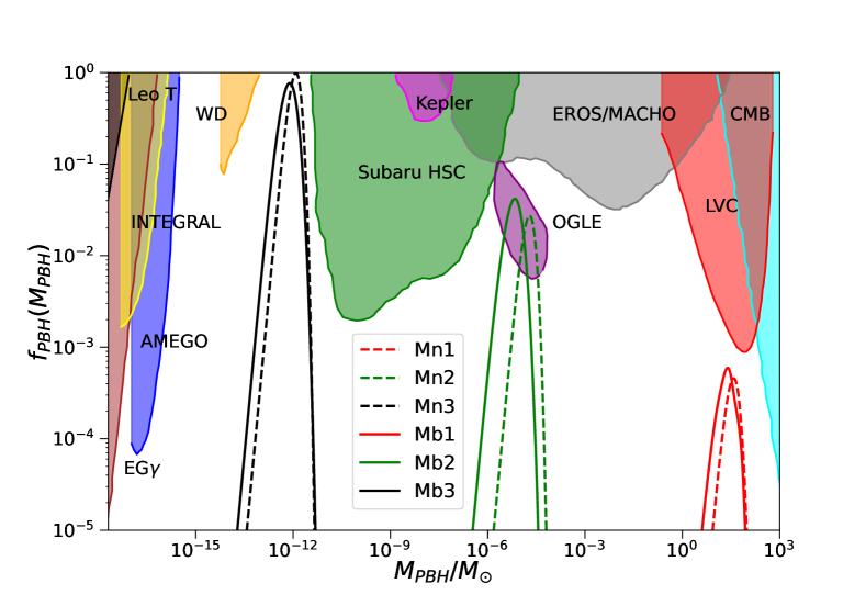
Figure 2: The curves represent PBH mass functions of the models listed in table 1. The most comprehensive constraints on non-evaporated PBHs abundance are displayed in figure 10 of Ref. [154], with the mass of PBHs covering from about $10^{-19}M_{\odot}$ to $10^{22}M_{\odot}$. In this paper, we are interested in the constraints on the PBHs with masses from about $10^{-17}M_{\odot}$ to $10^{3}M_{\odot}$; and the shaded regions show the main observational constraints on the PBH abundance: the cyan region from accretion constraints by CMB [155, 156], the red region from LIGO-Virgo Collaboration measurements [157, 158, 159, 160, 161, 162], the gray region from the EROS/MACHO [163], the green region from microlensing events with Subaru HSC [164], the magenta region from the Kepler satellite [165], the orange region from white dwarf explosion (WD) [166], the blue region from near future MeV telescope AMEGO [167], the yellow region from galactic center 511 keV gamma-ray line (INTEGRAL) [168, 169, 170], the black region from Leo T gas heating [171], the brown region from extragalactic gamma-rays by PBH evaporation (EG$\gamma$) [172]. The purple region are the allowed PBH abundance from the ultrashort-timescale microlensing events in the OGLE data [17].

Model	$\mathcal{P}_{\zeta(\text{peak})}$	$M_{\text{peak}}/M_{\odot}$	$f_{\text{PBH}}$	$f_{c}/\text{Hz}$
Mn1	$5.18\times 10^{-3}$	$38$	$4.71\times 10^{-4}$	$1.83\times 10^{-9}$
Mn2	$4.75\times 10^{-3}$	$1.95\times 10^{-5}$	$2.7\times 10^{-2}$	$2.52\times 10^{-6}$
Mn3	$4.14\times 10^{-3}$	$1.23\times 10^{-12}$	$0.95$	$9.76\times 10^{-3}$
Mb1	$4.59\times 10^{-3}$	$25$	$7.12\times 10^{-4}$	$1.95\times 10^{-9}$
Mb2	$4.11\times 10^{-3}$	$6.93\times 10^{-6}$	$5.39\times 10^{-2}$	$4.01\times 10^{-6}$
Mb3	$3.54\times 10^{-3}$	$7.87\times 10^{-13}$	$0.96$	$1.07\times 10^{-2}$

Table 2: The results for the peak amplitude of primordial scalar power spectrum, the abundance and peak mass of PBHs, and the peak frequency of SIGWs for the inflation models with the chosen parameter sets listed in table 1.

3.3 scalar-induced gravitational waves

In addition to supplying the condition of the formation of PBHs, during radiation domination and after reentering the horizon, the large scalar perturbations can induce the gravitational waves with frequencies ranging from nHz to mHz. The SIGWs with nHz can be detected by PTA and account for the NANOGrav 12.5yrs signal, and those with mHz can be detected by the space-based GW detectors like LISA, Taiji, and TianQin in the future. In the cosmological background and neglecting the anisotropic stress, the perturbed metric in the Newtonian gauge is

$$\begin{split}ds^{2}=-a^{2}(\eta)(1+2\Phi)d\eta^{2}+a^{2}(\eta)\left[(1-2\Phi)\delta_{ij}+\frac{1}{2}h_{ij}\right]dx^{i}dx^{j},\end{split}$$ (3.21)

where $\eta$ is the conformal time, $\Phi$ is the Bardeen potential. The tensor perturbations $h_{ij}$ expressed in the Fourier space are

$$h_{ij}(\bm{x},\eta)=\int\frac{d^{3}ke^{i\bm{k}\cdot\bm{x}}}{(2\pi)^{3/2}}[h_{\bm{k}}(\eta)e_{ij}(\bm{k})+\tilde{h}_{\bm{k}}(\eta)\tilde{e}_{ij}(\bm{k})],$$ (3.22)

where $e_{ij}(\bm{k})$ and $\tilde{e}_{ij}(\bm{k})$ are the plus and cross polarization tensors which can be expressed as

$$e_{ij}(\bm{k})=\frac{1}{\sqrt{2}}\left[e_{i}(\bm{k})e_{j}(\bm{k})-\tilde{e}_{i}(\bm{k})\tilde{e}_{j}(\bm{k})\right],$$ (3.23)

$$\tilde{e}_{ij}(\bm{k})=\frac{1}{\sqrt{2}}\left[e_{i}(\bm{k})\tilde{e}_{j}(\bm{k})+\tilde{e}_{i}(\bm{k})e_{j}(\bm{k})\right],$$ (3.24)

with $\bm{e}\cdot\tilde{\bm{e}}=\bm{e}\cdot\bm{k}=\tilde{\bm{e}}\cdot\bm{k}$.

For either polarization, the tensor perturbations induced from linear scalar perturbations in the Fourier space satisfy [77, 78]

$$h^{\prime\prime}_{\bm{k}}+2\mathcal{H}h^{\prime}_{\bm{k}}+k^{2}h_{\bm{k}}=4S_{\bm{k}},$$ (3.25)

where a prime denotes the derivative with respect to the conformal time, $h^{\prime}_{\bm{k}}=dh_{\bm{k}}/d\eta$, and $\mathcal{H}=a^{\prime}/a$ is the conformal Hubble parameter, $S_{\bm{k}}$ is the second order source from the linear scalar perturbations,

$$\begin{split}S_{\bm{k}}=\int\frac{d^{3}\tilde{k}}{(2\pi)^{3/2}}e_{ij}(\bm{k})\tilde{k}^{i}\tilde{k}^{j}\left[2\Phi_{\tilde{\bm{k}}}\Phi_{\bm{k}-\tilde{\bm{k}}}+\frac{1}{\mathcal{H}^{2}}\left(\Phi^{\prime}_{\tilde{\bm{k}}}+\mathcal{H}\Phi_{\tilde{\bm{k}}}\right)\left(\Phi^{\prime}_{\bm{k}-\tilde{\bm{k}}}+\mathcal{H}\Phi_{\bm{k}-\tilde{\bm{k}}}\right)\right].\end{split}$$ (3.26)

The relation between Bardeen potential $\Phi_{\bm{k}}$ and the primordial curvature perturbation $\zeta_{\bm{k}}$ in Fourier space is

$$\Phi_{\bm{k}}=\frac{3+3w}{5+3w}T(k,\eta)\zeta_{\bm{k}},$$ (3.27)

where $T(k,\eta)$ is the transfer function (3.14). The definition of the power spectrum $\mathcal{P}_{h}(k,\eta)$ for the SIGWs is

$$\langle h_{\bm{k}}(\eta)h_{\tilde{\bm{k}}}(\eta)\rangle=\frac{2\pi^{2}}{k^{3}}\delta^{(3)}(\bm{k}+\tilde{\bm{k}})\mathcal{P}_{h}(k,\eta).$$ (3.28)

The tensor perturbation (3.25) can be solved by the Green function method and the solution is

$$h_{k}(\eta)=\frac{4}{a(\eta)}\int_{\eta_{k}}^{\eta}d\tilde{\eta}g_{k}(\eta,\tilde{\eta})a(\tilde{\eta})S_{k}(\tilde{\eta}),$$ (3.29)

where the corresponding Green function is

$$g_{k}(\eta,\eta^{\prime})=\frac{\sin\left[k(\eta-\eta^{\prime})\right]}{k}.$$ (3.30)

Substituting the result (3.29) into definition (3.28), we obtain [78, 77, 92, 93, 29]

$$\begin{split}\mathcal{P}_{h}(k,\eta)=4\int_{0}^{\infty}dv\int_{|1-v|}^{1+v}du\left[\frac{4v^{2}-(1-u^{2}+v^{2})^{2}}{4uv}\right]^{2}I_{RD}^{2}(u,v,x)\mathcal{P}_{\zeta}(kv)\mathcal{P}_{\zeta}(ku),\end{split}$$ (3.31)

where $u=|\bm{k}-\tilde{\bm{k}}|/k$, $v=\tilde{k}/k$, $x=k\eta$ and the integral kernel $I_{\text{RD}}$ is

$$\begin{split}I_{\text{RD}}(u,v,x)=&\int_{1}^{x}dy\,y\sin(x-y)\{3T(uy)T(vy)\\ &+y[T(vy)uT^{\prime}(uy)+vT^{\prime}(vy)T(uy)]\\ &+y^{2}uvT^{\prime}(uy)T^{\prime}(vy)\}.\end{split}$$ (3.32)

Substituting equation (3.31) into the definition of energy density of SIGWs,

$$\Omega_{\mathrm{GW}}(k,\eta)=\frac{1}{24}\left(\frac{k}{aH}\right)^{2}\overline{\mathcal{P}_{h}(k,\eta)},$$ (3.33)

we get [93, 29]

$$\begin{split}\Omega_{\mathrm{GW}}(k,\eta)=&\frac{1}{6}\left(\frac{k}{aH}\right)^{2}\int_{0}^{\infty}dv\int_{|1-v|}^{1+v}du\left[\frac{4v^{2}-(1-u^{2}+v^{2})^{2}}{4uv}\right]^{2}\\ &\times\overline{I_{\text{RD}}^{2}(u,v,x)}\mathcal{P}_{\zeta}(kv)\mathcal{P}_{\zeta}(ku),\end{split}$$ (3.34)

where $\overline{I_{\text{RD}}^{2}}$ is the oscillation time average of the integral kernel. After formation during the radiation domination, the SIGWs behave like radiation, so the energy density of the SIGWs is in direct proportion to the energy density of the radiation. Using this property, we can obtain the energy density of the SIGWs at present easily and it is

$$\Omega_{\mathrm{GW}}(k,\eta_{0})=c_{g}\Omega_{r,0}\Omega_{\mathrm{GW}}(k,\eta),$$ (3.35)

where $\Omega_{r,0}$ is the energy density of radiation at present, and [130, 128]

$$c_{g}=0.387\left(\frac{g_{*,s}^{4}g_{*}^{-3}}{106.75}\right)^{-1/3}.$$ (3.36)

Substituting the numerical results of the power spectra of the models listed in table 1 into equation (3.34), we obtain the energy density of SIGWs and the numerical results are displayed in figure 3, the corresponding peak frequencies $f_{c}$ are listed in table 2. The SIGWs of models labeled as “1” in table 2 are denoted by the red lines in figure 3 with frequencies around $10^{-9}$ Hz. They are consistent with $2\sigma$ region of the NANOGrav 12.5 yrs signal, which indicates that the NANOGrav 12.5 yrs signal may be SIGWs. The SIGWs of models labeled as “2” in table 2 are denoted by the green lines in figure 3 with frequencies around $10^{-6}$ Hz. The broad peak can be detected by the space-based detectors LISA and Taiji. The SIGWs of models labeled as “3” in table 2 are denoted by the black lines in figure 3 with frequencies around $10^{-3}$ Hz, and can be detected by the LISA, Taiji, TianQin, and DECIGO in the future.

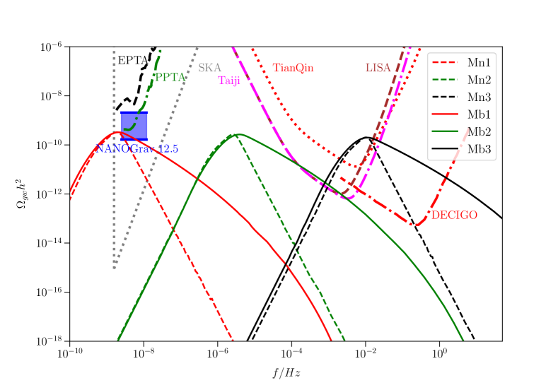
Figure 3: The corresponding scalar-induced secondary gravitational waves from the models listed in table 1. The black dashed curve denotes the EPTA limit [115, 116, 117, 118, 173], the green dot-dashed curve denotes the PPTA limit [174], the gray dotted curve denotes the SKA limit [119], the red dotted curve in the middle denotes the TianQin limit [123], the magenta dot-dashed curve shows the Taiji limit [122], the brown dashed curve shows the LISA limit [121], and the red dot-dashed curve in the right shows the DECIGO limit [124].

4 Conclusion

PBHs and SIGWs can be produced from the inflation models with a transient ultra-slow-roll process, where the equation of motion for the scalar field is $\ddot{\phi}+3H\dot{\phi}\approx 0$. For the scalar-tensor inflation, the ultra-slow-roll condition can be realized by taking $\Omega^{2}/[\omega+3\Omega^{\prime 2}/(2\Omega)]\ll 1$ with $\Omega(\phi)$ coupling to the Ricci scalar and $\omega(\phi)$ to the kinetic term. For the coupling function $\Omega(\phi)$ with quadratic form $\Omega(\phi)=1-2\phi/\phi_{c}+(1+\delta^{2})\left({\phi}/{\phi_{c}}\right)^{2}$, under the condition $\delta^{2}\ll 1$, the ultra-slow condition is satisfied at the point $\phi_{c}$ and the power spectra can be enhanced enough to produce PBHs and generate SIGWs. The parameter $\phi_{c}$ controls the position of the peak in power spectra and also governs the masses of PBHs and the frequencies of SIGWs. The kinetic coupling function is $\omega(\phi)+{3\Omega^{\prime 2}}/{(2\Omega)}=a\Omega^{b}+c\Omega$, determining the shape of the peak in power spectra.

In this paper, we produce three kinds of PBHs: the PBHs with stellar masses, those with planetary masses, and those with masses around $10^{-12}M_{\odot}$. The cases with a narrow peak and a broad peak are both given for each kind. The first kind PBHs have the peak masses $M_{\text{peak}}=38M_{\odot}$ (narrow peak) and $M_{\text{peak}}=25M_{\odot}$ (broad peak), and may be the sources of the GWs in the LIGO/Virgo events. The corresponding SIGWs have the peak frequencies around $10^{-9}$ Hz and can explain the NANOGrav 12.5yrs signal. The second kind PBHs have the peak masses $M_{\text{peak}}=1.95\times 10^{-5}M_{\odot}$ (narrow peak) and $M_{\text{peak}}=6.93\times 10^{-6}M_{\odot}$ (broad peak), can explain the ultrashort-timescale microlensing events in the OGLE data. The corresponding SIGWs have the peak frequencies around $10^{-6}$ Hz, and the broad peak case can be detected by the space-based detectors LISA and Taiji. The third kind PBHs have peak masses $M_{\text{peak}}=1.23\times 10^{-12}M_{\odot}$ (narrow peak) with the PBHs abundance $f_{\text{PBH}}=0.95$, and $M_{\text{peak}}=7.87\times 10^{-13}M_{\odot}$ (broad peak) with the PBHs abundance $f_{\text{PBH}}=0.96$, they can account for almost all of the dark matter. The corresponding SIGWs have the peak frequencies around $10^{-3}$ Hz and can be detected by the space-based detectors LISA, Taiji, TianQin, and DECIGO. The scalar tilt and tensor-to-scalar ratio of these models are about $n_{s}\approx 0.965,\quad r\approx 0.004$ with the $e$-folds $N\approx 60$, which are consistent with the Planck 2018 observational data.

In conclusion, the scalar-tensor inflation with the quadratic form coupling function $\Omega(\phi)=1-2\phi/\phi_{c}+(1+\delta^{2})\left({\phi}/{\phi_{c}}\right)^{2}$ can successfully enhance the power spectra, produce the PBHs, and generate the SIGWs. The masses of the PBHs and the frequencies of the SIGWs can be adjusted by the parameter $\phi_{c}$, and the shape of the peak can be adjusted by the coupling function $\omega(\phi)$.

References

- [1] B.J. Carr and S.W. Hawking, Black holes in the early Universe, Mon. Not. Roy. Astron. Soc. 168 (1974) 399.
- [2] S. Hawking, Gravitationally collapsed objects of very low mass, Mon. Not. Roy. Astron. Soc. 152 (1971) 75.
- [3] S. Bird, I. Cholis, J.B. Muñoz, Y. Ali-Haïmoud, M. Kamionkowski, E.D. Kovetz et al., Did LIGO detect dark matter?, Phys. Rev. Lett. 116 (2016) 201301 [1603.00464].
- [4] M. Sasaki, T. Suyama, T. Tanaka and S. Yokoyama, Primordial Black Hole Scenario for the Gravitational-Wave Event GW150914, Phys. Rev. Lett. 117 (2016) 061101 [1603.08338].
- [5] LIGO Scientific, Virgo collaboration, Observation of Gravitational Waves from a Binary Black Hole Merger, Phys. Rev. Lett. 116 (2016) 061102 [1602.03837].
- [6] LIGO Scientific, Virgo collaboration, GW151226: Observation of Gravitational Waves from a 22-Solar-Mass Binary Black Hole Coalescence, Phys. Rev. Lett. 116 (2016) 241103 [1606.04855].
- [7] LIGO Scientific, VIRGO collaboration, GW170104: Observation of a 50-Solar-Mass Binary Black Hole Coalescence at Redshift 0.2, Phys. Rev. Lett. 118 (2017) 221101 [1706.01812].
- [8] LIGO Scientific, Virgo collaboration, GW170814: A Three-Detector Observation of Gravitational Waves from a Binary Black Hole Coalescence, Phys. Rev. Lett. 119 (2017) 141101 [1709.09660].
- [9] LIGO Scientific, Virgo collaboration, GW170817: Observation of Gravitational Waves from a Binary Neutron Star Inspiral, Phys. Rev. Lett. 119 (2017) 161101 [1710.05832].
- [10] LIGO Scientific, Virgo collaboration, GW170608: Observation of a 19-solar-mass Binary Black Hole Coalescence, Astrophys. J. Lett. 851 (2017) L35 [1711.05578].
- [11] LIGO Scientific, Virgo collaboration, GWTC-1: A Gravitational-Wave Transient Catalog of Compact Binary Mergers Observed by LIGO and Virgo during the First and Second Observing Runs, Phys. Rev. X 9 (2019) 031040 [1811.12907].
- [12] LIGO Scientific, Virgo collaboration, GW190425: Observation of a Compact Binary Coalescence with Total Mass , Astrophys. J. Lett. 892 (2020) L3 [2001.01761].
- [13] LIGO Scientific, Virgo collaboration, GW190412: Observation of a Binary-Black-Hole Coalescence with Asymmetric Masses, Phys. Rev. D 102 (2020) 043015 [2004.08342].
- [14] LIGO Scientific, Virgo collaboration, GW190814: Gravitational Waves from the Coalescence of a 23 Solar Mass Black Hole with a 2.6 Solar Mass Compact Object, Astrophys. J. Lett. 896 (2020) L44 [2006.12611].
- [15] LIGO Scientific, Virgo collaboration, GW190521: A Binary Black Hole Merger with a Total Mass of , Phys. Rev. Lett. 125 (2020) 101102 [2009.01075].
- [16] LIGO Scientific, Virgo collaboration, GWTC-2: Compact Binary Coalescences Observed by LIGO and Virgo During the First Half of the Third Observing Run, Phys. Rev. X 11 (2021) 021053 [2010.14527].
- [17] H. Niikura, M. Takada, S. Yokoyama, T. Sumi and S. Masaki, Constraints on Earth-mass primordial black holes from OGLE 5-year microlensing events, Phys. Rev. D 99 (2019) 083503 [1901.07120].
- [18] J. Scholtz and J. Unwin, What if Planet 9 is a Primordial Black Hole?, Phys. Rev. Lett. 125 (2020) 051103 [1909.11090].
- [19] P. Ivanov, P. Naselsky and I. Novikov, Inflation and primordial black holes as dark matter, Phys. Rev. D 50 (1994) 7173.
- [20] P.H. Frampton, M. Kawasaki, F. Takahashi and T.T. Yanagida, Primordial Black Holes as All Dark Matter, JCAP 04 (2010) 023 [1001.2308].
- [21] K.M. Belotsky, A.D. Dmitriev, E.A. Esipova, V.A. Gani, A.V. Grobov, M.Y. Khlopov et al., Signatures of primordial black hole dark matter, Mod. Phys. Lett. A 29 (2014) 1440005 [1410.0203].
- [22] M.Y. Khlopov, S.G. Rubin and A.S. Sakharov, Primordial structure of massive black hole clusters, Astropart. Phys. 23 (2005) 265 [astro-ph/0401532].
- [23] B. Carr, F. Kuhnel and M. Sandstad, Primordial Black Holes as Dark Matter, Phys. Rev. D 94 (2016) 083504 [1607.06077].
- [24] K. Inomata, M. Kawasaki, K. Mukaida, Y. Tada and T.T. Yanagida, Inflationary Primordial Black Holes as All Dark Matter, Phys. Rev. D 96 (2017) 043504 [1701.02544].
- [25] J. García-Bellido, Massive Primordial Black Holes as Dark Matter and their detection with Gravitational Waves, J. Phys. Conf. Ser. 840 (2017) 012032 [1702.08275].
- [26] E.D. Kovetz, Probing Primordial-Black-Hole Dark Matter with Gravitational Waves, Phys. Rev. Lett. 119 (2017) 131301 [1705.09182].
- [27] B. Carr and F. Kuhnel, Primordial Black Holes as Dark Matter: Recent Developments, Ann. Rev. Nucl. Part. Sci. 70 (2020) 355 [2006.02838].
- [28] H. Di and Y. Gong, Primordial black holes and second order gravitational waves from ultra-slow-roll inflation, JCAP 07 (2018) 007 [1707.09578].
- [29] Y. Lu, Y. Gong, Z. Yi and F. Zhang, Constraints on primordial curvature perturbations from primordial black hole dark matter and secondary gravitational waves, JCAP 12 (2019) 031 [1907.11896].
- [30] G. Sato-Polito, E.D. Kovetz and M. Kamionkowski, Constraints on the primordial curvature power spectrum from primordial black holes, Phys. Rev. D 100 (2019) 063521 [1904.10971].
- [31] Planck collaboration, Planck 2018 results. X. Constraints on inflation, Astron. Astrophys. 641 (2020) A10 [1807.06211].
- [32] J. Martin, H. Motohashi and T. Suyama, Ultra Slow-Roll Inflation and the non-Gaussianity Consistency Relation, Phys. Rev. D 87 (2013) 023514 [1211.0083].
- [33] H. Motohashi, A.A. Starobinsky and J. Yokoyama, Inflation with a constant rate of roll, JCAP 09 (2015) 018 [1411.5021].
- [34] Z. Yi and Y. Gong, On the constant-roll inflation, JCAP 03 (2018) 052 [1712.07478].
- [35] J. Garcia-Bellido and E. Ruiz Morales, Primordial black holes from single field models of inflation, Phys. Dark Univ. 18 (2017) 47 [1702.03901].
- [36] C. Germani and T. Prokopec, On primordial black holes from an inflection point, Phys. Dark Univ. 18 (2017) 6 [1706.04226].
- [37] H. Motohashi and W. Hu, Primordial Black Holes and Slow-Roll Violation, Phys. Rev. D 96 (2017) 063503 [1706.06784].
- [38] J.M. Ezquiaga, J. Garcia-Bellido and E. Ruiz Morales, Primordial Black Hole production in Critical Higgs Inflation, Phys. Lett. B 776 (2018) 345 [1705.04861].
- [39] G. Ballesteros, J. Beltran Jimenez and M. Pieroni, Black hole formation from a general quadratic action for inflationary primordial fluctuations, JCAP 06 (2019) 016 [1811.03065].
- [40] I. Dalianis, A. Kehagias and G. Tringas, Primordial black holes from -attractors, JCAP 01 (2019) 037 [1805.09483].
- [41] F. Bezrukov, M. Pauly and J. Rubio, On the robustness of the primordial power spectrum in renormalized Higgs inflation, JCAP 02 (2018) 040 [1706.05007].
- [42] K. Kannike, L. Marzola, M. Raidal and H. Veermäe, Single Field Double Inflation and Primordial Black Holes, JCAP 09 (2017) 020 [1705.06225].
- [43] M. Sasaki, T. Suyama, T. Tanaka and S. Yokoyama, Primordial black holes—perspectives in gravitational wave astronomy, Class. Quant. Grav. 35 (2018) 063001 [1801.05235].
- [44] S. Passaglia, W. Hu and H. Motohashi, Primordial black holes and local non-Gaussianity in canonical inflation, Phys. Rev. D 99 (2019) 043536 [1812.08243].
- [45] J. Lin, Q. Gao, Y. Gong, Y. Lu, C. Zhang and F. Zhang, Primordial black holes and secondary gravitational waves from and inflation, Phys. Rev. D 101 (2020) 103515 [2001.05909].
- [46] J. Lin, S. Gao, Y. Gong, Y. Lu, Z. Wang and F. Zhang, Primordial black holes and scalar induced gravitational waves from Higgs inflation with noncanonical kinetic term, Phys. Rev. D 107 (2023) 043517 [2111.01362].
- [47] Q. Gao, Y. Gong and Z. Yi, Primordial black holes and secondary gravitational waves from natural inflation, Nucl. Phys. B 969 (2021) 115480 [2012.03856].
- [48] Q. Gao, Primordial black holes and secondary gravitational waves from chaotic inflation, Sci. China Phys. Mech. Astron. 64 (2021) 280411 [2102.07369].
- [49] Z. Yi, Y. Gong, B. Wang and Z.-h. Zhu, Primordial black holes and secondary gravitational waves from the Higgs field, Phys. Rev. D 103 (2021) 063535 [2007.09957].
- [50] Z. Yi, Q. Gao, Y. Gong and Z.-h. Zhu, Primordial black holes and scalar-induced secondary gravitational waves from inflationary models with a noncanonical kinetic term, Phys. Rev. D 103 (2021) 063534 [2011.10606].
- [51] Z. Yi and Z.-H. Zhu, NANOGrav signal and LIGO-Virgo primordial black holes from the Higgs field, JCAP 05 (2022) 046 [2105.01943].
- [52] F. Zhang, Y. Gong, J. Lin, Y. Lu and Z. Yi, Primordial non-Gaussianity from G-inflation, JCAP 04 (2021) 045 [2012.06960].
- [53] S. Pi, Y.-l. Zhang, Q.-G. Huang and M. Sasaki, Scalaron from -gravity as a heavy field, JCAP 05 (2018) 042 [1712.09896].
- [54] A.Y. Kamenshchik, A. Tronconi, T. Vardanyan and G. Venturi, Non-Canonical Inflation and Primordial Black Holes Production, Phys. Lett. B 791 (2019) 201 [1812.02547].
- [55] C. Fu, P. Wu and H. Yu, Primordial Black Holes from Inflation with Nonminimal Derivative Coupling, Phys. Rev. D 100 (2019) 063532 [1907.05042].
- [56] C. Fu, P. Wu and H. Yu, Scalar induced gravitational waves in inflation with gravitationally enhanced friction, Phys. Rev. D 101 (2020) 023529 [1912.05927].
- [57] I. Dalianis, S. Karydas and E. Papantonopoulos, Generalized Non-Minimal Derivative Coupling: Application to Inflation and Primordial Black Hole Production, JCAP 06 (2020) 040 [1910.00622].
- [58] A. Gundhi and C.F. Steinwachs, Scalaron–Higgs inflation reloaded: Higgs-dependent scalaron mass and primordial black hole dark matter, Eur. Phys. J. C 81 (2021) 460 [2011.09485].
- [59] D.Y. Cheong, S.M. Lee and S.C. Park, Primordial black holes in Higgs- inflation as the whole of dark matter, JCAP 01 (2021) 032 [1912.12032].
- [60] F. Zhang, Primordial black holes and scalar induced gravitational waves from the E model with a Gauss-Bonnet term, Phys. Rev. D 105 (2022) 063539 [2112.10516].
- [61] S. Kawai and J. Kim, Primordial black holes from Gauss-Bonnet-corrected single field inflation, Phys. Rev. D 104 (2021) 083545 [2108.01340].
- [62] R.-G. Cai, C. Chen and C. Fu, Primordial black holes and stochastic gravitational wave background from inflation with a noncanonical spectator field, Phys. Rev. D 104 (2021) 083537 [2108.03422].
- [63] P. Chen, S. Koh and G. Tumurtushaa, Primordial black holes and induced gravitational waves from inflation in the Horndeski theory of gravity, 2107.08638.
- [64] R. Zheng, J. Shi and T. Qiu, On primordial black holes and secondary gravitational waves generated from inflation with solo/multi-bumpy potential *, Chin. Phys. C 46 (2022) 045103 [2106.04303].
- [65] A. Karam, N. Koivunen, E. Tomberg, V. Vaskonen and H. Veermäe, Anatomy of single-field inflationary models for primordial black holes, 2205.13540.
- [66] A. Ashoorioon, R. Casadio, M. Cicoli, G. Geshnizjani and H.J. Kim, Extended Effective Field Theory of Inflation, JHEP 02 (2018) 172 [1802.03040].
- [67] A. Ashoorioon, A. Rostami and J.T. Firouzjaee, EFT compatible PBHs: effective spawning of the seeds for primordial black holes during inflation, JHEP 07 (2021) 087 [1912.13326].
- [68] J. Garcia-Bellido, A.D. Linde and D. Wands, Density perturbations and black hole formation in hybrid inflation, Phys. Rev. D 54 (1996) 6040 [astro-ph/9605094].
- [69] S. Clesse and J. García-Bellido, Massive Primordial Black Holes from Hybrid Inflation as Dark Matter and the seeds of Galaxies, Phys. Rev. D 92 (2015) 023524 [1501.07565].
- [70] G.A. Palma, S. Sypsas and C. Zenteno, Seeding primordial black holes in multifield inflation, Phys. Rev. Lett. 125 (2020) 121301 [2004.06106].
- [71] M. Braglia, D.K. Hazra, F. Finelli, G.F. Smoot, L. Sriramkumar and A.A. Starobinsky, Generating PBHs and small-scale GWs in two-field models of inflation, JCAP 08 (2020) 001 [2005.02895].
- [72] J. Fumagalli, S. Renaux-Petel and L.T. Witkowski, Oscillations in the stochastic gravitational wave background from sharp features and particle production during inflation, JCAP 08 (2021) 030 [2012.02761].
- [73] D.Y. Cheong, K. Kohri and S.C. Park, The inflaton that could: primordial black holes and second order gravitational waves from tachyonic instability induced in Higgs-R 2 inflation, JCAP 10 (2022) 015 [2205.14813].
- [74] J. Kristiano and J. Yokoyama, Ruling Out Primordial Black Hole Formation From Single-Field Inflation, 2211.03395.
- [75] S. Matarrese, S. Mollerach and M. Bruni, Second order perturbations of the Einstein-de Sitter universe, Phys. Rev. D 58 (1998) 043504 [astro-ph/9707278].
- [76] S. Mollerach, D. Harari and S. Matarrese, CMB polarization from secondary vector and tensor modes, Phys. Rev. D 69 (2004) 063002 [astro-ph/0310711].
- [77] K.N. Ananda, C. Clarkson and D. Wands, The Cosmological gravitational wave background from primordial density perturbations, Phys. Rev. D 75 (2007) 123518 [gr-qc/0612013].
- [78] D. Baumann, P.J. Steinhardt, K. Takahashi and K. Ichiki, Gravitational Wave Spectrum Induced by Primordial Scalar Perturbations, Phys. Rev. D 76 (2007) 084019 [hep-th/0703290].
- [79] J. Garcia-Bellido, M. Peloso and C. Unal, Gravitational Wave signatures of inflationary models from Primordial Black Hole Dark Matter, JCAP 09 (2017) 013 [1707.02441].
- [80] R. Saito and J. Yokoyama, Gravitational wave background as a probe of the primordial black hole abundance, Phys. Rev. Lett. 102 (2009) 161101 [0812.4339].
- [81] R. Saito and J. Yokoyama, Gravitational-Wave Constraints on the Abundance of Primordial Black Holes, Prog. Theor. Phys. 123 (2010) 867 [0912.5317].
- [82] E. Bugaev and P. Klimai, Induced gravitational wave background and primordial black holes, Phys. Rev. D 81 (2010) 023517 [0908.0664].
- [83] E. Bugaev and P. Klimai, Constraints on the induced gravitational wave background from primordial black holes, Phys. Rev. D 83 (2011) 083521 [1012.4697].
- [84] L. Alabidi, K. Kohri, M. Sasaki and Y. Sendouda, Observable Spectra of Induced Gravitational Waves from Inflation, JCAP 09 (2012) 017 [1203.4663].
- [85] N. Orlofsky, A. Pierce and J.D. Wells, Inflationary theory and pulsar timing investigations of primordial black holes and gravitational waves, Phys. Rev. D 95 (2017) 063518 [1612.05279].
- [86] T. Nakama, J. Silk and M. Kamionkowski, Stochastic gravitational waves associated with the formation of primordial black holes, Phys. Rev. D 95 (2017) 043511 [1612.06264].
- [87] K. Inomata, M. Kawasaki, K. Mukaida, Y. Tada and T.T. Yanagida, Inflationary primordial black holes for the LIGO gravitational wave events and pulsar timing array experiments, Phys. Rev. D 95 (2017) 123510 [1611.06130].
- [88] S.-L. Cheng, W. Lee and K.-W. Ng, Primordial black holes and associated gravitational waves in axion monodromy inflation, JCAP 07 (2018) 001 [1801.09050].
- [89] R.-g. Cai, S. Pi and M. Sasaki, Gravitational Waves Induced by non-Gaussian Scalar Perturbations, Phys. Rev. Lett. 122 (2019) 201101 [1810.11000].
- [90] N. Bartolo, V. De Luca, G. Franciolini, M. Peloso, D. Racco and A. Riotto, Testing primordial black holes as dark matter with LISA, Phys. Rev. D 99 (2019) 103521 [1810.12224].
- [91] N. Bartolo, V. De Luca, G. Franciolini, A. Lewis, M. Peloso and A. Riotto, Primordial Black Hole Dark Matter: LISA Serendipity, Phys. Rev. Lett. 122 (2019) 211301 [1810.12218].
- [92] K. Kohri and T. Terada, Semianalytic calculation of gravitational wave spectrum nonlinearly induced from primordial curvature perturbations, Phys. Rev. D 97 (2018) 123532 [1804.08577].
- [93] J.R. Espinosa, D. Racco and A. Riotto, A Cosmological Signature of the SM Higgs Instability: Gravitational Waves, JCAP 09 (2018) 012 [1804.07732].
- [94] R.-G. Cai, S. Pi, S.-J. Wang and X.-Y. Yang, Resonant multiple peaks in the induced gravitational waves, JCAP 05 (2019) 013 [1901.10152].
- [95] R.-G. Cai, S. Pi, S.-J. Wang and X.-Y. Yang, Pulsar Timing Array Constraints on the Induced Gravitational Waves, JCAP 10 (2019) 059 [1907.06372].
- [96] R.-G. Cai, Z.-K. Guo, J. Liu, L. Liu and X.-Y. Yang, Primordial black holes and gravitational waves from parametric amplification of curvature perturbations, JCAP 06 (2020) 013 [1912.10437].
- [97] R.-G. Cai, Y.-C. Ding, X.-Y. Yang and Y.-F. Zhou, Constraints on a mixed model of dark matter particles and primordial black holes from the galactic 511 keV line, JCAP 03 (2021) 057 [2007.11804].
- [98] G. Domènech, Induced gravitational waves in a general cosmological background, Int. J. Mod. Phys. D 29 (2020) 2050028 [1912.05583].
- [99] G. Domènech, S. Pi and M. Sasaki, Induced gravitational waves as a probe of thermal history of the universe, JCAP 08 (2020) 017 [2005.12314].
- [100] J. Fumagalli, S. Renaux-Petel, J.W. Ronayne and L.T. Witkowski, Turning in the landscape: a new mechanism for generating Primordial Black Holes, 2004.08369.
- [101] A. Ashoorioon, A. Rostami and J.T. Firouzjaee, Examining the end of inflation with primordial black holes mass distribution and gravitational waves, Phys. Rev. D 103 (2021) 123512 [2012.02817].
- [102] A. Ashoorioon, K. Rezazadeh and A. Rostami, NANOGrav signal from the end of inflation and the LIGO mass and heavier primordial black holes, Phys. Lett. B 835 (2022) 137542 [2202.01131].
- [103] S. Pi and M. Sasaki, Gravitational Waves Induced by Scalar Perturbations with a Lognormal Peak, JCAP 09 (2020) 037 [2005.12306].
- [104] C. Yuan, Z.-C. Chen and Q.-G. Huang, Scalar induced gravitational waves in different gauges, Phys. Rev. D 101 (2020) 063018 [1912.00885].
- [105] C. Yuan, Z.-C. Chen and Q.-G. Huang, Log-dependent slope of scalar induced gravitational waves in the infrared regions, Phys. Rev. D 101 (2020) 043019 [1910.09099].
- [106] C. Yuan, Z.-C. Chen and Q.-G. Huang, Probing primordial–black-hole dark matter with scalar induced gravitational waves, Phys. Rev. D 100 (2019) 081301 [1906.11549].
- [107] T. Papanikolaou, V. Vennin and D. Langlois, Gravitational waves from a universe filled with primordial black holes, JCAP 03 (2021) 053 [2010.11573].
- [108] T. Papanikolaou, C. Tzerefos, S. Basilakos and E.N. Saridakis, Scalar induced gravitational waves from primordial black hole Poisson fluctuations in f(R) gravity, JCAP 10 (2022) 013 [2112.15059].
- [109] T. Papanikolaou, C. Tzerefos, S. Basilakos and E.N. Saridakis, No constraints for f(T) gravity from gravitational waves induced from primordial black hole fluctuations, Eur. Phys. J. C 83 (2023) 31 [2205.06094].
- [110] G. Domènech, Scalar Induced Gravitational Waves Review, Universe 7 (2021) 398 [2109.01398].
- [111] V. Atal and G. Domènech, Probing non-Gaussianities with the high frequency tail of induced gravitational waves, JCAP 06 (2021) 001 [2103.01056].
- [112] S. Balaji, G. Domenech and J. Silk, Induced gravitational waves from slow-roll inflation after an enhancing phase, JCAP 09 (2022) 016 [2205.01696].
- [113] J.-X. Feng, F. Zhang and X. Gao, Scalar induced gravitational waves from Chern-Simons gravity during inflation era, 2302.00950.
- [114] F. Zhang, J.-X. Feng and X. Gao, Circularly polarized scalar induced gravitational waves from the Chern-Simons modified gravity, JCAP 10 (2022) 054 [2205.12045].
- [115] R.D. Ferdman et al., The European Pulsar Timing Array: current efforts and a LEAP toward the future, Class. Quant. Grav. 27 (2010) 084014 [1003.3405].
- [116] G. Hobbs et al., The international pulsar timing array project: using pulsars as a gravitational wave detector, Class. Quant. Grav. 27 (2010) 084013 [0911.5206].
- [117] M.A. McLaughlin, The North American Nanohertz Observatory for Gravitational Waves, Class. Quant. Grav. 30 (2013) 224008 [1310.0758].
- [118] G. Hobbs, The Parkes Pulsar Timing Array, Class. Quant. Grav. 30 (2013) 224007 [1307.2629].
- [119] C.J. Moore, R.H. Cole and C.P.L. Berry, Gravitational-wave sensitivity curves, Class. Quant. Grav. 32 (2015) 015014 [1408.0740].
- [120] K. Danzmann, LISA: An ESA cornerstone mission for a gravitational wave observatory, Class. Quant. Grav. 14 (1997) 1399.
- [121] LISA collaboration, Laser Interferometer Space Antenna, 1702.00786.
- [122] W.-R. Hu and Y.-L. Wu, The Taiji Program in Space for gravitational wave physics and the nature of gravity, Natl. Sci. Rev. 4 (2017) 685.
- [123] TianQin collaboration, TianQin: a space-borne gravitational wave detector, Class. Quant. Grav. 33 (2016) 035010 [1512.02076].
- [124] S. Kawamura et al., The Japanese space gravitational wave antenna: DECIGO, Class. Quant. Grav. 28 (2011) 094011.
- [125] NANOGrav collaboration, The NANOGrav 12.5 yr Data Set: Search for an Isotropic Stochastic Gravitational-wave Background, Astrophys. J. Lett. 905 (2020) L34 [2009.04496].
- [126] B. Goncharov et al., On the Evidence for a Common-spectrum Process in the Search for the Nanohertz Gravitational-wave Background with the Parkes Pulsar Timing Array, Astrophys. J. Lett. 917 (2021) L19 [2107.12112].
- [127] J. Antoniadis et al., The International Pulsar Timing Array second data release: Search for an isotropic gravitational wave background, Mon. Not. Roy. Astron. Soc. 510 (2022) 4873 [2201.03980].
- [128] V. De Luca, G. Franciolini and A. Riotto, NANOGrav Data Hints at Primordial Black Holes as Dark Matter, Phys. Rev. Lett. 126 (2021) 041303 [2009.08268].
- [129] K. Inomata, M. Kawasaki, K. Mukaida and T.T. Yanagida, NANOGrav Results and LIGO-Virgo Primordial Black Holes in Axionlike Curvaton Models, Phys. Rev. Lett. 126 (2021) 131301 [2011.01270].
- [130] V. Vaskonen and H. Veermäe, Did NANOGrav see a signal from primordial black hole formation?, Phys. Rev. Lett. 126 (2021) 051303 [2009.07832].
- [131] G. Domènech and S. Pi, NANOGrav hints on planet-mass primordial black holes, Sci. China Phys. Mech. Astron. 65 (2022) 230411 [2010.03976].
- [132] Z. Yi and Q. Fei, Constraints on primordial curvature spectrum from primordial black holes and scalar-induced gravitational waves, Eur. Phys. J. C 83 (2023) 82 [2210.03641].
- [133] D.F. Torres, Slow roll inflation in nonminimally coupled theories: Hyperextended gravity approach, Phys. Lett. A 225 (1997) 13 [gr-qc/9610021].
- [134] Planck collaboration, Planck 2018 results. X. Constraints on inflation, Astron. Astrophys. 641 (2020) A10 [1807.06211].
- [135] F.L. Bezrukov and M. Shaposhnikov, The Standard Model Higgs boson as the inflaton, Phys. Lett. B 659 (2008) 703 [0710.3755].
- [136] J.-c. Hwang, Quantum fluctuations of cosmological perturbations in generalized gravity, Class. Quant. Grav. 14 (1997) 3327 [gr-qc/9607059].
- [137] BICEP2, Keck Array collaboration, BICEP2 / Keck Array x: Constraints on Primordial Gravitational Waves using Planck, WMAP, and New BICEP2/Keck Observations through the 2015 Season, Phys. Rev. Lett. 121 (2018) 221301 [1810.05216].
- [138] K. Inomata and T. Nakama, Gravitational waves induced by scalar perturbations as probes of the small-scale primordial spectrum, Phys. Rev. D 99 (2019) 043511 [1812.00674].
- [139] K. Inomata, M. Kawasaki and Y. Tada, Revisiting constraints on small scale perturbations from big-bang nucleosynthesis, Phys. Rev. D 94 (2016) 043527 [1605.04646].
- [140] D.J. Fixsen, E.S. Cheng, J.M. Gales, J.C. Mather, R.A. Shafer and E.L. Wright, The Cosmic Microwave Background spectrum from the full COBE FIRAS data set, Astrophys. J. 473 (1996) 576 [astro-ph/9605054].
- [141] J.M. Bardeen, J.R. Bond, N. Kaiser and A.S. Szalay, The Statistics of Peaks of Gaussian Random Fields, Astrophys. J. 304 (1986) 15.
- [142] A.M. Green, A.R. Liddle, K.A. Malik and M. Sasaki, A New calculation of the mass fraction of primordial black holes, Phys. Rev. D 70 (2004) 041502 [astro-ph/0403181].
- [143] S. Young, C.T. Byrnes and M. Sasaki, Calculating the mass fraction of primordial black holes, JCAP 07 (2014) 045 [1405.7023].
- [144] C. Germani and I. Musco, Abundance of Primordial Black Holes Depends on the Shape of the Inflationary Power Spectrum, Phys. Rev. Lett. 122 (2019) 141302 [1805.04087].
- [145] S. Young and M. Musso, Application of peaks theory to the abundance of primordial black holes, JCAP 11 (2020) 022 [2001.06469].
- [146] A.D. Gow, C.T. Byrnes, P.S. Cole and S. Young, The power spectrum on small scales: Robust constraints and comparing PBH methodologies, JCAP 02 (2021) 002 [2008.03289].
- [147] K. Ando, K. Inomata and M. Kawasaki, Primordial black holes and uncertainties in the choice of the window function, Phys. Rev. D 97 (2018) 103528 [1802.06393].
- [148] I. Musco, Threshold for primordial black holes: Dependence on the shape of the cosmological perturbations, Phys. Rev. D 100 (2019) 123524 [1809.02127].
- [149] S. Young, The primordial black hole formation criterion re-examined: Parametrisation, timing and the choice of window function, Int. J. Mod. Phys. D 29 (2019) 2030002 [1905.01230].
- [150] M.W. Choptuik, Universality and scaling in gravitational collapse of a massless scalar field, Phys. Rev. Lett. 70 (1993) 9.
- [151] C.R. Evans and J.S. Coleman, Observation of critical phenomena and selfsimilarity in the gravitational collapse of radiation fluid, Phys. Rev. Lett. 72 (1994) 1782 [gr-qc/9402041].
- [152] J.C. Niemeyer and K. Jedamzik, Near-critical gravitational collapse and the initial mass function of primordial black holes, Phys. Rev. Lett. 80 (1998) 5481 [astro-ph/9709072].
- [153] C.T. Byrnes, M. Hindmarsh, S. Young and M.R.S. Hawkins, Primordial black holes with an accurate QCD equation of state, JCAP 08 (2018) 041 [1801.06138].
- [154] B. Carr, K. Kohri, Y. Sendouda and J. Yokoyama, Constraints on primordial black holes, Rept. Prog. Phys. 84 (2021) 116902 [2002.12778].
- [155] Y. Ali-Haïmoud and M. Kamionkowski, Cosmic microwave background limits on accreting primordial black holes, Phys. Rev. D 95 (2017) 043534 [1612.05644].
- [156] V. Poulin, P.D. Serpico, F. Calore, S. Clesse and K. Kohri, CMB bounds on disk-accreting massive primordial black holes, Phys. Rev. D 96 (2017) 083524 [1707.04206].
- [157] Y. Ali-Haïmoud, E.D. Kovetz and M. Kamionkowski, Merger rate of primordial black-hole binaries, Phys. Rev. D 96 (2017) 123523 [1709.06576].
- [158] M. Raidal, C. Spethmann, V. Vaskonen and H. Veermäe, Formation and Evolution of Primordial Black Hole Binaries in the Early Universe, JCAP 02 (2019) 018 [1812.01930].
- [159] V. Vaskonen and H. Veermäe, Lower bound on the primordial black hole merger rate, Phys. Rev. D 101 (2020) 043015 [1908.09752].
- [160] V. De Luca, G. Franciolini, P. Pani and A. Riotto, Primordial Black Holes Confront LIGO/Virgo data: Current situation, JCAP 06 (2020) 044 [2005.05641].
- [161] K.W.K. Wong, G. Franciolini, V. De Luca, V. Baibhav, E. Berti, P. Pani et al., Constraining the primordial black hole scenario with Bayesian inference and machine learning: the GWTC-2 gravitational wave catalog, Phys. Rev. D 103 (2021) 023026 [2011.01865].
- [162] G. Hütsi, M. Raidal, V. Vaskonen and H. Veermäe, Two populations of LIGO-Virgo black holes, JCAP 03 (2021) 068 [2012.02786].
- [163] EROS-2 collaboration, Limits on the Macho Content of the Galactic Halo from the EROS-2 Survey of the Magellanic Clouds, Astron. Astrophys. 469 (2007) 387 [astro-ph/0607207].
- [164] H. Niikura et al., Microlensing constraints on primordial black holes with Subaru/HSC Andromeda observations, Nature Astron. 3 (2019) 524 [1701.02151].
- [165] K. Griest, A.M. Cieplak and M.J. Lehner, New Limits on Primordial Black Hole Dark Matter from an Analysis of Kepler Source Microlensing Data, Phys. Rev. Lett. 111 (2013) 181302.
- [166] P.W. Graham, S. Rajendran and J. Varela, Dark Matter Triggers of Supernovae, Phys. Rev. D 92 (2015) 063007 [1505.04444].
- [167] A. Ray, R. Laha, J.B. Muñoz and R. Caputo, Near future MeV telescopes can discover asteroid-mass primordial black hole dark matter, Phys. Rev. D 104 (2021) 023516 [2102.06714].
- [168] R. Laha, Primordial Black Holes as a Dark Matter Candidate Are Severely Constrained by the Galactic Center 511 keV -Ray Line, Phys. Rev. Lett. 123 (2019) 251101 [1906.09994].
- [169] B. Dasgupta, R. Laha and A. Ray, Neutrino and positron constraints on spinning primordial black hole dark matter, Phys. Rev. Lett. 125 (2020) 101101 [1912.01014].
- [170] R. Laha, J.B. Muñoz and T.R. Slatyer, INTEGRAL constraints on primordial black holes and particle dark matter, Phys. Rev. D 101 (2020) 123514 [2004.00627].
- [171] R. Laha, P. Lu and V. Takhistov, Gas heating from spinning and non-spinning evaporating primordial black holes, Phys. Lett. B 820 (2021) 136459 [2009.11837].
- [172] B.J. Carr, K. Kohri, Y. Sendouda and J. Yokoyama, New cosmological constraints on primordial black holes, Phys. Rev. D 81 (2010) 104019 [0912.5297].
- [173] L. Lentati et al., European Pulsar Timing Array Limits On An Isotropic Stochastic Gravitational-Wave Background, Mon. Not. Roy. Astron. Soc. 453 (2015) 2576 [1504.03692].
- [174] R.M. Shannon et al., Gravitational waves from binary supermassive black holes missing in pulsar observations, Science 349 (2015) 1522 [1509.07320].