Relaxed bound on performance of quantum key repeaters and secure content of generic private and independent bits

Abstract

Quantum key repeater is the backbone of the future Quantum Internet. It is an open problem for an arbitrary mixed bipartite state shared between stations of a quantum key repeater, how much of the key can be generated between its two end-nodes. We place a novel bound on quantum key repeater rate, which uses relative entropy distance from, in general, entangled quantum states. It allows us to generalize bound on key repeaters of M. Christandl and R. Ferrara [Phys. Rev. Lett. 119, 220506]. The bound, albeit not tighter, holds for a more general class of states. In turn, we show that the repeated key of the so called key-correlated states can exceed twice the one-way distillable entanglement at most by twice the max-relative entropy of entanglement of its attacked version. We also provide a non-trivial upper bound on the amount of private randomness of a generic independent bit.

I Introduction

The Quantum Internet for secure quantum communication is one of the most welcome applications of quantum information theory. There has been tremendous effort put into building the quantum repeaters Briegel et al. (1998) which form the backbone of the future QI Wehner et al. (2018). A quantum repeater is a physical realization of a protocol that allows two far apart stations to share the secure key for a one-time pad. Since it operates on qubits, the underlying shared output state of such a protocol can be described by some private state Horodecki et al. (2005, 2009a).

The most basic quantum repeater, according to the original idea of Briegel et al. (1998) consist of an intermediate station $C=C_{1}C_{2}$ between two distant stations $A$ and $B$. The stations $A$ and $C_{1}$ obtain an entangled, partially secure quantum state from some source, and so do the $B$ and $C_{2}$. The intermediate states’ role is to swap the security content so that $A$ and $B$ share some private state. The problem of the efficiency of such a repeater, called key repeater has been put forward in Bäuml et al. (2015). There have been established bounds on the performance of quantum key repeaters, which works for the so-called states with positive partial transposition Bäuml et al. (2015) the key correlated states, i.e., the ones which resemble private states in their structure Christandl and Ferrara (2017). Specifically, in Christandl and Ferrara (2017) there has been shown a significant bound on a variant of the key repeater rate $R$ for the case of two special key correlated states $\rho_{AC_{1}}=\rho_{C_{2}B}\equiv\rho$. Namely, those key correlated states that, after a direct attack, they become separable (i.e., have separable key-attacked states $\hat{\rho}$):

$$R^{C_{1}C_{2}\rightarrow A:B}(\rho_{AC_{1}},\rho_{CB_{2}})\leq 2E_{D}^{C\rightarrow A}(\rho),$$ (1)

where $E_{D}^{\rightarrow}$ is the one-way distillable entanglement Bennett et al. (1996). The $C_{1}C_{2}\rightarrow A:B$ denotes the fact that classical communication in the repeater’s protocol takes direction from $C_{1}C_{2}$ to $AB$ and later arbitrarily between $A$ and $B$ stations.

In this manuscript, we develop a relaxed bound on quantum key repeater rate, which holds for the key-correlated states without the assumption that the $\hat{\rho}$ is separable. This relaxation is important, as checking separability is, in general, an NP-hard problem Gurvits (2003). We do so by providing a novel bound on the key repeater rate based on relative entropy distance from arbitrary states rather than separable ones. The freedom in choosing state in the relative entropy distance is however compensated by another relative-entropy based term (the sandwich R$\acute{e}$nyi relative entropy of entanglement $\tilde{E}_{\alpha}$ Wilde et al. (2014); Müller-Lennert et al. (2013)) and a pre-factor $\alpha$ from the interval $(1,+\infty)$. It reads the following bound:

$$R^{C_{1}C_{2}\rightarrow A:B}(\rho_{AC_{1}},\rho_{C_{2}B})\leq$$

$$\inf_{\alpha\in(1,\infty)}\left[{\alpha\over\alpha-1}E_{D}^{C_{1}C_{2}\rightarrow A}(\rho_{AC_{1}}\otimes\rho_{C_{2}B})+{\tilde{E}}_{\alpha}(\hat{\rho}\otimes\hat{\rho})\right].$$ (2)

Although the above bound is not tighter than the known one, it holds for a more general class of states: we do not demand the key-attacked states $\hat{\rho}$ to be separable. We note here that for the case when $\hat{\rho}$ is separable, we recover the bound (1) by taking the limit of $\alpha\rightarrow\infty$. In this case $\tilde{E}_{\alpha}$ tends to the max-relative entropy Datta (2009a), which is zero for separable states, while the factor $\frac{\alpha}{\alpha-1}$ goes to $1$. In proving the above bound we base on the strong converse bound on private key recently shown in Wilde et al. (2017); Das et al. (2020) (see also Christandl and Müller-Hermes (2017); Das et al. (2021) in this context). In particular, the bound given above implies for an arbitrary key correlated state

$$R^{C_{1}C_{2}\rightarrow A:B}(\rho,\rho)\leq 2E_{D}^{C_{1}\rightarrow A}(\rho)+2E_{max}(\hat{\rho}),$$ (3)

where the $E_{max}$ is the max-relative entropy of entanglement Datta (2009a, b).

We further show an upper bound on the distillable key of a random private bits Horodecki et al. (2005, 2009a). These states contain ideal keys for one-time pad encryption secure against a quantum adversary who can hold their purifying system. The importance of this class of states stems from the fact that, as recently shown, they can be used in the so-called hybrid quantum key repeaters to improve the security of the Quantum Internet Sakarya et al. (2020). The first study on generic private states was done in Christandl et al. (2020). We take a different randomization procedure than the one utilized there. We base it on the fact that every private bit can be represented by, in general, not normal, operator $X$ Horodecki et al. (2009a). The latter, in turn, can be represented as $X=U\sigma$ for some unitary transformation and a state $\sigma$. We utilize techniques known from standard random matrix theory (see Appendix) to draw a random $X$ and upper bound the mutual information of the latter state, half of which upper bounds the distillable key Christandl and Winter (2004). Based on this technique via the bound of Eq. (3) we show, that a randomly chosen private bit $\gamma_{rand}$, satisfies:

$$R^{C_{1}C_{2}\rightarrow A:B}(\gamma_{rand},\gamma_{rand})\leq 2E_{D}^{\rightarrow}(\gamma_{rand})+2.$$ (4)

Let us recall here that a private bit has two distinguished systems. That of key part, from which the von-Neumann measurement can directly obtain the key in the computational basis, and the system of shield the role of which is to protect the key part from the environment. In this language, the state $\sigma$ and $U\sigma U^{\dagger}$ are the ones appearing on its shield part, given the key of value $0$ (or respectively $1$) is observed on its key part, and are called the conditional states. Any private bit $\gamma_{2}$ has distillable key at least equal to $1+\frac{1}{2}K_{D}(U\sigma U^{\dagger}\otimes\sigma)$ as it is shown in Horodecki et al. (2018). From what we prove here, it turns out that the amount of key that can be drawn from the conditional states is bounded by a constant irrespective of the dimension of the shield part. More precisely, we improve on the bound from Eq. (4) by showing that a random private bit $\gamma_{rand}$ satisfies

$$K_{D}(\gamma_{rand})\leq 1+\frac{1}{4\ln 2}\approx 1.360674.$$ (5)

Finally, we consider the scenario of private randomness distillation from a bipartite state by two honest parties Yang et al. (2019). In the latter scenario, the parties share n copies of a bipartite state $\rho_{AB}$ and distill private randomness in the form of the so-called independent - the states which contain ideal private randomness for two parties decorrelated from the system of an eavesdropper. The operations that the parties can perform are (i) local unitary operations and (ii) sending system via dephasing channel. In Yang et al. (2019) there were also considered cases when communication is not allowed and when maximally mixed states are accessible locally for the parties (or are disallowed). In all these four cases the achievable rate regions were provided there, tight in most of the cases.

Here, we study the amount of private randomness in generic local independent states. The latter states are bipartite states $\alpha_{AA^{\prime}B^{\prime}}$ possessing one bit of ideal randomness accessible via the measurement in computational basis on system $A$. We consider a random local independent state and prove that, given large enough systems $d_{s}$ of $A^{\prime}$ and $B^{\prime}$, in the above-mentioned scenarios, the localisable private randomness at the system of Alice is bounded as follows:

$$R_{A}(\alpha_{AA^{\prime}B^{\prime}})\leq 1+\frac{1}{2\ln 2}+O(\frac{\log_{2}d_{s}}{d_{s}^{2}})$$ (6)

and this rate is achievable for asymptotically growing dimension $d_{s}$ in all the four scenarios.

The remainder of the manuscript is organized as follows. Section II is devoted to technical facts and definitions used throughout the rest of the manuscript. Section III provides the bounds on key repeater rate in terms of distillable entanglement and the Renyi relative entropy of entanglement. Section IV presents a simple bound on the distillable key of a random private state. In Section V we also provide bounds on private randomness for a generic independent state. We finalize the manuscript by short discussion Section VI. The Appendix contains the bound on the distillable key, which is formulated using an arbitrary state as a proxy in the relative entropy formulas. It also contains a short description of the main facts staying behind the randomization technique used in Section IV.

II Technical preliminaries

We recall in this section certain facts and definitions and fix notation. A private state is a state of the form

$$\gamma_{ABA^{\prime}B^{\prime}}=\frac{1}{d_{k}}\sum_{ij=0}^{d_{k}-1}|ii\rangle\langle jj|\otimes U_{i}\rho_{A^{\prime}B^{\prime}}U_{j}^{\dagger}$$ (7)

where $U_{i}$ are unitary transformations, and $\rho_{A^{\prime}B^{\prime}}$ is an arbitrary state on system $A^{\prime}B^{\prime}$ of dimension $d_{s}\otimes d_{s}$. A controlled unitary transformation $\tau:=\sum_{kl}|kl\rangle\langle kl|\otimes W_{kl}$ where $W_{kl}$ are unitary transformations, is called a twisting. System $AB$ is called a key part and system $A^{\prime}B^{\prime}$ is called a shield. We denote by $\gamma_{k}$ a private sate with $2^{k}\otimes 2^{k}$ key part, i.e. containing at least $k$ key bits. In the case of $k=1$, the private state is called a private bit, or pbit, while for $k>1$ it is called a pdit.

The distillable key is defined as Horodecki et al. (2009a, 2005)

$$K_{D}(\rho):=\inf_{\epsilon>0}\limsup_{n\rightarrow\infty}\sup_{{\cal P}\in LOCC}\{\frac{k}{n}:{\cal P}(\rho^{\otimes n})\approx_{\epsilon}\gamma^{k}\}$$ (8)

where $\rho\approx_{\epsilon}\sigma$ denotes $||\rho-\sigma||_{tr}\leq\epsilon$ i.e. closeness is trace-norm distance by $\epsilon$.

We will need also the notion of key correlated states introduced in Christandl and Ferrara (2017). Denoting by ${\cal Z}_{d_{k}}$ the Weyl operator of dimension $d_{k}$ of the form ${\cal Z}_{d_{k}}=\sum_{l=0}^{d_{k}-1}e^{i2\pi l/d_{k}}|l\rangle\langle l|$ we obtain the generalized Bell states as $\phi_{j}:={\cal Z}_{d_{k}}^{j}\otimes\mathds{1}_{B}(\phi)$ where $\phi:={1\over\sqrt{d_{k}}}\sum_{i}|i\rangle_{A}|i\rangle_{B}$. Then, the key correlated state takes form:

$$\rho_{key}:=\sum_{\mu,\nu}|\phi_{\mu}\rangle\langle\phi_{\nu}|_{AB}\otimes M^{(\mu,\nu)}_{A^{\prime}B^{\prime}},$$ (9)

where $M^{(\mu,\nu)}$ are $d_{s}\times d_{s}$ matrices on $A^{\prime}B^{\prime}$.

The (one-way) key repeater rate is defined in Christandl and Ferrara (2017), as

$$R^{C_{1}C_{2}\rightarrow AB}(\rho_{AC_{1}},\rho^{\prime}_{C_{2}B}):=\inf_{\epsilon>0}\limsup_{n\rightarrow\infty}\sup_{{\cal P}\in LOCC(C_{1}C_{2}\rightarrow A\leftrightarrow B)}$$

$$\{\frac{k}{n}{\cal P}((\rho_{AC_{1}}\otimes\rho_{C_{2}B})^{\otimes n})\approx_{\epsilon}\gamma_{AB}^{k}\}.$$ (10)

In the above the protocols consist of LOCC operations one-way from $C_{1}C_{2}\equiv{\bf C}$ to $AB$ followed by arbitrary LOCC between $A$ and $B$.

Following Christandl and Ferrara (2017) we will consider a (locally) measured, regularized relative entropy defined as follows:

$$D_{\bf{C}}^{\infty}(\rho_{AC_{1}}\otimes\rho^{\prime}_{C_{2}B}||\rho^{\prime\prime}):=$$

$$\lim_{n\rightarrow\infty}{1\over n}\sup_{{\cal M}_{\bf C}}D({\cal M}_{\bf C}(\rho_{AC_{1}}\otimes\rho^{\prime}_{C_{2}B})^{\otimes n})||{\cal M}_{\bf C}({\rho^{\prime\prime}_{AC_{1}C_{2}B}}^{\otimes n})).$$ (11)

Further, the following quantities are relevant for the proof technique. We will need the notion of $\epsilon$-hypothesis-testing divergence Buscemi and Datta (2010); Wang and Renner (2012), which is defined as

$$D^{\epsilon}_{h}(\rho||\sigma):=-\log_{2}\inf_{{\mathrm{P}}:0\leq{\mathrm{P}}\leq\mathds{1}}\{\operatorname{Tr}[{\mathrm{P}}\sigma]:\operatorname{Tr}[{\mathrm{P}}\rho]\geq 1-\epsilon\},$$ (12)

and the sandwiched R$\acute{e}$nyi relative entropy Wilde et al. (2014); Müller-Lennert et al. (2013):

$$\tilde{D}_{\alpha}(\rho||\sigma):={1\over\alpha-1}\log_{2}\operatorname{Tr}[\left(\sigma^{1-\alpha\over 2\alpha}\rho\sigma^{1-\alpha\over 2\alpha}\right)^{\alpha}].$$ (13)

Based on this quantity we can define sandwiched relative entropy of entanglement:

$${\tilde{E}}_{\alpha}(\rho):=\inf_{\sigma\in SEP}\tilde{D}_{\alpha}(\rho||\sigma),$$ (14)

where $SEP$ denotes the set of separable states Horodecki et al. (2009b). As it is shown in Christandl and Müller-Hermes (2017), for $\alpha\rightarrow\infty$ the above quantity takes as a limit the max relative entropy of entanglement Datta (2009a, b), where the latter quantity is defined as:

$$E_{max}(\rho)=\inf_{\sigma\in SEP}\inf\{\lambda\in{\mathrm{R}}:\rho\leq 2^{\lambda}\sigma\}.$$ (15)

As the second part of this work heavily utilizes random quantum objects, we provide a crash course on random matrices in Appendix B.

Finally, we would like to recall the results of Yang et al. (2019) on private randomness distillation, as our result will also apply to this resource. There the notion of independent states was introduced. These states take the form of twisted coherence, just like the private state is twisted entanglement.

Definition 1.

The independent state is defined as follows

$$\alpha_{d_{A},d_{B}}:={1\over d_{A}d_{B}}\sum_{i,j=0}^{d_{A}-1}\sum_{k,l=0}^{d_{B}-1}|i\rangle\langle j|_{A}\otimes|k\rangle\langle l|_{B}\otimes U_{ik}\sigma_{A^{\prime}B^{\prime}}U_{jl}^{\dagger}$$ (16)

where the unitary transformation $\tau=\sum_{ij}|ij\rangle\langle ij|\otimes U_{ij}$ is the twisting, and $\sigma_{A^{\prime}B^{\prime}}$ is an arbitrary state on $A^{\prime}B^{\prime}$ system.

The independent state has the property that measured on system $AB$ yields $\log_{2}d_{A}$ bits of ideally private randomness for Alice and $\log_{2}d_{B}$ for Bob. The randomness is ideally private since the construction of the state assures that the outcomes of measurements on the key part system $AB$ are decorrelated from the purifying system $E$. We also recall the scenario of distributed randomness distillation of Yang et al. (2019). In the latter scenario, two parties are trying to distill locally private randomness, which is independent for each party and decoupled from the system of the environment. The honest parties share a dephasing channel via which they can communicate. One can also consider the case in which the honest parties have local access to an unlimited number of maximally mixed states. The parties distill private randomness in the form of independent states. We recall below the main results of Yang et al. (2019):

Theorem 1 (Cf. Yang et al. (2019)).

The achievable rate regions of $\rho_{AB}$ are:

1. for no communication and no noise, $R_{A}\leq\log|A|-S(A|B)_{+}$, $R_{B}\leq\log|B|-S(B|A)_{+}$, and $R_{A}+R_{B}\leq R_{G}$, where $[t]_{+}=\max\{0,t\}$;

2. for free noise but no communication, $R_{A}\leq\log|A|-S(A|B)$, $R_{B}\leq\log|B|-S(B|A)$, and $R_{A}+R_{B}\leq R_{G}$;

3. for free noise and free communication, $R_{A}\leq R_{G}$, $R_{B}\leq R_{G}$, and $R_{A}+R_{B}\leq R_{G}$;

4. for free communication but no noise, $R_{A}\leq\log|AB|-\max\{S(B),S(AB)\}$, $R_{B}\leq\log|AB|-\max\{S(A),S(AB)\}$, and $R_{A}+R_{B}\leq R_{G}$.

Further, the rate regions in settings 1), 2), 3) are tight.

In the above $S(A|B)_{+}=\max\{0,S(A|B)\}$. Recently, it has been shown that private states are independent states Horodecki et al. (2020). However, naturally, the set of independent states is strictly larger. In particular, a local independent bit is not necessarily a private state:

$$\alpha_{d_{A}}:=\tau|+\rangle\langle+|\otimes\sigma_{A^{\prime}B^{\prime}}\tau^{\dagger},$$ (17)

where $|+\rangle={1\over\sqrt{d}_{A}}\sum_{i=0}^{d_{A}}|i\rangle$. In what follows, we will estimate the private randomness content of a generic local independent bit.

III Relaxed bound on one-way private key repeaters

In this section, we provide relaxed bound on one-way private key repeaters. It holds for the so-called key correlated states $\rho_{key}$ Christandl and Ferrara (2017). The bound takes the form of the regularized, measured relative entropy of entanglement from any state scaled by the factor $\alpha\over\alpha-1$ increased by the $\alpha$-sandwiched relative entropy of entanglement $E_{\alpha}$ of the key-attacked version of $\rho_{key}$. Although the latter bound can not be tighter than the bound by relative entropy of entanglement Horodecki et al. (2005, 2009a), it has appealing form, as it in a sense, computes the distance from a separable state via a ’proxy’ state, which can be arbitrary.

As the main technical contribution, we will first present the lemma, which upper bounds the fidelity with a singlet of a state which up to its inner structure (being outcome of certain protocol) is arbitrary. Such a bound was known so far for the fidelity of singlet with the so-called twisted separable states (see lemma 7 of Horodecki et al. (2009a)) and proved useful in providing upper bounds on distillable key (see Khatri and Wilde (2020) and references therein). Our relaxation is based on the strong-converse bound for the private key, formulated in terms of the $E_{\alpha}$.

We begin by explaining the idea of a technical lemma which we present below. It is known that any $d\otimes d$ separable state is bounded away as $1\over d$ from a maximally entangled state of local dimension $d$ in terms of fidelity Horodecki et al. (2009a). However, an arbitrary state can not be bounded arbitrarily away from the singlet state in terms of fidelity. There must be a penalty term that shows how fast this fidelity grows when the state is more and more entangled, i.e., far and far from being separable. Such a term follows from the strong converse bound on the distillable key. Indeed, this is the essence of $\tilde{E}_{\alpha}$ being the strong converse bound: If one tries to distill more key than the $\tilde{E}_{\alpha}$ from a state, then the fidelity with singlet of the output state grows exponentially fast to $1$, in terms of $\tilde{E}_{\alpha}$. In our case, the state compared with the singlet in terms of fidelity will be the state after the performance of the key repeater protocol subjected to twisting and partial trace. Namely, a state $\sigma^{\otimes n}$ of systems $ABC$ after the action of a map $\Lambda\in LOCC({\bf C}\rightarrow(A\leftrightarrow B))$ which can be now of systems $ABA^{\prime}B^{\prime}C$, traced over $C$ and further rotated by a twisting unitary transformation $U$ and traced over system $A^{\prime}B^{\prime}$. The last two actions, i.e., rotation and twisting, form just a mathematical tool that allows checking if the state under consideration, here the protocol’s output, is close to a private state. Indeed, a private state, after untwisting and partial trace becomes the singlet state Horodecki et al. (2005).

Lemma 1.

For a bipartite state of the form $\tilde{\sigma}:=\operatorname{Tr}_{A^{\prime}B^{\prime}}U\operatorname{Tr}_{C}\Lambda(\sigma^{\otimes n})U^{\dagger}$, where $\sigma_{ABC}$ is arbitrary state, $U$ is an arbitrary twisting, and $\Lambda\in LOCC({\bf C}\rightarrow(A\leftrightarrow B))$ there is

$$\operatorname{Tr}\tilde{\sigma}\psi_{+}^{nR}\leq 2^{-n(\frac{\alpha-1}{\alpha})[R-1/n\tilde{E}_{\alpha}(\sigma^{\otimes n})]},$$ (18)

where $R>0$ is a real number, and $\psi_{+}$ denotes the maximally entangled state, and $\alpha\in(1,\infty)$.

Proof.

In what follows, we directly use the proof of the strong-converse bound for the distillable key of Das et al. (2021), which is based on Wilde et al. (2017); Das et al. (2020); Christandl and Müller-Hermes (2017). Let us suppose $\operatorname{Tr}\tilde{\sigma}\psi_{+}^{nR}=1-\epsilon$. Let us also choose a state $\hat{\sigma}$, to be a twisted separable state of the form $\hat{\sigma}=\operatorname{Tr}_{A^{\prime}B^{\prime}}U\operatorname{Tr}_{C}\Lambda(\sigma_{A{\bf C}:B}^{\prime})U^{\dagger}$ with $\sigma^{\prime}$ being arbitrary separable state in $(A{\bf C}:B)$ cut. Note here that by definition $\Lambda$ preserves separability in $A{\bf C}:B$ cut, and hence in $A:B$ as well.

Since any such state has overlap with the singlet state $\psi^{nR}_{+}$ less than $\frac{1}{2^{nR}}\equiv 1/K$ (see lemma 7 of Horodecki et al. (2009a)), we have by taking ${\mathrm{P}}=|\psi_{+}^{nR}\rangle\langle\psi_{+}^{nR}|$ definition of $D^{\epsilon}_{h}$ given in Eq. (12) a bound:

$$\log_{2}K\leq D^{\epsilon}_{h}(\tilde{\sigma}||\hat{\sigma}).$$ (19)

We then upper bound $D^{\epsilon}_{h}$ by $\tilde{D}_{\alpha}$ as follows, for every $\alpha\in(1,\infty)$:

$$\log_{2}K\leq\tilde{D}_{\alpha}(\tilde{\sigma}||\hat{\sigma})+\frac{\alpha}{\alpha-1}\log_{2}(\frac{1}{1-\epsilon})=$$

$$\tilde{D}_{\alpha}(\operatorname{Tr}_{A^{\prime}B^{\prime}}U\operatorname{Tr}_{C}\Lambda(\sigma^{\otimes n})U^{\dagger}||\operatorname{Tr}_{A^{\prime}B^{\prime}}U\operatorname{Tr}_{C}\Lambda(\sigma^{\prime}_{A{\bf C}B})U^{\dagger})+$$

$$\frac{\alpha}{\alpha-1}\log_{2}(\frac{1}{1-\epsilon}).$$ (20)

We can now relax $\tilde{\sigma}$ to $\Lambda(\sigma^{\otimes n})$ due to monotonicity of the sandwich R$\acute{e}$nyi relative entropy distance under jointly applied channel, so that

$$\log_{2}K\leq\tilde{D}_{\alpha}(\Lambda(\sigma^{\otimes n})||\Lambda(\sigma^{\prime}))+\frac{\alpha}{\alpha-1}\log_{2}(\frac{1}{1-\epsilon}).$$ (21)

We can further drop also the operation $\Lambda$ again using monotonicity of the relative Renyi divergence $\tilde{D}_{\alpha}$. We thus arrive at

$$\log_{2}K\leq\tilde{D}_{\alpha}(\sigma^{\otimes n}||\sigma^{\prime})+\frac{\alpha}{\alpha-1}\log_{2}(\frac{1}{1-\epsilon}).$$ (22)

Since $\sigma^{\prime}$ is an arbitrary separable state, we can take also infimum over this set obtaining:

$$\log_{2}K\leq\tilde{E}_{\alpha}(\sigma^{\otimes n})+\frac{\alpha}{\alpha-1}\log_{2}(\frac{1}{1-\epsilon}).$$ (23)

It suffices to rewrite it as follows:

$$1-\epsilon\leq 2^{-n(\frac{\alpha-1}{\alpha})(R-\frac{1}{n}E_{\alpha}(\sigma^{\otimes n}))}.$$ (24)

Since $1-\epsilon=\operatorname{Tr}\tilde{\sigma}\psi_{+}^{nR}$, the assertion follows. ∎

Owing to the above lemma, we can formulate a bound on the relative entropy distance from the set of states constructed from an arbitrary state $\rho$ by admixing a body of separable states. We denote this set as $\mbox{Cone}(SEP,\rho)$ and the relative entropy distance from it by $E_{R}^{\mbox{Cone}(\rho)}$ or $E_{R}^{\mbox{Cone}}$ when $\rho$ is known from the context.

Lemma 2.

For a maximally entangled state $\psi_{+}^{Rn}$, a state $\tilde{\sigma}_{n}:=\operatorname{Tr}_{A^{\prime}B^{\prime}}U\operatorname{Tr}_{C}\Lambda(\sigma^{\otimes n})U^{\dagger}$ where $U$ is a twisting, then for every $\alpha\in(1,\infty)$, there is

$$E_{R}^{\mbox{Cone}(\tilde{\sigma}_{n})}(\psi_{+}^{Rn})\equiv\inf_{\sigma_{n}\in\mbox{Cone}(SEP,\tilde{\sigma}_{n})}D(\psi_{+}^{Rn}||\sigma_{n})\geq$$

$$n(\frac{\alpha-1}{\alpha})(R-\frac{1}{n}E_{\alpha}(\sigma^{\otimes n})).$$ (25)

Proof.

We follow the proof of the lemma $7$ of Horodecki et al. (2009a). Using concavity of the logarithm function we first note that $D(\psi_{+}^{Rn}||\tilde{\sigma}_{n})=-\operatorname{Tr}\psi_{+}^{Rn}\log\sigma_{n}\geq-\log\operatorname{Tr}\psi_{+}^{Rn}\sigma_{n}=\log\sum_{i}p_{i}\psi_{+}^{Rn}\sigma_{n}^{(i)}$. Since $\sigma_{n}\in\mbox{Cone}(SEP,\tilde{\sigma}_{n})$, we have that $\sigma^{(i)}_{n}$ can be considered either separable or equal to $\tilde{\sigma}_{n}$. For the separable states $\operatorname{Tr}\sigma_{n}^{(i)}\psi_{+}^{Rn}$ equals $Rn\geq n(\frac{\alpha}{\alpha-1})(R-\frac{1}{n}E_{\alpha}(\sigma^{\otimes n}))$, hence we have the lower bound on the relative entropy in form $-\log\operatorname{Tr}\psi_{+}^{Rn}\tilde{\sigma}_{n}$. The last step follows from the bound on the maximally entangled state fraction given in Lemma 1. ∎

We are ready to state the main theorem. It shows that the one-way repeater rate is upper bounded by the locally measured regularized relative entropy of entanglement (increased by factor $\frac{\alpha}{\alpha-1}$) in addition with the sandwich relative entropy of entanglement. In what follows we will use notation $\rho\equiv\rho_{AC_{1}}$ and $\rho^{\prime}\equiv\rho^{\prime}_{C_{2}B}$, as well as $\rho^{\prime\prime}\equiv\rho^{\prime\prime}_{ABC_{1}C_{2}}$ and $C_{1}C_{2}\equiv{\bf C}$.

Theorem 2.

For any bipartite states $\rho,\rho^{\prime},\rho^{\prime\prime}$ and a real parameter $\alpha\in(1,\infty)$, there is

$$R_{D}^{\rightarrow}(\rho,\rho^{\prime})\leq\frac{\alpha}{\alpha-1}D_{\bf{C}}^{\infty}(\rho\otimes\rho^{\prime}||\rho^{\prime\prime})+\tilde{E}_{\alpha}(\rho^{\prime\prime}\otimes\rho^{\prime\prime}).$$ (26)

Proof.

Our proof closely follows Christandl and Ferrara (2017), with suitable modifications. We first note, that there is the following chain of (in)equalities, as it is noted in Christandl and Ferrara (2017):

$${\frac{1}{n}}D_{\bf{C}}(\rho^{\otimes n}\otimes\rho^{\prime\otimes n}||\rho^{\prime\prime\otimes n})\geq$$ (27)

$${\frac{1}{n}}D_{\bf{C}}({\cal M}(\rho^{\otimes n}\otimes\rho^{\prime\otimes n})||{\cal M}(\rho^{\prime\prime\otimes n}))\geq$$ (28)

$${\frac{1}{n}}D_{\bf{C}}(\Lambda\circ{\cal M}(\rho^{\otimes n}\otimes\rho^{\prime\otimes n})||\Lambda\circ{\cal M}(\rho^{\prime\prime\otimes n}))\geq$$ (29)

$$\frac{1}{n}D(\tilde{\gamma}^{Rn}||\tilde{\sigma}_{n}),$$ (30)

where $\Lambda$ is on optimal one-way protocol realizing $R^{\rightarrow}(\rho,\rho^{\prime})$, and $\tilde{\gamma}^{Rn}$ is a state close to a private state by $\epsilon$. The state $\tilde{\sigma}_{n}$ is an arbitrary state. In the above, we have used monotonicity of the locally measured regularized relative entropy of entanglement under joint application of a CPTP map.

We further have the following chain of (in)equalities:

$${\frac{1}{n}}D_{\bf{C}}(\rho^{\otimes n}\otimes\rho^{\prime\otimes n}||\rho^{\prime\prime\otimes n})\geq$$ (31)

$$\frac{1}{n}D({\cal S}(\tilde{\gamma}^{Rn})||{\cal S}(\tilde{\sigma}_{n}))\geq$$ (32)

$$\frac{1}{n}\inf_{\sigma\in\mbox{Cone}(SEP,{\cal S}(\tilde{\sigma}_{n}))}D({\cal S}(\tilde{\gamma}^{Rn})||\sigma)\geq$$ (33)

$$\frac{1}{n}E_{R}^{\mbox{Cone}}(\psi_{+}^{Rn})-{1\over n}O(\epsilon)\geq$$ (34)

$$\frac{1}{n}[n\frac{\alpha-1}{\alpha}(R-\frac{1}{n}\tilde{E}_{\alpha}((\rho^{\prime\prime}\otimes\rho^{\prime\prime})^{\otimes n})]+\frac{1}{n}O(\epsilon+h(\epsilon)).$$ (35)

In equation (32), we use joint monotonicity of the relative entropy under a privacy squeezing map ${\cal S}$, i.e., untwisting and tracing out the shielding system. In Eq. (33) we relax the relative entropy distance to the infimum over a convex set - the cone of states obtained by admixing any separable state to the state ${\cal S}(\tilde{\sigma}_{n})$. The latter state forms the apex of this set. Since the relative entropy distance from a bounded convex set that contains a maximally mixed state is asymptotically continuous Winter (2016), the next inequality follows. In the last inequality we use Lemma 2 and the fact that $\tilde{E}_{\alpha}$ is subadditive (see Eq. $5.26$ of Wilde et al. (2017)). ∎

From the Theorem 26 and the main result of Christandl and Ferrara (2017), which states that any key correlated state $\rho$ and its attacked version $\hat{\rho}$ satisfy

$$E_{D}^{A\rightarrow B}(\rho_{AB})\geq D_{A}^{\infty}(\rho||{\hat{\rho}}),$$ (36)

we have immediate corollary stated below.

Corollary 1.

For a key-correlated states $\rho,\rho^{\prime}$ given in Eq. (9) and its attacked version $\hat{\rho},\hat{\rho}^{\prime}$ there is

$$R^{\rightarrow}(\rho,\rho^{\prime})\leq\frac{\alpha}{\alpha-1}E_{D}^{\rightarrow}(\rho\otimes\rho^{\prime})+\tilde{E}_{\alpha}(\hat{\rho}\otimes\hat{\rho^{\prime}}).$$ (37)

Proof.

We identify $A$ and $B$ from Eq. (36) with ${\bf C}\equiv C_{1}C_{2}$, and $AB$ respectively, to bound $D^{\infty}_{\bf C}(\rho\otimes\rho^{\prime})$ by $E_{D}^{\rightarrow}(\rho\otimes\rho^{\prime})$ from above. We further use Theorem 26. ∎

We can introduce some simplifications by considering the extremal value of $\alpha$ and behavior of the entanglement monotones involved in the above corollary. This leads us to a relaxed bound for a single state:

Corollary 2.

For a key correlated state $\rho$ given in Eq. (9) and its key attacked version $\hat{\rho}$ there is

$$R^{\rightarrow}(\rho,\rho)\leq 2E_{D}^{\rightarrow}(\rho)+2E_{max}(\hat{\rho}).$$ (38)

Proof.

It follows straightforwardly from the Corollary 37. Indeed, consider first the case $\rho=\rho^{\prime}$, and note that $\tilde{E}_{\alpha}$ is subadditive (see Eq. $5.26$ of Wilde et al. (2017)) and $E_{D}^{\rightarrow}$ is additive by definition. This implies

$$R^{\rightarrow}(\rho,\rho)\leq 2({\alpha\over\alpha-1})E_{D}^{\rightarrow}(\rho)+2\tilde{E}_{\alpha}(\hat{\rho}).$$ (39)

Relaxing the above inequality by taking the limit of $\alpha\rightarrow\infty$ we arrive at the claim. ∎

When the key correlate state is taken at random, we can then upper bound the term $E_{max}$ to obtain the bound which is dependent only on the one-way distillable entanglement and a constant factor. We thus arrive at the second main result of this section.

Theorem 3.

For a random private bit (with $d_{k}=2$ and arbitrary finite dimensional shield part $d\otimes d<\infty$) there is

$$R^{\rightarrow}(\rho,\rho)\leq 2E_{D}^{\rightarrow}(\rho)+2.$$ (40)

Proof.

In what follows, for the ease of notation, we will refer to $d_{s}$, i.e. the dimension of the shielding system of the key correlated state, as to $d$. We will relax the upper bound given in Eq. (38) provided in the Corollary 38. Let us recall first that $E_{max}(\rho):=\inf_{\sigma\in SEP}\inf\{\lambda\in{\mathrm{R}}:\rho\leq 2^{\lambda}\sigma\}$. As a further upper bound one can use the norm $||.||_{\infty}$. This is because $E_{max}(\rho)\leq\log_{2}\left(d^{2}||\rho||_{\infty}\right)$. The latter inequality can be easily seen from the fact that the maximally mixed state $\mathds{1}\over d^{2}$ is separable, and it majorizes every state. We then set $\sigma=\frac{\mathds{1}}{d^{2}}$ in the definition of $E_{max}$.If we have then an upper bound on the maximal eigenvalue of $\rho$, denoted as $\kappa_{max}$ the value $\lambda=\log_{2}(d^{2}\kappa_{max}))$ satisfies $\rho\leq 2^{\lambda}\mathds{1}/d^{2}$, and hence $E_{max}\leq\log_{2}(d^{2}\kappa_{max})$. It is known Marčenko and Pastur (1967), that the maximal eigenvalue of a random state $\rho_{rand}$ of dimension $d^{2}$ is upper bounded by

$$\lambda_{max}(\rho_{rand})\leq{4\over d^{2}}.$$ (41)

The key attacked state $\hat{\rho}$ of $\rho$ is of the form

$$\hat{\rho}={1\over 2}|00\rangle\langle 00|\otimes\rho_{1}+{1\over 2}|11\rangle\langle 11|\otimes\rho_{2},$$ (42)

where $\rho_{i}$ are also random states. Hence its maximal eigenvalue is upper bounded by ${1\over 2d^{2}}$. We have then that $E_{max}\leq\log_{2}(d^{2}\times({2\over d^{2}}))=1$, hence the assertion follows. ∎

Numerical intuition for justification of setting $\sigma=\frac{\mathds{1}}{d^{2}}$ in the proof of Theorem 40 to upper bound $E_{max}$ for a random state is presented in Fig. 1. The top plot shows the smallest eigenvalue of $2^{\lambda}\sigma-\rho$ for a fixed random $\rho$ of order $d^{2}$ and $100$ randomly chosen $\sigma$ for dimensions $d=8,16,32$. As $d$ increases, the eigenvalues become positive for $\lambda\geq 2$. To drive the point on this intuition further, the bottom plot in Fig. 1 shows a logarithmic plot of the absolute value of the maximum of these eigenvalues over 100 randomly chosen $\sigma$ and $\lambda=2$ as a function of dimension $d$.

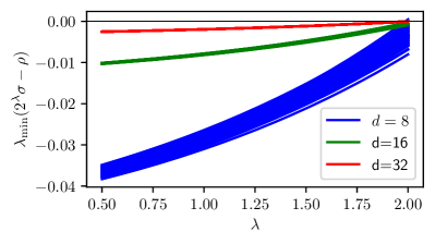
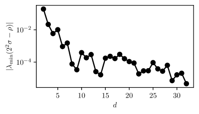
Figure 1: Minimal eigenvalue of matrix $2^{\lambda}\sigma-\rho$ as a function of $\lambda$ plotted for a fixed random $\rho$ of order $d^{2}$ and 100 randomly selected separable $\sigma$ (top) and a logarithmic plot of the absolute value of the maximum of these eigenvalues over 100 randomly chosen $\sigma$ and $\lambda=2$ as a function of dimension $d$ (bottom). As can be seen, the plots seem to justify the intuition behind the assumption $\lambda=2$ in the proof of Theorem 40.

The bound is loose as it has a non-vanishing factor of $2$. However, it is valid for any dimension of the shielding system of the state, and this factor is independent of the dimension. It implies that no matter how large is the shielding system of a key correlated state, generically, it brings in at most 2 bits of the repeated key above the (twice) one-way distillable entanglement.

It turns out, however, that there is a tighter bound, which can be obtained not from the upper bounding via relative entropy but squashed entanglement, Christandl and Müller-Hermes (2017); Tucci (2002). In the next section, we will show that the (half of) the mutual information of a random private state does not exceed the minimal value, which is key by more than $1\over 4$. The bound will then follow from a trivial inequality $R(\rho,\rho)^{\rightarrow}\leq R(\rho,\rho)\leq K_{D}(\rho)$ Bäuml et al. (2015).

IV Mutual information bound for the secure content of a random private bit

This section focuses on random private bits and provides an upper bound on the distillable key. We perform the random choice of a private state differently than it is done in Christandl et al. (2020). There, the private state has been first transformed via a one-way LOCC protocol to the form of the so-called Bell-private bit of the form $\frac{1}{2}\left(|\psi_{+}\rangle\langle\psi_{+}|\otimes\rho_{+}+|\psi_{-}\rangle\langle\psi_{-}|\otimes\rho_{-}\right)$. Then the two states were defined as $\rho_{\pm}:=U\bar{\rho}_{\pm}U$, where $\bar{\rho}_{\pm}$ is arbitrarily chosen state of the form $\bar{\rho}_{+}:=\frac{Q}{TrQ}$ with $Q$ being a projector onto any $d^{2}/2$ dimensional subspace of $A^{\prime}B^{\prime}$ system, and $\bar{\rho}_{-}:=\frac{Q^{\perp}}{TrQ^{\perp}}$. Our approach is different, as it also applies to the smallest dimension of the shield $d_{s}=2$. We do not transform a private bit into a Bell private bit. We rather observe that any private bit is uniquely represented by a (not necessarily normal) operator $X$ of trace norm equal to 1. We then represent this operator as $U\sigma$ and choose a random state $\sigma$ and random unitary $U$ according to the Haar measure.

Let us start by introducing the notion of random private states. Looking at Eq. (7) we have two objects that can be chosen at random: the unitaries $U_{0},U_{1}$ and the shared state $\sigma_{A^{\prime}B^{\prime}}$. Due to the unitary invariance of the ensemble of random quantum states, we can set one of the unitaries $U_{0}=\mathds{1}$ and the second one to be chosen randomly, denoted $U_{1}=U$. For simplicity, let us also introduce the notation $X=U\sigma_{A^{\prime}B^{\prime}}$. Hence, we can rewrite Eq. (7) as

$$\gamma_{ABA^{\prime}B^{\prime}}={1\over 2}\begin{pmatrix}\sqrt{XX^{\dagger}}&0&0&X\\ 0&0&0&0\\ 0&0&0&0\\ X^{\dagger}&0&0&\sqrt{X^{\dagger}X}\end{pmatrix}.$$ (43)

A short introduction into the properties of random unitaries and quantum states can be found in Appendix B. Before statement of the main result, which is the bound on the distillable key of a random private bit, let us first state the following technical fact

Proposition 1.

Let $\gamma_{ABA^{\prime}B^{\prime}}$ be defined as in Eq. (43), let $X$ be an arbitrary random matrix of dimension $d^{2}$ and let $\mu_{X}$ denote the asymptotic eigenvalue density of $\sqrt{XX^{\dagger}}$. Then, as $d\to\infty$, $\gamma$ has the eigenvalue density $\mu_{\gamma}$ given by

$$\mu_{\gamma}=\frac{1}{2}\mu_{X}+\frac{1}{2}\delta(0).$$ (44)

Proof.

From the form of $\gamma_{ABA^{\prime}B^{\prime}}$ we can conclude that half of its eigenvalues are equal to zero. Therefore it suffices to focus on the eigenvalues of the matrix

$$\gamma^{\prime}=\frac{1}{2}\begin{pmatrix}\sqrt{XX^{\dagger}}&X\\ X^{\dagger}&\sqrt{X^{\dagger}X}.\end{pmatrix}.$$ (45)

First we note that for any $\ket{\psi}$ we have

$$\gamma^{\prime}\begin{pmatrix}\ket{\psi}\\ -X^{\dagger}(\sqrt{XX^{\dagger}})^{-1}\ket{\psi}\end{pmatrix}=0.$$ (46)

Hence $\rank{\gamma^{\prime}}=d^{2}$, which gives us that half of the eigenvalues of $\gamma^{\prime}$ are equal to zero. From the fact that the Schur complement of the first block is $\gamma^{\prime}/\sqrt{XX^{\dagger}}=0$, we recover that the remaining eigenvalues of $\gamma^{\prime}$ are those of $\sqrt{XX^{\dagger}}$. ∎

Additionally, we will need the following fact regarding the entropy of random quantum states sampled from the Hilbert-Schmidt distribution from Bengtsson and Życzkowski (2017); Collins and Nechita (2011); Puchała et al. (2016); Życzkowski and Sommers (2001).

Proposition 2.

Let $\rho$ be a random mixed state of dimension $d$ sampled from the Hilbert-Schmidt distribution. Then, for large $d$ we have

$$\mathbb{E}\left(S(\rho)\right)=\log_{2}d-\frac{1}{2\ln 2}-O\left(\frac{\log_{2}d}{d}\right)$$ (47)

Proof.

For large $d$ it can be shown Życzkowski and Sommers (2001) that

$$\mathbb{E}(\operatorname{Tr}\rho^{k})=d^{1-k}\frac{\Gamma(1+2k)}{\Gamma(1+k)\Gamma(2+k)}\left(1+O\left(\frac{1}{d}\right)\right).$$ (48)

What remains is to note that

$$\mathbb{E}\left(S(\rho)\right)=-\lim_{k\to 1}\frac{\partial\operatorname{Tr}\rho^{k}}{\partial k},$$ (49)

and the desired results follows from direct calculations. ∎

The main result of this section can be formulated as the following theorem

Theorem 4.

Let $\gamma_{ABA^{\prime}B^{\prime}}$ be a private state defined as in Eq. (43), with the shielding system of dimension $d_{s}\otimes d_{s}$, let also $X=U\sigma_{A^{\prime}B^{\prime}}$, where $U$ is a Haar unitary be an arbitrary and $\rho$ is a random mixed state sampled from the Hilbert-Schmidt distribution. Then as $d\to\infty$ we get

$$I(AA^{\prime}:BB^{\prime})\to 2+\frac{1}{2\ln 2}.$$ (50)

Proof.

From Propositions 1 and 2 we have that the entropy of a random mixed state $\rho$ of dimension $d_{s}$ asymptotically behaves as $\log_{2}d_{s}-\frac{1}{2\ln 2}-O\left(\frac{\log_{2}d_{s}}{d_{s}}\right)$ we have

$$S(AA^{\prime}BB^{\prime})=2\log_{2}d_{s}-\frac{1}{2\ln 2}-O\left(\frac{\log_{2}d_{s}}{d_{s}^{2}}\right).$$ (51)

All is left is to consider the terms $S(AA^{\prime})$ and $S(BB^{\prime})$. First we observe that

$$\gamma_{AA^{\prime}}=\frac{1}{2}\begin{pmatrix}\operatorname{Tr}_{B}^{\prime}U\sigma_{A^{\prime}B^{\prime}}U^{\dagger}&0\\ 0&\operatorname{Tr}_{B}^{\prime}\sigma_{A^{\prime}B^{\prime}}\end{pmatrix},$$ (52)

and similarly for $\gamma_{BB^{\prime}}$. As the ensemble of random quantum states is unitarily invariant, $U\sigma_{A^{\prime}B^{\prime}}U^{\dagger}$ is also a random quantum state. Based on the results from Nechita et al. (2018) we have that the partial trace of a $d_{s}^{2}\times d_{s}^{2}$ random quantum state is almost surely the maximally mixed state. Hence

$$S(AA^{\prime})=S(BB^{\prime})=\log_{2}2d_{s}-o(1).$$ (53)

Putting all of these facts together we obtain the desired result

$$I(AA^{\prime}:BB^{\prime})\to 2\log_{2}2+\frac{1}{2\ln 2}.$$ (54)

∎

We have then immediate corollary

Corollary 3.

For a random private bit $\gamma_{2}$ of arbitrary large dimension of the shield, in the limit of large $d_{s}\rightarrow\infty$, there is

$$K_{D}(\gamma_{2})\leq\log_{2}2+\frac{1}{4\ln 2}$$ (55)

Proof.

We use the bound by squashed entanglement $E_{sq}(\rho):=\inf_{\rho_{ABE},Tr_{E}\rho_{ABE}=\rho_{AB}}\frac{1}{2}I(A:B|E)_{\rho_{ABE}}$ Christandl and Winter (2004), by noticing, that it is upper bounded by $\frac{1}{2}I(A:B)$ (we consider half of the bound on the mutual information given in (54)). ∎

For the private states, the above bound yields a tighter result, than the one given in Theorem 40. Indeed, since $E_{D}^{\rightarrow}(\rho)\geq 0$, the bound of Eq. (40) is at least $2$. However, the one-way repeater rate of a bipartite state $\rho_{AB}$ can not be larger than the distillable key $K_{D}(\rho_{AB})$ Bäuml et al. (2015). This is a trivial bound: any key-repeater protocol can be viewed as a particular LOCC protocol between $A$ and $B$. As such, it can not increase the initial amount of key in the cut $A:B$. We thus have for a generic private state $\gamma$ (not necessarily irreducible) a trivial bound

$$R^{\rightarrow}(\gamma_{2},\gamma_{2})\leq K_{D}(\gamma_{2})\leq$$

$$1+{1\over 4\ln 2}\approx 1+0.360674.$$ (56)

Let us note here that the bound is far from being small in contrast with the bound for the private state taken at random due to different randomization procedures proposed in Christandl et al. (2020). This is because our technique does not immediately imply that the private state has Hermitian $X$, nor that its positive and negative parts are random states. We believe, however, that the above bound can be made tighter.

V Localizable private randomness for a generic local independent state

In this section, we study the rates of private randomness that can be distilled from a generic independent bit. We base on the following idea. While (half of the) mutual information is merely a weak bound on the private key. This function reports the exact amount of private randomness content of quantum state in various scenarios Yang et al. (2019).

Let us recall here, that the local independent bit (in bipartite setting) has form

$$\alpha_{AA^{\prime}B^{\prime}}=\sum_{i,j=0}^{1}{1\over 2}|i\rangle\langle j|\otimes U_{i}\sigma_{A^{\prime}B^{\prime}}U_{j}^{\dagger}.$$ (57)

where $U_{i}$ are unitary transformations acting on system $A^{\prime}B^{\prime}$ and $\sigma$ is an arbitrary state on the latter system. We assume that the system $A^{\prime}B^{\prime}$ is of dimension $d_{s}\otimes d_{s}$. Hence, in the matrix form, it is as follows

$$\alpha_{AA^{\prime}B^{\prime}}={1\over 2}\left(\begin{array}[]{cc}\sqrt{XX^{\dagger}}&X\\ X^{\dagger}&\sqrt{X^{\dagger}X}\end{array}\right)$$ (58)

where $X=U_{0}\sigma_{A^{\prime}B^{\prime}}U_{1}$. As it was observed in the case of the private bit, we can safely assume that $U_{0}=\mathds{1}$, and $U_{1}$ is arbitrary because $\sigma_{A^{\prime}B^{\prime}}$ will be taken at random.

We give below the argument for the analysis of the entropy of system $AA^{\prime}$, used in the proof of the next theorem.

Proposition 3.

Consider $\alpha_{AA^{\prime}B^{\prime}}$ as in Eq. (58). Then, $\tr_{B^{\prime}}\alpha_{AA^{\prime}B^{\prime}}$ converges almost surely to the maximally mixed state as $d\to\infty$

$$\lim_{d\to\infty}\|2d\tr_{B^{\prime}}\alpha_{AA^{\prime}B^{\prime}}-I\|=0.$$ (59)

Moreover, we have

$$\|2d\tr_{B^{\prime}}\alpha_{AA^{\prime}B^{\prime}}-I\|=O(d^{-1})$$ (60)

Proof.

We start by proving the limit. The explicit form of the partial trace reads

$$\tr_{B^{\prime}}\alpha_{AA^{\prime}B^{\prime}}=\frac{1}{2}\begin{pmatrix}\tr_{B^{\prime}}\sigma_{A^{\prime}B^{\prime}}&\tr_{B^{\prime}}U_{0}\sigma_{A^{\prime}B^{\prime}}U_{1}^{\dagger}\\ \tr_{B^{\prime}}U_{1}\sigma_{A^{\prime}B^{\prime}}U_{0}^{\dagger}&\tr_{B^{\prime}}U_{0}\sigma_{A^{\prime}B^{\prime}}U_{0}^{\dagger}\end{pmatrix}.$$ (61)

We immediately note that the diagonal blocks are partial traces of independent random states. Hence from Nechita et al. (2018) we have that they almost surely converge to the maximally mixed state. Formally we have (only for the first block)

$$\lim_{d\to\infty}\|d\tr_{B^{\prime}}\sigma_{A^{\prime}B^{\prime}}-I\|=0$$ (62)

The remainder of this part of the proof follows from the proof of Proposition 1, substituting $X=\tr_{B^{\prime}}U_{0}\sigma_{A^{\prime}B^{\prime}}U_{1}^{\dagger}$ in Eq. (45) and following the reasoning shown there.

The result on convergence rate follows directly from considerations on the variance of the average eigenvalue of $\tr_{B^{\prime}}\alpha_{AA^{\prime}B^{\prime}}$, which are presented after Eq. (26) in Nechita et al. (2018). ∎

In what follows, we will show achievable rates of private randomness for a randomly chosen ibit. They are encapsulated in the following theorem.

Theorem 5.

Let $\alpha_{AA^{\prime}B^{\prime}}$ given by Eq. (57) be the randomly generated state by picking up random state $\sigma_{A^{\prime}B^{\prime}}$ and a unitary transformation $U_{1}$ due to Haar measure. Let also $R_{G}:=1+\frac{1}{2\ln 2}+O(\frac{\log d_{s}}{d_{s}^{2}})$. Then the following bounds are achievable.

1. for no communication and no noise,
   $R_{A}\leq R_{G}-o(1)$, when
   $\log d_{s}\geq\frac{1}{2\ln 2}+O(\frac{\log d_{s}}{d_{s}^{2}})-o(1)$ and
   $R_{A}\leq 1+\log d_{s}$ otherwise,
   $R_{B}\leq 1+\frac{1}{2\ln 2}-O(\frac{\log_{2}d_{s}}{d_{s}})$, when
   $\log_{2}d_{s}\geq 1+\frac{1}{2\ln 2}+O(\frac{\log_{2}d_{s}}{d_{s}})$ and
   $R_{B}\leq\log d_{s}$ otherwise.

2. for free noise, but no communication,
   $R_{A}\leq R_{G}-o(1)$,
   $R_{B}\leq 1+\frac{1}{2\ln 2}-O(\frac{\log_{2}d_{s}}{d_{s}}).$

3. for free noise and free communication,
   $R_{A},R_{B}\leq R_{G}$

4. for free communication but no noise,
   $R_{A}\leq R_{G}$ when
   $\log d_{s}\geq\frac{1}{2\ln 2}+O(\frac{\log_{2}d_{s}}{d_{s}^{2}})-o(1)$, and
   $R_{A}\leq 1+\log d_{s}+o(1)$ otherwise.
   $R_{B}\leq R_{G}$ when
   $\log_{2}d_{s}\geq 1+\frac{1}{2\ln 2}+O(\frac{\log d_{s}}{d_{s}})$
   $R_{B}\leq\log_{2}d_{s}-O(\frac{\log d_{s}}{d_{s}})$, otherwise.
   

Proof.

1. By Theorem 1, case $1$, the rate of private randomness reads $R_{A}=\log|AA^{\prime}|-\max\{0,S(AA^{\prime}|B^{\prime})\}$. This equals $\log|AA^{\prime}|-\max\{0,S(AA^{\prime}B^{\prime})-S(B^{\prime})\}$. When $S(B^{\prime})>S(AA^{\prime}B^{\prime})$, we have $R_{A}=\log 2d_{s}$, as the analysis is the same as for the private state (see Eq. (52)). On the other hand, if $S(B^{\prime})\leq S(AA^{\prime}B^{\prime})$ which happens for all high enough dimensions $d_{s}$, there is

   $$R_{A} =\log 2d_{s}-[(\log d_{s}^{2}-\frac{1}{2\ln 2}$$ (63)

   $$-O(\frac{\log d_{s}}{d_{s}^{2}}))-(\log d_{s}-o(1))]$$

   $$=1+\frac{1}{2\ln 2}+O(\frac{\log d_{s}}{d_{s}})-o(1).$$ (64)

   In the above we have used the fact, that $S(AA^{\prime}B^{\prime})$ for an independent state equals $S(AA^{\prime}BB^{\prime})$ for a corresponding private bit (i.e. generated by the same twisting $\tau$ and from the same state $\sigma$).

   We have further $R_{B}\leq\log|B^{\prime}|-\max\{0,S(B^{\prime}|AA^{\prime})\}=\log|B^{\prime}|-\max\{0,S(AA^{\prime}B^{\prime})-S(AA^{\prime})\}$. Let us consider first the case when $S(AA^{\prime}B^{\prime})\geq S(AA^{\prime})$ which holds for large enough $d_{s}$ i.e. whenever $\log_{2}d_{s}\geq 1+\frac{1}{2\ln 2}+O(\frac{\log_{2}d_{s}}{d_{s}^{2}})+O(\frac{\log_{2}d_{s}}{d_{s}})$, which is equivalent to $\log_{2}d_{s}\geq 1+\frac{1}{2\ln 2}+O(\frac{\log_{2}d_{s}}{d_{s}})$, due to the big O(.) notation. (If this condition is not met there is clearly $R_{B}=\log d_{s}-O(\frac{\log d_{s}}{d_{s}})$).

   By asymptotic continuity of the von-Neumann entropy Winter (2016) and Proposition 3 we have $|S(AA^{\prime})-\log_{2}2d_{s}|\leq O(\frac{\log_{2}d_{s}}{d_{s}})+O(d_{s}^{-1})=O(\frac{\log_{2}d_{s}}{d_{s}})$ while $S(AA^{\prime}B^{\prime})=(\log_{2}d_{s}^{2}-\frac{1}{2\ln 2}-O(\frac{\log_{2}d_{s}}{d_{s}^{2}}))$ as argued above. To show achievability, we need to use the lower bound: $S(AA^{\prime})\geq\log_{2}2d_{s}-O(\frac{\log_{2}d_{s}}{d_{s}})$. We then obtain that $R_{B}\leq 1+\frac{1}{2\ln 2}-O(\frac{\log_{2}d_{s}}{d_{s}}))\leq\log_{2}|B^{\prime}|-S(B^{\prime}|AA^{\prime})$ is an achievable rate. Here we have included term $O(\frac{\log d_{s}}{d_{s}^{2}}))$ in term $O(\frac{\log_{2}d_{s}}{d_{s}}))$ due to the big $O(.)$ notation.

2. The second case reads the same bounds as the first just without additional conditions on dimension $d_{s}$. This is because in the second case of Theorem 1, the bounds have $S(A|B)$ and $S(B|A)$ terms rather than the $S(A|B)_{+}$ and $S(B|A)_{+}$ in its formulation.

3. The third case stems from an observation, that the global purity reads $R_{G}=\log|AA^{\prime}B^{\prime}|-S(AA^{\prime}B^{\prime})=\log(2d_{s}^{2})-(2\log d_{s}-\frac{1}{2\ln 2}-O(\frac{\log d_{s}}{d_{s}^{2}}))$. The rates $R_{A}$ and $R_{B}$ achive the same bound $R_{G}$ in this case.

4. The last case is due to case $4$ of the Theorem 1: $R_{A}\leq\log|AA^{\prime}B^{\prime}|-\max\{S(B^{\prime}),S(AA^{\prime}B^{\prime})\}$. When $S(B^{\prime})>S(AA^{\prime}B^{\prime})$ i.e. $\log d_{s}<\frac{1}{2\ln 2}+O(\frac{\log_{2}d_{s}}{d_{s}^{2}})-o(1)$, there is $R_{A}\leq 1+2\log_{2}d_{s}-\log_{2}d_{s}+o(1)=1+\log_{2}d_{s}+o(1)$. When $S(B^{\prime})\leq S(AA^{\prime}B^{\prime})$ there is $R_{A}\leq 1+2\log_{2}d_{s}-[2\log_{2}d_{s}-(\frac{1}{2\ln 2}+O(\frac{\log_{2}d_{s}}{d_{s}^{2}})])=1+\frac{1}{2\ln 2}+O(\frac{\log_{2}d_{s}}{d_{s}^{2}})$.

   Finally we have $R_{B}\leq\log|AA^{\prime}B^{\prime}|-\max\{S(AA^{\prime}),S(AA^{\prime}B^{\prime})\}$. When $\log_{2}d_{s}\geq 1+\frac{1}{2\ln 2}+O(\frac{\log d_{s}}{d_{s}})$ we have $S(AA^{\prime})\leq S(AA^{\prime}B^{\prime})$, and then $R_{B}\leq R_{G}=1+2\log d_{s}-(2\log d_{s}-\frac{1}{2\ln 2}-O(\frac{\log d_{s}}{d_{s}^{2}}))=1+\frac{1}{2\ln 2}+O(\frac{\log d_{s}}{d_{s}^{2}})$. Otherwise (if. $S(AA^{\prime})>S(AA^{\prime}B^{\prime})$) there is $R_{B}\leq 1+2\log d_{s}-(\log 2d_{s}+O(\frac{\log d_{s}}{d_{s}}))=\log d_{s}-O(\frac{\log d_{s}}{d_{s}})$.

∎

From the above Theorem we can see that in case of the system $A$, for asymptotically large dimension $d_{s}$ the value of global purity $1+\frac{1}{2\ln 2}+O(\frac{\log d_{s}}{d_{s}^{2}})$ can be reached in all four cases. In the case of system $B$ we invoked only the (lower and upper) bounds on the entropy of involved systems ($AA^{\prime}$), hence the bounds are not tight, possibly less than the maximal achievable ones.

VI Discussion

We have generalized bound by M. Christandl and R. Ferrara Christandl and Ferrara (2017) to the case of arbitrary key correlated states. We then show a sequence of relaxation of this bound, from which it follows that the repeated key of a key correlated state can not be larger from one-way distillable entanglement than by twice the max-relative entropy of its attacked state.

We further ask how big is the key content of a random private bit, which need not be irreducible Horodecki et al. (2018). A not irreducible private bit can have more distillable key than $1$. It turned out that the amount of key is bounded by a constant factor independent of the dimension of the shielding system. It is interesting if the constant $\approx 0.36$ can be improved. One could also ask if this randomization technique also results in a state for which the repeated key is vanishing with large dimension of the shield as it was shown by a different technique of randomization in Christandl et al. (2020). Recent results on private randomness generation Yang et al. (2019) let us also estimate the private randomness content of generic independent bits. Generalizing this result for independent states of larger dimensions would be the next important step.

We also show a bound on the distillable key based on the techniques developed in this manuscript. The bound can not be better than the bound by $E_{R}$. However, it can possibly report how the relative entropy distance deviates from being a metric. Indeed, our bound is in terms of a ’proxy’ arbitrary state. Indeed, we have two terms: $\frac{\alpha}{1-\alpha}D(\rho||\rho^{\prime})$ and ${\tilde{D}}_{\alpha}(\rho^{\prime}||\sigma)$ where $\rho^{\prime}$ is some intermediate state between $\rho$ and separable state $\sigma$. One could believe that the bound is non-trivial, as the relative entropy functions involved are not metrics. In particular, the triangle inequality reporting that going via proxy state yields a larger result does not hold. However, we know anyway that the bound can not be better than the one by $E_{R}$ itself, hence, conversely, we can perhaps conclude from the bound, how far are the relative entropy functions from being a metric.

Finally, we would like to stress that our approach is generic. That is, it appears that any other strong-converse bound on the quantum distillable key may give rise to a new, possibly tighter bound on the one-way quantum key repeater rate. Hence recent strong-converse bound on quantum privacy amplification Salzmann and Datta (2022) paves the way for future research in this direction. It would be important to extend this technique for the two-way quantum key repeater rate.

Appendix A Bound for distillable key

We derive now a novel form of a bound on the distillable key in terms of relative entropy functions. Although the bound reduces to a well-known bound $K_{D}\leq E_{R}$ Horodecki et al. (2005, 2009a), we state it due to its novelty. The novelty comes from the fact that it involves the relative entropy distance from arbitrary, not necessarily separable, quantum state. The main result is encapsulated in Theorem 72 below.

We first focus on the analogue of Lemma 1 and Lemma 2 for the key distillation rather than repeated key distillation. The abstract version of the Lemma 1 reads

Lemma 3.

For a bipartite state of the form $\tilde{\sigma}:=\operatorname{Tr}_{A^{\prime}B^{\prime}}U\sigma_{ABA^{\prime}B^{\prime}}U^{\dagger}$, where $\sigma_{ABA^{\prime}B^{\prime}}$ is arbitrary state and $U$ is a twisting, there is

$$\operatorname{Tr}\tilde{\sigma}\psi_{+}^{\otimes m}\leq 2^{-(\frac{\alpha-1}{\alpha})[m-\tilde{E}_{\alpha}(\sigma)]},$$ (65)

where $m\geq 1$ is a natural number, $\psi_{+}$ denotes the maximally entangled state, and $\alpha\in(1,\infty)$.

Proof.

As in the proof of the Lemma 1, we directly use the proof of the strong-converse bound for the distillable key of Das et al. (2021) which is based on Das et al. (2020); Christandl and Müller-Hermes (2017). Let us suppose $\operatorname{Tr}\tilde{\sigma}\psi_{+}^{\otimes m}=1-\epsilon$. Let us also choose a state $\hat{\sigma}$, to be a twisted separable state of the form. $\hat{\sigma}=\operatorname{Tr}_{A^{\prime}B^{\prime}}U\sigma_{AA^{\prime}:BB^{\prime}}^{\prime}U^{\dagger}$ with $\sigma^{\prime}$ being arbitrary separable state in $(AA^{\prime}:BB^{\prime})$ cut. Since any such state has overlap with the singlet state $\psi^{\otimes m}_{+}$ less than $\frac{1}{2^{m}}\equiv 1/K$ (see lemma 7 of Horodecki et al. (2009a)), we have:

$$D^{\epsilon}_{h}(\tilde{\sigma}||\hat{\sigma})\geq\log_{2}K=m$$ (66)

and further for any $\alpha\in(1,\infty)$

$$\tilde{D}_{\alpha}(\tilde{\sigma}||\hat{\sigma})+\frac{\alpha}{\alpha-1}\log_{2}(\frac{1}{1-\epsilon})=$$

$$\tilde{D}_{\alpha}(\operatorname{Tr}_{A^{\prime}B^{\prime}}U\sigma U^{\dagger}||\operatorname{Tr}_{A^{\prime}B^{\prime}}U\sigma^{\prime}_{A:B}U^{\dagger})+$$

$$\frac{\alpha}{\alpha-1}\log_{2}(\frac{1}{1-\epsilon})\geq m$$ (67)

we can now relax $\tilde{\sigma}$ to $\sigma$ due to monotonicity of the sandwich R$\acute{e}$nyi relative entropy distance under jointly applied channel, so that

$$\tilde{D}_{\alpha}(\sigma||\sigma^{\prime})+\frac{\alpha}{\alpha-1}\log_{2}(\frac{1}{1-\epsilon})\geq m$$ (68)

Since $\sigma^{\prime}$ is an arbitrary separable state, we can take also the infimum over this set obtaining:

$$\tilde{E}_{\alpha}(\sigma)+\frac{\alpha}{\alpha-1}\log_{2}(\frac{1}{1-\epsilon})\geq m.$$ (69)

We can now rewrite it as follows:

$$1-\epsilon\leq 2^{-(\frac{\alpha-1}{\alpha})(m-E_{\alpha}(\sigma))}$$ (70)

Since $1-\epsilon=\operatorname{Tr}\tilde{\sigma}\psi_{+}^{\otimes m}$, the assertion follows. ∎

Lemma 4.

For a maximally entangled state $\psi_{+}^{\otimes m}$, a state $\tilde{\sigma}:=\operatorname{Tr}_{A^{\prime}B^{\prime}}U\sigma U^{\dagger}$ where $U$ is a twisting, for every $\alpha\in(1,\infty)$, there is

$$E_{R}^{\mbox{Cone}(\tilde{\sigma})}(\psi_{+}^{Rn})\equiv$$

$$\inf_{\sigma\in\mbox{Cone}(SEP,\tilde{\sigma})}D(\psi_{+}^{Rn}||\sigma_{n})\geq(\frac{\alpha-1}{\alpha})(m-E_{\alpha}(\sigma)).$$ (71)

Proof.

The proofs goes in full analogy to the proof of Lemma 2. ∎

Theorem 6.

For every bipartite state $\rho\in{\cal B}({\cal C}^{d_{A}}\otimes{\cal C}^{d_{B}})\equiv{\cal H}$, there is:

$$K_{D}(\rho)\leq\inf_{\sigma\in{\cal H},\alpha\in(1,\infty]}[\frac{\alpha}{\alpha-1}D(\rho||\sigma)+\tilde{E}_{\alpha}^{\infty}(\sigma)]$$ (72)

Proof.

The proof goes along the line of the proof of the fact that $E_{R}$ is the upper bound on distillable key $K_{D}$ Horodecki et al. (2005, 2009a). Let the LOCC protocol $\Lambda$ distill a state close by $\epsilon>0$ to a private state $\gamma_{m}$ with $m$-qubit key part, when acting on $n$ copies of $\rho$. Let us also denote $m=nR$ where $R>K_{D}(\rho)-\eta$ by some $\eta>0$. We will show the chain of (in)equalities and comment them below:

$$D(\rho||\sigma)={1\over n}D(\rho^{\otimes n}||\sigma^{\otimes n})\geq$$ (73)

$${1\over n}D(\Lambda(\rho^{\otimes})||\Lambda(\sigma^{\otimes n}))\geq$$ (74)

$${1\over n}D(\operatorname{Tr}_{A^{\prime}B^{\prime}}U\Lambda(\rho^{\otimes})U^{\dagger}||\operatorname{Tr}_{A^{\prime}B^{\prime}}U\Lambda(\sigma^{\otimes n})U^{\dagger})\equiv$$

$${1\over n}D(\operatorname{Tr}_{A^{\prime}B^{\prime}}U\Lambda(\rho^{\otimes})U^{\dagger}||\sigma_{n})\geq$$ (75)

$${1\over n}\inf_{\tilde{\sigma}_{n}\in Cone(SEP,\sigma_{n})}D(\tilde{\psi}_{+}^{\otimes m}||\tilde{\sigma}_{n})\geq$$ (76)

$$\inf_{\tilde{\sigma}_{n}\in Cone(SEP,\sigma_{n})}D(\psi_{+}^{\otimes m}||\tilde{\sigma}_{n})+{1\over n}O(\epsilon+h(\epsilon))\geq$$ (77)

$${1\over n}[n\frac{\alpha-1}{\alpha}(R-{1\over n}\tilde{E}_{\alpha}(\sigma^{\otimes n})]+{1\over n}O(\epsilon+h(\epsilon))$$ (78)

In the first step, we use the tensor-property of the relative entropy. In the next, we use monotonicity of the relative entropy under $\Lambda$, and further under a map which consists of untwisting by $U$ and tracing out system $A^{\prime}B^{\prime}$. The twisting $U$ is defined by $\gamma_{m}$. We further relax relative entropy to infimum over states from $Cone(SEP,\sigma_{n})$ to which $\sigma_{n}$ belongs to, and use asymptotic continuity of the relative entropy from a convex set. We then use the analogue of Lemma 2.

Taking the limit of $n$ going to infinity, $\eta\rightarrow 0$ and $\epsilon\rightarrow 0$ proves the thesis. ∎

Remark 1.

The bound of Eq. (72) has two extreme cases. First is when we set $\sigma=\rho$. In that case the first term equals zero because $D(\rho||\rho)=0$, and the second term equals $\tilde{E}_{\alpha}(\rho)$, where $\alpha>1$. Taking limit $\alpha\rightarrow 1$, we obtain a known bound $E_{R}(\rho)$ on distillable key. The second extreme is when we set $\sigma$ to be any separable state. Then the second term is zero as $\tilde{E}_{\alpha}$ is the relative entropy divergence ”distance” from the set of separable states. In that case, we can take the limit $\alpha\rightarrow\infty$, and again obtain the bound $E_{R}(\rho)$.

Appendix B Random quantum objects

In this section we provide a short introduction into random matrices. The scope is limited to concepts necessary in the understanding of our result.

B.1 Ginibre matrices

We start of by introducing the Ginibre random matrices ensemble Ginibre (1965). This ensemble is at the core of a vast majority of algorithms for generating random matrices presented in later subsections. Let $(G_{ij})_{1\leq i\leq m,1\leq j\leq n}$ be a $m\times n$ table of independent identically distributed (i.i.d.) random variable on $\mathbb{C}$. The field $\mathbb{K}$ can be either of $\mathbb{R}$, $\mathbb{C}$ or $\mathbb{Q}$. With each of the fields we associate a Dyson index $\beta$ equal to $1$, $2$, or $4$ respectively. Let $G_{ij}$ be i.i.d random variables with the real and imaginary parts sampled independently from the distribution $\mathcal{N}(0,\frac{1}{\beta})$. Hence, $G\in\mathrm{L}(\mathcal{X},\mathcal{Y})$, where matrix $G$ is

$$P(G)\propto\exp(-\operatorname{Tr}GG^{\dagger}).$$ (79)

This law is unitarily invariant, meaning that for any unitary matrices $U$ and $V$, $G$, and $UGV$ are equally distributed. It can be shown that for $\beta=2$ the eigenvalues of $G$ are uniformly distributed over the unit disk on the complex plane Tao and Vu (2008).

B.2 Wishart matrices

Wishart matrices form an ensemble of random positive semidefinite matrices. They are parametrized by two factors. First is the Dyson index $\beta$ which is equal to one for real matrices, two for complex matrices and four for symplectic matrices. The second parameter, $K$, is responsible for the rank of the matrices. They are sampled as follows

1. Choose $\beta$ and $K$.

2. Sample a Ginibre matrix $G\in\mathrm{L}(\mathcal{X},\mathcal{Y})$ with the Dyson index $\beta$ and $\mathrm{dim}(\mathcal{X})=d$ and $\mathrm{dim}(\mathcal{Y})=Kd$.

3. Return $W=GG^{\dagger}$.

Sampling this ensemble of matrices will allow us to sample random quantum states. This process will be discussed in further sections. Aside from their construction, we will not provide any further details on Wishart matrices, as this falls outside the scope of this work.

B.3 Circular unitary ensemble

Circular ensembles are measures on the space of unitary matrices. Here, we focus on the circular unitary ensemble (CUE), which gives us the Haar measure on the unitary group. In the remainder of this section, we will introduce the algorithm for sampling such matrices.

There are several possible approaches to generating random unitary matrices according to the Haar measure. One way is to consider known parametrizations of unitary matrices, such as the Euler Życzkowski and Kuś (1994) or Jarlskog Jarlskog (2005) ones. Sampling these parameters from appropriate distributions yields a Haar random unitary. The downside is the long computation time, especially for large matrices, as this involves a lot of matrix multiplications. We will not go into this further; instead, we refer the interested reader to the papers on these parametrizations.

Another approach is to consider a Ginibre matrix $G\in\mathrm{L}(\mathcal{X})$ and its polar decomposition $G=UP$, where $U\in\mathrm{L}(\mathcal{X})$ is unitary and $P$ is a positive matrix. The matrix $P$ is unique and given by $\sqrt{G^{\dagger}G}$. Hence, assuming $P$ is invertible, we could recover $U$ as

$$U=G(G^{\dagger}G)^{-\frac{1}{2}}.$$ (80)

As this involves the inverse square root of a matrix, this approach can be potentially numerically unstable.

The optimal approach is to utilize the QR decomposition of $G$, $G=QR$, where $Q\in\mathrm{L}(\mathcal{X})$ is unitary and $R\in\mathrm{L}(\mathcal{X})$ is upper triangular. This procedure is unique if $G$ is invertible and we require the diagonal elements of $R$ to be positive. As typical implementations of the QR algorithm do not consider this restriction, we must enforce it ourselves. The algorithm is as follows

1. Generate a Ginibre matrix $G\in\mathrm{L}(\mathcal{X})$, $\mathrm{dim}(\mathcal{X})=d$

2. Perform the QR decomposition obtaining $Q$ and $R$.

3. Multiply the $i$^th column of $Q$ by $r_{ii}/|r_{ii}|$.

This gives us a Haar distributed random unitary. For a detailed analysis of this algorithm, see Mezzadri (2007). This procedure can be generalized in order to obtain a random isometry. The only required change is the dimension of $G$. We simply start with $G\in\mathrm{L}(\mathcal{X},\mathcal{Y})$, where $\dim(\mathcal{X})\geq\dim(\mathcal{Y})$.

B.4 Random mixed quantum states

In this section, we discuss the properties and methods of generating mixed random quantum states.

Random mixed states can be generated in one of two equivalent ways. The first one comes from the partial trace of random pure states. Suppose we have a pure state $\ket{\psi}\in\mathcal{X}\otimes\mathcal{Y}$. Then we can obtain a random mixed as

$$\rho=\tr_{\mathcal{Y}}\outerproduct{\psi}{\psi}.$$ (81)

Note that in the case $\dim(\mathcal{X})=\dim(\mathcal{Y})$ we recover the (flat) Hilbert-Schmidt distribution on the set of quantum states.

An alternative approach is to start with a Ginibre matrix $G\in\mathrm{L}(\mathcal{X},\mathcal{Y})$. We obtain a random quantum state $\rho$ as

$$\rho=GG^{\dagger}/\operatorname{Tr}(GG^{\dagger}).$$ (82)

It can be easily verified that this approach is equivalent to the one utilizing random pure states. First, note that in both cases, we start with $\dim(\mathcal{X})\dim(\mathcal{Y})$ complex random numbers sampled from the standard normal distribution. Next, we only need to note that taking the partial trace of a pure state $\ket{\psi}$ is equivalent to calculating $AA^{\dagger}$ where $A$ is a matrix obtained from reshaping $\ket{\psi}$.

The properties of these states have been extensively studied. We will omit stating all the properties here and refer the reader to Wootters (1990); Życzkowski and Sommers (2001); Sommers and Życzkowski (2004); Puchała et al. (2016); Zhang et al. (2017); Zhang (2017).