∎

e1e-mail: breoni@hhu.de

We study a one-dimensional three-state run-and-tumble model motivated by the bacterium Caulobacter crescentus which displays a cell cycle between two non-proliferating mobile phases and a proliferating sedentary phase. Our model implements kinetic transitions between the two mobile and one sedentary states described in terms of their number densities, where mobility is allowed with different running speeds in forward and backward direction. We start by analyzing the stationary states of the system and compute the mean and squared-displacements for the distribution of all cells, as well as for the number density of settled cells. The latter displays a surprising super-ballistic scaling $\sim t^{3}$ at early times. Including repulsive and attractive interactions between the mobile cell populations and the settled cells, we explore the stability of the system and employ numerical methods to study structure formation in the fully nonlinear system. We find traveling waves of bacteria, whose occurrence is quantified in a non-equilibrium state diagram.

A one-dimensional three-state run-and-tumble model with a ‘cell cycle’

1 Introduction

Understanding the motion of bacteria has been a classic problem of biophysics berg_e_2004 ; berg_random_2018 . Bacteria are propelled by their flagellae, whose motor generates a torque which translates into forward or backward motion of the bacteria. The problem has also found interest within the soft matter community, as bacteria are but one example of a much larger class of systems, commonly denoted as microswimmers elgeti_physics_2015 . The run-and-tumble (RT) model of an active particle system is originally motivated by specific features of bacterial motion: this motion only persists for a finite time, the ‘run’-time, after which the bacterium stalls, the ‘tumble’-period, before continuing its motion typically in a different direction, see e.g. polin_chlamydomonas_2009 . The properties of the basic RT model have been confronted with experiments, e.g. in detcheverry_generalized_2017 ; fier_langevin_2018 . The RT model also relates to other stochastic processes, e.g. the exclusion process bertrand_dynamics_2018 or even to the dynamics of quantum particles maes_diffraction_2022 .

RT models in one dimension are a special case within this model class. Here, the bacterium can only switch between left- and right motion in a stochastic manner. One-dimensional RT-models have proven to be an extremely rich field for analytic calculations; exemplary papers dealing with diverse aspects are: confinement angelani_confined_2017 ; space-dependent velocities, space-dependent transition rates and general drift velocity distributions angelani_run-and-tumble_2019 ; dhar_run-and-tumble_2019 ; singh_local_2021 ; monthus_large_2021 ; frydel_generalized_2021 ; hard-core particles with spin dandekar_hard_2020 ; inhomogeneous media singh_run-and-tumble_2020 ; attractive/repulsive interactions le_doussal_stationary_2021 ; barriusogutierrez_collective_2021 ; phase transitions mori_first-order_2021 ; entropy production frydel_intuitive_2022 . Field-theoretic methods have been applied to RT models recently as well garcia-millan_run-and-tumble_2021 ; zhang_field_2022 .

In some sense, the (one-dimensional) RT model can be thought of playing in active systems a role analogous to Ising models in equilibrium statistical mechanics. In the very recent past, several works have appeared carrying this analogy further, since they consider the number of ‘states’ in which the bacterium can find itself to go beyond the dichotomy of left- and right-moving states. Models with three and even more states have been discussed - in our Ising-model analogy, this amounts to looking at active analogues of ‘Potts’-type models basu_exact_2020 ; grange_run-and-tumble_2021 ; frydel_run-and-tumble_2022 .

The present paper inserts itself in this line of research by considering a three-state RT model with the states: left-moving, right-moving and sedentary. Our model is motivated by the behavior of the bacterium Caulobacter crescentus (CC), a model organism in microbiology since it has a complex lifestyle shebelut_caulobacter_2010 ; biondi_cell_2022 . CC has a bacterial analogue of a cell cycle usually found in eukaryotes; in order to undergo cell division, the bacterium has to switch from its mobile swarmer state to a spatially localized stalked state. Only from the latter state the proliferation of new cells is possible. Our model, capturing this biological feature, is however not limited to CC or bacteria alone. E.g., the green algae Chlamydomonas reinhartii has a similar cell cycle harris_chlamydomonas_2009 with sedentary and swimming states and also performs a run-and-tumble motion polin_chlamydomonas_2009 . The capacity of cell division in our RT model inks it to the problem of the growth of bacterial colonies. Recently, the authors of narla_traveling-wave_2021 developed a growth-expansion model which generates traveling waves in bacterial chemotaxis, in accord with experimental observations. We show that traveling waves also arise in our much simpler 1d run-and-tumble model.

The paper is organized as follows. In Section 2, we introduce our RT-model as a toy model, inspired by the cell cycle of CC. In Section 3, we first focus on the case of free cells for which we derive the conditions for stability of the system when spatial dependencies are neglected. In Section 4 we consider the spatial dependence built into the model and study the mean displacement (MD) and mean squared displacement (MSD) for a single cell in the process of duplicating, both showing a surprising $t^{3}$ regime for short times. Allowing the cells to interact via both attraction and repulsion mechanisms, this antagonistic effect is found to lead to structure formation: we numerically find traveling wave solutions of the system density and quantify their occurrence in a non-equilibrium state diagram. Finally we discuss how the model performs with parameter values specific of CC. Section 5 concludes the paper with a discussion of the results of our model and a brief outlook on further work.

2 The model

Inspired by the reproductive behavior of Caulobacter crescentus we consider a one-dimensional toy model representing bacteria that can actively move rightward, leftward or settle down, and that when settled double in number. We note, that CC performs a run-reverse-flick motion grognot_more_2021 , where the bacterium first performs a forward motion, then reverses its direction of motion and in a third step makes a turn mediated by a buckling instability in its flagellum son_bacteria_2013 . Since our setup is one dimensional, the run-reverse-flick motion is equivalent to a run and tumble motion.

The ‘cell cycle’ of our three-state RT model motivated by CC is summarized in Figure 1. We allow for three populations with the number densities $\rho_{+}(x,t)$, $\rho_{-}(x,t)$ and $\rho_{0}(x,t)$, functions of space $x$ and time $t$, respectively corresponding to right and left movers, and to the sedentary population. The ‘cell cycle’ step is given by the rate of settling down, $\lambda_{s}$, which can occur from either moving state, and the cell doubling with rate $\lambda_{d}$ with which a sedentary bacterium gives rise to a pair of right- and left-moving cells. The exchange of direction, i.e. the RT step, is denoted by $\lambda_{e}$. Finally, $\mu$ is the death rate, which we consider for motile cells only. In a proliferating system, this rate prevents exponential growth.

Figure 1: Graphical representation of the transition rates among different species. These transitions are motivated by the cell cycle of Caulobacter crescentus, that either moves actively or settles down to reproduce. Our model contains three different species: the cells moving to the right $\rho_{+}$, those moving to the left $\rho_{-}$ and the settled ones $\rho_{0}$. The moving cells can either settle via the rate $\lambda_{s}$, move in the opposite direction with $\lambda_{e}$ or die with $\mu$. Settled cells duplicate via $\lambda_{d}$, and generate both a left- and a right-moving cell.

This idealized CC-‘cell cycle’ is implemented in terms of evolution equations for the cell number densities. In the case where there is no death or proliferation, the number densities can also be interpreted as probability densities and the evolution equations correspond to Fokker-Planck equations.

As the bacteria are micron-sized swimmers, we assume a low Reynolds number and overdamped dynamics. To describe this behavior mathematically we first group the three densities into the vector of densities $\boldsymbol{\rho}=(\rho_{+},\rho_{0},\rho_{-})$. The dynamics of the system will then be described by the differential equation

$$\partial_{t}\boldsymbol{\rho}={\mathcal{D}}\partial_{x}^{2}\boldsymbol{\rho}+\partial_{x}[(\partial_{x}{\mathcal{U}})\cdot\boldsymbol{\rho}]-{\cal V}\cdot\partial_{x}\boldsymbol{\rho}+{\cal M}\boldsymbol{\rho}$$ (1)

which generalizes the standard expression of growth-expansion equations of logistic growth, usually formulated for a single density narla_traveling-wave_2021 . In Eq. (1), the first term is a diffusion term where the matrix ${\cal D}$ has the form

$$\mathcal{D}=\begin{pmatrix}D&0&0\\ 0&0&0\\ 0&0&D\end{pmatrix}$$ (2)

since the sedentary particles do not diffuse. The second term on the right-hand side is a nonlinear diffusion coefficient containing an interaction matrix ${\cal U}$ of the form

$$\mathcal{U}=\begin{pmatrix}-\kappa\rho_{0}&0&0\\ 0&\kappa_{0}\rho_{0}&0\\ 0&0&-\kappa\rho_{0}\end{pmatrix}\,.$$ (3)

The matrix entries describe attractive interactions (negative sign) of the moving cells to regions in which particles have settled and repulsive interactions among settled cells (positive sign) in order to mimic biofilm behaviour. The third term on the right-hand side of Eq. (1) describes the active motion of the particles in the right and left directions along the line. Hence

$$\mathcal{V}=\begin{pmatrix}v_{+}&0&0\\ 0&0&0\\ 0&0&-v_{-}\end{pmatrix}\,.$$ (4)

Finally, we have for the cell cycle or population dynamics part, following the transitions shown in Figure 1, the matrix ${\cal M}$ given by

$$\mathcal{M}=\begin{pmatrix}-(\lambda_{s}+\lambda_{e}+\mu)&\lambda_{d}&\lambda_{e}\\ \lambda_{s}&-\lambda_{d}&\lambda_{s}\\ \lambda_{e}&\lambda_{d}&-(\lambda_{s}+\lambda_{e}+\mu)\end{pmatrix}\,.$$ (5)

Given that our run-and-tumble model allows for proliferation and death of cells, it is important to recognize that the population dynamics of Eq. (1) is the linear limit of the more general nonlinear decay-growth equation

$$\partial_{t}\boldsymbol{\rho} = {\mathcal{D}}\partial_{x}^{2}\boldsymbol{\rho}+\partial_{x}[(\partial_{x}{\mathcal{U}})\cdot\boldsymbol{\rho}]-{\cal V}\cdot\partial_{x}\boldsymbol{\rho}$$ (6)

$$+\mathcal{M}_{D}\boldsymbol{\rho}+\mathcal{M}_{OD}\boldsymbol{\mathcal{R}}(\boldsymbol{\rho}).$$

In Eq. (6), $\mathcal{M}_{D}$ and $\mathcal{M}_{OD}$ are the diagonal and off-diagonal parts of the matrix $\mathcal{M}$, i.e., one has $\mathcal{M}=\mathcal{M}_{D}+\mathcal{M}_{OD}$. The diagonal part describes the cell number decay, while the off-diagonal part describes the growth of the cell population. In order to limit growth, the non-diagonal term is generally nonlinear and saturating at the carrying capacity, as is common in growth-expansion models, see, e.g. narla_traveling-wave_2021 . The vector $\mathcal{R}$ is thus given by

$$\boldsymbol{\mathcal{R}}=\begin{pmatrix}\rho_{+}(1-\frac{\rho_{+}}{\rho_{+,c}})\\ \rho_{0}(1-\frac{\rho_{0}}{\rho_{0,c}})\\ \rho_{-}(1-\frac{\rho_{-}}{\rho_{-,c}})\end{pmatrix}\,.$$

where the carrying capacity is given by the vector

$${\boldsymbol{\rho}}_{c}(x)\equiv\left(\rho_{+,c}(x),\rho_{0,c}x),\rho_{-,c}(x)\right)\,.$$ (7)

The linear limit of Eq. (6) is reached for $|\boldsymbol{\rho}|\ll|\boldsymbol{\rho}_{c}|$. It is important to notice that since $\mathcal{R}$ is only applied to one part of the $\mathcal{M}$ matrix, the stationary values reached by the population in the linear limit will not necessarily be those given by $\boldsymbol{\rho}_{c}$. The main benefit of the nonlinear model is that it prevents the number of cells from exploding independently of the parameters. In this manuscript we will mainly focus on the linear case, while explicitly referring to the full nonlinear growth equation if needed.

3 Free cells

We start by setting the cell interaction parameters $\kappa=\kappa_{0}=0$, and hence consider free cells.

3.1 Population dynamics

In this section we further set $D=0$ as well as the velocities $v_{+}=v_{-}=0$, thus we first study free cells undergoing the pure population dynamics given by

$$\partial_{t}\boldsymbol{\rho}(x,t)={\cal M}\boldsymbol{\rho}(x,t)\,.$$ (8)

This linear system of equations can be solved analytically via matrix calculations, leading to

$$\boldsymbol{\rho}(x,t)=\text{e}^{\mathcal{M}t}\boldsymbol{\rho}(x,0)=\mathcal{P}\text{e}^{\mathcal{E}t}\mathcal{P}^{-1}\boldsymbol{\rho}(x,0).$$ (9)

$\mathcal{P}$ is the eigenvector matrix of $\mathcal{M}$ and $\mathcal{E}$ is the diagonal matrix containing the eigenvalues of $\mathcal{M}$, that are

$$\mathcal{E}_{1}= -(\mu+2\lambda_{e}+\lambda_{s})$$

$$\mathcal{E}_{2}= -(\mu+\lambda_{d}+\lambda_{s}+\Lambda)/2\$$ (10)

$$\mathcal{E}_{3}= -(\mu+\lambda_{d}+\lambda_{s}-\Lambda)/2,$$

where $\Lambda=\sqrt{(\mu+\lambda_{d}+\lambda_{s})^{2}+4\lambda_{d}(\lambda_{s}-\mu)}$. We notice that the first two eigenvalues are always negative and therefore stable, while the sign of the third depends on $\lambda_{s}-\mu$, which can become unstable. This instability facilitates an exponential growth of the colony. In fact, for small values of $\lambda_{d}(\lambda_{s}-\mu)$ with respect to $\mu+\lambda_{d}+\lambda_{s}$ the unstable eigenvalue becomes

$$\mathcal{E}_{3}\simeq\frac{\lambda_{d}(\lambda_{s}-\mu)}{\mu+\lambda_{d}+\lambda_{s}}.\\$$ (11)

The exponential growth or collapse of the system is therefore decided by the difference of $\lambda_{s}$ and $\mu$, or in different terms, the separating line between the two behaviors is $\lambda_{s}=\mu$. It is also worth pointing out that in the case of instant doubling, that is the limit of $\lambda_{d}\rightarrow\infty$, $\mathcal{E}_{3}$ simply reduces to $\lambda_{s}-\mu$, as can be seen in Figure 2. Physically this is expected, as in this model cells can double only when settled and can die only when moving, meaning that the growth or decay of the system size depends exclusively on whether a moving cell is faster in settling or dying.

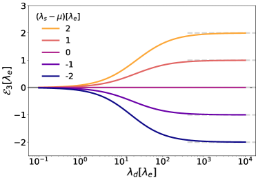
Figure 2: Unstable eigenvalue $\mathcal{E}_{3}$ (solid lines) as a function of doubling rate $\lambda_{d}$ for different values of $\lambda_{s}$ (color code) and $\mu=10\lambda_{e}$. The sign of $\mathcal{E}_{3}$ is the same of $\lambda_{s}-\mu$, and its value also stabilizes at $\lambda_{s}-\mu$ for very large values of $\lambda_{d}$ (dashed lines).

In the case of $\lambda_{s}=\mu$, it is possible to calculate the stationary value of of $\boldsymbol{\rho}(x,t\rightarrow\infty)$ as a function of the initial conditions $\boldsymbol{\rho}(x,0)$:

$$\rho_{+}(x,t\rightarrow\infty) =\frac{\lambda_{d}}{2(2\mu+\lambda_{d})}R(x,0)$$

$$\rho_{0}(x,t\rightarrow\infty) =\frac{\mu}{2\mu+\lambda_{d}}R(x,0)$$ (12)

$$\rho_{-}(x,t\rightarrow\infty) =\frac{\lambda_{d}}{2(2\mu+\lambda_{d})}R(x,0),$$

where $R(x,0)=2\rho_{0}(x,0)+\rho_{-}(x,0)+\rho_{+}(x,0)$. Since the exchange rate between right $\rho_{+}$ and left $\rho_{-}$ moving cells is symmetric, the amounts of left and right moving cells are the same in the stationary state ($\rho_{+}=\rho_{-}$, see also Figure 3). Furthermore, if $\lambda_{d}=2\mu=2\lambda_{s}$ all the three populations equilibrate to the same value, independently of the initial conditions. In the case of $\lambda_{s}>\mu$ it is always possible in the frame of the nonlinear growth model to find values of $\boldsymbol{\rho}_{c}$ for which the populations stabilize around the values given by Eq.(3.1). Figure 3 shows the linear and nonlinear model equations with different parameters and with the same stationary values.

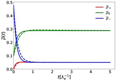
Figure 3: Space averages of right- $\overline{\rho}_{+}$, left-moving $\overline{\rho}_{-}$ and sedentary $\overline{\rho}_{0}$ cells as functions of time, both for the linear model (solid lines) with $\lambda_{s}=\mu$ and for the nonlinear model (dashed lines) with $\lambda_{s}=3\mu$. For both models $\lambda_{d}$ is set to be equal to $\lambda_{e}$, while $\mu=\lambda_{e}$ in the nonlinear model and $\mu=2.848\lambda_{e}$ in the linear one. As initial conditions we chose the constant values $\boldsymbol{\rho}(x,0)=(0,.1,0.479)$ for both models. For the nonlinear model we further set the carrying capacity $\boldsymbol{\rho}_{c}(x)=(1,1,1)$.

3.2 Density dynamics

We now set the running speeds $v_{\pm}$ and the diffusion constant $D$ to finite values, in order to study the evolution of spatial quantities of the system, such as the mean displacement MD $=\langle x-x_{0}\rangle$, the mean-squared displacement MSD $=\langle(x-x_{0})^{2}\rangle$ and all the higher order moments, where $x_{0}$ is the average position of the system at $t=0$. Here, the average $\langle(\cdot)\rangle$ is defined as $\int_{-\infty}^{\infty}(\cdot)P(x,t)\text{d}x$, where the total probability $P(x,t)$ is

$$P(x,t)\equiv\frac{1}{N(t)}(\rho_{+}(x,t)+\rho_{0}(x,t)+\rho_{-}(x,t)),$$ (13)

$N(t)\equiv N_{0}(t)+N_{+}(t)+N_{-}(t)$ is the total number of cells, $N_{\alpha}(t)=\int_{-\infty}^{\infty}\rho_{\alpha}(x,t)\text{d}x$ is the number of cells in phase $\alpha$ and $\alpha$ can be $(+,-,0)$.

In order to compute averages, we first solve the system by using a Fourier transform ($FT$):

$$\dot{\tilde{\boldsymbol{\rho}}}(k,t)=\left(-k^{2}\mathcal{D}-\text{i}k\mathcal{V}+\mathcal{M}\right)\tilde{\boldsymbol{\rho}}(k,t),$$ (14)

where $\tilde{\boldsymbol{\rho}}(k,t)=FT(\boldsymbol{\rho}(x,t))$ is the Fourier transform of $\boldsymbol{\rho}(x,t)$ and $k$ is the wave number conjugate to $x$. Similarly to the constant density case, the solution in Fourier space will be given by

$$\tilde{\boldsymbol{\rho}}(k,t)=\text{exp}\left[(-k^{2}\mathcal{D}-\text{i}k\mathcal{V}+\mathcal{M})t\right]\tilde{\boldsymbol{\rho}}(k,0).$$ (15)

One can use the solution of this equation to extract the intermediate scattering function (ISF)

$$\mathcal{F}(k,t)\equiv\tilde{P}(k,t)\tilde{P}(-k,0)N(t).$$ (16)

The ISF can be related to the different moments of the density kurzthaler_intermediate_2016 by differentiation:

$$\langle(x(t)-x_{0})^{n}\rangle=\left.\frac{\text{i}^{n}}{N(t)}\frac{\partial^{n}}{\partial k^{n}}\mathcal{F}(k,t)\right|_{k=0},$$ (17)

valid in one dimension (see Appendix).

We can also define an average for each cell population and the relative ISF:

$$\langle(\cdot)\rangle_{\alpha} \equiv \int_{-\infty}^{\infty}(\cdot)\frac{\rho_{\alpha}(x,t)}{N_{\alpha}(t)}\text{d}x,$$ (18)

$$\mathcal{F}_{\alpha}(k,t) \equiv \frac{\tilde{\rho}_{\alpha}(k,t)\tilde{\rho}_{\alpha}(-k,0)}{N_{\alpha}(0)}.$$ (19)

The expression corresponding to Eq.(17) is then given by

$$\langle(x(t)-x_{0})^{n}\rangle_{\alpha}=\left.\frac{\text{i}^{n}}{N_{\alpha}(t)}\frac{\partial^{n}}{\partial k^{n}}\mathcal{F}_{\alpha}(k,t)\right|_{k=0}.$$ (20)

First we will discuss the behavior of the whole distribution $P(x,t)$. For simplicity, we will consider the initial condition $\boldsymbol{\rho}(x,0)=(0,\delta(x),0)$ which is physically relevant, as it describes a cell initially settled in $x=0$ in the process of reproducing. We do not focus on the case of an initially mobile cell, as the short-time behaviours of both the MD and MSD turn out to be simply linear and the long-time behaviours are identical to that of the initially settled cell case. We further remark that our analysis does not assume the condition $\mu=\lambda_{s}$ for a stable population in the linear growth model.

3.2.1 Full distribution

When $v_{+}\neq v_{-}$, the MD is non-zero and we observe two different regimes: for short times it grows as $t^{2}$, while for long times it is proportional to $t$, as shown in Figure 4(a). The short-time expansion of the MD in fact yields

$$\langle x(t)-x_{0}\rangle = \lambda_{d}v_{d}t^{2}$$ (21)

$$-\frac{1}{3}\lambda_{d}v_{d}(2\mu+4\lambda_{d}+\lambda_{s})t^{3}$$

$$+\mathcal{O}\left(t^{4}\right),$$

where $v_{d}=(v_{+}-v_{-})/2$. The expression shows that both the transition rates and the running speeds have a role in determining this initial scaling regime. This can be interpreted as a composition of the doubling mechanism and the system acceleration given by cells suddenly starting to move. We can further define the typical crossover time $t_{c}^{(1)}$ as the ratio between absolute values of the coefficients of the $t^{2}$ and $t^{3}$ scalings, as this is the time at which the the $t^{2}$ order contribution becomes smaller than the following ones breoni_active_2020 ; breoni_active_2021 . This is a good estimate of the average time at which the dynamics is not dominated by the initial doubling anymore:

$$t_{c}^{(1)}=\frac{3}{2\mu+4\lambda_{d}+\lambda_{s}}.$$ (22)

The long-time expansion of the MD yields

$$\langle x(t)-x_{0}\rangle=\frac{4v_{d}\lambda_{d}\lambda_{s}}{\Lambda(\mu-\lambda_{d}+\lambda_{s}+\Lambda)}t+\mathcal{O}\left(t^{0}\right),$$ (23)

where $\Lambda$ is the same of Eq.(10).

As far as the MSD is concerned, in Figure 4(b) we still see a $t^{2}$ regime for short times, while the long-time behavior depends on the difference between $v_{-}$ and $v_{+}$. In the case they are the same, we will only see a diffusive long-time regime while otherwise this diffusive regime transitions into a ballistic one. The smaller the difference between the running speeds, the longer is the time to reach the ballistic regime. We further calculate the short-time expansion of the MSD:

$$\langle(x(t)-x_{0})^{2}\rangle = 2D\lambda_{d}t^{2}$$ (24)

$$-\frac{2}{3}\lambda_{d}\left(D(2\mu+4\lambda_{d}+\lambda_{s})-v_{a}^{2}\right)t^{3}$$

$$+\mathcal{O}\left(t^{4}\right),$$

where $v_{a}=\sqrt{(v_{+}^{2}+v_{-}^{2})/2}$. Again, we define a crossing time $t_{c}^{(2)}$ for the MSD as the ratio between the absolute values of the coefficients of the $t^{2}$ and $t^{3}$ scalings:

$$t_{c}^{(2)}=\frac{3D}{\left|D(2\mu+4\lambda_{d}+\lambda_{s})-v_{a}^{2}\right|}.$$ (25)

If we change the population rates we observe that the growth or decay in the number of cells does not influence qualitatively the scalings we just described for both the MD and MSD. The formula for the long-time expansion of the MSD and the relative crossing time $t_{l}^{(2)}$ between the long-time regimes $\propto t$ and $\propto t^{2}$ are quite involved, so we refrain from showing them here.
Finally, we study directly the full intermediate scattering function $\mathcal{F}(k,t)$ as it carries more information than the MSD and MD. In Figure 5 (a), that is in the case of equal velocities, we can see that the real part of $\mathcal{F}(k,t)$ that generates the MSD among all other even moments, decays rapidly for small length scales (i.e. large $k$) while it has three distinct regimes for large length scales. At first the function decays or grows, following the growth in the number of cells, then at time $t^{(2)}_{c}$ it plateaus for a time that grows larger as $k$ gets smaller, and finally decays completely. The plateau, starting after the transition of the cell to its moving stage at time $t^{(2)}_{c}$, is generated by the active cells going back to the settled stage and not moving anymore, while the final decay represents the long-time diffusive behavior that we have already seen in the MSD. In Figure 5 (b) we see how unequal velocities change the intermediate scattering function by introducing an oscillating behavior at long times. This is a signature of ballistic motion and of a non-vanishing imaginary part of $\mathcal{F}(k,t)$ that generates the odd moments like the MD.

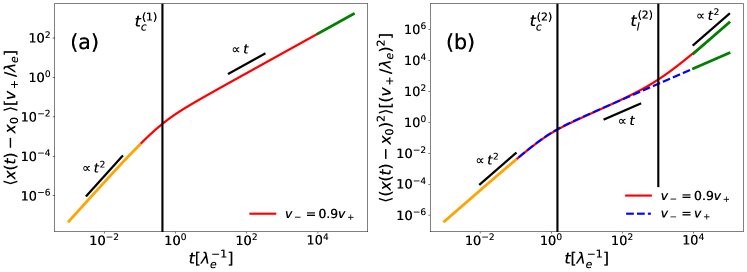
Figure 4: (a) Mean displacement (MD), (b) mean-squared displacement (MSD), respective crossing times $t_{c}^{(1)}$, $t_{c}^{(2)}$ and short- and long-time approximations for the initial conditions $\boldsymbol{\rho}(x,0)=(0,\delta(x),0)\lambda_{e}/v_{+}$, all rates equal to $\lambda_{e}$ and $D=0.2v_{+}^{2}/\lambda_{e}$. In (b) the solid red line shows unequal swim velocities ($v_{-}=0.9v_{+}$) and the dashed blue line equal swim speeds ($v_{-}=v_{+}$). The orange lines represent the short-time approximations, while the green lines are the long-time approximations.

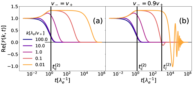
Figure 5: Real part of the intermediate scattering function $\mathcal{F}(k,t)$ for (a) equal swimming speeds and (b) unequal swimming speeds ($v_{-}=0.9v_{+}$) for the initial conditions $\boldsymbol{\rho}(x,0)=(0,\delta(x),0))\lambda_{e}/v_{+}$, all rates equal to $\lambda_{e}$ and $D=0.2v_{+}^{2}/\lambda_{e}$. The black lines represent the MSD short crossing time $t_{c}^{(2)}$ and, in the case of different speeds, long crossing time $t_{l}^{(2)}$.

3.2.2 Distribution of settled cells

The main feature of the MD and MSD of the settled cells is that they both show an initial $t^{3}$ regime, as shown in Figure 6. The short time expansion of the MD is given by

$$\langle x(t)-x_{0}\rangle_{0} = \frac{1}{3}\lambda_{s}\lambda_{d}v_{d}t^{3}$$ (26)

$$-\frac{1}{6}\lambda_{s}\lambda_{d}v_{d}(\mu-\lambda_{d}+\lambda_{s})t^{4}$$

$$+\mathcal{O}\left(t^{5}\right),$$

with the crossing time between the $t^{3}$ and $t^{4}$ regimes $t_{c,0}^{(1)}$ being:

$$t_{c,0}^{(1)}=\frac{2}{|\mu-\lambda_{d}+\lambda_{s}|}.$$ (27)

The MSD shows the initial $t^{3}$ regime as well:

$$\langle(x(t)-x_{0})^{2}\rangle_{0} = \frac{2}{3}D\lambda_{s}\lambda_{d}t^{3}$$ (28)

$$-\frac{1}{6}\lambda_{s}\lambda_{d}\left(2D(\mu-\lambda_{d}+\lambda_{s})-v_{a}^{2}\right)t^{4}$$

$$+\mathcal{O}\left(t^{5}\right).$$

with the crossing time $t_{c,0}^{(2)}$:

$$t_{c,0}^{(2)}=\frac{4D}{\left|2D(\mu-\lambda_{d}+\lambda_{s})-v_{a}^{2}\right|}.$$ (29)

The reason why we observe the $t^{3}$-behaviour for short times is the fact that the settled population can only change by doubling, moving and then settling, with each one of these processes being at least of order $t$. We also notice that for $D=0$ the MSD grows initially with $t^{4}$, as in this case the short time MSD for moving cells grows with $t^{2}$ and not $t$.
The long-time asymptotes for both MD and MSD of the settled particles are identical to those of the whole population.

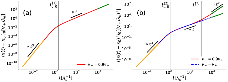
Figure 6: (a) Mean displacement (MD), (b) mean-square-displacement (MSD), respective crossing times $t_{c}^{(1)}$, $t_{c}^{(2)}$ and short- and long-time approximations for settled cells, with initial conditions $\boldsymbol{\rho}(x,0)=(0,\delta(x),0))\lambda_{e}/v_{+}$, all rates equal to $\lambda_{e}$ and $D=0.2v_{+}^{2}/\lambda_{e}$. In (b) the solid red line shows unequal swim velocities ($v_{-}=0.9v_{+}$) and the dashed blue line equal swim speeds ($v_{-}=v_{+}$). The orange lines represent the short-time approximations, while the green lines are the long-time approximations.

4 Interacting cells

4.1 Attraction to settled regions

We now discuss the case of interacting cells. Our model contains an effective attractive force that pushes the moving cells towards the regions where the density of settled cells is larger. This force is meant to represent how bacteria tend to assemble in resource-rich regions to reproduce or how they accumulate in order to form biofilms hall-stoodley_bacterial_2004 ; mazza_physics_2016 ; therefore the parameter $\kappa>0$ in Eq.(1). The interaction terms $\kappa\partial_{x}(\partial_{x}(\rho_{0})\rho_{\pm})$ render the equation nonlinear such that it is not analytically solvable. Instead we first perform a linear stability analysis around the homogeneous stationary solution to the linear system $\hat{\boldsymbol{\rho}}$ computed in Eq. (3.1) (see also Fig. 3) by adding a small perturbation $\delta\boldsymbol{\rho}(x,t)$ and neglecting the nonlinear terms in the perturbation $(\delta\boldsymbol{\rho}(x,t))^{2}$. We then arrive at the following system of equations for the perturbation:

$$\partial_{t}\delta\rho_{+}= -v_{+}\partial_{x}\delta\rho_{+}-\kappa\partial_{x}^{2}(\delta\rho_{0})\hat{\rho}_{+}+D\partial_{x}^{2}\delta\rho_{+}$$

$$-(\lambda_{s}+\lambda_{e}+\mu)\delta\rho_{+}+\lambda_{e}\delta\rho_{-}+\lambda_{d}\delta\rho_{0}$$

$$\partial_{t}\delta\rho_{0}= -\lambda_{d}\delta\rho_{0}+\lambda_{s}(\delta\rho_{+}+\delta\rho_{-})$$ (30)

$$\partial_{t}\delta\rho_{-}= v_{-}\partial_{x}\delta\rho_{-}-\kappa\partial_{x}^{2}(\delta\rho_{0})\hat{\rho}_{-}+D\partial_{x}^{2}\delta\rho_{-}$$

$$-(\lambda_{s}+\lambda_{e}+\mu)\delta\rho_{-}+\lambda_{e}\delta\rho_{+}+\lambda_{d}\delta\rho_{0},$$

where the stationary values for the density are symmetric, $\hat{\rho}_{+}=\hat{\rho}_{-}$. We apply both a Fourier transform in space and a Laplace transform in time to Eq. (30) and solve the resulting characteristic equation of the system. We obtain three different solutions for the eigenvalues of the system $s_{i}(k)$, of which only one, $s_{1}(k)$, can have a positive real part. In the following we focus on $s_{1}(k)$, since its positive real part introduces instabilities in the system.

First of all, for $k\rightarrow 0$, the value of $s_{1}(k)$ is one of the eigenvalues of the system matrix where the initial densities are constant, and more specifically the one that can be positive:

$$s_{1}(0)=\mathcal{E}_{3}\simeq\frac{\lambda_{d}(\lambda_{s}-\mu)}{\mu+\lambda_{d}+\lambda_{s}}.$$ (31)

This means that one of the conditions for the system to be stable is that the number of cells does not grow exponentially, which is expected.

The second limit we consider is $k\rightarrow\infty$. We have that

$$\lim_{k\rightarrow\infty}s_{1}(k)\rightarrow\frac{2\kappa\hat{\rho}_{+}\lambda_{s}}{D}-\lambda_{d}.$$ (32)

This second condition states that the diffusion constant contrasts directly the instabilities generated by a large settling rate and the attractive constant $\kappa$, as it disperses too large clusters of active cells, while a large doubling rate helps the stability by reducing the size of groups of settled cells. Knowing the limits of $s_{1}(k)$ in $k=0$ and $k=\infty$, i.e long- and short-range perturbations respectively, we are sure that the system will be unstable if the real part of either of them is larger than zero, giving us two stability conditions for the system:

$$\mu\geq\lambda_{s},$$

$$\lambda_{d}\geq\frac{2\kappa\hat{\rho}_{+}\lambda_{s}}{D}.$$ (33)

For $D=0$, $s_{1}(k)$ grows asymptotically like $k$, making the system always unstable. In Figure 7 we show the behavior of the eigenvalue Re$(s_{1}(k))$ for different values of $D$. Notice that for the set of parameters considered, if $D=2v_{+}^{2}/\lambda_{e}$ the stability conditions are only narrowly fulfilled, but the real part of $s_{1}$ stays negative for all the values of $k$. Lastly, when the cell running speeds are not isotropic, the imaginary part of $s_{1}$ can be non-zero, meaning that there can be stable periodicity in the system.

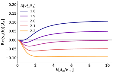
Figure 7: Eigenvalue $s_{1}(k)$ as a function of wavenumber $k$ for different values of $D$, where all rates are equal to $\lambda_{e}$, $v_{-}=v_{+}$ and $\kappa=\lambda_{e}^{-1}$.

While the real part of the other two solutions $s_{2}$ and $s_{3}$ is always negative, their imaginary part is non-zero for large values of $k$. More specifically, for large $k$ and finite $D$ their imaginary part is proportional to $k$, while the real part goes with $-Dk^{2}$. A finite imaginary part indicates oscillations in the system, although the negative real part means that these oscillations are only transient. Signatures of these oscillations can also be seen in our numerical solutions (see the next Section).

4.2 Repulsion among settled cells

We now include a self-repulsive potential for the cells that do not move, given by $\kappa_{0}>0$ in the matrix $\mathcal{U}$ in Eq. 1. This repulsion models the need for settled bacteria to not overcrowd any particular region and deplete its resources while reproducing. What is particularly interesting about having both an attractive and a repulsive part in the potential is that the interplay of these two opposing effects can lead to structures forming in the system, as we will show now. If we repeat the analysis described in the last subsection including $\kappa_{0}>0$, we find that the limits of $s_{1}(k)$ are

$$s_{1}(0) = \mathcal{E}_{3}$$

$$s_{1}(k\rightarrow\infty) = -\kappa_{0}\hat{\rho_{0}}k^{2}+\mathcal{O}(k).$$ (34)

The main difference with Eqs.(31),(32) is that $s_{1}$ will always be negative for a sufficiently large value of $k$. This means that if we choose parameters for which $s_{1}$ can be positive, its largest root $k_{r}$ will indicate the smallest allowed instability of the system, with size $l=2\pi/k_{r}$. We consequently expect instabilities to form for systems of size $L$ larger than $l$. As an example of this we numerically calculated the values of $k_{r}$ for different values of the running speeds $v_{+}$ and $v_{-}$, quantifying their occurrence using two non-dimensional parameters, the maximum speed $v_{m}$ and the reduced difference speed $v_{r}$ defined by

$$v_{m}\equiv\frac{\text{max}(v_{+},v_{-})}{\sqrt{D\lambda_{e}}}\qquad v_{r}\equiv\frac{v_{+}-v_{-}}{v_{+}+v_{-}}.$$ (35)

We chose specifically to vary the running speeds as they can easily tune the asymmetry of the system, leading to interesting instabilities. In Figure 8 we can see $k_{r}$ as a function of $v_{r}$ and $v_{m}$, written in units of $k_{0}=2\pi/L$. We expect the system to develop instabilities for values of $k_{r}>k_{0}$, so we fitted the separatrix $k_{r}=k_{0}$ to a second-order polynomial, $v_{m}^{f}(v_{r})$:

$$v_{m}^{f}=2.76\pm 0.01+(2.73\pm 0.03)v_{r}-(1.14\pm 0.04)v_{r}^{2}.$$ (36)

This particular fit was determined using the linear growth model for the parameter values indicated in the caption to Figure 8.

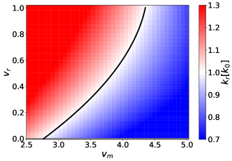
Figure 8: Largest root of $s_{1}(k)$, $k_{r}$, as function of $v_{r}$ and $v_{m}$. As parameters we chose $\lambda_{s}=\lambda_{d}=\mu=0.1\lambda_{e}$, $\kappa=0.2\lambda_{e}^{-1}$, $\kappa_{0}=0.05\lambda_{e}^{-1}$ and $D=0.001L^{2}\lambda_{e}$. In blue we see the parameters for which the system is not large enough to enable instabilities, while in black we have the second order polynomial that fits the $k_{r}=k_{0}$ curve.

In order to study the emergence of such instabilities in detail, we further implemented a numerical solver for both Eqs.(1) and (6), using an explicit fourth-order Runge-Kutta algorithm press_numerical_2007 for the time integration and a finite difference scheme in space. We performed calculations both with the linear and the nonlinear growth model, setting respectively $\lambda_{s}=\mu$ and $\lambda_{s}\geq\mu$. We use a finite box of length $L$ with periodic boundary conditions. Setting the time step to $\Delta t=10^{-4}\lambda_{e}^{-1}$ we calculated $\sim 10^{6}$ steps to ensure that the system settles into a steady state. Our calculations are initialized using the steady-state solutions of the linear system (Eqs. (3.1)), to which we add small fluctuations given by Gaussian noise. We find that our system develops wave-like structures, which are static for $v_{+}=v_{-}$ and become traveling waves when $v_{+}\neq v_{-}$ - see Figure 9 for the linear growth case and Figure 11 for the nonlinear case. Testing different initial conditions, e.g. choosing $\rho_{0}(x)$ as a narrow Gaussian peak that approximates an initially settled single cell, we also observed that these wave-like structures always form, even if the specific shape of the wave can be affected. In our analysis we preferred to use the steady-state solution of Eqs.(3.1) as initial condition, as it makes comparison with the theoretical results of Figure 8 more straightforward. Intuitively, the attractive term $\kappa$ leads to the formation of peaks, induced by the instability in Eq.(33). These peaks are then stabilized by the repulsive term $\kappa_{0}$. The asymmetry of the running speeds makes the peaks move.

Migrating bands of bacteria have indeed been observed experimentally adler_chemotaxis_1966 ; adler_effect_1966 ; adler_chemoreceptors_1969 ; berleman_rippling_2006 ; stricker_hybrid_2020 ; liu_viscoelastic_2021 and have also been modeled theoretically cremer_chemotaxis_2019 ; narla_traveling-wave_2021 ; caprini_collective_2021 , always considering only one species of cells. A particularly surprising feature of our model is that in this final stationary state all three distributions evolve in the same direction at the same speed, independently of the intrinsic running speed of the cells.

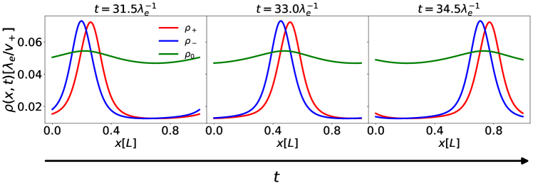
Figure 9: Density of left $\rho_{-}$, right $\rho_{+}$ and sedentary $\rho_{0}$ cells as functions of space at different times (increasing from (a) to (c)). We set here $\lambda_{s}=\lambda_{d}=\mu=.1\lambda_{e}$, $\kappa=.2\lambda_{e}^{-1}$, $\kappa_{0}=.05\lambda_{e}^{-1}$, $v_{+}=2v_{-}=.1L\lambda_{e}$ and $D=0.001L^{2}\lambda_{e}$.

We replicated the diagram of Figure 8 with numerical integration of the model equation, and the resulting non-equilibrium state diagram is shown in Figure 10. We find a clear transition from a stable system (shown in blue), where all species are constant in space, to the appearance of wave-like structures (shown in red to yellow). The gradient visualizes the change in stationary speed of the waves $v_{s}$, defined as the speed of the waves in the stationary state divided by $\sqrt{D\lambda_{e}}$, and is hence non-dimensional. This quantity is almost vanishing near the transition, and grows the further away we move from it. The formation of these waves is typical of systems with a large difference between $v_{+}$ and $v_{-}$ or rather small absolute speeds. We fitted the separatrix to a second order polynomial $v_{m}^{f}(v_{r})$ and obtained

$$v_{m}^{f}=2.78\pm 0.01+(2.56\pm 0.03)v_{r}-(0.88\pm 0.03)v_{r}^{2}.$$ (37)

We find that our numerical calculations and theory are in very good qualitative agreement.

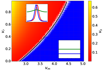
Figure 10: State diagram of the system as a function of $v_{r}$ and $v_{m}$. As parameters we chose $\lambda_{s}=\lambda_{d}=\mu=0.1\lambda_{e}$, $\kappa=0.2\lambda_{e}^{-1}$, $\kappa_{0}=0.05\lambda_{e}^{-1}$ and $D=0.001L^{2}\lambda_{e}$. In blue we see the parameters for which the system is stably constant, while in red to yellow we see the parameters for which the system generates traveling wave structures. Examples of both long-time behaviors are shown in their respective area. The gradient shows the stationary velocity of the waves $v_{s}$, while in black we have the second order polynomial that fits the transition curve $v_{m}^{f}$.

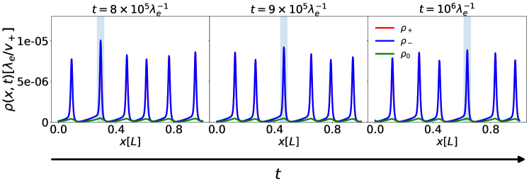
Figure 11: Nonlinear growth model, density of left $\rho_{-}$, right $\rho_{+}$ and sedentary $\rho_{0}$ cells as functions of space at different times (increasing from (a) to (c)). Because of the large value of $\lambda_{e}$ compared to the other rate parameters, the right-moving and left-moving populations have almost the same shape, making the red line disappear under the blue line. The shaded areas indicate the largest peak, and how it moves in time towards the right. We chose as parameters the values typical of CC shown in Table 1. For the interaction potentials, for which no experimental estimates can be made at present, we chose $\kappa=\kappa_{0}=10\lambda_{e}^{-1}$, while for the carrying capacity of the system we set $\boldsymbol{\rho}_{c}(x,t)=(0.04,0.04,0.04)\lambda_{e}/v_{+}$.

4.3 Application to Caulobacter crescentus

Table 1 gives an idea of the experimentally measured values for CC which have been extracted from recent papers on its swimming behaviour li_low_2006 ; lin_single-gene_2010 ; liu_helical_2014 ; lele_flagellar_2016 . It is noteworthy to comment on the running speeds $v_{+},v_{-}$. While the torque generated by the flagellar motor differs significantly during forward and backward motion, the resulting velocities are not dramatically different (and, in fact, experimentally hard to measure) lele_flagellar_2016 .

run-and-tumbling rate; $s^{-1}$	$\lambda_{e}$	$10^{-1}$
settling rate; $s^{-1}$	$\lambda_{s}$	$10^{-5}$
doubling rate; $s^{-1}$	$\lambda_{d}$	$10^{-4}$
decay rate; $s^{-1}$	$\mu$	$10^{-6}$
running speed right; $m/s$	$v_{+}$	$4\cdot 10^{-5}$
running speed left; $m/s$	$v_{-}$	$3.5\cdot 10^{-5}$
diffusion coefficient; $m^{2}/s$	$D$	$2\cdot 10^{-9}$

Table 1: Values of the parameters for Caulobacter crescentus taken from li_low_2006 ; lin_single-gene_2010 ; liu_helical_2014 ; lele_flagellar_2016 .

We have performed calculations with the parameters of Table 1 for different values of $\kappa$ and $\kappa_{0}$ which are undetermined from experiments. Since for Caulobacter $\mu<\lambda_{s}$, we have included the saturating nonlinearity for the growth in the model. The results show that the waves still form provided the ratio $\kappa/\kappa_{0}$ is large enough (Figure 11).

5 Conclusions and outlook

In this work we proposed and studied a 1D 3-state model motivated by the cell cycle progression of the bacterium Caulobacter crescentus, including both its run and tumble motion and its reproductive behavior. We first analyzed the free cell space-independent case and calculate the parameter regimes for which the number of cells grows or declines. Adding the spatial dependence we subsequently determined dynamical quantities of the system such as the mean displacement, the mean-squared displacement and the intermediate scattering function. We found a surprising super-ballistic behavior of the MSD at short times with a $t^{3}$ scaling which stems from the interplay of cells doubling and cells starting to swim.

Subsequently, we included attractive and repulsive interactions between cells into our model, representing their tendency to swim towards regions in which cells are settled and to avoid overcrowding. We determined the stability conditions and, using numerical methods, we studied the fully nonlinear system in which we identify traveling waves of cells. Their occurrence is quantified in a non-equilibrium state diagram.

Our model lends itself to further extensions in several ways. E.g., one could account for complex nutrient landscapes and for a more detailed description of the cell cycle, which is well-studied from various aspects biondi_cell_2022 ; another possible system for application are Chlamydomonas reinhartii cells harris_chlamydomonas_2009 . The cell cycle can be included in cell-resolved simulations such as performed recently in you_geometry_2018 ; schwarzendahl_notitle_2022 . Another direction could be a two-dimensional field description that includes the nematic ordering of cells such as in dellarciprete_growing_2018 . In a higher-dimensional model it would also be interesting to see what the effect of different swimming strategies such as run and tumble, run-reverse or run-reverse-flick grognot_more_2021 is. Finally, an exploration of the fully nonlinear model - nonlinear diffusive interactions as well as nonlinear growth - including a full higher-dimensional tumbling behaviour for a multi-species system would be an interesting problem in the context of biofilm growth.

Appendix

Relation between intermediate scattering function and momenta of the density in 1D

We show here the calculation that justifies Eq.(17) in one dimension in the case where the initial conditions for the cell density are $\boldsymbol{\rho}(x,t=0)=(0,N(0)\delta(x),0)$. First, we write the definition for the moments $\langle(x(t)-x_{0})^{n}\rangle=\langle x^{n}(t)\rangle$:

$$\langle x^{n}(t)\rangle=\int_{-\infty}^{\infty}\text{d}x\,x^{n}P(x,t),$$ (38)

where $P(x,t)$ is the probability density of the position. We then apply a Fourier transform and its inverse in the integral

$$\langle x^{n}(t)\rangle=\frac{1}{2\pi}\int_{-\infty}^{\infty}\text{d}x\int_{-\infty}^{\infty}\text{d}k\,\text{e}^{ikx}\left(\text{i}^{n}\frac{\partial^{n}\tilde{P}(k,t)}{\partial k^{n}}\right),$$ (39)

where $\tilde{P}(k,t)$ is the Fourier Transform of $P(x,t)$. Finally, we exchange the order of integration to get

$$\langle x^{n}(t)\rangle = \frac{1}{2\pi}\int_{-\infty}^{\infty}\text{d}k\,2\pi\delta(k)\left(\text{i}^{n}\frac{\partial^{n}\tilde{P}(k,t)}{\partial k^{n}}\right)$$ (40)

$$= \left.\text{i}^{n}\frac{\partial^{n}\tilde{P}(k,t)}{\partial k^{n}}\right|_{k=0}.$$

Knowing that for the initial conditions that we have chosen $\tilde{\boldsymbol{\rho}}(-k,0)=(0,N(0),0)$, we have

$$\mathcal{F}(k,t)\equiv\tilde{P}(k,t)\tilde{P}(-k,0)N(t)=\tilde{P}(k,t)N(t),$$ (41)

and hence

$$\langle x^{n}(t)\rangle=\left.\text{i}^{n}\frac{\partial^{n}\tilde{P}(k,t)}{\partial k^{n}}\right|_{k=0}=\left.\frac{\text{i}^{n}}{N(t)}\frac{\partial^{n}\mathcal{F}(k,t)}{\partial k^{n}}\right|_{k=0}.$$ (42)

Author contribution statement

HL and RB directed the project. DB performed analytic calculations and numerical simulations. All authors discussed the results and wrote the manuscript.

Data Availability Statement

The datasets generated during and/or analysed during the current study are available from the corresponding author on reasonable request.

References

- (1) Berg H C (ed) 2004 E. coli in Motion Biological and Medical Physics, Biomedical Engineering (New York, NY: Springer) ISBN 978-0-387-00888-2 978-0-387-21638-6
- (2) Berg H C 2018 Random Walks in Biology: New and Expanded Edition (Princeton University Press) ISBN 978-1-4008-2002-3
- (3) Elgeti J, Winkler R G and Gompper G 2015 Reports on Progress in Physics 78 056601
- (4) Polin M, Tuval I, Drescher K, Gollub J P and Goldstein R E 2009 Science 325 487–490
- (5) Detcheverry F 2017 Physical Review E 96 012415
- (6) Fier G, Hansmann D and C Buceta R 2018 Soft Matter 14 3945–3954
- (7) Bertrand T, Illien P, Bénichou O and Voituriez R 2018 New Journal of Physics 20 113045
- (8) Maes C, Meerts K and Struyve W 2022 Physica A: Statistical Mechanics and its Applications 127323
- (9) Angelani L 2017 Journal of Physics A: Mathematical and Theoretical 50 325601
- (10) Angelani L and Garra R 2019 Physical Review E 100 052147
- (11) Dhar A, Kundu A, Majumdar S N, Sabhapandit S and Schehr G 2019 Physical Review E 99 032132
- (12) Singh P and Kundu A 2021 Physical Review E 103 042119
- (13) Monthus C 2021 Journal of Statistical Mechanics: Theory and Experiment 2021 083212
- (14) Frydel D 2021 Journal of Statistical Mechanics: Theory and Experiment 2021 083220
- (15) Dandekar R, Chakraborti S and Rajesh R 2020 Physical Review E 102 062111
- (16) Singh P, Sabhapandit S and Kundu A 2020 Journal of Statistical Mechanics: Theory and Experiment 2020 083207
- (17) Le Doussal P, Majumdar S N and Schehr G 2021 Physical Review E 104 044103
- (18) Barriuso Gutiérrez C M, Vanhille-Campos C, Alarcón F, Pagonabarraga I, Brito R and Valeriani C 2021 Soft Matter 17 10479–10491
- (19) Mori F, Gradenigo G and Majumdar S N 2021 Journal of Statistical Mechanics: Theory and Experiment 2021 103208
- (20) Frydel D 2022 Physical Review E 105 034113
- (21) Garcia-Millan R and Pruessner G 2021 Journal of Statistical Mechanics: Theory and Experiment 2021 063203
- (22) Zhang Z and Pruessner G 2022 Journal of Physics A: Mathematical and Theoretical 55 045204
- (23) Basu U, Majumdar S N, Rosso A, Sabhapandit S and Schehr G 2020 Journal of Physics A: Mathematical and Theoretical 53 09LT01
- (24) Grange P and Yao X 2021 Journal of Physics A: Mathematical and Theoretical 54 325007
- (25) Frydel D 2022 Physics of Fluids 34 027111
- (26) Shebelut C W, Guberman J M, van Teeffelen S, Yakhnina A A and Gitai Z 2010 Proceedings of the National Academy of Sciences 107 14194–14198
- (27) Biondi E (ed) 2022 Cell Cycle Regulation and Development in Alphaproteobacteria (Cham: Springer International Publishing) ISBN 978-3-030-90620-7 978-3-030-90621-4
- (28) Harris E, Stern D and Witman G 2009 The Chlamydomonas Sourcebook 1
- (29) Narla A V, Cremer J and Hwa T 2021 Proceedings of the National Academy of Sciences 118 e2105138118
- (30) Grognot M and Taute K M 2021 Current Opinion in Microbiology 61 73–81
- (31) Son K, Guasto J S and Stocker R 2013 Nature Physics 9 494–498
- (32) Kurzthaler C, Leitmann S and Franosch T 2016 Scientific Reports 6 36702
- (33) Breoni D, Schmiedeberg M and Löwen H 2020 Physical Review E 102 062604
- (34) Breoni D, Löwen H and Blossey R 2021 Physical Review E 103 052602
- (35) Hall-Stoodley L, Costerton J W and Stoodley P 2004 Nature Reviews Microbiology 2 95–108
- (36) Mazza M G 2016 Journal of Physics D: Applied Physics 49 203001
- (37) Press W H, Teukolsky S A, Vetterling W T and Flannery B P 2007 Numerical Recipes 3rd Edition: The Art of Scientific Computing (Cambridge University Press) ISBN 978-0-521-88068-8
- (38) Adler J 1966 Science (New York, N.Y.) 153 708–716
- (39) Adler J 1966 Journal of Bacteriology 92 121–129
- (40) Adler J 1969 Science 166 1588–1597
- (41) Berleman J E, Chumley T, Cheung P and Kirby J R 2006 Journal of Bacteriology 188 5888–5895
- (42) Stricker L, Guido I, Breithaupt T, Mazza M G and Vollmer J 2020 Journal of The Royal Society Interface 17 20200559
- (43) Liu S, Shankar S, Marchetti M C and Wu Y 2021 Nature 590 80–84
- (44) Cremer J, Honda T, Tang Y, Wong-Ng J, Vergassola M and Hwa T 2019 Nature 575 658–663
- (45) Caprini L, Maggi C and Marini Bettolo Marconi U 2021 The Journal of Chemical Physics 154 244901
- (46) Li G and Tang J X 2006 Biophysical Journal 91 2726–2734
- (47) Lin Y, Crosson S and Scherer N F 2010 Molecular Systems Biology 6 445
- (48) Liu B, Gulino M, Morse M, Tang J X, Powers T R and Breuer K S 2014 Proceedings of the National Academy of Sciences 111 11252–11256
- (49) Lele P P, Roland T, Shrivastava A, Chen Y and Berg H C 2016 Nature Physics 12 175–178
- (50) You Z, Pearce D J, Sengupta A and Giomi L 2018 Physical Review X 8 031065
- (51) Schwarzendahl F J and Beller D A 2022 arXiv:2205.05185 [cond-mat, q-bio]
- (52) Dell’Arciprete D, Blow M L, Brown A T, Farrell F D C, Lintuvuori J S, McVey A F, Marenduzzo D and Poon W C K 2018 Nature Communications 9 4190