Data-driven dynamic treatment planning for chronic diseases

Data-driven dynamic treatment planning for chronic diseases

Christof Naumzik ETH Zurich, Weinbergstr. 56/58, 8092 Zurich, Switzerland, cnaumzik@ethz.ch, Stefan Feuerriegel (corresponding author) LMU Munich, Geschwister-Scholl-Platz 1, 80539 Munich, Germany, feuerriegel@lmu.de, Anne Molgaard Nielsen Department of Sports Science and Clinical Biomechanics, University of Southern Denmark, Denmark, amnielsen@health.sdu.dk,

In order to deliver effective care, health management must consider the distinctive trajectories of chronic diseases. These diseases recurrently undergo acute, unstable, and stable phases, each of which requires a different treatment regimen. However, the correct identification of trajectory phases, and thus treatment regimens, is challenging. In this paper, we propose a data-driven, dynamic approach for identifying trajectory phases of chronic diseases and thus suggesting treatment regimens. Specifically, we develop a novel variable-duration copula hidden Markov model (VDC-HMMX). In our VDC-HMMX, the trajectory is modeled as a series of latent states with acute, stable, and unstable phases, which are eventually recovered. We demonstrate the effectiveness of our VDC-HMMX model on the basis of a longitudinal study with 928 patients suffering from low back pain. A myopic classifier identifies correct treatment regimens with a balanced accuracy of slightly above 70%. In comparison, our VDC-HMMX model is correct with a balanced accuracy of 83.65%. This thus highlights the value of longitudinal monitoring for chronic disease management.

machine learning; treatment regimen; copula; Bayesian modeling; hidden Markov model

1 Introduction

Chronic diseases, such as depression, arthritis, cancer, diabetes, and non-specific low back pain, represent a considerable burden upon individuals and society. In the US alone, chronic diseases affect the quality of life of about 40 million individuals, nearly one third of the adult population (Blackwell et al. 2014). Owing to this prevalence, there is an urgent need for better chronic disease management. In particular, over- and under-treatment are critical, as these lead to suboptimal care (Trasta 2018).

Chronic disease management must be carefully adapted to the distinctive characteristics of chronic diseases. Chronic diseases are health conditions that are long-lasting or persistent (Bernell and Howard 2016). Furthermore, chronic diseases undergo different – and potentially recurrent – trajectory phases comprising acute, unstable, and stable periods (Corbin and Strauss 1991, Corbin 1998). In each of these trajectory phases, a chronic disease is characterized by different disease dynamics. It also demands different forms of care and thus requires tailored treatment regimens. If the trajectory phase changes, the treatment regimen must be updated accordingly. This has been formalized in the so-called chronic illness trajectory framework (Corbin and Strauss 1988, 1991).

Applying the above trajectory framework in practice is challenging. Despite this guideline being regarded as best practice (Larsen 2017), healthcare practitioners often adapt care to symptoms rather than the underlying trajectory (Snyderman 2012). The primary reason is that the identification of trajectory phases is non-trivial (Burton 2000). For one thing, trajectory phases and symptoms are only stochastically related. For instance, there might be a temporary change in symptoms, while the underlying trajectory phase remains unaffected (or vice versa). Hence, drawing inferences from symptoms rather than trajectory phases is sub-optimal (Corbin and Strauss 1988, 1991). This is shown on the basis of example health trajectories in Figure 1. Moreover, the course of symptoms is highly variable. Some variation in symptoms is thus stochastic in nature and should quickly revert to its original condition. Hence, it is often difficult to identify the onset of a new trajectory phase and thus when a new treatment regimen should be applied.

Notes: The plot shows the disease progression of three sample patients. The trajectory phases were annotated by medical experts and are shown in color, namely an acute trajectory phase in red, unstable in yellow, and stable in green. Left: The patient exhibits a quick recovery from a temporary relapse. Center: The patient has a temporary absence of symptoms, and yet a treatment regimen for an unstable trajectory phase would be preferable overall. Right: The patient experiences a sudden pain episode. By focusing on symptoms, a health professional might be inclined to recommend an acute treatment regimen (e. g., strong medicine with potential side-effects). Yet the symptoms would revert quickly and, hence, a stable treatment regimen (e. g., pain self-management) appears desirable. In all three examples, the trajectory phase is a better indicator of the true progression of the disease and, therefore, the guidelines from the trajectory framework (Corbin and Strauss 1991) advise basing treatment decisions on the trajectory phase (rather than on symptoms). Note that the above examples draw upon the complete course and thus benefit from post-hoc knowledge, whereas, in practice, the course would only be known partially. Hence, identifying a suitable treatment regimen in such a dynamic setting is challenging. Figure 1: Example Health Trajectories for Low Back Pain.

This work develops a data-driven approach to dynamic treatment planning for chronic diseases. For this purpose, we formed an interdisciplinary team with health researchers and designed our data-driven approach according to the trajectory framework: it dynamically determines the (latent) trajectory phase and, based on it, suggests an acute, unstable, or stable treatment regimen. Formally, we develop a novel variable-duration copula hidden Markov model (VDC-HMMX). In our VDC-HMMX, the health trajectory forms a a sequence of latent states (acute, stable, unstable), for which symptoms represent noisy realizations. Our VDC-HMMX then recovers the latent trajectory phases, which then prescribe the treatment regimens.

Thereby, our model extends the naïve HMM (MacDonald and Zucchini 1997, Rabiner 1989) in three ways: (1) a variable duration component, (2) a copula structure for multivariate emissions, and (3) heterogeneity in the transition. The latter includes risk variables that describe the between-patient heterogeneity. Previously, several works have used either variable-duration HMMs (e. g., Barbu and Limnios 2008, Chiappa 2014, Kundu et al. 1998, Limnios and Barbu 2008, Murphy 2002, Naumzik et al. 2021, Yu 2010) or copula HMMs (e. g., Brunel and Pieczynski 2005, Brunel et al. 2010, Härdle et al. 2015, Martino et al. 2018, Ötting et al. 2021). Both variable-duration HMM and copula HMM are later part of our baselines and outperformed by our proposed VDC-HMMX. However, to the best of our knowledge, no work has hitherto developed a HMM accommodating (1)–(3), thus making ours the first variable-duration copula HMM.

The effectiveness of our HMM is demonstrated based on a longitudinal study of almost $1,000$ patients suffering from recurrent low back pain. This disease is responsible for the greatest number of years spent with disability globally (GBD 2017). Based on a dynamic evaluation framework, we obtain the following finding. A myopic classifier (reflecting current practice) identifies the correct treatment regimen with a balanced accuracy of slightly above $70\text{\,}\mathrm{\char 37\relax}$, whereas the proposed HMM achieves a balanced accuracy of $83.65\text{\,}\mathrm{\char 37\relax}$. Our proposed HMM further outperforms a naïve HMM as well as a sequential neural network (long short-term memory).

Our work has direct implications for health management. First, health professionals should be careful if treatment decisions are based purely on symptoms: symptoms merely represent noisy realizations of the underlying health trajectory and thus prompt ineffective treatment regimens. Rather, the decision-making of health professionals should be aligned with the underlying trajectory phase. This latter approach provides a means by which over- and under-treatment could be alleviated. Second, health management could benefit from further personalization with regard to individual health trajectories. Third, our work encourages health professionals in chronic disease management to more widely utilize longitudinal health monitoring.

This paper is organized as follows. Section 2 reviews the trajectory framework as state-of-the-art practice in chronic disease management. Section 3 develops our novel variable-duration copula HMM. Section 4 presents our longitudinal study of low back pain. We then first select our preferred HMM specification (Section 5) and then benchmark it against baselines to demonstrate the effectiveness of our HMM for dynamically identifying treatment regimens (Section 6). Finally, Section 7 discusses implications for personalized chronic disease management. Section 8 concludes.

2 Background

2.1 Managing the Trajectory of Chronic Diseases

Managing chronic diseases aims at stabilizing the underlying course (Henly 2017). To this end, chronic disease management “does not necessarily mean altering the direction of the course” (Corbin and Strauss 1991), as this is usually not possible (Larsen 2017). Rather, chronic disease management aims at maintaining the current trajectory phase, as detailed in the following.

In chronic care, health management must adapt to the protracted, variable, and often recurrent course of chronic diseases (Bernell and Howard 2016). This has been formalized in the so-called trajectory framework (Corbin and Strauss 1991). Combining 30 years of health management research, this comprehensive framework facilitates the task of managing the course of chronic diseases. The framework was later extended to incorporate additional areas of medical practice, such as nursing (Corbin 1998), and today it has found widespread adoption in medical practice (Henly 2017, Larsen 2017, NHS Foundation Trust 2015).

The central concept in the trajectory framework is the so-called trajectory (Corbin and Strauss 1988, 1991), according to which a chronic disease undergoes different phases. These are listed in Table 1 as follows: (1) an acute phase represents the most critical situation, often with a need for immediate treatment to control symptoms, (2) an unstable phase entails a lack of full control over symptoms, and (3) a stable phase is one in which symptoms are controlled. These trajectory phases (acute, unstable, stable) are managed by care providers and thus fall within the scope of this paper. Additional trajectory phases (i. e., pretrajectory, trajectory onset, crisis) refer to the time before diagnosis, while others are relevant for palliative care (i. e., downward phase and decease, which describe a potential death). Previous research has repeatedly validated the trajectory framework for a variety of chronic diseases. Examples include, for instance, stroke rehabilitation (Burton 2000), HIV/AIDS (Corless and Nicholas 2000), epilepsy (Jacoby and Baker 2008), and cancer (Klimmek and Wenzel 2012).

Table 1: Trajectory Phases of Chronic Diseases (Corbin and Strauss 1991).

Trajectory phase	Description
Acute	Severe complications; the aim is stabilizing the condition through (ambulant) hospitalization
Unstable	Course of disease and symptoms not fully controlled by regimen; continuing care but no further hospitalization
Stable	Course of disease and symptoms are controlled by treatment regimen; no need for hospitalization, but self-management practices are often introduced
Note: Additional trajectory phases apply to the time before diagnosis and to palliative care (beyond the scope of this paper).

For chronic disease management, the trajectory framework has important implications: the trajectory phases refer to different disease dynamics and thus demand different forms of care (Larsen 2017). Accordingly, patients in acute, unstable, and stable phases should essentially be treated as different cohorts. Hence, the decision-making problem for health professionals is to manage the trajectory phase by choosing a treatment regimen that is “specific to the illness phasing” (Corbin and Strauss 1991). Put differently, if treatment regimen and trajectory do not match, the treatment is ineffective in managing the current disease dynamics, and thus represents over- or under-treatment (e. g., Kazemian et al. 2019). If the underlying trajectory phase changes, the treatment regimen must be adjusted accordingly.

When operationalizing the trajectory framework in practice, health professionals usually follow a two-stage approach (Larsen 2017): First, the patient’s symptoms are examined in order to identify the current trajectory phase. By knowing the current phase, healthcare professionals can adapt the treatment plan accordingly, that is, which treatment regimen (acute, unstable, stable) to choose and when to update the treatment regimen. Thereby, the trajectory framework ensures that the underlying disease dynamics (rather than merely symptoms) are treated. In a second stage, the design of the treatment regimen is chosen, e. g., among dimensions of the treatment regimen such as the type of medication and its dosage (cf. the next section for details). The design is a control task with the objective of maintaining the patient’s present status of symptoms. In contrast, deciding upon a trajectory phase, and thus a corresponding treatment regimen, represents an identification task. That is, the course of the symptoms is interpreted in order to determine the trajectory phase (Corbin and Strauss 1991).

Applying the trajectory framework in practice is subject to challenges. First, the trajectory phases are usually recurrent and long-lasting, that is, spanning weeks or sometimes even months. Hence, close monitoring is needed, so that the treatment regimens can be adjusted dynamically. Second, it is left open how practitioners in healthcare and nursing can actually infer the current trajectory phase (Corbin and Strauss 1991). Even though the past course of symptoms should be analyzed, clinical practice often lacks full information of this sort due to a lack of longitudinal monitoring. Third, trajectory phases and symptoms are only stochastically related. Within each phase, there may be temporary periods in which the symptoms can vary (i. e., temporary reversal or worsening of symptoms), although the underlying trajectory phase remains unchanged (Corbin and Strauss 1991). Hence, this represents a source of human error (e. g., Burton 2000), as the correct trajectory phases can often only be identified post-hoc.

2.2 Decision Support for Chronic Disease Management

In order to aid chronic disease management, prior literature has developed decision support to optimize treatment planning. This is summarized in the following.

Risk scoring is supposed to foster informed decision-making and thus helps both patients and health professionals by forecasting the future course of a disease, such as expected health outcomes (e. g., Bertsimas et al. 2017, Lin et al. 2017, Mueller-Peltzer et al. 2020, Fu et al. 2012) or readmission risk (e. g., Ayabakan et al. 2016, Bardhan et al. 2015). Some works even derive explicit target levels for certain risk factors (Helm et al. 2015, Kazemian et al. 2019). The pathways of chronic diseases are described based on models that can capture their long-term and recurrent dynamics. Hence, common choices are simple Markov chains or semi-Markov models (e. g., Chou et al. 2017, Srikanth 2015). However, these models assume the trajectory phases to be known a priori, whereas our objective is to identify them. Similarly, there have been a few works that accommodate hidden states, yet with clear differences from our work: These approaches operate on diagnosis codes (Alaa and van der Schaar 2018, Liu et al. 2015, Wang et al. 2014) or hospital readmissions (Ayabakan et al. 2016, Martino et al. 2018), but not symptoms. Furthermore, their purpose is predicting future risk, whereas we recover latent trajectory phases. As we shall see later, our objective requires a tailored modeling approach.

Various approaches have been developed that help in determining the design of a predefined treatment regimen. This involves, for instance, the type of medication (e. g., Bertsimas et al. 2017, Zargoush et al. 2018) and the corresponding dosage (e. g., Ibrahim et al. 2016, Lee et al. 2018, Murphy 2003, Negoescu et al. 2017). These works commonly build upon Markov decision processes (cf. Schaefer et al. 2005, for an overview in healthcare), whereby, for instance, diagnoses represent the input and actions are in the form of, e. g., dosage. Due to chronicity, the objective is usually not to cure but rather to stabilize health outcomes. In some cases, the models have been extended by latent dynamics (i. e., partially-observable Markov decision processes), which can directly account for the unobservable responsiveness of individuals to medication (Ibrahim et al. 2016, Negoescu et al. 2017). Similarly, other works model the timing of specific interventions, e. g., hepatitis C drugs (Liu and Chen 2015), antiretroviral therapy (Shechter et al. 2008), dialysis (Lee et al. 2008), or liver donations (Alagoz et al. 2004). However, all of the previous works concern the optimal control of a single treatment regimen that has already been identified, rather than managing the trajectory of chronic diseases across multiple treatment regimens.

The above works study chronic disease management whereby health professionals manage the design of a single treatment regimen and, in this context, the treatment regimen is assumed to be known and fixed. As such, these works do not aid health professionals in managing the course of chronic diseases across multiple treatment regimens. However, this is necessary in practice: chronic diseases are characterized by a long-lasting progression that undergoes acute, unstable, and stable trajectory phases (i. e., as defined in the trajectory framework). Each of these phases represents a different patient cohort and, because of this, regular updates to the treatment regimen are necessary. Hence, managing the course of chronic diseases requires a model that identifies the current trajectory phases such that a treatment regimen for acute, unstable, or stable phases is recommended.

2.3 Hidden Markov Models for Management Decision-Making

Hidden Markov models represent a flexible class of models with latent dynamics, whereby the time series undergoes transitions between a discrete set of unobservable states (MacDonald and Zucchini 1997, Rabiner 1989). This formalization has found widespread application in management decision-making (e. g., Dong and He 2007, Jiang and Liu 2016). Examples include finance/insurance (e. g., Reus and Mulvey 2016, Avanzi et al. 2021), engineering (Zhou et al. 2010), marketing (e. g., Hatt and Feuerriegel 2020, Naumzik et al. 2021, Netzer et al. 2008, Hatt and Feuerriegel 2022), or out-of-stock prediction (Montoya and Gonzalez 2019).

The HMM-based framework has several benefits: First, it recovers the latent states which are linked to managerially relevant interpretations. Second, certain states are usually associated with management interventions. For instance, in the aforementioned works, the latent states encode the latent activity level of customers (e. g., loyalty, intrinsic motivation), which are then used for timing interventions. Following this motivation, the HMM-based framework appears promising for chronic disease management, where latent states can be used to suggest intervention points for treatment planning.

Hidden Markov models have previously been applied in disease modeling, albeit for a different purpose than in our work. For instance, other works have used HMMs to study addictive behavior (e. g., DeSantis and Bandyopadhyay 2011, Shirley et al. 2010), comorbidities (Maag et al. 2021), critical conditions in intensive care units (Özyurt et al. 2021), organ failure (Bartolomeo et al. 2011, Martino et al. 2018), mental illnesses (e. g., Scott et al. 2005), or telehealth (Ayabakan et al. 2016). In contrast to that, we propose a novel model (i. e., our VDC-HMMX) and adapt it to treatment planning for chronic diseases.

2.4 Extensions of the Naïve HMM

Motivated by chronic disease management, we later extend the naïve HMM (MacDonald and Zucchini 1997, Rabiner 1989) to clinical settings in three ways: (1) a variable-duration component, (2) a copula approach, and (3) heterogeneity in the transitions. Previously, several works have used either variable-duration HMMs (e. g., Barbu and Limnios 2008, Chiappa 2014, Kundu et al. 1998, Limnios and Barbu 2008, Murphy 2002, Naumzik et al. 2021, Yu 2010) or copula HMMs (e. g., Härdle et al. 2015, Ötting et al. 2021). However, we are not aware of a HMM combining both variable-duration and copulas. This later gives rise to a novel VDC-HMMX.

In HMMs, the variable-duration component changes the transitions. Recall that, in a naïve HMM, transitions are Markovian; that is, they can only depend on the single previous state. However, such behavior opposes our theoretical knowledge about chronic diseases for which dynamics depend on the past health trajectory (e. g., Bakal et al. 2014) and thus demand a variable-duration component. By contrast, in a variable-duration HMM, transitions are semi-Markovian (Yu 2010); that is, they are allowed to additionally depend on the duration of the previous latent state and thus become non-stationary. Example applications have been, e. g., in handwriting recognition, marketing, or DNA analysis (Kundu et al. 1998, Limnios and Barbu 2008, Naumzik et al. 2021).

Copula are widely used to model the dependence structure among multivariate observations (e. g., in engineering; see Brunel and Pieczynski 2005, Brunel et al. 2010). A vast stream of literature has used copulas but outside of HMMs. There are also some copula HMMs (e. g., Härdle et al. 2015, Ötting et al. 2021). Later, the copula approach is desirable for our research as allows the model to reflect that some symptoms are likely to co-occur (Martino et al. 2018).

In sum, variable-duration HMMs and copula HMMs have been developed separately. Building upon that, we later combine both into a novel model, i. e., a so-called variable-duration copula HMM (named VDC-HMMX).

3 Model Development

An overview of key notation is provided in Table 2.

Table 2: Notation.

Symbol	Description
$i$	Patient index with $i=1,\ldots,N$
$t$	Time step with $t=1,\ldots,T$
$m$	Index enumerating different health measurements
$Y_{it}\in\mathbb{R}^{m}$	Health measurements (multivariate) of patient $i$ at time $t$
$Y_{it}^{(1)},\ldots,Y_{it}^{(m)}$	Elements in $Y_{it}$
$S_{it}$	Latent state for patient $i$ at time $t$, capturing trajectory phase
$\varsigma$	Number of states (later: $\varsigma=3$ corresponding to acute, unstable, stable)
$\gamma_{it}^{j\to k}$	Transition probability of patient $i$ to move from state $j$ at time $t$ to state $k$ at time $t+1$
$\Gamma_{it}$	Transition probability matrix with elements $\gamma_{it}^{j\to k}$
$b_{s}(Y_{it}=y)$	Emission function given the likelihood of observing a health measurement $y$
$b_{s}^{(1)},\ldots,b_{s}^{(m)}$	Marginal emission functions of $b_{s}$
$d_{it}(j)$	Duration of patient $i$ in spending in latent state $j$ at time $t$
$\delta_{jl}$, $\omega_{jl}$, $\beta_{jl}$	Coefficients in multinomial logit function specifying the transitions
$L$	Likelihood
$C_{s}$	Copula function parameterized by $s$ (or, alternatively, $C$)
$F$	Cumulative distribution function (with marginal cumulative distribution functions $F_{1},\ldots,F_{m}$)
$u,v$	Variables $\in[0,1]$
$\nu_{s}$, $\nu^{\prime}_{s}$	Parameters in copula (e. g., $\nu_{s}$ is the tail dependence in survival Gumbel copula)
$S_{it}^{\ast}$	Recovered latent state via forward algorithm under the most likeliest latent state sequence
$\phi_{it}$	Recommended treatment regimen $\phi_{it}\in\{\text{acute},\text{unstable},\text{stable}\}$

3.1 Problem Statement

We now translate the trajectory framework into a data-driven dynamic model for personalized treatment planning. The input is given by symptoms and patient risk profiles in longitudinal form. Based on these, we model the progression of a chronic disease through acute, unstable, and stable trajectory phases. The trajectory phases are unobservable and, as a remedy, we model these as latent states. This follows prior research (Corbin and Strauss 1991) according to which the relationship between symptoms and trajectory phases should be considered to be stochastic. Then the objective of our model is to recover the latent states in order to yield dynamic suggestions for treatment regimens.

The above decision problem is formalized via a tailored variable-duration copula hidden Markov model. The HMM-based framework (e. g., Allam et al. 2021) allows us to formalize the progression of a disease over time, while modeling trajectory phases as latent states that can be dynamically inferred. In our proposed VDC-HMMX, we extend the naïve HMM (MacDonald and Zucchini 1997, Rabiner 1989) in three ways: (1) a variable-duration component, (2) a copula approach for multivariate emissions, and (3) heterogeneity in the transition. These are motivated in the following.

For (1), a variable-duration component is integrated into the model in order to account for how long a patient experienced a trajectory phase. The variable-duration component (Yu 2010) changes the latent dynamics to become semi-Markovian, which supersedes the naïve HMM where latent dynamics are only Markovian (as transitions can only depend on the single previous state). Yet the latter is not applicable when modeling the trajectory of chronic diseases (e. g., Chou et al. 2017): A longer duration in a stable trajectory phase means that the condition has likely subsided and that the future trajectory will remain in a stable phase. Analogously, longer exposure to an acute trajectory phase negatively afflicts the overall health condition and should thus increase the probability that the next trajectory phase will also be acute (Bakal et al. 2014). Hence, our VDC-HMMX considers additionally the duration of being in a latent state (rather than just the latent state itself). The duration is itself latent and, to model this, a variable-duration component must be used.

For (2), a copula approach is used in order to yield multivariate emissions and thus model multiple symptoms. This is demanded by medical research (e. g., Jensen et al. 2015), where the severity of chronic diseases is monitored along two (or more) health measurements that are usually highly interdependent. For instance, in the case of low back pain, a high pain intensity usually coincides with a severe limitation of activity and vice versa. Therefore, our VDC-HMMX builds upon a dependence structure among health measurements in the form of a copula approach.

For (3), additional risk factors are integrated in our VDC-HMMX. This considers that the progression of chronic diseases entails considerable between-patient heterogeneity (e. g., Ayvaci et al. 2017, 2018, Bardhan et al. 2015, Lin et al. 2017), and, hence, we control for patient-specific risk factors. In our model, risk factors affect the propensity with which a patient transitions between latent states.

3.2 Proposed Variable-Duration Copula HMM

The naïve HMM consists of four components, namely, (1) the observations, (2) the latent states, (3) a transition component, and (4) an emission component linking states and observations (MacDonald and Zucchini 1997, Rabiner 1989). Observations are given by health measurements (e. g., symptoms), whereas the latent states are not observable (these reflect the different trajectory phases).

The four components (1)–(4) from above are adapted as follows to obtain our VDC-HMMX:

1. Observations. The input is given by a multivariate sequence of $m$ health measurements over time (i. e., symptoms such as pain or activity limitation). Formally, we refer to the health measurements by $Y_{it}\in\mathbb{R}^{m}$ for patients $i=1,\ldots,N$ and time steps $t=1,\ldots,T$. We denote the $m$ elements in the vector $Y_{it}$ by $Y_{it}^{(1)},\ldots,Y_{it}^{(m)}$.

2. Latent states. The latent states reflect the different trajectory phases. For each patient $i$, our VDC-HMMX assumes a latent state sequence $S_{it}\in\{1,\ldots,\varsigma\}$. By definition, the latent state sequence (i. e., the trajectory phases) cannot be observed directly; instead, it must be retrieved from the observations $Y_{it}$. The number of latent states is later determined as part of our evaluation, where we confirm that the best fit is yielded by $\varsigma=3$ states (i. e., acute, unstable, and stable), analogous to the trajectory framework (Corbin and Strauss 1991).

3. Transitions. The transition between the latent states follows a stochastic process that is defined by a transition probability matrix $\Gamma_{it}\in[0,1]^{\varsigma\times\varsigma}$. Here the probability of a patient $i$ moving from state $j$ at time $t$ to state $k$ at time $t+1$ is given by $\gamma_{it}^{j\to k}=P(S_{i,t+1}=k\mid S_{it}=j)\in[0,1]$. The transitions must fulfill $\sum_{k=1}^{\varsigma}\gamma_{it}^{j\to k}=1$ for each state $j=1,\ldots,\varsigma$, patient $i$, and time $t$. The transition probabilities further account for between-patient heterogeneity that is provided by $x_{it}$ (e. g., treatments, patient-specific risk factors such as gender or age).

   Mathematically, the transitions in the naïve HMM are constrained by the Markov property (Murphy 2012). That is, for a sequence of latent states $S_{i1},\ldots,S_{it}$, the next state $S_{it}$ can only depend on the previous state $S_{i,t-1}$ and no other previous state (and also not on its duration), i. e., $P(S_{it}\mid S_{i1},\ldots,S_{i,t-1})=P(S_{it}\mid S_{i,t-1})$. Hence, all previous states $S_{i1},\ldots,S_{i,t-2}$ (and their durations) are neglected.

4. Emissions. The emission probability defines the likelihood of observing a certain symptom given the current latent state. This introduces another stochastic process that models state-dependent observations. Given patient $i$, the emission probability of $Y_{it}$ is given by $b_{s}(Y_{it}=y)=P(Y_{it}=y\mid S_{it}=s)$ with latent state $S_{it}=s$ at time step $t$. Note that our model operates on multivariate observations and, hence, the variables $Y_{it}$ are $m$-dimensional. Formally, we later refer to different marginal emission functions as $b_{s}^{(1)},\ldots,b_{s}^{(m)}$. In our VDC-HMMX, their dependence structure is modeled as part of the copula approach in Section 3.4.
   

   In our study, we observe multiple measurements which are given on a discrete scale (i. e., Likert scale). Consistent with prior research (Goulet et al. 2017), we thus model the marginal distributions as truncated Poisson distributions. For $k=1,\ldots,m$, the marginal emission is given by

   $$b_{s}^{(k)}(Y_{it}^{(k)}=y_{k})=P(Y_{it}^{(k)}=y_{k}\mid S_{it}=s)=\frac{{\lambda^{(k)}_{s}}^{y_{k}}e^{-\lambda^{(k)}_{s}}}{y_{k}!}\times R_{s}^{(k)}.$$ (1)

   Here the parameter $\lambda_{s}^{(k)}$ depends on both the margin $k$ as well as the latent state $s$. The term $R_{s}^{(k)}$ is a normalization factor resulting from the truncation at the maximum of the corresponding scale $L^{(k)}$ of the distribution and equals $R_{s}^{(k)}=\sum_{l=0}^{L^{(k)}}\frac{{\lambda^{(k)}_{s}}^{l}e^{-\lambda^{(k)}_{s}}}{l!}$.

Different from a naïve HMM, our VDC-HMMX model accommodates (1) not only latent states but also their duration (as modeled by the variable-duration component), (2) a copula to account for the dependence structure among health measurements, and (3) additional patient-specific risk factors to consider between-patient heterogeneity. This is shown in Figure 2.

In the following, we provide details on the variable-duration component and the copula approach inside our VDC-HMMX. Both of which are tailored to the use of our proposed VDC-HMMX. Importantly, a custom likelihood is derived for this which is carefully tailored to our proposed variable-duration copula HMM.

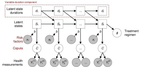
Figure 2: Proposed variable-duration copula hidden Markov model. Shown is the VDC-HMMX for a given patient $i$ (subscript omitted for better readability). Health measurements are observable (gray shading), whereas the latent states are not (these reflect the different trajectory phases).

3.3 Variable-Duration Component

As part of the variable-duration component in our VDC-HMMX, we now specify the transition probabilities $\gamma_{it}^{j\to k}$ based on further controls $x_{it}$ (e. g., patient-individual risk factors) and the duration spent in a latent state. The latter is of particular importance: It allows us to consider the past latent state sequence. Thereby, we overcome limitations due to the Markov property that are inherent to naïve HMMs (Yu 2010). Specifically, naïve HMMs assume that transition probabilities are independent of time and they are therefore treated as stationary. However, as argued above, there is evidence in medical research that this assumption is too restrictive and, instead, our setting demands that the transition probability depends on the time spent in the current state. This is formalized in the variable-duration component of our VDC-HMMX.

We make use of the following notation. Formally, the transition probability $\gamma_{it}^{j\to k}$ defines the probability of patient $i$ moving at time $t$ from a latent state $j$ to a latent state $k$. To this end, let $d_{it}(j)$ denote the prior duration (in weeks) that patient $i$ spent in the latent state $j$ at a certain time $t$. It gives the consecutive duration since the last transition. Analogous to the latent state, the duration $d_{it}(j)\in\left\{1,\ldots,t\right\}$ is also latent. This prevents us from simply inserting $d_{it}(j)$ in the model, since it is not directly observable. Instead, one requires an approach where both latent states and latent state durations are modeled jointly, as in a variable-duration component.

The variable-duration component distinguishes two cases when modeling the transition probability $\gamma_{it}^{j\to k}$: (1) The patient remains in the current latent state, i. e., $j=k$. We refer to this as a recurrent transition. This occurs with probability $\gamma_{it}^{j\to j}$. (2) The latent state of the patient changes to a different state, i. e., $j\neq k$. We refer to this as a non-recurrent transition, which occurs with probability $1-\gamma_{it}^{j\to j}$.

Both the recurrent and non-recurrent transitions are modeled in the variable-duration component, while further incorporating additional sources of heterogeneity $x_{it}$, such as risk factors or previous health measurements. As as suggested in previous works (e. g., Netzer et al. 2008), we model the risk factors inside the transitions via a multinomial logit function. The multinomial logit considers the current state as a base case and then compares it to the probability of moving to a different state. This allows the propensity of moving between states to differ based on patient characteristics. Formally, we specify

$$\gamma_{it}^{j\to k}=P\left(S_{i,t+1}=k\mid S_{i,t}=j,d_{it}(j)\right)=\begin{cases}\cfrac{1}{1+\sum_{l\neq k}\exp(\delta_{jl}+\omega_{jl}d_{it}(j)+{x}_{it}^{T}\beta_{jl})},&\text{ for }k=j,\\ \cfrac{\exp(\delta_{jk}+\omega_{jk}d_{it}(j)+{x}_{it}^{T}\beta_{jk})}{1+\sum_{l\neq k}\exp(\delta_{jl}+\omega_{jl}d_{it}(j)+{x}_{it}^{T}\beta_{jl})},&\text{ for }k\neq j.\end{cases}$$ (2)

with intercepts ${\delta}_{jl}$ and coefficients $\omega_{jl}$ and ${\beta}_{jl}$ for $j,l=1,\ldots,\varsigma$. Consistent with Netzer et al. (2008), we set the parameters ${\beta}_{jj}$, ${\omega}_{jj}$ and ${\delta}_{jj}$ to zero to ensure identifiability of the parameters.

The above variable-duration component has multiple implications. First, the dependence on the latent state duration $d_{it}$ essentially relaxes the Markov property that limits naïve HMMs. Second, the transition probabilities are no longer time-homogeneous, as they depend on the prior duration in the current state. This holds true for both recurrent and non-recurrent transitions. Third, the variable-duration component allows states to become more “sticky” with $d_{it}(j)$. This is captured via the parameters $\omega_{jl}$ for $j\neq l$. If $\omega_{jl}$ is positive, the probability of a non-recurrent transition increases with a longer duration $d_{it}(j)$. If $\omega_{jl}$ is negative, a recurrent transition becomes more likely. Fourth, our specification benefits from direct interpretability, as we can identify the extent to which risk factors influence disease dynamics. Fifth, if $\omega_{jl}$ are all held at zero, the naïve HMM becomes a special case of our VDC-HMMX. Because of this, the likelihood of the HMM differs from that of our VDC-HMMX and, in order to estimate our model, must be derived.

Our VDC-HMMX model is estimated via Markov chain Monte Carlo (MCMC) sampling by deriving the likelihood

$$L=\prod_{i=1}^{N}P\left(y_{i1},\ldots,y_{iT}\right)=\prod_{i=1}^{N}\sum_{s_{1}=1}^{\varsigma}\sum_{s_{2}=1}^{\varsigma}\cdots\sum_{s_{T}=1}^{\varsigma}\left[P(S_{i1}=s_{1})\times\prod_{t=2}^{T}\gamma_{it-1}^{s_{t-1}\to s_{t}}\times\prod_{t=1}^{T}b_{s_{t}}(Y_{it}=y_{it})\right].$$ (3)

If we assume the margins of the observations $Y_{it}$ to be independent given the current latent state $S_{it}$, the above equation simplifies to

$$L=\prod_{i=1}^{N}\sum_{s_{1}=1}^{\varsigma}\sum_{s_{2}=1}^{\varsigma}\cdots\sum_{s_{T}=1}^{\varsigma}\left[P(S_{i1}=s_{1})\times\prod_{t=2}^{T}\gamma_{it-1}^{s_{t-1}\to s_{t}}\times\prod_{t=1}^{T}\prod_{k=1}^{m}b_{s_{t}}^{(k)}(Y_{it}^{(k)}=y_{it}^{(k)})\right].$$ (4)

By sampling from the likelihood $L$, we can thus directly estimate $\omega_{jl}$ from the data. In practice, a direct evaluation of the likelihood is computationally intractable and we thus apply the forward algorithm for an efficient calculation (Yu 2010). All estimation details are reported in the supplements.

3.4 Copula Approach for Modeling Dependence Structures

3.4.1 Overview.

Health management commonly monitors the progression of diseases along multiple symptoms (e. g., Jensen et al. 2015); however, symptoms are usually not unrelated. Rather, they co-occur in a specific manner: (1) either all (or almost all) symptoms are absent when the patient has recovered, or (2) the condition is indicated by some – but not necessarily all – symptoms due to differences in how patients respond to a disease. For instance, patients with stable low back pain experience an absence of both pain and activity limitation, whereas acute low back pain is usually characterized by severe pain or activity limitation, though rarely both. In other words, the absence of one symptom makes it more likely that other symptoms will also be absent. Altogether, this results in a lower tail dependence among health measurements that must be modeled accordingly.

In this section, we provide a rigorous approach for modeling the dependence structure among multivariate (discrete) emissions. The dependence structure represents a clear difference to the naïve HMM where independence is assumed. Formally, in the above likelihood, independence was needed in order to rewrite $b_{s}(Y_{it}=y)$ in the likelihood as $\prod_{k=1}^{m}b_{s}^{(k)}(Y_{it}^{(k)}=y_{k})$, i. e., when moving from Equation 3 to Equation 4. Hence, in order to consider a dependence structure, we now need to derive a new likelihood. To accomplish this, the likelihood of our VDC-HMMX is updated by proceeding in two steps. We first formalize the distribution function $b_{s}(Y_{it}\leq y)=P(Y_{it}\leq y\mid S_{it}=s)$ via a copula function $C_{s}$ operating on the marginal distribution functions. Here the copula function $C_{s}$ provides a flexible tool for modeling the nature of the dependence structure (i. e., a lower tail dependence). Second, we use the resulting distribution function to derive the new emission $b_{s}(Y_{it}=y)$ subject to a copula-based dependence structure. The new emission is then simply inserted into the likelihood from Equation 3, so that we estimate the model parameter by applying the previous MCMC sampling technique.

3.4.2 Copula-Based Distribution Function.

Let $C_{s}(\cdot,\ldots,\cdot)$ denote a copula function (Joe 1997). A copula is a generalized correlation function, which allows for a stronger dependence in certain parts of the distribution. Formally, it links the individual marginal distributions of an $m$-dimensional input to a joint cumulative distribution function, while introducing a desired dependence structure between the margins. Depending on which copula is chosen, $C_{s}$ might be parameterized by further variables that, for instance, control for the strength of the dependence. In our work, the parameters are modeled as state-specific, which is indicated in the copula by the subscript $s$. A state-specific $C_{s}$ is needed for our research, as there should be different dependencies across states (e. g., a stronger dependence of the tails in acute as opposed to stable states). The copula can be freely chosen; however, our setting demands a lower tail dependence due to the specific characteristics of health measurements and, hence, we use a survival Gumbel copula. This choice is discussed later.

Formally, a copula $C\colon[0,1]^{m}\to[0,1]$ is an $m$-dimensional cumulative distribution function. For every $m$-dimensional cumulative distribution $F\colon\mathbb{R}^{m}\to[0,1]$ with marginal cumulative distribution functions $F_{1},\ldots,F_{m}$, the existence of a copula function, such that $F(x_{1},\ldots,x_{m})=C(F_{1}(x_{1}),\ldots,F(x_{m}))$, is guaranteed by Sklar’s theorem (Joe 1997). If all margins are continuous, the copula $C$ is unique. However, the same does not hold if one of the margins is discrete (Genest and Nešlehová 2007), as in our case.

We now use the copula to formalize a dependence structure between the marginal distribution of $b_{s}(Y_{it}\leq y)$. This is given by

$$b_{s}(Y_{it}\leq y) =P(Y_{it}^{(1)}\leq y_{1},\ldots,Y_{it}^{(m)}\leq y_{m}\mid S_{it}=s)$$ (5)

$$=C_{s}\left(P(Y_{it}^{(1)}\leq y_{1}\mid S_{it}=s),\ldots,P(Y_{it}^{(m)}\leq y_{m}\mid S_{it}=s)\right).$$ (6)

Here the dependence between observations $y_{1},\ldots,y_{m}$ is modeled by “linking” the separate marginal distribution functions $P(Y_{it}^{(1)}\leq y_{1}\mid S_{it}=s)$, …, $P(Y_{it}^{(m)}\leq y_{m}\mid S_{it}=s)$ inside the copula (e. g., Nikoloulopoulos 2013). Based on the distribution function $b_{s}(Y_{it}\leq y)$, we derive the new emission $b_{s}(Y_{it}=y)$ in the following.

3.4.3 Copula-Based Emissions.

For a given copula, our objective is to derive a new emission $b_{s}(Y_{it}=y)$. The new emission is then integrated into the likelihood of our VDC-HMMX, which allows us to estimate the model under a given dependence structure.

For discrete observations, as in our study, we derive the new emission via

$$b_{s}(Y_{it}=y) =P(Y_{it}^{(1)}=y_{1},\ldots,Y_{it}^{(m)}=y_{m}\mid S_{it}=s)$$ (7)

$$=\sum_{i_{1}=0}^{1}\cdots\sum_{i_{m}=0}^{1}(-1)^{i_{1}+\ldots+i_{m}}\,P(Y_{it}^{(1)}\leq y_{1}-i_{1},\ldots,Y_{it}^{(m)}\leq y_{m}-i_{m}\mid S_{it}=s)$$ (8)

$$=\sum_{i_{1}=0}^{1}\cdots\sum_{i_{m}=0}^{1}(-1)^{i_{1}+\ldots+i_{m}}\,C_{\nu_{s}}\left(P(Y_{it}^{(1)}\leq y_{1}-i_{1}\mid S_{it}=s),\ldots,P(Y_{it}^{(m)}\leq y_{m}-i_{m}\mid S_{it}=s)\right).$$ (9)

Here Equation 8 follows from the fact that the marginal likelihood can be derived from the corresponding distribution function as $b_{s}^{(k)}(Y_{it}^{(k)}=y_{k})=P(Y_{it}^{(k)}\leq y_{k}\mid S_{it}=s)-P(Y_{it}^{(k)}\leq y_{k}\mid S_{it}=s)$, $k=1,\ldots,m$. Equation 9 is simply the result of inserting the distribution function from above. For continuous or mixed observations, the derivation can be readily extended (see Onken and Panzeri 2016).

The resulting model is estimated as follows. The new emission $b_{s}(Y_{it}=y)$ is used to update the likelihood from our VDC-HMMX. That is, we simply replace $b_{s}(Y_{it}=y)$ inside Equation 3, thereby yielding the new likelihood function for our VDC-HMMX. Based on the likelihood, the model parameters can be simply obtained via MCMC sampling, as detailed in the supplements.

3.4.4 Choice of Copula Function.

Our copula $C_{s}$ should accommodate tail dependence, so that an absence of symptoms appears jointly. In order to model this behavior, we draw upon a survival Gumbel copula. For $u,v\in[0,1]$, it is given by

$$C_{s}(u,v)=u+v-1+\exp\left[-\left((-\log(1-u))^{\nu_{s}}+(-\log(1-v))^{\nu_{s}}\right)^{\frac{1}{\nu_{s}}}\right],$$ (10)

where the parameter $\nu_{s}\geq 1$ controls the strength of the tail dependence. It can be shown that the survival Gumbel copula has positive lower tail dependence for $\nu_{s}>1$ and zero upper tail dependence for all $\nu_{s}$ (see, e. g., Joe 1997). For the special case of $\nu_{s}=1$, the survival Gumbel copula reduces to independent observations.

For comparison, we also later experiment with other dependence structures (see supplements). On the one hand, we use no copula. This ensures independence. On the other hand, we use the Ali-Mikhail-Haq copula in order to test for a symmetric dependence structure. It is given by $C_{s}(u,v)=u\,v\,(1-\nu_{s}^{\prime}(1-u)(1-v))^{-1}$ with an additional parameter $\nu_{s}^{\prime}\in[-1,1)$. Here the symmetric dependence structure follows from its multiplicative form. However, our numerical experiments later confirm that the Gumbel copula is superior.

Employing a copula approach has multiple benefits. First, it is highly flexible as different copula functions for modeling dependence structure can be chosen. The copula functions can even be parameterized. Second, a copula approach requires fairly little a priori knowledge, as parameters are estimated from data. Third, using a copula approach generalizes to both continuous and, in particular, discrete observations. The latter prohibits the use of alternative approaches from the literature, where both marginal distributions and observations must originate from the same family of distributions.

3.5 Inferring Treatment Regimens

Our VDC-HMMX is used to recommend treatment regimens in a two-step procedure. First, we compute the latent states specific to a patient profile. Formally, we recover the latent state sequence $S_{it}$ from the observed health measurements $Y_{i1},\ldots,Y_{it}$ conditional on a given risk profile $x_{i1},\ldots,x_{it}$. Second, the recovered latent state is mapped onto one of the three treatment regimens $\phi_{it}\in\{\text{acute},\text{unstable},\text{stable}\}$. To this end, the recommended treatment regimen is determined via

$$\argmax\limits_{\phi_{it}}\;P(\phi_{it}\mid Y_{i1},\ldots,Y_{it},x_{i1},\ldots,x_{it})$$ (11)

$$= \argmax\limits_{\phi_{it}}\;=P(\phi_{it}\mid S_{it}^{\ast})\quad\text{with }\quad S^{\ast}_{it}=\argmax_{s}P(S_{it}=s\mid Y_{i1},\ldots,Y_{it},x_{i1},\ldots,x_{it})$$ (12)

using the observed frequencies of ground-truth labels $\phi_{it}$ from the training data. Note that the patient-specific risk profile $x_{it}$ (e. g., past treatments, age, gender) is explicitly considered in the latent dynamics of our VDC-HMMX, and, owing to this fact, the predictions are personalized to a patient’s risk profile. For instance, a patient with a high body mass index has a transition mechanism different from that of a patient with a low body mass index, because of which the latent state sequence and final prediction are also different.

We emphasize that the previous procedure is inherently dynamic; it considers the inputs only from time step 1 until a given $t$. Once a new health measurements becomes available, the previous procedure must be repeated. The predictions are then compared against the expert labels, which were, however, obtained with post-hoc knowledge. That is, the experts have made their annotation by considering the progression until $T>t$ and thus beyond the time step $t$. Altogether, this yields the corresponding framework for a dynamic “on-line” evaluation:

for $t=1,\ldots$ do

       Receive new health measurement $Y_{it}$

       Compute $S_{it}^{\ast}=P(S_{it}=s\mid Y_{i1},\ldots,Y_{it},x_{i1},\ldots,x_{it})$ for $s=1,\ldots,\varsigma$ using the forward algorithm

       Determine treatment regimen $\phi_{it}$

       Compare $\phi_{it}$ against post-hoc annotation from experts

end for

Formally, we recover patient-specific latent states by determining the likeliest state $S_{it}$ conditional on $Y_{i1},\ldots,Y_{it}$. The latent state depends on the latent state duration, which again depends on multiple previous latent states, thus driving the overall computational complexity. An efficient computation scheme is is obtained via the forward algorithm (Yu 2010).

4 Longitudinal Study of Low Back Pain

Our empirical model for personalized treatment planning is validated based on a longitudinal cohort study of patients with non-specific low back pain. Non-specific low back pain represents a chronic condition for many subjects, who experience a recurrent, variable, and often long-lasting course. Low back pain is globally responsible for the greatest number of years lived with disability (GBD 2017) and thus burdens both patients and society with extensive costs, while its causes are widely unknown (Foster et al. 2018, Hartvigsen et al. 2018). Health researchers comprised part of the authorial team and ensured that both the above model development and the following evaluation fulfill clinical standards.

4.1 Study Design

This work builds upon an extensive, longitudinal, 52-week study of 928 patients. The actual design of the study was developed and undertaken by experts from the medical domain in a manner that adheres to common conventions and regulations of clinical studies (Kongsted et al. 2015, Nielsen et al. 2016, 2020). The data was obtained based on a prospective observational cohort study. The clinical study was conducted between September 2010 to January 2012 in Southern Denmark. Eventually, the duration of the study was set at one year, as this exceeds the usual length of low back pain episodes by several times (Kongsted et al. 2015). Hence, for most patients, a length of 52 weeks is sufficient to observe multiple episodes with severe symptoms. All general practitioners in that region were invited to participate and recruit participants. To collect longitudinal data, an IT-based health monitoring system was used to send weekly text messages to patients asking for their pain level and activity limitations, and the patients responded via text message. The use of this IT-enabled system for health tracking allowed the study to scale to both a large number of patients and long study period

The cohort fulfilled the following criteria: between 18–65 years of age, possessed a mobile phone, could read sufficiently well to answer the survey questions, and were not pregnant or suspected of having a serious pathology that required referral for acute surgical assessment. A healthcare professional had diagnosed the subjects with non-specific low back pain based on each patient’s history and a physical examination.

The study consists of three components as follows. (1) An extensive upfront survey collected information on various risk factors that describe the between-patient heterogeneity. These variables are detailed later. We use the term “risk factor”, while, from a medical perspective, these variables are not describing the onset but rather the course of a disease. (2) The longitudinal progression was monitored over the course of 52 weeks. Patients were asked to report their weekly levels of experienced pain and activity limitation. (3) The longitudinal data was subsequently annotated by three medical experts, physicians with experience in treating low back pain who were also trained in the trajectory framework. For each patient and week, the medical experts then stated whether they would recommend an acute, unstable, or stable treatment regimen. The annotations from the medical experts were aggregated by the majority vote. Kendall’s tau amounts to $0.89$ and, hence, the annotations revealed considerable between-annotator agreement. The annotations are considered the ground truth for all subsequent evaluations. We emphasize that the medical experts had unique post-hoc knowledge due to our longitudinal dataset when they inspected trajectories, whereas our decision rules are later evaluated in an on-line manner to reflect the partial information (until a certain time step $t\leq T$) that would be available to health professionals in practice.

4.2 Data Description

The course of low back pain was monitored using two health measurements $Y_{it}$: (1) The average pain intensity, which was collected each week on the so-called NRS scale (Breivik et al. 2008). This represents the default procedure for a valid and reliable measurement of pain in clinical research. It measures pain on a scale from 0 (i. e., no pain) to 10 (i. e., worst pain imaginable). (2) Activity limitation was measured based on the number of days characterized by activity limitation during the previous week and thus ranges from 0 to 7 days.

The variable $x_{it}$ is used to describe the between-patient heterogeneity. It is obtained by appending the following covariates. First, treatments are likely to be associated with the progression of a disease. Here we follow Yan and Tan (2014) and control for the fact that interventions can be linked to state transitions. For low back pain, we expect treatments (e. g., massage, acupuncture) to affect the latent state within a few days and thus fed the variable into the model without time lag (however, this may be different for other chronic diseases). Second, we include a set of nine further patient-specific risk factors (see Table 3): age, height, BMI, general health, gender, leg pain, duration of current pain episode, number of previous episodes, and physical work load. These risk factors have been carefully chosen based on clinical considerations (i. e., they entail a high prognostic capacity with regard to the future course of low back pain). Of note, duration of current pain episode and number of previous episodes should not be confused with the phase (acute, unstable, stable), which is a latent variable. Third, we include the previous health measurements $Y_{i,t-1}$. Such a first-order structure is informed by prior theory in medical research on modeling intrapersonal pain variability (Mun et al. 2019).

Out of the original 928 patients in our study, we excluded 76 due to their failure to participate in the weekly monitoring, as well as 5 patients who reported the same pain intensity in each of the 52 weeks. This yields a final sample of 847 distinct patients. All of our models were trained on a random subset of $600$ patients, while the remaining $247$ samples represent our test set in order to evaluate the accuracy of treatment regimens that were correctly identified.

4.3 Summary Statistics

Table 3 lists summary statistics for our risk factors. For instance, in our study, $62.55\text{\,}\mathrm{\char 37\relax}$ of all low back pain episodes lasted up to 2 weeks, $13.69\text{\,}\mathrm{\char 37\relax}$ from 2–4 weeks, and $10.68\text{\,}\mathrm{\char 37\relax}$ from 1–3 months.

The course of low back pain is characterized by considerable variability. Pain sometimes vanishes temporarily, but often persists in the long run. Furthermore, we regularly note jumps from a pain intensity of zero to higher values (and vice versa). Examples are presented in Figure 1. As a consequence, we also observe that the annotations from our medical experts are highly variable (i. e., each trajectory was annotated, on average, with more than two different treatment regimens).

Both health measurements (pain level and activity limitation) are highly correlated (correlation coefficient of $0.65$ as measured by Kendall’s $\tau_{b}$). Moreover, low values of pain intensity are reported considerably more often by patients then severe ones. For instance, $57.0\text{\,}\mathrm{\char 37\relax}$ of all reported pain levels correspond to a rating of zero (i. e., no pain). This results in a mean value of $1.45$ with a standard deviation of $2.21$. The activity limitation follows analogously. Here the mean value amounts to $0.79$ with a standard deviation of $1.85$. However, in terms of activity limitation, we observe a substantial number of patients reporting the maximum value of $7$. Severe activity limitation is frequent even when the pain intensity is moderate or low.

Table 3: Summary Statistics of Risk Factors.

Continuous risk factors	Statistic	Value
Age (in years)	Range	18–65
	Mean	43.20
	Std. dev.	11.44
Height (in cm)	Range	153–201
	Mean	175.99
	Std. dev.	8.86
Body mass index (BMI)	Range	18–59
	Mean	26.26
	Std. dev.	4.66
General health	Range	0–100
(EQ-5D scale)	Mean	67.57
	Std. dev.	20.49
Categorical risk factors	Levels	Relative frequencies
Gender	Female	$45.93\text{\,}\mathrm{\char 37\relax}$
	Male	$54.07\text{\,}\mathrm{\char 37\relax}$
Severity of leg pain	No pain	$41.98\text{\,}\mathrm{\char 37\relax}$
	Mild pain	$33.95\text{\,}\mathrm{\char 37\relax}$
	Moderate-severe pain	$24.07\text{\,}\mathrm{\char 37\relax}$
Duration of current episode	0–2 weeks	$62.55\text{\,}\mathrm{\char 37\relax}$
	2–4 weeks	$13.69\text{\,}\mathrm{\char 37\relax}$
	1–3 months	$10.68\text{\,}\mathrm{\char 37\relax}$
	More than 3 months	$13.09\text{\,}\mathrm{\char 37\relax}$
Number of previous episodes	None	$16.11\text{\,}\mathrm{\char 37\relax}$
	1–3	$34.62\text{\,}\mathrm{\char 37\relax}$
	More than 3	$49.28\text{\,}\mathrm{\char 37\relax}$
Physical work load	Sitting	$24.03\text{\,}\mathrm{\char 37\relax}$
	Sitting and walking	$35.74\text{\,}\mathrm{\char 37\relax}$
	Light physical work	$19.93\text{\,}\mathrm{\char 37\relax}$
	Heavy physical work	$20.30\text{\,}\mathrm{\char 37\relax}$
Longitudinal monitoring	Statistic	Value
Pain intensity (NRS scale; 0–10)	Mean	1.45
	Std. dev.	2.21
Activity limitation (in days; 0–7)	Mean	0.79
	Std. dev.	1.85
Interventions (at week level; yes/no)	Yes	$1.92\text{\,}\mathrm{\char 37\relax}$
	No	$98.08\text{\,}\mathrm{\char 37\relax}$

4.4 Dependence Structure of Observations

We finally investigate the dependence structure between pain intensity and activity limitation. The association between pain intensity and activity limitation amounts to $0.65$ as measured by Kendall’s $\tau_{b}$, which is statistically significant at the $0.1\text{\,}\mathrm{\char 37\relax}$ threshold. Section 4.4 reports the relative frequency of pain intensities conditional on the activity limitation (in %). Thereby, we can investigate which values frequently appear together. We observe a strong dependence between both dimensions that becomes especially evident at the lower tails. For example, we generally observe low pain levels given a low activity limitation. However, when conditioning on the maximum activity limitation, we find a wide range of pain intensities (between $2$ and $8$).

Dependence Structure Between Health Measurements. Pain intensity Activity limitation 0 1 2 3 4 5 6 7 8 9 10 0 77.71 4.46 7.09 5.41 2.79 1.53 0.63 0.27 0.10 0.02 0.01 1 0.51 8.98 25.38 25.53 16.14 11.32 5.69 3.91 1.98 0.30 0.25 2 0.12 2.85 17.47 22.71 19.92 16.31 10.19 5.42 4.25 0.64 0.12 3 0.09 1.48 8.68 20.14 20.23 22.14 11.63 8.68 5.21 1.22 0.52 4 0.13 0.80 5.59 9.32 19.97 26.36 16.91 11.19 7.59 1.86 0.27 5 0.29 1.17 5.98 7.43 12.10 23.62 16.18 16.76 12.83 2.62 1.02 6 0.00 0.00 5.30 3.03 6.44 15.91 25.00 17.05 19.70 3.79 3.79 7 0.14 5.73 11.09 10.57 11.88 16.06 13.34 13.95 11.51 2.58 3.15 Notes: The table reports the relative frequency of pain intensities conditional on the activity limitation (in %). Thereby, we can investigate which values frequently appear together. We note a strong dependence between both dimensions that becomes especially evident at the lower tails. Rows are standardized to sum to one. All cells with values above $10$ are shaded in light gray; above 25 in dark gray.

4.5 Current Practice in Managing Low Back Pain

Low back pain is known for the recurrent nature of its course (Foster et al. 2018, Hartvigsen et al. 2018). This is also reflected in the treatment regimens that are conventionally practiced (Foster et al. 2018, Traeger et al. 2019). For example, in a stable treatment regimen, patients primarily receive a combination of pain self-management, education, and graded exercise therapy. As with other chronic diseases, the treatment regimens aim at stabilizing the current trajectory phase. As is common in clinical research, the effectiveness of the different models is compared by computing the quality-adjusted life years (QALYs). Here we use the disability weights from Hoy et al. (2014).

Providing care for low back pain entails the following costs (Whitehurst et al. 2012): A stable treatment regimen was estimated to have an annual costs of only USD 208.57 (GBP $160.44$) per patient. Unstable and acute treatment regimens often involve physical therapies, and their yearly costs per patient are thus considerably larger, amounting to USD 374.14 (GBP $287.80$) and USD 464.71 (GBP $357.47$), respectively. Costs associated with managing low back pain usually accumulate over an extensive period, as this disease is known for causing the largest number of years lived with disability (GBD 2017).

Choosing a treatment regimen that does not match the trajectory phase is considered ineffective when following the clinical guidelines (Larsen 2017); it fails to adapt to the underlying disease dynamics as it targets patients from a different cohort. For instance, pain self-management is highly effective in a stable trajectory phase, yet can barely maintain the course during an unstable or acute phase. Similarly, medication for acute treatment regimens should be avoided for less severe regimens due to strong side-effects (Traeger et al. 2019). Analogous to Kazemian et al. (2019), we base our evaluations on the following cost structure, where costs are accumulated over all misidentified treatment regimens (i. e., the absolute deviation between suggested and needed treatment regimen, i. e. between the used and the post-hoc required treatment costs treatment costs). To this end, more comprehensive treatment regimens than necessary are counted as over-treatment, while less comprehensive treatment regimens than necessary are counted as under-treatment.

4.6 Baselines

As for all chronic diseases, health professionals are advised to consider the past course of the disease in their decision-making. Oftentimes, however, this information is not readily available due to a lack of longitudinal monitoring. To formalize decision-making in current practice, we consider a set of decision rules that vary in terms of the extent to which the past course is considered. As in earlier research (e. g., D’Amato et al. 2000, Ibrahim et al. 2016), we develop different myopic decision rules and extend them with data from the patient history (ordered by increasing complexity):

1. Myopic decision rule (symptoms only). Analogous to Ibrahim et al. (2016), we develop a myopic decision rule. Here we use a generalized linear model to predict the annotated regimen from the current health measurements $Y_{it}$ (and a pain-disability interaction term).

2. Myopic decision rule (risk factors). In order to accommodate between-patient heterogeneity, this model incorporates both $Y_{it}$ (with interaction term) and risk factors $x_{it}$ in a generalized linear model.

3. Dynamic decision rule (moving average). Here we extend the previous decision rule, so that it is additionally fed with the past history of health measurements via a moving average, i. e., $\bar{Y}_{it}=\frac{1}{t-1}\sum_{\tau=1}^{t-1}Y_{i\tau}$.

4. Dynamic decision rule (ARMA). This model considers all of the above predictors and, in addition, three autoregressive terms.

5. LSTM. As another sequential baseline, we also implemented a recurrent neural network (i. e., a long short-term memory network, LSTM for short). This model is trained in a supervised manner analogous to the other baselines (cf. Kraus et al. 2020).

These models are based on supervised learning and, in contrast to our VDC-HMMX, are thus trained via expert annotations.

5 Model Estimation

Here we perform a model selection to choose our preferred model specification. In particular, we compare our VDC-HMMX against other variants without variable-duration component as well as without copula to demonstrate the effectiveness of our proposed model. Due to space, additional details are in the Online Appendix.

5.1 Model Variants

We compare the following model variations that differ in the underlying personalization (all of them make use of our copula approach; additional model variations are discussed as part of the robustness checks):

1. Variable-duration HMMX. This corresponds to our VDC-HMMX but it has no copula. As such, the different health measurements are assumed as being independent.

2. Copula HMMX. This corresponds to our VDC-HMMX but without a variable-duration component. This model thus follows other HMMs in management literature (e. g., Martino et al. 2018, Yan and Tan 2014).

3. VDC-HMMX. This corresponds to the proposed variant specified above.

We base our model selection on the out-of-sample performance. For treatment planning, this yields a model that generalizes well to unseen patients. We follow the latest recommendations in Bayesian modeling (Gelman et al. 2014) and use the out-of-sample log point-wise predictive density (lpd). Different from the deviance information criterion (DIC) or the Akaike information criterion (AIC), the lpd is beneficial as it considers the whole posterior distribution. We also report approximate metrics of the lpd, namely the widely applicable information criterion (WAIC) and the leave-one-out cross-validation information criterion (LOO). Furthermore, we state the in-sample lpd in order to provide an indication, when overfitting occurs. All values are measured on the deviance scale such that smaller values indicate a better model fit.

5.2 Model Selection

Section 5.2 presents the results. The best out-of-sample lpd is obtained by the VDC-HMMX. It outperforms both the variable-duration HMMX and the copula HMMX, thereby confirming that a combination of variable-duration component and copula within an HMMX is beneficial.

We make further observations. First, the the change from the copula HMMX to our VDC-HMMX (i. e., $862.59$ in lpd) is larger than the change between a naïve VDC-HMM without risk factors and our VDC-HMMX (i. e., the difference is only $116.00$). In other words, the improvement gained by including the variable-duration component is larger than that gained by including risk factors. This highlights the importance of relaxing the Markov property for our research and accommodate a variable-duration component.

Second, an out-of-sample lpd of 40234.32 is obtained for the variable-duraton HMMX without copula, that is, when assuming independence among health measurements. In comparison, a value of 39966.27 is registered for our VDC-HMMX. This amounts to an improvement of $268.05$. To put this into context, this improvement is more than twice as large as the performance gained through the inclusion of risk factors (i. e., the improvement of the VDC-HMMX over a naïve VDC-HMM amounts to only $116.00$). This thus highlights the importance of considering a copula approach.

In sum, our proposed VDC-HMMX is to be preferred, and, hence, we draw upon the VDC-HMMX in all subsequent analyses.

Model Selection. Expected lpd True lpd Model LOO WAIC In-sample Out-of-sample Variable-duration HMMX (i. e., no copula) $89742.66$ $89737.34$ $89091.24$ $40234.32$ Copula HMMX (i. e., no variable-duration) $91725.22$ $91701.80$ $90728.74$ $40828.86$ Proposed VDC-HMMX $89402.53$ $89400.83$ $88669.65$ $\bm{39966.27}$ Lower = better (best out-of-sample performance in bold)

5.3 Estimation Results

The posterior means of the emission probabilities are listed in Section 5.3 (i. e., marginal distributions $b_{s}^{(k)}$). As expected, we observe a strong lower-tail dependence between pain intensity and activity limitation. Furthermore, the three latent states match the different trajectory phases: (1) the stable state reveals the nearly complete absence of symptoms as demonstrated by both low pain intensity and almost no activity limitation; (2) the unstable state reflects dispersed health measurements; and (3) the acute state shows mostly severe health measurements. Altogether, this suggests that our model has successfully encoded the trajectory phases in the latent states.

Mean Posterior Emission Probabilities (i. e., Marginal Distributions $b_{s}^{(k)}$).

Notes: This table presents the mean posterior emission probability (in %) for each latent state. We highlight posterior probabilities greater than $1\text{\,}\mathrm{\char 37\relax}$ and $5\text{\,}\mathrm{\char 37\relax}$ in light and dark gray, respectively. As a result, the latent states can be interpreted as stable, unstable, and acute trajectory phases.

6 Model Performance

We now utilize our proposed VDC-HMMX for personalizing treatment planning.

6.1 Accuracy of Inferred Treatment Regimens

This section assesses the relative frequency with which clinical guidelines for choosing an effective treatment regimen are obtained. Accordingly, we compute the accuracy of how often the correct treatment regimen was identified. The data-driven approaches are evaluated based on the dynamic on-line framework. That is, they receive a health measurement at time $t$ and must then suggest a treatment regimen before the health measurement from the next week $t+1$ becomes available. As the course of symptoms is highly variable, it renders treatment planning considerably more challenging. In comparison, the ground truth annotations are provided by the medical experts who were privy to the complete disease progression for annotation and, hence, benefited from post-hoc knowledge. If one had – hypothetically – post-hoc knowledge of the disease progression, one could always choose the best treatment regimen in medical practice, thereby identifying the correct treatment regimen with 100% accuracy and thus removing all costs from over-/under-treatment. However, in medical practice, this is not possible as it requires post-hoc knowledge.

We compare the performance of our VDC-HMMX against a range of baselines (see Section 4.6). Section 6.1 reports the F1 score (the harmonic mean of precision and recall) and the balanced accuracy (due to the uneven distribution of treatment regimens). We first study symptom-based classifiers as our prime baseline. Here the decision rules that mimic current practice register an overall balanced accuracy of $72.63\text{\,}\mathrm{\char 37\relax}$ (myopic decision rule, i. e., current symptoms only) and $74.25\text{\,}\mathrm{(}$ARMA). These performance values already highlight challenges that health professionals face when managing chronic diseases: Identifying an effective treatment regimen without knowledge of a patient’s health trajectory is difficult. Similar findings from qualitative research have been reported earlier (e. g., Burton 2000, Corbin and Strauss 1991).

In comparison, our data-driven model attains an overall balanced accuracy of $83.65\text{\,}\mathrm{\char 37\relax}$. Hence, it bolsters the overall accuracy by $9.49$ percentage points. For all baseline decision rules, the improvement is statistically significant at the 0.001 significance threshold. In particular, our data-driven model is more accurate when acute treatment regimens are needed. Hence, it facilitates care provision for patients with severe conditions.

The LSTM registers a balanced accuracy of 81.33 and an F1 score of 73.91. Hence, it outperforms the other baselines mimicking current practice but, in comparison to our VDC-HMMX, it is still inferior by a large margin. On top of that, the long short-term memory is regarded as a black-box and, based on discussions with healthcare professionals, its use was discouraged. In our case, the tuned network architecture has $6703$ parameters, which is $43$ times larger than the parsimonious formulation of the VDC-HMMX. Due to this fact, the use of such a recurrent neural network is further limited in practice.

Accuracy in Inferring Treatment Regimens. F1 score Balanced accuracy Model Overall Stable Unstable Acute Overall Stable Unstable Acute Baselines     Myopic decision rule (symptoms only) $65.86$ $84.20$ $43.32$ $70.06$ $72.63$ $76.25$ $62.82$ $78.81$     Myopic decision rule (risk factors) $67.47$ $84.96$ $45.62$ $71.84$ $73.66$ $77.53$ $63.86$ $79.58$     Dynamic decision rule (moving average) $67.23$ $85.54$ $52.82$ $63.33$ $74.00$ $79.02$ $67.59$ $75.40$     Dynamic decision rule (ARMA) $67.24$ $85.81$ $53.48$ $62.43$ $74.25$ $79.54$ $67.95$ $75.25$     LSTM $73.91$ $91.00$ $64.30$ $66.43$ $81.33$ $88.81$ $74.68$ $80.40$ Proposed VDC-HMMX $77.02$ $90.69$ $66.14$ $74.24$ $83.65$ $88.95$ $76.02$ $85.98$ Improvement over best baseline (in percentage points) $9.78$ $4.88$ $12.66$ $3.68$ $9.40$ $9.41$ $8.07$ $6.99$ Stated: macro-averaged overall and class-specific performance; balanced accuracy in %.

6.2 Cost-Effectiveness

Section 6.2 compares the effectiveness based on the improvement in QALY over “no treatment” across different models. As the results show, our model outperforms the best baseline by 12.97 percentage points. This directly reflects benefits for patients’ health provided by our data-driven approach to treatment planning. We further provide a cost analysis of over- and under-treatment. Hence, for the given decision rules, we accumulate over the absolute deviation in costs between suggested and expert-annotated treatment regimens, thereby following common guidelines in chronic care (Larsen 2017). Compared to our model, the LSTM is fairly similar in terms of total costs but has a substantially lower QALY improvement. The different interpretable baseline models yield fairly similar annual over-/under-treatment costs of, on average, USD 37.69 per patient. For comparison, our model implies annual over-/under-treatment costs of USD $23.80$ per patient. This amounts to an overall improvement of $35.71\text{\,}\mathrm{\char 37\relax}$. In particular, our approach saves costs stemming from under-treatment, whereby inadequate treatment regimens are selected that are not suited for managing the corresponding trajectory phase. Note that better treatment regimens implicitly entail additional cost savings, such as from reduced side-effects.

Model Comparison by Cost-Effectiveness . Cost Effectiveness Model Total Under-treatment Over-treatment QALY (improvement) Baselines     Myopic decision rule (symptoms only) $39.48$ $36.76$ $2.73$ $72.56\text{\,}\mathrm{\char 37\relax}$     Myopic decision rule (risk factors) $37.26$ $34.97$ $2.29$ $73.26\text{\,}\mathrm{\char 37\relax}$     Dynamic decision rule (moving average) $37.38$ $32.98$ $4.39$ $75.61\text{\,}\mathrm{\char 37\relax}$     Dynamic decision rule (ARMA) $37.02$ $32.15$ $4.89$ $76.32\text{\,}\mathrm{\char 37\relax}$     LSTM $25.39$ $15.51$ $9.88$ $76.31\text{\,}\mathrm{\char 37\relax}$ Proposed VDC-HMMX $23.80$ $12.53$ $11.26$ $89.29\text{\,}\mathrm{\char 37\relax}$ Stated: absolute deviation between costs from suggested and needed treatment regimen per patient and annum (in USD); improvement in QALY over a “no treatment” strategy (in %)

7 Discussion

7.1 Implications for Health Management

In order to provide effective care, chronic disease management aims at managing the trajectory of chronic diseases. Each trajectory phase is characterized by different disease dynamics and thus requires a tailored treatment regimen. This has been formalized in the trajectory framework (Corbin and Strauss 1991) and is recommended to health professionals as best practice in chronic disease management (Larsen 2017). Yet applying the trajectory framework in clinical practice is challenging, as symptoms and the underlying trajectory are only stochastically related. This renders the correct identification of a patient’s trajectory phase, and thus of effective treatment regimens, challenging (Burton 2000). As a remedy, this paper develops a data-driven approach, suggesting treatment regimens that are personalized to a patient’s individual health trajectory.

Our work contributes to chronic disease management by demonstrating the operational value of longitudinal monitoring (cf. Allam et al. 2021). It allows health professionals to manage the disease progression throughout all trajectory phases. This is especially helpful for chronic diseases as these are characterized by a recurrent and long-lasting progression, which requires regular adjustments to treatment plans. Without longitudinal knowledge, treatment decisions can only be based on current symptoms rather than the disease dynamics behind them (e. g., an aggressive, persistent, or relapsing course). In the role of providing decision support to health professionals, our VDC-HMMX model appears highly effective as it recovers the otherwise unobservable trajectory phases. As in other management applications, it also suggests intervention points when the treatment regimens need adjustments.

Our model was specifically designed to meet the requirements of professionals and researchers in the healthcare sector who demand a high degree of interpretability. Instead of using black-box models such as deep neural networks, we accomplished this via a parsimonious formulation. Specifically, we followed the trajectory framework whereby the complex course of multi-dimensional health measurements is mapped onto three states with clinically relevant interpretations. For this purpose, we propose a novel variable-duration copula HMM called VDC-HMMX.

7.2 Limitations and Potential for Future Research

We are aware that our work is subject to limitations that hold for the majority of studies in healthcare research. Our study involved a large, heterogeneous cohort of patients with standardized examinations. Nevertheless, other symptoms and risk factors might be of interest for future research. Furthermore, our approach follows best practice in chronic care, where the focus is not on a cure but on stabilizing the trajectory (Larsen 2017). The objective of our work was to aid health professionals in managing chronic diseases throughout the complete trajectory. Hence, we make recommendations as to which treatment regimen (i. e., acute, unstable, or stable) should be selected and when it should be updated. Once a treatment regimen has been selected, its design might be subject to further personalization. This latter dimension, customizing a given treatment regimen such as returned from our model, has already been addressed in earlier studies (see Section 2).

Our data-driven approach to personalized treatment planning is not limited to low back pain, but is applicable to other chronic diseases that follow the trajectory framework (Corbin and Strauss 1988, 1991). To do so, one simply has to update the health measurements in our model to disease-specific symptoms (e. g., one might need to consider a different time lag for treatment variables). For instance, multiple sclerosis could be monitored by the severity of blurred vision; neurodermatitis by the size of blisters; rheumatoid arthritis by pain; migraine, epilepsy, and bipolar disorder by the intensity and frequency of attacks.

8 Conclusion

Chronic diseases exhibit a recurrent trajectory with varying needs for care. Here, we address the important decision-making problem of managing treatment regimens through a patient’s complete trajectory, where dynamic updates to the treatment regimens are needed. Specifically, we develop a novel variable-duration copula HMM called VDC-HMMX. This allows health professionals to manage disease dynamics (rather than symptoms). Thereby, we aim to provide effective care and reduce over- and under-treatment.

Acknowledgments. SF acknowledges funding from the Swiss National Science Foundation (SNSF) as part of grant 186932.

Online Supplements

9 Model Estimation

The model parameters are estimated using a Bayesian approach as follows. We use Markov chain Monte Carlo (MCMC) in order to directly sample from the posterior distribution of the model parameters. For this reason, we first derived the likelihood $L$ for the complete HMM with variable-duration component and copula approach. Our implementation draws upon recent advances in Bayesian estimations (Gelman et al. 2014), namely, the Hamiltonian Monte Carlo sampler together with the No-U-Turn (NUTS) technique from Stan. This approach differs from other estimation techniques, specifically the Metropolis-Hastings algorithm or maximum likelihood estimation. In contrast to these methods, our estimation approach leverages an explicit derivation of likelihood in order to direct sample from the posterior distribution. This is known to be considerably more efficient and, together with Hamiltonian Monte Carlo, requires fewer chains/iterations by a several orders of magnitude (Gelman et al. 2014). As a result, we do not need to derive a maximum likelihood approach, an expectation-maximization algorithm, or a Metropolis-Hastings scheme; instead, the derived likelihood $L$ is sufficient.

We now detail the procedure for estimating the hidden Markov models based on their log-likelihood. For this purpose, we first need to specify appropriate priors for all model parameters in order to then sample from the posterior distribution. We choose weakly informative priors for all model parameters as follows:

1. Initial state distribution. The initial state distribution $\pi$ of the trajectories is given by $\pi_{s}=P(S_{i1}=s)$ for $s=1,\ldots,\varsigma$. Here we assume $\pi\sim\textup{Dir}(1,\ldots,1)$, which is equivalent to a uniform distribution over the open standard $(\varsigma-1)$-simplex.

2. Transitions. For the naïve (VDC-)HMM, we simply choose a Dirichlet prior with all parameters equal to $1$, except that we set the diagonal elements to $\varsigma$ in order to penalize frequent switching between the latent states. The covariates from the (VDC-)HMMX models are first centered and then subject to a QR decomposition, yielding a re-parametrization $\tilde{\beta}_{jk}=R^{-1}\beta_{jk}$ for reasons of numerical stability. We then place a standard normal prior on $\tilde{\beta}_{jk}$ and a zero-mean normal distribution with standard deviation $10$ on the intercepts $\delta_{jk}$ for $j,k\in\{1,\ldots,\varsigma\}$. For the parameter $\omega_{jl}$, we chose standard normal priors.

3. Emissions. The choice of the emission prior depends on the type of the observed health variables. Continuous variables (e. g., pulse or blood sugar levels) could be modeled as normal distributions, while Likert-based values, as in our case, are commonly assumed to follow a truncated Poisson distribution. For instance, pain levels have been found to follow such a truncated Poisson distribution (Goulet et al. 2017). Here the parameters specify the distribution means $\lambda_{s}^{(1)}$, $\lambda_{s}^{(2)}$, which are given a zero mean normal distribution with standard deviation of $5$ truncated at zero as prior. Furthermore, it is beneficial to impose the constraint $\lambda_{1}^{(1)}<\ldots<\lambda_{\varsigma}^{(1)}$ which orders the states by severity. This leaves the findings unchanged, but avoids label-switching and ensures model identification across individual runs.

4. Copula. The copula parameter $\nu$ inside $C_{s}$ is required to be greater than or equal to one. Thus, they are rewritten as $\nu=1+\tilde{\nu}$ such that a standard normal prior truncated at zero is placed on $\tilde{\nu}$ for each state $s$.

As stated above, we enforce an ordering on the parameters corresponding to the first margin of the observations, i. e., $\lambda_{1}^{(1)}<\ldots<\lambda_{\varsigma}^{(1)}$. This serves two purposes: First, this ordering ensures that the first trajectory phase (i. e., stable) is always identified with the lowest values in the first margin. Second, the ordering addresses the problem of label-switching common in Bayesian mixture models (Jasra et al. 2005) and has been suggested in prior research as a remedy (Yan 2018).

For each model, we ran two Markov chains, each with a total of $3,500$ iterations, of which we discarded the initial $1,000$ iterations as part of a warm-up, yielding a total of $5,000$ samples for each model. We subsequently ensured the convergence of chains by inspecting the individual trace plots and the number of effective samples for each parameter. We further checked that the Gelman-Rubin convergence index for each parameter was below $1.02$. We also validated our model design by testing whether we can retrieve the parameters from simulated data. All checks yielded the desired outcomes.

10 Model Variants

We compare the following model variations that differ in the underlying personalization (all of them make use of our copula approach; additional model variations are discussed as part of the robustness checks):

1. Naïve HMM. The naïve HMM lacks both the variable-duration component, as well as $x_{it}$ with other sources of heterogeneity. As a result, its transition probability does not depend on the latent state duration $d_{it}(s)$ and is thus stationary. Mathematically, this presents a special case of the VDC-HMM for which $\omega_{jl}\equiv 0$ for $j,l\in\{1,\ldots,\varsigma\}$.

2. HMMX. This is like the naïve HMM without a variable-duration component, but the covariates $x_{it}$ (i. e., treatments and various risk factors such as gender) are included. This model thus follows other HMMs in management literature (e. g., Martino et al. 2018, Yan and Tan 2014).

3. Naïve VDC-HMM. The naïve VDC-HMM overcomes limitations of other HMMs (e. g., Netzer et al. 2008, Yan and Tan 2014), so that the transition probability is affected by the duration $d_{it}(s)$ spent in a latent state. Note that the duration $d_{it}(s)$ is itself latent, and, hence, $d_{it}(s)$ cannot simply be inserted into the model. The naïve VDC-HMM (Murphy 2012, p. 622) provides a baseline in which other sources of heterogeneity, such as patient-specific risk factors, are ignored.

4. VDC-HMMX. This variant was specified above. It models the transition probabilities based on the state duration and includes covariates $x_{it}$ (i. e., treatment data and patient-specific risk factors). This allows the propensity of moving between states to differ based on a patient’s risk profile.

5. Patient-individual VDC-HMM. We also consider two additional models with patient-specific random effects. In the first variant, the first-order VDC-HMMX is extended by placing a hierarchical prior $\mathcal{N}(\mu_{jl},\sigma_{jl}^{2})$ on the intercepts $\delta_{jl}$ for $j,l\in\{1,\ldots,\varsigma\}$, $j\neq l$. Second, we use patient-specific random effects for $\omega_{jl}$. That is, we place a hierarchical prior on each parameter, i. e., $\omega_{jl}\sim\mathcal{N}(\mu_{jl}^{\prime},{\sigma_{jl}^{\prime}}^{2})$. At test time, the parameters from the random effects are not known and we thus set them to the respective hierarchical mean.

As part of our robustness checks, we also considered models with patient-individual random effects and heterogeneity in the emission component. However, the model fit was inferior. On top of that, the latter specification is further discouraged by practical considerations, as it does not control for differences in the disease dynamics but only in the reporting behavior.

11 Model Selection

We first choose (1) the number of latent states, (2) the model specification (which controls for patient heterogeneity), and (3) the copula (which handles interdependent health measurements). The selected model is then interpreted to show that the latent states match the characteristics of the trajectory phases from the trajectory framework. The model variants for comparison are listed in Appendix 10.

We base our model selection on the out-of-sample performance. For treatment planning, this yields a model that generalizes well to unseen patients. We follow the latest recommendations in Bayesian modeling (Gelman et al. 2014) and use the out-of-sample log point-wise predictive density (lpd). Different from the deviance information criterion (DIC) or the Akaike information criterion (AIC), the lpd is beneficial as it considers the whole posterior distribution. We also report approximate metrics of the lpd, namely the widely applicable information criterion (WAIC) and the leave-one-out cross-validation information criterion (LOO). Furthermore, we state the in-sample lpd in order to provide an indication, when overfitting occurs. All values are measured on the deviance scale such that smaller values indicate a better model fit.

11.1 Determining the Number of Latent States

We first determine the number of latent states, $\varsigma$, that is best in describing the course of the disease. Here we re-estimate VDC-HMMXs with different $\varsigma$. Section 11.1 finds the best out-of-sample lpd for three latent states. $\varsigma=3$ latent states were also conceptualized in the trajectory framework (Corbin and Strauss 1991), thereby yielding empirical confirmation. Hence, all subsequent analyses are based on three latent states.

Number of Latent States. Expected lpd True lpd #States $\varsigma$ LOO WAIC In-sample Out-of-sample 1 $168962.29$ $168958.27$ $168608.95$ $73204.05$ 2 $103952.57$ $103951.31$ $103711.85$ $46126.47$ 3 $89402.53$ $89400.83$ $88669.65$ $\bm{39966.27}$ 4 $92576.07$ $92572.56$ $92270.17$ $41191.07$ Notes: This table determines the optimal number of latent states $\varsigma$. For this purpose, the VDC-HMMX is estimated with a different number of latent states. The actual model selection is based on information criteria that have been designed for Bayesian modeling (Gelman et al. 2014), specifically the out-of-sample lpd (and its approximations). By considering the out-of-sample performance, we quantify the ability of the model to generalize to unseen patients. The results confirm the trajectory framework (Corbin and Strauss 1991), whereby $\varsigma=3$ should be preferred.

11.2 Model Choice for Specifying Patient Heterogeneity

We now consider how to personalize the hidden Markov model to the individual risk profiles of patients. For this purpose, different models are estimated that vary in their model specification, particularly with respect to how they control for the heterogeneity in patients’ risk profiles. All models draw upon the copula approach. Subsequently, the model with the best fit is selected.

Model Selection for Handling Patient Heterogeneity.

Notes: The table compares different model specifications with respect to personalization, that is, how patient heterogeneity is modeled. The actual model selection is based on information criteria that have been designed for Bayesian modeling (Gelman et al. 2014), specifically the out-of-sample lpd as a measure for how well the model generalized to unseen patients. The best performance is achieved by the VDC-HMMX. It is thus considered in all subsequent analyses.

Section 11.2 presents the results. The best out-of-sample lpd is obtained by the VDC-HMMX. In comparison to the naïve VDC-HMM, the model fit improves when considering the between-patient heterogeneity in $x$ (i. e., treatment and patient risk factors). This highlights the need for personalization by modeling the between-patient heterogeneity.

Based on Section 11.2, we make further observations. First, random effects, as in the patient-individual models, result in overfitting. While the patient-individual models improve in terms of in-sample fit, their out-of-sample performance is sub-par. In fact, both patient-individual models attain an out-of-sample lpd that is even below that of the naïve VDC-HMM. Second, the naïve HMM yields the poorest performance among all considered models. This holds true across all metrics. Third, the change from the HMMX to the VDC-HMMX (i. e., $862.59$ in lpd) is larger than the change between the naïve VDC-HMM and the VDC-HMMX (i. e., the difference is only $116.00$). In other words, the improvement gained by including the variable-duration component is larger than that gained by including risk factors. This highlights the importance of relaxing the Markov property for our research. Hence, we draw upon the VDC-HMMX in all subsequent analyses.

11.3 Copula Selection for Modeling Dependence Structure

Symptoms are expected to co-occur and, hence, we evaluate approaches for modeling the dependence structure among health measurements. Section 11.3 reports the results. An out-of-sample lpd of 40234.32 is obtained when assuming independence, that is, when we specify our model without copula. In comparison, a value of only 39966.27 is registered by the survival Gumbel copula. This amounts to an improvement of $268.05$. To put this into context, this improvement is more than twice as large as the performance gained through the inclusion of risk factors (i. e., the improvement of the VDC-HMMX over the naïve VDC-HMM amounts to only $116.00$). We further note that the survival Gumbel copula is superior not only in terms of the out-of-sample lpd, but also for the other information criteria. In sum, the results demonstrate that accounting for a tail dependence via the survival Gumbel copula is highly effective.

Copula Selection for Handling Dependence Structure among Health Measurements. Expected lpd True lpd Copula LOO WAIC In-sample Out-of-sample Independence (i. e., no copula) $89742.66$ $89737.34$ $89091.24$ $40234.32$ Independence (with correlated prior) $89815.62$ $89813.24$ $89154.44$ $40250.78$ Symmetric dependence (Ali-Mikhail-Haq copula) $89439.30$ $89434.96$ $88720.96$ $39999.35$ Tail dependence (Clayton copula) $89469.89$ $89482.82$ $88710.3$ $40018.36$ Tail dependence (survival Gumbel copula) $89402.53$ $89400.83$ $88669.65$ $\bm{39966.27}$ Notes: The table compares different copulas across different information criteria for Bayesian modeling. In order to quantify the performance when the model is applied to unseen patients, our selection is based on the out-of-sample lpd.

Section 11.3 lists further baselines for comparison. We estimate another model without copula but where the priors are correlated. Specifically, for the parameters $\lambda_{s}^{(1)},\lambda_{s}^{(2)}$, we assume a multivariate normal distribution with covariance matrix $\Sigma_{s}$ and zero-means as prior. This result is largely on par with a complete independence (which is included as a special case where $\Sigma_{s}$ is diagonal) approach from above and, therefore, inferior to our dependence structure. The Ali-Mikhail-Haq copula with a symmetric dependence improves upon a model without copula but underperforms in comparison to our model with tail dependence. Therefore, all subsequent analyses are based on the survival Gumbel copula in order to accommodate a tail dependence among health measurements. While the Clayton copula also models tail dependence, it underperforms the survival Gumbel copula, suggesting that it captures the observed dependence to a lesser extent.

12 Robustness Checks

An extensive series of robustness checks was performed in order to validate our results. We summarize the main findings in the following. (1) We repeated the above analysis with univariate emissions. As expected, the results are inferior to multivariate emissions. The same held true when we applied dimensionality reduction via a principal component analysis. (2) We encoded different structures in the transition matrix (i. e., funnel structure, absorbing state), but, consistent with the trajectory framework, these resulted in an inferior model fit. (3) We included risk factors in the emission, though with an inferior model fit. This was expected, as such a model no longer controls for heterogeneity in the disease dynamics but rather in the reporting behavior. (4) Patient-individual random effects in the emissions led to overfitting. (5) We used the empirical distribution in the multivariate emission, but the prediction was subject to overfitting. (6) We utilized the VineCopula package for R in order to compare different copulas numerically. Here we experimented with the following set of copulas: tawn type II, BB7, Frank, Clayton, and Joe. The numerical findings supported the choice of the survival Gumbel copula. (7) Removing treatments or the current health measurements from the risk factors $x_{it}$ resulted in an inferior fit. (8) We used machine learning to map $S_{it}^{\ast}$ onto $\phi_{it}$ with additional risk variables, but this led to overfitting.

References

Alaa and van der Schaar (2018)
Alaa AM, van der Schaar M (2018) Forecasting individualized disease
trajectories using interpretable deep learning. arXiv (1810.10489).
Alagoz et al. (2004)
Alagoz O, Maillart LM, Schaefer AJ, Roberts MS (2004) The optimal timing of
living-donor liver transplantation. Management Science
50(10):1420–1430.
Allam et al. (2021)
Allam A, Feuerriegel S, Rebhan M, Krauthammer M (2021) Analyzing patient
trajectories with artificial intelligence. Journal of Medical Internet
Research 23:e29812.
Avanzi et al. (2021)
Avanzi B, Taylor G, Wong B, Xian A (2021) Modelling and understanding count
processes through a markov-modulated non-homogeneous poisson process
framework. European Journal of Operational Research 290(1):177–195.
Ayabakan et al. (2016)
Ayabakan S, Bardhan I, Zheng E (2016) What drives patient readmissions? A new
perspective from the hidden Markov model analysis. International
Conference on Information Systems (ICIS 2016).
Ayvaci et al. (2017)
Ayvaci MUS, Ahsen ME, Raghunathan S, Gharibi Z (2017) Timing the use of breast
cancer risk information in biopsy decision-making. Production and
Operations Management 26(7):1333–1358.
Ayvaci et al. (2018)
Ayvaci MUS, Alagoz O, Ahsen ME, Burnside ES (2018) Preference-sensitive
management of post-mammography decisions in breast cancer diagnosis.
Production and Operations Management 27(12):2313–2338.
Bakal et al. (2014)
Bakal JA, McAlister FA, Liu W, Ezekowitz JA (2014) Heart failure re-admission:
Measuring the ever shortening gap between repeat heart failure
hospitalizations. PloS one 9(9):e106494.
Barbu and Limnios (2008)
Barbu VS, Limnios N (2008) Semi-Markov chains and hidden semi-Markov
models toward applications: Their use in reliability and DNA analysis (New
York, NY: Springer).
Bardhan et al. (2015)
Bardhan I, Oh JH, Zheng Z, Kirksey K (2015) Predictive analytics for
readmission of patients with congestive heart failure. Information
Systems Research 26(1):19–39.
Bartolomeo et al. (2011)
Bartolomeo N, Trerotoli P, Serio G (2011) Progression of liver cirrhosis to
HCC: An application of hidden Markov model. BMC Medical Research
Methodology 11:Article 38.
Bernell and Howard (2016)
Bernell S, Howard SW (2016) Use your words carefully: What is a chronic
disease? Frontiers in Public Health 4:1–3.
Bertsimas et al. (2017)
Bertsimas D, Kallus N, Weinstein AM, Zhuo YD (2017) Personalized diabetes
management using electronic medical records. Diabetes Care
40(2):210–217.
Blackwell et al. (2014)
Blackwell DL, Lucas JW, Clarke TC (2014) Summary health statistics for U.S.
adults: National health interview survey, 2012. Vital and Health
Statistics 260(2):1–161.
Breivik et al. (2008)
Breivik H, Borchgrevink PC, Allen SM, Rosseland LA, Romundstad L, Hals EKB,
Kvarstein G, et al. (2008) Assessment of pain. British Journal of
Anaesthesia 101(1):17–24.
Brunel and Pieczynski (2005)
Brunel N, Pieczynski W (2005) Unsupervised signal restoration using hidden
Markov chains with copulas. Signal Processing 85(12):2304–2315.
Brunel et al. (2010)
Brunel NB, Lapuyade-Lahorgue J, Pieczynski W (2010) Modeling and unsupervised
classification of multivariate hidden Markov chains with copulas.
IEEE Transactions on Automatic Control 55(2):338–349.
Burton (2000)
Burton CR (2000) Re–thinking stroke rehabilitation: The Corbin and Strauss
chronic illness trajectory framework. Journal of Advanced Nursing
32(3):595–602.
Chiappa (2014)
Chiappa S (2014) Explicit-duration Markov switching models. Foundations
and Trends in Machine Learning 7(6):803–886.
Chou et al. (2017)
Chou MC, Parlar M, Zhou Y (2017) Optimal timing to initiate medical treatment
for a disease evolving as a semi-Markov process. Journal of
Optimization Theory and Applications 175(1):194–217.
Corbin and Strauss (1991)
Corbin J, Strauss A (1991) A nursing model for chronic illness management based
upon the trajectory framework. Scholarly Inquiry for Nursing Practice
5(3):155–174.
Corbin (1998)
Corbin JM (1998) The Corbin and Strauss chronic illness trajectory model:
An update. Scholarly Inquiry for Nursing Practice 12(1):33–41.
Corbin and Strauss (1988)
Corbin JM, Strauss A (1988) Unending work and care: Managing chronic
illness at home (Jossey-Bass), ISBN 1555420826.
Corless and Nicholas (2000)
Corless IB, Nicholas PK (2000) Long-term continuum of care for people living
with HIV/AIDS. Journal of Urban Health 77(2):176–186.
D’Amato et al. (2000)
D’Amato RM, D’Aquila RT, Wein LM (2000) Management of antiretroviral therapy
for HIV infection: Analyzing when to change therapy. Management
Science 46(9):1200–1213.
DeSantis and Bandyopadhyay (2011)
DeSantis SM, Bandyopadhyay D (2011) Hidden Markov models for zero-inflated
Poisson counts with an application to substance use. Statistics in
Medicine 30(14):1678–1694.
Dong and He (2007)
Dong M, He D (2007) Hidden semi-markov model-based methodology for multi-sensor
equipment health diagnosis and prognosis. European Journal of
Operational Research 178(3):858–878.
Foster et al. (2018)
Foster NE, Anema JR, Cherkin D, Chou R, Cohen SP, Gross DP, Ferreira PH, et al.
(2018) Prevention and treatment of low back pain: Evidence, challenges, and
promising directions. The Lancet 391(10137):2368–2383.
Fu et al. (2012)
Fu B, Wang W, Shi X (2012) A risk analysis based on a two-stage delayed
diagnosis regression model with application to chronic disease progression.
European Journal of Operational Research 218(3):847–855.
GBD (2017)
GBD (2017) Global, regional, and national incidence, prevalence, and years
lived with disability for 328 diseases and injuries for 195 countries,
1990–2016: A systematic analysis for the Global Burden of Disease
Study 2016. The Lancet 390(10100):1211–1259.
Gelman et al. (2014)
Gelman A, Carlin JB, Stern HS, Dunson DB, Vehtari A, Rubin DB (2014)
Bayesian data analysis (CRC Press), 3 edition, ISBN 1439840954.
Genest and Nešlehová (2007)
Genest C, Nešlehová J (2007) A primer on copulas for count data.
ASTIN Bulletin: The Journal of the IAA 37(2):475–515.
Goulet et al. (2017)
Goulet JL, Buta E, Bathulapalli H, Gueorguieva R, Brandt CA (2017) Statistical
models for the analysis of zero-inflated pain intensity numeric rating scale
data. Journal of Pain 18(3):340–348.
Härdle et al. (2015)
Härdle WK, Okhrin O, Wang W (2015) Hidden markov structures for dynamic
copulae. Econometric Theory 31(5):981–1015.
Hartvigsen et al. (2018)
Hartvigsen J, Hancock MJ, Kongsted A, Louw Q, Ferreira ML, Genevay S, Hoy D,
et al. (2018) What low back pain is and why we need to pay attention.
The Lancet 391(10137):2356–2367.
Hatt and Feuerriegel (2020)
Hatt T, Feuerriegel S (2020) Early detection of user exits from clickstream
data: A Markov modulated marked point process model. Proceedings of
The Web Conference (WWW).
Hatt and Feuerriegel (2022)
Hatt T, Feuerriegel S (2022) A deep Markov model for clickstream analytics in
online shopping. Proceedings of the ACM Web Conference (WWW).
Helm et al. (2015)
Helm JE, Lavieri MS, van Oyen MP, Stein JD, Musch DC (2015) Dynamic
forecasting and control algorithms of glaucoma progression for clinician
decision support. Operations Research 63(5):979–999.
Henly (2017)
Henly SJ (2017) The Routledge international handbook of advanced
quantitative methods in nursing research (London, UK: Routledge), ISBN
9781138552852.
Hoy et al. (2014)
Hoy D, March L, Brooks P, Blyth F, Woolf A, Bain C, Williams G, et al. (2014)
The global burden of low back pain: estimates from the Global Burden of
Disease 2010 study. Annals of the Rheumatic Diseases 73(6):968–974.
Ibrahim et al. (2016)
Ibrahim R, Kucukyazici B, Verter V, Gendreau M, Blostein M (2016) Designing
personalized treatment: An application to anticoagulation therapy.
Production and Operations Management 25(5):902–918.
Jacoby and Baker (2008)
Jacoby A, Baker GA (2008) Quality-of-life trajectories in epilepsy: A review of
the literature. Epilepsy & Behavior 12(4):557–571.
Jasra et al. (2005)
Jasra A, Holmes CC, Stephens DA (2005) Markov chain Monte Carlo methods and
the label switching problem in Bayesian mixture modeling. Statistical
Science 50–67.
Jensen et al. (2015)
Jensen MP, Tomé-Pires C, Solé E, Racine M, Castarlenas E, de La Vega
R, Miró J (2015) Assessment of pain intensity in clinical trials:
Individual ratings vs composite scores. Pain Medicine 16(1):141–148.
Jiang and Liu (2016)
Jiang P, Liu X (2016) Hidden markov model for municipal waste generation
forecasting under uncertainties. European Journal of Operational
Research 250(2):639–651.
Joe (1997)
Joe H (1997) Multivariate models and multivariate dependence concepts
(Boca Raton, FL: CRC Press), ISBN 0412073315.
Kazemian et al. (2019)
Kazemian P, Helm JE, Lavieri MS, Stein JD, van Oyen MP (2019) Dynamic
monitoring and control of irreversible chronic diseases with application to
glaucoma. Production and Operations Management 28(5):1082–1107.
Kendall (1938)
Kendall MG (1938) A new measure of rank correlation. Biometrika
30(1/2):81–93.
Klimmek and Wenzel (2012)
Klimmek R, Wenzel J (2012) Adaptation of the illness trajectory theory to
describe the work of transitional cancer survivorship. Oncology Nursing
Forum 39(6):E499–E510.
Kongsted et al. (2015)
Kongsted A, Kent P, Hestbaek L, Vach W (2015) Patients with low back pain had
distinct clinical course patterns that were typically neither complete
recovery nor constant pain: A latent class analysis of longitudinal data.
The Spine Journal 15(5):885–894.
Kraus et al. (2020)
Kraus M, Feuerriegel S, Oztekin A (2020) Deep learning in business analytics
and operations research: Models, applications and managerial implications.
European Journal of Operational Research 281(3):628–641.
Kundu et al. (1998)
Kundu A, He Y, Chen MY (1998) Alternatives to variable duration HMM in
handwriting recognition. IEEE Transactions on Pattern Analysis and
Machine Intelligence 20(11):1275–1280.
Larsen (2017)
Larsen PD (2017) Chronic Illness: Impact and Intervention (Burlington:
Jones & Bartlett Learning), 10 edition, ISBN 978-1284128857.
Lee et al. (2008)
Lee CP, Chertow GM, Zenios SA (2008) Optimal initiation and management of
dialysis therapy. Operations Research 56(6):1428–1449.
Lee et al. (2018)
Lee EK, Wei X, Baker-Witt F, Wright MD, Quarshie A (2018) Outcome-driven
personalized treatment design for managing diabetes. Interfaces
48(5):422–435.
Limnios and Barbu (2008)
Limnios N, Barbu VS (2008) Semi-Markov chains and hidden semi-Markov
models toward applications: Their use in reliability and DNA analysis (New
York, NY: Springer), ISBN 0387731733.
Lin et al. (2017)
Lin YK, Chen H, Brown RA, Li SH, Yang HJ (2017) Healthcare predictive analytics
for risk profiling in chronic care: A Bayesian multitask learning approach.
MIS Quarterly 41(2):473–495.
Liu and Chen (2015)
Liu X, Chen H (2015) Identifying adverse drug events from patient social media:
A case study for diabetes. IEEE Intelligent Systems 30(3):44–51.
Liu et al. (2015)
Liu YY, Li S, Li F, Song L, Rehg JM (2015) Efficient learning of
continuous-time hidden Markov models for disease progression.
Advances in Neural Information Processing Systems (NIPS).
Maag et al. (2021)
Maag B, Feuerriegel S, Kraus M, Saar-Tsechansky M, Züger T (2021) Modeling
longitudinal dynamics of comorbidities. Conference on Health,
Inference, and Learning (CHIL), 222–235.
MacDonald and Zucchini (1997)
MacDonald IL, Zucchini W (1997) Hidden Markov and other models for
discrete-valued time series (London: Chapman and Hall), ISBN
9780412558504.
Martino et al. (2018)
Martino A, Guatteri G, Paganoni AM (2018) Multivariate hidden Markov models
for disease progression.
Montoya and Gonzalez (2019)
Montoya R, Gonzalez C (2019) A hidden Markov model to detect on-shelf
out-of-stocks using point-of-sale data. Manufacturing & Service
Operations Management 21(4):932–948.
Mueller-Peltzer et al. (2020)
Mueller-Peltzer M, Feuerriegel S, Nielsen AM, Kongsted A, Vach W, Neumann D
(2020) Longitudinal healthcare analytics for disease management: empirical
demonstration for low back pain. Decision Support Systems 132:113271.
Mun et al. (2019)
Mun CJ, Suk HW, Davis MC, Karoly P, Finan P, Tennen H, Jensen MP (2019)
Investigating intraindividual pain variability: Methods, applications,
issues, and directions. Pain 160(11):2415–2429.
Murphy (2012)
Murphy KP (2012) Machine Learning: A Probabilistic Perspective
(Cambridge, MA: MIT Press), ISBN 978-0262018029.
Murphy (2003)
Murphy SA (2003) Optimal dynamic treatment regimes. Journal of the Royal
Statistical Society: Series B (Statistical Methodology) 65(2):331–355.
Naumzik et al. (2021)
Naumzik C, Feuerriegel S, Weinmann M (2021) I will survive: Predicting business
failures from customer ratings. Marketing Science .
Negoescu et al. (2017)
Negoescu DM, Bimpikis K, Brandeau ML, Iancu DA (2017) Dynamic learning of
patient response types: An application to treating chronic diseases.
Management Science 64(8):3469–3970.
Netzer et al. (2008)
Netzer O, Lattin JM, Srinivasan V (2008) A hidden Markov model of customer
relationship dynamics. Marketing Science 27(2):185–204.
NHS Foundation Trust (2015)
NHS Foundation Trust, ed. (2015) Royal Marsden Manual of Clinical
Nursing Procedures (Somerset, UK: John Wiley & Sons), 9 edition, ISBN
978-1-118-74592-2.
Nielsen et al. (2020)
Nielsen AM, Binding A, Ahlbrandt-Rains C, Boeker M, Feuerriegel S, Vach W
(2020) Exploring conceptual preprocessing for developing prognostic models: A
case study in low back pain patients. Journal of Clinical Epidemiology
122:27–34.
Nielsen et al. (2016)
Nielsen AM, Vach W, Kent P, Hestbaek L, Kongsted A (2016) Using existing
questionnaires in latent class analysis: Should we use summary scores or
single items as input? A methodological study using a cohort of patients
with low back pain. Clinical Epidemiology 8:73–89.
Nikoloulopoulos (2013)
Nikoloulopoulos AK (2013) Copula-based models for multivariate discrete
response data. Copulae in Mathematical and Quantitative Finance,
volume 213 of Lecture Notes in Statistics, 231–249 (Heidelberg:
Springer).
Onken and Panzeri (2016)
Onken A, Panzeri S (2016) Mixed vine copulas as joint models of spike counts
and local field potentials. Advances in Neural Information Processing
Systems (NIPS 2016).
Ötting et al. (2021)
Ötting M, Langrock R, Maruotti A (2021) A copula-based multivariate hidden
markov model for modelling momentum in football. AStA Advances in
Statistical Analysis (forthcoming).
Özyurt et al. (2021)
Özyurt Y, Kraus M, Hatt T, Feuerriegel S (2021) AttDMM: An attentive deep
Markov model for risk scoring in intensive care units. ACM SIGKDD
Conference on Knowledge Discovery & Data Mining, 3452–3462.
Rabiner (1989)
Rabiner LR (1989) A tutorial on hidden Markov models and selected
applications in speech recognition. Proceedings of the IEEE
77(2):257–286.
Reus and Mulvey (2016)
Reus L, Mulvey JM (2016) Dynamic allocations for currency futures under
switching regimes signals. European Journal of Operational Research
253(1):85–93.
Schaefer et al. (2005)
Schaefer AJ, Bailey MD, Shechter SM, Roberts MS (2005) Modeling medical
treatment using Markov decision processes. Brandeau ML, Sainfort F,
Pierskalla WP, eds., Operations Research and Health Care, volume 70,
593–612 (Boston, MA: Kluwer Academic Publishers).
Scott et al. (2005)
Scott SL, James GM, Sugar CA (2005) Hidden Markov models for longitudinal
comparisons. Journal of the American Statistical Association
100(470):359–369.
Shechter et al. (2008)
Shechter SM, Bailey MD, Schaefer AJ, Roberts MS (2008) The optimal time to
initiate HIV therapy under ordered health states. Operations
Research 56(1):20–33.
Shirley et al. (2010)
Shirley KE, Small DS, Lynch KG, Maisto SA, Oslin DW (2010) Hidden Markov
models for alcoholism treatment trial data. The Annals of Applied
Statistics 4(1):366–395.
Snyderman (2012)
Snyderman R (2012) Personalized health care: From theory to practice.
Biotechnology Journal 7(8):973–979.
Srikanth (2015)
Srikanth P (2015) Using Markov chains to predict the natural progression of
diabetic retinopathy. International Journal of Ophthalmology
8(1):132–137.
Traeger et al. (2019)
Traeger AC, Buchbinder R, Elshaug AG, Croft PR, Maher CG (2019) Care for low
back pain: Can health systems deliver? Bulletin of the World Health
Organization 97(6):423–433.
Trasta (2018)
Trasta A (2018) Personalized medicine and proper dosage: Over- and
undertreatment of chronic diseases endanger patients’ health and strain
public health systems. EMBO Reports 19(4):e45957.
Wang et al. (2014)
Wang X, Sontag D, Wang F (2014) Unsupervised learning of disease progression
models. ACM SIGKDD International Conference on Knowledge Discovery and
Data Mining, 85–94.
Whitehurst et al. (2012)
Whitehurst DGT, Bryan S, Lewis M, Hill J, Hay EM (2012) Exploring the
cost-utility of stratified primary care management for low back pain compared
with current best practice within risk-defined subgroups. Annals of the
Rheumatic Diseases 71(11):1796–1802.
Yan (2018)
Yan L (2018) Good intentions, bad outcomes: The effects of mismatches between
social support and health outcomes in an online weight loss community.
Production and Operations Management 27(1):9–27.
Yan and Tan (2014)
Yan L, Tan Y (2014) Feeling blue? Go online: An empirical study of social
support among patients. Information Systems Research 25(4):690–709.
Zargoush et al. (2018)
Zargoush M, Gümüş M, Verter V, Daskalopoulou SS (2018) Designing
risk-adjusted therapy for patients with hypertension. Production and
Operations Management 27(12):2291–2312.
Zhou et al. (2010)
Zhou ZJ, Hu CH, Xu DL, Chen MY, Zhou DH (2010) A model for real-time failure
prognosis based on hidden markov model and belief rule base. European
Journal of Operational Research 207(1):269–283.
{APPENDICES}